Spectral Convergence of Symmetrized Graph Laplacian on manifolds with boundary

Abstract

We study the spectral convergence of a symmetrized graph Laplacian matrix induced by a Gaussian kernel evaluated on pairs of embedded data, sampled from a manifold with boundary, a sub-manifold of $\mathbb{R}^{m}$. Specifically, we deduce the convergence rates for eigenpairs of the discrete graph-Laplacian matrix to the eigensolutions of the Laplace-Beltrami operator that are well-defined on manifolds with boundary, including the homogeneous Neumann and Dirichlet boundary conditions. For the Dirichlet problem, we deduce the convergence of the truncated graph Laplacian, whose convergence is recently observed numerically in applications, and provide a detailed numerical investigation on simple manifolds. Our method of proof relies on a min-max argument over a compact and symmetric integral operator, leveraging the RKHS theory for spectral convergence of integral operator and a recent asymptotic result of a Gaussian kernel integral operator on manifolds with boundary.

Keywords Graph Laplacian  $\cdot$ Laplace-Beltrami operators  $\cdot$ Dirichlet and Neumann Laplacian  $\cdot$ diffusion maps

1 Introduction

The graph Laplacian is a popular tool for unsupervised learning tasks, such as dimensionality reduction [2, 13], clustering [23, 37], and semi-supervised learning tasks [1, 9]. Given a set of finite sample points $X=\{x_{1},\ldots,x_{n}\}$, the graph Laplacian matrix is constructed by characterizing the affinity between any two points in this set. Under a manifold assumption of $X\subset\mathcal{M}$, where $\mathcal{M}$ is a $d$-dimensional Riemannian sub-manifold of $\mathbb{R}^{m}$, a common method of constructing a graph Laplacian matrix is through kernels that evaluate the closeness between any pairs of points in $X$ by an ambient topological metric. A motivation for such an approach is that when the kernel is local [13, 6], including the case of compactly supported [33, 11], the geodesic distance (a natural metric for nonlinear structure) between pairs of points on the manifold can be well approximated by the Euclidean distance of the embedded data in $\mathbb{R}^{m}$. This fact established the graph Laplacian as a foundational manifold learning algorithm. Particularly, it allows one to access the intrinsic geometry of the data using only the information of embedded data when the graph Laplacian matrix is consistent with the continuous counterpart, the Laplace-Beltrami operator, in the limit of large data.

In the past two decades, many convergence results have been established to justify this premise. As far as our knowledge, there are three types of convergence results that have been reported. The first mode of convergence results is in the pointwise sense, as documented in [3, 19, 27, 18, 32, 5]. In a nutshell, this mode of convergence shows that in high probability, the graph Laplacian acting on a smooth function evaluated on a data point on the manifold converges to the corresponding smooth differential operator, the Laplace-Beltrami (or its variant weighted Laplace operator), applied on the corresponding test function evaluated on the same data point, as the kernel bandwidth parameter $\epsilon\to 0$ after $n\to\infty$. The second mode of convergence is in the weak sense [18, 36, 35] which characterizes the convergence of an energy-type functional induced by the graph Laplacian to the corresponding Dirichlet energy of the Laplace-Beltrami operator defined on appropriate Hilbert space. The third convergence mode is spectral consistency. The first work that shows such consistency is [4] without reporting any error rate. Subsequently, a convergence rate for the graph Laplacian constructed under a deterministic setting was shown in [8] using Dirichlet energy argument. With the language of optimal transport, the same approach is extended to probabilistic setting in [33], where the authors reported spectral convergence rates of $\mathcal{O}\left(n^{-1/2d}\right)$. In [11], the above rate was improved in the $\epsilon$-graph setting by a logarithmic factor. Moreover, for a particular scaling of $\epsilon$, the authors obtained convergence rates of $\mathcal{O}\left(n^{-1/(d+4)}\right)$, a significant improvement for higher dimensions. The above results rely heavily on the connection between eigenvalues and pointwise estimates, which arises due to the min-max theorem. In [38], the authors are able to obtain convergence rates in the more general setting of a weighted graph Laplacian, when the manifold is a higher dimensional torus. To achieve this result, a different approach was taken, using spectral stability results of perturbed PDEs, as well as Hardy space embedding results. The rates they obtain are $\mathcal{O}\left(n^{-2/(d+8)+o(1)}\right)$. Recently, in [14], a convergence of eigenvectors was proved with rates in the $L^{\infty}$ sense. This rate is obtained by first deducing an $L^{2}$ error bound on the eigenvectors, follows by Sobolev embedding arguments. While the rates are similar to those found in [11], their method of proof is different. In [10], eigenvector convergence in the $L^{\infty}$ sense is also found, but it is proved as a consequence of more general Lipschitz regularity results. The rate found in this sense coincides with the $L^{2}$ convergence rate found in [11]. Recently, $\Gamma$-convergence, which is a similar idea to weak convergence, has gained popularity, and was used in [34] to prove spectral convergence.

We should point out that the spectral convergence results mentioned above are only valid on closed manifolds, i.e. compact manifolds without boundary (see p. 27 of [21]). For compact manifolds with boundary, it is empirically observed that eigenvectors of the graph Laplacian approximate eigenfunctions of Neumann Laplacian [13]. Theoretical studies for such a case are available only recently. Particularly, a spectral consistency result was reported in [28] with no convergence rate. In a deterministic setup as in [8], spectral convergence rate with a specific kernel function that depends on the “reflected geodesics” was reported in [22]. In a probabilistic setup, a spectral convergence rate with a kernel induced by the point integral method, designed for solving PDEs on manifolds, was reported in [30].

While these results are encouraging, from a practical standpoint the natural Neumann boundary condition is too restrictive. Beyond the traditional data science applications, such as dimensionality reduction and clustering, there is a growing interest in using the eigenfunctions of the Laplace-Beltrami operator to represent functions (and operators) defined on manifolds to overcome the curse of ambient dimension with the traditional scientific computational tools. For example, in the Bayesian inverse problem of estimating parameters in PDEs defined on unknown manifolds [17, 16], it was shown that an effective estimation of the distribution of the parameters can be achieved with a prior that is represented by a linear superposition of the eigenvectors of the corresponding graph Laplacian matrix induced by the available data. When the PDE solutions satisfy the Dirichlet boundary condition, as considered in [16], it is numerically observed that eigenvectors of an appropriately truncated graph Laplacian matrix approximate eigenfunctions of the Dirichlet Laplacian. The idea of using a truncated graph Laplacian matrix was first proposed by [31] for solving nonhomogeneous Dirichlet boundary value problems whose solutions correspond to statistical quantities such as the mean first-passage time and committor function that are useful for characterizing chemical reaction applications. These empirical findings motivate the theoretical study in the current paper.

In this paper, we study the spectral convergence of the graph Laplacian matrix constructed using the Gaussian kernel on data that lie on a compact manifold with boundary. As we already mentioned, one of the main goals here is to show convergence of the Dirichlet Laplacian, which to our knowledge has not been documented. We will show that the general strategy considered in this work also provides an alternative proof for the closed manifold setting as well as the compact manifold with Neumann boundary conditions. Much of the heavy machinery needed for our arguments correspond to convergence results in the Reproducing Kernel Hilbert Space (RKHS) setting, which are well known and proved in the literature. Particularly, to deduce the difference between eigenvalues of the Laplace-Beltrami operator, $\Delta=-\text{div}\circ\nabla$, and the graph Laplacian matrix $\tilde{L}_{\epsilon,n}$, induced by the data in $X$, we apply a min-max argument over the following identity,

$$\|\nabla f\|_{L^{2}(\mathcal{M})}-\lambda(\tilde{L}_{\epsilon,n})=\underbrace{\|\nabla f\|_{L^{2}(\mathcal{M})}-\langle L_{\epsilon}f,f\rangle_{L^{2}(\mathcal{M})}}_{\text{approximation error}}+\underbrace{\langle L_{\epsilon}f,f\rangle_{L^{2}(\mathcal{M})}-\lambda(\tilde{L}_{\epsilon,n}).}_{\text{discretization error}}$$ (1)

where $\lambda(\tilde{L}_{\epsilon,n})$ denotes the eigenvalue of the matrix $\tilde{L}_{\epsilon,n}$ and $L_{\epsilon}$ denotes an integral operator induced by the discrete Graph Laplacian construction in the limit of large data. In this paper, we consider an integral operator of the form $L_{\epsilon}=c(I-\hat{K}_{\epsilon})$, for some constant $c>0$ and a compact, self-adjoint operator $\hat{K}_{\epsilon}$ on $L^{2}(\mathcal{M})$, which simplifies the min-max arguments for the the proof relative to that in un-normalized Graph Laplacian formulations as shown in [8, 33, 11]. Instead, the difficulty in our proof is transferred to the RKHS setting, where [25] have proved the necessary convergence results between discrete estimator and integral operator. The symmetry requirement in our formulation is because our arguments for bounding the discretization error in Equation (1) rely on a well-established spectral consistency between an integral operator and its discrete Graph Laplacian matrix in the RKHS setting [25]. One of the motivations for using the result in [25] to compare the spectra of discrete and continuous operators is because it is based on a concrete Nyström interpolation and restriction operators that are commonly used in practical kernel regression algorithms in alternative to the more abstract interpolation and restriction operators introduced in [8, 33, 11]. In fact, in Section 6, we will use Nyström interpolation to approximate the estimated eigenvectors on the same grid points where the reference solution is available when the former estimates are generated based on different sample points (that can be either randomly sampled or well-sampled). To bound the approximation error in (1), we will leverage a recent asymptotic expansion result for the integral operator with Gaussian kernel on compact manifolds with boundary in [36, 35]. We should point out that while one can consider $L_{\epsilon}$ corresponding to the continuous version of the symmetric normalized graph Laplacian formulation, i.e., $L_{\epsilon}f(x)=c(f(x)-d(x)^{-1/2}K_{\epsilon}({f(x)d^{-1/2}(x)})$ for some $c>0$, this formulation only works for closed manifolds. For manifolds with boundary, this formulation induces biases in the approximation error, i.e., $\|\nabla f\|_{L^{2}(\mathcal{M})}-\langle L_{\epsilon}f,f\rangle_{L^{2}(\mathcal{M})}\not\to 0$ as $\epsilon\to 0$. In fact, it was shown in [36, 35] that the approximation error converges as $\epsilon\to 0$ when $L_{\epsilon}$ is either $L_{\epsilon}f(x)=c\big{(}d(x)f(x)-K_{\epsilon}f(x)\big{)}$ or $L_{\epsilon}f(x)=c\big{(}f(x)-d(x)^{-1}K_{\epsilon}f(x)\big{)}$, which is induced by the un-normalized graph Laplacian or the random-walk normalized graph Laplacian formulations, respectively [12]. Since neither formulations meet our condition of $L_{\epsilon}=c(I-\hat{K}_{\epsilon})$ with a symmetric $\hat{K}_{\epsilon}$, we will devise a symmetric $\hat{K}_{\epsilon}$ that allows for a consistent approximation in Equation (1), even when the sampling distribution of $X$ is non-uniform.

The main result in this paper can be summarized less formally as follows. For closed manifolds and manifolds under Neumann boundary conditions, we conclude that with high probability,

$$\Big{|}\lambda_{i}(\Delta)-\lambda_{i}(\tilde{L}_{\epsilon,n})\Big{|}=\mathcal{O}\left(\frac{{\color[rgb]{0,0,0}\sqrt{\log n}}}{\epsilon^{d/2+1}n^{1/2}}\right)+\mathcal{O}\left(\epsilon^{1/2}\right),$$

as $\epsilon\to 0$ after $n\to\infty$ (see Theorem 4.1 and Corollary 4.1). Balancing these error bounds, we achieve spectral error estimate of order

$$\sqrt{\epsilon}\sim{\color[rgb]{0,0,0}\Bigg{(}\frac{\log n}{n}\Bigg{)}^{\frac{1}{2d+6}},}$$

which is slower than the results presented for closed manifolds in [33, 11, 38]. The slower convergence rate here is due to the use of the weak convergence rate [36, 35] to overcome the blowup of pointwise convergence near the boundary (see Lemma 9 in [13]). For closed manifolds, one can improve the approximation error rate by using pointwise convergence result such that the overall error is ${\color[rgb]{0,0,0}(\log n/n)^{\frac{1}{d+4}}}$, which is equivalent to the improved rate reported in [11]. For manifolds with Dirichlet boundary conditions, if we replace $\tilde{L}_{\epsilon,n}$ with a truncated graph Laplacian matrix of size $n_{1}\times n_{1}$, where $n_{1}<n$ corresponds to the number of interior points whose distance to the boundary, $\partial\mathcal{M}$, is at least $\epsilon^{\gamma}$ with $\gamma\to 1/2$, the convergence rate is found to be $({\log(n)/n})^{-\frac{1}{2d+6}}$ (see Theorem 4.3). Given these spectral error bounds, we follow the method of proof in [11] to obtain the $L^{2}$-convergence of the eigenvectors (corresponding to eigenvalues of multiplicity $k\geq 1$) with an error rate

$$\epsilon^{1/4}\sim{\color[rgb]{0,0,0}\Bigg{(}\frac{\log n}{n}\Bigg{)}^{\frac{1}{4d+10}}}$$

in high probability, after rescaling $\epsilon$ in terms of $n$ to achieve an optimal rate of convergence (see Theorem 4.4). Again, this can be improved in the case of closed manifolds. Similar rates are also achieved for non-uniformly sampled data (see Theorems 5.1 and 5.2 for errors of the eigenvalues and eigenvectors estimations).

The remainder of this paper is organized as follows. In Section 2, we give a brief overview of the setup and notations, motivated by pointwise results for closed manifolds, and give a quick review of the RKHS setting with the Nyström interpolation and its corresponding restriction operators that we rely on for controlling the difference in the spectra between the integral operator and its Monte-Carlo discretization. In Section 3, we provide various intermediate convergence results that are needed to prove our main results. In Section 4, we present our main results for uniformly sampled data. Subsequently, we generalize the result to non-uniformly sampled data in Section 5. In Section 6, we document numerical simulations for truncated graph Laplacian on simple manifolds and numerically demonstrate its consistency with the Dirichlet Laplacian. Finally, we close the paper with a summary in Section 7.

2 A Review of Operator Estimation and Interpolation on Unknown Manifolds

In this section, we give a brief review of existing results of the estimation of Laplace-Beltrami operator estimation on closed manifolds. Subsequently, we review the Nyström interpolation method that will be convenient for comparing discrete objects, specifically the estimated eigenvectors, and the corresponding continuous eigenfunctions.

Let $\mathcal{M}$ be a compact, connected, orientable, smooth $d$-dimensional Riemannian manifold embedded in $\mathbb{R}^{m}$. Consider finitely many data points $X:=\{x_{1},\dots,x_{n}\}$ sampled uniformly. Corresponding to the data points is a discrete measure $\mu_{n}$ given by the formula

$$\mu_{n}:=\frac{1}{n}\sum_{i=1}^{n}\delta_{x_{i}}.$$ (2)

We define discrete inner product $\langle\cdot,\cdot\rangle_{L^{2}(\mu_{n})}$ on functions $u,\tilde{u}:X\to\mathbb{R}$ by

$$\langle u,\tilde{u}\rangle_{L^{2}(\mu_{n})}=\int_{\mathcal{M}}u(x)\tilde{u}(x)d\mu_{n}(x)=\frac{1}{n}\sum_{i=1}^{n}u(x_{i})\tilde{u}(x_{i}).$$

We denote the usual inner product on $L^{2}(\mathcal{M})$ by $\langle\cdot,\cdot\rangle_{L^{2}(\mathcal{M})}$.

2.1 Operators and Eigenvalues

When $\mathcal{M}$ has no boundary, the Laplacian $\Delta:C^{\infty}(\mathcal{M})\to C^{\infty}(\mathcal{M})$ defined by,

$$\Delta f:=-\mbox{div}\circ(\nabla f),$$

is positive, semi-definite with eigenvalues $0=\lambda_{1}<\lambda_{2}\leq\dots$. Moreover, there exists an orthonormal basis for $L^{2}(\mathcal{M})$ consisting of smooth eigenfunctions of $\Delta$ (see Theorem.1.29 in [26]). The $\ell$-th eigenvalue of the Laplacian, $\lambda_{\ell}$, satisfies the following min-max condition:

$$\lambda_{\ell}=\min_{S\in\mathcal{G}^{\prime}_{\ell}}\max_{f\in S\setminus\{0\}}\frac{\|\nabla f\|_{L^{2}(\mathcal{M})}}{\|f\|^{2}_{L^{2}(\mathcal{M})}},$$

where $\mathcal{G}^{\prime}_{\ell}$ is the set of all linear subspaces of $H^{1}(\mathcal{M})$ of dimension $\ell$. The above minimum is reached when $\mathcal{G}_{\ell}$ is the span of the first $\ell$ eigenfunctions of $\Delta$. Hence, it suffices to consider $\ell$-dimensional subspaces $S$ consisting only of smooth functions. Using this fact, we have the following:

$$\lambda_{\ell}=\min_{S\in\mathcal{G}_{\ell}}\max_{f\in S\setminus\{0\}}\frac{\langle\Delta f,f\rangle_{L^{2}(\mathcal{M})}}{\|f\|^{2}_{L^{2}(\mathcal{M})}},$$ (3)

where $\mathcal{G}_{\ell}$ is the set of all linear subspaces of $C^{\infty}(\mathcal{M})$ of dimension $\ell$.

A popular method used to estimate these spectra from data points $X$ is by solving an eigenvalue problem of a graph Laplacian type matrix. For example, given a smooth symmetric kernel $k_{\epsilon}:\mathcal{M}\times\mathcal{M}\to\mathbb{R}$, where $k_{\epsilon}$ is of the form $k_{\epsilon}(x,y)=h\left(\frac{\|x-y\|^{2}}{\epsilon}\right)$ for some exponentially decaying function $h:[0,\infty)\to[0,\infty)$ with first two derivatives also exponentially decaying, we define the corresponding integral operator $K_{\epsilon}:L^{2}(\mathcal{M})\to L^{2}(\mathcal{M})$ by

$$K_{\epsilon}f(x)=\epsilon^{-d/2}\int_{\mathcal{M}}k_{\epsilon}(x,y)f(y)dV(y),$$

where $V$ denotes the volume form inherited by $\mathcal{M}$ from the ambient space $\mathbb{R}^{m}$. For closed manifolds, it is well known that (see Lemma 8 in coifman2006diffusion )one has the following pointwise asymptotic expansion

$$(K_{\epsilon}f)(x)=m_{0}f(x)+\epsilon\frac{m_{2}}{2}(\omega(x)f(x)-\Delta f(x))+\mathcal{O}(\epsilon^{2}),$$ (4)

for $f\in C^{3}(\mathcal{M})$ and all $x\in\mathcal{M}$, where the constants $m_{0},m_{2}$ depend on the kernel and $\omega$ depends on the geometry of $\mathcal{M}$. Choosing a Gaussian kernel

$$k_{\epsilon}(x,y)=\exp\left(-\frac{\|x-y\|^{2}}{\epsilon}\right),$$

we have that the constants $m_{0}=\int_{\mathbb{R}^{d}}\exp(-\|x\|^{2})\,dx$, $m_{2}=\int_{\mathbb{R}^{d}}x_{1}^{2}\exp(-\|x\|^{2})\,dx$ and $m_{0}=\frac{m_{2}}{2}$.

Define by $\hat{K}_{\epsilon}:L^{2}(\mathcal{M})\to L^{2}(\mathcal{M})$ the corresponding integral operator:

$$\hat{K}_{\epsilon}f(x)=\int_{\mathcal{M}}\hat{k}_{\epsilon}(x,y)f(y)dV(y),$$ (5)

with a symmetric kernel,

$$\hat{k}_{\epsilon}(x,y):=\epsilon^{-d/2}k_{\epsilon}(x,y)\left(\frac{1}{2d(x)}+\frac{1}{2d(y)}\right),$$ (6)

where $d(x):=K_{\epsilon}1(x)$. For convenience of later discussion, we also define operators

$$L_{\textrm{rw},\epsilon}f:=\frac{1}{\epsilon}\Big{(}f-\frac{K_{\epsilon}f}{d}\Big{)},$$ (7)

and

$$L_{\epsilon}:=\frac{(I-\hat{K}_{\epsilon})}{\epsilon}.$$ (8)

We point out that the definition in Equation (7) is motivated by the pointwise convergence to Laplace-Beltrami operator, $\Delta$, as one can verify with the asymptotic expansion in Equation (4). In this paper, we instead consider the symmetric formulation in Equation (8) since the symmetry allows us to conveniently use the RKHS theory and the spectral convergence result of the integral operator [25] for deducing our main result. Additionally, the symmetry leads to a min-max result for the eigenvalues of the corresponding operator $L_{\epsilon}$, which is key in relating its spectrum to that of the Laplace Beltrami operator. We outline this fact presently.

Note that $\hat{K}_{\epsilon}$ is a compact, self-adjoint, operator with positive definite kernel. Hence, the eigenvalues $\sigma^{\epsilon}_{\ell}$ of $\hat{K}_{\epsilon}$ are nonnegative, accumulate at $0$, and can be enumerated in decreasing order $\sigma^{\epsilon}_{1}\geq\sigma^{\epsilon}_{2}\geq\dots$ Moreover,

$$\sigma_{\ell}^{\epsilon}=\max_{S\in(L^{2}(\mathcal{M}))_{\ell}}\min_{f\in S\setminus\{0\}}\frac{\langle\hat{K}_{\epsilon}f,f\rangle_{L^{2}(\mathcal{M})}}{\|f\|^{2}_{L^{2}(\mathcal{M})}},$$

where $(L^{2}(\mathcal{M}))_{\ell}$ denotes the set of all $\ell$-dimensional subspaces of $L^{2}(\mathcal{M})$. Note that the above minimum is achieved when $S$ is the span of the first $\ell$ eigenfunctions of $\hat{K}_{\epsilon}.$ Since the kernel $\hat{k}_{\epsilon}$ is smooth, it follows that $L^{2}(\mathcal{M})$ has an orthonormal basis consisting of eigenfunctions of $\hat{K}_{\epsilon}$ which are smooth. Hence, we have the following:

$$\sigma_{\ell}^{\epsilon}=\max_{S\in\mathcal{G}_{\ell}}\min_{f\in S\setminus\{0\}}\frac{\langle\hat{K}_{\epsilon}f,f\rangle_{L^{2}(\mathcal{M})}}{\|f\|^{2}_{L^{2}(\mathcal{M})}},$$

where $\mathcal{G}_{\ell}$ is the set of all linear subspaces of $C^{\infty}(\mathcal{M})$ of dimension $\ell$. Let us denote the eigenvalues of $L_{\epsilon}$ by $\lambda^{\epsilon}_{\ell}=\frac{2}{m_{2}\epsilon}\left(1-\sigma^{\epsilon}_{\ell}\right)$. It is easy to see that,

$$\lambda^{\epsilon}_{\ell}=\min_{S\in\mathcal{G}_{\ell}}\max_{f\in S\setminus\{0\}}\frac{\langle L_{\epsilon}f,f\rangle_{L^{2}(\mathcal{M})}}{\|f\|^{2}_{L^{2}(\mathcal{M})}}.$$

Discretizing $L_{\epsilon}$ using the data set, we obtain a matrix $L_{\epsilon,n}:L^{2}(\mu_{n})\to L^{2}(\mu_{n})$ defined by

$$(L_{\epsilon,n}u)(x)=\frac{1}{\epsilon}\left(u(x)-\frac{1}{n}\sum_{i=1}^{n}\hat{k}_{\epsilon}(x,x_{i})u(x_{i})\right).$$ (9)

It is easy to see that $L_{\epsilon,n}$ is a positive definite, self-adjoint operator with respect to the inner product $L^{2}(\mu_{n})$. As such, the eigenvalues of $L_{\epsilon,n}$ can be listed in increasing order: $0\leq\lambda_{1}^{\epsilon,n}\leq\lambda_{2}^{\epsilon,n}\leq\ldots\leq\lambda^{\epsilon,n}_{n}$. In practice, unfortunately, this discretization is not directly accessible, since the evaluation of $\hat{k}_{\epsilon}(x_{i},x_{j})$ involves the computation of integrals $d(x_{i})=\epsilon^{-\frac{d}{2}}\int_{\mathcal{M}}k_{\epsilon}(x_{i},y)dV(y)$ and $d(x_{j})=\epsilon^{-\frac{d}{2}}\int_{\mathcal{M}}k_{\epsilon}(x_{j},y)dV(y)$. To amend this, we introduce a second discretization. Let

$$\tilde{k}_{\epsilon,n}(x_{i},x_{j})=k_{\epsilon}(x_{i},x_{j})\left(\frac{1}{\frac{2}{n}\sum_{k=1}^{n}k_{\epsilon}(x_{i},x_{k})}+\frac{1}{\frac{2}{n}\sum_{k=1}^{n}k_{\epsilon}(x_{j},x_{k})}\right).$$ (10)

Define

$$\tilde{L}_{\epsilon,n}u(x)=\frac{1}{\epsilon}\left(u(x)-\frac{1}{n}\sum_{i=1}^{n}\tilde{k}_{\epsilon,n}(x,x_{i})u(x_{i})\right).$$

We label the eigenvalues of this matrix $\tilde{\lambda}^{\epsilon,n}_{i}$.

The main goal in this paper is to show the convergence of the eigen-pairs of the matrix $\tilde{L}_{\epsilon,n}$ to the eigen-solutions of the Laplace-Beltrami operator, $\Delta$, on manifolds $\mathcal{M}$ with boundary. Beyond deriving results for the natural homogeneous Neumann boundary condition, we will also show how to modify the matrix approximation to achieve a convergence for the homogeneous Dirichlet boundary condition.

2.2 Interpolation and Restriction via RKHS Theory

The kernel $\hat{k}_{\epsilon}(x,y)$ is symmetric and positive definite. Hence, there exists a unique Hilbert space $\mathcal{H}{\subset}L^{2}(\mathcal{M})$, consisting only of smooth functions on $\mathcal{M}$, and possessing the reproducing property

$$f(x)=\langle f,(\hat{k}_{\epsilon})_{x}\rangle_{\mathcal{H}}\qquad\forall f\in\mathcal{H},$$

where $(\hat{k}_{\epsilon})_{x}$ denotes the function $\hat{k}_{\epsilon}(x,\cdot)$. Consider the inclusion operator $R_{\mathcal{H}}:\mathcal{H}\to L^{2}(\mathcal{M})$. We can form the self-adjoint, compact operator $R_{\mathcal{H}}R_{\mathcal{H}}^{*}:L^{2}(\mathcal{M})\to L^{2}(\mathcal{M})$. It is a well known result that this coincides with $\hat{K}_{\epsilon}$ (see Chap. 4 of [29]). By the spectral theorem there is an orthonormal basis $\{\phi_{0},\phi_{1},\dots\}$ consisting of eigenvectors of $R_{\mathcal{H}}R_{\mathcal{H}}^{*}$ with corresponding eigenvalues $\sigma^{\epsilon}_{0}\geq\sigma^{\epsilon}_{1}\geq\dots\searrow 0$. Note that for nonzero $\sigma^{\epsilon}_{i}$, defining $\psi_{i}:=\frac{1}{\sqrt{\sigma^{\epsilon}_{i}}}R_{\mathcal{H}}^{*}\phi_{i}$, we have that $\{\psi_{0},\psi_{1},\dots\}$ is an orthonormal set w.r.t the $\mathcal{H}$- inner product. With this in mind, we can define the Nystrom extension operator $\mathcal{N}:D(\mathcal{N})\to\mathcal{H}$ as

$$\mathcal{N}\left(\sum_{i=0}^{\infty}c_{i}\phi_{i}\right)=\sum_{i=0}^{\infty}\frac{c_{i}}{\sqrt{\sigma^{\epsilon}_{i}}}\psi_{i},$$

where $D(\mathcal{N})$ is the subset of $L^{2}(\mathcal{M})$ consisting functions $f=\sum_{i=0}^{\infty}c_{i}\phi_{i}$ such that $\sum_{i=0}^{\infty}\frac{c^{2}_{i}}{\sigma_{i}^{\epsilon}}<\infty$. Calling this an extension operator is justified in that $R_{\mathcal{H}}:\mathcal{H}\to L^{2}(\mathcal{M})$ is a left inverse for $\mathcal{N}$. Indeed,

$$R_{\mathcal{H}}\mathcal{N}\left(\sum_{i=0}^{\infty}c_{i}\phi_{i}\right)=R_{\mathcal{H}}\left(\sum_{i=0}^{\infty}\frac{c_{i}}{\sqrt{\sigma_{i}^{\epsilon}}}\psi_{i}\right)=\sum_{i=0}^{\infty}\frac{c_{i}}{\sigma_{i}^{\epsilon}}R_{\mathcal{H}}R_{\mathcal{H}}^{*}\phi_{i}=\sum_{i=0}^{\infty}c_{i}\phi_{i}.$$

Hence, $\mathcal{N}$ establishes an isometric isomorphism between $D(\mathcal{N})$ and $\mathcal{H}$, such that for any $f,g\in D(\mathcal{N})$, where $f=\sum_{i}a_{i}\phi_{i}$ and $g=\sum_{i}b_{i}\phi_{i}$, we have,

$$\left\langle f,g\right\rangle_{\mathcal{H}}:=\sum_{i}\frac{a_{i}b_{i}}{\sigma^{\epsilon}_{i}}.$$

While the above extension is theoretically useful, in practice it is more convenient to consider the following construction. Let $R_{n}:\mathcal{H}\to\mathbb{R}^{n}$ be the operator restricting functions to the data set. Define the Nystrom extension $\mathcal{N}_{\mu_{n}}:L^{2}(\mu_{n})\to\mathcal{H}$ on the orthonormal eigenvectors $\{\hat{u}_{j}\}$ of the matrix $R_{n}R_{n}^{*}$, whose components are $\frac{1}{n}\hat{k}_{\epsilon}(x_{i},x_{j})$ by

$$\mathcal{N}_{\mu_{n}}\hat{u}_{j}=\frac{1}{\sigma^{\epsilon,n}_{j}}R^{*}_{n}\hat{u}_{j},$$

where $\sigma^{\epsilon,n}_{j}$ are the corresponding matrix eigenvalues. Defining $v_{j}:=\frac{1}{\sqrt{\sigma^{\epsilon,n}_{j}}}R^{*}_{n}\hat{u}_{j}$, we can equivalently say $\mathcal{N}_{\mu_{n}}\hat{u}_{j}=\frac{1}{\sqrt{\sigma^{\epsilon,n}_{j}}}v_{j}$. This makes the analogy with the above Nystrom extension clear. Moreover, $\{v_{j}\}$ form an orthonormal set in $\mathcal{H}$. Indeed,

$$\langle v_{i},v_{j}\rangle_{\mathcal{H}}=\left\langle\frac{1}{\sqrt{\sigma^{\epsilon,n}_{i}}}R^{*}_{n}\hat{u}_{i},\frac{1}{\sqrt{\sigma^{\epsilon,n}_{i}}}R^{*}_{n}\hat{u}_{j}\right\rangle_{\mathcal{H}}=\frac{1}{\sqrt{\sigma^{\epsilon,n}_{i}}}\cdot\frac{1}{\sqrt{\sigma^{\epsilon,n}_{i}}}\left\langle\hat{u}_{i},R_{n}R^{*}_{n}\hat{u}_{j}\right\rangle_{L^{2}(\mu_{n})}=\delta_{i,j}.$$

Hence, given a vector $\hat{u}=\sum_{i=1}^{n}c_{i}\hat{u}_{i}$, we have a continuous analog $\sum_{i=1}^{n}\frac{c_{i}}{\sqrt{\sigma^{\epsilon,n}_{i}}}v_{i}\in\mathcal{H}$. The following result, adapted from the spectral convergence result in [25], relies heavily on the RKHS Theory mentioned above, and is used extensively in the sequel.

Lemma 2.1.

(Adapted from Proposition  10 of [25]) With probability greater than $1-\frac{2}{n^{2}}$,

$$\sup_{1\leq i\leq n}|\lambda^{\epsilon}_{i}-\lambda_{i}^{\epsilon,n}|=\mathcal{O}\Big{(}\frac{{\color[rgb]{0,0,0}\sqrt{\log(n)}}}{\epsilon^{d/2+1}\sqrt{n}}\Big{)},$$

as $n\to\infty$ for a fixed $\epsilon>0$, where $\{\lambda_{i}^{\epsilon}\}$ and $\{\lambda_{i}^{\epsilon,n}\}$ are the eigenvalues of $L_{\epsilon}$ as defined in Equation (8) and $L_{\epsilon,n}$ as defined in Equation (9), respectively.

Remark 1.

While the statement of the theorem is correct as is, for any fixed $\epsilon>0$, the convergence is also achieved when

$$\epsilon\gg\left(\frac{\log(n)}{n}\right)^{\frac{1}{d+2}}\gg\left(\frac{\log n}{n}\right)^{\frac{2}{d}},$$

where the last relation suggests that it is larger than the connectivity threshold for random graph [24, 11].

Proof.

Let $\kappa$ be the essential supremum of $k_{\epsilon}$. Notice that $\frac{\kappa}{d_{\textrm{min}}}$ is an upperbound of the essential supremum of $\hat{k}_{\epsilon}$. Denote the $i$-th eigenvalue of the matrix $(K)_{ij}:=\frac{1}{n}\hat{k}_{\epsilon}(x_{i},x_{j})$ by $\sigma^{\epsilon,n}_{i}$, and the $i$-th eigenvalue of the integral operator $\hat{K}_{\epsilon}$ by $\sigma^{\epsilon}_{i}$. By Proposition $10$ in [25], with probability greater than $1-2e^{-\tau}$,

$$\sup_{1\leq i\leq n}|\sigma^{\epsilon,n}_{i}-\sigma^{\epsilon}_{i}|\leq\frac{2\sqrt{2}\kappa\sqrt{\tau}}{\sqrt{n}\epsilon^{d/2}d_{\textrm{min}}}.$$

However, we have already noted that $\lambda^{\epsilon}_{i}=\frac{2}{m_{2}\epsilon}(1-\sigma^{\epsilon}_{i})$ Similarly, $\lambda^{\epsilon,n}_{i}=\frac{2}{m_{2}\epsilon}(1-\sigma^{\epsilon,n}_{i})$. Hence,

$$\sup_{1\leq i\leq n}|\lambda^{\epsilon,n}_{i}-\lambda^{\epsilon}_{i}|=\sup_{1\leq i\leq n}\left|\frac{2}{m_{2}\epsilon}\left(\sigma^{\epsilon,n}_{i}-\sigma^{\epsilon}_{i}\right)\right|\leq\frac{4\sqrt{2}\kappa\sqrt{\tau}}{m_{2}\epsilon^{d/2+1}\sqrt{n}d_{\textrm{min}}}.$$

Choose $\tau=\log(n^{2})$. The above simplifies to,

$$\sup_{1\leq i\leq n}|\lambda^{\epsilon}_{i}-\lambda_{i}^{\epsilon,n}|=\mathcal{O}\Big{(}\frac{{\color[rgb]{0,0,0}\sqrt{\log n}}}{\epsilon^{d/2+1}\sqrt{n}}\Big{)}.$$

This completes the proof. ∎

Remark 2.

The above result relates the spectrum of the integral operator $L_{\epsilon}$ to the spectrum of the matrix $L_{\epsilon,n}$. What remains is to relate the spectra of the two matrices $L_{\epsilon,n}$ and $\tilde{L}_{\epsilon,n}$, and finally the spectrum of the integral operator $L_{\epsilon}$ to the spectrum of Laplace Beltrami. The former will be shown in Lemma 3.1, while the latter is postponed until the proof of the main theorem.

3 Lemmas for Spectral Convergence

In this section, we state and prove lemmas that will be key to proving our main result. We begin by proving convergence results between eigenvalues of the discretizations $L_{\epsilon,n}$, $\tilde{L}_{\epsilon,n}$. Subsequently, we adapt a recent weak convergence result from [36, 35] for manifolds with boundary to our setting.

3.1 Intermediate Eigenvalue Results

This subsection is dedicated to proving convergence of eigenvalues of the matrices $L_{\epsilon,n}$ and $\tilde{L}_{\epsilon,n}$. Before this is stated, we emphasize that in [25], the results hold when $\mathcal{M}$ is simply a subset of Euclidean space. In particular, the following result, as well as Lemma 2.1, holds for any compact manifold with or without boundary.

We begin with the following lemma relating the eigenvalues of the two matrices $L_{\epsilon,n}$ and $\tilde{L}_{\epsilon,n}$.

Lemma 3.1.

With probability $1-\frac{{\color[rgb]{0,0,0}1}}{n^{2}}$,

$$\left|\tilde{\lambda}^{\epsilon,n}_{i}-\lambda^{\epsilon,n}_{i}\right|=\mathcal{O}\left(\frac{{\color[rgb]{0,0,0}\sqrt{\log n}}}{\epsilon^{d/2+1}\sqrt{n}}\right),$$

as $n\to\infty$ for a fixed $\epsilon>0$.

Remark 3.

We point out that the estimate above is for the error of the eigenvalues of two matrices of fixed size $n\times n$, and the error (as $n\to\infty$) is induced by the Monte-Carlo estimate of $d(x):=\epsilon^{-d/2}\int_{\mathcal{M}}k_{\epsilon}(x,y)dV(y)\approx\frac{\epsilon^{-d/2}}{n}\sum_{k=1}^{n}k_{\epsilon}(x_{i},x_{k})$ that appears in the denominator of the kernel in Equation (10) as an approximation to the kernel in Equation (6). Better estimates for the above quantity can be made, using sampling density approximation for manifolds with boundary (see [7]). However, for our purposes, a rougher estimate suffices, since this rate is not worse than the one obtained in the Lemma 2.1.

Proof.

Notice that the (i,j)-th entry of $L_{\epsilon,n}-\tilde{L}_{\epsilon,n}$ is a constant multiple of

$$\frac{1}{\epsilon n}\left(\hat{k}_{\epsilon}(x_{i},x_{j})-\tilde{k}_{\epsilon}(x_{i},x_{j})\right).$$

We begin by bounding the difference of terms in the denominator with high probability. Namely, fix $x_{j}$, and consider

$$\left|\frac{1}{n}\sum_{i=1}^{n}\epsilon^{-d/2}k_{\epsilon}(x_{j},x_{i})-\int_{\mathcal{M}}\epsilon^{-d/2}k_{\epsilon}(x_{j},y)dV(y)\right|$$

To this end, we use Chernoff bound (see e.g. [27, 5]). Note that

$$\mathbb{E}\left(\left[\epsilon^{-d/2}k_{\epsilon}(x_{j},\cdot)-\epsilon^{-d/2}\int_{\mathcal{M}}k_{\epsilon}(x_{j},y)dV(y)\right]^{2}\right) = \int_{\mathcal{M}}\epsilon^{-d}|k_{\epsilon}(x_{j},y)|^{2}dV(y)$$

$$- \left(\epsilon^{-d/2}\int_{\mathcal{M}}k_{\epsilon}(x_{j},y)dV(y)\right)^{2}$$

For points $x_{j}$ within distance of $\sqrt{\epsilon}$ of the boundary, we use the asymptoptic expansion found in Lemma 9 in [13]:

$$\int_{\mathcal{M}}\epsilon^{-d}|k_{\epsilon}(x_{j},y)|^{2}dV(y) = 2^{-d/2}\epsilon^{-d/2}\int_{\mathcal{M}}\left(\frac{\epsilon}{2}\right)^{-d/2}\exp\left(-\frac{\|x_{j}-y\|^{2}}{\frac{\epsilon}{2}}\right)$$

$$= 2^{-d/2}\epsilon^{-d/2}\left[m_{0}^{\frac{\epsilon}{2}}(x_{j})+\mathcal{O}\left(\epsilon\right)\right]$$

where the $\epsilon^{1/2}$ that involves $\frac{\partial f}{\partial n}$ term vanishes since $f=1$ is a constant. Similarly,

$$\left(\epsilon^{-d/2}\int_{\mathcal{M}}k_{\epsilon}(x_{j},y)dV(y)\right)^{2}=[m_{0}^{\epsilon}(x_{j})]^{2}+\mathcal{O}\left(\epsilon\right).$$

In the above, $m_{0}^{\epsilon}$ is $\mathcal{O}(1)$. Hence, using Chernoff bound,

$$\mathbb{P}\left(\left|\frac{1}{n}\sum_{i=1}^{n}\epsilon^{-d/2}k_{\epsilon}(x_{j},x_{i})-\epsilon^{-d/2}\int_{\mathcal{M}}k(x_{j},y)dV(y)\right|>\delta\right) \leq \exp\left(-\frac{\delta^{2}n}{4m_{0}^{\epsilon/2}\epsilon^{-d/2}}\right).$$

Balancing by choosing $\delta=\frac{2\sqrt{C}\sqrt{\log(n^{3})}}{\epsilon^{d/4}\sqrt{n}}$, where $C$ denotes an upperbound for $m_{0}^{\epsilon/2}$ independent of $\epsilon$, we have that with probability higher than $1-\frac{1}{n^{3}}$,

$$\left|\frac{1}{n}\sum_{i=1}^{n}\epsilon^{-d/2}k_{\epsilon}(x_{j},x_{i})-\int_{\mathcal{M}}\epsilon^{-d/2}k_{\epsilon}(x_{j},y)dV(y)\right|=\mathcal{O}\left(\frac{\sqrt{\log(n)}}{\epsilon^{d/4}\sqrt{n}}\right).$$

The same argument holds for points $x_{j}$ at a distance greater than $\epsilon^{1/2}$ from the boundary, with the simpler expansion holding. Using the above bound $n$ times, we have that with probability higher than $1-\frac{1}{n^{2}}$,

$$\left|\frac{1}{n}\sum_{i=1}^{n}\epsilon^{-d/2}k_{\epsilon}(x_{j},x_{i})-\int_{\mathcal{M}}\epsilon^{-d/2}k_{\epsilon}(x_{j},y)dV(y)\right|=\mathcal{O}\left(\frac{\sqrt{\log(n)}}{\epsilon^{d/4}\sqrt{n}}\right).\qquad\textup{ for }j=1,2,\dots,n.$$

Returning to the entries of $(L_{\epsilon,n}-\tilde{L}_{\epsilon,n})$, we have

$$\frac{1}{\epsilon n}\left(\hat{k}_{\epsilon}(x_{i},x_{j})-\tilde{k}_{\epsilon}(x_{i},x_{j})\right)=\frac{1}{\epsilon n}\left(\frac{\epsilon^{-d/2}k_{\epsilon}(x_{i},x_{j})\left(\tilde{d}(x_{i})+\tilde{d}(x_{j})-d(x_{i})-d(x_{j})\right)}{2(d(x_{i})+d(x_{j}))(\tilde{d}(x_{i})+\tilde{d}(x_{j}))}\right),$$ (11)

where recall that

$$d(x)=\int\epsilon^{-d/2}k_{\epsilon}(x,y)dV(y),$$

and we define

$$\tilde{d}(x)=\frac{1}{n}\sum_{i=1}^{n}\epsilon^{-d/2}k_{\epsilon}(x,x_{i}).$$

The terms in the denominator are bounded away from $0$ by a constant, and the difference of $d,\tilde{d}$ terms in the numerator are $\mathcal{O}\left(\frac{\sqrt{\log n}}{\epsilon^{d/4}\sqrt{n}}\right)$. Hence, the entries of $(L_{\epsilon,n}-\tilde{L}_{\epsilon,n})$ are bounded by constant multiple of

$$\frac{\sqrt{\log n}}{\epsilon\epsilon^{d/4}\sqrt{n}}\left(\frac{\epsilon^{-d/2}k_{\epsilon}(x_{i},x_{j})}{n}\right).$$

It follows that

$$\sup_{\|v\|_{2}=1}\|L_{\epsilon,n}v-\tilde{L}_{\epsilon,n}v\|_{2} \leq \frac{\textup{Const}\sqrt{\log n}}{\epsilon\epsilon^{d/4}n^{1/2}}\left(\sum_{i=1}^{n}\left(\sum_{j=1}^{n}\frac{\epsilon^{-d/2}k_{\epsilon}(x_{i},x_{j})v(x_{j})}{n}\right)^{2}\right)^{1/2}$$

$$\leq \frac{\textup{Const}\sqrt{\log n}}{\epsilon\epsilon^{d/4}n^{1/2}}\left(\sum_{i=1}^{n}\underbrace{\left(\sum_{j=1}^{n}\frac{\epsilon^{-d/2}|k_{\epsilon}(x_{i},x_{j})|^{2}}{n}\right)}_{=\mathcal{O}(1)}\left(\frac{\epsilon^{-d/2}}{n}\sum_{j=1}^{n}v(x_{j})^{2}\right)\right)^{1/2}$$

$$\leq \frac{\textup{Const}\sqrt{\log n}}{\epsilon\epsilon^{d/4}n^{1/2}}\left(\sum_{i=1}^{n}\underbrace{\left(\sum_{j=1}^{n}\frac{\epsilon^{-d/2}|k_{\epsilon}(x_{i},x_{j})|^{2}}{n}\right)}_{=\mathcal{O}(1)}\left(\frac{\epsilon^{-d/2}}{n}\right)\right)^{1/2}$$

where we’ve used Cauchy Schwarz, and that $\|v\|_{2}=1$. The outside sum over $i$ cancels a factor of $n$, and we arrive at,

$$\sup_{\|v\|_{2}=1}\|L_{\epsilon,n}v-\tilde{L}_{\epsilon,n}v\|_{2}\leq\frac{\textup{Const}\sqrt{\log n}}{\epsilon^{d/2+1}n^{1/2}}$$

The desired result then follows from Weyl’s inequality. ∎

The only remaining results needed to prove the main theorem are those regarding the weak consistency of $L_{\epsilon}$.

3.2 Weak and $L^{2}$ Consistency Results

We begin by proving a weak convergence result for $L_{\epsilon}$. Key to this argument is the fact proved in [36, 35] that the random walks graph Laplacian weakly converges to the Laplacian on manifolds with boundary. The rest of this subsection formalizes the analogous convergence in discrete sense. In what follows, we use the dot product "$\cdot$" to denote the Riemannian inner product. Before we adapt the results of [36, 35] to our setting, we would like to emphasize the technical conditions under which these results hold. Compact manifolds with boundary are, in particular, manifolds with boundary and of bounded geometry. For a detailed definition of manifolds with boundary and of bounded geometry, see Definition 3.3 in [36]. To informally summarize the key properties, manifolds with boundary and of bounded geometry have: uniform bounds on the curvature, the existence of a sufficiently small radius $r$ such that the exponential map $\exp_{x}:T_{x}\mathcal{M}\to\mathcal{M}$ is a diffeomorphism on a ball of radius $r$, and the existence of a normal collar. A normal collar simply states that for sufficiently small $R$, $\partial\mathcal{M}\times[0,R)$ is diffeomorphic to a subset of $\mathcal{M}$. Moreover, this diffeomorphism is given by $(x,t)\mapsto\exp_{x}(-t\eta_{x})$, where $\eta_{x}$ is the inward facing normal at $x$. We are now ready to adapt the result of [36, 35] to our setting.

Lemma 3.2.

Let $\mathcal{M}$ be a compact manifold either without boundary, or with a $C^{3}$ boundary and normal collar. Let $\epsilon>0$, then for $f,\phi\in C^{\infty}(\mathcal{M})$

$$\int_{\mathcal{M}}L_{\epsilon}f(y)\phi(y)dV(y)=\int_{\mathcal{M}}\nabla f(y)\cdot\nabla\phi(y)dV(y)+\mathcal{O}(\epsilon^{1/2}),$$

as $\epsilon\to 0$.

Proof.

Under these conditions, the result from Corollary 5.3.1 in [35] for the random walks graph Laplacian holds

$${\frac{1}{\epsilon}}\int_{\mathcal{M}}\phi(x)\left(I-\frac{K_{\epsilon}}{d}\right)f(x)dV(x)=\int_{\mathcal{M}}\nabla f\cdot\nabla\phi dV+\mathcal{O}\left(\epsilon^{1/2}\right),$$

for smooth $f,\phi$. Using the definition in (7), we can rewrite this equation as follows

$$\langle L_{\textrm{rw},\epsilon}f,\phi\rangle_{L^{2}(\mathcal{M})}=\int_{\mathcal{M}}\nabla f\cdot\nabla\phi dV+\mathcal{O}\left(\epsilon^{1/2}\right).$$

Notice therefore that

$$\langle(L_{\textrm{rw},\epsilon})^{*}\phi,f\rangle_{L^{2}(\mathcal{M})}=\langle f,(L_{\textrm{rw},\epsilon})^{*}\phi\rangle_{L^{2}(\mathcal{M})}=\langle L_{\textrm{rw},\epsilon}f,\phi\rangle_{L^{2}(\mu_{n})}=\int_{\mathcal{M}}\nabla f\cdot\nabla\phi dV+\mathcal{O}\left(\epsilon^{1/2}\right)$$

Hence, the same is true for $\frac{1}{2}\left(L_{\textrm{rw},\epsilon}+(L_{\textrm{rw},\epsilon})^{*}\right)$. It is easy to check that this is precisely $L_{\epsilon}$. This completes the proof. ∎

Up to this point, we have reported all results that will be used to prove the convergence of the eigenvalues $\tilde{L}_{\epsilon,n}$ to those of $\Delta$. In the remainder this section, we will deduce several norm convergence results needed to prove convergence of the eigenvectors of $L_{\epsilon,n}$ to the eigenfunctions of $\Delta$. In the course of the proof below, we will need the following definition. Given a manifold $\mathcal{M}$ with boundary, let $0<\gamma<1/2$ and define

$$\mathcal{M}_{\epsilon^{\gamma}}:=\left\{x\in\mathcal{M}:\textrm{inf}_{y\in\partial\mathcal{M}}\|x-y\|_{g}>\epsilon^{\gamma}\right\},$$ (12)

as the set of points on the manifold whose geodesic distance from the boundary is at least $\epsilon^{\gamma}$.

Proposition 3.1.

Let $\epsilon>0$ and $0<\gamma<1/2$ such that $\epsilon^{\gamma}<r_{C}$, where $r_{C}>0$ denotes the normal collar width,

$$c\epsilon^{\gamma}\leq\textup{Vol}(\mathcal{M}\setminus\mathcal{M}_{\epsilon^{\gamma}})\leq C\epsilon^{\gamma},$$

for some $c,C>0$ that depend on $|\partial\mathcal{M}|$ but not on $\epsilon$.

Proof.

Let $x\in\mathcal{M}$ whose geodesic distance from $\partial\mathcal{M}$ is $\epsilon^{\gamma}$. Without loss of generality, denote by $0\in\partial\mathcal{M}$ be the closest point (with respect to geodesic distance) to $x$ from the boundary. Since $\epsilon^{\gamma}<r_{C}$ where $r_{C}$ is the normal collar width, the Gauss lemma [21] states that the boundary of $\mathcal{M}_{\epsilon^{\gamma}}$ is a hypersurface parallel to $\partial M$.

Then we can employ a cylinder approximation to bound,

$$c|{\partial\mathcal{M}}|\epsilon^{\gamma}\leq\textup{Vol}(\mathcal{M}\setminus\mathcal{M}_{\epsilon^{\gamma}})\leq C|{\partial\mathcal{M}}|\epsilon^{\gamma},$$

and the proof is complete. ∎

Lemma 3.3.

Fix $0<\gamma<1/2$ and any $\epsilon>0$ such that $\epsilon^{\gamma}<r_{C}$. Let $f\in C^{\infty}(\mathcal{M})$ be a Neumann eigenfunction of $\Delta$. Then

$$\|L_{\epsilon}f-\Delta f\|_{L^{2}(\mathcal{M})}=\mathcal{O}\Bigg{(}\epsilon^{\gamma/2}\Bigg{)},$$

as $\epsilon^{\gamma/2}\to 0$.

Proof.

For $x\in\mathcal{M}_{\epsilon^{\gamma}}$, we have that

$$\frac{(K_{\epsilon}f)(x)}{d(x)} = \frac{m_{0}f(x)+\epsilon\frac{m_{2}}{2}(\omega(x)f(x)+\Delta f(x))+\mathcal{O}(\epsilon^{2})}{m_{0}+\epsilon\frac{m_{2}}{2}\omega(x)+\mathcal{O}(\epsilon^{2})}$$

$$= f(x)+\epsilon\frac{m_{2}\Delta f(x)}{2m_{0}}+\mathcal{O}(\epsilon^{2}),$$

while

$$K_{\epsilon}\Bigg{(}\frac{f}{d}\Bigg{)}(x) = m_{0}\frac{f(x)}{d(x)}+\epsilon\frac{m_{2}}{2}\Bigg{(}\omega(x)\frac{f(x)}{d(x)}+\Delta(f/d)(x)\Bigg{)}+\mathcal{O}(\epsilon^{2})$$

$$= \frac{m_{0}f(x)}{m_{0}+\epsilon\frac{m_{2}}{2}\omega(x)+\mathcal{O}(\epsilon^{2})}+\epsilon\frac{m_{2}}{2}\Bigg{(}\frac{\omega(x)f(x)}{m_{0}+\epsilon\frac{m_{2}}{2}\omega(x)+\mathcal{O}(\epsilon^{2})}+\Delta(f/d)\Bigg{)}+\mathcal{O}(\epsilon^{2})$$

$$= f(x)-\epsilon\frac{m_{2}\omega(x)f(x)}{2m_{0}}+\epsilon\frac{m_{2}\omega(x)f(x)}{2m_{0}}+\epsilon\frac{m_{2}}{2}\Delta(f/m_{0}+\mathcal{O}(\epsilon))+\mathcal{O}(\epsilon^{2})$$

$$= f(x)+\epsilon\frac{m_{2}}{2m_{0}}\Delta f(x)+\mathcal{O}(\epsilon^{2}).$$

From these expansions, we obtain

$$L_{\epsilon}f(x)=\frac{1}{2}(L_{\textup{rw},\epsilon}f+L^{*}_{\textup{rw},\epsilon})=\Delta f(x)+\mathcal{O}(\epsilon^{2}),$$

where we have used the normalization in the kernel that satisfies $m_{0}=\frac{m_{2}}{2}$. As for the point near the boundary, $x\in\mathcal{M}\backslash\mathcal{M}_{\epsilon^{\gamma}}$, we use the asymptoptic expansion in Proposition 3.4.16 from [35]. Namely, note that

$$\frac{K_{\epsilon}f(x)}{d(x)} = \frac{m_{0}^{\partial}(x)f(x)+\sqrt{\epsilon}m_{1}^{\partial}(x)\Bigg{(}\eta_{x}\cdot\nabla f(x)+\frac{d-1}{2}H(x)f(x)\Bigg{)}+\mathcal{O}(\epsilon)}{m_{0}^{\partial}(x)+\sqrt{\epsilon}m_{1}^{\partial}(x)\Bigg{(}\frac{d-1}{2}H(x)\Bigg{)}+\mathcal{O}(\epsilon)}$$

$$= f(x)+\sqrt{\epsilon}\Bigg{(}\frac{m_{1}^{\partial}(x)\eta_{x}\cdot\nabla f(x)}{m^{\partial}_{0}(x)}\Bigg{)}+\mathcal{O}(\epsilon),$$

while

$$K_{\epsilon}\Bigg{(}\frac{f}{d}\Bigg{)}(x) = \frac{m_{0}^{\partial}(x)f(x)}{m_{0}^{\partial}(x)+\sqrt{\epsilon}m_{1}^{\partial}(x)\Bigg{(}\frac{d-1}{2}H(x)\Bigg{)}+\mathcal{O}(\epsilon)}+\sqrt{\epsilon}m_{1}^{\partial}(x)\Bigg{(}\eta_{x}\cdot\nabla(f/d)+\frac{H(x)f(x)}{m_{0}^{\partial}(x)+\mathcal{O}(\epsilon^{1/2})}\Bigg{)}+\mathcal{O}(\epsilon)$$

$$= f(x)+\sqrt{\epsilon}\Bigg{(}\frac{m_{1}^{\partial}(x)\eta_{x}\cdot\nabla(f)(x)}{m_{0}^{\partial}(x)}\Bigg{)}+\mathcal{O}(\epsilon).$$

and deduce

$$L_{\epsilon}f(x)=O(1),\quad\forall x\in\mathcal{M}\backslash\mathcal{M}_{\epsilon^{\gamma}}$$

and so does,

$$L_{\epsilon}f(x)-\Delta f(x)=O(1)$$

Since $f\in C^{\infty}(\mathcal{M})$ and both the kernel and the manifold are smooth, then it is clear that the constant in the big-oh can be uniformly bounded since they are simply Taylor expansion terms. Thus,

$$\|L_{\epsilon}f-\Delta f\|^{2}_{L^{2}(\mathcal{M})} = \int_{\mathcal{M}_{\epsilon^{\gamma}}}(L_{\epsilon}f(x)-\Delta f(x))^{2}\,dV(x)+\int_{\mathcal{M}\backslash\mathcal{M}_{\epsilon^{\gamma}}}(L_{\epsilon}f(x)-\Delta f(x))^{2}\,dV(x)$$ (13)

$$\leq C\epsilon^{2}+C_{2}\epsilon^{\gamma},$$

where we have used the fact that $\text{Vol}{\mathcal{M}_{\epsilon^{\gamma}}})\leq\text{Vol}(\mathcal{M})=\mathcal{O}(1)$ and Proposition 3.1 to upper bound $\text{Vol}(\mathcal{M}\backslash\mathcal{M}_{\epsilon^{\gamma}})$, for some constants $C,C_{2}$ that are independent of $x$ and $\epsilon$. Thus, we have the two-norm is bounded by $\mathcal{O}(\epsilon^{\frac{\gamma}{2}})$. ∎

In the above proof, we see that convergence holds sufficiently far away from the boundary even when $f$ does not satisfy Neumann boundary conditions. This yields the following corollary.

Corollary 3.1.

Fix $0<\gamma<1/2$, and let $\mathcal{M}_{\epsilon^{\gamma}}$ denote the set of points whose distance from the boundary is at least $\epsilon^{\gamma}<r_{C}$. Then for any $f\in C^{\infty}(\mathcal{M})$,

$$\|L_{\epsilon}f-\Delta f\|_{L^{2}(\mathcal{M}_{\epsilon^{\gamma}})}=\mathcal{O}(\epsilon).$$

Alternatively, if the manifold has no boundary,

$$\|L_{\epsilon}f-\Delta f\|_{L^{2}(\mathcal{M})}=\mathcal{O}(\epsilon).$$

The following result is obtained by multiple applications of the law of large numbers to the above lemma.

Lemma 3.4.

Fix $0<\gamma<1/2$, and let $f\in C^{\infty}(\mathcal{M})$ be a Neumann eigenfunction of $\Delta$. For any $\epsilon>0$ such that $\epsilon^{\gamma}<r_{C}$, with probability higher than $1-\frac{4}{n^{2}}$,

$$\|\widetilde{L}_{\epsilon,n}R_{n}f-R_{n}\Delta f\|_{L^{2}(\mu_{n})}=\mathcal{O}\Bigg{(}\frac{\sqrt{\log n}}{\epsilon^{d/2+1}\sqrt{n}},\epsilon^{\gamma/2}\Bigg{)}.$$

Remark 4.

Throughout this manuscript, we will use a shorthand big-oh notation $\mathcal{O}(f,g)=\mathcal{O}(f)+\mathcal{O}(g)$, where the right hand implies as $f\to 0$ and $g\to 0$. In the above estimate (and in many other subsequent results), since the first error term, $\mathcal{O}\left(\frac{{\color[rgb]{0,0,0}\sqrt{\log n}}}{\sqrt{n}\epsilon^{d/2+1}}\right)$, is computed for a fixed $\epsilon>0$, the big-oh notation means $n\to\infty$. Together with the second error term $\mathcal{O}(\epsilon^{\gamma/2})$, we conclude that $\epsilon\to 0$ after $n\to\infty$. Balancing these two error rates, the convergence rate is of order $\epsilon^{\gamma/2}\propto\left(\frac{\log(n)}{n}\right)^{\color[rgb]{0,0,0}\frac{\gamma}{2d+4+2\gamma}}$. So, for $\gamma\to 1/2$, the rate is effectively $\epsilon^{1/4}\propto\left(\frac{\log(n)}{n}\right)^{\frac{1}{4d+10}}$.

Proof.

Consider the following:

$$\|\widetilde{L}_{\epsilon,n}R_{n}f-R_{n}\Delta f\|_{L^{2}(\mu_{n})} \leq \|\widetilde{L}_{\epsilon,n}R_{n}f-L_{\epsilon,n}R_{n}f\|_{L^{2}(\mu_{n})}+\|L_{\epsilon,n}R_{n}f-R_{n}L_{\epsilon}f\|_{L^{2}(\mu_{n})}$$

$$+ \|R_{n}L_{\epsilon}f-R_{n}\Delta f\|_{L^{2}(\mu_{n})}.$$

For the first term, note that in the proof of Lemma 3.1, it was shown that

$$\sup_{\|v\|_{2}=1}\|\tilde{L}_{\epsilon,n}v-L_{\epsilon,n}v\|_{2}=\mathcal{O}\Bigg{(}\frac{\sqrt{\log n}}{\epsilon^{d/2+1}\sqrt{n}}\Bigg{)}$$

with probability higher than $1-\frac{1}{n^{2}}$. Since

$$\frac{\|\tilde{L}_{\epsilon,n}v-L_{\epsilon,n}v\|_{2}}{\|v\|_{2}}=\frac{\|\tilde{L}_{\epsilon,n}v-L_{\epsilon,n}v\|_{L^{2}(\mu_{n})}}{\|v\|_{L^{2}(\mu_{n})}},$$

it follows that

$$\sup_{\|v\|_{L^{2}(\mu_{n})}=1}\|\tilde{L}_{\epsilon,n}v-L_{\epsilon,n}v\|_{L^{2}(\mu_{n})}=\mathcal{O}\Bigg{(}\frac{\sqrt{\log n}}{\epsilon^{d/2+1}\sqrt{n}}\Bigg{)}$$

with probability higher than $1-\frac{1}{n^{2}}$. Hence,

$$\|\widetilde{L}_{\epsilon,n}R_{n}f-L_{\epsilon,n}R_{n}f\|_{L^{2}(\mu_{n})}\leq\|\widetilde{L}_{\epsilon,n}-L_{\epsilon,n}\|_{2}\|R_{n}f\|_{L^{2}(\mu_{n})}.$$

The matrix norm is $\mathcal{O}\Bigg{(}\frac{\sqrt{\log n}}{\epsilon^{d/2+1}\sqrt{n}}\Bigg{)}$, by the calculation in Lemma 3.1, while the second approaches $\|f\|_{L^{2}(\mathcal{M})}$ as $n\to\infty$, and is hence bounded by a constant for sufficiently large $n$. For the second term, fix an $i$, and note that

$$\Bigg{|}\hat{k}_{\epsilon}(x_{i},y)f(y)-\int_{\mathcal{M}}\hat{k}_{\epsilon}(x_{i},z)f(z)dV(z)\Bigg{|} \leq \Bigg{|}\frac{\epsilon^{-d/2}k_{\epsilon}(x_{i},y)}{d(x_{i})}f(y)-\frac{1}{d(x_{i})}\int_{\mathcal{M}}\epsilon^{-d/2}k_{\epsilon}(x_{i},z)f(z)dV(z)\Bigg{|}$$

$$+ \Bigg{|}\epsilon^{-d/2}k_{\epsilon}(x_{i},y)(f/d)(y)-\int_{\mathcal{M}}\epsilon^{-d/2}k_{\epsilon}(x_{i},z)(f/d)(z)dV(z)\Bigg{|}$$

$$\leq \frac{1}{d_{\textup{min}}}\Bigg{|}\epsilon^{-d/2}k_{\epsilon}(x_{i},y)f(y)-\int_{\mathcal{M}}\epsilon^{-d/2}k_{\epsilon}(x_{i},z)f(z)dV(z)\Bigg{|}$$

$$+ \Bigg{|}\epsilon^{-d/2}k_{\epsilon}(x_{i},y)(f/d)(y)-\int_{\mathcal{M}}\epsilon^{-d/2}k_{\epsilon}(x_{i},z)(f/d)(z)dV(z)\Bigg{|}.$$

Hence, by the same Chernoff argument found in the proof of Lemma 3.1, we have that with probability higher than $1-\frac{1}{n^{3}}$,

$$\left|\frac{1}{n}\sum_{j=1}^{n}\hat{k}_{\epsilon}(x_{i},x_{j})f(x_{j})-\int\hat{k}_{\epsilon}(x_{i},z)f(z)dV(z)\right|=\mathcal{O}\Bigg{(}\frac{\sqrt{\log n}}{\epsilon^{d/4}\sqrt{n}}\Bigg{)}.$$

It follows that

$$|(L_{\epsilon,n}R_{n}f)_{i}-L_{\epsilon}f(x_{i})|=\mathcal{O}\Bigg{(}\frac{\sqrt{\log n}}{\epsilon^{d/4+1}\sqrt{n}}\Bigg{)}.$$ (14)

Using this result for each $i$, we have that with probability higher than $1-\frac{1}{n^{2}}$, the second term is $\mathcal{O}\Bigg{(}\frac{\sqrt{\log n}}{\epsilon^{d/4+1}\sqrt{n}}\Bigg{)}$. For the third and final term, since $f$ is Neumann, $|L_{\epsilon}f(x)-\Delta f(x)|^{2}-\int_{\mathcal{M}}|L_{\epsilon}f-\Delta f|^{2}dV=\mathcal{O}(1)$. And so, using Hoeffding’s inequality, with probability higher than $1-\frac{2}{n^{2}}$, the third term $\|R_{n}L_{\epsilon}f-R_{n}\Delta f\|_{L^{2}(\mu_{n})}$ term differs from its mean by Monte-Carlo error $\mathcal{O}\Bigg{(}\sqrt{\log n}/\sqrt{n}\Bigg{)}$. Hence, by Lemma 3.3, the error dominating the third term is $\mathcal{O}(\epsilon^{\gamma/2})$. This completes the proof. ∎

Remark 5.

The rate of the above Lemma can be made significantly faster for manifolds without boundary. Particularly, the rate $\epsilon^{\gamma/2}$ is replaced with $\epsilon$. Balancing $\frac{\sqrt{\log n}}{\epsilon^{d/2+1}\sqrt{n}}\propto\epsilon$, we achieve $\epsilon\propto\left(\frac{\log n}{n}\right)^{\frac{1}{d+4}}$.

4 Convergence Analysis for Uniformly Sampled Data

We now state and prove convergence of eigenvalues and eigenvectors of $\tilde{L}_{\epsilon,n}$ to $\Delta$. We begin by considering the spectral convergence of the closed manifold and manifolds with homogeneous Neumann boundary conditions. Subsequently, we discuss the spectral convergence of the operator with homogeneous Dirichlet boundary conditions.

4.1 Manifold Without Boundary and Neumann Boundary Conditions

Theorem 4.1.

(convergence of eigenvalues) Let $\mathcal{M}$ be a manifold without boundary , and fix $i\in\mathbb{N}$. Then for $n>i$ and any $\epsilon>0$, with probability greater than $1-{\color[rgb]{0,0,0}\frac{3}{n^{2}}}$, we have that

$$|\lambda_{i}-\tilde{\lambda}^{\epsilon,n}_{i}|=\mathcal{O}\left(\frac{{\color[rgb]{0,0,0}\sqrt{\log n}}}{\epsilon^{d/2+1}n^{1/2}},\epsilon^{1/2}\right),$$

as $\epsilon\to 0$ after $n\to\infty$.

Proof.

Let $f\in C^{\infty}(\mathcal{M})$. Notice that we have

$$\|\nabla f\|^{2}_{L^{2}(\mathcal{M})}-\tilde{\lambda}^{\epsilon,n}_{i}=\|\nabla f\|^{2}_{L^{2}(\mathcal{M})}-\langle L_{\epsilon}f,f\rangle_{L^{2}(\mathcal{M})}+\langle L_{\epsilon}f,f\rangle_{L^{2}(\mathcal{M})}-\tilde{\lambda}^{\epsilon,n}_{i}.$$

Fix any subspace $S\subseteq C^{\infty}(\mathcal{M})$ of dimension $i$. Maximizing both sides over all $f\in S\setminus\{0\}$ with $\|f\|_{L^{2}(\mathcal{M})}=1$, the above equality still holds. Using subadditivity of the maximum, we obtain

$$\max_{f\in S,\|f\|=1}\|\nabla f\|^{2}_{L^{2}(\mathcal{M})}-\tilde{\lambda}^{\epsilon,n}_{i}\leq\max_{f\in S,\|f\|=1}\left(\|\nabla f\|^{2}_{L^{2}(\mathcal{M})}-\langle L_{\epsilon}f,f\rangle_{L^{2}(\mathcal{M})}\right)+\max_{f\in S,\|f\|=1}\langle L_{\epsilon}f,f\rangle_{L^{2}(\mathcal{M})}-\tilde{\lambda}^{\epsilon,n}_{i}.$$

Since this inequality holds for any $i$-dimensional subspace $S$, choosing the subspace $S^{\prime}$ for which the term $\max_{f\in S,\|f\|=1}\langle L_{\epsilon}f,f\rangle_{L^{2}(\mathcal{M})}$ is at a minimum, the inequality again holds. Using min-max principle, this shows that

$$\textrm{max}_{f\in S^{\prime},\|f\|=1}\|\nabla f\|^{2}_{L^{2}(\mathcal{M})}-\tilde{\lambda}^{\epsilon,n}_{i} \leq \textrm{max}_{f\in S^{\prime},\|f\|=1}\left(\|\nabla f\|^{2}_{L^{2}(\mathcal{M})}-\langle L_{\epsilon}f,f\rangle_{L^{2}(\mathcal{M})}\right)+\lambda^{\epsilon}_{i}-\tilde{\lambda}^{\epsilon,n}_{i}$$

Notice that the left hand side of the above equation is certainly an upperbound for the minimum of $\textrm{max}_{f\in S,\|f\|=1}\|\nabla f\|^{2}_{L^{2}(\mathcal{M})}-\tilde{\lambda}^{\epsilon,n}_{i}$ over all $i$ dimensional subspaces $S$ consisting of smooth functions. Hence, using min-max principle we obtain:

$$\lambda_{i}-\tilde{\lambda}^{\epsilon,n}_{i}\leq\textrm{max}_{f\in S^{\prime},\|f\|=1}\left(\|\nabla f\|^{2}_{L^{2}(\mathcal{M})}-\langle L_{\epsilon}f,f\rangle_{L^{2}(\mathcal{M})}\right)+|\lambda^{\epsilon}_{i}-\tilde{\lambda}^{\epsilon,n}_{i}|.$$ (15)

Notice that the weak convergence result (Lemma 3.2) can be used to bound the first term above, while Lemmas 2.1 and 3.1 can be used to bound the second term above. Here, the bounds hold with probability higher than $1-\frac{{\color[rgb]{0,0,0}3}}{n^{2}}$, as $\epsilon\to 0$ after $n\to\infty$.

For the other direction, notice that

$$\tilde{\lambda}^{\epsilon,n}_{i}+\langle L_{\epsilon}f,f\rangle_{L^{2}(\mathcal{M})}=\tilde{\lambda}^{\epsilon,n}_{i}+\left(\langle L_{\epsilon}f,f\rangle_{L^{2}(\mathcal{M})}-\|\nabla f\|^{2}_{L^{2}(\mathcal{M})}\right)+\|\nabla f\|^{2}_{L^{2}(\mathcal{M})}.$$

Fix any dimension $i$ subspace $S$ consisting of smooth functions. By subadditive property of maximum,

$$\tilde{\lambda}^{\epsilon,n}_{i}+\max_{f\in S}\langle L_{\epsilon}f,f\rangle_{L^{2}(\mathcal{M})}\leq\tilde{\lambda}^{\epsilon,n}_{i}+\max_{f\in S}\left(\langle L_{\epsilon}f,f\rangle_{L^{2}(\mathcal{M})}-\|\nabla f\|^{2}_{L^{2}(\mathcal{M})}\right)+\max_{f\in S}\|\nabla f\|^{2}_{L^{2}(\mathcal{M})}.$$

Choosing the specific subspace $S^{\prime}$ consisting of smooth functions which minimizes the quantity $\max_{f\in S}\|\nabla f\|^{2}_{L^{2}(\mathcal{M})}$, the inequality still holds. Thus,

$$\tilde{\lambda}^{\epsilon,n}_{i}+\max_{f\in S^{\prime}}\langle L_{\epsilon}f,f\rangle_{L^{2}(\mathcal{M})}\leq\tilde{\lambda}^{\epsilon,n}_{i}+\max_{f\in S^{\prime}}\left(\langle L_{\epsilon}f,f\rangle_{L^{2}(\mathcal{M})}-\langle\Delta f,f\rangle_{L^{2}(\mathcal{M})}\right)+\lambda_{i}.$$

Clearly, the result of minimizing the left-hand-side over all smooth, $i$ dimensional subspaces in $C^{\infty}(\mathcal{M})$ is bounded above by the particular choice of smooth, $i$ dimensional subspace $S^{\prime}$. Hence,

$$\tilde{\lambda}^{\epsilon,n}_{i}+\lambda_{i}^{\epsilon}\leq\tilde{\lambda}^{\epsilon,n}_{i}+\max_{f\in S^{\prime}}\left(\langle L_{\epsilon}f,f\rangle_{L^{2}(\mathcal{M})}-\|\nabla f\|^{2}_{L^{2}(\mathcal{M})}\right)+\lambda_{i}.$$

Rearranging, one obtains

$$\tilde{\lambda}^{\epsilon,n}_{i}-\lambda_{i} \leq \max_{f\in S^{\prime}}\left(\langle L_{\epsilon}f,f\rangle_{L^{2}(\mathcal{M})}-\|\nabla f\|^{2}_{L^{2}(\mathcal{M})}\right)+\tilde{\lambda}^{\epsilon,n}_{i}-\lambda_{i}^{\epsilon},$$

$$\leq \max_{f\in S^{\prime}}\left(\langle L_{\epsilon}f,f\rangle_{L^{2}(\mathcal{M})}-\|\nabla f\|^{2}_{L^{2}(\mathcal{M})}\right)+|\tilde{\lambda}^{\epsilon,n}_{i}-\lambda_{i}^{\epsilon}|.$$

Using the above together with the inequality in Equation (15), we have

$$|\tilde{\lambda}^{\epsilon,n}-\lambda_{i}|=\mathcal{O}\left(\epsilon^{1/2},\frac{{\color[rgb]{0,0,0}\sqrt{\log n}}}{\sqrt{n}\epsilon^{d/2+1}}\right),$$

where we have used Lemmas 2.1, 3.1, and  3.2. This completes the proof. ∎

Remark 6.

The rate presented in the theorem above is slower than the available rate in literature. This is expected, and is due to the use of weak convergence result of Lemma 3.2 in bounding the first error difference in (15). A sharper convergence rate can be achieved by Cauchy-Schwartz and using the pointwise convergence of order-$\epsilon$ that is available for closed manifolds, along with the same argument as above. If one applies this strategy, one achieves a rate convergence rate of $\mathcal{O}\Big{(}\epsilon,\frac{{\color[rgb]{0,0,0}\sqrt{\log n}}}{\sqrt{n}\epsilon^{d/2+1}}\Big{)}$. Balancing these rates, we obtain an error of $\epsilon\sim n^{-\frac{1}{d+4}}$, up to a log factor, which agrees with the rate reported in [11], and is competitive with recent results in the literature.

Recall now that when $\mathcal{M}$ is taken to be a compact manifold with boundary, a Neumann eigenfunction (resp. Neumann eigenvalue) is a function $f$ (resp. scalar $\lambda$) satisfying the following system of equations

$$\Delta f=\lambda f,\quad\quad\frac{\partial f}{\partial\hat{n}}=0.$$

Let us enumerate the Neumann eigenvalues $0=\lambda_{1}<\lambda_{2}\leq\lambda_{3}\leq\dots$ We have the following min-max result:

$$\lambda_{i}=\min_{S_{i}}\max_{f\in S_{i}\setminus\{0\}}\frac{\|\nabla f\|^{2}_{L^{2}}}{\|f\|^{2}_{L^{2}}},$$ (16)

where $S_{i}$ is traditionally taken over all $i-$dimensional subspaces of $H^{1}(\mathcal{M})$. This minimum is achieved when $S_{i}$ is taken to be the span of the first $i$ eigenfunctions of $\Delta$. Since it can be shown that the eigenfunctions of the Neumann Laplacian are smooth, the above formula holds when the minimization is taken over all $i-$dimensional spaces of smooth functions. Since Lemma 3.2 holds for manifold with boundary, and Lemma 2.1 holds for any subset of Euclidean space, the exact same proof above yields the convergence of Neumann eigenvalues. Hence, we have the following corollary.

Corollary 4.1.

(convergence of Neumann eigenvalues) Fix $i\in\mathbb{N}$, and let $\lambda_{i}$ be the $i$-th eigenvalue of the Neumann Laplacian. For $n>i$ and $\epsilon>0$ with probability greater than $1-{\color[rgb]{0,0,0}\frac{3}{n^{2}}}$, we have that

$$|\lambda_{i}-\tilde{\lambda}^{\epsilon,n}_{i}|=\mathcal{O}\left(\frac{{\color[rgb]{0,0,0}\sqrt{\log n}}}{\epsilon^{d/2+1}n^{1/2}},\epsilon^{1/2}\right).$$

Remark 7.

The numerically observed phenomenon that the diffusion maps algorithm produces Neumann eigenvalues and eigenfunctions when it is applied to data lie on a manifold with boundary is now fully explained. Though the weak consistency suggests this conclusion, it does not fully explain it since Lemma 3.2 also implies that the diffusion maps algorithm is weakly consistent for smooth enough functions without any boundary restriction, including the Dirichlet functions. This phenomenon does, however, immediately follow from the combination of Lemma 3.2 and Equation (16), as the above proof shows.

Modifying the above argument to obtain convergence of Dirichlet eigenvalues is slightly more involved.

4.2 Dirichlet Boundary Conditions

To facilitate the analysis below, we consider the following sampling setup:

Definition 4.1.

Let $X^{0}_{\gamma}$ denote a dataset of $n_{0}$ points sampled uniformly i.i.d. from $\mathcal{M}\setminus\mathcal{M}_{\epsilon^{\gamma}}$, and let $X_{\gamma}^{1}$ denote a dataset of $n_{1}$ points sampled uniformly i.i.d. from $\mathcal{M}_{\epsilon^{\gamma}}$.

As a reminder, $\mathcal{M}_{\epsilon^{\gamma}}$ is defined in (12) as the subset of $\mathcal{M}$ whose elements are away from the boundary by a geodesic distance $\epsilon^{\gamma}$ that is assumed to be strictly less than the radius of normal collar $r_{C}$ such that we can use the estimates in Proposition 3.1 and the relevant consequences in Section 3.2. Denoting the full dataset by

$$X:=X_{\gamma}^{0}\cup X_{\gamma}^{1},$$

we have that $X\cap\mathcal{M}\setminus\mathcal{M}_{\epsilon^{\gamma}}=X_{\gamma}^{0}$, and $X\cap\mathcal{M}_{\gamma}=X_{\gamma}^{1}$. Given $n_{0}$ and $n_{1}$, enumerate the points so that $X_{\gamma}^{1}=\{x_{1},\dots,x_{n_{1}}\}$ and $X_{\gamma}^{0}=\{x_{n_{1}+1},\dots,x_{n_{1}+n_{0}}\}$, and let $n:=n_{0}+n_{1}$.

Remark 8.

The sampling setup in Definition 4.1 is motivated by the fact that our theoretical estimate of the eigenvalues for a truncated graph Laplacian relies on applying Proposition 10 from [25] to a dataset of points that lie sufficiently far away from the boundary, which requires the data to be sampled i.i.d. on this region (i.e., independent to the choice of $\gamma$). On the other hand, to estimate the normalization factors in the kernel, integrals over the entire manifold must be computed as well. This more flexible sampling setup allows for both quantities to be estimated simultaneously.

Remark 9.

For a fixed $0<\gamma<1/2$, a set of $n$ points sampled i.i.d. uniformly from $\mathcal{M}$ is related to the sampling setup in Definition 4.1 in the following way. Note that the density of a uniform distribution over the entire manifold, $q:\mathcal{M}\to[0,1]$, can be described as,

$$q(x)=\frac{1}{\textup{Vol}(\mathcal{M})}=\frac{\textup{Vol}(\mathcal{M}_{\epsilon^{\gamma}})}{\textup{Vol}(\mathcal{M})}\left(\frac{1}{\textup{Vol}(\mathcal{M}_{\epsilon^{\gamma}})}\chi_{\mathcal{M}_{\epsilon^{\gamma}}}(x)\right)+\frac{\textup{Vol}(\mathcal{M}\setminus\mathcal{M}_{\epsilon^{\gamma}})}{\textup{Vol}(\mathcal{M})}\left(\frac{1}{\textup{Vol}(\mathcal{M}\setminus\mathcal{M}_{\epsilon^{\gamma}})}\chi_{\mathcal{M}\setminus\mathcal{M}_{\epsilon^{\gamma}}(x)}\right),$$

for all $x\in\mathcal{M}$. From this relation, it is clear that each trial of the uniform distribution over $\mathcal{M}$ corresponds to a uniform sample from $\mathcal{M}_{\epsilon^{\gamma}}$ with probability $\frac{\textup{Vol}(\mathcal{M}_{\epsilon^{\gamma}})}{\textup{Vol}(\mathcal{M})}$ or a uniform sample from $\mathcal{M}\setminus\mathcal{M}_{\epsilon^{\gamma}}$ with probability $1-\frac{\textup{Vol}(\mathcal{M}_{\epsilon^{\gamma}})}{\textup{Vol}(\mathcal{M})}$.

Hence, given $n$ points sampled uniformly i.i.d. from $\mathcal{M}$, the number of points in $\mathcal{M}_{\epsilon^{\gamma}}$ forms a binomial random variable with $n$ trials and success rate $\frac{\textup{Vol}(\mathcal{M}_{\epsilon^{\gamma}})}{\textup{Vol}(\mathcal{M})}$, while the number of points in $\mathcal{M}\setminus\mathcal{M}_{\epsilon^{\gamma}}$ forms a binomial random variable with $n$ trials and success rate $\frac{\textup{Vol}(\mathcal{M}\setminus\mathcal{M}_{\epsilon^{\gamma}})}{\textup{Vol}(\mathcal{M})}$. This fact will be used to convert Theorem 4.2 for the sampling setup in Definition 4.1 to the analogous Theorem 4.3 with a uniform sampling setup on $\mathcal{M}$. To simplify the notation, we assume $\textup{Vol}(\mathcal{M})=1$, without loss of generality.

In the proposed sampling setup, an unbiased estimator for the normalization factor $d$ is given by

$$\tilde{d}_{\gamma}(x_{i})=\frac{\textup{Vol}(\mathcal{M}_{\epsilon^{\gamma}})}{n_{1}}\sum_{i=1}^{n_{1}}\epsilon^{-d/2}k_{\epsilon}(x_{i},x_{\ell})+\frac{\textup{Vol}(\mathcal{M}\setminus\mathcal{M}_{\epsilon^{\gamma}})}{n_{0}}\sum_{\ell=n_{1}+1}^{n}\epsilon^{-d/2}k_{\epsilon}(x_{i},x_{\ell}).$$

Using this identity, we define the symmetrized kernel as,

$$\tilde{k}^{\gamma}_{\epsilon}(x_{i},x_{j}):=\epsilon^{-d/2}k_{\epsilon}(x_{i},x_{j})\left(\frac{1}{2\tilde{d}_{\epsilon^{\gamma}}(x_{i})}+\frac{1}{2\tilde{d}_{\gamma}(x_{j})}\right).$$

Denote by $\tilde{L}^{\gamma}_{\epsilon,n}$ the following $n_{1}\times n_{1}$ matrix:

$$\tilde{L}^{\gamma}_{\epsilon,n}u(x)=\frac{1}{\epsilon}\left(u(x)-\frac{\textup{Vol}(\mathcal{M}_{\epsilon^{\gamma}})}{n_{1}}\sum_{i=1}^{n_{1}}\tilde{k}^{\gamma}_{\epsilon}(x,x_{i})u(x_{i})\right).$$ (17)

Remark 10.

For a fixed $\gamma$, given $n$ points sampled uniformly i.i.d. from $\mathcal{M}$, denoting by $n_{0}$ the number of points in $\mathcal{M}\setminus\mathcal{M}_{\epsilon^{\gamma}}$ and denoting by $n_{1}$ the number of points in $\mathcal{M}_{\epsilon^{\gamma}}$, unbiased estimators for $\textup{Vol}(\mathcal{M}_{\epsilon^{\gamma}})$ and $\textup{Vol}(\mathcal{M}\setminus\mathcal{M}_{\epsilon^{\gamma}})$ are given by $\frac{n_{1}}{n}$ and $\frac{n_{0}}{n}$, respectively. Using such estimates to replace each volume term in the definition of $\tilde{L}^{\gamma}_{\epsilon,n}$, one sees that $\tilde{L}^{\gamma}_{\epsilon,n}$ becomes equivalent to the $n_{1}\times n_{1}$ truncation of $\tilde{L}_{\epsilon,n}$. More explicitly, (17) becomes,

$$\tilde{L}^{\gamma}_{\epsilon,n}u(x)=\frac{1}{\epsilon}\left(u(x)-\frac{1}{n}\sum_{i=1}^{n_{1}}\tilde{k}^{\gamma}_{\epsilon}(x,x_{i})u(x_{i})\right)$$

such that ${\color[rgb]{0,0,0}\tilde{L}^{\gamma}_{\epsilon,n}}$ has $i,j$-th entry

$$({\color[rgb]{0,0,0}\tilde{L}^{\gamma}_{\epsilon,n}})_{ij}=(\tilde{L}_{\epsilon,n})_{ij},$$

which is precisely the truncated matrix constructed in the numerical algorithm.

Similarly, denote by $L^{\gamma}_{\epsilon}:L^{2}(\mathcal{M}_{\epsilon^{\gamma}})\to L^{2}(\mathcal{M}_{\epsilon^{\gamma}})$ the operator

$$L^{\gamma}_{\epsilon}f(x)={\frac{1}{\epsilon}}\left(f(x)-\int_{\mathcal{M}_{\epsilon^{\gamma}}}\hat{k}_{\epsilon}(x,y)f(y)dV(y)\right).$$ (18)

We also use the following intermediate matrix of size $n_{1}\times n_{1}$, denoted by $L^{\gamma}_{\epsilon,n}$, defined as,

$$L^{\gamma}_{\epsilon,n}u(x)=\frac{1}{\epsilon}\left(u(x)-\frac{1}{n_{1}}\sum_{i=1}^{n_{1}}\textup{Vol}(\mathcal{M}_{\epsilon^{\gamma}})\hat{k}_{\epsilon}(x,x_{i})u(x_{i})\right).$$

We remark that since the definition of $\hat{k}_{\epsilon}$ involves computing integrals over the manifold, such a matrix is not accessible numerically. Label the $i$-th eigenvalues of $L^{\gamma}_{\epsilon}$, ${\color[rgb]{0,0,0}L^{\gamma}_{\epsilon,n}}$, and ${\color[rgb]{0,0,0}\tilde{L}^{\gamma}_{\epsilon,n}}$ to be $\lambda^{\gamma,\epsilon}_{i}$, ${\color[rgb]{0,0,0}\lambda^{\gamma,\epsilon,n}_{i}}$and ${\color[rgb]{0,0,0}\tilde{\lambda}^{\gamma,\epsilon,n}_{i}}$, respectively. We first have the following lemma, which applies the result from [25] to those points sampled uniformly from $\mathcal{M}_{\epsilon^{\gamma}}$.

Lemma 4.1.

Suppose $n_{1}$ points $X_{\gamma}^{0}:=\{x_{1},\dots,x_{n_{1}}\}$ are sampled uniformly from $\mathcal{M}_{\epsilon^{\gamma}}$. For any $\epsilon>0$, with probability higher than $1-\frac{2}{(n_{0}+n_{1})^{2}}$,

$$\sup_{1\leq i\leq n_{1}}|\lambda^{\gamma,\epsilon}_{i}-\lambda^{\gamma,\epsilon,n}_{i}|=\mathcal{O}\left(\frac{\sqrt{\log(n_{0}+n_{1})}}{\epsilon^{d/2+1}\sqrt{n_{1}}}\right).$$

Proof.

Notice that $L_{\epsilon}^{\gamma}$ can be rewritten more suggestively as

$$L^{\gamma}_{\epsilon}f(x)=\frac{1}{\epsilon}\left(f(x)-\int_{\mathcal{M}_{\epsilon^{\gamma}}}\textup{Vol}(\mathcal{M}_{\epsilon^{\gamma}})\hat{k}_{\epsilon}(x,y)f(y)\chi_{\mathcal{M}_{\epsilon^{\gamma}}}(y)\frac{dV(y)}{\textup{Vol}(\mathcal{M}_{\epsilon^{\gamma}})}\right),$$

whence the result follows immediately from Proposition 10 of [25], using the same argument as in Lemma 2.1. ∎

We now have the following lemma which proves that the eigenvalues of $L^{\gamma}_{\epsilon,n}$ and $\tilde{L}^{\gamma}_{\epsilon,n}$ are close.

Lemma 4.2.

Let $\epsilon>0$ and $0<\gamma<1/2.$ Let $x_{i}$ be sampled as in Definition 4.1. For any $1\leq i\leq n_{1}$, with probability higher than $1-\frac{2n_{1}}{(n_{0}+n_{1})^{3}}$,

$$|\lambda_{i}^{\gamma,\epsilon,n}-\tilde{\lambda}_{i}^{\gamma,\epsilon,n}|=\mathcal{O}\left(\frac{\sqrt{\log(n_{0}+n_{1})}}{\epsilon^{d/2+1}\sqrt{n_{1}}},\frac{\sqrt{\epsilon^{\gamma}}\sqrt{\log(n_{0}+n_{1})}}{\epsilon^{d/2+1}\sqrt{n_{0}}}\right).$$

Proof.

The $(i,j)$-th entry of $L^{\gamma}_{\epsilon,n}-\tilde{L}^{\gamma}_{\epsilon,n}$ is given by a constant multiple of

$$\frac{\textup{Vol}(\mathcal{M}_{\epsilon^{\gamma}})}{\epsilon n_{1}}\left(\hat{k}_{\epsilon}(x_{i},x_{j})-\tilde{k}^{\gamma}_{\epsilon}(x_{i},x_{j})\right).$$

We begin by estimating the integrals in the denominator of $\hat{k}_{\epsilon}$. Since the sampling setup is defined as in Definition 4.1, we need to approximate the denominator $d$ separately on integrals over $\mathcal{M}_{\epsilon^{\gamma}}$ and $\mathcal{M}\backslash\mathcal{M}_{\epsilon^{\gamma}}$. First, let $x_{j}\in X_{\gamma}^{1}$, with $1\leq j\leq n_{1}$ and consider

$$\left|\frac{\textup{Vol}(\mathcal{M}_{\epsilon^{\gamma}})}{n_{1}}\sum_{i=1}^{n_{1}}\epsilon^{-d/2}k_{\epsilon}(x_{j},x_{i})-\int_{\mathcal{M}_{\epsilon^{\gamma}}}\epsilon^{-d/2}k_{\epsilon}(x_{j},y)dV(y)\right|$$

We use Chernoff bounds. Considering variance over the uniform measure on $\mathcal{M}_{\epsilon^{\gamma}}$,

$$\mathbb{E}\left[\left(\epsilon^{-d/2}\textup{Vol}(\mathcal{M}_{\epsilon^{\gamma}})k_{\epsilon}(x_{j},\cdot)-\epsilon^{-d/2}\int_{\mathcal{M}_{\epsilon^{\gamma}}}\textup{Vol}(\mathcal{M}_{\epsilon^{\gamma}})k_{\epsilon}(x_{j},y)\frac{dV(y)}{\textup{Vol}(\mathcal{M}_{\epsilon^{\gamma}})}\right)^{2}\right]=\hskip 72.26999pt$$

$$\int_{\mathcal{M}_{\epsilon^{\gamma}}}\epsilon^{-d}\textup{Vol}(\mathcal{M}_{\epsilon^{\gamma}})|k_{\epsilon}(x_{j},y)|^{2}dV(y)-\left(\epsilon^{-d/2}\int_{\mathcal{M}_{\epsilon^{\gamma}}}k_{\epsilon}(x_{j},y)dV(y)\right)^{2}$$

Using the same argument as in Lemma 3.1, and the fact that $\textup{Vol}(\mathcal{M}_{\epsilon^{\gamma}})=\mathcal{O}\left(1\right)$ , we see that

$$\mathbb{P}\left(\left|\frac{1}{n_{1}}\sum_{i=1}^{n_{1}}\epsilon^{-d/2}k_{\epsilon}(x_{j},x_{i})-\epsilon^{-d/2}\int_{\mathcal{M}_{\epsilon^{\gamma}}}k(x_{j},y)dV(y)\right|>\delta\right) \leq \exp\left(-\frac{\delta^{2}n}{4C\epsilon^{-d/2}}\right).$$

Balancing by choosing $\delta=\frac{2\sqrt{C}\log(n_{0}+n_{1})^{1/2}}{\epsilon^{d/4}\sqrt{n_{1}}}$, where $C$ denotes an upperbound for $m_{0}^{\epsilon/2}\textup{Vol}(\mathcal{M}_{\epsilon^{\gamma}})$ independent of $\epsilon$ and $\gamma$, we have that with probability higher than $1-\frac{1}{(n_{1}+n_{0})^{3}}$,

$$\left|\frac{1}{n_{1}}\sum_{i=1}^{n_{1}}\epsilon^{-d/2}\textup{Vol}(\mathcal{M}_{\epsilon^{\gamma}})k_{\epsilon}(x_{j},x_{i})-\int_{\mathcal{M}_{\epsilon^{\gamma}}}\epsilon^{-d/2}k_{\epsilon}(x_{j},y)dV(y)\right|=\mathcal{O}\left(\frac{\log(n_{1}+n_{0})^{1/2}}{\epsilon^{d/4}\sqrt{n_{1}}}\right).$$

using this for all points $x_{j}\in X_{\gamma}^{1}$, we have that with probability higher than $1-\frac{n_{1}}{(n_{1}+n_{0})^{3}}$,

$$\left|\frac{1}{n_{1}}\sum_{i=1}^{n_{1}}\epsilon^{-d/2}\textup{Vol}(\mathcal{M}_{\epsilon^{\gamma}})k_{\epsilon}(x_{j},x_{i})-\int_{\mathcal{M}_{\epsilon^{\gamma}}}\epsilon^{-d/2}k_{\epsilon}(x_{j},y)dV(y)\right|=\mathcal{O}\left(\frac{\log(n_{0}+n_{1})^{1/2}}{\epsilon^{d/4}\sqrt{n_{1}}}\right).\qquad\textup{ for }j=1,2,\dots,n_{1}.$$

Using the same argument over the $n_{0}$ points sampled uniformly from $X^{0}_{\gamma}\subset\mathcal{M}\setminus\mathcal{M}_{\epsilon^{\gamma}}$, we have that

$$\left|\frac{1}{n_{0}}\sum_{i=n_{1}+1}^{n_{1}+n_{0}}\epsilon^{-d/2}\textup{Vol}(\mathcal{M}\setminus\mathcal{M}_{\epsilon^{\gamma}})k_{\epsilon}(x_{j},x_{i})-\int_{\mathcal{M}\setminus\mathcal{M}_{\epsilon^{\gamma}}}\epsilon^{-d/2}k_{\epsilon}(x_{j},y)dV(y)\right|=\mathcal{O}\left(\frac{\sqrt{\epsilon^{\gamma}}\log(n_{0}+n_{1})^{1/2}}{\epsilon^{d/4}\sqrt{n_{0}}}\right),$$

for $j=1,\dots,n_{1}$ with probability higher than $1-\frac{n_{1}}{(n_{0}+n_{1})^{3}}$, where the $\sqrt{\epsilon^{\gamma}}$ factor comes from the fact that $\textup{Vol}(\mathcal{M}\setminus\mathcal{M}_{\epsilon^{\gamma}})=\mathcal{O}\left(\epsilon^{\gamma}\right)$. Returning to the entries of $(L^{\gamma}_{\epsilon,n}-\tilde{L}^{\gamma}_{\epsilon,n})$, we have

$$\frac{\textup{Vol}(\mathcal{M}_{\epsilon^{\gamma}})}{\epsilon n_{1}}\left(\hat{k}_{\epsilon}(x_{i},x_{j})-\tilde{k}^{\gamma}_{\epsilon}(x_{i},x_{j})\right)=\frac{\textup{Vol}(\mathcal{M}_{\epsilon^{\gamma}})}{\epsilon n_{1}}\left(\frac{\epsilon^{-d/2}k_{\epsilon}(x_{i},x_{j})\left(\tilde{d}^{\gamma}(x_{i})+\tilde{d}^{\gamma}(x_{j})-d(x_{i})-d(x_{j})\right)}{2(d(x_{i})+d(x_{j}))(\tilde{d}^{\gamma}(x_{i})+\tilde{d}^{\gamma}(x_{j}))}\right),$$

The terms in the denominator are bounded away from $0$ by a constant, and the difference of $d,\tilde{d}^{\gamma}$ terms in the numerator are $\mathcal{O}\left(\frac{\sqrt{\epsilon^{\gamma}}\log(n_{0}+n_{1})^{1/2}}{\epsilon^{d/4}\sqrt{n_{0}}},\frac{\log(n_{0}+n_{1})^{1/2}}{\epsilon^{d/4}\sqrt{n_{1}}}\right)$. Hence, the above is bounded by

$$\left(\frac{C_{1}\log(n_{0}+n_{1})^{1/2}}{\epsilon\epsilon^{d/4}n_{1}^{1/2}}+\frac{C_{2}\sqrt{\epsilon^{\gamma}}\log(n_{0}+n_{1})^{1/2}}{\epsilon\epsilon^{d/4}n_{0}^{1/2}}\right)\left(\frac{\epsilon^{-d/2}\textup{Vol}(\mathcal{M}_{\epsilon^{\gamma}})k_{\epsilon}(x_{i},x_{j})}{n_{1}}\right),$$

for some constants $C_{1},C_{2}>0$. The same calculation as in Lemma 3.1 shows that

$$\sup_{\|v\|_{2}=1}\|L_{\epsilon,n}v-\tilde{L}_{\epsilon,n}v\|_{2}=\mathcal{O}\left(\frac{\log(n_{0}+n_{1})^{1/2}}{\epsilon^{d/2+1}n_{1}^{1/2}},\frac{\sqrt{\epsilon^{\gamma}}\log(n_{0}+n_{1})^{1/2}}{\epsilon^{d/2+1}n_{0}^{1/2}}\right)$$

The desired result then follows from Weyl’s inequality. ∎

Consider a smooth function ${\color[rgb]{0,0,0}\hat{k}^{c,\gamma}_{\epsilon}}:\mathcal{M}\times\mathcal{M}\to\mathbb{R}$, compactly supported in $\mathcal{M}_{\epsilon^{\gamma}}\times\mathcal{M}_{\epsilon^{\gamma}}$, such that

$$\int_{\mathcal{M}_{\epsilon^{\gamma}}}\int_{\mathcal{M}_{\epsilon^{\gamma}}}\left|\hat{k}_{\epsilon}(x,y)-{\color[rgb]{0,0,0}\hat{k}^{c,\gamma}_{\epsilon}}(x,y)\right|^{2}dV(x)dV(y)<\epsilon^{3},$$ (19)

Since $\hat{k}_{\epsilon}$ is symmetric, it is without loss of generality to assume that ${\color[rgb]{0,0,0}\hat{k}^{c,\gamma}_{\epsilon}}$ is as well (Indeed, otherwise replace ${\color[rgb]{0,0,0}\hat{k}^{c,\gamma}_{\epsilon}}$ by $\frac{1}{2}\left({\color[rgb]{0,0,0}\hat{k}^{c,\gamma}_{\epsilon}}(x,y)+{\color[rgb]{0,0,0}\hat{k}^{c,\gamma}_{\epsilon}}(y,x)\right)$, and verify that this still approximates $\hat{k}_{\epsilon}$). Define an operator $L^{c,\gamma}_{\epsilon}:L^{2}(\mathcal{M})\to L^{2}(\mathcal{M})$ by

$${\color[rgb]{0,0,0}L^{c,\gamma}_{\epsilon}}f(x)=\frac{1}{\epsilon}\left(f(x)-\int_{\mathcal{M}_{\epsilon^{\gamma}}}{\color[rgb]{0,0,0}\hat{k}^{c,\gamma}_{\epsilon}}(x,y)f(y)dV(y)\right).$$

Since ${\color[rgb]{0,0,0}\hat{k}^{c,\gamma}_{\epsilon}}$ is smooth, it follows that the eigenvalues ${\color[rgb]{0,0,0}\lambda_{i}^{c,\gamma,\epsilon}}$ of ${\color[rgb]{0,0,0}L^{c,\gamma}_{\epsilon}}$ are given by

$${\color[rgb]{0,0,0}\lambda_{i}^{c,\gamma,\epsilon}}=\min_{S_{i}}\max_{f\in S_{i}\|f\|=1}\langle{\color[rgb]{0,0,0}L^{c,\gamma}_{\epsilon}}f,f\rangle_{L^{2}(\mathcal{M})},$$ (20)

where the minimum is taken over all $i$ dimensional subspaces of $C^{\infty}(\mathcal{M})$. Since ${\color[rgb]{0,0,0}\hat{k}^{c,\gamma}_{\epsilon}}$ is compactly supported in $\mathcal{M}_{\epsilon^{\gamma}}\times\mathcal{M}_{\epsilon^{\gamma}}$, it follows that any eigenfunction of ${\color[rgb]{0,0,0}L^{c,\gamma}_{\epsilon}}$ vanishes on $\mathcal{M}\setminus\mathcal{M}_{\epsilon^{\gamma}}$. Hence, the above minimum can be taken over $C_{0}^{\infty}(\mathcal{M})$, smooth functions vanishing on the boundary. We have the following result on the eigenvalues of ${\color[rgb]{0,0,0}L^{c,\gamma}_{\epsilon}}$ and $L^{\gamma}_{\epsilon}$.

Lemma 4.3.

For any $\epsilon>0$, $0<\gamma<1/2$, let $\hat{k}^{c,\gamma}_{\epsilon}$ be defined to satisfy (19), then the difference between the $i$-th eigenvalues ${\color[rgb]{0,0,0}\lambda^{c,\gamma,\epsilon}_{i}}$ and $\lambda^{\gamma,\epsilon}_{i}$ of $L^{c}_{\epsilon}$ and $L^{\gamma}_{\epsilon}$, respectively, are given by:

$$\sup_{i}\left|{\color[rgb]{0,0,0}\lambda^{c,\gamma,\epsilon}_{i}}-\lambda_{i}^{\gamma,\epsilon}\right|\leq\epsilon^{1/2}.$$

Proof.

This follows immediately from Theorem 5 in [25] (Kato perturbation result). Particularly,

$$\sup_{i}\left|{\color[rgb]{0,0,0}\lambda^{c,\gamma,\epsilon}_{i}}-\lambda_{i}^{\gamma,\epsilon}\right| \leq \|{\color[rgb]{0,0,0}L_{\epsilon}^{c,\gamma}}-L_{\epsilon}^{\gamma}\|=\sup_{f\in L^{2}(\mathcal{M}_{\epsilon^{\gamma}}),\|f\|_{L^{2}}=1}\|({\color[rgb]{0,0,0}L_{\epsilon}^{c,\gamma}}-L^{\gamma}_{\epsilon})f\|_{L^{2}(\mathcal{M}_{\epsilon^{\gamma}})}$$

$$\leq \sup_{f\in L^{2}(\mathcal{M}_{\epsilon^{\gamma}}),,\|f\|_{L^{2}}=1}\frac{1}{\epsilon}\int_{\mathcal{M}_{\epsilon^{\gamma}}}\int_{\mathcal{M}_{\epsilon^{\gamma}}}\left|(\hat{k}_{\epsilon}(x,y)-{\color[rgb]{0,0,0}\hat{k}_{\epsilon}^{c,\gamma}}(x,y))f(y)\right|dV(y)dV(x)$$

$$\leq \frac{1}{\epsilon}\left(\int_{\mathcal{M}_{\epsilon^{\gamma}}}\int_{\mathcal{M}_{\epsilon^{\gamma}}}\left|\hat{k}_{\epsilon}(x,y)-{\color[rgb]{0,0,0}\hat{k}^{c,\gamma}_{\epsilon}}(x,y)\right|^{2}dV(x)dV(y)\right)^{1/2},$$

where we have used Cauchy-Schwartz in the last line. The main result follows immediately from the assumption in Equation (19). ∎

The final lemma needed before proving a spectral convergence result is to bound an error which is introduced by truncating an integral to points sufficiently far away from the boundary.

Lemma 4.4.

Let $f\in C_{0}^{\infty}(\mathcal{M})$, and $0<\gamma<1/2$. Then

$$\left\langle\int_{\mathcal{M}\setminus\mathcal{M}_{\epsilon^{\gamma}}}\epsilon^{-d/2}k_{\epsilon}(\cdot,y)f(y)dV(y),f\right\rangle_{L^{2}(\mathcal{M})}=\mathcal{O}\left(\epsilon^{3\gamma}\right).$$

Proof.

The proof is a simple application of Fubini-Tonelli. We note that for any $y\in\mathcal{M}\setminus\mathcal{M}_{\epsilon^{\gamma}}$, since $f$ vanishes on the boundary and is smooth, and hence Lipshitz, it follows that $|f(y)|\leq Ld_{g}(x_{0},y)\leq L\epsilon^{\gamma}$, where $x_{0}\in\partial\mathcal{M}$ is the closest point on the boundary to $y$. It follows by Tonelli’s theorem that the order of integration can be exchanged, whence it’s clear that

$$\left\langle\int_{\mathcal{M}\setminus\mathcal{M}_{\epsilon^{\gamma}}}\epsilon^{-d/2}k_{\epsilon}(\cdot,y)f(y)dV(y),f\right\rangle_{L^{2}(\mathcal{M})}=\int_{\mathcal{M}\setminus\mathcal{M}_{\epsilon^{\gamma}}}f(x)\int_{\mathcal{M}}\epsilon^{-d/2}k_{\epsilon}(x,y)f(y)dV(y)dV(x).$$

Using the expansion from [36],

$$\int_{\mathcal{M}}\epsilon^{-d/2}k_{\epsilon}(x,y)f(y)dV(y)=m_{0}^{\partial}(x)f(x)+\mathcal{O}(\sqrt{\epsilon}).$$

Hence,

$$\Bigg{|}\left\langle\int_{\mathcal{M}\setminus\mathcal{M}_{\epsilon^{\gamma}}}\epsilon^{-d/2}k_{\epsilon}(\cdot,y)f(y)dV(y),f\right\rangle_{L^{2}(\mathcal{M})}\Bigg{|} \leq \int_{\mathcal{M}\setminus\mathcal{M}_{\epsilon^{\gamma}}}|m_{0}^{\partial}(x)||f(x)|^{2}dV(x)$$

$$+ \textup{Const}\sqrt{\epsilon}\int_{\mathcal{M}\setminus\mathcal{M}_{\epsilon^{\gamma}}}|f(x)|dV(x).$$

Since $\textup{Vol}(\mathcal{M}\setminus\mathcal{M}_{\epsilon^{\gamma}})=\mathcal{O}(\epsilon^{\gamma})$ (see Proposition 3.1), it follows that

$$\Bigg{|}\left\langle\int_{\mathcal{M}\setminus\mathcal{M}_{\epsilon^{\gamma}}}\epsilon^{-d/2}k_{\epsilon}(\cdot,y)f(y)dV(y),f\right\rangle_{L^{2}(\mathcal{M})}\Bigg{|}=\mathcal{O}(\epsilon^{3\gamma}).$$

∎

Recall now that a Dirichlet eigenfunction (resp. eigenvalue) is a function $f$ (resp. scalar $\lambda$) satisfying the following system of equations:

$$\Delta f=\lambda f,\quad\quad f|_{\partial\mathcal{M}}=0.$$

Let us enumerate the Dirichlet eigenvalues $0<\lambda_{1}<\lambda_{2}\leq\lambda_{3}\leq\dots$ We have the following min-max result:

$$\lambda_{i}=\min_{S_{i}}\max_{f\in S_{i}\setminus\{0\}}\frac{\|\nabla f\|^{2}_{L^{2}}}{\|f\|^{2}_{L^{2}}},$$

where $S_{i}$ is traditionally taken over all $i$ dimensional subspaces of $H_{0}^{1}(\mathcal{M})$, functions in $H^{1}(\mathcal{M})$ which vanish on the boundary $\partial\mathcal{M}$. This minimum is achieved when $S_{i}$ is taken to be the span of the first $i$ eigenfunctions of the Dirichlet Laplacian. Since it can be shown that the eigenfunctions of the Dirichlet Laplacian are smooth, the above formula holds when the minimization is taken over all $i$ dimensional spaces of smooth functions which vanish on the boundary of $\mathcal{M}$. We are now ready to prove convergence of Dirichlet eigenvalues.

Theorem 4.2.

(convergence of Dirichlet eigenvalues) Let $\mathcal{M}$ be a manifold with boundary, and let $\lambda_{i}$ denote the $i$-th eigenvalue of the Dirichlet Laplacian. Suppose that $n_{0}$ and $n_{1}$ points are uniformly sampled from $\mathcal{M}\backslash\mathcal{M}_{\epsilon^{\gamma}}$ and $\mathcal{M}_{\epsilon^{\gamma}}$, respectively, for a fixed $0<\gamma<1/2$, which is the sampling setup in Definition 4.1. Then for any $\epsilon>0$ and $i<n_{1}$, with probability greater than $1-\frac{4n_{1}}{(n_{0}+n_{1})^{3}}-\frac{4}{(n_{0}+n_{1})^{2}}$, we have that

$$|\lambda_{i}-{\color[rgb]{0,0,0}\tilde{\lambda}^{\gamma,\epsilon,n}_{i}}|=\mathcal{O}\left(\epsilon^{1/2},{\color[rgb]{0,0,0}\epsilon^{3\gamma-1}},{\color[rgb]{0,0,0}\frac{\log(n_{0}+n_{1})^{3/2}}{\epsilon^{d/2+1}\sqrt{n_{1}}},\frac{\sqrt{\epsilon^{\gamma}}\log(n_{0}+n_{1})^{3/2}}{\epsilon^{d/2+1}\sqrt{n_{0}}}}\right)$$

as $\epsilon\to 0$ after $n_{1},n_{0}\to\infty$.

Proof.

Let $f\in C_{0}^{\infty}(\mathcal{M})$. Notice that we have

$$\|\nabla f\|^{2}_{L^{2}(\mathcal{M})}-{\color[rgb]{0,0,0}\tilde{\lambda}^{\gamma,\epsilon,n}_{i}}=\|\nabla f\|^{2}_{L^{2}(\mathcal{M})}-\langle L_{\epsilon}f,f\rangle_{L^{2}(\mathcal{M})} + \langle L_{\epsilon}f,f\rangle_{L^{2}(\mathcal{M})}-\langle{\color[rgb]{0,0,0}L^{c,\gamma}_{\epsilon}}f,f\rangle_{L^{2}(\mathcal{M})}$$

$$+ \langle{\color[rgb]{0,0,0}L^{c,\gamma}_{\epsilon}}f,f\rangle_{L^{2}(\mathcal{M})}-{\color[rgb]{0,0,0}\tilde{\lambda}^{\gamma,\epsilon,n}_{i}}.$$

Fix any subspace $S\subseteq C_{0}^{\infty}(\mathcal{M})$ of dimension $i$. Maximizing both sides over all $f\in S\setminus\{0\}$ with $\|f\|_{L^{2}(\mathcal{M})}=1$, the above equality still holds. Using subadditivity of the maximum, we obtain

$$\max_{f\in S,\|f\|=1}\|\nabla f\|^{2}_{L^{2}(\mathcal{M})}-{\color[rgb]{0,0,0}\tilde{\lambda}^{\gamma,\epsilon,n}_{i}} \leq \max_{f\in S,\|f\|=1}\left(\|\nabla f\|^{2}_{L^{2}(\mathcal{M})}-\langle L_{\epsilon}f,f\rangle_{L^{2}(\mathcal{M})}\right)$$

$$+ \max_{f\in S,\|f\|=1}\left(\langle L_{\epsilon}f,f\rangle_{L^{2}(\mathcal{M})}-\langle{\color[rgb]{0,0,0}L^{c,\gamma}_{\epsilon}}f,f\rangle_{L^{2}(\mathcal{M})}\right)$$

$$+ \max_{f\in S,\|f\|=1}\langle{\color[rgb]{0,0,0}L^{c,\gamma}_{\epsilon}}f,f\rangle_{L^{2}(\mathcal{M})}-{\color[rgb]{0,0,0}\tilde{\lambda}^{\gamma,\epsilon,n}_{i}}.$$

Since this relation is valid for all $i-$dimensional subspaces $S$, choosing the subspace $S^{\prime}\subset C^{\infty}_{0}(\mathcal{M})$ for which the term $\max_{f\in S,\|f\|=1}\langle{\color[rgb]{0,0,0}L^{c,\gamma}_{\epsilon}}f,f\rangle_{L^{2}(\mathcal{M})}$ is at a minimum, the inequality again is also valid. Using Equation (20), we have

$$\lambda_{i}-{\color[rgb]{0,0,0}\tilde{\lambda}^{\gamma,\epsilon,n}_{i}}\leq\max_{f\in S^{\prime},\|f\|=1}\left(\|\nabla f\|^{2}_{L^{2}(\mathcal{M})}-\langle L_{\epsilon}f,f\rangle_{L^{2}(\mathcal{M})}\right) + \max_{f\in S^{\prime},\|f\|=1}\left(\langle L_{\epsilon}f,f\rangle_{L^{2}(\mathcal{M})}-\langle{\color[rgb]{0,0,0}L^{c,\gamma}_{\epsilon}}f,f\rangle_{L^{2}(\mathcal{M})}\right)$$

$$+ {\color[rgb]{0,0,0}\lambda^{c,\gamma,\epsilon}_{i}}-{\color[rgb]{0,0,0}\tilde{\lambda}^{\gamma,\epsilon,n}_{i}}.$$

By the weak convergence result, the first term is $\mathcal{O}\left(\epsilon^{1/2}\right)$. For the second term, $L_{\epsilon}f$ coincides with $L^{r}_{\epsilon}f$ over all points in $\mathcal{M}_{\epsilon^{\gamma}}$. So,

$$\left\langle(L_{\epsilon}-L_{\epsilon}^{c,r})f,f\right\rangle_{L^{2}(\mathcal{M})} = \frac{1}{\epsilon}\left\langle\int_{\mathcal{M}}\hat{k}_{\epsilon}(\cdot,y)f(y)dV(y)-\int_{\mathcal{M}_{\epsilon^{\gamma}}}\hat{k}_{\epsilon}^{c,r}(\cdot,y)f(y)dV(y),f\right\rangle_{L^{2}(\mathcal{M})}$$

$$= \frac{1}{\epsilon}\left\langle\int_{\mathcal{M}\setminus\mathcal{M}_{\epsilon^{\gamma}}}\hat{k}_{\epsilon}(\cdot,y)f(y)dV(y)+\int_{\mathcal{M}_{\epsilon^{\gamma}}}(\hat{k}_{\epsilon}-\hat{k}_{\epsilon}^{c,\gamma})(\cdot,y)f(y)dV(y),f\right\rangle_{L^{2}(\mathcal{M})}$$

$$= \mathcal{O}\left(\epsilon^{3\gamma-1}\right)+\mathcal{O}\left(\epsilon^{\frac{1}{2}}\right),$$

where the first bound is due to Lemma 4.4 and the second bound is due to the construction of $L^{c,\gamma}_{\epsilon}$ which satisfies $\|L_{\epsilon}^{c,\gamma}-L_{\epsilon}^{r}\|_{HS}=O(\epsilon^{1/2})$. For the third term, we split

$$\lambda^{c,\gamma,\epsilon}_{i}-\tilde{\lambda}^{\gamma,\epsilon,n}_{i}=(\lambda^{c,\gamma,\epsilon}_{i}-\lambda^{\gamma,\epsilon}_{i})+(\lambda^{\gamma,\epsilon}_{i}-\lambda^{\gamma,\epsilon,n}_{i})+(\lambda^{\gamma,\epsilon,n}_{i}-\tilde{\lambda}^{\gamma,\epsilon,n}_{i}),$$

where $\lambda_{i}^{\gamma,\epsilon}$ is the $i$-th eigenvalue of the integral operator $L^{\gamma}_{\epsilon}$ as defined in Equation (18). By Lemma 4.3,

$$|\lambda^{c,\gamma,\epsilon}_{i}-\lambda^{\gamma,\epsilon}_{i}|=\mathcal{O}(\epsilon^{1/2}).$$

From Lemma 4.1, with confidence greater than $1-\frac{2}{(n_{0}+n_{1})^{2}}$, the separation of eigenvalues of $L^{\gamma}_{\epsilon}$ and $L^{\gamma}_{\epsilon,n}$ is bounded above by $\mathcal{O}\left(\frac{\log(n_{0}+n_{1})}{\epsilon^{d/2+1}\sqrt{n_{1}}}\right)$. Then finally, with probability higher than $1-\frac{2n_{1}}{(n_{0}+n_{1})^{3}}$,

$$|\lambda_{i}^{\gamma,\epsilon,n}-\tilde{\lambda}_{i}^{\gamma,\epsilon,n}|=\mathcal{O}\left(\frac{\sqrt{\epsilon^{\gamma}}\log(n_{0}+n_{1})^{1/2}}{\epsilon^{d/2+1}\sqrt{n_{0}}},\frac{\log(n_{0}+n_{1})^{1/2}}{\epsilon^{d/2+1}\sqrt{n_{1}}}\right).$$

The upper bound on ${\color[rgb]{0,0,0}\tilde{\lambda}^{\gamma,\epsilon,n}_{i}}-\lambda_{i}$ is the same, and the proof is similar. This completes the proof. ∎

We now transfer the rates in the above theorem to a uniform sampling setup.

Theorem 4.3.

Fix an eigenvalue $\lambda_{i}$, and suppose $X=\{x_{1},\dots,x_{n}\}$ is a dataset of $n$ points which are sampled uniformly from $\mathcal{M}$ with $n_{1}>i$. Let $\epsilon>0$ and $0<\gamma<1/2$ be such that

$$n^{-1/2}\log(n)\ll\epsilon^{1/2}<\epsilon^{\gamma}\ll 1.$$

Then with probability higher than $1-\frac{6}{n^{2}}-\frac{4(2\sqrt{n}\log(n)+2n)}{n^{3}}$,

$$|\lambda_{i}-\tilde{\lambda}^{\gamma,\epsilon,n}_{i}|=\mathcal{O}\left(\epsilon^{1/2},\epsilon^{3\gamma-1},\frac{\sqrt{\log(n)}}{\epsilon^{d/2+1}\sqrt{n}}\right).$$

as $\epsilon,r\to 0$ after $n\to\infty$.

Proof.

Let $n_{0}$ denote the number of points in $\mathcal{M}\setminus\mathcal{M}_{\epsilon^{\gamma}}$. Recall that the volume of $\mathcal{M}\setminus\mathcal{M}_{\epsilon^{\gamma}}$ scales linearly with $\epsilon^{\gamma}$. Hence, for convenience, write $\textup{Vol}(\mathcal{M}\setminus\mathcal{M}_{r})\sim c\epsilon^{\gamma}$. Since $n_{0}$ is a binomial random variable with mean $c\cdot\epsilon^{\gamma}\cdot n$, by Hoeffding, with probability higher than $1-2e^{-t^{2}/n}$,

$$|n_{0}-cn\epsilon^{\gamma}|<t.$$

Choosing $t=\sqrt{n\beta}$, we have that with probability higher than $1-2e^{-\beta}$,

$$|n_{0}-cn\epsilon^{\gamma}|<\sqrt{n\beta}.$$

In particular,

$$cn\epsilon^{\gamma}-\sqrt{n\beta}\leq n_{0}\leq\sqrt{n\beta}+cn\epsilon^{\gamma},\quad\textup{ and }\quad(1-c\epsilon^{\gamma})n-\sqrt{n\beta}\leq n_{1}\leq\sqrt{n\beta}+(1-c\epsilon^{\gamma})n$$

Since $n_{0}$ points are sampled uniformly from $\mathcal{M}\setminus\mathcal{M}_{\epsilon^{\gamma}}$, and $n_{1}$ points are sampled uniformly from $\mathcal{M}_{\epsilon^{\gamma}}$, we can apply the above theorem, replacing $n_{1}$ and $n_{0}$ within the accuracy bounds with lower bounds for $n_{0}$ and $n_{1}$, and replacing $n_{1}$ and $n_{0}$ in the probability bounds with the upper bounds for $n_{0}$ and $n_{1}$. I.e., with total probability higher than $1-2e^{-\beta}-\frac{4(\sqrt{n\beta}+(1-c\epsilon^{\gamma})n)}{n^{3}}-\frac{4}{n^{2}}$,

$$|\lambda_{i}-\tilde{\lambda}^{\gamma,\epsilon,n}_{i}|=\mathcal{O}\left(\epsilon^{1/2},\epsilon^{3\gamma-1},\frac{\log(n)^{1/2}}{\epsilon^{d/2+1}\sqrt{(1-c\epsilon^{\gamma})n-\sqrt{n\beta}}},\frac{\sqrt{\epsilon^{\gamma}}\log(n)^{1/2}}{\epsilon^{d/2+1}\sqrt{cn\epsilon^{\gamma}-\sqrt{n\beta}}}\right).$$

Choosing $\beta=\log(n)^{2}$, its clear from the denominator in the final term that we must require

$$\epsilon^{\gamma}\gg\frac{\log(n)}{c\sqrt{n}}.$$

The denominator of the final term simplifies to

$$\sqrt{cn\epsilon^{\gamma}-\sqrt{n\beta}}=\sqrt{cn\epsilon^{\gamma}-n^{1/2}.\log(n)}$$

Since $\epsilon^{\gamma}\gg\frac{\log(n)}{cn^{1/2}}$, this term behaves as $\sqrt{cn\epsilon^{\gamma}}$. Hence, the final term in the rate can be simplified to

$$\mathcal{O}\left(\frac{\sqrt{\epsilon^{\gamma}}\log(n)^{1/2}}{\epsilon^{d/2+1}\sqrt{n\epsilon^{\gamma}}}\right)=\mathcal{O}\left(\frac{\log(n)^{1/2}}{\epsilon^{d/2+1}\sqrt{n}}\right).$$

Similarly, the denominator in the third term simplifies to

$$\epsilon^{d/2+1}\sqrt{n-cn\epsilon^{\gamma}-\sqrt{n}\log(n)}{\color[rgb]{0,0,0}\gg\epsilon^{d/2+1}\sqrt{n(1-2c\epsilon^{\gamma})}}.$$

For $\epsilon^{\gamma}\ll 1$, this term behaves as $\epsilon^{d/2+1}\sqrt{n}$. Hence, with probability higher than $1-\frac{6}{n^{2}}-\frac{4(2\sqrt{n}\log(n)+2n)}{n^{3}}$,

$$|\lambda_{i}-\tilde{\lambda}^{\gamma,\epsilon,n}_{i}|=\mathcal{O}\left(\epsilon^{1/2},\epsilon^{3\gamma-1},\frac{\log(n)^{1/2}}{\epsilon^{d/2+1}\sqrt{n}}\right).$$

This completes the proof. ∎

Remark 11.

From the above rate, the dominant error is $\epsilon^{3\gamma-1}$. This follows since $\gamma<1/2$ implies that $\epsilon^{1/2}<\epsilon^{3\gamma-1}$. This in turn implies that the method converges when $3\gamma-1>0$ or $\gamma>1/3$, which gives us a guaranteed convergence when

$$\frac{\log(n)}{\sqrt{n}}\ll\epsilon^{1/2}<\epsilon^{\gamma}<\epsilon^{1/3},$$

where the condition that $\epsilon^{1/2}\gg\frac{\log(n)}{\sqrt{n}}$ comes from the above theorem. If we choose $\gamma\to 1/2$, then we have balanced the first two error rates and obtain an effective rate of $\epsilon^{1/2}$. The third term gives a lower bound for how fast $\epsilon\to 0$, while the first term requires $\epsilon\ll 1$. In particular,

$$\left(\frac{\log(n)}{n}\right)^{\frac{1}{d+2}}\ll\epsilon\ll 1,$$

Balancing the first and the third terms, we obtain

$$\epsilon(n)\propto\left(\frac{\log(n)}{n}\right)^{\frac{1}{d+3}}>\left(\frac{\log(n)}{n}\right)^{\frac{1}{d+2}},$$

which is larger than the connectivity threshold as we noted in Remark 1. Together with the second term, if we take $\gamma$ arbitrarily close to $1/2$, we achieve the theoretical convergence rate,

$$|\lambda_{i}-\tilde{\lambda}^{\gamma,\epsilon,n}_{i}|=\mathcal{O}\left(\left(\frac{\log(n)}{n}\right)^{\frac{1}{2d+6}}\right).$$

Remark 12.

The above result formalizes the observation made by others [31, 16] that truncating the matrix obtained from Diffusion Maps algorithm to the interior yields spectral convergence of the Dirichlet Laplacian. We numerically verify this further for a few examples in Section 6, where we will set $\gamma=1/2$. One can view truncating the graph Laplacian near the boundary as forcing $0$ boundary conditions. With this consideration, it is intuitive that the truncated graph Laplacian converges to the Dirichlet Laplacian.

4.3 Convergence of Eigenvectors

Let $C^{\prime}$ denote the largest of the constants absorbed into the rate of the eigenvalue convergence result. In the proof of the following theorem, it is important that the enumeration of the eigenvalues

$$\lambda_{1}\leq\lambda_{2}\leq\dots\quad\textrm{ and }\quad\tilde{\lambda}^{\epsilon,n}_{1}\leq\tilde{\lambda}^{\epsilon,n}_{2}\leq\dots\tilde{\lambda}^{\epsilon,n}_{n}$$

counts the multiplicities. For example, if the first eigenvalue of $\Delta$ has multiplicity $3$, then $\lambda_{1}=\lambda_{2}=\lambda_{3}$. The following proof adapts the argument found in [11] to this setting.

Theorem 4.4.

Let $\Delta$ denote the Neumann Laplacian. For any $\ell$, there is a constant $c_{\ell}$ such that if $C^{\prime}\left(\frac{{\color[rgb]{0,0,0}\sqrt{\log n}}}{\epsilon^{d/2+1}n^{1/2}}+\epsilon^{1/2}\right)<c_{\ell}$, then with probability higher than $1-{\color[rgb]{0,0,0}\frac{2k^{2}+4k+6}{n^{2}}}$, for any normalized eigenvector $u$ of $\tilde{L}_{\epsilon,n}$ with eigenvalue $\tilde{\lambda}^{\epsilon,n}_{\ell}$, there is a normalized eigenvector $f$ of $\Delta$ with eigenvalue $\lambda_{\ell}$ such that

$$\|R_{n}f-u\|_{L^{2}(\mu_{n})}={\color[rgb]{0,0,0}\mathcal{O}\left(\frac{\sqrt{\log(n)}}{\epsilon^{d/2+1}\sqrt{n}},\epsilon^{\gamma/2}\right)},$$

as $\epsilon\to 0$ after $n\to\infty$, where $k$ is the geometric multiplicity of eigenvalue $\lambda_{\ell}$, and $\gamma$ can be chosen arbitrarily close to $1/2$.

Remark 13.

While the error bound is also valid for closed manifolds, the rate can be improved significantly in such domains without boundary. This is due to the fact that one has a tighter $L^{2}$-error bound on closed manifolds with the rate $\epsilon^{\gamma}$ being replaced by $\epsilon$ in the error bound above, as stated in Remark 5.

Proof.

Fix any $\ell$. Let $k$ be the geometric multiplicity of the eigenvalue $\lambda_{\ell}$. There is an $i$ such that $\lambda_{i+1}=\lambda_{i+2}=\dots=\lambda_{\ell}=\dots=\lambda_{i+k}$. Let

$$c_{\ell}=\frac{1}{2}\textrm{ min}\left\{|\lambda_{\ell}-\lambda_{i}|,|\lambda_{\ell}-\lambda_{i+k+1}|\right\}.$$

By the previous proposition, if $C^{\prime}\left(\frac{1}{\epsilon^{d/2+1}n^{1/2}}+\epsilon^{1/2}\right)<c_{\ell}$, then with probability higher than $1-\frac{{\color[rgb]{0,0,0}6}}{n^{2}}$,

$$|\tilde{\lambda}^{\epsilon,n}_{i}-\lambda_{i}|<c_{\ell},\quad|\tilde{\lambda}^{\epsilon,n}_{i+k+1}-\lambda_{i+k+1}|<c_{\ell}.$$

Let $\hat{u}_{1},\dots\hat{u}_{n}$ be an orthonormal basis of $L^{2}(\mu_{n})$ consisting of eigenvectors of $\tilde{L}_{\epsilon,n}$, where $\hat{u}_{j}$ has eigenvalue $\tilde{\lambda}^{\epsilon,n}_{j}$. Let $S$ be the $k$ dimensional subspace of $L^{2}(\mu_{n})$ corresponding to the span of $\{\hat{u}_{j}\}^{i+k}_{j=i+1}$, and let $P_{S}$ (resp. $P^{\perp}_{S}$) denote the projection onto $S$ (resp. orthogonal complement of $S$). Let $f$ be a norm $1$ eigenfunction of $\Delta$ corresponding to eigenvalue $\lambda_{\ell}$. Notice that

$$P^{\perp}_{S}R_{n}\Delta f=\lambda_{\ell}P^{\perp}_{S}R_{n}f=\lambda_{\ell}\sum_{j\neq i+1,\dots,i+k}\langle R_{n}f,\hat{u}_{j}\rangle_{L^{2}(\mu_{n})}\hat{u}_{j}.$$

Similarly,

$$P^{\perp}_{S}\tilde{L}_{\epsilon,n}R_{n}f=\sum_{j\neq i+1,\dots,i+k}\tilde{\lambda}^{\epsilon,n}_{j}\langle R_{n}f,\hat{u}_{j}\rangle_{L^{2}(\mu_{n})}\hat{u}_{j}.$$

Hence,

$$\Bigg{\|}|P^{\perp}_{S}R_{n}\Delta f - P^{\perp}_{S}\tilde{L}_{\epsilon,n}R_{n}f,R_{n}\Bigg{\|}_{L^{2}(\mu_{n})}$$

$$= \Bigg{\|}\sum_{j\neq i+1,\dots,i+k}(\lambda_{\ell}-\tilde{\lambda}^{\epsilon,n}_{j})\langle R_{n}f,\hat{u}_{j}\rangle_{L^{2}(\mu_{n})}\hat{u}_{j}\Bigg{\|}_{L^{2}(\mu_{n})}$$

$$\geq \textup{min}\left\{\left|\lambda_{\ell}-\tilde{\lambda}^{\epsilon,n}_{i}\right|,\left|\lambda_{\ell}-\tilde{\lambda}^{\epsilon,n}_{i+k+1}\right|\right\}\Bigg{\|}\sum_{j\neq i+1,\dots,i+k}\langle R_{n}f,\hat{u}_{j}\rangle\hat{u}_{j}\Bigg{\|}_{L^{2}(\mu_{n})}$$

$$= \textup{min}\left\{\left|\lambda_{\ell}-\tilde{\lambda}^{\epsilon,n}_{i}\right|,\left|\lambda_{\ell}-\tilde{\lambda}^{\epsilon,n}_{i+k+1}\right|\right\}\Bigg{\|}P_{S}^{\perp}R_{n}f\Bigg{\|}_{L^{2}(\mu_{n})}$$

But $P^{\perp}_{S}$ is an orthogonal projection, so

$$\textrm{ min}\left\{|\lambda_{\ell}-\tilde{\lambda}^{\epsilon,n}_{i}|,|\lambda_{\ell}-\tilde{\lambda}^{\epsilon,n}_{i+k+1}|\right\}\|P_{S}^{\perp}R_{n}f\|_{L^{2}(\mu_{n})} \leq \left\|P^{\perp}_{S}R_{n}\Delta f-P^{\perp}_{S}\tilde{L}_{\epsilon,n}R_{n}f\right\|_{L^{2}(\mu_{n})}$$

$$= \|R_{n}\Delta f-\tilde{L}_{\epsilon,n}R_{n}f\|_{L^{2}(\mu_{n})}.$$

Without loss of generality, assume $\textrm{ min}\left\{|\lambda_{\ell}-\tilde{\lambda}^{\epsilon,n}_{i}|,|\lambda_{\ell}-\tilde{\lambda}^{\epsilon,n}_{i+k+1}|\right\}=|\lambda_{\ell}-\tilde{\lambda}^{\epsilon,n}_{i}|$. Notice that

$$|\lambda_{\ell}-\tilde{\lambda}^{\epsilon,n}_{i}|\geq\left||\lambda_{\ell}-\lambda_{i}|-|\lambda_{i}-\tilde{\lambda}^{\epsilon,n}_{i}|\right|>c_{\ell},$$

by hypothesis. Hence, using Lemma 3.4, with probability higher than $1-\frac{{\color[rgb]{0,0,0}4}}{n^{2}}$,

$$\|P_{S}^{\perp}R_{n}f\|_{L^{2}(\mu_{n})}\leq\frac{1}{c_{\ell}}\|R_{n}\Delta f-\tilde{L}_{\epsilon,n}R_{n}f\|_{L^{2}(\mu_{n})}=\frac{1}{c_{\ell}}{\color[rgb]{0,0,0}\mathcal{O}\left(\frac{\log(n)^{1/2}}{\epsilon^{\frac{d+2}{2}}n^{1/2}},\epsilon^{\gamma/2}\right),}$$

where we have temporarily left the constant $\frac{1}{c_{\ell}}$ out of $\mathcal{O}$ to emphasize that this is inversely proportional to the spectral gap. Notice that $P_{S}^{\perp}R_{n}f=R_{n}f-P_{S}R_{n}f$. Hence, if $\{f_{1},f_{2},\dots,f_{k}\}$ are an orthonormal basis for the eigenspace corresponding to $\lambda_{\ell}$, applying Lemma 3.4 $k$ times, we see that with probability $1-{\color[rgb]{0,0,0}\frac{4k}{n^{2}}}$,

$$\|R_{n}f_{j}-P_{S}R_{n}f_{j}\|_{L^{2}(\mu_{n})}=\frac{1}{c_{\ell}}{\color[rgb]{0,0,0}\mathcal{O}\left(\frac{\log(n)^{1/2}}{\epsilon^{\frac{d+2}{2}}n^{1/2}},\epsilon^{\gamma/2}\right)},\qquad\textrm{ for }j=1,2,\dots k.$$

Let $C_{l}$ denote an upper bound on the essential supremum of the eigenvectors $\{f_{1},f_{2},\dots,f_{k}\}$. For any $1\leq i,j\leq k$,

$$\left|f_{i}(x)f_{j}(x)-\int_{\mathcal{M}}f_{j}(y)f_{i}(y)d\mu(y)\right|\leq C_{l}^{2}(1+\mbox{Vol}(\mathcal{M})).$$

Hence, using Hoeffding’s inequality with $\alpha=2\sqrt{2}C_{l}{\frac{\log(n)}{\sqrt{n}}}$, with probability $1-\frac{2}{n^{2}}$,

$$\left|\frac{1}{n}\sum_{l=1}^{n}f_{i}(x_{l})f_{j}(x_{l})-\int_{\mathcal{M}}f_{i}(y)f_{j}(y)d\mu(y)\right|<\alpha.$$

Since these are orthonormal in $L^{2}(\mathcal{M})$, by Hoeffding’s inequality used $k^{2}$ times, it is easy to see that with probability $1-\frac{2k^{2}}{n^{2}}$,

$$\langle R_{n}f_{i},R_{n}f_{j}\rangle_{L^{2}(\mu_{n})}=\delta_{ij}+\mathcal{O}\left(\frac{\sqrt{\log(n)}}{\sqrt{n}}\right).$$

Combining the above two estimates and absorbing the constant $\frac{1}{c_{\ell}}$, we see that with a total probability of $1-{\color[rgb]{0,0,0}\frac{2k}{n^{2}}-\frac{4k}{n^{2}}-\frac{6}{n^{2}}}$ we have that

$$\langle P_{S}R_{n}f_{i},P_{S}R_{n}f_{j}\rangle_{L^{2}(\mu_{n})} = \langle R_{n}f_{i},R_{n}f_{j}\rangle_{L^{2}(\mu_{n})}+\langle R_{n}f_{i}-P_{S}R_{n}f_{i},R_{n}f_{j}-P_{S}R_{n}f_{j}\rangle_{L^{2}(\mu_{n})}$$

$$= \delta_{ij}+\mathcal{O}\left(\frac{\sqrt{\log(n)}}{\sqrt{n}},{\color[rgb]{0,0,0}\frac{\log(n)}{\epsilon^{d+2}n},\epsilon^{\gamma}}\right),$$

or

$$\|P_{S}R_{n}f_{i}\|_{L^{2}(\mu_{n})}=\sqrt{1+\mathcal{O}\left(\frac{\log(n)}{\epsilon^{d+2}n,\epsilon^{\gamma}}\right)}=1+\mathcal{O}\left({\color[rgb]{0,0,0}\frac{\log(n)}{\epsilon^{d+2}n},\epsilon^{\gamma}}\right),$$

whenever $C^{\prime}\left(\frac{{\color[rgb]{0,0,0}\sqrt{\log n}}}{\epsilon^{d/2+1}n^{1/2}}+\epsilon^{1/2}\right)<c_{\ell}$. Letting $v_{1}=\frac{P_{S}R_{n}f_{1}}{\|P_{S}R_{n}f_{1}\|_{L^{2}(\mu_{n})}}$, we see that,

$$\|P_{S}R_{n}f_{1}-v_{1}\|_{L^{2}(\mu_{n})}=\mathcal{O}\left({\color[rgb]{0,0,0}\frac{\log(n)}{\epsilon^{d+2}n},\epsilon^{\gamma}}\right).$$

Similarly, letting $\tilde{v}_{2}=P_{S}R_{n}f_{2}-\frac{\langle P_{S}R_{n}f_{1},P_{S}R_{n}f_{2}\rangle_{L^{2}(\mu_{n})}}{\|P_{S}R_{n}f_{1}\|^{2}_{L^{2}(\mu_{n})}}P_{S}R_{n}f_{1}$, and $v_{2}=\frac{\tilde{v}_{2}}{\|\tilde{v}_{2}\|_{L^{2}(\mu_{n})}}$ it is easy to see that

$$\|P_{S}R_{n}f_{2}-\tilde{v}_{2}\|_{L^{2}(\mu_{n})}=\mathcal{O}\left({\color[rgb]{0,0,0}\frac{\log(n)}{\epsilon^{d+2}n},\epsilon^{\gamma}}\right),$$

and hence,

$$\|P_{S}R_{n}f_{2}-v_{2}\|_{L^{2}(\mu_{n})}=\mathcal{O}\left({\color[rgb]{0,0,0}\frac{\log(n)}{\epsilon^{d+2}n},\epsilon^{\gamma}}\right).$$

Continuing in this way, we see that the Gram-Schmidt procedure on $\{P_{S}R_{n}f_{j}\}^{k}_{j=1}$, yields an orthonormal set of $k$ vectors $\{v_{j}\}_{j=1}^{k}$ spanning $S$ such that

$$\|P_{S}R_{n}f_{j}-v_{j}\|_{L^{2}(\mu_{n})}=\mathcal{O}\left({\color[rgb]{0,0,0}\frac{\log(n)}{\epsilon^{d+2}n},\epsilon^{\gamma}}\right),\qquad j=1,2,\dots,k,$$

and therefore

$$\|R_{n}f_{j}-v_{j}\|_{L^{2}(\mu_{n})} \leq \|R_{n}f_{j}-P_{S}R_{n}f_{j}\|_{L^{2}(\mu_{n})}+\|P_{S}R_{n}f_{j}-v_{j}\|_{L^{2}(\mu_{n})}$$

$$= \mathcal{O}\left({\color[rgb]{0,0,0}\frac{\log(n)^{1/2}}{\epsilon^{\frac{d+2}{2}}n^{1/2}},\epsilon^{\gamma/2}}\right),\qquad j=1,2,\dots,k,$$

where the error is dominated by the first term on the right hand side. Therefore, for any eigenvector $v=\sum_{j=1}^{k}b_{j}v_{j}$ with $L^{2}(\mu_{n})$ norm $1$, notice that $f=\sum_{j=1}^{k}b_{j}f_{j}$ is a $L^{2}(\mathcal{M})$ norm $1$ eigenfunction of $\Delta$ with eigenvalue $\lambda_{l}$ satisfying

$$\|R_{n}f-v\|^{2}_{L^{2}(\mu_{n})}\leq\sum_{j=1}^{k}|b_{j}|^{2}\|R_{n}f_{j}-v_{j}\|^{2}_{L^{2}(\mu_{n})}=\mathcal{O}\left({\color[rgb]{0,0,0}\frac{\log(n)}{\epsilon^{d+2}n,\epsilon^{\gamma}}}\right).$$

This completes the proof. ∎

To see the convergence of Dirichlet eigenvectors, we require a result analogous to Lemma 3.4 for the truncated graph Laplacian. In this case, eigenvector error is measured only on those points sufficiently far away from the boundary, as this is where the truncated graph Laplacian is defined. Such a result is obtained by law of large numbers results applied to Corollary 3.1.

Lemma 4.5.

Suppose $n_{1}$ points are sampled uniformly from $\mathcal{M}_{\epsilon^{\gamma}}$, and $n_{0}$ points are sampled uniformly from $\mathcal{M}\setminus\mathcal{M}_{\epsilon^{\gamma}}$. Denote by $\|\cdot\|_{L^{2}(\mu_{n},\gamma)}$ the norm induced by innerproduct on the points whose distance from the boundary are at least $\epsilon^{\gamma}$ defined as,

$$\langle R_{n}f,R_{n}\phi\rangle_{L^{2}(\mu_{n},\gamma)}=\frac{1}{n}\sum_{j=1}^{n_{1}}f(x_{j})\phi(x_{j}).$$

Let $f\in C^{\infty}(\mathcal{M})$, then with probability higher than $1-\frac{2}{n_{1}^{2}}-\frac{2n_{1}}{(n_{0}+n_{1})^{3}}$,

$$\|\tilde{L}^{\gamma}_{\epsilon,n}R_{n}f-R_{n}\Delta f\|_{L^{2}(\mu_{n},\gamma)}=\mathcal{O}\Bigg{(}\frac{\sqrt{\log(n_{0}+n_{1})}}{\epsilon^{d/2+1}\sqrt{n_{1}}},\frac{\sqrt{\epsilon^{\gamma}}\sqrt{\log(n_{0}+n_{1})}}{\epsilon^{d/2+1}\sqrt{n_{0}}},\epsilon\Bigg{)}.$$

Proof.

Consider the following:

$$\|\widetilde{L}^{\gamma}_{\epsilon,n}R_{n}f-R_{n}\Delta f\|_{L^{2}(\mu_{n},\gamma)} \leq \|\widetilde{L}^{\gamma}_{\epsilon,n}R_{n}f-L^{\gamma}_{\epsilon,n}R_{n}f\|_{L^{2}(\mu_{n},\gamma)}+\|L^{\gamma}_{\epsilon,n}R_{n}f-R_{n}L_{\epsilon}f\|_{L^{2}(\mu_{n},\gamma)}$$

$$+ \|R_{n}L_{\epsilon}f-R_{n}\Delta f\|_{L^{2}(\mu_{n},\gamma)}.$$

The last two terms are shown to be small following the exact same argument in Lemma 3.4 on those $n_{1}$ points sampled uniformly away from the boundary. In this case, the mean of the random variable associated with the last term is $\mathcal{O}(\epsilon)$, by Corollary 3.1, and both concentrations hold simultaneously with probability higher than $1-\frac{2}{n^{2}_{1}}$. An upper bound for the first term was shown in the proof of Lemma 4.2, which is $\mathcal{O}\Bigg{(}\frac{\sqrt{\log(n_{0}+n_{1})}}{\epsilon^{d/2+1}\sqrt{n_{1}}},\frac{\sqrt{\epsilon^{\gamma}}\sqrt{\log(n_{0}+n_{1})}}{\epsilon^{d/2+1}\sqrt{n_{0}}}\Bigg{)}$ with probability higher than $1-\frac{2n_{1}}{(n_{0}+n_{1})^{3}}$. This completes the proof. ∎

The convergence of Dirichlet eigenvector result now follows the exact same proof of Lemma 4.4, with Lemma 3.4 replaced by Lemma 4.5, and Theorem 4.1 replaced with Theorem 4.3, using the same reasoning as before to convert independent samples from $\mathcal{M}_{\epsilon^{\gamma}}$ and $\mathcal{M}\setminus\mathcal{M}_{\epsilon^{\gamma}}$ to a uniform setup. We state the end result here for convenience.

Theorem 4.5.

Let $\Delta$ denote the Dirichlet Laplacian, and fix $0<\gamma<1/2$. For any $\ell$, there is a constant $c_{\ell}$ such that if $C^{\prime}\Bigg{(}\epsilon^{1/2}+\epsilon^{3\gamma-1}+\frac{\sqrt{\log n}}{\epsilon^{d/2+1}\sqrt{n}}\Bigg{)}<c_{\ell}$, then with probability higher than $1-\frac{2k^{2}+4k+12}{n^{2}}-\frac{8(2\sqrt{n}log(n)+2n)}{n^{3}}$, for any normalized eigenvector $u$ of $\widetilde{L}^{\gamma}_{\epsilon,n}$ with eigenvalue $\widetilde{\lambda}_{\ell}^{\gamma,\epsilon,n}$, there is a normalized eigenvector $f$ of $\Delta$ with eigenvalue $\lambda_{\ell}$ such that

$$\|R_{n}f-u\|_{L^{2}(\mu_{n},\gamma)}=\mathcal{O}\Bigg{(}\frac{\sqrt{\log n}}{\epsilon^{d/2+1}\sqrt{n}},\epsilon\Bigg{)}$$

as $\epsilon\to 0$ after $n\to\infty$.

We have now proved all results in the case of uniformly sampled data.

5 Generalization to Non-Uniform Sampling

In [36, 35], it is shown that when the data is sampled non-uniformly (i.e., from some smooth density function $q(x)$ nonvanishing on $\mathcal{M}$ that is absolutely continuous w.r.t volume measure), defining

$$K_{q,\epsilon}f(x)=\epsilon^{-d/2}\int_{\mathcal{M}}k_{\epsilon}(x,y)f(y)q(y)dV(y),$$ (21)

then the unnormalized graph Laplacian construction converges to the weighted, weak form of the Laplacian,

$$\frac{2}{m_{2}\epsilon^{d/2+1}}\int_{\mathcal{M}}\phi(x)\left((K_{q,\epsilon}1)(x)f(x)-K_{q,\epsilon}f\right)q(x)dV(x)=\int_{\mathcal{M}}(\nabla\phi\cdot\nabla f)q^{2}dV+\mathcal{O}\left(\epsilon^{1/2}\right).$$

In this paper, we will consider a symmetrization of the normalized graph Laplacian formulation, generalizing Lemma 3.2. Particularly, we perform normalizations on the matrix to eliminate the effect of sampling density. Based on the Theorem 4.7 in [36], the operator in Equation (21) can be expanded as follows:

$$K_{q,\epsilon}f(x) = m_{0}^{\partial}(x)f(x)q(x)+\epsilon^{1/2}m_{1}^{\partial}(x)\Big{(}\frac{\partial(f(x)q(x))}{\partial\eta_{x}}+\frac{d-1}{2}H(x)f(x)q(x)\Big{)}$$

$$+\epsilon\frac{m_{2}}{2}\left(\omega(x)f(x)q(x)+\Delta(f(x)q(x))+\Big{(}\frac{m_{2}^{\partial}(x)}{m_{2}}-1\Big{)}\frac{\partial^{2}}{\partial\eta_{x}^{2}}(f(x)q(x))\right)+\mathcal{O}(\epsilon^{3/2}).$$

Applying the above formula to the constant function $1$, we obtain

$$K_{q,\epsilon}1(x)=m_{0}^{\partial}(x)q(x)+\epsilon^{1/2}m_{1}^{\partial}(x)\frac{d-1}{2}H(x)q(x)+\epsilon\frac{m_{2}}{2}\omega(x)q(x)+\mathcal{O}(\epsilon^{3/2}).$$

Therefore, we have

$$q_{\epsilon}(x) := \frac{K_{q,\epsilon}1(x)}{m_{0}^{\partial}(x)}$$

$$= q(x)+\epsilon^{1/2}m_{1}^{\partial}(x)\frac{d-1}{2}H(x)q(x)(m_{0}^{\partial}(x))^{-1}+\epsilon\frac{m_{2}}{2}\omega(x)q(x)m_{0}^{\partial}(x))^{-1}+\mathcal{O}(\epsilon^{3/2}).$$

as an estimator of the density $q$. Notice that

$$f(x)q_{\epsilon}(x)^{-1}=f(x)q(x)^{-1}(1-\epsilon^{1/2}D(x)+\epsilon(-E(x)+D^{2}(x))+\mathcal{O}(\epsilon^{3/2}))$$

where $D(x)=m_{1}^{\partial}(x)\frac{d-1}{2}H(x)(m_{0}^{\partial}(x))^{-1}$ and $E(x)=\frac{m_{2}}{2}\omega(x)m_{0}^{\partial}(x))^{-1}$. We therefore have that

$$K_{q,\epsilon}(f(x)q_{\epsilon}(x)^{-1})=K_{\epsilon}f(x)-\epsilon^{1/2}K_{\epsilon}(f(x)D(x))+\epsilon K_{\epsilon}(-f(x)E(x)+f(x)D^{2}(x))+\mathcal{O}(\epsilon^{3/2}).$$

Plugging in $f(x)=1(x)$, we obtain

$$K_{q,\epsilon}(q_{\epsilon}(x)^{-1})=K_{\epsilon}1(x)-\epsilon^{1/2}K_{\epsilon}(D(x))+\epsilon K_{\epsilon}(-E(x)+D^{2}(x))+\mathcal{O}(\epsilon^{3/2}).$$

Using the formula

$$\frac{A+B\epsilon^{1/2}+C\epsilon+\mathcal{O}(\epsilon^{3/2})}{D+F\epsilon^{1/2}+G\epsilon+\mathcal{O}(\epsilon^{3/2})}=\frac{A}{D}+\frac{DB-AF}{D^{2}}\epsilon^{1/2}+\frac{CD-AG-F(DB-AF)}{D^{3}}\epsilon+\mathcal{O}(\epsilon^{3/2}),$$

$$\frac{K_{q,\epsilon}(f(x)q_{\epsilon}(x)^{-1})}{K_{q,\epsilon}(q_{\epsilon}(x)^{-1})} = \frac{K_{\epsilon}f(x)-\epsilon^{1/2}K_{\epsilon}(f(x)D(x))+\epsilon K_{\epsilon}(-f(x)E(x)+f(x)D^{2}(x))+\mathcal{O}(\epsilon^{3/2})}{K_{\epsilon}1(x)-\epsilon^{1/2}K_{\epsilon}(D(x))+\epsilon K_{\epsilon}(-E(x)+D^{2}(x))+\mathcal{O}(\epsilon^{3/2})}$$

$$= \frac{K_{\epsilon}(f)}{K_{\epsilon}(1)}+\epsilon^{1/2}\left(\frac{-K_{\epsilon}1(x)K_{\epsilon}(f(x)D(x))+K_{\epsilon}f(x)K_{\epsilon}D(x)}{K_{\epsilon}1(x)^{2}}\right)+\frac{\epsilon}{K_{\epsilon}1(x)^{3}}P(x),$$

where

$$P = -K_{\epsilon}1(x)K_{\epsilon}(f(x)E(x))+K_{\epsilon}1(x)K_{\epsilon}(f(x)D^{2}(x))+K_{\epsilon}f(x)K_{\epsilon}(E(x))-K_{\epsilon}f(x)K_{\epsilon}(D^{2}(x))$$

$$+K_{\epsilon}(D(x))\left(-K_{\epsilon}1(x)K_{\epsilon}(f(x)D(x))+K_{\epsilon}(f(x))K_{\epsilon}(D(x))\right)=\mathcal{O}(\epsilon^{1/2}),$$

since the $\mathcal{O}\left(1\right)$ terms of $P$ cancel. Therefore,

$$\frac{\epsilon}{K_{\epsilon}1(x)^{3}}P(x)=\mathcal{O}\left(\epsilon^{3/2}\right).$$

Looking now at the terms

$$\left(\frac{-K_{\epsilon}1(x)K_{\epsilon}(f(x)D(x))+K_{\epsilon}f(x)K_{\epsilon}D(x)}{K_{\epsilon}1(x)^{2}}\right),$$

we see again that the $\mathcal{O}\left(1\right)$ terms cancel. For the $\epsilon^{1/2}$ terms, we are left with

$$\frac{-K_{\epsilon}1(x)K_{\epsilon}(f(x)D(x))+K_{\epsilon}f(x)K_{\epsilon}D(x)}{K_{\epsilon}1(x)^{2}}=\frac{1}{K_{\epsilon}1(x)^{2}}\left(\epsilon^{1/2}R+\mathcal{O}\left(\epsilon\right)\right).$$

where

$$R=m_{0}^{\partial}m_{1}^{\partial}\left(-\frac{\partial(Df)}{\partial\eta_{x}}+f\frac{\partial D}{\partial\eta_{x}}+D\frac{\partial f}{\partial\eta_{x}}\right).$$

Using product rule on the inside of the above, we see that this term cancels. Hence,

$$\epsilon^{1/2}\left(\frac{-K_{\epsilon}1(x)K_{\epsilon}(f(x)D(x))+K_{\epsilon}f(x)K_{\epsilon}D(x)}{K_{\epsilon}1(x)^{2}}\right)=\mathcal{O}\left(\epsilon^{3/2}\right).$$

Putting together the information above, we conclude

$$\frac{K_{q,\epsilon}(f(x)q_{\epsilon}(x)^{-1})}{K_{q,\epsilon}(q_{\epsilon}(x)^{-1})}=\frac{K_{\epsilon}(f)}{K_{\epsilon}(1)}+\mathcal{O}(\epsilon^{3/2}).$$ (22)

We now define

$$L_{\textrm{rw},q,\epsilon}f(x):=\frac{1}{\epsilon}\left(f(x)-\frac{K_{q,\epsilon}(fq_{\epsilon}^{-1})(x)}{K_{q,\epsilon}(q_{\epsilon}^{-1})(x)}\right),$$ (23)

as well as

$$L_{q,\epsilon}f=\frac{1}{2}\left(L_{\textrm{rw},q,\epsilon}f+L^{*}_{\textrm{rw},q,\epsilon}f\right),$$ (24)

where $L^{*}_{\textrm{rw},q,\epsilon}$ denotes the adjoint of $L_{\textrm{rw},q,\epsilon}f$ with respect to $L^{2}(\mathcal{M})$. In particular, one can verify that,

$$L_{q,\epsilon}f(x)=\frac{1}{\epsilon}\Big{(}f(x)-\int_{\mathcal{M}}\hat{k}_{q,\epsilon}(x,y)f(y)dV(y)\Big{)},$$

where

$$\hat{k}_{q,\epsilon}(x,y)=\frac{\epsilon^{-d/2}}{2}k_{\epsilon}(x,y)\left(\frac{q(y)q^{-1}_{\epsilon}(y)}{K_{q,\epsilon}(q_{\epsilon}(x)^{-1})}+\frac{q^{-1}_{\epsilon}(x)q(x)}{K_{q,\epsilon}(q_{\epsilon}(y)^{-1})}\right).$$ (25)

Combining the above observations, we have the following result.

Lemma 5.1.

for $f\in C^{\infty}(\mathcal{M})$,

$$L_{\textup{rw},q,\epsilon}f(x)=L_{\textup{rw},\epsilon}f(x)+\mathcal{O}\left(\epsilon^{1/2}\right),$$

as $\epsilon\to 0$. Moreover, for $f,\phi\in C^{\infty}(\mathcal{M})$, we have

$$\langle L_{\textup{rw},q,\epsilon}f,\phi\rangle_{L^{2}(\mathcal{M})}=\langle L_{\textup{rw},\epsilon}f,\phi\rangle_{L^{2}(\mathcal{M})}+\mathcal{O}\left(\epsilon^{1/2}\right)=\int_{\mathcal{M}}\nabla f\cdot\nabla\phi dV+\mathcal{O}\left(\epsilon^{1/2}\right),$$

as well as

$$\langle L_{q,\epsilon}f,\phi\rangle_{L^{2}(\mathcal{M})}=\langle L_{\epsilon}f,\phi\rangle_{L^{2}(\mathcal{M})}+\mathcal{O}\left(\epsilon^{1/2}\right)=\int_{\mathcal{M}}\nabla f\cdot\nabla\phi dV+\mathcal{O}\left(\epsilon^{1/2}\right),$$

as $\epsilon\to 0$.

This result is analogous to Lemma 3.2, which is needed to prove the spectral convergence.

5.1 Discretization

In the previous discussion, we denoted $\mu_{n}$ as the empirical measure corresponding to uniformly sampled data (see Equation 2). In general, the data need not be restricted to uniformly sampled distribution. In the following discussion, we assume that $x_{i}\sim\mu$, where $d\mu=qdV$, and the same empirical measure $\mu_{n}$ in Equation (2) corresponds to data sampled from $\mu$.

For simplicity, we assume that $m_{0}^{\partial}$ is known. Methods of approximating $m^{\partial}_{0}$ can be found in [7, 36]. Define

$$q_{\epsilon,n}(x_{i}):=\frac{\frac{1}{n}\sum_{j=1}^{n}\epsilon^{-d/2}k(x_{i},x_{j})}{m^{\partial}_{0}(x_{i})}.$$

The following lemma is an immediate consequence of Hoeffding’s inequality.

Lemma 5.2.

With probability $1-\frac{2}{n^{2}}$, for all $1\leq i\leq n$ and any fixed $\epsilon>0$, we have

$$q_{\epsilon,n}(x_{i})=q_{\epsilon}(x_{i})+\mathcal{O}\left(\frac{{\color[rgb]{0,0,0}\sqrt{\log n}}}{\epsilon^{d/2}\sqrt{n}}\right),$$ (26)

as $n\to\infty$, and hence

$$q_{\epsilon,n}(x_{i})=q(x_{i})+\mathcal{O}\left(\frac{{\color[rgb]{0,0,0}\sqrt{\log n}}}{\epsilon^{d/2}\sqrt{n}},\epsilon^{1/2}\right),$$ (27)

as $\epsilon\to\infty$ after $n\to\infty$.

Define the matrix

$$\tilde{L}_{\textrm{rw},q,\epsilon,n}u(x_{i})=\frac{1}{\epsilon}\left(u(x_{i})-\frac{\frac{1}{n}\sum_{j=1}^{n}\epsilon^{-d/2}k_{\epsilon}(x_{i},x_{j})u(x_{j})q^{-1}_{\epsilon,n}(x_{j})}{\frac{1}{n}\sum_{k=1}^{n}\epsilon^{-d/2}k_{\epsilon}(x_{i},x_{k})q^{-1}_{\epsilon,n}(x_{k})}\right),$$ (28)

as a Monte-Carlo approximation to Equation (23) with $x_{i}\sim\mu$. For the discussion below, we also consider a weighted empirical measure that approximates the uniform measure,

$$\nu_{n}:=\frac{1}{n}\sum_{i=1}^{n}\frac{\delta_{x_{i}}}{q(x_{i})}.$$

Since $q$ is unknown and will be empirically estimated by $q_{\epsilon,n}$, we will consider the empirical measure weighted as follows

$$\nu_{\epsilon,n}:=\frac{1}{n}\sum_{i=1}^{n}\frac{\delta_{x_{i}}}{q_{\epsilon,n}(x_{i})},$$

and let the operator $\tilde{L}_{\textrm{rw},q,\epsilon,n}$ acting between the innerproduct space $L^{2}(\nu_{\epsilon,n})\to L^{2}(\nu_{\epsilon,n})$, with

$$\langle u,v\rangle_{L^{2}(\nu_{\epsilon,n})}:=\frac{1}{n}\sum_{i=1}^{n}\frac{u(x_{i})v(x_{i})}{q_{\epsilon,n}(x_{i})}.$$

Following the uniformly sampled case, we also define the symmetric matrix,

$$\tilde{L}_{q,\epsilon,n}=\frac{1}{2}\left(\tilde{L}_{\textrm{rw},q,\epsilon,n}+\tilde{L}^{*}_{\textrm{rw},q,\epsilon,n}\right),$$ (29)

where the adjoint $\tilde{L}^{*}_{\textrm{rw},q,\epsilon,n}$ is taken in $L^{2}(\nu_{\epsilon,n})$.

5.2 Convergence of Eigenvalues

The spectral convergence, generalizing Theorem 4.1 and Corollary 4.1 to non-uniformly sampled data, is given as follows:

Theorem 5.1.

Let $\mathcal{M}$ be a manifold without boundary or with Neumann boundary condition. Let $\lambda_{i}$ and $\tilde{\lambda}^{q,\epsilon,n}_{i}$ denote the $i$th eigenvalues of the Laplace-Beltrami operator, $\Delta$, and the matrix $\tilde{L}_{q,\epsilon,n}$, respectively. With probability greater than $1-\frac{12}{n^{2}}$, for any $1\leq i\leq n$ we have that

$$|\lambda_{i}-\tilde{\lambda}^{q,\epsilon,n}_{i}|=\mathcal{O}\left(\frac{{\color[rgb]{0,0,0}\sqrt{\log n}}}{\color[rgb]{0,0,0}\epsilon^{d/2+1}n^{1/2}},\epsilon^{1/2}\right),$$

as $\epsilon\to 0$ after $n\to\infty$.

The proof for the no boundary or Neumann case follows the same argument as that of Theorem 4.1. In the current case, we need to deduce several bounds that are analogous to Lemmas 2.1, 3.1, and 3.2. Thus far, we already have Lemma 5.1 which is the analogous result to Lemma 3.2. In particular, we need to deduce bounds by a min-max argument over the following identity,

$$\|\nabla f\|^{2}_{L^{2}(\mathcal{M})}-\tilde{\lambda}^{q,\epsilon,n}_{i} = \underbrace{\|\nabla f\|^{2}_{L^{2}(\mathcal{M})}-\langle L_{q,\epsilon}f,f\rangle_{L^{2}(\mathcal{M})}}_{\text{Lemma {\color[rgb]{0,0,0}33}}}+\underbrace{\langle L_{q,\epsilon}f,f\rangle_{L^{2}(\mathcal{M})}-\tilde{\lambda}^{q,\epsilon,n}_{i}.}_{\text{discretization error}}$$ (30)

In the following sequence, we will deduce a spectral error bound induced by the discretization error. Here, the additional difficulty is that since the data is non-uniformly distributed with unknown density, $q$, we need to account for the error induced by the density estimate $q_{\epsilon,n}$ in Equation (29). In particular, we would like to ensure that the $i$th eigenvalue of $L_{q,\epsilon}$ is close to $\tilde{\lambda}^{q,\epsilon,n}_{i}$. To achieve this, we will consider an intermediate matrix, which is a Monte-Carlo discretization of $L_{q,\epsilon}$ reweighted with the sampling density $q$, defined as,

$$L_{q,\epsilon,n}=\frac{2}{m_{2}\epsilon}\left(I-K_{q,\epsilon,n}Q^{-1}\right),$$ (31)

where $(K_{q,\epsilon,n})_{ij}=\hat{k}_{q,\epsilon}(x_{i},x_{j})$ is defined in Equation (25) and $Q=\textrm{diag}(q(x_{1}),\dots q(x_{n}))$. It is an easy calculation to see that $L_{q,\epsilon,n}:L^{2}(\nu_{n})\to L^{2}(\nu_{n})$ is self-adjoint in $L^{2}(\nu_{n})$. Let $\lambda_{i}^{q,\epsilon}$ and $\lambda_{i}^{q,\epsilon,n}$ denote the $i$-th eigenvalues of the integral operator $L_{q,\epsilon}$ and the matrix $L_{q,\epsilon,n}$, respectively. We will control the error induced by the discretization in Equation (30) by the following spectral differences

$$\Big{|}\lambda_{i}^{q,\epsilon}-\tilde{\lambda}^{q,\epsilon,n}_{i}\Big{|}\leq\underbrace{\Big{|}\lambda_{i}^{q,\epsilon}-\lambda^{q,\epsilon,n}_{i}\Big{|}}_{\text{see Lemma~{}\ref{rosascoq}}}+\underbrace{\Big{|}\lambda^{q,\epsilon,n}_{i}-\tilde{\lambda}^{q,\epsilon,n}_{i}\Big{|}}_{\text{see Lemma~{}\ref{finalmatrixdiff}}},$$

where the upper bounds for the last two terms above will be deduced in Lemmas 5.3 and 5.6 below, respectively.

Specifically, for the first spectral error difference above, we have an analogous result to Lemma 2.1 since the matrix $Q^{-1}$ correction in Equation (31) yields a Monte-Carlo integration with uniform sampling,

Lemma 5.3.

With probability greater than $1-\frac{2}{n^{2}}$,

$$\sup_{1\leq i\leq n}|\lambda^{q,\epsilon}_{i}-\lambda_{i}^{q,\epsilon,n}|=\mathcal{O}\Big{(}\frac{{\color[rgb]{0,0,0}\sqrt{\log n}}}{\epsilon^{d/2+1}\sqrt{n}}\Big{)},$$

as $n\to\infty$ for a fixed $\epsilon>0$.

To deduce an upper bound for $\Big{|}\lambda^{q,\epsilon,n}_{i}-\tilde{\lambda}^{q,\epsilon,n}_{i}\Big{|}$, (or Lemma 5.6 below), we first deduce several weak convergence results.

Lemma 5.4.

With probability $1-\frac{2}{n^{2}}$,

$$\left|\langle L_{q,\epsilon,n}R_{n}f,R_{n}\phi\rangle_{L^{2}(\nu_{n})}-\langle L_{q,\epsilon}f,\phi\rangle_{L^{2}(\mathcal{M})}\right|=\mathcal{O}\left(\frac{{\color[rgb]{0,0,0}\sqrt{\log n}}}{\epsilon^{d/2+1}\sqrt{n}}\right).$$

as $\epsilon\to 0$ after $n\to\infty$.

Proof.

This is an immediate application of Hoeffding’s inequality. Indeed, with high probability,

$$\left|\frac{1}{n}\sum_{j=1}^{n}\hat{k}_{q,\epsilon}(x_{i},x_{j})\frac{f(x_{j})}{q(x_{j})}-\int_{\mathcal{M}}\hat{k}(x_{i},y)f(y)dV(y)\right|=\mathcal{O}\left(\frac{{\color[rgb]{0,0,0}\sqrt{\log n}}}{\epsilon^{d/2}\sqrt{n}}\right).$$

First, we repeat this for all $i$. Second, we obtain a similar bound again using Hoeffding for the outside integral. This yields the result. ∎

Lemma 5.5.

With probability $1-\frac{8}{n^{2}}$ , we have

$$\left|\langle\tilde{L}_{\textup{rw},q,\epsilon,n}R_{n}f,R_{n}\phi\rangle_{L^{2}(\nu_{\epsilon,n})}-\langle L_{\textup{rw},q,\epsilon}f,\phi\rangle_{L^{2}(\mathcal{M})}\right|=\mathcal{O}\left(\frac{{\color[rgb]{0,0,0}\sqrt{\log n}}}{\color[rgb]{0,0,0}\epsilon^{d/2+1}\sqrt{n}},\epsilon^{1/2}\right),$$

as $\epsilon\to 0$ after $n\to\infty$. Here, the matrix $\tilde{L}_{\textup{rw},q,\epsilon,n}$ and integral operator $L_{\textup{rw},q,\epsilon}$ are defined in Equations (28) and (23), respectively.

Remark 14.

We should point out that the extra factors of $\epsilon$ in the denominator are due to the error in the estimation of the sampling density. The same rate will apply to the next two lemmas.

Proof.

Notice that

$$\left|\langle\tilde{L}_{\textrm{rw},q,\epsilon,n}R_{n}f,R_{n}\phi\rangle_{L^{2}(\nu_{\epsilon,n})}-\langle L_{\textrm{rw},q,\epsilon}f,\phi\rangle_{L^{2}(\mathcal{M})}\right| \leq \left|\langle\tilde{L}_{\textrm{rw},q,\epsilon,n}R_{n}f-R_{n}L_{\textrm{rw},q,\epsilon}f,R_{n}\phi\rangle_{L^{2}(\nu_{\epsilon,n})}\right|$$

$$+ \left|\langle R_{n}L_{\textrm{rw},q,\epsilon}f,R_{n}\phi\rangle_{L^{2}(\nu_{\epsilon,n})}-\langle L_{\textrm{rw},q,\epsilon}f,\phi\rangle_{L^{2}(\mathcal{M})}\right|.$$

We begin by proving the first term is $\mathcal{O}\left(\frac{{\color[rgb]{0,0,0}\sqrt{\log n}}}{\epsilon^{d/2+1}\sqrt{n}}\right)$. With probability $1-\frac{2}{n^{2}}$,

$$\frac{1}{q_{\epsilon,n}(x_{i})}=\frac{1}{q_{\epsilon}(x_{i})}+\mathcal{O}\left(\frac{{\color[rgb]{0,0,0}\sqrt{\log n}}}{\epsilon^{d/2}\sqrt{n}}\right)$$

for each $1\leq i\leq n$, from Equation (26). Hence, we have

$$\frac{1}{n}\sum_{k=1}^{n}\epsilon^{-d/2}k(x_{i},x_{k})q^{-1}_{\epsilon,n}(x_{k})R_{n}f(x_{k})-\frac{1}{n}\sum_{k=1}^{n}\epsilon^{-d/2}k(x_{i},x_{k})q^{-1}_{\epsilon}(x_{k})R_{n}f(x_{k})=\mathcal{O}\left(\frac{{\color[rgb]{0,0,0}\sqrt{\log n}}}{\color[rgb]{0,0,0}\epsilon^{d/2}\sqrt{n}}\right),$$

where the average of $\epsilon^{-d/2}k(x_{i},x_{k})f(x_{k})$ is order-1. However, again from Hoeffding’s inequality we have that with probability $1-\frac{2}{n^{2}}$

$$\left|\frac{1}{n}\sum_{k=1}^{n}\epsilon^{-d/2}k(x_{i},x_{k})q^{-1}_{\epsilon}(x_{k})R_{n}f(x_{k})-\int_{\mathcal{M}}\epsilon^{-d/2}k(x_{i},y)f(y)q^{-1}_{\epsilon}(y)q(y)dV(y)\right|=\mathcal{O}\left(\frac{{\color[rgb]{0,0,0}\sqrt{\log n}}}{\epsilon^{d/2}\sqrt{n}}\right).$$

This argument is also valid when $f=1$. From these two bounds above, it follows that, with a total probability of $1-\frac{4}{n^{2}}$, we have that

$$\left|\frac{1}{n}\sum_{k=1}^{n}\epsilon^{-d/2}k(x_{i},x_{k})q^{-1}_{\epsilon,n}(x_{k})R_{n}f(x_{k})-K_{q,\epsilon}(fq^{-1}_{\epsilon})(x_{i})\right|=\mathcal{O}\left(\frac{{\color[rgb]{0,0,0}\sqrt{\log n}}}{\epsilon^{d/2}\sqrt{n}}\right),$$

and

$$\left|\frac{1}{n}\sum_{k=1}^{n}\epsilon^{-d/2}k(x_{i},x_{k})q^{-1}_{\epsilon,n}(x_{k})-K_{q,\epsilon}(q^{-1}_{\epsilon})(x_{i})\right|=\mathcal{O}\left(\frac{{\color[rgb]{0,0,0}\sqrt{\log n}}}{\epsilon^{d/2}\sqrt{n}}\right),$$

for all $1\leq i\leq n$. With similar considerations as before, Taylor expansions show that with probability $1-\frac{4}{n^{2}}$,

$$\left|\frac{\frac{1}{n}\sum_{k=1}^{n}\epsilon^{-d/2}k(x_{i},x_{k})q^{-1}_{\epsilon,n}(x_{k})R_{n}f(x_{k})}{\frac{1}{n}\sum_{k=1}^{n}\epsilon^{-d/2}k(x_{i},x_{k})q^{-1}_{\epsilon,n}(x_{k})}-\frac{K_{q,\epsilon}(fq^{-1}_{\epsilon})(x_{i})}{K_{q,\epsilon}(q^{-1}_{\epsilon})(x_{i})}\right|=\mathcal{O}\left(\frac{{\color[rgb]{0,0,0}\sqrt{\log n}}}{\epsilon^{d/2}\sqrt{n}}\right).$$

Hence

$$\left|\tilde{L}_{\textrm{rw},q,\epsilon,n}R_{n}f(x_{i})-R_{n}L_{\textrm{rw},q,\epsilon}f(x_{i})\right|=\mathcal{O}\left(\frac{{\color[rgb]{0,0,0}\sqrt{\log n}}}{\epsilon^{d/2+1}\sqrt{n}}\right),$$

for all $1\leq i\leq n$. Therefore,

$$\left|\langle\tilde{L}_{\textrm{rw},q,\epsilon,n}R_{n}f-R_{n}L_{\textrm{rw},q,\epsilon}f,R_{n}\phi\rangle_{L^{2}(\nu_{\epsilon,n})}\right| = \left|\frac{1}{n}\sum_{i=1}^{n}\frac{\phi(x_{i})\left(\tilde{L}_{\textrm{rw},q,\epsilon,n}R_{n}f(x_{i})-R_{n}L_{\textrm{rw},q,\epsilon}f(x_{i})\right)}{q_{\epsilon,n}(x_{i})}\right|$$

$$= \mathcal{O}\left(\frac{{\color[rgb]{0,0,0}\sqrt{\log n}}}{\epsilon^{d/2+1}\sqrt{n}}\right).$$

This shows that the first term $\left|\langle\tilde{L}_{\textrm{rw},q,\epsilon,n}R_{n}f-R_{n}L_{\textrm{rw},q,\epsilon}f,R_{n}\phi\rangle_{L^{2}(\nu_{\epsilon,n})}\right|$ is $\mathcal{O}\left(\frac{{\color[rgb]{0,0,0}\sqrt{\log n}}}{\epsilon^{d/2+1}\sqrt{n}}\right)$. For the second term, notice that

$$\left|\frac{1}{n}\sum_{i=1}^{n}\frac{\phi(x_{i})L_{\textrm{rw},q,\epsilon}f(x_{i})}{q_{\epsilon,n}(x_{i})}-\langle L_{\textrm{rw},q,\epsilon}f,\phi\rangle_{L^{2}(\mathcal{M})}\right| = \left|\frac{1}{n}\sum_{i=1}^{n}\frac{\phi(x_{i})L_{\textrm{rw},q,\epsilon}f(x_{i})}{q_{\epsilon,n}(x_{i})}-\langle L_{\textrm{rw},q,\epsilon}f,\phi/q\rangle_{L^{2}(\mu)}\right|$$

$$\leq \left|\frac{1}{n}\sum_{i=1}^{n}\frac{\phi(x_{i})L_{\textrm{rw},q,\epsilon}f(x_{i})}{q(x_{i})}-\langle L_{\textrm{rw},q,\epsilon}f,\phi/q\rangle_{L^{2}(\mu)}\right|$$

$$+ \mathcal{O}\left(\frac{{\color[rgb]{0,0,0}\sqrt{\log n}}}{\epsilon^{d/2}\sqrt{n}},\epsilon^{1/2}\right)$$

$$= \mathcal{O}\left(\frac{{\color[rgb]{0,0,0}\sqrt{\log n}}}{\sqrt{n}},\frac{{\color[rgb]{0,0,0}\sqrt{\log n}}}{\epsilon^{d/2}\sqrt{n}},\epsilon^{1/2}\right),$$

with probability $1-\frac{4}{n^{2}}$. Here, we denote by $L^{2}(\mu)$ as the set of square integrable (equivalence class) of functions with respect to the sampling measure $d\mu=qdV$. The second and third error bounds above follow directly from the estimate in Equation (27) and the first error bound follows directly from Hoeffding’s argument, using rough estimates to bound $\left|\frac{\phi L_{\textrm{rw},q,\epsilon}f}{q_{\epsilon}}-\langle L_{\textrm{rw},q,\epsilon}f,\phi/q\rangle_{L^{2}(\mu)}\right|$. Inserting these two error bounds to the original equation, the proof is completed. ∎

Based on this result and Lemma 5.1, one can immediately see the weak convergence of the symmetrized matrix $\tilde{L}_{q,\epsilon,n}$ to the integral operator $L_{q,\epsilon}$.

Corollary 5.1.

With probability $1-\frac{8}{n^{2}}$,

$$\left|\langle\tilde{L}_{q,\epsilon,n}R_{n}f,R_{n}\phi\rangle_{L^{2}(\nu_{\epsilon,n})}-\langle L_{q,\epsilon}f,\phi\rangle_{L^{2}(\mathcal{M})}\right|=\mathcal{O}\left(\frac{{\color[rgb]{0,0,0}\sqrt{\log n}}}{\epsilon^{d/2+1}\sqrt{n}},\epsilon^{1/2}\right),$$

as $\epsilon\to 0$ after $n\to\infty$, where the integral operator $L_{q,\epsilon}$ is defined in Equation (24), and the matrix $\tilde{L}_{q,\epsilon,n}$ is defined in Equation (29).

Given the weak consistency results given by Corollary 5.1 and Lemma 5.4, we now deduce the spectral consistency between matrices $L_{q,\epsilon,n}$ and $\tilde{L}_{q,\epsilon,n}$.

Lemma 5.6.

With probability $1-\frac{10}{n^{2}}$,

$$\sup_{i\leq i\leq n}|\tilde{\lambda}^{q,\epsilon,n}-\lambda^{q,\epsilon,n}|=\mathcal{O}\left(\frac{{\color[rgb]{0,0,0}\sqrt{\log n}}}{\epsilon^{d/2+1}\sqrt{n}},\epsilon^{1/2}\right),$$

as $\epsilon\to 0$ after $n\to\infty$.

Proof.

Notice that, combining Corollary 5.1 and Lemma 5.4, we have that with probability $1-\frac{10}{n^{2}}$, for $\phi,f\in C^{\infty}(\mathcal{M})$,

$$\left|\langle\tilde{L}_{q,\epsilon,n}R_{n}f,R_{n}\phi\rangle_{L^{2}(\nu_{\epsilon,n})}-\langle L_{q,\epsilon,n}R_{n}f,R_{n}\phi\rangle_{L^{2}(\nu_{n})}\right|=\mathcal{O}\left(\frac{{\color[rgb]{0,0,0}\sqrt{\log n}}}{\epsilon^{d/2+1}\sqrt{n}}\right).$$ (32)

By construction, the eigenvalues of both operators above satisfy the min-max principle in their respective inner product spaces. Hence, we perform a similar min-max argument to before, but between the two matrices. For completion, we include it in full detail here. Fix some $i$ dimensional vector subspace $S=\textrm{ span }\{v_{1},\dots v_{i}\}$. Notice that

$$\frac{\langle\tilde{L}_{q,\epsilon,n}v,v\rangle_{L^{2}(\nu_{\epsilon,n})}}{\|v\|^{2}_{L^{2}(\nu_{\epsilon,n})}}=\frac{\langle\tilde{L}_{q,\epsilon,n}v,v\rangle_{L^{2}(\nu_{\epsilon,n})}}{\|v\|^{2}_{L^{2}(\nu_{\epsilon,n})}}-\frac{\langle L_{q,\epsilon,n}v,v\rangle_{L^{2}(\nu_{n})}}{\|v\|^{2}_{L^{2}(\nu_{n})}}+\frac{\langle L_{q,\epsilon,n}v,v\rangle_{L^{2}(\nu_{n})}}{\|v\|^{2}_{L^{2}(\nu_{n})}},$$

for any $v\in S$. Maximizing both sides over all $v\in S$ with $L^{2}(\nu_{n})$ norm $1$, subadditivity of the maximum shows that

$$\max_{v\in S}\frac{\langle\tilde{L}_{q,\epsilon,n}v,v\rangle_{L^{2}(\nu_{\epsilon,n})}}{\|v\|^{2}_{L^{2}(\nu_{\epsilon,n})}}\leq\max_{v\in S}\left(\frac{\langle\tilde{L}_{q,\epsilon,n}v,v\rangle_{L^{2}(\nu_{\epsilon,n})}}{\|v\|^{2}_{L^{2}(\nu_{\epsilon,n})}}-\frac{\langle L_{q,\epsilon,n}v,v\rangle_{L^{2}(\nu_{n})}}{\|v\|^{2}_{L^{2}(\nu_{n})}}\right)+\max_{v\in S}\frac{\langle L_{q,\epsilon,n}v,v\rangle_{L^{2}(\nu_{n})}}{\|v\|^{2}_{L^{2}(\nu_{n})}}.$$

Denote by $S_{\textrm{min}}$ the specific vector subspace of dimension $i$ on which the quantity

$$\max_{v\in S}\frac{\langle L_{q,\epsilon,n}v,v\rangle_{L^{2}(\nu_{n})}}{\|v\|^{2}_{L^{2}(\nu_{n})}},$$

is minimized. We now have

$$\max_{v\in S_{\textrm{min}}}\frac{\langle\tilde{L}_{q,\epsilon,n}v,v\rangle_{L^{2}(\nu_{\epsilon,n})}}{\|v\|^{2}_{L^{2}(\nu_{\epsilon,n})}}\leq\max_{v\in S_{\textrm{min}}}\left(\frac{\langle\tilde{L}_{q,\epsilon,n}v,v\rangle_{L^{2}(\nu_{\epsilon,n})}}{\|v\|^{2}_{L^{2}(\nu_{\epsilon,n})}}-\frac{\langle L_{q,\epsilon,n}v,v\rangle_{L^{2}(\nu_{n})}}{\|v\|^{2}_{L^{2}(\nu_{n})}}\right)+\lambda^{q,\epsilon,n}_{i}.$$

Again, certainly the left-hand side is bounded below by the minimum over all $i$ dimensional linear subspaces $S$. Hence,

$$\tilde{\lambda}^{q,\epsilon,n}_{i}-\lambda_{i}^{q,\epsilon,n}\leq\max_{v\in S_{\textrm{min}}}\left(\frac{\langle\tilde{L}_{q,\epsilon,n}v,v\rangle_{L^{2}(\nu_{\epsilon,n})}}{\|v\|^{2}_{L^{2}(\nu_{\epsilon,n})}}-\frac{\langle L_{q,\epsilon,n}v,v\rangle_{L^{2}(\nu_{n})}}{\|v\|^{2}_{L^{2}(\nu_{n})}}\right).$$

The exact same argument can be applied to conclude that

$$\lambda^{q,\epsilon,n}_{i}-\tilde{\lambda}_{i}^{q,\epsilon,n}\leq\max_{v\in S^{\prime}_{\textrm{min}}}\left(-\frac{\langle\tilde{L}_{q,\epsilon,n}v,v\rangle_{L^{2}(\nu_{\epsilon,n})}}{\|v\|^{2}_{L^{2}(\nu_{\epsilon,n})}}+\frac{\langle L_{q,\epsilon,n}v,v\rangle_{L^{2}(\nu_{n})}}{\|v\|^{2}_{L^{2}(\nu_{n})}}\right).$$

Hence, it suffices to prove a bound for

$$\left|\frac{\langle\tilde{L}_{q,\epsilon,n}v,v\rangle_{L^{2}(\nu_{\epsilon,n})}}{\|v\|^{2}_{L^{2}(\nu_{\epsilon,n})}}-\frac{\langle L_{q,\epsilon,n}v,v\rangle_{L^{2}(\nu_{n})}}{\|v\|^{2}_{L^{2}(\nu_{n})}}\right|$$ (33)

for fixed $v$. Without loss of generality, assume $\|v\|^{2}_{L^{2}(\nu_{n})}=1$. Since $q_{\epsilon,n}$ estimates $q$, it follows immediately that

$$\|v\|^{2}_{L^{2}(\nu_{\epsilon,n})}=1+\mathcal{O}\left(\frac{{\color[rgb]{0,0,0}\sqrt{\log n}}}{\sqrt{n}\epsilon^{d/2}},\epsilon^{1/2}\right).$$

Plugging this to Equation (33), we obtain

$$\left|\frac{\langle\tilde{L}_{q,\epsilon,n}v,v\rangle_{L^{2}(\nu_{\epsilon,n})}}{1+\mathcal{O}\left(\frac{{\color[rgb]{0,0,0}\sqrt{\log n}}}{\sqrt{n}\epsilon^{d/2}},\epsilon^{1/2}\right)}-\langle L_{q,\epsilon,n}v,v\rangle_{L^{2}(\nu_{n})}\right| \leq \left|\langle\tilde{L}_{q,\epsilon,n}v,v\rangle_{L^{2}(\nu_{\epsilon,n})}-\langle L_{q,\epsilon,n}v,v\rangle_{L^{2}(\nu_{n})}\right|$$ (34)

$$+ \langle\tilde{L}_{q,\epsilon,n}v,v\rangle_{L^{2}(\nu_{\epsilon,n})}\mathcal{O}\left(\frac{{\color[rgb]{0,0,0}\sqrt{\log n}}}{\sqrt{n}\epsilon^{d/2}},\epsilon^{1/2}\right)$$

But it follows from Corollary 5.1 that

$$\langle\tilde{L}_{q,\epsilon,n}v,v\rangle_{L^{2}(\nu_{\epsilon,n})}=\mathcal{O}\left(1,\frac{{\color[rgb]{0,0,0}\sqrt{\log n}}}{\epsilon^{d/2+1}\sqrt{n}}\right).$$

Using the previously mentioned bound in Equation (32) on the first term of Equation (34), using $f\in C^{\infty}(\mathcal{M})$ satisfying $R_{n}f=v$, we conclude the result. ∎

With these lemmas, we can prove Theorem 5.1 following the argument of Theorem 4.1 on Equation (30). This concludes our discussion on the spectral convergence.

Remark 15.

When considering the Dirichlet case, note that now $n_{0}$, the number of points inside $\mathcal{M}\setminus\mathcal{M}_{\epsilon^{\gamma}}$, becomes a binomial random variable with success rate

$$\int_{\mathcal{M}\setminus\mathcal{M}_{\epsilon^{\gamma}}}q(y)dV(y).$$

Similarly for $n_{1}$. Since there are constants $q_{\textup{min}}$ and $q_{\textup{max}}$ such that

$$q_{\textup{min}}\leq q\leq q_{\textup{max}},$$

it follows that

$$q_{\textup{min}}\textup{Vol}(\mathcal{M}\setminus\mathcal{M}_{\epsilon^{\gamma}})\leq\int_{\mathcal{M}\setminus\mathcal{M}_{\epsilon^{\gamma}}}q(y)dV(y)\leq\textup{Vol}(\mathcal{M}\setminus\mathcal{M}_{\epsilon^{\gamma}})q_{\textup{max}}.$$

Hence, the analysis for the Dirichlet follows the same arguments as before, with the primary difference being that constants involving $q_{\textup{min}}$ and $q_{\textup{max}}$ are absorbed into the big-oh notation in the convergence of eigenvalues.

5.3 Convergence of Eigenvectors

Recall that the error analysis of the eigenvectors (see Theorem 4.4) relies on the $L^{2}$ convergence result in Lemma 3.4, which is deduced from Lemma 3.3 and concentration inequalities. The following two lemmas are analogues of Lemma  3.3 and Lemma 3.4 for non-uniformly sampled data, respectively. The first follows immediately from Lemma 3.3 along with Equation (22)

Lemma 5.7.

Let $0<\gamma<1/2$, and $\epsilon>0$ such that $\epsilon^{\gamma}$ is less than the radius of the normal collar, $r_{C}$. Let $f\in C^{\infty}(\mathcal{M})$ be a Neumann eigenfunction of $\Delta$. Then

$$\|L_{q,\epsilon}f-\Delta f\|_{L^{2}(\mathcal{M})}=\mathcal{O}\Bigg{(}\epsilon^{\gamma/2}\Bigg{)}.$$

The next lemma follows using the same argument as in Lemma 3.4, but correcting by the estimate for the sampling density $q$. This is accomplished by using the innerproduct $L^{2}(\nu_{\epsilon,n})$.

Lemma 5.8.

Fix $0<\gamma<1/2$, and let $f\in C^{\infty}(\mathcal{M})$ be a Neumann eigenfunction of $\Delta$. Then with probability higher than $1-\frac{6}{n^{2}}$,

$$\|\widetilde{L}_{q,\epsilon,n}R_{n}f-R_{n}\Delta f\|_{L^{2}(\nu_{\epsilon,n})}=\mathcal{O}\Bigg{(}\frac{\sqrt{\log n}}{\epsilon^{d/2+1}\sqrt{n}},\epsilon^{\gamma/2}\Bigg{)}.$$

Proof.

Note first that using the same argument in Lemma 3.4, with $L^{2}(\mu_{n})$ norms replaced by the $L^{2}(\nu_{n})$ norms, along with the previous lemma, one sees that

$$\|\tilde{L}_{q,\epsilon,n}R_{n}f-R_{n}\Delta f\|_{L^{2}(\nu_{n})}=\mathcal{O}\left(\frac{\sqrt{\log(n)}}{\epsilon^{d/2+1}\sqrt{n}},\epsilon^{\gamma/2}\right).$$

To see the rate for $L^{2}(\nu_{\epsilon,n})$ norm, note that

$$\|\tilde{L}_{q,\epsilon,n}R_{n}f-R_{n}\Delta f\|^{2}_{L^{2}(\nu_{\epsilon,n})} = \left(\|\tilde{L}_{q,\epsilon,n}R_{n}f-R_{n}\Delta f\|^{2}_{L^{2}(\nu_{\epsilon,n})}-\|\tilde{L}_{q,\epsilon,n}R_{n}f-R_{n}\Delta f\|^{2}_{L^{2}(\nu_{n})}\right)$$

$$+ \mathcal{O}\left(\frac{\log(n)}{\epsilon^{d+2}n},\epsilon^{\gamma}\right).$$

Expanding the above norms and using Lemma 5.2, one sees that the error coming from the difference of norms above is the product of $\mathcal{O}\left(\frac{1}{\epsilon^{d/2}\sqrt{n}}\right)$ and $\mathcal{O}\left(\frac{\log(n)}{\epsilon^{d+2}n},\epsilon^{\gamma}\right)$. Clearly the second term dominates. Taking a square root yields the result. ∎

We now have all necessary results for the nonuniform case, as the proofs for uniform sampling generalize to this setting immediately. Without repeating the proof, we state the main result.

Theorem 5.2.

Let $\Delta$ denote the Neumann Laplacian for manifold with boundary. For any $\ell$, there is a constant $c_{\ell}$ such that if $C^{\prime}\left(\frac{\sqrt{\log n}}{\epsilon^{d/2+1}n^{1/2}}+\epsilon^{1/2}\right)<c_{\ell}$, then with probability higher than $1-\frac{2k^{2}+6k+24}{n^{2}}$, for any normalized eigenvector $u$ of $\tilde{L}_{\epsilon,n}$ with eigenvalue $\tilde{\lambda}^{\epsilon,n}_{\ell}$, there is a normalized eigenvector $f$ of $\Delta$ with eigenvalue $\lambda_{\ell}$ such that

$$\|R_{n}f-u\|_{L^{2}(\nu_{\epsilon,n})}={\color[rgb]{0,0,0}\mathcal{O}\left(\frac{\sqrt{\log(n)}}{\epsilon^{d/2+1}\sqrt{n}},\epsilon^{\gamma/2}\right)},$$

as $\epsilon\to 0$ after $n\to\infty$, where $k$ is the geometric multiplicity of eigenvalue $\lambda_{\ell}$, and $0<\gamma<1/2$.

Remark 16.

For closed manifold (compact with no boundary), the same result can be attained with $\epsilon^{\gamma/2}$ replaced by $\epsilon$ so we have a significantly improved estimate, extending the same conclusion in Remark 5 to non-uniformly distributed data. For the Dirichlet eigenvalues, note that by the same reasoning as before, $L_{q,\epsilon}f$ is close in $L^{2}(\mathcal{M}_{\epsilon^{\gamma}})$ to $\Delta f$. Using the same argument as Lemma 4.5 but with discrete norms which correct for the sampling density, one can obtain an analogue for Lemma 4.5 for the nonuniform case. This allows the same argument as before to be used to obtain an analogue of Theorem 4.5 for the nonuniform case.

6 Numerical Results for Dirichlet Boundary Conditions.

Since numerical results for closed manifolds and Neumann eigenvalue problems are well documented [15, 20], we only report the Dirichlet eigenvalue problems. Particularly, we numerically verify the algorithm suggested by Theorem 4.3. Namely, we show for two fundamental examples of manifolds with boundary that the Diffusion Maps algorithm, when modified by restricting the discretization matrix to points on the interior whose distance from the boundary satisfies the assumption in Theorem 4.3, converges to the Dirichlet Laplacian. For convenience, we refer to this method for approximating the Dirichlet Laplacian as Truncated Graph Laplacian (TGL). We note that the validity of TGL, demonstrated below, emphasizes the growing importance of accurately estimating the distance of a data point to the boundary, since in the traditional Manifold Learning set up, the structure of the manifold is unknown. Numerical methods for such estimations are formally discussed in [36]. However, in the examples tested below, distance from the boundary is known a priori, and therefore such methods are not employed in this paper. In practice, we treat the points in $X\cap\mathcal{M}_{\epsilon^{\gamma}}$ as those data points whose distance from the boundary is greater than $\epsilon^{\gamma}$. Based on Remark 11, we perform the truncation by setting $\gamma=1/2$.

6.1 Dirichlet Laplacian on a Semi-Circle

In this example, let $\mathcal{M}$ denote the $1$-dimensional semicircle in $\mathbb{R}^{2}$, with the embedding $\{(\cos(\theta),\sin(\theta)):0\leq\theta\leq\pi\}.$ We consider the eigenvalue problem

$$\Delta f_{k}=\lambda_{k}f_{k},\qquad f_{k}|_{\partial\mathcal{M}}\equiv 0,$$

where $\Delta$ denotes the Laplace-Beltrami operator on $\mathcal{M}$. Recall that the Riemannian metric on a semi-circle with embedding $\{(\cos(\theta),\sin(\theta)):0\leq\theta\leq\pi\}$ is simply $g\equiv 1$. It is then easily checked that the above eigenvalue problem has exact solutions $\lambda_{k}=k^{2},\textrm{ and }f_{k}(\theta)=\sin(k\theta)\textrm{ for }k=1,2,3,\dots.$

The eigenvalues and eigenfunctions of Dirichlet Laplacian for this example are estimated using the eigenvalues and eigenfunctions of a $K$-nearest neighbors version of the matrix $L_{\epsilon,n}^{r}$ with a Gaussian kernel, using $K=\sqrt{n}$. Note that for the Gaussian kernel, we have the following explicit formula for the normalization $m^{\partial}_{0}$:

$$m_{0}^{\partial}(x)=\frac{\pi^{\frac{d}{2}}}{2}\left(1+\textrm{erf}(b_{x}/\epsilon)\right)$$

where $b_{x}$ denotes distance to the boundary (as shown in [36]). This normalization is especially important when the distribution $q$ is nonuniform, and is involved in the discretization in Equation (29). In what follows, however, we numerically observe that this normalization outperforms the constant normalization even for well-sampled, uniformly distributed data. For well-sampled data, the matrix is constructed from a grid of data points $\left\{(\cos\left(\frac{\pi i}{n}\right),\sin\left(\frac{\pi i}{n}\right))\right\}_{i=1}^{n}$, and the parameter $\epsilon$ was automatically tuned using the method outlined in Chapter $6$ of [15]. For randomly generated data, the parameter $\epsilon$ was hand tuned for higher values of $n$ to minimize the error of the eigenvalues. For lower values of $n$, the $\epsilon$ was specified by a linear fitting of $\log(\epsilon)$ on $\log(n)$ on the hand-tuned $\epsilon$ of high values of $n$. The numerical results for fixed $n=10,000$ are shown in Figure 1.

In Figure 1a, we compare the absolute error of the first $10$ eigenvalues using the constant normalization $m_{0}$ (red curve with circle), which we refer as no normalization in the discussion below, and using the normalization $m^{\partial}_{0}$ (blue curve with circle) depending on distance from the boundary. In Figure 1b we show the corresponding root-mean-square errors of the eigenfunctions for these cases, which is precisely the $L^{2}(\mu_{n})$ norm of the difference $\tilde{f}_{k}-R_{n}f_{k}$, where $f_{k}$ denotes the analytic eigenfunction, and $\tilde{f}_{k}$ denotes the approximating eigenvector of $\widetilde{L}_{\epsilon,n}$. These figures demonstrate that for well-sampled data, the $m_{0}^{\partial}$ normalization slightly outperforms that without normalization. In the same panels, we also show estimates of 10 uniformly sampled random realizations (black curves) with the $m_{0}^{\partial}$ normalization. These results suggest that using this normalization the spectrum can be accurately approximated for low eigenvalues. For random data, the accuracy is between $10^{-2}$ and $10^{-1}$.

(a)	(b)
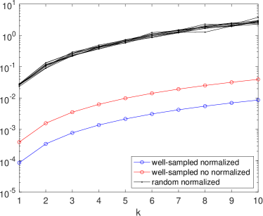
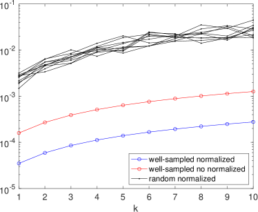
(c)	(d)

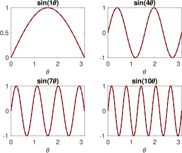
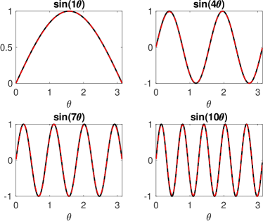
Figure 1: Semi-Circle Example with $n=10000$: (a) Absolute errors of eigenvalues as functions of mode $k$; (b) Root-mean-square errors of eigenvectors as functions of mode $k$; (c) Estimated eigenvectors from well-sampled data, normalized with $m_{o}^{\partial}$; (c) Estimated eigenvectors from random data, normalized with $m_{o}^{\partial}$. In panels (a) and (b), we show estimates from 10 random realizations (black curves).

Based on this result, in the remainder of this paper, all simulations use the normalization $m_{o}^{\partial}$. Figure 1c demonstrates the accuracy of TGL in approximating eigenfunctions for uniformly distibuted data which is well-sampled, while Figure 1d shows the same estimates with random data. We see that even for random data, the approximate eigenfunctions are indistinguishable from the analytic eigenfunctions.

Figure 2 demonstrates convergence as a function of $n$ for both well-sampled uniform data (2a) and random uniformly distributed data (2b). To be consistent with the error metrics in Theorems 4.2 and 4.4, we numerically compute,

$$\begin{aligned} \textup{Error of Eigenvalues}&:=\frac{1}{M}\sum_{i=1}^{M}\frac{|\lambda_{i}-\tilde{\lambda}^{r,\epsilon,n}_{i}|}{|\lambda_{i}|},\\ \textup{Error of Eigenvectors}&:=\frac{1}{M}\sum_{i=1}^{M}\|R_{n}f_{i}-f_{i}^{r,\epsilon,n}\|^{2}_{L^{2}(\mu_{n})},\end{aligned}$$ (35)

where $\{\lambda_{i},f_{i}\}_{i=1}^{M}$ and $\{\lambda_{i}^{r,\epsilon,n},f_{i}^{r,\epsilon,n}\}_{i=1}^{M}$ denote the leading $M$ eigensolutions of the Laplace-Beltrami operator $\Delta$ and the matrix $L^{r}_{\epsilon,n}$, respectively. For non-uniform data, we compute the errors for the leading $M$ eigensolutions $\{\lambda_{i}^{q,r,\epsilon,n},f_{i}^{q,r,\epsilon,n}\}_{i=1}^{M}$ of the matrix $L^{r}_{q,\epsilon,n}$.

In this numerical experiment, we will verify errors correspond to the leading $M=10$ estimated eigensolutions. For random uniformly distributed data, $10$ trials were performed for each value of $n$. In both cases, we still observe convergence faster than the predicted rate of $\mathcal{O}\left(n^{-\frac{1}{8}}\right)$ in this one-dimensional example . Figure 3 shows the errors in Equation (35) for non-uniformly distributed data. The non-uniformly sampled data used to generate Figure 3a (resp. 3b) was distributed in accordance to $\pi\cos(x)$, where $x$ are well-sampled (resp. randomly sampled) data uniformly in the interval $(0,\pi/2)$. With this distribution, there are comparably more data points sampled near the boundary. Again, for random data, $10$ trials were performed for each value of $n$. As expected, the estimations from well-sampled data is more accurate compared to those from randomly sampled data. Nevertheless, in either case we observe convergence as $n\to\infty$ at a rate faster than the rate predicted by the proofs of the main theorems for non-uniformly sampled data.

(a)	(b)

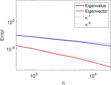
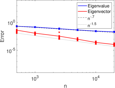
Figure 2: Semi-Circle Example for estimation with $m_{o}^{\partial}$ normalization, uniform sampling distribution. Mean of relative error (eigenvalues) and mean of mean-square-error (eigenvectors) as defined in Equation (35) over the first $M=10$ modes as functions of $n$: (a) Well-sampled data; (b) Random data.

(a)	(b)

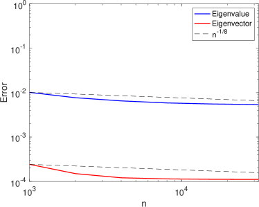
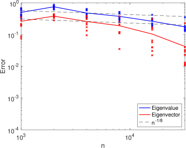
Figure 3: Semi-Circle Example for estimation with $m_{o}^{\partial}$ normalization, nonuniform sampling distribution. Mean of relative error (eigenvalues) and mean of mean-square-error (eigenvectors) as defined in Equation (35) over the first $M=10$ modes as functions of $n$: (a) Well-sampled data; (b) Random data.

6.2 Dirichlet Laplacian on a Semi-Torus

In this example, let $\mathcal{M}$ denote the two-dimensional semi-torus embedded in $\mathbb{R}^{3}$, with standard embedding $\left\{\left((2+\cos\theta)\cos\phi,(2+\cos\theta)\sin\phi,\sin\theta\right):0\leq\phi\leq\pi,0\leq\theta\leq 2\pi\right\}$. We consider the eigenvalue problem

$$\Delta f_{k}=\lambda_{k}f_{k},\qquad f_{k}|_{\partial\mathcal{M}}=0,$$

where $\Delta$ is the Laplace-Beltrami operator on $\mathcal{M}$. It is well known that the Riemannian metric on $\mathcal{M}$ in coordinates $(\theta,\phi)$ is given by

$$g_{\theta,\phi}(u,v)=u^{T}\begin{bmatrix}1&0\\ 0&\sin^{2}\theta\end{bmatrix}v.$$

It can then be checked that the Laplace-Beltrami operator on coordinates $(\theta,\phi)$ takes the form

$$\Delta f_{k}=-\frac{1}{(2+\cos\theta)^{2}}\frac{\partial^{2}f_{k}}{\partial\phi^{2}}-\frac{\partial^{2}f_{k}}{\partial\theta^{2}}+\frac{\sin\theta}{2+\cos\theta}\frac{\partial f_{k}}{\partial\theta}.$$

The eigenvalue problem can then be semi-analytically solved using a separation of variables method. Assuming the solution $f_{k}$ is of the form $f_{k}=\Theta_{k}(\theta)\Phi_{k}(\phi)$, we substitute back into the above and obtain two equations:

$$\Phi^{\prime\prime}_{k}=m_{k}^{2}\Phi,\qquad\Theta^{\prime\prime}_{k}-\frac{\sin\theta}{2+\cos\theta}\Theta^{\prime}_{k}-\frac{m^{2}_{k}}{(2+\cos\theta)^{2}}\Theta_{k}=\lambda_{k}\Theta_{k}.$$

Here, the value of $m_{k}$ will be specified such that $\{\Phi_{k}\}$ satisfy the boundary condition $\Phi_{k}(0)=0=\Phi_{k}(\pi)$. Particularly, $m_{k}=k$ and $\Phi_{k}(\phi)=\sin{k\phi}$. The eigenvalue problem corresponding to the second equation above, subjected to the periodic boundary condition, will be solved numerically with a finite-difference scheme on equal-spaced grid points. We treat eigenvalues and eigenvectors obtained in this semi-analytic fashion as the true solution. This is the same example used in [20] to verify other means (with the Ghost Points Diffusion Maps) for solving the Dirichlet eigenvalue problem.

Well-sampled data was obtained by generating $\sqrt{n}$ data points $\theta_{i}$ uniformly spaced in $[0,2\pi]$, and $\sqrt{n}$ data points $\phi_{i}$ uniformly spaced in $[0,\pi]$. A grid was then constructed, resulting in a total of $n$ data points. For random data, a similar process was employed, but with the data randomly distributed in the corresponding intervals according to a uniform distribution. The spectrum was then approximated using the TGL, normalized with $m_{0}^{\partial}$, as in the previous example. Since the semi-analytical solutions to the above eigenvalue problem used for comparison are represented by vectors, whose components correspond to eigenfunction values at equally spaced grid points (uniformly spaced $64\times 64$ points on intrinsic coordinates),

(a)	(b)

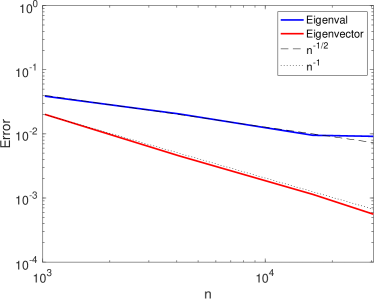
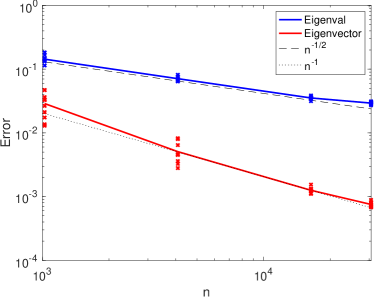
Figure 4: Semi-Torus Example for estimation with $m^{\partial}_{0}$ normalization, uniform sampling distribution. Mean of relative error (eigenvalues) and mean of mean-square-error (eigenvectors) as defined in Equation (35) as functions of $n$: (a) Over the first $M=10$ modes, well-sampled data; (b) Over the first $M=3$ modes, random data.

further considerations were needed to quantify the accuracy of eigenvectors of TGL since they are not necessarily discretized on the same grid points. Particularly, for random (and any well-sampled of different sizes of) data, the Nyström extension method was used to interpolate the TGL eigenvectors to the grid on which the semi-analytic solutions were constructed. Eigenvector error was then evaluated by an average of the mean-square error in Equation (35) on this grid. In both cases, $\epsilon$ was carefully hand-tuned. For well-sampled data, we set $\epsilon=\textrm{.0103,.003, .0008,.0005 }$ for $n=32^{2},64^{2},128^{2},175^{2}$, respectively. For random data, we set $\epsilon=\textrm{.024,.009, .0035,.002}$ for $n=32^{2},64^{2},128^{2},175^{2}$, respectively. Note that for random data, $10$ trials were performed for each value of $n$.

In Figure 4, for both cases of well-sampled and random data, the errors in the estimation of eigenvalues and eigenvectors converges at a rate of $\mathcal{O}\left(n^{-1/2}\right)$ and $\mathcal{O}\left(n^{-1}\right)$, respectively, which are faster than the theoretical estimates. Here, we should point out that the errors for well-sampled data shown in Figure 4(a) are averaged over the leading $M=10$ modes, whereas the errors for random data shown in Figure 4(b) are averaged over the leading $M=3$ modes. We only considered the first $3$ modes in generating Figure 4b since, due to overlapping error in eigenvalues for higher modes for random data, it is unclear which analytic eigenvalue the approximating eigenvalues correspond to without a direct visual comparison of eigenvectors. In this case, the errors in the spectral estimation for higher modes are larger than the differences between consecutive eigenvalues, violating the assumption in Theorem 4.4.

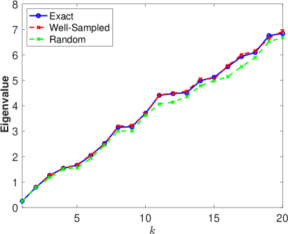
Figure 5: Semi-Torus Example with $n=128^{2}$: Comparison of eigenvalues.

(a)	(b)	(c)

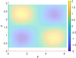
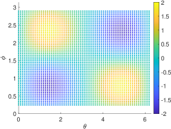
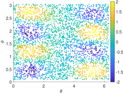
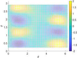
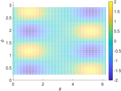
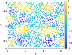
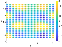
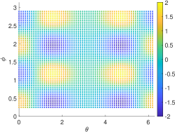
Figure 6: Semi-Torus Example with $n=64^{2}$: Comparison of Eigenvectors in mode 6 (row 1), mode 13 (row 2) and mode 20 (row 3): (a) TGL with Random Data; (b) Nystrom Extension applied to (a); (c) Analytic.

For sufficiently large $n$, the spectral errors are no longer overlapping, and a larger portion of the spectrum can be analyzed, even for random data. In Figure 5, we display the performance of TGL in approximating the spectrum for fixed $n=128^{2}$. For well-sampled data, the approximation and analytic are indistinguishable. For random data, TGL produces an accurate estimate for $k\leq 10$. In Figure 6, we show the eigenvectors of higher modes for $n=64^{2}$. Here, the first column corresponds to the TGL eigenvectors constructed based on randomly distributed data, the second column shows the Nystrom interpolation to the grid points of the semi-analytic solutions, depicted in the third column. This result suggests that although the eigenvalue approximations become less accurate for large modes $k$, eigenvectors of higher modes can be well approximated, even with a relatively small amount of random data. In our numerics (results are not shown), we have seen that the first 20 modes can be well recovered (although they don’t always occur in the same order as the semi-analytic solution when the data is random).

7 Summary

In this paper, we demonstrated a simple proof of the spectral convergence (eigenvalues and eigenvectors) of a symmetrized graph Laplacian to the Laplace-Beltrami operator on closed manifolds by leveraging the result from [25] with the variational characterization of eigenvalues of the Laplace-Beltrami operator. For closed manifolds, the rates obtained are competitive with the best results in the literature. Moreover, using the weak convergence result from [35, 36], we were able to adapt this proof with only slight modifications to demonstrate spectral convergence to the Laplace-Beltrami operator on compact manifolds with boundary satisfying either Neumann or Dirichlet boundary conditions. These results are, to our knowledge, the first spectral convergence results (with rates) in the setting of a compact manifold with Dirichlet boundary condition. The proofs of these results gave simple interpretations of two previously unexplained numerical results. Firstly, the spectral convergence of the Diffusion Maps algorithm on a compact manifold with boundaries to the Neumann Laplacian was fully explained as a combination of the weak consistency, as noted in [36], and the well-known min-max result for the eigenvalues of the Neumann Laplacian on manifolds with boundary. Secondly, the numerical success of the Truncated Graph Laplacian (TGL) in approximating the Dirichlet Laplacian by truncating components of the graph Laplacian matrix corresponding to data points are sufficiently close to the boundary was similarly seen as a combination of the two analogous facts for the Dirichlet Laplacian. Convergence of eigenvectors was obtained by using a method which is adapted from [11]. This method showed the convergence of eigenvectors can be deduced from the convergence of eigenvalues, along with a $L^{2}(\mu_{n})$ norm convergence result. In addition to these proofs, we numerically verified the effectiveness of TGL in approximating the Dirichlet Laplacian for some simple test examples of manifolds with boundary. In these simple examples, we saw that the empirical rate of convergence as $n\to\infty$ is somewhat faster than the theoretical bounds derived this paper when we truncate components of the graph Laplacian matrix corresponding to training data points whose distance from the boundary are less than $\sqrt{\epsilon}$, confirming the discussion in Remark 11.

The spectral convergence results on manifolds with boundary outlined in this paper open up many avenues for future work. First, we suspect that the arguments in this paper can be modified to yield spectral convergence with rates when the discretization $\widetilde{L}_{\epsilon,n}$ is explicitly constructed using $K$-nearest neighbors. To our knowledge, the only other result of this form is reported in [11]. Obtaining a result of this form in the setting of a compact manifold with boundary is of interest, particularly for determining the exact scaling of $K$ to optimize the convergence rate. Second, though rates of convergence of eigenvectors in $L^{2}(\mu_{n})$ norm have been thoroughly investigated, this question remains primarily open for various other norms. Only recently have results for convergence of eigenvectors in $L^{\infty}$ sense been established in [14]. Even so, such results only hold for closed manifolds, and not necessarily compact manifolds with boundaries. Third, though TGL yields convergence to the Dirichlet Laplacian, it is only a slightly modified version of the Diffusion Maps algorithm. It is plausible that further modifications, such as using the ghost points in constructing the TGL matrix as in [16] or other methods such as Ghost Points Diffusion Maps (GPDM) [20], can be shown to converge faster than TGL. Though [20] numerically demonstrated spectral convergence of both modified Diffusion maps and GPDM numerically for various Elliptic PDE’s, the spectral convergence analysis is still an open problem as it involves solving the eigenvalue problem of non-symmetric matrices.

References

- [1] Mikhail Belkin and Partha Niyogi. Semi-supervised learning on manifolds. Machine Learning Journal, 1, 2002.
- [2] Mikhail Belkin and Partha Niyogi. Laplacian eigenmaps for dimensionality reduction and data representation. Neural computation, 15(6):1373–1396, 2003.
- [3] Mikhail Belkin and Partha Niyogi. Towards a theoretical foundation for laplacian-based manifold methods. In International Conference on Computational Learning Theory, pages 486–500. Springer, 2005.
- [4] Mikhail Belkin and Partha Niyogi. Convergence of laplacian eigenmaps. Advances in Neural Information Processing Systems, 19:129, 2007.
- [5] Tyrus Berry and John Harlim. Variable bandwidth diffusion kernels. Applied and Computational Harmonic Analysis, 40(1):68–96, 2016.
- [6] Tyrus Berry and Timothy Sauer. Local kernels and the geometric structure of data. Applied and Computational Harmonic Analysis, 40(3):439–469, 2016.
- [7] Tyrus Berry and Timothy Sauer. Density estimation on manifolds with boundary. Computational Statistics & Data Analysis, 107:1–17, 2017.
- [8] S. Burago and Y. Kurylev. A graph discretization of the laplace beltrami operator. Journal of Spectral Theory, 4:675–714, 2014.
- [9] Jeff Calder and Dejan Slepčev. Properly-weighted graph laplacian for semi-supervised learning. Applied mathematics & optimization, 82(3):1111–1159, 2020.
- [10] Jeff Calder, Nicholas Trillos, and Marta Lewicka. Lipschitz regularity of graph Laplacians on random data clouds. SIAM Journal on Mathematical Analysis, 54(1):1169–1222, 2022.
- [11] Jeff Calder and Nicolas Garcia Trillos. Improved spectral convergence rates for graph laplacians on epsilon-graphs and k-nn graphs. arXiv preprint arXiv:1910.13476, 2019.
- [12] Fan RK Chung and Fan Chung Graham. Spectral graph theory. Number 92. American Mathematical Soc., 1997.
- [13] R.R. Coifman and S. Lafon. Diffusion maps. Applied and Computational Harmonic Analysis, 21(1):5–30, 2006.
- [14] D.B. Dunson, Hau-Tieng Wu, and N. Wu. Spectral convergence of graph laplacian and heat kernel reconstruction in from random samples. Applied and Computational Harmonic Analysis, 55:282–336, 2021.
- [15] John Harlim. Data-driven computational methods: parameter and operator estimations. Cambridge University Press, 2018.
- [16] John Harlim, Shixiao Jiang, Hwanwoo Kim, and Daniel Sanz-Alonso. Graph-based prior and forward models for inverse problems on manifolds with boundaries. arXiv preprint arXiv:2106.06787, 2021.
- [17] John Harlim, Daniel Sanz-Alonso, and Ruiyi Yang. Kernel methods for bayesian elliptic inverse problems on manifolds. SIAM/ASA Journal on Uncertainty Quantification, 8(4):1414–1445, 2020.
- [18] Matthias Hein. Uniform convergence of adaptive graph-based regularization. In International Conference on Computational Learning Theory, pages 50–64. Springer, 2006.
- [19] Matthias Hein, Jean-Yves Audibert, and Ulrike Von Luxburg. From graphs to manifolds–weak and strong pointwise consistency of graph laplacians. In International Conference on Computational Learning Theory, pages 470–485. Springer, 2005.
- [20] Shixiao W Jiang and John Harlim. Ghost Point Diffusion Maps for solving elliptic PDEs on Manifolds with Classical Boundary Conditions. arXiv preprint arXiv:2006.04002, 2020.
- [21] John M Lee. Introduction to Smooth Manifolds. Springer, 2003.
- [22] Jinpeng Lu. Graph approximations to the Laplacian spectra. Journal of Topology and Analysis, pages 1–35, 2020.
- [23] Andrew Y Ng, Michael I Jordan, and Yair Weiss. On spectral clustering: Analysis and an algorithm. In Advances in neural information processing systems, pages 849–856, 2002.
- [24] Mathew Penrose. Random geometric graphs, volume 5. OUP Oxford, 2003.
- [25] Lorenzo Rosasco, Mikhail Belkin, and Ernesto De Vito. On learning with integral operators. Journal of Machine Learning Research, 11(2), 2010.
- [26] Steven Rosenberg. The Laplacian on a Riemannian manifold: An introduction to analysis on manifolds. Number 31. Cambridge University Press, 1997.
- [27] A. Singer. From graph to manifold Laplacian: the convergence rate. Applied and Computational Harmonic Analysis, 21(1):128–134, 2006.
- [28] Amit Singer and Hau-Tieng Wu. Spectral convergence of the connection Laplacian from random samples. Information and Inference: A Journal of the IMA, 6(1):58–123, 2017.
- [29] Ingo Steinwart and Andreas Christmann. Support vector machines. Springer Science & Business Media, 2008.
- [30] Wenqi Tao and Zuoqiang Shi. Convergence of laplacian spectra from random samples. Journal of Computational Mathematics, 38(6):952–984, 2020.
- [31] Erik H Thiede, Dimitrios Giannakis, Aaron R Dinner, and Jonathan Weare. Galerkin approximation of dynamical quantities using trajectory data. The Journal of chemical physics, 150(24):244111, 2019.
- [32] Daniel Ting, Ling Huang, and Michael I. Jordan. An analysis of the convergence of graph laplacians. In Proceedings of the 27th International Conference on International Conference on Machine Learning, ICML’10, page 1079?1086, 2010.
- [33] Nicolás García Trillos, Moritz Gerlach, Matthias Hein, and Dejan Slepčev. Error estimates for spectral convergence of the graph Laplacian on random geometric graphs toward the Laplace–Beltrami operator. Foundations of Computational Mathematics, 20(4):827–887, 2020.
- [34] Nicolas Garcia Trillos and Dejan Slepčev. A variational approach to the consistency of spectral clustering. Applied and Computational Harmonic Analysis, 45(2):239–281, 2018.
- [35] Ryan Vaughn. Diffusion Maps for Manifolds with Boundary. PhD thesis, George Mason University, 2020.
- [36] Ryan Vaughn, Tyrus Berry, and Harbir Antil. Diffusion maps for embedded manifolds with boundary with applications to PDEs. arXiv preprint arXiv:1912.01391v2, 2019.
- [37] Ulrike Von Luxburg, Mikhail Belkin, and Olivier Bousquet. Consistency of spectral clustering. The Annals of Statistics, pages 555–586, 2008.
- [38] Caroline L. Wormell and Sebastian Reich. Spectral convergence of diffusion maps: Improved error bounds and an alternative normalization. SIAM Journal on Numerical Analysis, 59(3):1687–1734, 2021.