Mapping Obscuration to Reionization with ALMA (MORA):
2 mm Efficiently Selects the Highest-Redshift Obscured Galaxies

Abstract

We present the characteristics of 2 mm-selected sources from the largest Atacama Large Millimeter and submillimeter Array (ALMA) blank-field contiguous survey conducted to-date, the Mapping Obscuration to Reionization with ALMA (MORA) survey covering 184 arcmin² at 2 mm. Twelve of thirteen detections above 5$\sigma$ are attributed to emission from galaxies, eleven of which are dominated by cold dust emission. These sources have a median redshift of $\langle z_{\rm 2mm}\rangle=3.6^{+0.4}_{-0.3}$ primarily based on optical/near-infrared (OIR) photometric redshifts with some spectroscopic redshifts, with 77$\pm$11% of sources at $z>3$ and 38$\pm$12% of sources at $z>4$. This implies that 2 mm selection is an efficient method for identifying the highest redshift dusty star-forming galaxies (DSFGs). Lower redshift DSFGs ($z<3$) are far more numerous than those at $z>3$ yet likely to drop out at 2 mm. MORA shows that DSFGs with star-formation rates in excess of 300  M_⊙ yr^-1 and relative rarity of $\sim 10^{-5}$ Mpc^-3 contribute $\sim$30% to the integrated star-formation rate density between $3<z<6$. The volume density of 2 mm-selected DSFGs is consistent with predictions from some cosmological simulations and is similar to the volume density of their hypothesized descendants: massive, quiescent galaxies at $z>2$. Analysis of MORA sources’ spectral energy distributions hint at steeper empirically-measured dust emissivity indices than typical literature studies, with $\langle\beta\rangle=2.2^{+0.5}_{-0.4}$. The MORA survey represents an important step in taking census of obscured star-formation in the Universe’s first few billion years, but larger area 2 mm surveys are needed to more fully characterize this rare population and push to the detection of the Universe’s first dusty galaxies.

1 Introduction

Half of all extragalactic radiation is absorbed by dust and re-emitted at long wavelengths (e.g. Fixsen et al., 1998). Decades of progress, both technological and observational, have taught us that the obscured emission emanates from very different galaxies than unobscured light; the former is largely from massive, star-forming galaxies while the latter is from lower mass galaxies (Whitaker et al., 2017). So while the need to take census of star-formation has been a key focus of extragalactic astrophysics for some time (e.g. Madau & Dickinson, 2014), it has been clear that the very deep surveys of cosmic star-formation conducted in the rest-frame ultraviolet and optical may not adequately capture the full picture. Surveys of submillimeter-luminous dusty star-forming galaxies (DSFGs; e.g. Smail et al., 1997; Blain et al., 2002; Casey et al., 2014) – star-forming galaxies with SFR$\lower 2.15277pt\hbox{$\;\buildrel>\over{\sim}\;$}100\,$ M_⊙ yr^-1 whose stellar emission is over $\;\buildrel>\over{\sim}\;$95% obscured by dust – have been the primary method of unveiling the Universe’s obscured contribution to the star-formation rate density (SFRD). This approach is in direct contrast with the strategy of measuring the total SFRD by taking a census of UV-selected galaxies and correcting estimates for dust attenuation (e.g. as in Bouwens et al., 2020).

A key limitation in all surveys of distant, dust-obscured galaxies is the difficulty in identifying their redshifts. Unlike Lyman Break Galaxies (LBGs), whose selection method directly indicates their redshifts, DSFGs’ spectral shape in the (sub)mm regime is highly degenerate with redshift solutions spanning $1\lower 2.15277pt\hbox{$\;\buildrel<\over{\sim}\;$}z\lower 2.15277pt\hbox{$\;\buildrel<\over{\sim}\;$}12$. Similar efforts to characterize obscured emission indirectly via synchrotron radio emission are faced with similar challenges, though primarily limited to $1\lower 2.15277pt\hbox{$\;\buildrel<\over{\sim}\;$}z\lower 2.15277pt\hbox{$\;\buildrel<\over{\sim}\;$}4$ (Novak et al., 2017). Following up obscured sources in the optical or near-infrared for characteristic emission lines present in star-forming galaxies is difficult due to significant obscuration (Chapman et al., 2003, 2005; Swinbank et al., 2004). Pursuing millimeter spectroscopy has been prohibitive for large samples until recently due to technological and sensitivity limitations in available instrumentation. In addition, the large beamsizes of many single-dish (sub)mm facilities can further obfuscate redshift identification via uncertain astrometry and source confusion, requiring another intermediate stage of interferometric follow-up to constrain positions (e.g. Karim et al., 2013; Hodge et al., 2013).

The complexities in identifying DSFGs’ redshifts has led to great difficulty in measuring the volume density of highly obscured galaxies beyond $z\lower 2.15277pt\hbox{$\;\buildrel>\over{\sim}\;$}3-4$. A small error in redshift measurement for a small fraction of a uniformly-selected DSFG sample (typically selected at $\lambda\leq 1\,$mm) can result in very different inferred volume densities for the population at these redshifts (e.g. see the wide variety of high-$z$ volume density measurements in Rowan-Robinson et al., 2016; Koprowski et al., 2017; Gruppioni et al., 2020; Dudzevičiūtė et al., 2020; Loiacono et al., 2021; Khusanova et al., 2021). This is primarily because the peak in the redshift distribution for 850$\mu$m-selected DSFGs (as well as 1 mm-selected DSFGs) is between $2<z<3$, and sources at higher redshifts are quite rare per unit solid angle on the sky in comparison. This has been demonstrated throughout the literature via the measurement of the redshift distribution of DSFGs selected at $\sim$850$\mu$m–1.2 mm (e.g. Smolčić et al., 2012; Brisbin et al., 2017; Hatsukade et al., 2013). Recent work by Dudzevičiūtė et al. (2020) points out that only 6% of 850$\mu$m-selected galaxies sit at $z>4$. Thus, the accurate identification of such systems – often having degenerate submillimeter colors with sources at lower redshifts – is effectively equivalent to searching for a needle in a haystack.

Some efforts have focused on selecting the highest redshift DSFGs using submillimeter colors, identifying characteristically ‘red’ SEDs across Herschel bands (e.g. Dowell et al., 2014; Ivison et al., 2016; Donevski et al., 2018; Duivenvoorden et al., 2018; Bakx et al., 2018; Yan et al., 2020). However, Herschel bands do not benefit from the negative $K$-correction because they probe emission near the peak of the dust SED rather than the Rayleigh-Jeans tail (Blain, Smail, Ivison, Kneib, & Frayer, 2002; Casey, Narayanan, & Cooray, 2014), thus Herschel datasets tend to have reduced sensitivity to unlensed DSFGs beyond $z\sim 2-3$. Furthermore, this technique may select against high-redshift DSFGs with atypically warm SEDs, due to the degeneracy between dust temperature (or SED peak wavelength, $\lambda_{\rm peak}$) and redshift. There have also been some attempts to constrain the $z\lower 2.15277pt\hbox{$\;\buildrel>\over{\sim}\;$}3$ DSFG population through measurements of anisotropies in the Cosmic Infrared Background (CIB; Maniyar et al., 2018, 2021) though Herschel is largely insensitive to the high redshift tail.

This paper presents data from a new large ALMA mosaic conducted at 2 mm (band 4), whose aim is to efficiently select DSFGs at $z\lower 2.15277pt\hbox{$\;\buildrel>\over{\sim}\;$}3-4$ and measure their volume density at these epochs with more precision than has been done before. This program is called the Mapping Obscuration to Reionization with ALMA (MORA) Survey, for its focus on this especially early epoch of DSFG formation.

The MORA survey is based on the hypothesis that 2 mm dust continuum is an efficient ‘filter’ for $z\lower 2.15277pt\hbox{$\;\buildrel>\over{\sim}\;$}3-4$ systems. Surveys conducted at 850$\mu$m–1.2 mm benefit from the very negative $K-$correction, meaning that their expected flux density is not redshift dependent for a given fixed IR luminosity (i.e. at fixed L_IR, $S_{850}\approx C$, where $C$ is a constant without redshift dependence). Moreover, surveys at 2 mm have an even more extreme negative $K-$correction, such that 2 mm flux density increases with redshift (i.e. at fixed L_IR, $S_{2\,mm}\propto(1+z)^{\eta}$, where $\eta\approx 0.5-1.0$). As a result of this extreme negative $K-$correction, $z\lower 2.15277pt\hbox{$\;\buildrel>\over{\sim}\;$}3$ galaxies of matched luminosity should appear brighter at 2 mm than those at $z\sim 1-3$. This contrasts with nearly every other waveband in which galaxies are observed, from the X-ray through the radio, where more distant objects are expected to be fainter than objects closer to us. If a blank-field 2 mm survey depth is adjusted appropriately, it should be sensitive to detecting DSFGs at $z\lower 2.15277pt\hbox{$\;\buildrel>\over{\sim}\;$}3$ while the much more common $z\sim 1-3$ DSFGs should be undetected (see detailed modeling work in Casey et al., 2018b, a; Zavala et al., 2018a). This is the premise for the design of the MORA survey.

A parallel work to this paper is presented by Zavala et al. (2021), hereafter referred to as Z21, who conduct a number counts analysis of the MORA Survey 2 mm mosaics and implications for the integrated cosmic star-formation rate density at $z\lower 2.15277pt\hbox{$\;\buildrel>\over{\sim}\;$}3$.

This paper presents the characteristics of the individual sources detected in the MORA Survey and what can be inferred about their redshifts, masses, SEDs, and descendants. Section 2 presents the details of the MORA Survey design and data acquisition. Section 3 then presents the identification of the robust sample of 2 mm-selected galaxies, and describes details of each source from what is known in the literature; this section also presents a discussion of sources with low signal-to-noise detections below the formal 5$\sigma$ detection threshold. Section 4 describes models of the 2 mm universe, including semi-empirical models based in cosmological simulations and empirical models. Section 5 presents the main calculations and results of our manuscript, including analysis of the 2 mm population redshift distribution, SEDs, and other unresolved physical characteristics. Section 6 presents a discussion, including results of the contribution of the MORA sample to the cosmic star-formation rate density, an extrapolation of what the MORA galaxy sample will evolve to become, discussion of the measured emissivity spectral index, and the potential impact of cosmic variance on our measurements. Section 7 then presents our conclusions. Throughout we assume a standard $\Lambda$-CDM cosmology adopting the Planck-measured parameters, with $H_{0}=67.4\,$km s^-1 Mpc^-1 (Planck Collaboration et al., 2020), and where SFRs are mentioned, we assume a Kroupa IMF (Kroupa & Weidner, 2003) and scaling relations drawn from Kennicutt & Evans (2012).

Figure 1: The positions of the MORA mosaics shown in teal relative to the entire COSMOS field. The moon is provided for scale in the lower left. Shown are the HST/ACS F814W imaging (Scoville et al., 2007; Koekemoer et al., 2007), the Chandra-COSMOS deep and medium deep survey areas in red (Civano et al., 2016), the CANDELS-COSMOS area in yellow (Grogin et al., 2011; Koekemoer et al., 2011), the deep 450$\mu$m and 850$\mu$m SCUBA-2 pointings in orange from the STUDIES program (Wang et al., 2017) and S2CLS (Roseboom et al., 2013; Geach et al., 2017), and the MORA mosaics in teal. We also show the proposed MORA area (dotted teal square) and the forthcoming PRIMER and COSMOS-Webb deep NIRCam imaging programs (dotted purple lines). Other multiwavelength data are not shown in this figure for clarity, though many cover the full COSMOS field (e.g. deep 3 GHz radio continuum from Smolčić et al., 2017). Most spectroscopy in the field is concentrated within the central 1 deg² around the Chandra-Deep and COSMOS-Webb footprints.

Table 1: MORA Survey Observed Scheduling Blocks, Weather Conditions and Noise Characteristics

Position	Tuning	RA	PWV	On-Source	RMS	Synth.
	[GHz]		[mm]	Time [min]	[$\mu$Jy/beam]	Beamsize
P03	139	10:00:43.83	5.87	44.00	62.8	1$\farcs$85$\times$1$\farcs$46 79o
P03	147	10:00:42.83	4.92	48.82	62.8	2$\farcs$11$\times$1$\farcs$32 72o
P10	139	10:00:29.19	6.19	43.98	98.3	1$\farcs$77$\times$1$\farcs$39 68o
P11	147	10:00:25.96	5.05	48.75	83.5	1$\farcs$51$\times$1$\farcs$45 30o
P12	147	10:00:23.73	4.91	48.78	88.0	1$\farcs$74$\times$1$\farcs$40 54o
P13	147	10:00:21.50	5.68	49.75	87.7	1$\farcs$56$\times$1$\farcs$36 86o
P14	147	10:00:19.26	5.99	49.77	90.9	1$\farcs$68$\times$1$\farcs$33 67o
P15	147	10:00:17.03	2.25	48.78	68.5	2$\farcs$27$\times$1$\farcs$44 72o
P16	147	10:00:14.80	4.72	48.77	112.1	2$\farcs$05$\times$1$\farcs$30 60o
P17	147	10:00:12.57	3.66	48.77	69.2	1$\farcs$94$\times$1$\farcs$44 68o
P18	139	10:00:10.34	5.98	43.98	60.4	2$\farcs$03$\times$1$\farcs$42 68o
P18	147	10:00:10.34	2.98	48.75	60.4	2$\farcs$44$\times$1$\farcs$65 61o
P20	147	10:00:05.87	5.31	48.83	91.1	1$\farcs$82$\times$1$\farcs$36 77o
P03 Mosaic	$-$	$-$	$-$	92.82	62.8	1$\farcs$91$\times$1$\farcs$41 83o
P10–P20 Mosaic	$-$	$-$	$-$	528.91	varies	1$\farcs$83$\times$1$\farcs$43 88o

Table Notes. The range of declinations of pointing centers in each scheduling block is uniform across all SBs and is +02:11:04.16 to +02:33:55.82. The positions (“PXX”) correspond to distinct RAs of the mosaic. Two positions were observed at both frequencies: P03 and P18, while all other positions were only observed with one of the two tunings. Only P10–P20 are spatially adjacent such that they have been stitched together in one contiguous mosaic, and the P03 data is a separate mosaic of its own. This table states the final continuum RMS achieved in each position of the final mosaic product, yet the synthesized beam is measured for a representative subsample of pointings in each individual dataset. The last two rows state the resulting synthesized beams and total on-source time spent for the two end-product mosaics: the P03 mosaic and the P10–P20 mosaic.

2 Data & Observations

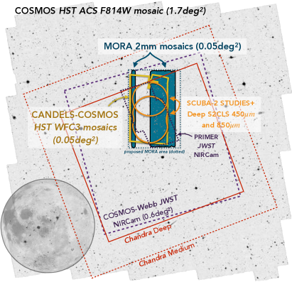
MORA Survey observations were originally designed to cover 230 arcmin² in two tunings, both in ALMA band 4 at 2 mm in the center of the Cosmic Evolution Survey (COSMOS) field (Scoville et al., 2007; Capak et al., 2007; Koekemoer et al., 2007). Figure 1 shows the context of the proposed and observed MORA mosaics in the larger COSMOS field relative to other key datasets in the field. The COSMOS field was chosen as the location of the mosaic due to its rich multiwavelength data (discussed more in § 3.1) and, specifically, the CANDELS portion of the COSMOS field (Grogin et al., 2011; Koekemoer et al., 2011) was chosen for its even deeper near-infrared imaging with Hubble/WFC3. The near-infrared depth will be significantly enhanced with the addition of James Webb Space Telescope (JWST) data from the PRIMER and COSMOS-Webb surveys.

The target continuum RMS for the entire MORA mosaic was 90 $\mu$Jy/beam at 1$\sigma$. This exact tuning configuration in band 4 was chosen based on the program’s secondary goal: to search the known $z\sim 2.5$ protocluster structure, “Hyperion,” which spatially overlaps with this map (Chiang et al., 2015; Diener et al., 2015; Casey et al., 2015; Cucciati et al., 2018), for a blind search of molecular and neutral gas emitters. The first tuning was centered on a local oscillator (LO) frequency of 147.28 GHz (referred to as ‘Tune147’) and covered the frequency ranges 139.5–143.2 GHz and 151.4–155.2 GHz. This tuning is sensitive to the detection of CI(1-0) at $2.44<z<2.52$. The second tuning is centered on a LO frequency of 139.03 GHz and covered the frequency ranges 131.2–134.9 GHz and 143.2–146.9 GHz (referred to as ‘Tune139’). It is tuned to enable the detection of CO(4-3) at $2.42<z<2.51$. This resulted in 21 scheduling blocks of 149 pointings each for each tuning, resulting in 42 total scheduling blocks. Each scheduling block (SB) was spatially distributed as 2 columns of pointings with fixed right ascension and 74–75 pointings in declination spanning a declination range $+$02:11:04 to +02:33:56. Each SB’s fixed R.A. position is referred to as a position and a number in this text, e.g. “PXX” where XX ranges from 03 – 20. As proposed, the mosaic would have covered a total of 3129 pointings at two frequency settings each. The individual pointings of the mosaic were spaced by 19.3″, which is 0.47 times the primary beam FWHM at the highest frequency of data acquisition, 155.2 GHz. This spacing leads to a slightly more compact mosaic than the default Nyquist spacing for mosaics; the same spacing was used for both tunings to make data processing more straightforward. This consequently resulted in a greater depth of observations than proposed (as Nyquist sampling was used to derive the on-source time).

Observations with the Atacama Large Millimeter and submillimeter Array (ALMA) were carried out under program 2018.1.00231.S from 27-March-2019 through 3-April-2019 in the C43-3 configuration for a total of 14.6 hours including overheads and calibrations. Data were acquired under an average precipitable water vapor of PWV = 5 mm with conditions ranging from 2 mm $<$ PWV $<$ 6.5 mm.

The program was observed in part only: 14 of the 42 SBs were executed, 11 of which were at the higher frequency tuning, Tune147, and 3 of which at the lower frequency tuning, Tune139. One of the higher frequency SBs, Tune147 for position P16, did not pass QA0 due to poor weather conditions, but was processed after the fact manually as “semi-pass” data and folded into the final mosaic after flagging problematic antennae. Table LABEL:tab:observations lists the observational conditions and data characteristics of each observed SB and the final mosaics.

There are two final mosaics produced from these data that are spatially distinct: one elongated mosaic represents observations taken in the ‘P03’ position (two pointings wide) with both tunings over a total area of 28 arcmin². P03 is too far spatially offset from the rest of the data to be joined in one mosaic. The other mosaic represents all other data from the spatially adjacent positions ‘P10–P20’ over a total area of 156 arcmin² We refer to these as the ‘P03’ and the ‘P10–P20’ mosaics, respectively. The reason there are two mosaics rather than one is because the program was only partially completed and not all data were taken.

We imaged these data using natural weighting (Briggs weighting with robust=2) to optimize source signal-to-noise. The synthesized beam across all observations was broadly consistent with the beamsize of the final mosaics: 1$\farcs$91$\times$1$\farcs$41 for P03 and 1$\farcs$83$\times$1$\farcs$43 for P10–P20. This beamsize is larger than the characteristic scale of dust in high redshift galaxies ($\sim$0$\farcs$6, e.g. Hodge et al., 2016) but smaller than the minimum anticipated scale of source confusion at 2 mm ($>$20^′′; Staguhn et al., 2014). The synthesized beam is ideally matched to our science goals allowing for the detection of unresolved point sources; therefore, no tapering or alternative data weighting was needed.

Several channels covering a 140 MHz wide frequency range centered on an atmospheric absorption feature at 142.2 GHz were flagged for removal in the Tune147 datasets, while no channels were flagged in the Tune139 datasets. We determined that the channel flagging in the Tune147 datasets improved the RMS depth of the map by 3% on average (see also Zavala et al., 2021).

To analyze the computational time required to produce the full mosaic, we tested time binning the data by 5 s, 10 s, and 30 s. Time binning did substantially speed up the process of combining the visibilities with tclean and the resulting mosaic images were consistent with one another. For our final analysis, we use the 10 s time averaged maps.

Our final mosaics cover 184 arcmin² of the proposed 230 arcmin². Most of the area is in the P10–P20 mosaic (156 arcmin²) while the remaining 28 arcmin² is in the P03 mosaic. Of the full area, 101 arcmin² is covered at or below the proposed depth of 90 $\mu$Jy/beam (with the deepest part of the map reaching 60 $\mu$Jy/beam). See Z21 for more complete information on the noise characteristics of the maps.

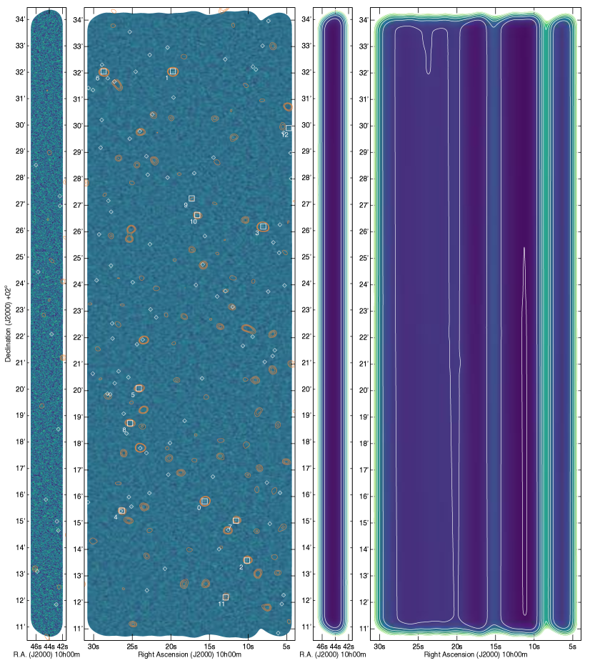
Figure 2 shows both signal-to-noise maps and root-mean-square (RMS) maps of both mosaics. For context, we have overlaid (in contours) the S2COSMOS SCUBA-2 850$\mu$m signal-to-noise map from Simpson et al. (2019).

Figure 2: Signal-to-noise (SNR; left) and root-mean-square (RMS; right) maps of the two MORA mosaics: P03 on the left, and P10-20 on the right. Sources detected at $>$5$\sigma$ significance are enclosed in boxes and numbered, corresponding to the sources listed in Table 3 in decreasing order of SNR. The SCUBA-2 850$\mu$m signal-to-noise map from Simpson et al. (2019) is shown in orange contours, denoting 3.5 $\sigma$, 5 $\sigma$, and 6.5 $\sigma$ significance. Sources detected in the 2 mm map between $4<\sigma<5$ are shown as small diamonds. The RMS maps are overlaid with contours beginning at 60$\mu$Jy/beam and increasing in 30$\mu$Jy/beam steps; the distribution of RMS depths across the full map is shown in Figure 2 of the accompanying MORA Survey paper, Z21. Note that irregularities in the RMS map and discontinuity between the two mosaics are due to the lack of completion of the MORA program.

3 The 2 mm-selected Sample

Extensive tests of large extragalactic mosaics from ALMA (Umehata et al., 2015; Dunlop et al., 2016; Hatsukade et al., 2016; Walter et al., 2016; Aravena et al., 2016; González-López et al., 2019, 2020; Franco et al., 2018, 2020) show that ALMA deep fields exhibit Gaussian noise in the absence of bright (SNR $>$ 10) sources. This is demonstrated for the MORA mosaics in our accompanying paper, Z21, which analyzed the number counts and noise characteristics of this dataset in depth. In Casey et al. (2018a) we simulated completeness and contamination rates for mock ALMA datasets using the assumption that the noise is Gaussian. As argued in § 3.1 of Casey et al. (2018a), the measured contamination rates and completeness of simulated ALMA sources do not depend on the wavelength or underlying number density of sources in the map because they are not confusion-limited.

Z21 tested that confusion is, indeed, not a concern for the MORA mosaics by masking significantly detected sources (of which there are few across the large mosaic) and injecting fake sources through Monte Carlo trials throughout the rest of the map, measuring both completeness and contamination rates as a function of signal-to-noise and 2 mm flux density. Z21 completed the same procedure for fake maps which have Gaussian noise and the same heterogeneous RMS characteristics of our data and find identical rates of contamination and source completeness. Furthermore, we find that sources are recovered at the same rates as simulated in Figure 6 of Casey et al. (2018a), despite the differences in simulated wavelength and different beamsize of observations.

Note that the synthesized beamsize of our observations, $\sim$1$\farcs$9$\times$1$\farcs$4, exceeds the expected full width half maxima of obscured emission for galaxies at $z>1$ ($\sim$1–5 kpc FWHM, corresponding to scales $<$0$\farcs$6, e.g. Simpson et al., 2015; Hodge et al., 2016; Fujimoto et al., 2017), therefore we do not expect any sources to be resolved out beyond the scale of one synthesized beam. Thus the treatment of these sources as point sources rather than sources with extended emission is appropriate and flux densities are measured at the sources’ peak. This contrasts with the recent GOODS-ALMA survey covering 69 arcmin² at 1.1 mm, whose synthesized beamsize of 0$\farcs$6 is similar to the expected size of sources; this led to incompleteness with regard to spatially extended sources in that work and the need to taper observations to recover extended emission (Franco et al., 2018, 2020).

To further diagnose source contamination, we search the MORA maps for significant negative peaks and find 106 sources below $-$4$\sigma$ significance (i.e. strong negative peaks), 15 lower than $-$4.5$\sigma$ and 2 lower than $-$5$\sigma$ significance. With $\sim$3$\times$10⁵ beams in the MORA maps, we expect 48${}^{+6}_{-5}$, 7$\pm$3, and 1$\pm$1 negative sources to arise at these respective significances ($>$ 4, $>$ 4.5 and $>$ 5 $\sigma$). The uncertainties on the expected number of negative noise peaks are determined by generating several fake noise maps with the same noise characteristics as the existing data. The number of negative sources found in the map skews somewhat higher than expected, despite the consistencies of the maps’ noise characteristics with modeled Gaussian noise. Z21 demonstrates that the noise characteristics of the MORA mosaics are indeed Gaussian. We do not suspect that the atypical number of negative sources is from the sidelobes of nearby bright sources. Instead the excess of noise peaks could be due to slight imperfections in modeling the noise. Z21 highlights that the most significant negative detection in the map is found at $-6\sigma$, which only has a $\;\buildrel<\over{\sim}\;$0.5% chance of being generated in a map of this size due to noise. Whether or not this negative detection is of genuine astronomical origin (i.e. potentially a decrement in the CMB caused by inverse compton scattering) is briefly discussed in Z21, but requires further observational follow-up to refute or confirm.

Our tests are consistent with our previous findings in Casey et al. (2018a): sources identified at $>$5$\sigma$ significance have little-to-no contamination with false noise peaks; only 1$\pm$1 false source is expected across both MORA mosaics above this threshold from Gaussian noise. Contamination rises sharply at $4.5<\sigma<5$ significance, consisting of $\sim$ 40 % false noise peaks, and noise peaks come to dominate the sample detected between $4<\sigma<4.5$ significance. In this paper, we present the robust sample of $>5\sigma$ detected sources and then proceed to analyze the marginal $4<\sigma<5$ sample in conjunction with prior identification at other complementary wavelengths. Thirteen $>$5 $\sigma$ sources are identified, one of which is thought to be false, translating to a $>$5$\sigma$ purity of $12/13\approx 92\%$ (a figure that would be higher if real sources were more common).

3.1 COSMOS Ancillary Data

We make extensive use of the rich ancillary data available in the COSMOS field including the two most recent generations of the optical/near-infrared photometric catalog, COSMOS2015 (Laigle et al., 2016) and COSMOS2020 (Weaver, Kauffmann et. al., submitted). There are over 30 bands of optical/near-infrared (OIR) imaging that make up these photometric databases, from deep broadband coverage (with depths of 26–28 magnitudes for 5$\sigma$ point sources) to intermediate and narrow band imaging campaigns (with depths 25–26 magnitudes).

COSMOS also contains a wealth of multiwavelength data, from the X-ray (Civano et al., 2012, 2016) through the radio (Schinnerer et al., 2007; Smolčić et al., 2017). We include details of detections at these other wavebands where relevant. Particularly important for this work are the other millimeter and submillimeter datasets in the field, including SCUBA-2 at 850$\mu$m (Casey et al., 2013; Geach et al., 2017; Simpson et al., 2019), 450$\mu$m (Casey et al., 2013; Roseboom et al., 2013), Herschel PACS and SPIRE at 100–500 $\mu$m (Lutz et al., 2011; Oliver et al., 2012), AzTEC at 1.1 mm (Scott et al., 2008; Aretxaga et al., 2011), and Spitzer at 24$\mu$m (Le Floc’h et al., 2005). In addition, a variety of ALMA archival datasets have built up in the field – see Liu et al. (2018) for details on the A3COSMOS project – at a range in observed frequencies, with the most common tunings in band 6 (1.2 mm) and band 7 (870$\mu$m). We make use of these data to refine the spectral energy distribution fits for galaxies detected in the MORA maps.

3.2 Photometric Redshift Fitting

Photometric redshifts are fit to this existing photometry using the Lephare package and Bruzual & Charlot (2003) templates for star-forming and quiescent galaxies, as in Ilbert et al. (2013). Where OIR photometric redshifts exist for MORA-detected sources, we provide the most recent estimates from COSMOS2020 when available, or in some instances, we use photometric redshifts from elsewhere in the literature. Several photometric redshift catalogs are presented in the COSMOS2020 compilation; we make use of the Classic SExtractor photometry and Lephare photometric redshifts, as we find they minimize $\chi^{2}$ for the redshift estimates. Note that the redshifts overall are indistinguishable from one another for this sample and would not change our results. See Weaver, Kauffmann et. al., submitted for more detail on the differences between these catalogs.

For each source in our sample, we also employ the MMpz technique for FIR/mm photometric redshift fitting described in Casey (2020) as an independent check on redshift constraints at other wavelengths. The MMpz technique uses the aggregate FIR/mm flux density measurements for a source to derive a probability density distribution in redshift. Rather than basing the redshift fit on a single long-wavelength template, MMpz presumes the galaxy is most likely to lie on the correlation between galaxies’ IR luminosities and their rest-frame peak wavelengths, i.e. in the L_IR-$\lambda_{\rm peak}$ plane (as shown in Lee et al., 2013; Strandet et al., 2016; Casey et al., 2018b), and the algorithm determines the redshift range over which the galaxy’s SED is likely to be most consistent with that empirical relationship.

3.3 The 5$\sigma$ subsample

Thirteen sources are identified in our maps above 5$\sigma$ significance. They are numbered in order of decreasing signal-to-noise ratio at 2 mm and their basic detection characteristics are listed in Table 3. Twelve of the thirteen have been detected at other wavelengths and reported in the literature in various forms; in particular, those twelve sources are also detected with SCUBA-2 at 850$\mu$m (Simpson et al., 2019) and with Spitzer IRAC at 3.6$\mu$m. Two of the sources in the sample (sources 5 and 9) have particularly uncertain redshifts and are undetected in deep near-infrared $H$-band imaging from the CANDELS-COSMOS survey (Koekemoer et al., 2011); these two sources and their properties are described in greater detail in the accompanying paper, Manning et. al.

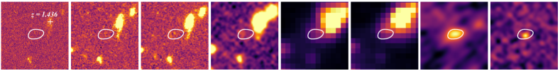
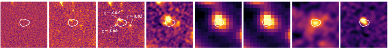
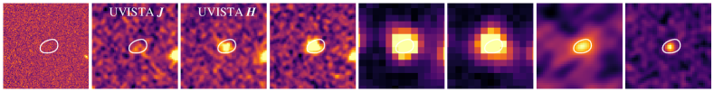
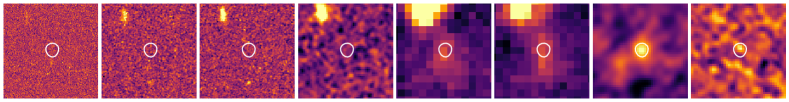
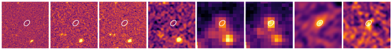
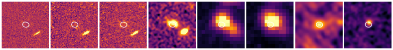
Here we provide a brief summary of each of the $>5\sigma$ sources and the extent to which they have already been characterized in the literature. Table Mapping Obscuration to Reionization with ALMA (MORA): 2 mm Efficiently Selects the Highest-Redshift Obscured Galaxies in the appendix includes additional photometric measurements of each sources’ integrated flux density at all available wavelengths. Figure 3 shows multiwavelength cutouts of all thirteen sources from the optical through the radio.

Figure 3: Multiwavelength cutouts (8${}^{\prime\prime}\times$8^′′, where north is up and east is left) of the 13 sources identified at $>$5$\sigma$ significance at 2 mm (see continuation of this figure on the next page). Cutouts are from HST ACS/F814W (Scoville et al., 2007; Koekemoer et al., 2007), HST WFC3/F125W and WFC3/F160W (Koekemoer et al., 2011; Grogin et al., 2011), Ultra-VISTA $Ks$-band (Laigle et al., 2016), Spitzer 3.6$\mu$m and 4.5$\mu$m (Ashby et al., 2015), 2 mm (this work), and VLA 3 GHz (Smolčić et al., 2017). The sources that sit outside of the CANDELS WFC3 coverage area have $J$ and $H$-band cutouts from Ultra-VISTA shown instead. The 5$\sigma$ contour from the 2 mm imaging is overlaid in each panel for reference. Some sources that sit adjacent to the 2 mm-detected galaxies are labeled with redshifts with more details given in the text.

— Continuation of Figure 3 —

3.3.1 MORA-0, a.k.a. 850.04 or MAMBO-1

The highest signal-to-noise source in the MORA maps is detected at nearly 8$\sigma$, and has been previously identified as a DSFG through detection at 1.2 mm (MAMBO-1 in Bertoldi et al., 2007), 1.1 mm (AzTECC7 in Aretxaga et al., 2011), and at 850$\mu$m (850.04 in Casey et al., 2013). The source is only marginally detected with Herschel SPIRE and SCUBA-2 at 450$\mu$m (Oliver et al., 2012; Casey et al., 2013). To date, it does not have a reliable spectroscopic confirmation despite being targeted repeatedly in near-infared campaigns; the H-band MOSFIRE spectrum presented in Casey et al. (2017) is spatially offset from the ALMA source by 1^′′. The closer (and much fainter) OIR counterpart, only 0$\farcs$3 offset from the ALMA centroid, has an OIR-based photometric redshift from the Laigle et al. (2016) COSMOS2015 catalog of $z_{\rm phot}=3.31^{+0.76}_{-0.81}$; the source is missing from the COSMOS2020 photometric catalogs for no obvious reason other than its marginal detection near the detection limit of the near-infrared catalogs.

MORA-0 has a FIR photometric redshift from Brisbin et al. (2017) of $z_{\rm FIR}=4.4\pm 1.0$. Using the MMpz FIR/mm photometric redshift technique, we derive a mm-based redshift of $z_{\rm mm}=3.4^{+0.6}_{-0.6}$; both FIR/mm photometric redshifts are higher than, though consistent with, the OIR photometric redshift. The source is detected in both the 1.4 GHz and 3.0 GHz radio maps. There are several ALMA programs that have obtained continuum data on MORA-0 in band 6 (1287 $\mu$m and 1250 $\mu$m) and in band 7 (870 $\mu$m). While two radio galaxies were originally thought to be associated with this source (Bertoldi et al., 2007), these are now thought to sit at different redshifts: one with $z_{\rm spec}=1.436$ (reported in Casey et al., 2017) and MORA-0 with a higher photometric redshift. The source at $z=1.436$ is not detected in any of the ALMA data, while MORA-0 is detected in all of bands 4, 6 and 7 where data exists. No millimeter spectroscopy exists for MORA-0.

The lack of detection in the COSMOS2020 photometric redshift catalog, yet detection in COSMOS2015, casts some doubt on the quality of OIR constraints; however, the broad consistency of the COSMOS2015 constraint with the MMpz redshift is reassuring. We adopt the COSMOS2015 photometric redshift throughout the rest of the text.

3.3.2 MORA-1, a.k.a. AzTEC-5

The second most significant source, MORA-1, has been studied under many names, the most widely-used of which is AzTEC-5 for its initial detection in Scott et al. (2008) at 1.1 mm. Magnelli et al. (2019) includes a nice discussion of its known characteristics and redshift constraints, which we summarize here for completeness. AzTEC-5 is Herschel SPIRE, SCUBA-2 (450$\mu$m and 850$\mu$m) and ALMA detected, with continuum measurements in bands 6 and 7.

The literature alludes to a spectroscopic identification for AzTEC-5 of $z=3.791$ based on Ly$\alpha$ emission in a DEIMOS spectrum (Capak et al., 2010; Smolčić et al., 2012); however, that solution was revealed to be inaccurate by subsequent ALMA follow-up that failed to detect emission lines to corroborate the redshift.

Gómez-Guijarro et al. (2018) identify four components of AzTEC-5 in deep near-infrared imaging, which they dubbed AzTEC5-1, 5-2, 5-3, and 5-4. MORA-1 is coincident with the position of AzTEC5-1, which is the only component lacking direct redshift constraints. Gómez-Guijarro et al. do not fit a photometric redshift for AzTEC5-1; it is absent from the COSMOS2020 photometric catalogs. The photometric redshifts for the other components are $z=3.63^{+0.14}_{-0.15}$ for AzTEC5-2, $z=4.02\pm 0.08$) for AzTEC5-3, and $z=3.66^{+0.40}_{-0.43}$ for AzTEC5-4. The redshift constraints on existing components is shown in the third panel (second row) of Figure 3. In addition to AzTEC5-1, AzTEC5-2 also appears to have associated 870-$\mu$m emission, separated from AzTEC5-1 by 0$\farcs$7; ATEC5-2 is not detected at $>$5$\sigma$ significance in our mosaics. Our millimeter-derived photometric redshift for the aggregate photometry of all components of AzTEC-5 give $z_{\rm mm}=2.6^{+2.2}_{-0.8}$, while AzTEC5-1 alone has $z_{\rm mm}=4.8^{+3.7}_{-2.1}$. Due to the significant uncertainties on both, they are consistent with the photometric redshift constraints of the other three components from Gómez-Guijarro et al.

Having detected AzTEC-5 at 2 mm with GISMO, albeit with far worse spatial resolution than the MORA map, Magnelli et al. (2019) argue that the redshift of the entire system is likely $z\sim 3.6$, with substantial obscuration in AzTEC5-1 making it difficult to spectroscopically confirm. Indeed, the close spatial separation $<$1^′′ between the two sources (AzTEC5-1 and AzTEC5-2) would support this claim, as the likelihood of identifying two 870$\mu$m sources with $>$3 mJy at different redshifts separated by $<$1^′′ is exceedingly low (0.02% based on 850$\mu$m number counts; Geach et al., 2017; Simpson et al., 2019). While spectroscopic confirmation is needed for MORA-1, we determine that it is best, for the purposes of this work, to adopt the median redshift of the three other components of the AzTEC-5 system given in Gómez-Guijarro et al. (2018), which is $z_{\rm phot}=3.78^{+0.27}_{-0.32}$.

3.3.3 MORA-2 a.k.a. COS850.0020

The third source in the MORA sample, MORA-2, is detected at a signal-to-noise of 7.6 at 2 mm. It has no match in the earliest SCUBA-2 surveys (Roseboom et al., 2012; Casey et al., 2013) but is detected in the wider-field surveys of COSMOS from Geach et al. (2017) and Simpson et al. (2019). Both ALMA band 6 and 7 data exist for MORA-2, which was selected both as a submillimeter source and dropout source in the ZFOURGE survey (Spitler et al., 2012). Its OIR photometry give a photometric redshift from COSMOS2020 of $z_{\rm phot}=3.36^{+0.60}_{-0.28}$. There are no spectroscopic constraints for MORA-2; our millimeter-derived photometric redshift for the source is $z_{\rm mm}=2.8^{+0.6}_{-0.6}$ which is consistent with the OIR photometric redshift.

3.3.4 MORA-3, a.k.a. AzTEC-2 or 450.03

The fourth source, MORA-3, is more widely known as AzTEC-2 (Younger et al., 2007) detected with the SMA, and at 450$\mu$m and 850$\mu$m by SCUBA-2 (where it is known as 450.03; Casey et al., 2013). It was also previously detected at 2 mm as GISMO-C2 (Magnelli et al., 2019). It is detected by Herschel SPIRE and has ALMA continuum data in band 6 and 7. The interferometric data reveal two millimeter sources, the primary (coincident with the 2 mm emission) is AzTEC2-A and the secondary fainter source (detected at 2.6$\sigma$ significance in the 2 mm map) is AzTEC2-B. While a spectroscopic identification based on a possible OIR counterpart existed at $z=1.123$ (Smolčić et al., 2012; Casey et al., 2017) 1^′′ to the south of the primary source A, that redshift has since been shown to be associated with a foreground galaxy.

The spectroscopic redshift of AzTEC-2 is now confirmed through the detection of [Cii] and CO(5-4) at $z=4.63$ by Jiménez-Andrade et al. (2020); this was independently confirmed in Simpson et al. (2020). AzTEC2-A has a spectroscopic redshift of $z=4.625$ while AzTEC2-B is at $z=4.633$. Our millimeter-derived photometric redshift for this source is consistent with its spectroscopic identification, $z_{\rm mm}=3.3^{+1.0}_{-0.8}$. Both components of AzTEC-2 are undetected in existing HST deep imaging, and the Spitzer imaging is highly confused with two foreground galaxies: the $z=1.123$ galaxy 1^′′ to the south of AzTEC2-A and an elliptical galaxy at $z=0.34$ at 1^′′ south of the $z=1.123$ system. Both components of AzTEC-2 are detected at 3 GHz in radio continuum. See Jiménez-Andrade et al. (2020) for a more thorough discussion of this source.

Given the proximity of the foreground elliptical galaxy at $z=0.34$, Jiménez-Andrade et al. (2020) estimate that the luminosity of AzTEC2-A, or MORA-3, is gravitationally lensed by a magnification factor of $\mu=1.5$. We scale physical quantities proportional to luminosity by this magnification factor for MORA-3 for the rest of this paper. Note that this source sits in a large scale overdensity at $z=4.6$ identified and described in Mitsuhashi et al. (2021), further corroborating the conjecture that high star-formation rate galaxies at $z>4$ are highly clustered and good signposts for the most massive overdense structures in the Universe (Casey, 2016; Chiang et al., 2017).

3.3.5 MORA-4, a.k.a. MAMBO-9

The fifth source of the sample, MORA-4, is known as MAMBO-9. It was originally detected at 1.2 mm by the MAMBO instrument (Bertoldi et al., 2007), and subsequently detected at 1.1 mm (as AzTEC/C148; Aretxaga et al., 2011) and SCUBA-2 at 850$\mu$m (as 850.43 and COS.0059 in Casey et al., 2013; Geach et al., 2017, respectively). Several teams identified the source as potentially high-$z$ based on being undetected in the Herschel SPIRE bands; Jin et al. (2019) initially report a spectroscopic identification of $z=5.850$ based on a low signal-to-noise 3 mm spectral scan, confirmed by detection of ¹²CO($J\!=$6$\rightarrow$5) and p-H₂O(2${}_{1,1}\!\rightarrow$2_0,2) in Casey et al. (2019). MAMBO-9 is comprised of two galaxies separated by 6 kpc (1^′′) and both confirmed at $z=5.850$. Our millimeter-derived photometric redshift for MAMBO-9 is $z_{\rm mm}=5.1^{+0.6}_{-0.8}$, only in slight tension with the measured spectroscopic redshift. MAMBO-9 is the most distant unlensed DSFG found to-date and we refer the reader to Casey et al. (2019) for a more thorough characterization of the MAMBO-9 system.

3.3.6 MORA-5 a.k.a. 850.13 or AzTEC C114

The sixth source, MORA-5, has been identified at both 850$\mu$m and 1.1 mm (Casey et al., 2013; Aretxaga et al., 2011, named 850.13 and AzTEC C114, respectively). There is no spectroscopic redshift for MORA-5, and there is no OIR-based photometric redshift from either the COSMOS2015 or COSMOS2020 catalogs due to a lack of counterpart in the near-infrared. Brisbin et al. (2017) offer a FIR photometric redshift of $z_{\rm FIR}=5.3\pm 3.2$, while noting that a radio-FIR-based photometric redshift is consistently lower, based on the source’s detection at both 1.4 GHz and 3 GHz (respective radio-FIR photometric redshifts of $z_{\rm 1.4GHz}=2.9^{+4.2}_{-0.4}$ and $z_{\rm 3.0GHz}=1.9^{+1.1}_{-0.3}$). Our millimeter-derived photometric redshift is $z_{\rm mm}=3.4^{+1.1}_{-0.9}$. This source is undetected at all wavelengths shortward of 3.6 $\mu$m, including deep CANDELS $H$-band and Ultra-VISTA $K$-band imaging. Our accompanying paper, Manning et. al., present a more detailed analysis of this source and calculate a hybrid photometric redshift estimate for the source of $z_{\rm phot}=4.3^{+1.5}_{-1.3}$ combining the MMpz redshift with direct extraction and refitting of OIR constraints using both eazy and magphys approaches (see Manning et. al. for more details). We adopt the Manning et. al. hybrid photometric redshift for the rest of this paper.

3.3.7 MORA-6 a.k.a. 450.00

The seventh source, MORA-6, was detected as the brightest 450$\mu$m source, named 450.00, in the 394 arcmin² map in Casey et al. (2013). This source is also detected at 850$\mu$m with SCUBA-2 and has ALMA continuum follow-up in both bands 6 and 7. It lacks a spectroscopic redshift but does have a fairly well-constrained OIR-based photometric redshift of $z_{\rm phot}=3.34^{+0.13}_{-0.12}$ from COSMOS2020. Our millimeter-derived photometric redshift is $z_{\rm mm}=2.5^{+1.6}_{-0.7}$, consistent with the OIR photometric redshift.

3.3.8 MORA-7 a.k.a. 850.53

The eighth source, MORA-7, has been previously identified at 850$\mu$m in both Casey et al. (2013) as 850.53 (lacking a corresponding detection at 450$\mu$m) and Geach et al. (2017) as COS850.0035. This source lacks a spectroscopic redshift, but is detected with Spitzer and Ultra-VISTA, rendering an OIR photometric redshift estimate of $z_{\rm phot}=2.85^{+0.24}_{-0.33}$. The source has dust continuum observations from ALMA in both bands 6 and 7. Our millimeter photometric redshift is $z_{\rm mm}=2.3^{+2.7}_{-0.8}$, consistent with the OIR photometric redshift.

3.3.9 MORA-8 a.k.a. 850.09

The ninth source of our sample, MORA-8, has been previously identified at both 450$\mu$m and 850$\mu$m in Casey et al. (2013) wherein it was referred to as 850.09 and in Geach et al. (2017) where it was named COS850.0016. The source lacks spectroscopic confirmation, but the OIR photometric redshift from COSMOS2020 is fairly well-constrained as $z_{\rm phot}=2.29^{+0.12}_{-0.08}$. This source also has ALMA band 7 continuum data, from which our millimeter-derived redshift is $z_{\rm mm}=3.0^{+2.2}_{-1.0}$. Both ALMA 2 mm and 870 $\mu$m sources are well aligned with the OIR counterpart.

3.3.10 MORA-9

The tenth source of the sample, MORA-9, has been detected at 850$\mu$m in Simpson et al. (2019) at 4.4$\sigma$ significance; it had not been detected in the earlier compilation of Geach et al. (2017). Aside from its detection at 2 mm and 850$\mu$m, the source is also detected at 3.6$\mu$m and 4.5$\mu$m from Spitzer and at low significance in Ultra-VISTA $K$-band imaging. This source is undetected in all other datasets, but its $K$-band counterpart renders it present in the COSMOS2020 photometric catalogs with an OIR photometric constraint of $z_{\rm OIR}=4.57^{+1.33}_{-1.22}$. It is one of only two $>$5$\sigma$ sources not already surveyed by ALMA at other wavelengths (the other being MORA-12). The ratio of 850$\mu$m-to-2 mm flux density is highly suggestive of a high-$z$ solution; we derive a millimeter photometric redshift of $z_{\rm mm}=5.5^{+0.6}_{-0.8}$ for this source. Manning et. al. describe this source’s characteristics and derive a hybrid photometric redshift for MORA-9 of $z_{\rm phot}=4.3^{+1.3}_{-1.0}$ which includes this millimeter photometric redshift along with OIR constraints using photometric redshift fitting techniques eazy and magphys. We adopt the Manning et. al. hybrid photometric redshift for the rest of this paper.

3.3.11 MORA-10, a.k.a. 450.09

The eleventh source of our sample, MORA-10, is well characterized as a known DSFG detected at both 450$\mu$m and 850$\mu$m from SCUBA-2 (named 450.09; Casey et al., 2013), with a near-infrared spectroscopic redshift of $z=2.472$ as reported in Casey et al. (2015). The source is one of many DSFGs in the COSMOS field that sits in a protocluster environment at $z\sim 2.5$, the same structure that motivated the dual spectral tunings for the MORA program (Chiang et al., 2015; Diener et al., 2015; Casey et al., 2015; Cucciati et al., 2018). ALMA data exists for 450.09 in both band 7 and band 3, where the band 3 data confirm its spectroscopic redshift via detection of CO(3-2). The millimeter photometric redshift for the source is $z_{\rm mm}=4.5^{+1.4}_{-1.0}$, which is 2$\sigma$ discrepant with the measured spectroscopic redshift (this discrepancy originates from the galaxy appearing to be a bit colder than the average SED).

MORA-10 is unique among the MORA Survey sample for being particularly luminous in its radio continuum ($S_{\rm 1.4\,GHz}=5.7$ mJy and $S_{\rm 3.0\,GHz}=3.2$ mJy) with a rest-frame radio luminosity of $L_{\rm 178\,MHz}=1.9\times 10^{27}$ W Hz^-1, nearly bright enough to fit the local Fanaroff-Riley class II radio-loud AGN (Fanaroff & Riley, 1974) definition at its redshift. Fitting the existing radio continuum measurements to a powerlaw, we derive a synchrotron slope of $\alpha=0.85$; extended to the observed 2 mm band data, we estimate a total synchrotron contribution of $S_{\rm 2mm,synch}=159\pm 60$ $\mu$Jy toward the total observed $S_{\rm 2mm}=405\pm 78\,$$\mu$Jy. This implies that $\approx$ 39$\pm$17% of the total measured 2 mm flux density is due to synchrotron processes. While this clearly does not dominate the total flux density, an absence of synchrotron emission in this source would have rendered it below the 5$\sigma$ detection limit of our sample. Even if the synchrotron sloped varied somewhat, the source would have not been detected at high significance from its dust emission alone once its synchrotron component is subtracted from the total 2 mm flux density. Because the primary goal of this work is to identify thermal dust emission at 2 mm, we will exclude MORA-10 from analysis of population statistics, like its contribution to the 2 mm-selected galaxy redshift distribution and star formation rate density. For MORA-10’s far-infrared/millimeter SED fit, we adjust the 2mm flux density to only account for the estimated dust continuum component, removing the synchrotron component, as we are only fitting the dust SEDs in this paper.

3.3.12 MORA-11 a.k.a. AzTECC76 or COS.0194

The penultimate source of the sample, detected at 5.2$\sigma$ significance, is MORA-11. It is detected at 850$\mu$m in both Geach et al. (2017), where it was named COS.0194, and in Simpson et al. (2019). It is also detected at 1.1 mm from Aretxaga et al. (2011) and in the Herschel SPIRE bands at 250–500$\mu$m. Broadly detected in the near-infrared through radio, MORA-11 has a reported medium-band survey redshift of $z=3.17\pm 0.12$ from the NEWFIRM Medium Band Survey (Whitaker et al., 2011); the source has additional Keck-NIRSPEC $K$-band spectroscopic observations from Marsan et al. (2017), though no emission lines were detected. This redshift is in agreement with its OIR photometric redshift from COSMOS2020 of $z_{\rm phot}=3.00^{+0.10}_{-0.13}$. We measure a millimeter photometric redshift of $z_{\rm mm}=4.3^{+4.9}_{-1.2}$ for this source. We adopt the medium-band photometric redshift for MORA-11 for the rest of our analysis in lieu of the COSMOS2020 photometric redshift due to the improved precision offered by the spectro-photometric analysis of Marsan et al. (2017). Note that spectral analysis of our own MORA mosaic has tentatively identified an emission line at 140.85 GHz, which could be CO(5-4) at $z=3.091$, consistent with the adopted redshift of $z=3.17\pm 0.12$; further analysis of this line identification is in progress (Mitsuhashi et. al., in prep).

3.3.13 MORA-12

The last source in our sample, MORA-12, is detected at 5.02$\sigma$ significance; unlike the rest of the $>$5$\sigma$ sample, it has no corresponding detection at 850$\mu$m. While there is a 850$\mu$m source (with strong 24$\mu$m emission, named 850.77 in Casey et al., 2013) 9.6^′′ away from the ALMA 2 mm position, we think it is unlikely that the two are associated. MORA-12 is also not detected in the Herschel COSMOS maps, as well as the GISMO map from Magnelli et al. (2019). This source is the only source in the $>$5$\sigma$ sample to lack detection in Spitzer IRAC at 3.6$\mu$m or 4.5$\mu$m. There is no additional ALMA data at any other wavelength at the position of MORA-12. With only one detection at one wavelength, we are unable to derive a millimeter photometric redshift for this source. Because it has not been detected at any other wavelength, sits on the boundary of the P10-P20 mosaic, and given our expected contamination rate of 1$\pm$1 false source detected above the 5$\sigma$ threshold, we conclude it most likely that MORA-12 is not real and that it is a positive noise peak.

3.3.14 Summary Characteristics of $>$5$\sigma$ Sample

Of the thirteen sources detected at $>$5$\sigma$, we determine that twelve of them are real 2 mm-detected galaxies while the last and least significant (MORA-12) is likely a positive noise peak. Of the twelve real sources, all are detected with both Spitzer IRAC and SCUBA-2 at 850 $\mu$m. Despite all being previously detected, not all sources had been identified as high-$z$ candidates. One of the twelve sources (MORA-10) is thought to have a substantial contribution (39$\pm$17%) from synchrotron radio emission to its 2 mm flux density, rendering the sample of purely dust-selected 2 mm sources with only eleven galaxies.

Three of the twelve sources are spectroscopically-confirmed at $z=2.472$ (MORA-10, a.k.a. 450.09, with the synchrotron component), $z=4.625$ (MORA-3, a.k.a. AzTEC-2), and $z=5.850$ (MORA-4, a.k.a. MAMBO-9); of the remaining nine sources, eight have some form of OIR-based photometric redshift (Laigle et al., 2016; Marsan et al., 2017; Gómez-Guijarro et al., 2018, Weaver, Kauffmann et. al., submitted). The last source (MORA-5) lacks an OIR counterpart and any redshift constraint; MORA-5 along with MORA-9, whose OIR phot-$z$ is highly uncertain, have hybrid photometric redshift fits provided in our accompanying manuscript, Manning et. al.

Four of the 11 dust-selected sources (36%) are “OIR-dark,” meaning they lack near-infrared $H$-band counterparts in deep WFC3 imaging, which in this case is CANDELS-COSMOS data reaching a 5$\sigma$ point source depth of 27.15 (Koekemoer et al., 2011). These sources are MORA-3 (a.k.a. AzTEC-2, spectroscopically confirmed at $z=4.63$), MORA-4 (a.k.a. MAMBO-9, spectroscopically confirmed at $z=5.85$), MORA-5 and MORA-9. As these represent the potential highest redshift subset of the 2 mm-selected sample, a more thorough analysis of them is given in the accompanying paper by Manning et. al.. It appears that MORA-3 (AzTEC-2) is the only galaxy in the sample that is gravitationally lensed ($\mu=1.5$; Jiménez-Andrade et al., 2020).

The majority of the MORA 2 mm-selected galaxy sample is consistent with relatively little AGN activity, or AGN activity that does not dominate the galaxies’ bolometric luminosities. We investigate the sample’s AGN content by analyzing X-ray imaging, radio emission, and mid-infrared emission. None of the $>5\sigma$ sample is detected in the deep COSMOS Chandra or XMM data, though the sensitivity of such X-ray surveys is rather shallow at $z>3$. The galaxies’ radio luminosities measured at 3 GHz (Smolčić et al., 2017), and in the somewhat shallower 1.4 GHz data, are in line with expectation for synchrotron emission generated via star-formation processes instead of AGN (e.g. Yun et al., 2001; Ivison et al., 2010; Delhaize et al., 2017). The one source that proves an exception to this is MORA-10, which appears to be radio-loud and whose 2 mm emission is partially dominated by such non-thermal emission mechanisms. In the mid-infrared, five of eleven (5/11=45%) are 24$\mu$m-detected. Aside from MORA-10 which clearly has an AGN, three of the other four 24$\mu$m-detected galaxies are the lowest redshift sources in the sample (MORA-6, -7, and -8), which, at those redshifts, could be due to either AGN or star-formation via PAH emission. The last 24$\mu$m detection, MORA-1, is a blend of several sources $z\sim 3.6-4.0$ and the centroid of the emission is not precisely constrained to the 2 mm source in question. While AGN overall seem non-dominant in this sample of 2 mm-selected DSFGs, it should be noted that recent modeling work has shown that AGN can contribute substantially to the heating of host galaxy-scale dust, even in IR-luminous galaxies without prominent AGN (McKinney et al., 2021); such effects are difficult to account for without constraining observations, thus we do not account for it directly in this work.

3.4 Marginal Sources with $<$5$\sigma$ significance

Below the 5$\sigma$ threshold, contamination from positive noise peaks becomes a significant concern. There are 87 sources identified in the MORA P10-20 mosaic and 11 sources found in the P03 mosaic at $4<\sigma<5$ significance, or 98 in total. Their positions and characteristics are given in Table Mapping Obscuration to Reionization with ALMA (MORA): 2 mm Efficiently Selects the Highest-Redshift Obscured Galaxies. We determine which of these sources are most likely to be real by testing for coincident identification at other wavelengths, for example, in the COSMOS2015 catalog, the COSMOS2020 catalog, the 3 GHz radio continuum survey (Smolčić et al., 2017), or at 850$\mu$m from SCUBA-2 (Simpson et al., 2019).

Given the high source density of galaxies in the OIR catalogs, there is a 8% chance of a random point in our map aligning with a COSMOS2015 counterpart within 1^′′ (which is conservative maximum physical scale on which we see spatial offsets of obscured and unobscured emission in galaxies, e.g. Biggs & Ivison, 2008, with more characteristic scales of 0$\farcs$1–0$\farcs$3, as in Cochrane et al. 2019). The probability of a chance alignment with a source in COSMOS2020 is slightly higher within 1^′′, $\sim$13%, given its increased depth at near-infrared wavelengths. Out of a sample of 98 marginal sources, this would suggest a total of 8$\pm$3 sources matched at random to COSMOS2015 and 13$\pm$4 sources matched at random to COSMOS2020. We find a total of 12 matches to COSMOS2015 and 17 matches to COSMOS2020 within the MORA $4<\sigma<5$ 2 mm sample (11/12 overlap between COSMOS2015 and COSMOS2020), suggesting that there are very few real sources ($<1/3$) in this marginal sample and none that can be directly identified reliably.

We also tested the correlation between the marginal sample with 850$\mu$m-selected DSFGs observed by SCUBA-2 (Simpson et al., 2019); we find that there should be a 2.9% chance of random alignment between a $>3.5\sigma$ SCUBA-2 source (within the SCUBA-2 15^′′ FWHM beam) and a marginal source in our 2 mm catalog. The rate of false positives is lower for 850$\mu$m counterparts than for OIR counterparts because the sky density is much lower for 850$\mu$m sources. We find twelve sources that are spatially coincident with a 850$\mu$m SCUBA-2 source (a total of 12% of the marginal sample), well in excess of the anticipated $\sim$3%. Contrary to our findings using OIR counterparts, this demonstrates a true excess of real sources within the marginal sample. Of these twelve sources, three have secure IRAC 3.6$\mu$m counterparts matched to the positions of the 2 mm emission, corroborating their identification as real sources.

We further investigate radio continuum counterparts for the marginal sample using the 3 GHz radio continuum map in COSMOS presented in Smolčić et al. (2017). Some of the sources are also covered by the deeper COSMOS-XS survey (van der Vlugt et al., 2021; Algera et al., 2020). We find that there is a 0.6% chance of random alignment between a marginal MORA source and a 3 GHz $>5\sigma$ detected source within 1^′′ of one another. The rate of false positives is lowest for radio counterparts due to their increased rarity on the sky, in addition to their precisely measured positions. We find that six MORA 2 mm sources are spatially coincident with a 3 GHz radio continuum source (a total of 6% of the marginal sample), a factor of ten higher than the anticipated $\sim$0.6%. The strength of this excess is such that the 3 GHz-detected subset can be reliably identified as having real 2 mm emission. Nevertheless, the sample is somewhat limited in size to analyze in further detail.

We include an abbreviated table of marginally-detected $4<\sigma<5$ 2 mm sources in Table Mapping Obscuration to Reionization with ALMA (MORA): 2 mm Efficiently Selects the Highest-Redshift Obscured Galaxies for reference and note which sources have counterparts at which wavelengths. However, due to high contamination rates and a similarly high incompleteness rate in this flux density regime, we do not analyze the sample further. Later in § 5.5 we analyze the 2 mm emission properties of any DSFGs that have been independently observed by ALMA (not a part of MORA) in the field, some of which overlap with this marginal sample.

The lack of reliability of the marginal sample is further verified by analyzing the number of negative peaks in the mosaics between 4–5$\sigma$, of which there are a total of 106. If there were a significant population of real sources embedded in the marginally-identified sample, the positive peaks (98) would likely outnumber the negative peaks (106).

4 Models of the 2mm Universe

We make use of several cosmological semi-empirical and empirical models of the 2 mm-luminous Universe to draw comparisons with the MORA dataset. A brief description of each model dataset follows.

First, we compare to the Simulated Infrared Dusty Extragalatic Sky (SIDES) model (Bethermin et al., 2017), which builds galaxies’ SEDs from their stellar masses and star formation rates (assuming a bimodal population of main sequence galaxies and starbursts) and which updates the 2SFM (2 Star Formation Modes) galaxy evolution model (Béthermin et al., 2012; Sargent et al., 2012) to analyze the impact of clustering on IR map analysis. The 2SFM model posits that there is a bimodal population of star forming galaxies: those that are on the main sequence and starbursts that have elevated specific star formation rates; the 2SFM model uses this framework to model all galaxies. We make use of the full SIDES 2 deg² lightcone in our analysis, both to sample cosmic variance and understand possible trends for 2 mm-selected galaxies on angular scales larger than the MORA survey.

Second, we compare our results to the Shark semi-analytic model of galaxy formation (Lagos et al., 2018). By using the SED code ProSpect (Robotham et al., 2020) and the radiative transfer analysis of the EAGLE hydrodynamical simulations of Trayford et al. (2020), the Shark model was successfully able to predict the ultraviolet to far-infrared emission of galaxies over a wide range assuming a universal IMF (Lagos et al., 2019). Lagos et al. (2020) presents detailed predictions for the (sub-)millimeter galaxy population, including 2 mm number counts and redshift distributions. We make use of the full 108 deg² Shark lightcone for our comparisons.

Third, we compare our work to the semi-empirical model for dust continuum emission published by Popping et al. (2020); that work primarily focused on comparison of 850$\mu$m and 1.1 mm number counts and redshift distributions with the ASPECS survey results (Aravena et al., 2020; González-López et al., 2019, 2020). Using the same methodology of Popping et al., several lightcones from the UniverseMachine framework (Behroozi et al., 2018), which is grounded in the Bolshoi-Planck dark matter simulation (Klypin et al., 2016; Rodríguez-Puebla et al., 2016), are stitched together to form a 7.7 deg² lightcone. Dark matter halos are populated with galaxies calibrated to observationally constrained relations (in stellar mass and SFR distributions), and dust continuum characteristics are applied using the relations derived in Hayward et al. (2011, 2013) using the SUNRISE (Jonsson, 2006) dust radiative transfer code as a function of SFR and dust mass.

Lastly, we compare to the empirical model predictions for the submillimeter sky presented by Casey et al. (2018b, a) and expanded on in Zavala et al. (2018a) and, finally, in Z21. The key difference between the Casey et al. (2018b) models and the cosmological semi-empirical models is the built-in flexibility to test different hypothetical evolving infrared luminosity functions against data. Not tethering this model directly to any cosmological simulation renders it a tool to interpret data that may be discrepant with such simulations. Casey et al. (2018b) use it to present the hypothetical (sub)mm sky in two diametrically opposed Universes: the ‘dust poor’ Universe (model A) in which there is steep evolution from $z\sim 7$ to $z\sim 2$ in the characteristic number density of the IRLF ($\Phi_{\star}$), and the ‘dust rich’ Universe (model B), in which the evolution of the characteristic number density is much more shallow. The ‘dust poor’ Universe effectively translates to a very minor contribution of intense, dusty starbursts to cosmic star formation beyond $z\lower 2.15277pt\hbox{$\;\buildrel>\over{\sim}\;$}5$ ($<$10%), while they would dominate cosmic star formation at similar epochs in the ‘dust rich’ Universe ($>$90%). These models are built to capture two extremes. Zavala et al. (2018a) uses 3 mm number counts from the ALMA archive to argue for a solution between these two extremes. Our accompanying paper, Zavala et al. (2021) presents an update to Zavala et al. (2018a) using MORA 2 mm number counts, updated 3 mm archival counts, as well as deep 1 mm number counts from the ASPECS survey (Aravena et al., 2020; González-López et al., 2019, 2020). The expanded dataset used to constrain the model in Zavala et al. (2021) relative to Zavala et al. (2018a) has resulted in a change of the predicted $z\lower 2.15277pt\hbox{$\;\buildrel>\over{\sim}\;$}2$ evolution of $\Phi_{\star}$, the number density of DSFGs at early times, from $\Phi_{\star}\propto(1+z)^{-4.2}$ to $\Phi_{\star}\propto(1+z)^{-6.5}$ (see Zavala et al., 2021, for more details).

5 Results

Figure 4: Comparison of the redshift probability density distributions derived from: the FIR/mm using the MMpz technique (teal distributions), OIR photometric redshifts (blue distributions), and spectroscopic constraints (black lines). The hashed regions of those same colors indicate the 68 percentile inner confidence interval. Sources are ordered by redshift, from highest (top) to lowest (bottom). The two unconfirmed OIR-dark sources with the most uncertain redshift constraints are MORA-5 and MORA-9, described in more detail in our accompanying manuscript, Manning et. al.. The redshifts for these two galaxies are derived jointly using OIR and millimeter constraints, here called hybrid.

5.1 Redshift Constraints & Distribution

Redshift constraints for our sample are heterogeneous, ranging from firm spectroscopic confirmations to limited far-infrared/millimeter photometric constraints. We exclude MORA-10 (which has $z_{\rm spec}=2.472$) from analysis of the sample’s redshift distribution due to the suspected contribution of synchrotron emission to its 2 mm flux density, without which it would not have been detected above 5$\sigma$ in our data.

Figure 5: The measured cumulative redshift distribution for the eleven dust-continuum dominated 2 mm galaxies detected in the MORA maps compared to literature models. Each galaxy’s redshift probability density distribution is coadded here to reflect the uncertainty in the total CDF; we measure the uncertainty on the median redshift estimate, $\langle z_{\rm 2mm}\rangle=3.6^{+0.4}_{-0.3}$, through Monte Carlo draws from the CDF. Literature model redshift CDFs are measured by drawing galaxies from the model with matched flux densities to our real sources (within uncertainties) and inferring the redshift distributions of those sources. The left panel compares to three hypothetical universe predictions using the Casey et al. (2018b) model framework: the Casey et. al. “dust poor” model A Universe (blue), the “dust rich” model B Universe (orange), and the Zavala et al. (2018a) 3 mm-number counts based model (green). The right panel compares with three other models: the SIDES model (purple; Bethermin et al., 2017), the SHARK model (red; Lagos et al., 2020), and the most recent 1 mm/2 mm/3 mm updated number counts-based model from Z21. Note that the Z21 model is largely based on our MORA maps, but it does not use any source redshift information as input, and thus its redshift distribution predictions are derived independent of these data.

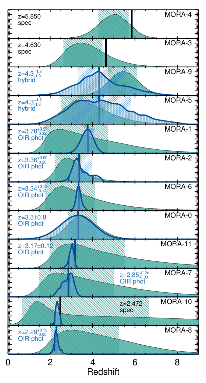
From the most to least reliable, two (2/11=18%) have spectroscopic redshifts, seven (7/11$\approx$64%) have OIR photometric redshifts, and two (2/11$\approx$18%) have hybrid FIR/mm and OIR photometric redshift constraints. It is somewhat interesting to note that the two spectroscopic redshifts are the highest redshift sources in the sample. Figure 4 shows the redshift constraints for each source (including MORA-10) in order of increasing redshift from bottom to top and how consistent existing constraints are with FIR/mm derived redshifts from the MMpz tool described in Casey (2020). The millimeter photometric redshifts serve as a sanity check on the tighter constraints given by other methods.

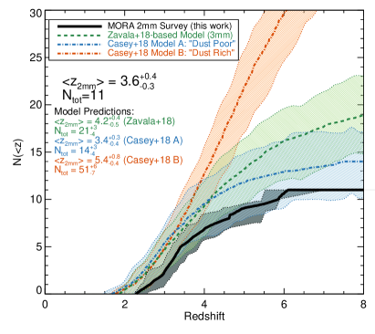
Figure 5 shows the cumulative redshift distribution for the entire sample in two panels. Given the heterogeneous constraints, each source’s probability density distribution in $z$ is coadded and shown as a cumulative distribution function (CDF) to make clear the relative fraction of the sample below or above a certain redshift threshold. Accounting for the uncertainties in the individual redshift constraints through Monte Carlo draws from the CDF, we measure the median redshift of the sample as $\langle z_{\rm 2mm}\rangle=3.6^{+0.4}_{-0.3}$. The variance in the redshift CDF is shown in gray and encompasses a 68% ($\pm 1\sigma$) minimum confidence interval. We find that 77$\pm$11% of the distribution lies at $z>3$ and 38$\pm$12% lies at $z>4$.

The median redshift of 2 mm-selected galaxies has been measured twice before in the literature, using the GISMO instrument on the single-dish IRAM 30 m telescope. Staguhn et al. (2014) measure a median redshift of $\langle z_{\rm 2mm}\rangle=2.9\pm 0.9$ for sources in the GISMO Deep Field in GOODS-N while Magnelli et al. (2019) measure a median redshift of $z\sim 4$, though only for five sources and four sources respectively with S/N$>$4. Both are in agreement with our measured median redshift of $\langle z_{\rm 2mm}\rangle=3.6^{+0.4}_{-0.3}$.

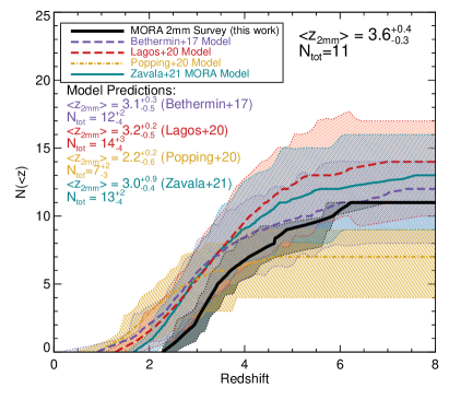
Figure 5 also shows the predicted cumulative redshift distributions for the MORA dataset from several models in the literature, described in § 4. For all models, we have generated the cumulative redshift distribution by sampling simulations over the 184 arcmin² area of the MORA survey. Some of the models have been simulated over larger areas (e.g. Shark, SIDES, and UniverseMachine) while the Casey et. al. and Zavala et. al. empirical models have multiple realizations the same size of the MORA survey. Sources in each model dataset then have an RMS noise assigned to them following the heterogeneous distribution of RMS noise in the MORA maps to best mimic the data. We retain simulated sources that were detected at or above 5$\sigma$ significance. Sources in these simulations are assumed to be point sources, as the probability of them being spatially resolved on scales larger than 1$\farcs$5$\approx$10 kpc is unlikely at these redshifts. This procedure is repeated 1000 times to constrain the uncertainties in the total number of selected sources and their redshift distribution.

The predictions of the Casey et al. (2018b) models A and B, as well as the Zavala et al. (2018a) model, are shown in the left panel of Figure 5. All are an overestimate of the number of sources in the true data, though the redshift distribution for the model A from Casey et al. does agree with our data within uncertainties. The right panel of Figure 5 shows four models, one of which is the updated empirical model from our accompanying paper, Z21. Z21 uses number counts from the MORA survey, alongside 1.2 mm number counts from ASPECS and 3 mm number counts to derive constraints on the high-$z$ IRLF, even in the absence of direct redshift measurements of individual galaxies. Thus it is important to emphasize that the predicted redshift distribution from Z21 constitutes an independent prediction, despite the use of MORA number counts to generate the model constraints.

Also shown on the right side of Figure 5 are the results from the three semi-empirical models grounded in cosmological simulations: SIDES (Bethermin et al., 2017), Shark (Lagos et al., 2020), and UniverseMachine (Popping et al., 2020). All models, with exception of the Popping et al. model which is only in slight tension, accurately predict the number of sources to be found in MORA within uncertainties due to cosmic variance. Similarly, their redshift distributions are also in broad agreement. Nevertheless, within the uncertainties on the redshift distributions, there is a systematic offset where most models predict median redshifts of $\langle z_{\rm 2mm}\rangle=2.2-3.2$ versus the observed $\langle z_{\rm 2mm}\rangle=3.6$. The Shark model comes closest to the measured median redshift, though we note the SIDES model has a more prominent high-redshift tail to its distribution similar to the MORA distribution. Only further data can reduce the uncertainties on the redshift distribution and discriminate between these models.

In summary, comparing the measured redshift distribution and number counts of our MORA results with models suggests that, indeed, the prevalence of dusty star-forming galaxies beyond $z\lower 2.15277pt\hbox{$\;\buildrel>\over{\sim}\;$}5$ is inherently low. This is well aligned with predictions from cosmological simulations, which fundamentally limit the build up of massive star-forming galaxies in the first $\sim$2 Gyr of the Universe’s history directly from the volume density of massive halos at that epoch.

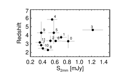
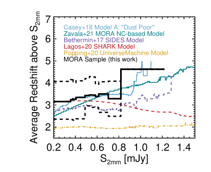
Despite this verification of models, there are still subtleties to these measurements worth exploring that could help refine early Universe DSFG volume densities further. For example, Figure 6 shows the relationship between 2 mm flux density and redshift for the MORA sample and model predictions. The Popping et al. (2020) model predicts a low average redshift for 2 mm-luminous sample that does not vary as a function of flux density. While SIDES and Shark accurately predict the redshift distribution and source density in the MORA map, they offer different predictions of which sources are most likely to sit at the highest redshifts; in other words, while SIDES predicts sources to sit at higher redshifts with brighter 2 mm flux density, Shark predicts that the average redshift for bright ($S_{\rm 2mm}\lower 2.15277pt\hbox{$\;\buildrel>\over{\sim}\;$}0.5$ mJy) 2 mm sources is relatively low compared to faint ($S_{\rm 2mm}\lower 2.15277pt\hbox{$\;\buildrel<\over{\sim}\;$}0.5$ mJy) sources. Our data – though limited severely by the small sample size – suggest that brighter sources tend to sit at higher redshifts (see also Koprowski et al., 2017). This is also in line with the predictions of both the Casey et al. (2018b) Model A and Z21 adjusted number counts-based MORA model, both of which show the highest average redshift for $S_{\rm 2\,mm}\lower 2.15277pt\hbox{$\;\buildrel>\over{\sim}\;$}1$ mJy sources.

The origins of these second order discrepancies between model predictions and data will inevitably require larger samples of 2 mm galaxies identified over wider areas. Nevertheless, we discuss possible origins of such discrepancies (and other potential degeneracies in our conclusions) later in § 6.5; possible causes include evolution in the faint-end slope of the IRLF, possible evolution of galaxies’ dust emissivity spectral indices, or galaxies’ bulk luminosity-weighted dust temperatures.

Figure 6: Top: 2 mm flux density against best redshift constraints for the MORA Sample; sources are labeled by their IDs. Bottom: the cumulative median redshift of the MORA sample above a given 2 mm flux density (thick black line, dashed lines enclose the inner 68^th-percentile). The median redshifts of five models are overplotted for comparison: the SIDES model from Bethermin et al. (2017) in purple (dashed line), the SHARK model from Lagos et al. (2020) in red (dashed line), the UniverseMachine model from Popping et al. (2020) in yellow (dot-dashed line), the dust-poor model from Casey et al. (2018b) in light blue (solid), and the Z21 model in teal (solid). The dearth of sources $>$1 mJy in this dataset limit our ability to distinguish between models, with exception of the Popping et al. (2020) model that underestimates the redshifts of 2 mm-selected galaxies of all flux densities.

5.2 Direct SED fits using redshift priors

We fit the FIR through millimeter spectral energy distributions of the 2 mm-detected sample using a modified blackbody plus a mid-infrared powerlaw; this procedure is a modified version of the fitting technique described in Casey (2012) and will be described in full in a forthcoming paper (Drew et. al., in preparation). The difference with the Casey (2012) analytical approximation is that the blackbody and mid-infrared powerlaw are added together as a piecewise function (where the mid-infrared powerlaw is joined at the point where the slope of the blackbody is equal to the powerlaw index $\alpha_{\rm MIR}$). The functional form of the fit used is:

$$S_{\nu}(\lambda)=\left\{\begin{array}[]{lr}N_{\rm pl}\lambda^{\alpha}&:\lambda\ |\ \frac{\partial\log S_{\nu}}{\partial\log\lambda}>\alpha\\ N_{\rm bb}\frac{(1-e^{-(\lambda_{0}/\lambda)^{\beta}})\lambda^{-3}}{e^{hc/\lambda kT}-1}&:\lambda\ |\ \frac{\partial\log S_{\nu}}{\partial\log\lambda}\leq\alpha\\ \end{array}\right.$$ (1)

Here $\lambda$ is the rest-frame wavelength, $T$ the modeled dust temperature, $\lambda_{0}$ the wavelength where the dust opacity is $\tau=1$, $\alpha$ is the slope of the mid-infrared powerlaw, and $\beta$ is the observed integrated emissivity spectral index. $N_{\rm pl}$ and $N_{\rm bb}$ are normalization constants whose value is tied to one another such that the SED is contiguous at the point of transition, i.e. where $\partial\log S_{\nu}/\partial\log\lambda=\alpha$. Both $N_{\rm pl}$ and $N_{\rm bb}$ are tied to L_IR, defined as the integral of the SED in $S_{\nu}$ between 8–1000 $\mu$m.

We adopt the general opacity model for all SEDs; for lack of direct constraints on the dust opacity in these systems, we adopt $\lambda_{0}=200$ $\mu$m. This is broadly consistent with what is seen in high-L_IR systems where $\lambda_{0}$ can be measured (e.g. Conley et al., 2011; Spilker et al., 2016); even if this presumption is incorrect in the case of these systems, the exact adopted value does not impact the results of this work. Specifically, it only impacts the functional relationship between $T$ and $\lambda_{\rm peak}$, where the latter quantity is insensitive to choice of $\lambda_{0}$; for example, Cortzen et al. (2020) show that the measured dust temperature for GN20 may vary by 20 K depending on the adopted $\lambda_{0}$, whereas the measured $\lambda_{\rm peak}$ remains unimpacted. So while it is known there are degeneracies in measured quantities $\beta$, $T$, and $\lambda_{0}$ that cannot be resolved with the limited data we have on this sample in full, it is worth emphasizing that measurement of $\lambda_{\rm peak}$ is independent and not sensitive to choice of opacity model. For the purposes of SED fitting, the photometric points are allocated an additional 10% calibration error, representing the degree to which the absolute value of the flux density across the (sub)millimeter regime is known.

Figure 7: An illustrative example of the two-dimensional joint posterior distributions for the IR SED fit to source MORA-2. The parameters fit are redshift $z$, the mid-infrared powerlaw slope $\alpha$, the emissivity spectral index $\beta$, the IR luminosity $L_{\rm IR}$, and the rest-frame peak wavelength $\lambda_{\rm peak}$. MORA-2 shows strong covariance between $z$, $L_{\rm IR}$, and $\lambda_{\rm peak}$. The resulting best-fit SED for MORA-2 is shown in Figure 8.

We converge on best-fit SEDs using a Markov Chain Monte Carlo routine. In all cases, we use the best available redshift probability distribution as a prior. Each SED is handled individually, whereby the choice to fix a variable or let it vary depends on the degree of photometric constraints relevant to each variable; for example, $\alpha_{\rm MIR}$ is fixed to $\alpha_{\rm MIR}=4$ if there are no detections at rest-frame mid-infrared wavelengths, and $\beta$ is fixed to $\beta=1.8$ (Planck Collaboration et al., 2011) if there are no more than 2-3 photometric points on the Rayleigh-Jeans tail of the blackbody emission in the millimeter regime. The choice of fixed $\alpha_{\rm MIR}=4$ is motivated by fits to lower redshift DSFGs with constrained mid-IR emission (e.g. at $z\sim 2$; Pope et al., 2008), while the choice of $\beta=1.8$ is motivated by well-constrained Rayleigh-Jeans emission in similar systems (e.g. Scoville et al., 2016). The free parameters for our least-constrained SED (MORA-9) are redshift, L_IR, and $\lambda_{\rm peak}$ (where both $\alpha_{\rm MIR}$ and $\beta$, the emissivity spectral index have been fixed). In contrast, the best-fit SEDs constrain up to five free parameters: $z$, L_IR, $\lambda_{\rm peak}$, $\alpha_{\rm MIR}$, and $\beta$.

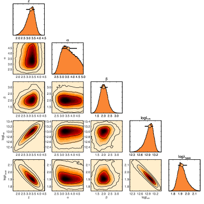
A graphical representation of the two-dimensional posterior distributions for each variable are shown in Figure 7 for MORA-2.

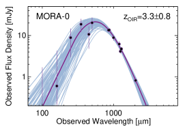
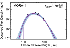
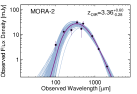
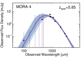
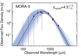
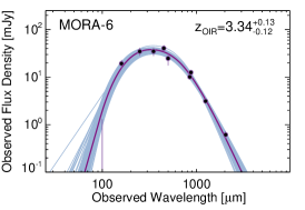
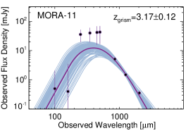
Figure 8 shows the resulting SED fits against measured source photometry. We see a variety of SED shapes presented here, from sources with prominent mid-infrared powerlaws to quite steep Rayleigh-Jeans tails ($\beta>2$). The uncertainties are illustrated by the range of accepted MCMC trial SED solutions, shown as light blue curves in Figure 8. Extracted fit characteristics are given in Table 2.

Figure 8: The best-fit dust SEDs for the $>$5$\sigma$ 2 mm-detected sample; SEDs are fit as a modified blackbody joined with a mid-infrared powerlaw. The modified blackbody fixes the opacity such that $\tau=1$ at $\lambda_{0}=$ 200 $\mu$m near the intrinsic peak of the dust SED; this assumption is not meant to be physically interpreted, but is rather fixed for convenience since our data cannot independently constrain $\lambda_{0}$. Fixing $\lambda_{0}$ has no impact on the measured $\lambda_{\rm peak}$. Four of these sources are detected at 100–160$\mu$m with Herschel-PACS, leading to a more prominent mid-infrared component than those that lack rest-frame mid-infrared detections. The uncertainty of the fit is shown via the light blue SED fits, drawn randomly from the successful MCMC trials. Sources without rest-frame mid-infrared data have fixed mid-infrared powerlaw slopes of $\alpha_{\rm MIR}\equiv 4$ and MORA-9, the only source with limited photometry on the Rayleigh-Jeans tail, has a fixed $\beta\equiv 1.8$. Measured SED characteristics are given in Table 2 and the sources’ photometry is given in Table Mapping Obscuration to Reionization with ALMA (MORA): 2 mm Efficiently Selects the Highest-Redshift Obscured Galaxies.

Table 2: Measured Physical Characteristics of the 2 mm-Detected Sample

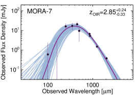
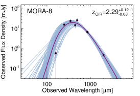
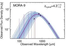
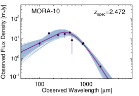
Name	$z$	$z$-Type	LIR	SFR	$\lambda_{\rm peak}$	$\beta$	$\alpha_{\rm MIR}$	Mdust	M⋆
			[ L⊙]	[ M⊙ yr-1]	[$\mu$m]			[ M⊙]	[ M⊙]
MORA-0	$3.3\pm 0.8$	OIR	(4.7${}^{+1.6}_{-1.0}$)$\times 10^{12}$	690${}^{+230}_{-150}$	133${}^{+15}_{-12}$	2.3${}^{+0.4}_{-0.1}$	3.6${}^{+1.1}_{-0.7}$	($1.4^{+0.5}_{-0.4}$)$\times 10^{9}$	(2.2${}^{+0.8}_{-0.8}$)$\times 10^{10}$
MORA-1	3.78${}^{+0.27}_{-0.32}$	OIR	(2.0$\pm 0.3$)$\times 10^{13}$	3000${}^{+500}_{-400}$	68$\pm$4	2.4${}^{+0.2}_{-0.4}$	5.2${}^{+1.2}_{-1.6}$	($3.6^{+1.6}_{-1.3}$)$\times 10^{8}$	(5.8${}^{+1.5}_{-1.9}$)$\times 10^{10}$
MORA-2	3.36${}^{+0.60}_{-0.28}$	OIR	($9.7^{+4.7}_{-2.7}$)$\times 10^{12}$	1400${}^{+700}_{-400}$	84${}^{+11}_{-12}$	2.0$\pm$0.3	5.6${}^{+1.8}_{-2.9}$	($6.0^{+2.2}_{-2.3}$)$\times 10^{8}$	(1.4${}^{+0.4}_{-0.3}$)$\times 10^{11}$
MORA-3	4.63	spec	(1.17${}^{+0.18}_{-0.16}$)$\times 10^{13}$	1730${}^{+270}_{-240}$	85${}^{+4}_{-5}$	3.11${}^{+0.15}_{-0.26}$	4.4${}^{+1.3}_{-1.1}$	$2.1^{+0.5}_{-0.6}$)$\times 10^{8}$	…
MORA-4	5.85	spec	(3.6${}^{+1.1}_{-0.9}$)$\times 10^{12}$	530${}^{+160}_{-130}$	96${}^{+12}_{-11}$	2.1${}^{+0.1}_{-0.3}$	$\equiv 4$	($6.1^{+1.7}_{-0.7}$)$\times 10^{8}$	(3.2${}^{+1.0}_{-1.5}$)$\times 10^{9}$
MORA-5	4.3${}^{+1.5}_{-1.3}$	hybrid	(4.1${}^{+2.7}_{-1.8}$)$\times 10^{12}$	610${}^{+390}_{-270}$	99$\pm$21	2.2${}^{+0.3}_{-0.5}$	$\equiv 4$	($6.2^{+4.2}_{-3.0}$)$\times 10^{8}$	(1.5${}^{+1.0}_{-0.7}$)$\times 10^{11}$
MORA-6	3.34${}^{+0.13}_{-0.12}$	OIR	(1.43${}^{+0.21}_{-0.18}$)$\times 10^{13}$	2120${}^{+310}_{-260}$	80$\pm$4	2.4${}^{+0.2}_{-0.3}$	7$\pm$2	($5.2^{+1.1}_{-2.0}$)$\times 10^{8}$	(7.0${}^{+1.7}_{-1.4}$)$\times 10^{10}$
MORA-7	2.85${}^{+0.24}_{-0.33}$	OIR	(3.5${}^{+1.5}_{-0.9}$)$\times 10^{12}$	510${}^{+220}_{-130}$	105$\pm$13	2.2${}^{+0.4}_{-0.3}$	6${}^{+3}_{-1}$	($4.4^{+1.6}_{-1.6}$)$\times 10^{8}$	(2.5${}^{+0.5}_{-0.5}$)$\times 10^{11}$
MORA-8	2.29${}^{+0.12}_{-0.08}$	OIR	(2.2$\pm$0.5)$\times 10^{12}$	330${}^{+70}_{-70}$	131${}^{+12}_{-10}$	1.8${}^{+0.3}_{-0.2}$	6.6${}^{+2.0}_{-2.2}$	($1.0^{+0.4}_{-0.2}$)$\times 10^{9}$	(1.1${}^{+0.2}_{-0.3}$)$\times 10^{11}$
MORA-9	4.3${}^{+1.3}_{-1.0}$	hybrid	(1.2${}^{+1.0}_{-0.4}$)$\times 10^{12}$	180${}^{+150}_{-60}$	123${}^{+26}_{-23}$	$\equiv 1.8$	$\equiv 4$	($8.2^{+5.1}_{-3.8}$)$\times 10^{8}$	(4.1${}^{+1.8}_{-1.4}$)$\times 10^{10}$
MORA-10	2.472	spec	(1.1${}^{+0.1}_{-0.1}$)$\times 10^{13}$	1570${}^{+160}_{-130}$	102${}^{+10}_{-13}$	1.7${}^{+0.4}_{-0.2}$	1.3${}^{+0.15}_{-0.14}$	($7.1^{+2.2}_{-2.3}$)$\times 10^{8}$	(7.3${}^{+2.0}_{-2.0}$)$\times 10^{10}$
MORA-11	3.17$\pm$0.05	OIR	(3.4${}^{+1.7}_{-1.1}$)$\times 10^{12}$	500${}^{+250}_{-170}$	99${}^{+13}_{-14}$	2.1${}^{+0.4}_{-0.4}$	$\equiv 4$	($3.5^{+2.5}_{-0.9}$)$\times 10^{8}$	(1.7${}^{+0.5}_{-0.3}$)$\times 10^{11}$

Table Notes. Derived physical properties of the 2 mm-detected MORA Sample. Variables which have been fixed are denoted with $\equiv$ notation. Estimates for ISM masses (not given in this table) can be obtained by multiplying the dust masses in this table by a factor of 125 (Rémy-Ruyer et al., 2014). A stellar mass estimate is not available for MORA-3 (a.k.a. AzTEC-2) due to blending of near-infrared imaging with foreground galaxies. All uncertainties in this table indicate the inner 68% minimum credible interval of posterior distributions.

Figure 9: The distribution of the 2 mm-detected sample in derived physical parameter space. Sources are color coded by the origins of their their redshift constraints: gray (spectroscopic), blue (OIR photometric) and teal (hybrid OIR/mm photometric). Contours denote sources’ 1 and 2$\sigma$ confidence intervals for the measured parameters, highlighting parameter covariance for the given set of photometry. Regions of the planes inaccessible to the MORA survey are shaded in gray in the first three panels: the cutoffs depend precisely on parameters of the SED fit. For example, in the L_IR$-z$ plane (top left), the gray curves trace out the detection limit of a source detected at 5$\sigma$ (1$\sigma$=70$\mu$Jy at 2 mm) with $\lambda_{\rm peak}$$\,\equiv\,100$$\mu$m and $\beta=1.8$, $\beta=2.2$ and $\beta=2.6$ (with $\beta=2.6$ corresponding to the flattest curve). In the M_ISM$-z$ plane (top right) the lower detection threshold corresponds to fits with $\beta=1.8-2.6$ (where the steepest curve corresponds to $\beta=2.6$). The light purple shaded regions in the M_ISM$-z$ plane also shows the theoretical maximum M_ISM mass limit as a function of redshift based on the Harrison & Hotchkiss (2013) halo mass survey estimator; the halo mass is scaled down to M_ISM by a factor of 20. The L_IR-$\lambda_{\rm peak}$ plane (bottom left) shows the aggregate, non-evolving L_IR-$\lambda_{\rm peak}$ relation from Casey et al. (2018b) (gray line with dashed lines enclosing 1$\sigma$ and 2$\sigma$ scatter) and agreement with the MORA sample SEDs. The gray region marks the detection limit for a $z=3$ system (the curves shift in L_IR with $z$ following the gray curves in the L_IR-$z$ panel). The distribution of sources’ emissivity spectral indexes ($\beta$) is shown against redshift (bottom right) with the canonical value of $\beta=1.8$ marked with the black dashed line. No evidence for redshift evolution of $\beta$ is seen in this (small) sample; the average value is $\langle\beta\rangle=2.2^{+0.5}_{-0.4}$.

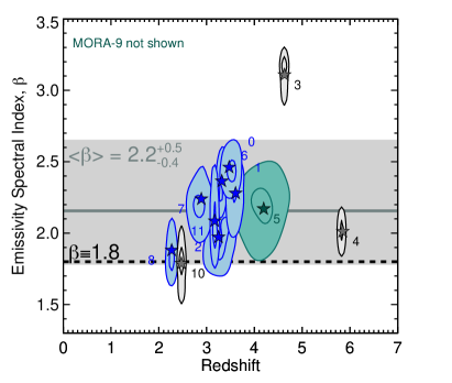
5.3 Distribution in L_IR, $\lambda_{\rm peak}$, $M_{\rm ISM}$, and $\beta$

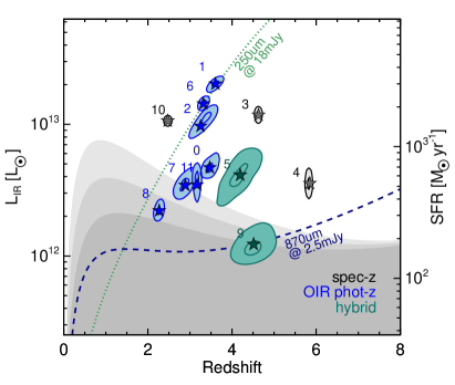
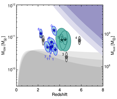
Figure 9 shows the distribution of the full sample of twelve galaxies in L_IR, $\lambda_{\rm peak}$, $M_{\rm ISM}$, and $\beta$, demonstrating the relative heterogeneous nature of the sample. Sources are color coded by quality of their redshift constraints, and contours denote 1–2$\sigma$ confidence intervals in the given parameter space.

The dynamic range in MORA sources’ IR luminosities is about a factor of $\sim$25, from the most extreme, MORA-1, topping 2$\times 10^{13}$  L_⊙ to the least extreme, MORA-9, $\sim$9$\times 10^{11}$  L_⊙ (the corresponding star-formation rates range from 140–3100  M_⊙ yr^-1). Given the selection of these sources on the Rayleigh-Jeans tail of dust blackbody emission at 2 mm, the dynamic range in ISM masses is much more narrow, mirroring the somewhat narrow dynamic range in 2 mm flux densities (both a factor of $\sim$3). The second panel of Figure 9 shows the measured ISM masses of the sample, scaled up by a factor of 125 from SED-inferred dust mass (to account for the total mass of gas in the ISM), which is consistent with the expected gas-to-dust ratio for near solar metallicity galaxies (Rémy-Ruyer et al., 2014). Note that a maximum ISM mass, as a function of redshift, is set in our survey by the size of the survey itself given a $\Lambda$CDM Universe (purple shaded regions in the $M_{\rm ISM}-z$ panel of Figure 9, at 1–3$\sigma$ confidence intervals); this peak is determined by the maximum halo mass as a function of redshift and survey volume from Harrison & Hotchkiss (2013), using an ISM-to-halo mass ratio of 1/20 (as is done in Marrone et al., 2018).

While the nominal 2 mm detection limit in L_IR with redshift follows the strong negative K-correction (and thus is more sensitive to sources at $z\lower 2.15277pt\hbox{$\;\buildrel>\over{\sim}\;$}3$ than $z=1-2$; denoted by gray bands), the detection limit in $M_{\rm ISM}$ is approximately flat. These detection curves are not absolute limits as they are sensitive both to galaxies’ luminosity-weighted dust temperature and the emissivity spectral index. For example, a galaxy of ISM mass $\sim 2\times 10^{10}\,$ M_⊙ at $z=4$ may only be detectable in MORA if its emissivity spectral index is lower than $\beta\lower 2.15277pt\hbox{$\;\buildrel<\over{\sim}\;$}2.2$, or a $\sim 2\times 10^{12}$  L_⊙ system at $z=3$ may only be detectable in MORA if its rest-frame peak wavelength falls within $95\lower 2.15277pt\hbox{$\;\buildrel<\over{\sim}\;$}\lambda_{\rm peak}\lower 2.15277pt\hbox{$\;\buildrel<\over{\sim}\;$}175$ $\mu$m.

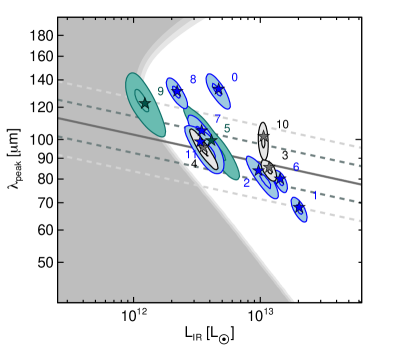
The galaxies’ distribution in rest-frame peak wavelength, $\lambda_{\rm peak}$ (a proxy for the luminosity-weighted dust temperature) is shown in the third panel of Figure 9 relative to the aggregate DSFG population fit found in Casey et al. (2018b), with intrinsic scatter of 1–2$\sigma$ shown. The MORA galaxies are largely in agreement with the global DSFG trend, with two sources appearing to be somewhat anomalously cold (MORA-0 and MORA-8). For a sample this small, we would only expect at most one source to sit $>$2$\sigma$ offset from the global trend given that galaxies are distributed in a Gaussian about the mean L_IR-$\lambda_{\rm peak}$ relation. The cold SED for MORA-0 is somewhat uncertain given the significant uncertainty on the source’s redshift; if this source is indeed at the higher redshift end of its redshift PDF, its SED would be better aligned with the overall trend for DSFGs’ peak wavelengths. Nevertheless, it is worth highlighting that 2 mm selection itself may skew the temperatures of the sample a bit cold; the gray region in the third panel of Figure 9 shows the parameter space beyond reach of the MORA survey at a fixed redshift of $z=3$. If the survey had a flat selection in L_IR around $\sim$3$\times 10^{12}$  L_⊙, MORA-9 and MORA-8 may not have made the cut, as they’re the least luminous sources in the sample; excluding them, only one source, MORA-0, is anomalously cold, in line with expectation for a sample this size.

The average value of the emissivity spectral index of MORA galaxies in the sample is $\langle\beta\rangle=2.2^{+0.5}_{-0.4}$, which is skewed toward higher values than are often typically assumed for galaxies in the absence of direct measurements. The fact that the MORA sample is 2 mm selected would potentially impact the average measured $\beta$. However, one would assume it would do so in the opposite sense, by more efficiently identifying sources with shallower emissivity spectral indices (or $\beta<1.8$) due to higher relative 2 mm flux densities for a given L_IR. While nominally substantial heating from the CMB at high-$z$ ($z\lower 2.15277pt\hbox{$\;\buildrel>\over{\sim}\;$}5$) could effectively steepen the Rayleigh-Jeans slope (and artificially increase $\beta$ as discussed in Jin et al. 2019), here we account for CMB heating directly and find its effect negligible. There is no evidence in the MORA sample of evolution in $\beta$; because the sample size is relatively small, the mean could also not be precisely constrained. Our interpretation of $\beta$, relative to other literature samples and other DSFGs falling within the MORA footprint, is offered in § 6.3.

Figure 10: Placement of MORA 2mm-selected sample in the galaxy M_⋆-SFR relation, or galaxy “main sequence.” Colored lines and $\pm$0.3 dex shaded regions represent the $z=2$ (purple), $z=3$ (blue), $z=4$ (green), $z=5$ (orange), and $z=6$ (red) average relations from Speagle et al. (2014). The dashed navy line represents the lower envelope for starbursts as defined in Caputi et al. (2017, 2021). Galaxies are labeled by their MORA IDs, and color coded according to the $\Delta z=1$ interval in which they most likely sit (e.g. MORA-0 with $z_{\rm OIR}=3.3$ is blue to denote it sits at $3<z<4$). All sources except MORA-3 (a.k.a. AzTEC-2) have stellar mass estimates, and thus that source’s SFR is noted as a horizontal green band with unconstrained stellar mass; MORA-3 lacks an estimate due to severe blending of IRAC photometry with foreground galaxies. With respect to the main sequence, the MORA sample splits roughly in half: 5/12 galaxies sitting on the galaxy main sequence while 7/12 are significantly elevated, the most extreme of which is MORA-4 (a.k.a. MAMBO-9 Casey et al., 2019) which is (likely) the highest redshift source of the sample.

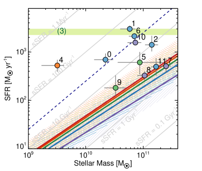
5.4 Stellar masses and the SFR-M_⋆ relation

Stellar masses are derived using the suite of OIR COSMOS photometric constraints available for each source (Weaver, Kauffmann et. al., submitted). While Weaver et. al. use LePhare (Arnouts et al., 2002; Ilbert et al., 2006) and a range of 19 stellar population templates from Bruzual & Charlot (2003), we only make use of their posterior redshift probability density distributions for the subset of MORA sources detected in the COSMOS2020 catalog. We choose to remodel the galaxies’ stellar populations using a wider range of templates inclusive of extreme starbursts. This refitting is carried out using the Magphys energy balance code (da Cunha et al., 2008) and Bruzual & Charlot (2003) stellar population synthesis templates and an updated, wider range of star formation histories compatible with DSFGs (da Cunha et al., 2015). Redshift uncertainties are accounted for by iteratively sampling the sources’ redshift PDFs; we find that stellar masses are largely insensitive to redshift uncertainties. Similarly, the stellar masses derived from Magphys show no systematic offset with those reported by Weaver et. al., though significant uncertainty on all derived stellar masses remains.

There are a few exceptions where our technique is approached with even more caution: MORA-3, MORA-4, MORA-5, and MORA-9. The first, MORA-3 (a.k.a. AzTEC-2), lacks any OIR counterpart shortward of 2.2 $\mu$m and at longer wavelengths is spatially confused with foreground galaxies, thus rendering any stellar mass constraint impossible without future spatially-resolved JWST observations. Though the Magphys predicted stellar mass for MORA-4 (a.k.a. MAMBO-9) is reasonable on a standalone basis, Casey et al. (2019) present a detailed argument as to why it is most likely an overestimate given the measured gas mass and implied halo mass. Therein they provide an alternate stellar mass estimate of MAMBO-9 following the methodology outlined in Finkelstein et al. (2015), which uses stellar population modeling plus the contribution from nebular emission. Note that the necessity of this approach is thought to be unique to that source, given that MAMBO-9 is likely the highest redshift source in the sample and intrinsically massive, thus the survey volume itself sets an upper limit to its mass.

The last two exceptions to the standard Magphys stellar mass-fitting approach are sources MORA-5 and MORA-9, which are the two OIR-dark sources explored in more detail in Manning et. al., as they lack good redshift constraints. Their stellar masses are fit using the Magphys+photo-z code (Battisti et al., 2019), which is a further update to Magphys allowing for redshift uncertainty; this was deemed necessary in the case of MORA-5 and MORA-9 in particular, given the significant uncertainties on both sources’ photometric redshifts. The resulting best-fit stellar masses are reported in Table 2.

Figure 10 shows the distribution of the MORA sample in the galaxy SFR–M_⋆ plane relative to observed trends for the bulk galaxy population at various redshifts (i.e. the galaxy “main sequence”). The trend lines are drawn from Speagle et al. (2014) at fixed redshifts and sources are color coded by redshift, and the dashed navy line demarcates the lower envelope for “starbursts” (sSFR$\,>\,$25 Gyr^-1; Caputi et al., 2017, 2021). What we observe is a rather heterogeneous sample: 7/12 (58%) MORA-selected sources are significantly elevated above the ‘main sequence’ with specific star formation rates in excess of ${\rm sSFR}\,>\,10\,{\rm Gyr}^{-1}$ (with 5/12, 42% above the 25 Gyr^-1 threshold). The remaining 5/12 (42%) are embedded in the galaxy main sequence itself, with $1\,$Gyr${}^{-1}<{\rm sSFR}<10\,$Gyr^-1. There does not appear to be a strong correlation between sources’ redshifts and whether or not they have elevated sSFRs. The fact that the sample is somewhat heterogeneous in the SFR–M_⋆ plane is not surprising given that the 2 mm selection (and submillimeter selection more broadly) roughly corresponds to a SFR cut, modulo variation due to SED dust temperature and emissivity. Later in § 6.2 we discuss some of the implications of the sample’s measured stellar content in relation to the formation of the first massive quiescent galaxies.

With a median stellar mass of 7$\times 10^{10}\,$ M_⊙, we note that the median dust-to-stellar mass ratio in this sample is $M_{\rm dust}/M_{\star}=(7^{+30}_{-3})\times 10^{-3}$. This is nominally a bit higher than expected for DSFGs, though one would expect a 2 mm sample to be slightly biased in that regard, selecting more galaxies rich in dust per unit stellar mass than selection at shorter wavelengths.

5.5 2 mm Characteristics of Known (Sub)Millimeter Sources

Figure 11: The 870$\mu$m to 2 mm flux density ratio against redshift and in histogram for DSFGs from various samples. Left: The $S_{\rm 870}/S_{\rm 2000}$ ratio for DSFGs that have secure redshift constraints, including $>$5$\sigma$ MORA sources (dark gray points) and marginal MORA sources (light gray points); we have also overplotted two other samples of well-characterized DSFGs in the literature: the SPT (1.4 mm-selected) sample from Reuter et al. (2020), and the ALESS (870$\mu$m-selected) sample from da Cunha et al. (2021). Overlaid are tracks of specific SEDs with variable dust temperature ($\lambda_{\rm peak}=95$ $\mu$m or 125$\mu$m, solid vs. dashed) and variable emissivity spectral index ($\beta=$1.8, 2.2, or 2.6, in increasingly dark shades of orange, respectively). Right: Histograms of $S_{\rm 870}/S_{\rm 2000}$ for sources without redshifts that: have 870$\mu$m ALMA data (dark gray), sources with 870$\mu$m data only from SCUBA-2 (light gray), and the full distributions of the SPT sample (purple dot-dashed) and ALESS sample (dotted blue). Downward arrows mark the maximum color ratio that could correspond to a given value of $\beta$ at $z=2.5$; higher ratios are not allowed for the given $\beta$, as the ratio of flux densities only diminishes with redshift. Our data suggest a range of $\beta$ values apply to this sample, from some being fully consistent with the often-presumed value of $\beta=1.8$, to some being more consistent with steeper slopes, $\beta\approx 2.2-2.6$.

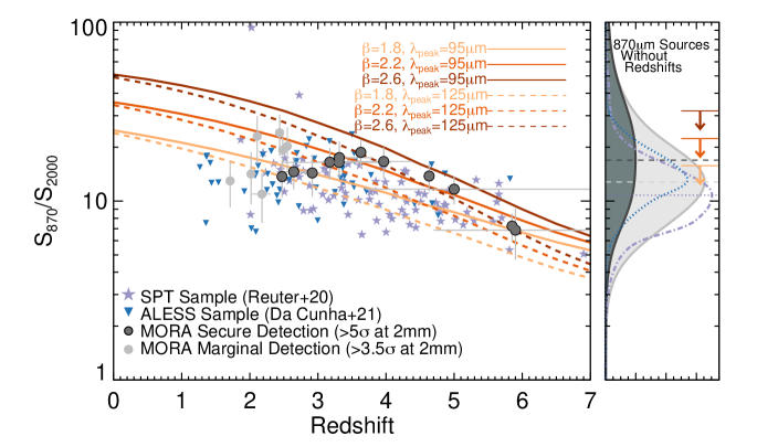
Here we analyze the 2 mm characteristics of known submillimeter sources in the MORA footprint, taken from the Simpson et al. (2019) deep SCUBA-2 850$\mu$m map. We select sources from that work detected above a signal-to-noise of 4, roughly corresponding to a flux threshold of $S_{\rm 850}\lower 2.15277pt\hbox{$\;\buildrel>\over{\sim}\;$}$2.3 mJy (i.e. ${\rm RMS}\approx 0.57$ mJy/beam), minimizing spurious detections at lower significance. Only 55/98 ($\approx$ 56%) sources have interferometric follow-up from ALMA other than our band 4 data, allowing identification of their precise astrometric positions in the MORA map. The remainder (43/98 $\approx$ 44%) lack precise position constraints and are not well known to better than the JCMT beam (14$\farcs$8). For those sources, we search for possible corresponding marginally-detected 2 mm sources by identifying the highest significance peak within the FWHM of the JCMT beam.

Out of 98 $>4\sigma$ SCUBA-2 sources overlapping with the main MORA mosaic, 17/98 (=17.3%) have 2 mm peaks detected at $>4\sigma$ (including the 12 sources in our 5$\sigma$ sample). This compares to 3.7% of randomly placed JCMT beam ‘apertures’ containing $>4\sigma$ sources. Most of this excess signal comes from our $>5\sigma$ sample. However, our data still show an excess between $4<\sigma<5$ significance with 5/86 (= 5.8%) found in total compared to the random ‘aperture’ rate of 3.7%. We find 56/98 (= 57$\pm$7%) SCUBA-2 sources have between $3<\sigma<4$ significance peaks in the 2 mm map, compared to 48$\pm$2% of randomly placed apertures. Of those sources with $3<\sigma<4$ 2 mm counterparts, the median 850$\mu$m flux density is 3.4 mJy, lower than the median for the $4<\sigma<5$ sample with 6.8 mJy. While the excess signal over random apertures is relatively low significance due to significant potential for contamination, it is still indicative of real 2 mm emission associated with these known 850$\mu$m sources.

Fifty-five of the 98 SCUBA-2 sources sitting in the MORA footprint have other ALMA continuum data covered by the archival A3COSMOS project (described in detail in Liu et al., 2018) and 45/55 have a confirmed ALMA counterpart detected at or above 3$\sigma$ in their corresponding archival ALMA data (of varying observed frequencies, most at 870$\mu$m or 1.2 mm); 7 of the 45 sources have two components or sources (separated by more than 1^′′) detected by ALMA within the JCMT beam (and 2/7 have one of their multiples detected at 2 mm at $>$5$\sigma$). The highest SNR 2 mm detection within the JCMT beam corresponds to the correct, independently-identified (single) ALMA counterpart in 24 of 45 cases ($\approx 53$%).

Out of the 98 sources, fifty-five also have some form of redshift constraint (derived independently from the mm photometry), ranging from spectroscopic confirmation in the millimeter or optical/near-infrared, or through an optical/near-infrared photometric redshift. These 55 sources with redshift constraints are not the same 55 with independent ALMA data; only 37 sources have both redshifts and secure ALMA counterparts.

Figure 11 shows the distribution of millimeter colors for the sample of known SCUBA-2 sources in the field, i.e. $S_{\rm 870}/S_{\rm 2000}$, or the ratio of ALMA measured 870$\mu$m flux density (or SCUBA-2 850$\mu$m) to 2 mm flux density as measured by MORA. Sources are split into those with redshift constraints (left panel) and those without (right panel). We also include several model tracks in color space as a function of dust temperature (or $\lambda_{\rm peak}$) and emissivity spectral index ($\beta$) as well as literature samples of DSFGs with well-constrained Rayleigh-Jeaons SEDs, like the SPT 1.4 mm-selected sample from Reuter et al. (2020) and the ALESS 870$\mu$m-selected sample from da Cunha et al. (2021).

While naively one might think this 870-to-2 mm color ratio indicative purely of $\beta$, the emissivity spectral index, given that both 870$\mu$m and 2 mm flux density measurements are likely to sit on the Rayleigh-Jeans tail of dust blackbody emission, the color ratio has both a temperature and redshift dependence that can result in significant deviation from expectation given a fixed value of $\beta$. For example, the approximation that the flux density on the Rayleigh-Jeans tail of a blackbody follows $S_{\nu}\propto\nu^{2+\beta}$ is often used, while in practice the SED only asymptotically approaches this at rest-frame wavelengths longward of rest-frame $\sim$2 mm. Even at moderate redshifts ($z\sim 1$), our observed bands probe shorter rest-frame wavelengths where this approximation no longer holds. This is why there is a redshift dependence on $S_{\rm 870}/S_{\rm 2000}$ at redshifts well below the point that either wavelength probes the peak of the SED. The temperature dependence may also be somewhat intuitive: at colder intrinsic temperatures, the evolution toward lower $S_{\rm 870}/S_{\rm 2000}$ ratios is steeper at lower redshifts, as the 870$\mu$m band more quickly probes the peak of the SED than it would for a source with a hotter SED.

We see that both MORA and literature DSFG samples roughly follow the model trend evolution of $S_{\rm 870}/S_{\rm 2000}$ with redshift; however, at higher redshifts, the $>$5$\sigma$ 2 mm sample (points enclosed in black circles) also suggest consistency with steeper values of $\beta$ than the nominal $\beta=1.8$. Figure 11 also marks the maximum color value (in $S_{\rm 870}/S_{\rm 2000}$) allowed for given fixed value of $\beta$, which is set by the measured color for $z=2.5$ systems (in other words, at all higher redshifts, the color will be substantially lower). Though there is a significant degeneracy between $S_{\rm 870}/S_{\rm 2000}$ color and redshift, $\beta$ and $\lambda_{\rm peak}$, as indicated by the tracks on the figure, it appears that many sources skew toward higher colors than would be allowable for $\beta=1.8$: both from the sample with redshift constraints and from the distribution of colors for sources without redshifts. This indicates that at least a subsample of the population likely skews toward steeper values of $\beta$. This is consistent with our finding for individual sources in the $>$5$\sigma$ 2 mm sample that have $\langle\beta\rangle=2.2$, described earlier in § 5.2. Further discussion of the implications of steeper values of $\beta$ are given in § 6.3.

6 Discussion

Prior to the MORA survey described herein, constraints on the prevalence of dust-obscured star forming galaxies beyond $z\lower 2.15277pt\hbox{$\;\buildrel>\over{\sim}\;$}3-4$ were relatively weak; refining the measurement of DSFGs’ number densities and characteristics during this epoch was the survey’s primary goal. Here we discuss the implications of our measurements, from the observed contribution of DSFGs to the cosmic SFRD beyond $z\lower 2.15277pt\hbox{$\;\buildrel>\over{\sim}\;$}3$, to the buildup of massive galaxies in the first few Gyr, and to the measured dust emissivity index in early-Universe DSFGs. We then present the limitations of the survey, particularly given the survey area and small sample size of detected sources, as well as various model degeneracies that could be broken with future millimeter-wavelength observational campaigns.

6.1 Contribution to the SFRD

The question of DSFGs’ contribution to the cosmic star-formation rate density at early times has been difficult to constrain. However, the MORA Survey’s design is meant to effectively filter out lower redshift DSFGs, enabling direct measurement of the obscured galaxy contribution to the SFRD. For example, the contrast between a “dust poor” universe (e.g. Koprowski et al., 2017; Dudzevičiūtė et al., 2020) and a “dust rich” universe (Rowan-Robinson et al., 2016; Gruppioni et al., 2020) would result in very different manifestations of the MORA dataset; the former predicts $\;\buildrel<\over{\sim}\;$15 sources with median redshift $z\sim 3.4$, and the latter predicts $\;\buildrel>\over{\sim}\;$50 sources with a median redshift of $z\sim 5.4$. So what does our dataset imply for the SFRD?

Figure 12: The contribution of 2 mm sources detected in the MORA Survey to the cosmic star formation rate density (black stars; open stars where incomplete at $z\lower 2.15277pt\hbox{$\;\buildrel<\over{\sim}\;$}3$). Our measurements are shown relative to the reported literature values from the Madau & Dickinson (2014) review (orange points indicating direct IR measurements, and blue points indicating rest-frame UV/optical measurements, corrected for dust attenuation). The results from our accompanying paper, Zavala et. al. (Z21), for the integrated IR/obscured component is shown as an orange, shaded band out to $z\sim 8$ including the impact of cosmic variance (the black stars do not). The Z21 band is inferred from a joint analysis of 1 mm, 2 mm and 3 mm number counts and the empirical model described in Casey et al. (2018b). We compare the contribution of this 2 mm-selected sample with the measured contribution from 870$\mu$m-selected sources from the AS2UDS Survey above 1 mJy (gray circles) in Dudzevičiūtė et al. (2020). The measurements in this paper (black stars) account directly and only for the eleven sources found above $>5\sigma$ in the MORA Survey, and do not represent an extrapolation of a fitted luminosity function; the uncertainties in sources’ redshifts and SFRs are accounted for. The dearth of sources at $z\lower 2.15277pt\hbox{$\;\buildrel<\over{\sim}\;$}3$ is a direct consequence of the 2 mm survey design, meant to efficiently ‘filter out’ the majority of DSFGs at $1\lower 2.15277pt\hbox{$\;\buildrel<\over{\sim}\;$}z\lower 2.15277pt\hbox{$\;\buildrel<\over{\sim}\;$}3$ that dominate cosmic star-formation at its peak.

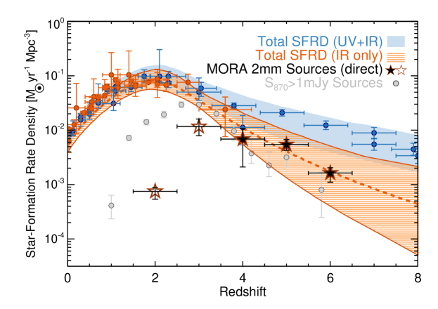
We provide direct estimates of the MORA sample’s contribution to cosmic star-formation in Figure 12. The SFRD contribution for this sample is estimated in the following way; first, we determine the area over which each of the 11 sources would be detectable in the MORA map above $>5\sigma$ significance. As a reminder, we exclude MORA-10 for its synchrotron component and MORA-12 as a likely false positive. Then we sample both the redshift and SFR probability density distributions for each source through Monte Carlo trials; this method accounts for their relative covariance. Sources’ SFRs are converted to a SFRD by dividing by the appropriate survey volume corresponding to the area over which a given source is accessible. A total SFRD, binned by $\Delta z=1$ intervals, is then measured for each Monte Carlo trial, and the average and 68% minimum confidence interval of all trials is used to infer the MORA source contribution to the SFRD, as shown in Figure 12. Though redshifts in our sample only nominally span $z=2.2-5.9$, our SFRD estimates span $z=1.5-6.5$ from the tails in the redshift PDFs for some of the less well-constrained sources.

Overall, we find the prevalence of $z<2$ sources and $z>6$ sources in this 2 mm-selected sample is quite low compared to the $2<z<6$ sample. Here our $z<3$ SFRD measurements are lower than measured from other DSFG samples due to 2 mm selection serving as an effective filter for $1<z<3$ DSFGs, thus those points are shown as open stars to contrast with filled stars at $z>3$, where the 2 mm sensitivity is more complete for $\;\buildrel>\over{\sim}\;$2$\times$10¹²  L_⊙ DSFGs, as shown in Figure 9.

The total contribution of MORA 2 mm-detected DSFGs at $3<z<6$ appears to be roughly $\sim$30% of the total cosmic SFRD at these epochs, shown as the blue band in Figure 12. Note that what is shown in Figure 12 represents a direct accounting for the $>5\sigma$ MORA-detected sample only, not an extrapolation from a luminosity function. This is clearly seen in the apparent deficit of the SFRD at $z<3$, where we know the MORA survey was designed to filter sources out.

Our accompanying paper, Z21, provides a detailed analysis on MORA constraints on the infrared luminosity function (IRLF) and the implied contribution of obscured galaxies to the SFRD out to $z\sim 7$. This is done using a joint analysis of 1 mm, 2 mm, and 3 mm number counts, plus our empirical model (described at length in Casey et al., 2018b, a; Zavala et al., 2018a) to measure the redshift evolution of the IRLF. In particular, the free parameters of the model are the evolution of $\Phi_{\star}$ beyond $z\sim 2$, the faint-end slope $\alpha_{\rm LF}$ (assumed not to evolve with redshift for simplicity), and the average emissivity spectral index of DSFGs $\beta$ (assumed not to evolve for simplicity). The data used to constrain the model are all aggregate (sub)mm number counts, with particular emphasis on 2 mm and 3 mm in their ability to capture the high-$z$ redshift evolution of $\Phi_{\star}$. Z21 finds that $\Phi_{\star}\propto(1+z)^{\psi_{2}}$, where $\psi_{2}=-6.5^{+0.8}_{-1.8}$, and the resulting total contribution of obscured emission to the SFRD is shown by the orange band in Figure 12.

What is of particular note in our SFRD estimate is that our direct accounting of MORA-detected galaxies agrees rather well with the best estimate of the integrated IRLF inferred by number counts. This effectively means that the sources found in our map are the only obscured sources to be found at these high redshifts, and there is not likely to be a population of fainter sources lurking just below the detection limit (or at least any population that contributes significantly to cosmic star-formation at those epochs). The same cannot be said of rest-frame ultraviolet luminosity functions (UVLF), for which there is often a significant discrepancy between the integrated SFRD contribution between directly detected galaxies and the inferred contribution from an extrapolation down the luminosity function (Finkelstein et al., 2015; Finkelstein, 2016). The key difference between the IRLF and UVLF is, of course, their faint-end slopes; while the UVLF has a steep faint-end slope, suggestive of a large population of low-mass, UV-luminous galaxies, the IRLF has a very shallow faint-end slope (see also González-López et al., 2020; Popping et al., 2020, for measurement of the faint-end slope of the IRLF from the ASPECS survey). This effect also manifests in most of the CIB having been resolved into individual, bright point sources (Béthermin et al., 2012). Our findings – agreement between direct accounting for MORA-detected sources to the SFRD and by integrating the extrapolated IRLF – are thus consistent with $\lower 2.15277pt\hbox{$\;\buildrel>\over{\sim}\;$}10^{12}\,$ L_⊙ sources being the dominant source of obscured emission. This is functionally equivalent to most dust luminosity living in massive galaxies, if indeed high-mass galaxies roughly correspond to high-luminosity galaxies.

Also of note in our SFRD estimates is the relative agreement between an estimate based solely on number counts (that from Z21) and our results here, that incorporate both sources’ inferred luminosities (thus SFRs) as well as redshift constraints. It is plausible that the additional redshift information introduced here would lead to some discrepancies with the Z21 model, either showing a flatter (or steeper) SFRD contribution with redshift, but the agreement of the Z21 model with these data holds. However, it should not be entirely surprising that the two agree so well across $3<z<6$ given the root assumption behind the Z21 model: that there are unlikely to be abrupt kinks or changes in the IRLF with redshift. While we nominally do not find any $z>6$ DSFGs in the MORA survey, we know they exist even if rare (Zavala et al., 2018a; Marrone et al., 2018). Measuring their volume density will require larger area 2 mm campaigns, discussed further in § 6.4.

We also draw comparison with the 870$\mu$m-selected DSFGs from the AS2UDS survey in Dudzevičiūtė et al. (2020), who present the characteristics of 870$\mu$m SCUBA-2-selected DSFGs across a 1 deg² area survey and followed up with ALMA. The contribution of sources above 1 mJy at 870$\mu$m are shown in Figure 12 as gray points. A direct comparison of the 870$\mu$m-selection vs. 2 mm selection technique is aligned with expectation: 870$\mu$m efficiently selects DSFGs above $z\lower 2.15277pt\hbox{$\;\buildrel>\over{\sim}\;$}1.5$, with a high-redshift tail extending to $z\sim 6$, while 2 mm selection is weighted towards the higher redshifts only ($z>3$). Both the AS2UDS and MORA results are well aligned with findings from the Shark model that predicts 2 mm-selected galaxies contribute between $\sim 15-28$% to cosmic star-formation at $3<z<6$ (Lagos et al., 2020).

Lastly, it is worth noting that our measurements are in disagreement with recent constraints on the $z>4$ IRLF from the ALPINE survey, who infer an integrated SFRD contribution from dust obscured sources a factor of $\sim$10 higher than found in this paper; ALPINE used serendipitous detections in very deep ALMA pointings of $z\sim 4-5$ galaxies (the primary goal being the measurement and characterization of galaxies’ [CII] characteristics) to place constraints on the high-$z$ IRLF (Gruppioni et al., 2020) and cosmic star-formation rate density more broadly (Loiacono et al., 2021; Khusanova et al., 2021). This discrepancy could be due to a bias in survey area used – whereby sources are physically associated with the ALPINE primary targets, even if that association is not directly known – or alternatively, could be due to increased cosmic variance in the relatively small area of the survey ($\sim$25 arcmin² vs. 184 arcmin² in MORA).

Recent findings from a similar higher-redshift line survey, the REBELS program, led to the discovery of two SFR$\sim$70  M_⊙ yr^-1 systems at $z\sim 7$ (Fudamoto et al., 2021), whose OIR emission is completely obscured. Fudamoto et al. estimate their volume density and contribution to the SFRD, attempting to correct for the bias introduced by the targeted survey approach. They predict a much higher contribution of lower IR luminosity ($\log$L_IR$\sim$11.5–12.2) sources to the obscured SFRD, of order the same contribution as we estimate exists for higher luminosity sources ($\log$L_IR$\;\buildrel>\over{\sim}\;$12.2). Indeed, the Z21 model would predict that such lower IR luminous sources ($\log$L_IR$\sim$11.5–12.2) would have an order of magnitude lower contribution to the SFRD than measured by Fudamoto et al.. The origin of this discrepancy is unclear and cannot be resolved without a more extensive census of the lower luminosity regime. Nevertheless, detection of such “OIR-dark” obscured galaxies within the Epoch of Reionization represents a significant leap, indicating that even modest SFR galaxies may indeed be dust rich at $z>7$.

Because ALPINE and REBELS are intrinsically targeted surveys and not blank field work, we omit their estimates from Figure 12 for clarity.

6.2 Progenitors of first Massive, Quiescent Galaxies?

An important consequence of our measurement of the prevalence of DSFGs at $z>3$ is their implications for the formation of the first massive quiescent galaxies, already well-established three billion years after the Big Bang (at $z=2$, placing the formation redshift of their stellar mass at $z>3$; e.g. Kriek et al., 2009; Toft et al., 2014; Schreiber et al., 2018a; Merlin et al., 2019; Marsan et al., 2020; Santini et al., 2021). Furthermore, the discovery of a substantial population of $M_{\star}\sim 10^{11}\,$ M_⊙ galaxies at $z\sim 4$ (Straatman et al., 2014; Marsan et al., 2020; Sherman et al., 2020; Valentino et al., 2020; Stevans et al., 2021) with a volume density of (1.8$\pm$0.7)$\times 10^{-5}$ Mpc^-3 requires a population of star-forming progenitors at $z\sim 5$ with SFRs $\sim$ 100  M_⊙ yr^-1. Though constraints on the quiescent population’s volume density are yet uncertain, recent observational works have constrained the number density to a few$\times 10^{-6}$ to $10^{-5}\,$Mpc^-3 (see recent compilation of quiescent galaxy number densities in Valentino et al., 2020). The population of DSFGs selected at 2 mm (or similarly, 3 mm, see Zavala et al., 2018a; Williams et al., 2019) are such star-forming systems; does their volume density, as a function of redshift, match the quiescent galaxy population? While not all DSFGs will quench in time to transition and become quiescent by $z\sim 3-3.5$, a comparison of their measured volume densities serves as a useful benchmark.

The raw volume density of MORA-detected galaxies (with a rough luminosity cut of $\lower 2.15277pt\hbox{$\;\buildrel>\over{\sim}\;$}2\times 10^{12}$  L_⊙ or 300  M_⊙ yr^-1) at $4<z<6$ is $\sim$(3.8${}^{+1.3}_{-0.7}$)$\times 10^{-6}$ Mpc^-3. This requires a correction for the DSFGs’ relatively short duty cycle, $\sim$100 Myr (Ivison et al., 2011; Bothwell et al., 2013; Swinbank et al., 2014), shorter than the period of the redshift interval over which the volume density is calculated ($\sim$600 Myr from $4<z<6$). The corrected volume density is $\sim$(2.2${}^{+0.8}_{-0.4}$)$\times 10^{-5}$ Mpc^-3. Note that this roughly agrees with other previous constraints on the $z>4$ DSFG volume density (e.g. da Cunha et al., 2015; Michałowski et al., 2017; Miettinen et al., 2017), though here the constraints are somewhat more precise. Note that it is, however, unclear if all DSFGs have universally short duty cycles, as the star formation histories of quiescent galaxies suggest some long DSFG lifetimes (e.g. Schreiber et al., 2018a; Forrest et al., 2020).

Within uncertainties, the volume density of MORA 2 mm-detected DSFGs is well aligned with constraints on $z\sim 3.5$ quiescent galaxies. Improved statistics from larger field 2 mm surveys will substantially reduce the uncertainty on the DSFG progenitor volume density at these epochs though there remains substantial relative uncertainty in the quiescent population. This may be due, in large part, to discrepancies between what galaxies qualify as quiescent or star-forming. For example, the density of $z\sim 4$ quiescent systems from Straatman et al. (2014) presumes that all color-selected $z\sim 4$ sources not detected in the FIR with Herschel or Spitzer are, indeed, quiescent. If some additional fraction of their sample are star-forming, the MORA-inferred progenitor population would fall into alignment with observed volume densities. This is likely, as both Herschel and Spitzer have shallow sensitivity at $z=4$, whereas longer wavelength selection (starting at 850$\mu$m) can more effectively segregate between quiescent and star-forming systems through FIR/mm detection, particularly at $z>2$. Further, well-studied identified quiescent systems (Glazebrook et al., 2017) can reveal low levels of hidden star formation at the sensitivity of deep ALMA observations (Simpson et al., 2017; Schreiber et al., 2018b). Indeed, alternative estimates of the quiescent population number density (Muzzin et al., 2013; Davidzon et al., 2017; Girelli et al., 2019) are quite a bit lower ($\sim$few$\times 10^{-6}$ Mpc^-3), depending on the selection criteria.

Figure 13: Stellar mass with redshift for both the MORA sample of 2mm-selected DSFGs (blue stars) and the extrapolated descendants. Two hypothetical descendants are shown per MORA source: one with fixed ‘starburst’ duration of 100 Myr where star-formation proceeds at the observed rate (light orange squares), and one with fixed gas supply, such that the current star-formation proceeds at the observed rate until the existing gas supply is depleted (dark orange circles). Both descendants for each source are connected with an orange line, and back to the MORA progenitor by a gray triangle. Gray dashed lines show the mass growth of halos of different rarities (spanning 10^-3 to 10^-6 Mpc^-3; Behroozi et al., 2018) where halo masses have been scaled to stellar masses assuming a stellar-mass-to-halo-mass ratio of 2%. Note that the stellar mass of MORA-3 (a.k.a. AzTEC-2) at $z=4.6$ is unknown and here assumed to be extremely low, for lack of other information. Overall we find that MORA descendant galaxies sit at or above 10¹¹  M_⊙ and are well established at those masses before $z=2$.

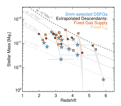
Aside from the simple comparison of volume densities between MORA DSFGs and quiescent galaxies at high-$z$, we can more closely consider the established stellar masses of MORA-selected galaxies, their potential for future star formation, and their likely descendant population. In other words, what stellar masses do we expect MORA-descendant galaxies to have after eventually ceasing their star formation? And at what redshift are those descendants fully formed? Figure 13 shows the extrapolated masses and redshifts for two hypothetical quiescent descendant populations from the MORA sample of DSFGs. The first assumes the lion’s share of the ISM mass (in the form of H₂) is converted into stars at the current (observed) SFR until that gas is fully depleted without replenishment. On average, the gas depletion time for the MORA sample is $\tau_{\rm depl}=110^{+30}_{-60}$ Myr. The second adopts an average starburst timescale of $\sim$100 Myr (in line with measurement of other DSFG samples, as well as the MORA sample herein, e.g. Bothwell et al., 2013) and presumes star formation will continue at the observed high rate for that fixed period of time before ceasing. The redshifts of the descendant population of quiescent systems is offset from the measured MORA redshifts by the measured or adopted gas depletion time. Note that there is no systematic offset of one population of hypothetical descendants from the other; half of the sample has higher masses and lower redshifts calculated with one method. Depending on the existing stellar reservoir, we find that anywhere between $\approx$ 20–100% of the eventual stellar mass in MORA descendants will form in the observed star forming episode. The final stellar masses of these systems is then $\sim$2$\times 10^{11}$  M_⊙, with the entire MORA 2 mm sample producing galaxies with stellar masses in excess of $>4\times 10^{10}$  M_⊙; this is well aligned with the measured mass limits and redshift regimes of high-$z$ quiescent galaxy surveys.

6.3 Is the emissivity spectral index steep, and/or does it evolve?

The dust emissivity spectral index, or $\beta$, governs the frequency dependence of the emissivity of dust grains per unit mass, such that $\kappa_{\nu}=\kappa_{0}(\nu/\nu_{0})^{\beta}$. The mass absorption coefficient, $\kappa_{\nu}$, traces the chemical and optical properties of dust grains. A lower value of $\beta$ observationally manifests in a shallower Rayleigh-Jeans fall off to the SED in the millimeter, while higher values result in steeper Rayleigh-Jeans fall offs.

Data on high-redshift galaxies – where the FIR/mm SED is spatially unresolved and poorly sampled – is of limited use in constraining the intrinsic dust emissivity spectral index, which relates to fundamental dust composition and likely varies on the scale of molecular clouds. For example, Arendt et al. (2019) measure an average value of $\beta=2.25$ for the central molecular zone (CMZ) in the Galactic plane of the Milky Way using new 2 mm GISMO observations; this is broadly in line with findings from Planck, which revealed $\beta\approx 1.6$ at high Galactic latitudes but increasingly steep values, $\beta=1.8-2.0$ toward the inner Galactic plane ($|b|\geq 10^{o}$ Planck Collaboration et al., 2014). Despite our inability to constrain the underlying physical quantity $\beta$, measurement of the slope of the Rayleigh-Jeans fall off, as captured by the galaxy-integrated $\beta$ calculated herein, is useful. Elucidating our view of the average galaxy-integrated $\beta$ is useful for relating galaxies’ dust SEDs to the (sub)millimeter surveys used to identify DSFGs in the first instance, simulating galaxies’ SEDs and SED fitting to high-$z$ unresolved sources.

Our measurement of $\langle\beta\rangle=2.2^{+0.5}_{-0.4}$ within this sample is consistent with the often assumed fixed value of $\beta\equiv 1.8$, though also suggestively a bit steeper (c.f. the prevailing theory based on ISM composition would suggest values of $\beta=1-2$; Draine, 2011). The analysis of SCUBA-2 selected sources sitting inside the MORA mosaic (in § 5.5) are similarly consistent with a range in $\beta$ that skew a bit higher than $\beta>1.8$, as shown in Figure 11. How do we interpret these relatively steep values of $\beta$ relative to shallower values in integrated SEDs of well constrained local Universe dust (Dunne & Eales, 2001; Clements et al., 2010)? While this could be suggestive of a higher proportion of large silicate grains in higher redshift dusty galaxies, it could also mark different underlying ISM geometries.

Theoretically, low values (e.g. $\beta\approx 1$) correspond to dust comprised of small amorphous carbons with a mix of underlying dust temperatures from warm to cold; this can be easily understood from the SED that would result from coadding several blackbodies of different temperatures yet similar masses: the net unresolved SED would have a shallower Rayleigh-Jeans tail than a dust distribution of any one temperature. Indeed, coadding spatially-distinct SEDs over the scale of an entire galaxy would always result in a shallowing of the Rayleigh-Jeans tail and not a steepening. One conjecture in the literature (e.g. Jin et al., 2019) is that the steepening of the Rayleigh-Jeans tail may be due to CMB heating of the SED at high redshifts, which would cause a greater reduction in the observed flux density at longer wavelengths relative to shorter wavelengths (da Cunha et al., 2013). However, CMB heating is likely only a significant effect for galaxies at $z\lower 2.15277pt\hbox{$\;\buildrel>\over{\sim}\;$}5$ at very low dust temperatures ($T<30\,$K) where the CMB temperature is non-negligible; furthermore, our SEDs do account for this CMB heating (however negligible), and our derived $\beta$ values still hold after accounting for this effect. While steeper values of $\beta$ can also indicate the presence of large crystalline silicate grains that reach overall lower temperatures (Draine & Lee, 1984; Agladze et al., 1996; Meny et al., 2007), the degeneracies between spatial distribution of the ISM, dust temperature, opacity and $\beta$, as well as the relative measurement uncertainties on our measurements from a dearth of data prevents any direct constraints on dust composition. Still it is an interesting puzzle that our galaxy-integrated $\beta$ seems to skew high relative to prevailing literature (see also Kato et al., 2018), that has, for lack of direct constraints, fixed the value to either $\beta=1.5$ (Paradis et al., 2009) or $\beta=1.8$ (Planck Collaboration et al., 2011) from measurements of the Milky Way’s ISM in both atomic and molecular states.

Our measurements of $\beta=2.2^{+0.5}_{-0.4}$, along with other recent direct measurements of $\beta$ in high-$z$ DSFGs (see da Cunha et al., 2021, who measure $\beta=1.9\pm 0.4$ for the ALESS sample via dedicated 2 mm follow-up observations), suggest that a higher $\beta\approx 2$ is more appropriate than $\beta=1.5$ or $\beta=1.8$ in instances where a DSFGs’ Rayleigh-Jeans tail is not directly constrained and a choice of $\beta$ is needed to model sources’ SEDs.

6.4 Potential Impact of Cosmic Variance on $z>3$ DSFG sample

Figure 14: Cosmic variance, $\sigma^{2}_{\rm v}$, as a function of survey solid angle for 2mm-detectable galaxies above $S_{\rm 2mm}>$0.3 mJy and a range of redshifts drawn from: the 108 deg² Shark lightcone (solid lines; Lagos et al., 2020) and the 7.7 deg² UniverseMachine lightcone (dot-dashed lines Popping et al., 2020). The gray shaded regions denote $\sigma_{\rm v}^{2}>0.15$ (and $>$0.20), a threshold representing significant (severe) cosmic variance. We show cosmic variance for sources above redshifts $z=4$ (purple lines), $z=4.5$ (green lines), $z=5$ (orange lines), and $z=5.5$ (red lines). Sources at higher redshifts are exceedingly rare ($\sim$1 deg^-2) in both Shark and UniverseMachine such that direct estimates of cosmic variance $\sigma_{v}^{2}$ cannot be reliably estimated. The size of the MORA survey is indicated with the vertical gray dashed line. We find that 2 mm sources are roughly a factor of $\sim$2$\times$ more rare in the UniverseMachine lightcone relative to Shark, and so the cosmic variance is appreciably higher. This work suggests a significant jump in survey area is needed – exceeding 0.2-0.3 deg² – to take an accurate census of DSFGs beyond $z>5.5$, while surveys of order a few tenths of a square degree are adequate at lower redshifts. It is likely that surveys exceeding 1 deg² will be needed to sample $z>6$ DSFGs well.

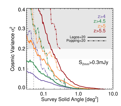
Though our MORA survey area is among the largest mosaics stitched together by ALMA to date, a chief concern of our analysis is that cosmic variance may impact our measurement of the ubiquity of DSFGs beyond $z>3$. In other words, our relatively small area — small in comparison to the relative rarity of DSFGs themselves — may oversample or undersample the average density of the Universe at any given epoch. Our parallel paper, Z21, tests the impact of cosmic variance using dust emission models applied to galaxies inside large volume simulations (see Z21, their section 4.4, as well as Popping et al., 2020). In those simulations, Z21 determines that the MORA survey volume is robust in the measurement of the number counts of 2 mm sources out to $z\sim 7$.

Here we extend the cosmic variance analysis of Z21 to analyze the cosmic variance specifically for the $z>4$ high-redshift tail of the 2 mm-observed population, and also incorporating predictions from the Shark semi-empirical model (Lagos et al., 2020). The definition of cosmic variance as given in Moster et al. (2011) is:

$$\sigma_{v}^{2}=\frac{\langle N^{2}\rangle-\langle N\rangle^{2}-\langle N\rangle}{\langle N\rangle^{2}},$$ (2)

where $N$ represents the number of galaxies detectable in a given survey solid angle above a redshift $z$. In other words, we generate Monte Carlo trial mock surveys with increasing area $\Omega$ within the Popping et al. (2020) and Lagos et al. (2020) lightcones and assess how many sources in these lightcones would be 2 mm detectable (at the rough sensitivity of the MORA survey) above a given redshift. At a fixed survey area, $\Omega$, we generate a distribution of $N$ that satisfy $S_{\rm 2mm}>0.3$ mJy and $z>4$ (or other higher redshift minima); from that distribution of $N$, we are able to easily compute $\langle N\rangle$ and $\langle N^{2}\rangle$ from which we calculate $\sigma_{v}^{2}$.

Our results are shown in Figure 14 where surveys with $\sigma_{\rm v}^{2}<0.15$ are less prone to the effects of cosmic variance. We find that, due to the relative rarity of dusty sources in both Shark and UniverseMachine, the MORA survey size ($\sim$0.05 deg²) is prone to cosmic variance above $z>4$ (according to UniverseMachine) and $z>5$ (according to Shark). The UniverseMachine generated lightcone has roughly a factor of $2-3\times$ fewer high SFR (SFR$\;\buildrel>\over{\sim}\;$100  M_⊙ yr^-1) galaxies than Shark at these redshifts and so the estimated cosmic variance is higher. Both models imply that significantly larger areas are needed to survey the $z>5.5$ Universe, of order 0.2-0.3 deg² or greater to suppress cosmic variance below $\sigma_{v}^{2}<0.15$. Given the dearth of $z>6$ DSFGs in both models, it is hard to characterize what survey area would be necessary to mitigate cosmic variance at those epochs, though naturally we may expect it to be $\;\buildrel>\over{\sim}\;$ 1 deg².

Note too that the uncertainties for the predicted model redshift distributions and number counts, shown in Figure 5, account for the same cosmic variance discussed here by sampling different regions of either lightcone over the 184 arcmin² MORA survey footprint. Those estimates account for the heterogeneous noise characteristics of the MORA survey, while the cosmic variance estimates in Figure 14 assume a uniform flux density threshold of $S_{\rm 2mm}>0.3$ mJy.

6.5 Potential Degeneracies in Interpretation

This paper has so far argued that 2 mm continuum observations can provide great clarity on the earliest epoch of dust-obscured galaxies at $z\lower 2.15277pt\hbox{$\;\buildrel>\over{\sim}\;$}4$, but how might our conclusions be impacted by astrophysical unknowns? The MORA survey represents an important step in constraining the obscured Universe in this early epoch, but further refinements will require data to break certain degeneracies, including unknowns about a possible evolving shape in the IRLF, galaxies’ evolving dust SEDs, and dust emissivities.

For example, there is substantial evidence to suggest that the faint-end slope of the UVLF evolves, such that it is much steeper at higher redshifts (Finkelstein, 2016). The physical interpretation of this is that there are far more low mass galaxies at early times, and with time the distribution of galaxies in the luminosity function is distributed across a larger dynamic range. Does the IRLF evolve similarly, differently, in the opposite sense, or not at all?

As presented in Figure 12, our data are consistent with a non-evolving faint-end slope of the IRLF, though the constraints do not rule out such an evolution. Being able to measure such an evolution will require more painstakingly deep observations (as can be provided by ALMA with deep 1–2 mm surveys at $<$1 mJy depth, like ASPECS, González-López et al. 2020) over significantly larger areas ($\;\buildrel>\over{\sim}\;$0.2 deg²). Furthermore, source redshifts – likely most efficiently obtained through large-area blind searches for millimeter spectral lines – will be paramount to this measurement. At present, no large field of view millimeter spectrometer exists with the needed sensitivity. Once in hand, the combination of a well-measured UVLF and IRLF, as well as the nature of their evolution, can directly inform models of early universe dust formation and attenuation.

The question of evolution in galaxies’ dust SEDs has come up frequently in recent literature (e.g. Ma et al., 2019; Liang et al., 2019) and may have significant impact on the results discussed herein and in Z21. For example, if $z>5$ galaxies contain, on average, substantially hotter dust than lower redshift DSFGs as such works suggest (with correspondingly lower dust mass per fixed L_IR), then it is likely that 2 mm dust continuum maps could miss upwards of half of all DSFGs at early epochs. In other words, if the average dust SED is hotter at high redshifts, then those SEDs peak at shorter rest-frame wavelengths and are likely to have lower flux densities on the Rayleigh-Jeans tail (2 mm observed) than colder DSFGs. This would lead to a smaller fraction of DSFGs being detected at 2 mm, and it would be logical to conclude that our results have under-estimated the total volume density of early Universe DSFGs (a point raised as a hypothetical in Casey et al., 2018b). If that is the case, then some tension may exist between the inferred volume density of all DSFGs and the measured volume density of lower redshift quiescent galaxies (as discussed in § 6.2). Nevertheless, with exception of very luminous lensed systems (e.g. Reuter et al., 2020) the spectral energy distributions of DSFGs at $z>4$ are not well constrained as an aggregate population. Measuring them will provide invaluable insight into both ISM physics in the first few Gyr as well as further constraints on the volume density measurements of the population themselves.

Variation in the dust emissivity index may also impact our volume density constraints in a similar fashion to variation in the aggregate dust temperatures of early DSFGs. With a steeper $\beta$, flux densities on the Rayleigh-Jeans tail drop; for example, the 2 mm flux density of a galaxy at $z=4$ would be three times lower for a very steep $\beta=3.5$ than for a shallower value $\beta=1.5$, presuming a fixed value of L_IR and $\lambda_{\rm peak}$. As discussed in § 6.3, our sample does show moderate evidence for steeper emissivity spectral indices across the sample. If DSFGs on a whole were to exhibit steeper Rayleigh-Jeans tails it may imply that our volume density measurements here, and in Z21, are underestimated.

Lastly, it is crucial to point out that many MORA source redshifts are not yet well constrained. Given our small sample size, even one catastrophically mis-identified redshift would shift our integrated SFRD results by $\sim$10%, and thus has potential to alter our perception of the IRLF’s evolution beyond $z>3$.

6.6 Future Surveys of $z\lower 2.15277pt\hbox{$\;\buildrel>\over{\sim}\;$}4$ Obscured Sources

Future 2 mm surveys of large areas of sky will be crucial to overcome limitations of small sample sizes and cosmic variance, particularly in pursuit of rare, dusty starbursts at $z>4$. In particular, testing the divergent redshift distribution predictions for bright DSFGs ($S_{\rm 2mm}>1\,$mJy; see Figure 6) in the simulations will be an essential next step. While the Shark and UniverseMachine simulations predict that the brightest 2 mm sources have a relatively low median redshift ($\langle z\rangle\sim 2.5$), the SIDES, Casey et. al. and Zavala et. al. models suggest a higher average redshift ($\langle z\rangle\lower 2.15277pt\hbox{$\;\buildrel>\over{\sim}\;$}3.5$). This difference originates with the fundamental problem of how massive, bright galaxies assemble en-masse so quickly after the Big Bang. Sampling these bright sources in statistically large samples well will truly require a different scale of millimeter continuum survey, of order $\;\buildrel>\over{\sim}\;$5 deg², as such bright high-$z$ systems are predicted to be extremely rare in the models (e.g. SHARK predicts five $z>4$ sources per square degree above 1 mJy at 2 mm, and only one such source above $z>5$ per square degree). While large-field searches of Herschel SPIRE imaging for 500$\mu$m-peaking “red” sources has been fruitful (Ivison et al., 2016; Duivenvoorden et al., 2018; Yan et al., 2020), the population is quite rare ($\sim$10^-7 Mpc^-3) relative to the MORA-detected DSFGs presented herein, due to the relative shallow sensitivity of Herschel at high redshifts. Instruments like GISMO, which has pioneered much of the 2 mm blank-field mapping work to-date, and TolTEC, which in the future has the potential to expand 2 mm sky coverage by orders of magnitude, will play essential roles in pushing this frontier. Similarly, the South Pole Telescope survey has already demonstrated the effectiveness of $>$1 mm surveys in recovering an intrinsically high-$z$ population (see Vieira et al., 2013; Reuter et al., 2020), and the next generation SPT survey (‘SPT3G’) will push the depth such that unlensed sources will be detected at high significance.

One complementary observing strategy to large surveys would be dedicated 2 mm–3 mm continuum follow-up of DSFGs already identified at shorter wavelengths, allowing a more efficient redshift selection of the highest-$z$ sources using millimeter colors. Every source in the MORA Survey (save one that we attribute to a false noise peak) is detected above 3.5 $\sigma$ significance at 850$\mu$m, and many at other (sub)mm wavelengths from existing single dish surveys. As Figure 11 shows, the MORA sources with lower $S_{\rm 870}/S_{\rm 2000}$ ratios sit at the highest redshifts as would be expected for sources whose 850$\mu$m emission is closer to the peak of dust emission. Though strategic 2 mm or 3 mm follow-up of 850$\mu$m or 1 mm-selected sources is more biased than the blank field survey strategy, it is far more observationally efficient for samples that have already been identified, requiring only a few minutes of on-source time with ALMA. It is an effective, and observationally cheap filter through which needles ($z>4$ DSFGs) can be spotted in the haystack (dominated by $1<z<3$ DSFGs), complementing 2 mm blank field surveys like MORA.

Lastly, extentions of MORA stand to make significant progress; over the next year, MORA is approved for observations to expand coverage over 0.2 deg² (within the COSMOS-Webb survey footprinto) to the same depth of our current mosaics. These data will likely lead to the discovery of $\sim$20 DSFGs at $z>4$ and enable more detailed studies of DSFG clustering.

7 Conclusions

We have presented the Mapping Obscuration to Reionization with ALMA (MORA) Survey, the first 2 mm extragalactic blank field map with ALMA covering 184 arcmin². Our accompanying paper, Zavala et al. (2021), presents the MORA Survey number counts and number count-constrained obscured star-formation rate density measurement out to $z\sim 7$, while this paper focuses on what is known about the individual galaxies that have been detected. We detect thirteen sources above $>$5$\sigma$ significance, one of which may have significant contribution from radio synchrotron emission and another we believe to be a false-positive noise peak, leaving a total of eleven robust detections dominated by thermal dust emission. The redshifts of the sources span $z=2.2-5.9$ with a median redshift of $\langle z\rangle=3.6^{+0.4}_{-0.3}$. Sources span IR luminosities $10^{12}-{\rm few}\times 10^{13}$  L_⊙, ISM masses ${\rm few}\times 10^{10}-{\rm few}\times 10^{11}$  M_⊙, and sit both above and embedded within the galaxy SFR-stellar mass relation.

Our results paint a plausible picture of the build-up of dust-obscured galaxies at the earliest epochs ($z>4$): overall, DSFGs at this epoch are rare and contribute a sizable, though non-dominant, fraction towards cosmic star formation. These DSFGs are the most likely progenitors of the Universe’s first massive, quiescent galaxies. Our primary conclusions are as follows:

1. ALMA Band 4 (2 mm) is an effective selection wavelength for high-$z$ DSFGs; here we find 77$\pm$11 % of our 2 mm-selected sample lies above $z>3$ and 38$\pm$12 % above $z>4$. This contrasts with more traditional methods of DSFG selection at 850$\mu$m or 1 mm, whose proportion of sources at these redshifts is much smaller (e.g. 6% of 850$\mu$m-selected sources sit at $z>4$; Dudzevičiūtė et al., 2020).

2. “OIR-dark” sources (i.e. sources lacking counterparts in very deep optical and near-infrared data, $<$1.6 $\mu$m) make up a sizable fraction of 2 mm selected sources (4/11$\sim$36%). Our accompanying paper, Manning et. al. in prep further explores their physical characteristics.

3. Several semi-empirical and empirical models from the literature accurately reproduce the redshift distribution and volume density of 2 mm-detected galaxies. However, several details are not yet resolved by data, namely the epoch when the first DSFGs turn on, and how common such systems are at the highest redshifts, $z\lower 2.15277pt\hbox{$\;\buildrel>\over{\sim}\;$}5.5$. Different cosmological models infer that MORA may be impacted by cosmic variance above $z>5$, with the results highly dependent on dust radiation prescriptions in early Universe galaxies. Either way, larger area 2 mm continuum surveys will be essential to gather sufficient statistics to constrain the volume density of DSFGs at the highest-redshift regimes.

4. Dusty galaxies with star-formation rates in excess of 300  M_⊙ yr^-1 contribute $\sim$30% to SFRD between $3<z<6$. Furthermore, at these epochs, the IRLF is dominated by these sources, with little contribution from galaxies with lower levels of obscured star formation ($\;\buildrel<\over{\sim}\;$ 100  M_⊙ yr^-1). This implies that the vast majority of cosmic dust lives in such ultraluminous galaxies at these epochs, with relatively little to no dust impacting the bolometric output of less luminous, less massive systems.

5. DSFGs at $z>3$, like those detected in the MORA Survey, are often claimed to be the progenitors of the Universe’s earliest quiescent systems; we find that the number density of quiescent galaxies from the literature agrees well with the measured volume density of DSFGs measured at $z>3$ ($\sim$10^-5 Mpc^-3). Furthermore, the extrapolated characteristics of MORA DSFGs’ descendants are also well aligned with detected quiescent populations, all well established with stellar masses $>$10¹¹  M_⊙ above $z>2$.

6. Our MORA data hints at a possible higher value for the galaxy-integrated dust emissivity index, $\beta$, than is often assumed in the literature: the sample has a measured $\langle\beta\rangle=2.2^{+0.5}_{-0.4}$ vs $\beta=1.8$. We recommend future works modeling SEDs of high-$z$ DSFGs adopt a value of $\beta\approx 2$ as needed in lieu of direct constraints.

The final frontier of this work would lead to the detection of the Universe’s first dusty galaxies, the home of the Universe’s first substantial dust reservoirs. Do such systems exist beyond $z>7$? $z>8$? While MORA has taken a tantalizing first step in completing the census of high-$z$ DSFGs, we know higher redshift DSFGs (specifically, three with ${\rm SFR}\lower 2.15277pt\hbox{$\;\buildrel>\over{\sim}\;$}100$  M_⊙ yr^-1) do exist than are found in this work (e.g. Cooray et al., 2014; Zavala et al., 2018b; Strandet et al., 2017; Marrone et al., 2018). Yet, their rarity – itself not yet well constrained – implies that finding more requires large area millimeter surveys sufficiently sensitive to detect unlensed galaxies, similar conceptually to the all-sky searches for the highest redshift quasars found by, e.g., the Sloan Digital Sky Survey (Fan et al., 2001, 2003). And though rare, the earliest dusty starbursts yet to be found serve as unique laboratories for our understanding of the assembly of the first galaxies and, fundamentally, the formation of dust, on which much of what we know about the modern day Universe relies.

Table 3: Photometry of the $>$5$\sigma$ 2 mm Sample.

Name	Position	SNR2mm	S${}_{\rm 2\,mm}$	$H$-band	S3.6	S24	S100	S160	S250	S350	S450	S500	S850	S${}_{\rm 1.2\,mm}$	S3GHz
	($\alpha_{\rm J2000}$, $\delta_{\rm J2000}$)		[$\mu$Jy]	[AB]	[nJy]	[$\mu$Jy]	[mJy]	[mJy]	[mJy]	[mJy]	[mJy]	[mJy]	[mJy]	[mJy]	[$\mu$Jy]
MORA-0	10:00:15.617 $+$02:15:49.00	7.90	818$\pm$103	—	1714$\pm$40	[21$\pm$27]	[$-$1.5$\pm$1.7]	[0.6$\pm$3.7]	[8.9$\pm$5.8]	[18.7$\pm$6.3]	[10.7$\pm$5.8]	[20.3$\pm$6.8]	13.56$\pm$0.12†	4.13$\pm$0.18	19.5$\pm$2.6
MORA-1	10:00:19.740 $+$02:32:03.80	7.74	703$\pm$91	22.68$\pm$0.02	6958$\pm$94	189$\pm$13	[0.0$\pm$1.7]	31.4$\pm$3.7	37.6$\pm$5.8	48.4$\pm$6.3	29.2$\pm$5.2	35.7$\pm$6.8	8.67$\pm$0.06†	2.67$\pm$0.09	74.8$\pm$0.9∗
MORA-2	10:00:10.146 $+$02:13:35.00	7.58	529$\pm$70	24.24$\pm$0.04	5223$\pm$100	[18$\pm$25]	[3.9$\pm$1.7]	13.1$\pm$3.8	15.4$\pm$5.8	31.3$\pm$6.3	[17.2$\pm$9.4]	27.7$\pm$6.8	8.82$\pm$0.71	2.66$\pm$0.05	30.1$\pm$2.9
MORA-3	10:00:08.037 $+$02:26:12.20	7.25	1220$\pm$168	…	…	…	[0.3$\pm$1.7]	[1.0$\pm$3.7]	[16.8$\pm$5.8]	30.8$\pm$6.3	23.5$\pm$4.8	29.1$\pm$6.8	16.75$\pm$0.15†	4.62$\pm$0.11	15.0$\pm$2.4
MORA-4	10:00:26.359 $+$02:15:28.00	6.68	557$\pm$83	—	87$\pm$29	[10$\pm$18]	[0.5$\pm$1.5]	[-0.6$\pm$2.8]	[2.9$\pm$5.8]	[2.9$\pm$6.3]	[2.3$\pm$5.8]	[4.9$\pm$6.8]	5.908$\pm$0.052†	2.05$\pm$0.11	[10.6$\pm$4.1]
MORA-5	10:00:24.157 $+$02:20:05.40	6.63	584$\pm$88	—	406$\pm$24	[-8$\pm$26]	[-0.2$\pm$1.7]	[-0.1$\pm$3.7]	[3.8$\pm$5.8]	[7.3$\pm$6.3]	[10.7$\pm$4.1]	[7.1$\pm$6.8]	6.80$\pm$0.53	2.30$\pm$0.10	[10.1$\pm$3.4]
MORA-6	10:00:28.723 $+$02:32:03.40	6.37	615$\pm$97	23.75$\pm$0.03	4332$\pm$30	198$\pm$13	[-0.4$\pm$1.7]	19.3$\pm$3.3	34.7$\pm$5.8	35.0$\pm$6.3	40.6$\pm$5.2	24.8$\pm$6.8	12.57$\pm$0.15†	3.13$\pm$0.10	45.5$\pm$0.8∗
MORA-7	10:00:11.574 $+$02:15:05.20	6.29	378$\pm$60	23.52$\pm$0.02	11956$\pm$80	175$\pm$16	[0.6$\pm$1.8]	[-0.3$\pm$3.8]	[16.1$\pm$5.8]	[17.0$\pm$6.3]	20.7$\pm$6.6	[9.5$\pm$6.8]	5.31$\pm$0.16†	1.51$\pm$0.13	12.2$\pm$2.3
MORA-8	10:00:25.292 $+$02:18:46.20	5.75	489$\pm$85	23.21$\pm$0.02	11156$\pm$79	204$\pm$29	[-1.7$\pm$1.9]	[0.6$\pm$3.8]	[16.2$\pm$5.8]	24.7$\pm$6.3	15.2$\pm$4.3	26.8$\pm$6.8	7.12$\pm$0.54	…	34.7$\pm$2.9
MORA-9	10:00:17.298 $+$02:27:15.80	5.55	379$\pm$68	26.75$\pm$0.30	469$\pm$33	[1$\pm$13]	[-0.5$\pm$1.7]	[-0.3$\pm$3.7]	[0.0$\pm$5.8]	[0.0$\pm$6.3]	[1.1$\pm$4.1]	[0.0$\pm$6.8]	2.59$\pm$0.37†	…	[4.3$\pm$2.4]
MORA-10	10:00:16.578 $+$02:26:38.00	5.21	405$\pm$78	22.77$\pm$0.01	10766$\pm$66	890$\pm$17	5.8$\pm$1.7	18.9$\pm$4.0	[15.6$\pm$5.8]	[17.4$\pm$6.3]	20.4$\pm$4.1	[8.5$\pm$6.8]	6.07$\pm$0.07†	…	3212.0$\pm$1.6∗
MORA-11	10:00:12.922 $+$02:12:11.40	5.16	356$\pm$69	22.64$\pm$0.01	13322$\pm$199	[22$\pm$44]	[0.5$\pm$1.6]	[0.4$\pm$3.1]	35.7$\pm$15.8	40.0$\pm$20.3	[7.6$\pm$14.4]	41.9$\pm$25.9	5.10$\pm$0.78	1.49$\pm$0.07	12.1$\pm$2.4
MORA-12	10:00:04.713 $+$02:29:55.20	5.03	950$\pm$190	—	[1$\pm$30]	[1$\pm$12]	[0.7$\pm$1.7]	[0.4$\pm$3.7]	[13.8$\pm$5.8]	[14.2$\pm$6.3]	[1.2$\pm$4.8]	[5.7$\pm$6.8]	[0.22$\pm$0.69]	…	[1.0$\pm$2.3]

Table Notes. Photometry enclosed in brackets represent $<$3$\sigma$ detections. Ellipses (…) indicate an absence of data while long dashes (—) represent a non-detection in the COSMOS2020 catalog. Note that MORA-3 has highly confused Spitzer imaging, blending MORA-3 with two lower redshift foreground sources within the Spitzer beam at both 3.6$\mu$m and 24$\mu$m. A dagger ($\dagger$) indicates that the flux density in the 850$\mu$m column has been replaced by improved 870$\mu$m photometry from ALMA rather than SCUBA-2. An asterisk (^∗) indicates that the 3 GHz flux density comes from the deeper COSMOS-XS maps of van der Vlugt et al. (2021) and Algera et al. (2020) rather than the shallower/wider coverage of Smolčić et al. (2017). Note that some of the sample have ALMA band 6 data from archival datasets (recorded here at 1.2 mm).

Table 4: Positions and Multiwavelength Counterparts for the Marginal $4<\sigma<5$ 2 mm sample

Name	Position	SNR2mm	S${}_{\rm 2\,mm}$	$H$-band	S850	S3GHz
	($\alpha_{\rm J2000}$, $\delta_{\rm J2000}$)		[$\mu$Jy]	[AB]	[mJy]	[$\mu$Jy]
MORA-P03-0	10:00:42.629 $+$02:14:39.00	4.68	615$\pm$131	…	…	…
MORA-P03-1	10:00:42.843 $+$02:14:59.80	4.51	493$\pm$109	…	…	…
MORA-P03-2	10:00:43.643 $+$02:22:05.20	4.37	308$\pm$70	…	…	…
MORA-P03-3	10:00:42.415 $+$02:27:18.60	4.28	703$\pm$164	…	…	…
MORA-P03-4	10:00:46.019 $+$02:28:29.20	4.24	506$\pm$119	…	…	…
MORA-P03-5	10:00:42.629 $+$02:18:29.20	4.19	551$\pm$131	…	…	…
MORA-P03-6	10:00:42.362 $+$02:26:56.60	4.07	711$\pm$174	…	…	…
MORA-P03-7	10:00:45.685 $+$02:24:26.40	4.07	378$\pm$93	…	…	…
MORA-P03-8	10:00:45.818 $+$02:13:06.20	4.07	416$\pm$102	…	…	…
MORA-P03-9	10:00:44.511 $+$02:15:49.20	4.04	256$\pm$63	…	…	…
MORA-P03-10	10:00:42.936 $+$02:11:51.00	4.01	408$\pm$102	…	…	…
MORA-13	10:00:24.398 $+$02:21:45.00	4.78	419$\pm$88	…	…	…
MORA-14	10:00:26.119 $+$02:19:07.80	4.74	397$\pm$84	…	…	…
MORA-15	10:00:25.118 $+$02:15:37.20	4.68	398$\pm$85	…	…	…
MORA-16	10:00:25.505 $+$02:20:30.20	4.68	397$\pm$85	…	…	…
MORA-17	10:00:27.761 $+$02:24:43.40	4.61	406$\pm$88	26.74$\pm$0.24	…	…
MORA-18	10:00:23.103 $+$02:12:27.40	4.59	401$\pm$88	26.19$\pm$0.14	…	…
MORA-19	10:00:12.000 $+$02:23:09.80	4.58	283$\pm$62	25.00$\pm$0.16	4.00$\pm$0.57	259.0$\pm$2.9
MORA-20	10:00:24.572 $+$02:32:03.00	4.58	404$\pm$88	…	…	30.3$\pm$3.9∗
MORA-21	10:00:06.543 $+$02:21:31.60	4.54	414$\pm$91	26.81$\pm$0.50	…	…
MORA-22	10:00:12.960 $+$02:32:31.00	4.54	304$\pm$67	…	…	…
MORA-23	10:00:12.575 $+$02:14:44.20	4.52	298$\pm$66	21.30$\pm$0.01	7.19$\pm$0.64	…
MORA-24	10:00:07.837 $+$02:21:05.20	4.52	656$\pm$145	24.88$\pm$0.08	…	…
MORA-25	10:00:23.970 $+$02:17:49.80	4.52	398$\pm$88	18.94$\pm$0.01	10.48$\pm$0.55	96.8$\pm$2.8
MORA-26	10:00:22.716 $+$02:25:31.80	4.51	397$\pm$88	…	…	…
MORA-27	10:00:22.636 $+$02:23:04.20	4.46	392$\pm$88	…	…	…
MORA-28	10:00:24.945 $+$02:24:05.60	4.46	385$\pm$86	…	…	…
MORA-29	10:00:23.650 $+$02:21:55.40	4.34	389$\pm$89	23.21$\pm$0.02	7.87$\pm$0.55	256$\pm$2.4
MORA-30	10:00:14.563 $+$02:16:45.00	4.34	422$\pm$97	…	…	…
MORA-31	10:00:24.038 $+$02:29:48.20	4.32	383$\pm$89	26.14$\pm$0.16	6.12$\pm$0.62	…
MORA-32	10:00:20.434 $+$02:32:57.80	4.29	397$\pm$93	…	…	…
MORA-33	10:00:05.274 $+$02:23:58.40	4.29	529$\pm$123	…	…	…
MORA-34	10:00:27.748 $+$02:26:45.40	4.29	377$\pm$88	…	…	…
MORA-35	10:00:20.768 $+$02:13:16.20	4.28	382$\pm$89	…	…	…
MORA-36	10:00:27.280 $+$02:20:16.80	4.28	364$\pm$85	…	…	…
MORA-37	10:00:15.870 $+$02:24:46.00	4.27	424$\pm$99	…	5.38$\pm$0.58	…
MORA-38	10:00:18.219 $+$02:18:51.60	4.27	311$\pm$73	…	…	…
MORA-39	10:00:25.438 $+$02:15:58.80	4.27	360$\pm$84	…	…	…
MORA-40	10:00:05.863 $+$02:16:08.40	4.26	416$\pm$98	…	…	6.4$\pm$1.0∗
MORA-41	10:00:05.875 $+$02:26:16.20	4.25	414$\pm$97	…	…	…
MORA-42	10:00:22.783 $+$02:16:07.80	4.25	373$\pm$88	…	…	…
MORA-43	10:00:30.736 $+$02:15:47.00	4.25	1140$\pm$268	…	…	…
MORA-44	10:00:27.560 $+$02:21:58.20	4.25	368$\pm$87	…	…	…
MORA-45	10:00:15.603 $+$02:25:50.40	4.24	458$\pm$108	…	…	…
MORA-46	10:00:20.434 $+$02:28:03.00	4.23	389$\pm$92	…	…	…
MORA-47	10:00:15.964 $+$02:20:27.80	4.22	403$\pm$96	…	…	…
MORA-48	10:00:22.743 $+$02:32:41.00	4.21	373$\pm$89	…	…	…
MORA-49	10:00:30.097 $+$02:31:21.40	4.20	646$\pm$154	…	…	…
MORA-50	10:00:05.394 $+$02:29:44.20	4.20	487$\pm$116	…	…	…
MORA-51	10:00:25.333 $+$02:33:33.20	4.19	369$\pm$88	…	…	…
MORA-52	10:00:04.420 $+$02:28:00.80	4.19	1090$\pm$261	…	…	…
MORA-53	10:00:27.321 $+$02:31:40.60	4.19	358$\pm$86	…	5.95$\pm$0.68	…
MORA-54	10:00:16.751 $+$02:23:59.40	4.18	313$\pm$75	…	…	…
MORA-55	10:00:10.679 $+$02:21:41.60	4.17	258$\pm$62	…	…	…
MORA-56	10:00:28.108 $+$02:27:10.40	4.15	377$\pm$91	…	…	…
MORA-57	10:00:07.184 $+$02:14:58.20	4.14	427$\pm$103	23.69$\pm$0.03	…	…
MORA-58	10:00:06.823 $+$02:21:18.60	4.13	389$\pm$94	…	…	…
MORA-59	10:00:29.109 $+$02:29:10.80	4.13	427$\pm$103	…	…	…
MORA-60	10:00:05.637 $+$02:11:56.40	4.12	434$\pm$105	…	…	…
MORA-61	10:00:20.114 $+$02:18:01.40	4.12	375$\pm$91	…	…	…
MORA-62	10:00:30.684 $+$02:31:26.00	4.12	1030$\pm$251	23.21$\pm$0.01	…	…
MORA-63	10:00:27.614 $+$02:22:32.40	4.11	358$\pm$87	…	…	…
MORA-64	10:00:23.170 $+$02:28:51.40	4.11	364$\pm$89	…	…	…
MORA-65	10:00:13.762 $+$02:14:00.60	4.10	320$\pm$78	…	2.51$\pm$0.66	…
MORA-66	10:00:28.214 $+$02:19:53.20	4.09	380$\pm$93	…	3.10$\pm$0.53	…
MORA-67	10:00:28.923 $+$02:32:18.60	4.09	407$\pm$99	23.38$\pm$0.02	…	…
MORA-68	10:00:16.978 $+$02:28:13.00	4.09	290$\pm$71	…	…	…
MORA-69	10:00:25.332 $+$02:29:31.00	4.09	352$\pm$86	…	…	…
MORA-70	10:00:27.867 $+$02:19:51.80	4.08	366$\pm$90	…	3.10$\pm$0.53	…
MORA-71	10:00:28.175 $+$02:31:48.20	4.08	372$\pm$91	…	…	…
MORA-72	10:00:07.396 $+$02:23:44.60	4.08	460$\pm$113	…	…	…
MORA-73	10:00:12.934 $+$02:23:45.60	4.08	275$\pm$68	…	2.64$\pm$0.57	93.7$\pm$2.6
MORA-74	10:00:14.002 $+$02:23:33.40	4.08	336$\pm$82	…	…	…
MORA-75	10:00:06.104 $+$02:10:50.40	4.07	754$\pm$185	…	…	…
MORA-76	10:00:28.963 $+$02:30:13.60	4.07	408$\pm$100	…	…	…
MORA-77	10:00:05.410 $+$02:12:16.40	4.06	470$\pm$116	19.15$\pm$0.01	…	112.0$\pm$2.8
MORA-78	10:00:22.997 $+$02:28:09.40	4.06	359$\pm$88	…	…	…
MORA-79	10:00:09.370 $+$02:32:14.40	4.06	443$\pm$109	…	…	…
MORA-80	10:00:04.500 $+$02:28:58.60	4.06	963$\pm$237	…	…	25.7$\pm$3.3∗
MORA-81	10:00:26.492 $+$02:15:27.00	4.05	338$\pm$83	…	5.90$\pm$0.60	…
MORA-82	10:00:23.170 $+$02:17:38.60	4.05	357$\pm$88	…	…	…
MORA-83	10:00:22.410 $+$02:30:26.20	4.04	354$\pm$88	22.72$\pm$0.01	3.88$\pm$0.64	42.0$\pm$3.5
MORA-84	10:00:08.983 $+$02:32:08.00	4.04	617$\pm$152	…	…	…
MORA-85	10:00:21.902 $+$02:22:46.00	4.04	355$\pm$88	…	…	…
MORA-86	10:00:05.982 $+$02:25:12.40	4.04	384$\pm$95	…	…	…
MORA-87	10:00:07.368 $+$02:33:58.00	4.03	655$\pm$162	26.73$\pm$0.48	…	…
MORA-88	10:00:30.122 $+$02:20:38.60	4.03	637$\pm$158	…	…	57.1$\pm$0.9∗
MORA-89	10:00:29.629 $+$02:24:10.20	4.03	490$\pm$122	…	…	…
MORA-90	10:00:20.341 $+$02:16:49.60	4.03	366$\pm$91	…	…	…
MORA-91	10:00:08.129 $+$02:33:01.60	4.03	728$\pm$181	…	…	…
MORA-92	10:00:29.309 $+$02:25:54.20	4.02	438$\pm$109	…	…	…
MORA-93	10:00:26.773 $+$02:20:44.00	4.02	336$\pm$84	…	…	…
MORA-94	10:00:07.571 $+$02:16:31.40	4.01	492$\pm$122	…	…	…
MORA-95	10:00:25.745 $+$02:18:23.00	4.01	338$\pm$84	…	…	…
MORA-96	10:00:14.482 $+$02:28:48.40	4.01	385$\pm$96	20.81$\pm$0.01	…	…
MORA-97	10:00:06.729 $+$02:25:36.00	4.01	373$\pm$93	…	…	…
MORA-98	10:00:09.412 $+$02:22:02.20	4.00	419$\pm$105	…	…	…
MORA-99	10:00:19.660 $+$02:31:04.60	4.00	360$\pm$90	23.17$\pm$0.02	…	…

Table Notes. Marginal 2 mm sources and their multiwavelength counterparts, identified in the COSMOS2020 photometric catalog within 1^′′ of the 2 mm position (with $H$-band magnitude from UltraVISTA; Weaver et. al. submitted), at 850$\mu$m with SCUBA-2 within 8^′′ of the 2 mm position (Simpson et al., 2019), or at 3 GHz within 1^′′ of the 2 mm position (Smolčić et al., 2017). Sources marked with asterisks (^∗) have 3 GHz flux density measurements from the deeper COSMOS-XS survey (van der Vlugt et al., 2021; Algera et al., 2020).

References

- Agladze et al. (1996) Agladze, N., Sievers, A., Jones, S., Burlitch, J., & Beckwith, S. 1996, ApJ, 462, 1026, doi: 10.1086/177217
- Algera et al. (2020) Algera, H. S. B., van der Vlugt, D., Hodge, J. A., et al. 2020, ApJ, 903, 139, doi: 10.3847/1538-4357/abb77a
- Aravena et al. (2016) Aravena, M., Decarli, R., Walter, F., et al. 2016, ArXiv e-prints. https://arxiv.org/abs/1607.06772
- Aravena et al. (2020) Aravena, M., Boogaard, L., Gónzalez-López, J., et al. 2020, ApJ, 901, 79, doi: 10.3847/1538-4357/ab99a2
- Arendt et al. (2019) Arendt, R. G., Staguhn, J., Dwek, E., et al. 2019, ApJ, 885, 71, doi: 10.3847/1538-4357/ab451c
- Aretxaga et al. (2011) Aretxaga, I., Wilson, G., Aguilar, E., et al. 2011, MNRAS, 415, 3831, doi: 10.1111/j.1365-2966.2011.18989.x
- Arnouts et al. (2002) Arnouts, S., Moscardini, L., Vanzella, E., et al. 2002, MNRAS, 329, 355, doi: 10.1046/j.1365-8711.2002.04988.x
- Ashby et al. (2015) Ashby, M., Willner, S., Fazio, G., et al. 2015, ApJS, 218, 33, doi: 10.1088/0067-0049/218/2/33
- Bakx et al. (2018) Bakx, T. J., Eales, S., Negrello, M., et al. 2018, MNRAS, 473, 1751, doi: 10.1093/mnras/stx2267
- Battisti et al. (2019) Battisti, A., da Cunha, E., Grasha, K., et al. 2019, ApJ, 882, 61, doi: 10.3847/1538-4357/ab345d
- Behroozi et al. (2018) Behroozi, P., Wechsler, R., Hearin, A., & Conroy, C. 2018, ArXiv e-prints. https://arxiv.org/abs/1806.07893
- Bertin & Arnouts (1996) Bertin, E., & Arnouts, S. 1996, A&AS, 117, 393
- Bertoldi et al. (2007) Bertoldi, F., Carilli, C., Aravena, M., et al. 2007, ApJS, 172, 132, doi: 10.1086/520511
- Béthermin et al. (2012) Béthermin, M., Le Floc’h, E., Ilbert, O., et al. 2012, A&A, 542, A58, doi: 10.1051/0004-6361/201118698
- Bethermin et al. (2017) Bethermin, M., Wu, H.-Y., Lagache, G., et al. 2017, ArXiv e-prints. https://arxiv.org/abs/1703.08795
- Biggs & Ivison (2008) Biggs, A., & Ivison, R. 2008, MNRAS, 385, 893, doi: 10.1111/j.1365-2966.2008.12869.x
- Blain et al. (2002) Blain, A., Smail, I., Ivison, R., Kneib, J., & Frayer, D. 2002, Phys. Rep., 369, 111, doi: 10.1016/S0370-1573(02)00134-5
- Bothwell et al. (2013) Bothwell, M., Aguirre, J., Chapman, S., et al. 2013, ApJ, 779, 67, doi: 10.1088/0004-637X/779/1/67
- Bouwens et al. (2020) Bouwens, R., González-López, J., Aravena, M., et al. 2020, ApJ, 902, 112, doi: 10.3847/1538-4357/abb830
- Brammer et al. (2008) Brammer, G., van Dokkum, P., & Coppi, P. 2008, ApJ, 686, 1503
- Brisbin et al. (2017) Brisbin, D., Miettinen, O., Aravena, M., et al. 2017, ArXiv e-prints. https://arxiv.org/abs/1708.05748
- Bruzual & Charlot (2003) Bruzual, G., & Charlot, S. 2003, MNRAS, 344, 1000, doi: 10.1046/j.1365-8711.2003.06897.x
- Capak et al. (2007) Capak, P., Aussel, H., Ajiki, M., et al. 2007, ApJS, 172, 99, doi: 10.1086/519081
- Capak et al. (2010) Capak, P. L., Scoville, N., Sanders, D., et al. 2010, in American Astronomical Society Meeting Abstracts, Vol. 215, American Astronomical Society Meeting Abstracts #215, 410.05
- Caputi et al. (2017) Caputi, K., Deshmukh, S., Ashby, M., et al. 2017, ApJ, 849, 45, doi: 10.3847/1538-4357/aa901e
- Caputi et al. (2021) Caputi, K., Caminha, G., Fujimoto, S., et al. 2021, ApJ, 908, 146, doi: 10.3847/1538-4357/abd4d0
- Casey (2016) Casey, C. 2016, ApJ, 824, 36. https://arxiv.org/abs/1603.04437
- Casey et al. (2018a) Casey, C., Hodge, J., Zavala, J., et al. 2018a, ApJ, 862, 78, doi: 10.3847/1538-4357/aacd11
- Casey et al. (2014) Casey, C., Narayanan, D., & Cooray, A. 2014, Phys. Rep., 541, 45, doi: 10.1016/j.physrep.2014.02.009
- Casey et al. (2015) Casey, C., Cooray, A., Capak, P., et al. 2015, ApJ, 808, L33, doi: 10.1088/2041-8205/808/2/L33
- Casey et al. (2017) Casey, C., Cooray, A., Killi, M., et al. 2017, ApJ, 840, 101, doi: 10.3847/1538-4357/aa6cb1
- Casey et al. (2018b) Casey, C., Zavala, J., Spilker, J., et al. 2018b, ApJ, 862, 77, doi: 10.3847/1538-4357/aac82d
- Casey (2012) Casey, C. M. 2012, MNRAS, 425, 3094, doi: 10.1111/j.1365-2966.2012.21455.x
- Casey (2020) —. 2020, ApJ, 900, 68, doi: 10.3847/1538-4357/aba528
- Casey et al. (2013) Casey, C. M., Chen, C.-C., Cowie, L. L., et al. 2013, MNRAS, 436, 1919, doi: 10.1093/mnras/stt1673
- Casey et al. (2019) Casey, C. M., Zavala, J. A., Aravena, M., et al. 2019, ApJ, 887, 55, doi: 10.3847/1538-4357/ab52ff
- Chapman et al. (2005) Chapman, S., Blain, A., Smail, I., & Ivison, R. 2005, ApJ, 622, 772, doi: 10.1086/428082
- Chapman et al. (2003) Chapman, S., Helou, G., Lewis, G., & Dale, D. 2003, ApJ, 588, 186, doi: 10.1086/374038
- Chiang et al. (2017) Chiang, Y.-K., Overzier, R., Gebhardt, K., & Henriques, B. 2017, ArXiv e-prints. https://arxiv.org/abs/1705.01634
- Chiang et al. (2015) Chiang, Y.-K., Overzier, R., Gebhardt, K., et al. 2015, ApJ, 808, 37, doi: 10.1088/0004-637X/808/1/37
- Civano et al. (2012) Civano, F., Elvis, M., Brusa, M., et al. 2012, ApJS, 201, 30, doi: 10.1088/0067-0049/201/2/30
- Civano et al. (2016) Civano, F., Marchesi, S., Comastri, A., et al. 2016, ApJ, 819, 62, doi: 10.3847/0004-637X/819/1/62
- Clements et al. (2010) Clements, D., Dunne, L., & Eales, S. 2010, MNRAS, 403, 274, doi: 10.1111/j.1365-2966.2009.16064.x
- Cochrane et al. (2019) Cochrane, R., Hayward, C., Angles-Alcazar, D., et al. 2019, MNRAS, TBD, TBD
- Conley et al. (2011) Conley, A., et al. 2011, ApJ, 732, L35, doi: 10.1088/2041-8205/732/2/L35
- Cooray et al. (2014) Cooray, A., Calanog, J., Wardlow, J., et al. 2014, ApJ, 790, 40, doi: 10.1088/0004-637X/790/1/40
- Cortzen et al. (2020) Cortzen, I., Magdis, G. E., Valentino, F., et al. 2020, A&A, 634, L14, doi: 10.1051/0004-6361/201937217
- Cucciati et al. (2018) Cucciati, O., Lemaux, B., Zamorani, G., et al. 2018, A&A, 619, 49
- da Cunha et al. (2008) da Cunha, E., Charlot, S., & Elbaz, D. 2008, MNRAS, 388, 1595
- da Cunha et al. (2013) da Cunha, E., Groves, B., Walter, F., et al. 2013, ApJ, 766, 13, doi: 10.1088/0004-637X/766/1/13
- da Cunha et al. (2015) da Cunha, E., Walter, F., Smail, I., et al. 2015, ApJ, 806, 110, doi: 10.1088/0004-637X/806/1/110
- da Cunha et al. (2021) da Cunha, E., Hodge, J., Casey, C., et al. 2021, arXiv e-prints, arXiv:2106.08566. https://arxiv.org/abs/2106.08566
- Davé et al. (2019) Davé, R., Anglés-Alcázar, D., Narayanan, D., et al. 2019, MNRAS, 486, 2827, doi: 10.1093/mnras/stz937
- Davidzon et al. (2017) Davidzon, I., Ilbert, O., Laigle, C., et al. 2017, A&A, 605, A70, doi: 10.1051/0004-6361/201730419
- Delhaize et al. (2017) Delhaize, J., Smolčić, V., Delvecchio, I., et al. 2017, A&A, 602, A4, doi: 10.1051/0004-6361/201629430
- Diener et al. (2015) Diener, C., Lilly, S., Ledoux, C., et al. 2015, ApJ, 802, 31, doi: 10.1088/0004-637X/802/1/31
- Donevski et al. (2018) Donevski, D., Buat, V., Boone, F., et al. 2018, A&A, 614, A33, doi: 10.1051/0004-6361/201731888
- Dowell et al. (2014) Dowell, C., Conley, A., Glenn, J., et al. 2014, ApJ, 780, 75, doi: 10.1088/0004-637X/780/1/75
- Draine (2011) Draine, B. 2011, Princeton University Press, ISBN: 978-0-691-12214-4
- Draine & Lee (1984) Draine, B., & Lee, H. 1984, ApJ, 285, 89, doi: 10.1086/162480
- Dudzevičiūtė et al. (2020) Dudzevičiūtė, U., Smail, I., Swinbank, A., et al. 2020, MNRAS, 494, 3828, doi: 10.1093/mnras/staa769
- Duivenvoorden et al. (2018) Duivenvoorden, S., Oliver, S., Scudder, J., et al. 2018, MNRAS, 477, 1099, doi: 10.1093/mnras/sty691
- Dunlop et al. (2016) Dunlop, J., McLure, R., Biggs, A., et al. 2016, ArXiv e-prints. https://arxiv.org/abs/1606.00227
- Dunne & Eales (2001) Dunne, L., & Eales, S. 2001, MNRAS, 327, 697, doi: 10.1046/j.1365-8711.2001.04789.x
- Evans et al. (2009) Evans, II, N., Dunham, M., Jørgensen, J., et al. 2009, ApJS, 181, 321, doi: 10.1088/0067-0049/181/2/321
- Fan et al. (2001) Fan, X., Strauss, M., Schneider, D., et al. 2001, AJ, 121, 54, doi: 10.1086/318033
- Fan et al. (2003) Fan, X., et al. 2003, AJ, 125, 1649
- Fanaroff & Riley (1974) Fanaroff, B., & Riley, J. 1974, MNRAS, 167, 31P
- Finkelstein (2016) Finkelstein, S. 2016, PASA, 33, e037, doi: 10.1017/pasa.2016.26
- Finkelstein et al. (2015) Finkelstein, S., Ryan, Jr., R., Papovich, C., et al. 2015, ApJ, 810, 71, doi: 10.1088/0004-637X/810/1/71
- Fixsen et al. (1998) Fixsen, D., Dwek, E., Mather, J., Bennett, C., & Shafer, R. 1998, ApJ, 508, 123, doi: 10.1086/306383
- Forrest et al. (2020) Forrest, B., Marsan, Z. C., Annunziatella, M., et al. 2020, ApJ, 903, 47, doi: 10.3847/1538-4357/abb819
- Franco et al. (2018) Franco, M., Elbaz, D., Béthermin, M., et al. 2018, ArXiv e-prints. https://arxiv.org/abs/1803.00157
- Franco et al. (2020) Franco, M., Elbaz, D., Zhou, L., et al. 2020, A&A, 643, A30, doi: 10.1051/0004-6361/202038312
- Fudamoto et al. (2021) Fudamoto, Y., Oesch, P. A., Schouws, S., et al. 2021, arXiv e-prints, arXiv:2109.10378. https://arxiv.org/abs/2109.10378
- Fujimoto et al. (2017) Fujimoto, S., Ouchi, M., Shibuya, T., & Nagai, H. 2017, ApJ, 850, 83, doi: 10.3847/1538-4357/aa93e6
- Geach et al. (2017) Geach, J., Dunlop, J., Halpern, M., et al. 2017, MNRAS, 465, 1789, doi: 10.1093/mnras/stw2721
- Girelli et al. (2019) Girelli, G., Bolzonella, M., & Cimatti, A. 2019, A&A, 632, A80, doi: 10.1051/0004-6361/201834547
- Glazebrook et al. (2017) Glazebrook, K., Schreiber, C., Labbé, I., et al. 2017, Nature, 544, 71, doi: 10.1038/nature21680
- Gómez-Guijarro et al. (2018) Gómez-Guijarro, C., Toft, S., Karim, A., et al. 2018, ApJ, 856, 121, doi: 10.3847/1538-4357/aab206
- González-López et al. (2019) González-López, J., Decarli, R., Pavesi, R., et al. 2019, ApJ, 882, 139, doi: 10.3847/1538-4357/ab3105
- González-López et al. (2020) González-López, J., Novak, M., Decarli, R., et al. 2020, ApJ, 897, 91, doi: 10.3847/1538-4357/ab765b
- Grogin et al. (2011) Grogin, N., Kocevski, D., Faber, S., et al. 2011, ApJS, 197, 35, doi: 10.1088/0067-0049/197/2/35
- Gruppioni et al. (2020) Gruppioni, C., Béthermin, M., Loiacono, F., et al. 2020, A&A, 643, A8, doi: 10.1051/0004-6361/202038487
- Harrison & Hotchkiss (2013) Harrison, I., & Hotchkiss, S. 2013, J. Cosmology Astropart. Phys, 7, 022, doi: 10.1088/1475-7516/2013/07/022
- Hatsukade et al. (2013) Hatsukade, B., Ohta, K., Seko, A., Yabe, K., & Akiyama, M. 2013, ApJ, 769, L27, doi: 10.1088/2041-8205/769/2/L27
- Hatsukade et al. (2016) Hatsukade, B., Kohno, K., Umehata, H., et al. 2016, PASJ, 68, 36, doi: 10.1093/pasj/psw026
- Hayward et al. (2013) Hayward, C. C., Behroozi, P. S., Somerville, R. S., et al. 2013, MNRAS, 434, 2572, doi: 10.1093/mnras/stt1202
- Hayward et al. (2011) Hayward, C. C., Kereš, D., Jonsson, P., et al. 2011, ApJ, 743, 159, doi: 10.1088/0004-637X/743/2/159
- Hayward et al. (2021) Hayward, C. C., Sparre, M., Chapman, S. C., et al. 2021, MNRAS, 502, 2922, doi: 10.1093/mnras/stab246
- Hodge et al. (2013) Hodge, J., Karim, A., Smail, I., et al. 2013, ApJ, 768, 91, doi: 10.1088/0004-637X/768/1/91
- Hodge et al. (2016) Hodge, J., Swinbank, A., Simpson, J., et al. 2016, ApJ, 833, 103, doi: 10.3847/1538-4357/833/1/103
- Ilbert et al. (2006) Ilbert, O., Arnouts, S., McCracken, H. J., et al. 2006, A&A, 457, 841, doi: 10.1051/0004-6361:20065138
- Ilbert et al. (2013) Ilbert, O., McCracken, H., Le Fèvre, O., et al. 2013, A&A, 556, A55, doi: 10.1051/0004-6361/201321100
- Ivison et al. (2011) Ivison, R., Papadopoulos, P., Smail, I., et al. 2011, MNRAS, 412, 1913, doi: 10.1111/j.1365-2966.2010.18028.x
- Ivison et al. (2010) Ivison, R., Alexander, D., Biggs, A., et al. 2010, MNRAS, 402, 245, doi: 10.1111/j.1365-2966.2009.15918.x
- Ivison et al. (2016) Ivison, R., Lewis, A., Weiss, A., et al. 2016, ApJ, 832, 78, doi: 10.3847/0004-637X/832/1/78
- Jiménez-Andrade et al. (2020) Jiménez-Andrade, E., Zavala, J., Magnelli, B., et al. 2020, arXiv e-prints, arXiv:2001.06997. https://arxiv.org/abs/2001.06997
- Jin et al. (2019) Jin, S., Daddi, E., Magdis, G., et al. 2019, arXiv e-prints. https://arxiv.org/abs/1906.00040
- Jonsson (2006) Jonsson, P. 2006, MNRAS, 372, 2
- Karim et al. (2013) Karim, A., Swinbank, A., Hodge, J., et al. 2013, MNRAS, 432, 2, doi: 10.1093/mnras/stt196
- Kato et al. (2018) Kato, Y., Matsuda, Y., Iono, D., et al. 2018, PASJ, 70, L6, doi: 10.1093/pasj/psy087
- Kennicutt & Evans (2012) Kennicutt, R., & Evans, N. 2012, ARA&A, 50, 531, doi: 10.1146/annurev-astro-081811-125610
- Khusanova et al. (2021) Khusanova, Y., Bethermin, M., Le Fèvre, O., et al. 2021, A&A, 649, A152, doi: 10.1051/0004-6361/202038944
- Klypin et al. (2016) Klypin, A., Yepes, G., Gottlöber, S., Prada, F., & Hess, S. 2016, MNRAS, 457, 4340
- Koekemoer et al. (2007) Koekemoer, A., Aussel, H., Calzetti, D., et al. 2007, ApJS, 172, 196, doi: 10.1086/520086
- Koekemoer et al. (2011) Koekemoer, A., Faber, S., Ferguson, H., et al. 2011, ApJS, 197, 36, doi: 10.1088/0067-0049/197/2/36
- Koprowski et al. (2017) Koprowski, M., Dunlop, J., Michałowski, M., et al. 2017, ArXiv e-prints. https://arxiv.org/abs/1706.00426
- Kriek et al. (2009) Kriek, M., van Dokkum, P., Labbé, I., et al. 2009, ApJ, 700, 221, doi: 10.1088/0004-637X/700/1/221
- Kroupa & Weidner (2003) Kroupa, P., & Weidner, C. 2003, ApJ, 598, 1076, doi: 10.1086/379105
- Lagos et al. (2020) Lagos, C. d. P., da Cunha, E., Robotham, A. S., et al. 2020, arXiv e-prints, arXiv:2007.09853. https://arxiv.org/abs/2007.09853
- Lagos et al. (2018) Lagos, C. d. P., Tobar, R. J., Robotham, A. S., et al. 2018, MNRAS, 481, 3573, doi: 10.1093/mnras/sty2440
- Lagos et al. (2019) Lagos, C. d. P., Robotham, A. S., Trayford, J. W., et al. 2019, MNRAS, 489, 4196, doi: 10.1093/mnras/stz2427
- Laigle et al. (2016) Laigle, C., McCracken, H., Ilbert, O., et al. 2016, ApJS, 224, 24, doi: 10.3847/0067-0049/224/2/24
- Le Floc’h et al. (2005) Le Floc’h, E., Papovich, C., Dole, H., et al. 2005, ApJ, 632, 169, doi: 10.1086/432789
- Lee et al. (2013) Lee, N., Sanders, D., Casey, C., et al. 2013, ApJ, 778, 131, doi: 10.1088/0004-637X/778/2/131
- Liang et al. (2019) Liang, L., Feldmann, R., Kereš, D., et al. 2019, arXiv e-prints. https://arxiv.org/abs/1902.10727
- Liu et al. (2018) Liu, D., Daddi, E., Dickinson, M., et al. 2018, ApJ, 853, 172, doi: 10.3847/1538-4357/aaa600
- Loiacono et al. (2021) Loiacono, F., Decarli, R., Gruppioni, C., et al. 2021, A&A, 646, A76, doi: 10.1051/0004-6361/202038607
- Lovell et al. (2020) Lovell, C. C., Geach, J. E., Davé, R., Narayanan, D., & Li, Q. 2020, arXiv e-prints, arXiv:2006.15156. https://arxiv.org/abs/2006.15156
- Lutz et al. (2011) Lutz, D., et al. 2011, A&A, 532
- Ma et al. (2019) Ma, X., Hayward, C., Casey, C., et al. 2019, arXiv e-prints. https://arxiv.org/abs/1902.10152
- Madau & Dickinson (2014) Madau, P., & Dickinson, M. 2014, ARA&A, 52, 415, doi: 10.1146/annurev-astro-081811-125615
- Magnelli et al. (2019) Magnelli, B., Karim, A., Staguhn, J., et al. 2019, ApJ, 877, 45, doi: 10.3847/1538-4357/ab1912
- Maniyar et al. (2018) Maniyar, A., Béthermin, M., & Lagache, G. 2018, A&A, 614, A39, doi: 10.1051/0004-6361/201732499
- Maniyar et al. (2021) —. 2021, A&A, 645, A40, doi: 10.1051/0004-6361/202038790
- Marrone et al. (2018) Marrone, D., Spilker, J., Hayward, C., et al. 2018, Nature, 553, 51, doi: 10.1038/nature24629
- Marsan et al. (2017) Marsan, Z., Marchesini, D., Brammer, G., et al. 2017, ApJ, 842, 21, doi: 10.3847/1538-4357/aa7206
- Marsan et al. (2020) Marsan, Z. C., Muzzin, A., Marchesini, D., et al. 2020, arXiv e-prints, arXiv:2010.04725. https://arxiv.org/abs/2010.04725
- McKinney et al. (2021) McKinney, J., Hayward, C. C., Rosenthal, L. J., et al. 2021, arXiv e-prints, arXiv:2103.12747. https://arxiv.org/abs/2103.12747
- Meny et al. (2007) Meny, C., Gromov, V., Boudet, N., et al. 2007, A&A, 468, 171, doi: 10.1051/0004-6361:20065771
- Merlin et al. (2019) Merlin, E., Fortuni, F., Torelli, M., et al. 2019, MNRAS, 490, 3309, doi: 10.1093/mnras/stz2615
- Michałowski et al. (2017) Michałowski, M. J., Dunlop, J., Koprowski, M., et al. 2017, MNRAS, 469, 492, doi: 10.1093/mnras/stx861
- Miettinen et al. (2017) Miettinen, O., Delvecchio, I., Smolčić, V., et al. 2017, ArXiv e-prints. https://arxiv.org/abs/1706.00589
- Mitsuhashi et al. (2021) Mitsuhashi, I., Matsuda, Y., Smail, I., et al. 2021, ApJ, 907, 122
- Moster et al. (2011) Moster, B. P., Somerville, R. S., Newman, J. A., & Rix, H.-W. 2011, ApJ, 731, 113, doi: 10.1088/0004-637X/731/2/113
- Muzzin et al. (2013) Muzzin, A., Marchesini, D., Stefanon, M., et al. 2013, ApJ, 777, 18, doi: 10.1088/0004-637X/777/1/18
- Narayanan et al. (2020) Narayanan, D., Turk, M. J., Robitaille, T., et al. 2020, arXiv e-prints, arXiv:2006.10757. https://arxiv.org/abs/2006.10757
- Novak et al. (2017) Novak, M., Smolčić, V., Delhaize, J., et al. 2017, A&A, 602, A5, doi: 10.1051/0004-6361/201629436
- Oliver et al. (2012) Oliver, S., Bock, J., Altieri, B., et al. 2012, MNRAS, 424, 1614, doi: 10.1111/j.1365-2966.2012.20912.x
- Paradis et al. (2009) Paradis, D., Bernard, J.-P., & Mény, C. 2009, A&A, 506, 745, doi: 10.1051/0004-6361/200811246
- Planck Collaboration et al. (2011) Planck Collaboration, Abergel, A., Ade, P., et al. 2011, A&A, 536, A25, doi: 10.1051/0004-6361/201116483
- Planck Collaboration et al. (2014) —. 2014, A&A, 571, A11, doi: 10.1051/0004-6361/201323195
- Planck Collaboration et al. (2020) Planck Collaboration, Aghanim, N., Akrami, Y., et al. 2020, A&A, 641, A6, doi: 10.1051/0004-6361/201833910
- Pope et al. (2008) Pope, A., Chary, R., Alexander, D., et al. 2008, ApJ, 675, 1171, doi: 10.1086/527030
- Popping et al. (2020) Popping, G., Walter, F., Behroozi, P., et al. 2020, ApJ, 891, 135, doi: 10.3847/1538-4357/ab76c0
- Rémy-Ruyer et al. (2014) Rémy-Ruyer, A., Madden, S., Galliano, F., et al. 2014, A&A, 563, A31, doi: 10.1051/0004-6361/201322803
- Reuter et al. (2020) Reuter, C., Vieira, J., Spilker, J., et al. 2020, arXiv e-prints, arXiv:2006.14060. https://arxiv.org/abs/2006.14060
- Robotham et al. (2020) Robotham, A., Bellstedt, S., Lagos, C. d. P., et al. 2020, MNRAS, 495, 905, doi: 10.1093/mnras/staa1116
- Rodríguez-Puebla et al. (2016) Rodríguez-Puebla, A., Behroozi, P., Primack, J., et al. 2016, MNRAS, 462, 893, doi: 10.1093/mnras/stw1705
- Roseboom et al. (2012) Roseboom, I., Ivison, R., Greve, T., et al. 2012, MNRAS, 419, 2758, doi: 10.1111/j.1365-2966.2011.19827.x
- Roseboom et al. (2013) Roseboom, I., Dunlop, J., Cirasuolo, M., et al. 2013, MNRAS, 436, 430, doi: 10.1093/mnras/stt1577
- Rowan-Robinson et al. (2016) Rowan-Robinson, M., Oliver, S., Wang, L., et al. 2016, MNRAS, 461, 1100, doi: 10.1093/mnras/stw1169
- Santini et al. (2021) Santini, P., Castellano, M., Merlin, E., et al. 2021, A&A, 652, A30, doi: 10.1051/0004-6361/202039738
- Sargent et al. (2012) Sargent, M., Béthermin, M., Daddi, E., & Elbaz, D. 2012, ApJ, 747, L31, doi: 10.1088/2041-8205/747/2/L31
- Schinnerer et al. (2007) Schinnerer, E., Smolčić, V., Carilli, C., et al. 2007, ApJS, 172, 46, doi: 10.1086/516587
- Schreiber et al. (2018a) Schreiber, C., Glazebrook, K., Nanayakkara, T., et al. 2018a, A&A, 618, A85, doi: 10.1051/0004-6361/201833070
- Schreiber et al. (2018b) Schreiber, C., Labbé, I., Glazebrook, K., et al. 2018b, A&A, 611, A22, doi: 10.1051/0004-6361/201731917
- Scott et al. (2008) Scott, K., Austermann, J., Perera, T., et al. 2008, MNRAS, 385, 2225, doi: 10.1111/j.1365-2966.2008.12989.x
- Scoville et al. (2007) Scoville, N., Aussel, H., Brusa, M., et al. 2007, ApJS, 172, 1, doi: 10.1086/516585
- Scoville et al. (2016) Scoville, N., Sheth, K., Aussel, H., et al. 2016, ApJ, 820, 83, doi: 10.3847/0004-637X/820/2/83
- Sherman et al. (2020) Sherman, S., Jogee, S., Florez, J., et al. 2020, MNRAS, 499, 4239, doi: 10.1093/mnras/staa3167
- Simpson et al. (2015) Simpson, J., Smail, I., Swinbank, A., et al. 2015, ApJ, 807, 128, doi: 10.1088/0004-637X/807/2/128
- Simpson et al. (2019) —. 2019, ApJ, 880, 43, doi: 10.3847/1538-4357/ab23ff
- Simpson et al. (2020) Simpson, J., et al. 2020, MNRAS, 495, 3409
- Simpson et al. (2017) Simpson, J. M., Smail, I., Wang, W.-H., et al. 2017, ApJ, 844, L10, doi: 10.3847/2041-8213/aa7cf2
- Smail et al. (1997) Smail, I., Ivison, R., & Blain, A. 1997, ApJ, 490, L5+, doi: 10.1086/311017
- Smolčić et al. (2012) Smolčić, V., Aravena, M., Navarrete, F., et al. 2012, A&A, 548, A4, doi: 10.1051/0004-6361/201219368
- Smolčić et al. (2017) Smolčić, V., Novak, M., Bondi, M., et al. 2017, A&A, 602, A1, doi: 10.1051/0004-6361/201628704
- Speagle et al. (2014) Speagle, J., Steinhardt, C., Capak, P., & Silverman, J. 2014, ApJS, 214, 15, doi: 10.1088/0067-0049/214/2/15
- Spilker et al. (2016) Spilker, J., Marrone, D., Aravena, M., et al. 2016, ApJ, 826, 112, doi: 10.3847/0004-637X/826/2/112
- Spitler et al. (2012) Spitler, L., Labbé, I., Glazebrook, K., et al. 2012, ApJ, 748, L21, doi: 10.1088/2041-8205/748/2/L21
- Staguhn et al. (2014) Staguhn, J., Kovács, A., Arendt, R., et al. 2014, ApJ, 790, 77, doi: 10.1088/0004-637X/790/1/77
- Stevans et al. (2021) Stevans, M. L., Finkelstein, S. L., Kawinwanichakij, L., et al. 2021, arXiv e-prints, arXiv:2103.14690. https://arxiv.org/abs/2103.14690
- Straatman et al. (2014) Straatman, C. M., Labbé, I., Spitler, L. R., et al. 2014, ApJ, 783, L14, doi: 10.1088/2041-8205/783/1/L14
- Strandet et al. (2016) Strandet, M., Weiss, A., Vieira, J., et al. 2016, ApJ, 822, 80, doi: 10.3847/0004-637X/822/2/80
- Strandet et al. (2017) Strandet, M., Weiss, A., De Breuck, C., et al. 2017, ApJ, 842, L15, doi: 10.3847/2041-8213/aa74b0
- Swinbank et al. (2004) Swinbank, A., Smail, I., Chapman, S., et al. 2004, ApJ, 617, 64, doi: 10.1086/425171
- Swinbank et al. (2014) Swinbank, A., Simpson, J., Smail, I., et al. 2014, MNRAS, 438, 1267, doi: 10.1093/mnras/stt2273
- Toft et al. (2014) Toft, S., Smolčić, V., Magnelli, B., et al. 2014, ApJ, 782, 68, doi: 10.1088/0004-637X/782/2/68
- Trayford et al. (2020) Trayford, J. W., Lagos, C. d. P., Robotham, A. S., & Obreschkow, D. 2020, MNRAS, 491, 3937, doi: 10.1093/mnras/stz3234
- Umehata et al. (2015) Umehata, H., Tamura, Y., Kohno, K., et al. 2015, ApJ, 815, L8, doi: 10.1088/2041-8205/815/1/L8
- Valentino et al. (2020) Valentino, F., Tanaka, M., Davidzon, I., et al. 2020, ApJ, 889, 93, doi: 10.3847/1538-4357/ab64dc
- van der Vlugt et al. (2021) van der Vlugt, D., Algera, H. S. B., Hodge, J. A., et al. 2021, ApJ, 907, 5, doi: 10.3847/1538-4357/abcaa3
- Vieira et al. (2013) Vieira, J., Marrone, D., Chapman, S., et al. 2013, Nature, 495, 344, doi: 10.1038/nature12001
- Walter et al. (2016) Walter, F., et al. 2016, ApJ
- Walter et al. (2020) Walter, F., Carilli, C., Neeleman, M., et al. 2020, ApJ, 902, 111, doi: 10.3847/1538-4357/abb82e
- Wang et al. (2017) Wang, W.-H., Lin, W.-C., Lim, C.-F., et al. 2017, ArXiv e-prints. https://arxiv.org/abs/1707.00990
- Whitaker et al. (2017) Whitaker, K., Pope, A., Cybulski, R., et al. 2017, ArXiv e-prints. https://arxiv.org/abs/1710.06872
- Whitaker et al. (2011) Whitaker, K. E., Labbé, I., van Dokkum, P. G., et al. 2011, ApJ, 735, 86, doi: 10.1088/0004-637X/735/2/86
- Williams et al. (2019) Williams, C., Labbe, I., Spilker, J., et al. 2019, arXiv e-prints. https://arxiv.org/abs/1905.11996
- Yan et al. (2020) Yan, H., Ma, Z., Huang, J.-S., & Fan, L. 2020, ApJS, 249, 1, doi: 10.3847/1538-4365/ab964a
- Younger et al. (2007) Younger, J., Fazio, G., Huang, J.-S., et al. 2007, ApJ, 671, 1531, doi: 10.1086/522776
- Yun et al. (2001) Yun, M., Reddy, N., & Condon, J. 2001, ApJ, 554, 803, doi: 10.1086/323145
- Zavala et al. (2018a) Zavala, J., Montaña, A., Hughes, D., et al. 2018a, Nature Astronomy, 2, 56, doi: 10.1038/s41550-017-0297-8
- Zavala et al. (2021) Zavala, J., Casey, C., Manning, S., et al. 2021, ApJ, 909, 165. https://arxiv.org/abs/2101.04734
- Zavala et al. (2018b) Zavala, J. A., Aretxaga, I., Dunlop, J., et al. 2018b, MNRAS, 475, 5585