The Impact of Dimension-8 SMEFT Contributions: A Case Study

Abstract

The use of the SMEFT Lagrangian to quantify possible Beyond the Standard Model (BSM) effects is standard in LHC and future collider studies. One of the usual assumptions is to truncate the expansion with the dimension-$6$ operators. The numerical impact of the next terms in the series, the dimension-$8$ operators, is unknown in general. We consider a specific BSM model containing a charge-${2/3}$ heavy vector-like quark and compute the operators generated at dimension-$8$. The numerical effects of these operators are studied for the $t\bar{t}h$ process, where they contribute at tree level and we find effects at the ${\cal{O}}(0.5-2\%)$ level for allowed values of the parameters.

I Introduction

One of the goals of the HL-LHC running is a precision physics program that enables a detailed comparison of theoretical and experimental predictions. Lacking the experimental discovery of any new particles, the tool of choice is the Standard Model Effective Field Theory (SMEFT) which assumes that the gauge symmetries and particles of the Standard Model provide an approximate description of weak scale physics Brivio:2017vri . Deviations from the Standard Model (SM) predictions are parameterized in terms of an infinite tower of higher dimension operators,

$$\mathcal{L}\sim\mathcal{L}_{\textrm{SM}}+\sum_{n}\sum_{i}{C_{i}^{(n)}\over\Lambda^{n-4}}\,O_{i}^{(n)},$$ (1)

where $\Lambda$ is a high energy scale where some unknown UV complete model is presumed to exist. All of the new physics information resides in the coefficient functions, $C_{i}^{(n)}$, which can be extracted from experimental data.

The SMEFT amplitude for a tree level scattering process can be written schematically as,

$$\mathcal{A}\sim\mathcal{A}_{\textrm{SM}}+\sum_{i}{C_{i}^{(6)}\over\Lambda^{2}}\mathcal{A}_{i}^{(6)}+\sum_{i}{C_{i}^{(8)}\over\Lambda^{4}}\mathcal{A}_{i}^{(8)}+...\,,$$ (2)

where $\mathcal{A}_{\textrm{SM}}$, $\mathcal{A}_{i}^{(6)}$ and $\mathcal{A}_{i}^{(8)}$ are the SM, dimension-$6$ and dimension-$8$ contributions, respectively. Squaring the amplitude, a physical cross section takes the form of an integral over the appropriate phase space, $\text{d}{\rm PS}$,

$$\text{d}\sigma \sim \int(\text{d}{\rm PS})\biggl{\{}\mid\mathcal{A}_{\textrm{SM}}\mid^{2}+{2\over\Lambda^{2}}\textrm{Re}\biggl{(}\sum C_{i}^{(6)}\mathcal{A}_{i}^{(6)}\mathcal{A}_{\textrm{SM}}^{*}\biggr{)}+{1\over\Lambda^{4}}\textrm{Re}\biggl{(}\sum_{i,j}C_{i}^{(6)}C_{j}^{(6)*}\mathcal{A}_{i}^{(6)}\mathcal{A}_{j}^{(6)~{}*}\biggr{)}$$ (3)

$$+{2\over\Lambda^{4}}\textrm{Re}\biggl{(}\sum_{i}C_{i}^{(8)}\mathcal{A}_{i}^{(8)}\mathcal{A}_{\textrm{SM}}^{*}\biggr{)}\biggr{\}}\,+\dots$$

It is immediately apparent that the squares of the dimension-$6$ contributions are formally of the same power counting in ${1/\Lambda^{4}}$ as the interference of the dimension-$8$ terms with the SM result unless assumptions are made about the relative sizes of the contributions. If the process being studied is extremely well constrained (as is the case for the electroweak precision observables), it may be sufficient to include only the ${1/\Lambda^{2}}$ contributions, as the ${1/\Lambda^{4}}$ terms are negligible in this case Dawson:2019clf ; Ethier:2021bye ; Almeida:2021asy . Alternatively, the SMEFT could result from a strongly interacting theory at the UV scale where the ${\mathcal{A}_{\textrm{SM}}\mathcal{A}^{(8)}/\Lambda^{4}}$ terms are suppressed relative to the ${|\mathcal{A}^{(6)}|^{2}/\Lambda^{4}}$ contributions Contino:2016jqw ; Trott:2016 . There are, however, scenarios where the inclusion of the dimension-$8$ terms may be critical in order to obtain reliable results due to cancellations of the ${|\mathcal{A}^{(6)}|^{2}/\Lambda^{4}}$ terms in specific kinematic regimes Panico:2017fr . There are also scenarios where new physics effects first arise at dimension-8 such as the $ZZ\gamma$ couplingBuchmuller:1985jz ; ZZ:2020 . Furthermore, in weakly coupled theories, there is generically no reason to expect the dimension-$8$ contributions to be suppressed.

In practice, the SMEFT series is usually terminated at dimension-$6$ and the amplitude is computed to ${\cal{O}}({1/\Lambda^{2}})$, generating ${\cal{O}}({1/\Lambda^{4}})$ contributions in cross sections. This leaves an uncertainty about the numerical relevance of the higher dimension operators. A complete basis for the dimension-$8$ operators now exists Hays:2018zze ; Murphy:2020ab ; Murphy:2020cly ; Li:2020tsi ; Lin:2021 , making possible phenomenological studies of the effects of these operators. The literature, however, contains very few concrete examples of the effects of dimension-$8$ contributions. Studies of a subset of dimension-$8$ contributions to Higgs plus jet production show a modest distortion of kinematic shapes at high $p_{T}$ Dawson:2015gka ; Dawson:2014ora ; Harlander:2013oja ; Grazzini:2016paz ; Battaglia:2021nys . Ref. Hays:2018zze considers the dimension-8 contributions to $Wh$ production and notes that quite large cancellations between the contributions of different dimension-$8$ operators are possible. In a similar vein, the authors of Ref. Corbett:2021eux compute $Z$ pole observables to ${\cal{O}}({1/\Lambda^{4}})$ and find numerically significant effects. These examples consider the SMEFT coefficients as arbitrary unknown parameters. In a given UV model, however, the coefficients are predicted, and the conclusions that can be drawn from studies of SMEFT parameters depend sensitively on the relationships between the different coefficients at the UV scale Dawson:2020oco ; Almeida:2021asy ; Brivio:2021alv .

In this paper, we discuss an example of UV physics where the coefficients of the dimension-$6$ and dimension-$8$ operators can be computed in terms of a small number of input parameters, allowing us to assess the relevance of terms of ${\cal{O}}({1/\Lambda^{4}})$ arising from the dimension-$8$ operators. The example we consider contains a charge-${2/3}$ vector like top quark (TVLQ) that is assumed to exist at the UV scale. Such particles occur in little Higgs models Arkani-Hamed:2002ikv ; Perelstein:2003wd ; Csaki:2002qg and in many composite Higgs models Panico:2015jxa ; Matsedonskyi:2015dns ; Dobrescu_1998 ; He_2002 , and represent a highly motivated scenario. Within the context of this model, the coefficients of the dimension-$6$ and dimension-$8$ operators can be calculated using the covariant derivative expansion Gaillard:1985uh ; Henning:2014wua and matched to the SMEFT. This allows for a detailed numerical analysis of the various approximations frequently used when computing observables in the SMEFT. We consider $t\bar{t}h$ associated production in the SMEFT limit of the TVLQ and are able to concretely determine the numerical relevance of the dimension-$8$ contributions to this process at tree level. The SM rate for $tth$ production at the LHC is well known at NLO QCD Beenakker:2001rj ; Beenakker:2002nc ; Dawson:2002tg ; Dawson:2003zu .

In Sec. II, we review the construction of the TVLQ model and we pay particular attention to the decoupling properties of the TVLQ model. The tree-level matching to the SMEFT at dimension-$8$ is given in Sec. III. Phenomenological results for $t{\overline{t}}h$ at dimension-$8$ in the SMEFT limit of the TVLQ are presented in Sec. IV, where we emphasize the importance of including the top decay products for SMEFT studies. We conclude with a discussion of the impact of our results in Sec. V. Appendices include a short summary of the relevant dimension-8 interactions and a brief discussion of one-loop matching in the TVLQ model.

II The TVLQ Model

We consider an extension of the Standard Model with one additional vector-like, charge-${2/3}$ quark, denoted $\mathcal{T}_{L}^{2}$, $\mathcal{T}_{R}^{2}$, that can mix with the Standard Model-like top quark, $\mathcal{T}_{L}^{1},\mathcal{T}_{R}^{1}$ and call this the TVLQ model. This model has been extensively studied in the literature Cacciapaglia:2010vn ; Chen:2017hak ; Cacciapaglia:2018qep ; Buchkremer:2013bha ; Cacciapaglia:2011fx ; Matsedonskyi:2014mna ; delAguila:1998tp ; Aguilar-Saavedra:2002phh ; Aguilar-Saavedra:2013qpa ; Ellis:2014dza ; Aguila_2000 ; Chen:2014xwa ; Buchkremer_2013 and we briefly summarize the salient points. The SM-like third generation chiral fermions are,

$$\psi_{L}=\begin{pmatrix}\mathcal{T}_{L}^{1}\\ b_{L}\end{pmatrix},\quad\mathcal{T}_{R}^{1},\quad b_{R}\,,$$ (4)

with the usual Higgs Yukawa couplings:

$$\mathcal{L}_{\textrm{Yuk}}^{\textrm{SM}}=-\lambda_{b}\bar{\psi}_{L}Hb_{R}-\lambda_{t}\bar{\psi}_{L}{\tilde{H}}\mathcal{T}_{R}^{1}+\textrm{h.c.}\,,$$ (5)

where ${\tilde{H}}_{i}=\epsilon_{ij}H^{*}_{j}$. Note that we will distinguish between the SM-like Yukawa couplings, $\lambda_{b},\lambda_{t}$ in Eq. (5), their SM values, $Y_{b}={\sqrt{2}m_{b}/v}$, $Y_{t}={\sqrt{2}m_{t}/v}$ with $m_{b}$ and $m_{t}$ the physical quark masses, and the Yukawa couplings derived in the SMEFT construction of Sec. III. As usual, $v=(\sqrt{2}G_{F})^{-1/2}$.

The most general fermion mass terms for the charge-${2/3}$ quarks are:

$$\mathcal{L}=\mathcal{L}_{\textrm{Yuk}}^{\textrm{SM}}-\lambda_{T}\bar{\psi}_{L}H^{c}\mathcal{T}_{R}^{2}-m_{12}\bar{\mathcal{T}}_{L}^{2}\mathcal{T}_{R}^{1}-m_{\mathcal{T}}\bar{\mathcal{T}}_{L}^{2}\mathcal{T}_{R}^{2}+\textrm{h.c.}$$ (6)

Since $\mathcal{T}_{R}^{2}$, $\mathcal{T}_{R}^{1}$ have identical quantum numbers, the $m_{12}$ term can be set to zero by a redefinition of the fields. The charge-${2/3}$ sector is thus described by three parameters: $\lambda_{t},~{}\lambda_{T}$ and $m_{\mathcal{T}}$.

The physical fields, $t$ and $T$, with masses $m_{t}$ and $M_{T}$, are found by diagonalizing the mass matrix with two unitary matrices,

$$\begin{pmatrix}t\\ T\end{pmatrix}_{L,R}=\begin{pmatrix}\cos\theta_{L,R}&-\sin\theta_{L,R}\\ \sin\theta_{L,R}&\cos\theta_{L,R}\end{pmatrix}\begin{pmatrix}\mathcal{T}_{L}^{1}\\ \mathcal{T}_{L}^{2}\end{pmatrix}_{L,R}$$ (7)

and we use the shorthand $c_{L,R}\equiv\cos\theta_{L,R}$, and $s_{L,R}\equiv\sin\theta_{L,R}$.

Useful relationships between the Lagrangian and physical parameters are,

$${\lambda_{t}v\over\sqrt{2}} = c_{L}c_{R}m_{t}+s_{L}s_{R}M_{T}={s_{R}\over s_{L}}M_{T}$$

$${\lambda_{T}v\over\sqrt{2}} = -s_{R}c_{L}m_{t}+s_{L}c_{R}M_{T}={s_{R}c_{L}\over m_{t}}(M_{T}^{2}-m_{t}^{2})$$

$$m_{\mathcal{T}} = s_{L}s_{R}m_{t}+c_{L}c_{R}M_{T}={s_{R}\over s_{L}m_{t}}(s_{L}^{2}m_{t}^{2}+c_{L}^{2}M_{T}^{2})$$

$$\tan\theta_{R} = {m_{t}\over M_{T}}\tan\theta_{L}\,.$$ (8)

The following relationships follow from Eq. (8),

$${\lambda_{T}v\over\sqrt{2}m_{\mathcal{T}}} = {c_{L}s_{L}(1-x)\over\sqrt{1-s_{L}^{2}(1-x)}}$$

$${\lambda_{t}v\over\sqrt{2}} = {m_{t}\over\sqrt{1-s_{L}^{2}(1-x)}}$$

$${\lambda_{T}v\over\sqrt{2}} = M_{T}{s_{L}c_{L}(1-x)\over\sqrt{(1-s_{L}^{2}(1-x))}}$$

$$m_{\mathcal{T}} = M_{T}\sqrt{1-s_{L}^{2}(1-x)}\,,$$ (9)

with $x\equiv{m_{t}^{2}/M_{T}^{2}}$. From Eq. (9), it is clear that for fixed $s_{L}$, $\lambda_{T}$ will become non-perturbative at large $M_{T}$. In Fig. 1 (LHS) , we show the upper limit on $s_{L}$ from the requirement that $\lambda_{T}\mbox{\raisebox{-2.58334pt}{~{}$\stackrel{{\scriptstyle<}}{{\sim}}$~{}}}4\pi$, along with the unitarity limit from $\overline{T}T\rightarrow\overline{T}T$ of $s_{L}^{2}\mbox{\raisebox{-2.58334pt}{~{}$\stackrel{{\scriptstyle<}}{{\sim}}$~{}}}550\,\textrm{GeV}/M_{T}$ Chanowitz:1978mv . The $M_{T}\rightarrow\infty$ limit therefore requires $s_{L}\rightarrow 0$ for a weakly interacting theory. We also observe that the expansions in $1/M_{T}^{2}$ and $1/m_{\mathcal{T}}^{2}$ have different counting in inverse mass dimensions for fixed $s_{L}$,

$${1\over m_{\mathcal{T}}^{2}} = {1\over M_{T}^{2}}+{s_{L}^{2}\over M_{T}^{2}}\biggl{(}1-{m_{t}^{2}\over M_{T}^{2}}\biggr{)}\,,$$ (10)

as is demonstrated in Fig. 1  (RHS). The ratio $m_{\mathcal{T}}/M_{T}$ quickly goes to its asymptotic limit as $M_{T}\rightarrow\infty$ and for $s_{L}\sim 0.2$, the ratio approaches $\sim 0.98$, for example.

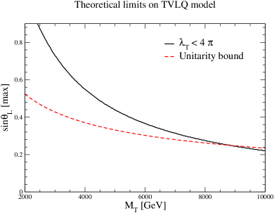
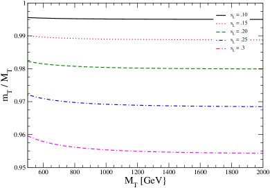
Figure 1: LHS: Upper limit on $s_{L}$ as a function of $M_{T}$ from perturbativity and unitarity. RHS: Relationship between the Lagrangian mass, $m_{\mathcal{T}}$, and the physical mass, $M_{T}$, for fixed $\sin\theta_{L}\equiv s_{L}$.

The relations of Eq. (9) can be inverted Cacciapaglia:2010vn :

$$m_{t}^{2} = {(\lambda_{t}^{2}+\lambda_{T}^{2})v^{2}\over 4}+{m_{\mathcal{T}}^{2}\over 2}\biggl{[}1-\sqrt{\biggl{(}1+{(\lambda_{t}^{2}+\lambda_{T}^{2})v^{2}\over 2m_{\mathcal{T}}^{2}}\biggr{)}^{2}-{2\lambda_{t}^{2}v^{2}\over m_{\mathcal{T}}^{2}}}\biggr{]}$$

$$M_{T}^{2} = {m_{\mathcal{T}}^{2}\over m_{t}^{2}}\biggl{(}{\lambda_{t}^{2}v^{2}\over 4}\biggr{)}$$

$$s_{L} = {\lambda_{T}v\over\sqrt{2}m_{\mathcal{T}}}{1\over\sqrt{(1-{m_{t}^{2}\over m_{\mathcal{T}}^{2}})^{2}+{\lambda_{T}^{2}v^{2}\over 2m_{\mathcal{T}}^{2}}}}\,.$$ (11)

In our phenomenological studies we will switch between Lagrangian parameters and the physical parameters to illustrate various points. We remind the reader that the physical masses are $m_{t}$ and $M_{T}$ with $m_{t}<<M_{T}$ and that $m_{\mathcal{T}}$ is the Lagrangian parameter.

The oblique parameters place stringent limits on the parameters of the TVLQ. In Fig. 2, we update the results of Ref. Chen:2017hak , include the global fit results of Ref. Dawson:2020oco and compare with the direct search limits from $T\bar{T}$ pair production ATLAS:2018ziw ; cms_2018 (which are independent of $s_{L}$). We also show a comparison of current searches with projections for HL-LHC and FCC-hh and note that the HL-LHC will be sensitive to $M_{T}\sim 1.7~{}\textrm{TeV}$, while the FCC-hh can probe up to $\sim 6~{}\textrm{TeV}$ Liu_2019 ; Yang:2021btv .

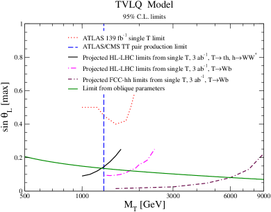
Figure 2: LHC $95\%$ exclusion limits on TVLQ masses from single $T$ production with $T\rightarrow ht,Zt$ as a function of $s_{L}$ ATLAS_singt (red dotted line) and limits from $T{\bar{T}}$ production with $T\rightarrow th,Zt,Wb$ ATLAS:2018ziw ; cms_2018 (blue dashed), projected limits from single $T$ production at HL-LHC with $T\rightarrow th,h\rightarrow WW^{*}$ Liu_2019 , (black solid), projected limits at HL-LHC from single $T$ production with $T\rightarrow Wb$ Yang:2021btv (magenta dot-dashed), and projected limits at FCC-hh ($\sqrt{S}=100\,\textrm{TeV}$) from single $T$ production with $T\rightarrow Wb$ Yang:2021btv (purple long dot-dashed). The region above the curves is excluded.

III Matching to SMEFT at dimension-$8$

In this section, we consider the $M_{T}\rightarrow\infty$ limit of the TVLQ model and perform the tree-level matching to the SMEFT, extending the dimension-$6$ results Aguila_2000 ; Chen:2014xwa ; Buras_2011 to dimension-$8$. Since the full UV model depends on only three unknown parameters, it is particularly simple. We use the covariant derivative expansion Gaillard:1985uh ; Henning:2014wua to integrate the heavy $T$ out of the theory and generate the effective operators at dimension-$6$ and dimension-$8$. The resulting Lagrangian involving the SM-like top quark, $t$, is,

$$\mathcal{L}_{t}\equiv\mathcal{L}_{\textrm{kin}}+\mathcal{L}_{Y}+\mathcal{L}_{6}+\mathcal{L}_{8}\,,$$ (12)

where,

$$\mathcal{L}_{\textrm{kin}} = i{\overline{\psi}}_{L}\not{D}\psi_{L}+i{\overline{t}}_{R}\not{D}t_{R}$$

$$= {i\over 2}\biggl{[}{\overline{\psi}}_{L}(\not{D}\psi_{L})-({\overline{\psi}}_{L}\overleftarrow{\not{D}})\psi_{L}\biggr{]}+i{\overline{t}}_{R}\not{D}t_{R}$$

$$\mathcal{L}_{Y} = -\lambda_{t}{\overline{\psi}}_{L}{\tilde{H}}t_{R}+\textrm{h.c.}$$

$$\mathcal{L}_{6} = \frac{i}{2}{\lambda_{T}^{2}\over m_{\mathcal{T}}^{2}}{\overline{\psi}}_{L}{\tilde{H}}\not{D}({\tilde{H}}^{\dagger}\psi_{L})+\textrm{h.c.}$$

$$\mathcal{L}_{8} = -\frac{i}{2}{\lambda_{T}^{2}\over m_{\mathcal{T}}^{4}}{\overline{\psi}}_{L}{\tilde{H}}\not{D}^{3}({\tilde{H}}^{\dagger}\psi_{L})+\textrm{h.c.},$$ (13)

where $\not{D}\equiv\gamma^{\mu}D_{\mu}$. The covariant derivative $D_{\mu}$ is defined as $\partial_{\mu}-i\frac{g}{2}YB_{\mu}-ig_{W}\tau_{a}W^{a}_{\mu}-ig_{s}T_{a}G^{a}_{\mu}$, with hypercharge $Y$, $SU(2)$ generators $\tau_{a}$, and $SU(3)$ generators $T_{a}$. The dimension-$6$ term, $L_{6}$, generates a non-standard normalization for the top quark kinetic energy term after electroweak symmetry breaking and the expansion of the Higgs field around its vev, so we make the gauge invariant field redefinition Criado:2018sdb ; Brivio:2017bnu ,

$$\psi_{L,i} \rightarrow \biggl{(}\psi_{L,i}-{\lambda_{T}^{2}\over 2m_{\mathcal{T}}^{2}}(\tilde{H}^{\phantom{\dagger}}_{i}\tilde{H}^{\dagger}_{j})\psi_{L,j}\biggr{)}\,,$$ (14)

where $i,j$ are $SU(2)$ indices. This brings the top quark kinetic energy into the canonical form.

Dimension-$6$
$O_{Ht}^{1,(6)}$	$(\mbox{${H^{\dagger}i\,\raisebox{5.69054pt}{\boldmath${}^{\leftrightarrow}$}D_{\mu}\,H}$})(\bar{\psi}_{L}\gamma^{\mu}\psi_{L})$
$O_{Ht}^{3,(6)}$	$(\mbox{${H^{\dagger}i\,\raisebox{5.69054pt}{\boldmath${}^{\leftrightarrow}$}D_{\mu}^{\,a}\,H}$})(\bar{\psi}_{L}\tau^{a}\gamma^{\mu}\psi_{L})$
$O_{tH}^{(6)}$	$(H^{\dagger}H){\overline{\psi}}_{L}{\tilde{H}}t_{R}$
Dimension-$8$
$O_{quH^{5}}^{(8)}$	$(H^{\dagger}H)^{2}{\overline{\psi}}_{L}{\tilde{H}}t_{R}$

Table 1: Operators appearing in Eq. (15) where $\psi_{L}$ is the $(t,b)$ doublet, $H^{\dagger}\raisebox{5.69054pt}{\boldmath${}^{\leftrightarrow}$}D_{\mu}\,H\equiv H^{\dagger}D_{\mu}H-(D_{\mu}H^{\dagger})H$ and $H^{\dagger}\raisebox{5.69054pt}{\boldmath${}^{\leftrightarrow}$}D_{\mu}^{a}\,H\equiv H^{\dagger}D_{\mu}\sigma^{a}H-(D_{\mu}H^{\dagger}\sigma^{a})H$.

After making the field redefinition of Eq. (14),

$$i{\overline{\psi}}_{L}\not{D}\psi_{L}+\mathcal{L}_{6} \rightarrow i{\overline{\psi}}_{L}\not{D}\psi_{L}+{i\lambda_{T}^{2}\over 2m_{\mathcal{T}}^{2}}\biggl{[}({\overline{\psi}}_{L}{\tilde{H}})(\not{D}{\tilde{H}}^{\dagger})\psi_{L}-{\overline{\psi}}_{L}(\not{D}{\tilde{H}}){\tilde{H}}^{\dagger}\psi_{L}\biggr{]}+\delta\mathcal{L}_{8a}$$

$$= i{\overline{\psi}}_{L}\not{D}\psi_{L}+{i\lambda_{T}^{2}\over 4m_{\mathcal{T}}^{2}}\biggl{[}({\overline{\psi}}_{L}\gamma^{\mu}\psi_{L})\biggl{(}H^{\dagger}D_{\mu}H-(D_{\mu}H^{\dagger})H\biggr{)}$$

$$-({\overline{\psi}}_{L}\gamma^{\mu}\tau^{a}\psi_{L})\biggl{(}H^{\dagger}\tau^{a}D_{\mu}H-(D_{\mu}H^{\dagger})\tau^{a}H\biggr{)}\biggr{]}+\delta\mathcal{L}_{8a}$$

$$= i{\overline{\psi}}_{L}\not{D}\psi_{L}+{i\lambda_{T}^{2}\over 4m_{\mathcal{T}}^{2}}\biggl{[}O_{Ht}^{1,(6)}-O_{Ht}^{3,(6)}\biggr{]}+\delta\mathcal{L}_{8a}$$

$$\delta\mathcal{L}_{8a} \equiv {i\lambda_{T}^{4}\over 8m_{\mathcal{T}}^{4}}\biggl{[}3\not{D}({\overline{\psi}}_{L}{\tilde{H}}){\tilde{H}}^{\dagger}{\tilde{H}}{\tilde{H}}^{\dagger}\psi_{L}+{\overline{\psi}}_{L}{\tilde{H}}{\tilde{H}}^{\dagger}(\not{D}{\tilde{H}}){\tilde{H}}^{\dagger}\psi_{L}+\textrm{h.c.}\biggr{]}$$

$$= {\lambda_{T}^{4}\over 8m_{\mathcal{T}}^{4}}\biggl{[}-3\lambda_{t}O_{quH^{5}}^{(8)}+3(H^{\dagger}H){\overline{\psi}_{L}}(i\not{D}{\tilde{H}}){\tilde{H}}^{\dagger}\psi_{L}+{\overline{\psi}}_{L}{\tilde{H}}{\tilde{H}}^{\dagger}(i\not{D}{\tilde{H}}){\tilde{H}}^{\dagger}\psi_{L}+\textrm{h.c.}\biggr{]}$$

$$\mathcal{L}_{Y} \rightarrow -\lambda_{t}{\overline{\psi}}_{L}{\tilde{H}}t_{R}\biggl{[}1-{\lambda_{T}^{2}\over 2m_{\mathcal{T}}^{2}}(H^{\dagger}H)\biggr{]}+\textrm{h.c.}$$ (15)

$$\equiv \biggl{[}-\lambda_{t}{\overline{\psi}}_{L}{\tilde{H}}t_{R}+{\lambda_{t}\lambda_{T}^{2}\over 2m_{\mathcal{T}}^{2}}O_{tH}^{(6)}+\textrm{h.c.}\biggr{]}\,,$$

where in the second line of Eq. (15), $SU(2)$ identities are used to put the dimension-6 contributions in a standard form. Note that Eq. (15) contains dimension-$8$ interactions in addition to those of the dimension-$8$ operator of $\mathcal{L}_{8}$. Repeated use of the SM equations of motion on the dimension-$8$ term, $\delta\mathcal{L}_{8a}$, yields the second line of the expression for $\delta L_{8a}$ in Eq. (15). We have not simplified the dimension-8 contributions with derivatives on the Higgs doublet, since it is straightforward to use FeynRules Degrande_2012 ; Alloul_2014 to determine the needed interactions for a given application. The operators are defined in Tab. 1 using the bases of Refs. Grzadkowski_2010 ; Murphy:2020ab .

We simplify the dimension-$8$ operator of Eq. (13) to extract the term contributing to the top quark Yukawa interaction,

$$\mathcal{L}_{8} \rightarrow {\lambda_{t}^{3}\lambda_{T}^{2}\over 2m_{\mathcal{T}}^{4}}(H^{\dagger}H)^{2}\biggl{(}{\overline{\psi}}_{L}{\tilde{H}}t_{R}+\textrm{h.c.}\biggr{)}+{\rm terms~{}with~{}derivatives~{}on}~{}{\tilde{H}}~{}{\rm or}~{}{\tilde{H}}^{\dagger}$$ (16)

$$\equiv \biggl{(}{\lambda_{t}^{3}\lambda_{T}^{2}\over 2m_{\mathcal{T}}^{4}}(H^{\dagger}H)^{2}O_{quH^{5}}^{(8)}+\textrm{h.c.}\biggr{)}+\delta\mathcal{L}_{8b}\,,$$

where the complete expression for $\delta\mathcal{L}_{8b}$ can be found in the supplemental material. The contribution to $\delta\mathcal{L}_{8b}$ that is proportional to the strong coupling, $g_{s}$, is given in Appendix A and the momentum dependence of the dimension-8 operators is clearly seen.

The complete SMEFT Lagrangian generated from the TVLQ model to dimension-$8$ involving the top quark written in terms of the Lagrangian parameters is,

$$\mathcal{L} \equiv \mathcal{L}_{4}^{\prime}+\mathcal{L}_{6}^{\prime}+\mathcal{L}_{8}^{\prime}$$

$$\mathcal{L}_{4}^{\prime} = {\overline{\psi}}_{L}(i\not{D})\psi_{L}+{\overline{t}_{R}(i\not{D})t_{R}}-(\lambda_{t}{\overline{\psi}}_{L}{\tilde{H}}t_{R}+\textrm{h.c.})$$

$$\mathcal{L}_{6}^{\prime} = \biggl{(}{\lambda_{t}\lambda_{T}^{2}\over 2m_{\mathcal{T}}^{2}}O_{tH}^{(6)}+\textrm{h.c.}\biggr{)}+{\lambda_{T}^{2}\over 4m_{\mathcal{T}}^{2}}\biggl{(}O_{Ht}^{1,(6)}-O_{Ht}^{3,(6)}\biggr{)}$$

$$\mathcal{L}_{8}^{\prime} = {\lambda_{t}\lambda_{T}^{2}\over 8m_{\mathcal{T}}^{4}}(4\lambda_{t}^{2}-3\lambda_{T}^{2})O_{quH^{5}}^{(8)}+\delta\mathcal{L}_{8b}+\textrm{h.c.}$$ (17)

We note that changing the input parameters from ($\lambda_{t}$, $\lambda_{T}$, $m_{\mathcal{T}}$) to ($m_{t}$, $M_{T}$, $s_{L}$) using Eq. (8) re-arranges the counting in terms of inverse powers of the heavy mass Brehmer:2015rna . Ref. Brehmer:2015rna argues that replacing the Lagrangian mass, $m_{\mathcal{T}}$, with the physical mass, $M_{T}$, improves the agreement between the SMEFT predications and those of the corresponding UV complete model in many cases. A similiar effect is found in the EFT limit of the 2HDM Egana-Ugrinovic:2015vgy ; B_lusca_Ma_to_2017 .

The terms contributing to the SMEFT relationship between the top mass and Higgs top Yukawa coupling are,

$$\mathcal{L} \sim -\lambda_{t}{\overline{\psi}}_{L}{\tilde{H}}t_{R}+{C_{tH}^{(6)}\over m_{\mathcal{T}}^{2}}O_{tH}^{(6)}+{C_{quH^{5}}^{(8)}\over m_{\mathcal{T}}^{4}}O_{quH^{5}}^{(8)}+\textrm{h.c.}$$ (18)

with,

$$C_{tH}^{(6)}={\lambda_{t}\lambda_{T}^{2}\over 2}\,,\qquad C_{quH^{5}}^{(8)}={\lambda_{t}\lambda_{T}^{2}\over 8}(4\lambda_{t}^{2}-3\lambda_{T}^{2})\,.$$ (19)

It is interesting to study the behaviors of $C_{tH}^{(6)}$ and $C_{quH^{5}}^{(8)}$ using the relationships of Eq. (9) and expanding in powers of ${1/m_{\mathcal{T}}}$ keeping the top quark mass fixed to its physical value. Note that keeping the top quark mass fixed rearranges the counting, as does alternatively using $s_{L}$ and $M_{T}$ as inputs. To ${\cal{O}}({1/m_{\mathcal{T}}^{4}})$,

$$\lambda_{t} = {\sqrt{2}m_{t}\over v}\biggl{\{}1+{\lambda_{T}^{2}v^{2}\over 4m_{\mathcal{T}}^{2}}+{\lambda_{T}^{2}v^{2}m_{t}^{2}\over 4m_{\mathcal{T}}^{4}}-{\lambda_{T}^{4}v^{4}\over 32m_{\mathcal{T}}^{4}}\biggr{\}}$$

$$\rightarrow {\sqrt{2}m_{t}\over c_{L}v}\biggl{\{}1-s_{L}^{2}{m_{t}^{2}\over m_{\mathcal{T}}^{2}}-s_{L}^{4}{m_{t}^{4}\over 4m_{\mathcal{T}}^{4}}\biggr{\}}$$

$${\overline{C}}_{6} \equiv {C_{tH}\over m_{\mathcal{T}}^{2}}$$

$$\rightarrow {2m_{t}s_{L}^{2}\over\sqrt{2}c_{L}^{3}v^{3}}\biggl{(}1-{(s_{L}^{2}+4)m_{t}^{2}\over 2m_{\mathcal{T}}^{2}}-{(s_{L}^{4}-8s_{L}^{2}-8)m_{t}^{4}\over 8m_{\mathcal{T}}^{4}}\biggr{)}$$

$${\overline{C}}_{8} \equiv {C_{quH^{5}}\over m_{\mathcal{T}}^{4}}$$ (20)

$$\rightarrow {m_{t}\over\sqrt{2}}{s_{L}^{2}\over c_{L}^{5}v^{5}}\biggl{\{}-3s_{L}^{2}+{m_{t}^{2}\over 2m_{\mathcal{T}}^{2}}(3s_{L}^{4}+24s_{L}^{2}+8)+{m_{t}^{4}\over 8m_{\mathcal{T}}^{4}}(3s_{L}^{6}-48s_{L}^{4}-192s_{L}^{2}-64)\biggr{\}}\,.$$

The naive scalings, ${\overline{C}}_{6}\sim{1/m_{\mathcal{T}}^{2}}$ and ${\overline{C}}_{8}\sim{1/m_{\mathcal{T}}^{4}}$ are modified by terms of ${\cal{O}}(s_{L}^{2}x)$ when using the physical parameters.

Expanding Eq. (18) to linear order in the Higgs field, we define the top Yukawa, $Y_{t}^{(8)}$, as usual

$$\mathcal{L}\sim-{Y_{t}^{(8)}\over\sqrt{2}}{\overline{t}}_{L}t_{R}h+\textrm{h.c.}$$ (21)

where the superscript $8$ denotes the inclusion of the dimension-$8$ contributions. We initially fix $m_{t}$ (the physical top quark mass), $\lambda_{T}$ and $m_{\mathcal{T}}$,

$$Y_{t}^{(8)} = {\lambda_{t}}-{3v^{2}\over 2}{\overline{C}}_{6}-{5v^{4}\over 4}{\overline{C}}_{8}$$ (22)

$$= {m_{t}\sqrt{2}\over v}\biggl{\{}1-{\lambda_{T}^{2}v^{2}\over 2m_{\mathcal{T}}^{2}}-{m_{t}^{2}v^{2}\lambda_{T}^{2}\over m_{\mathcal{T}}^{4}}+{\lambda_{T}^{4}v^{4}\over 4m_{\mathcal{T}}^{4}}\biggr{\}}\,.$$

Retaining only the dimension-$6$ terms in the Lagrangian,

$$Y_{t}^{(6)} = {\lambda_{t}}-{3v^{2}\over 2}{\overline{C}}_{6}$$ (23)

$$= {m_{t}\sqrt{2}\over v}\biggl{\{}1-{\lambda_{T}^{2}v^{2}\over 2m_{\mathcal{T}}^{2}}\biggr{\}}+{\cal{O}}\biggl{(}{1\over m_{\mathcal{T}}^{4}}\biggr{)}\,.$$

In Eqs. (22) and (23), the SM is recovered in the ${\lambda_{T}^{2}/m_{\mathcal{T}}^{2}}\rightarrow 0$ limit, which corresponds to the $s_{L}\rightarrow 0$ limit. The choice to use $m_{t}$ as an input introduces terms of ${\cal{O}}\big{(}{\lambda_{T}^{4}/m_{\mathcal{T}}^{4}}\big{)}$ in $Y_{t}^{(6)}$ due to the interdependence of the parameters.

In the small $s_{L}$ limit,

$$Y_{t}^{(8)} \rightarrow {m_{t}\sqrt{2}\over v}\biggl{\{}1-s_{L}^{2}+{3s_{L}^{2}m_{t}^{4}\over m_{\mathcal{T}}^{4}}\biggr{\}}$$

$$Y_{t}^{(6)} \rightarrow {m_{t}\sqrt{2}\over v}\biggl{\{}1-s_{L}^{2}+{5s_{L}^{2}m_{t}^{2}\over 2m_{\mathcal{T}}^{2}}-{3s_{L}^{2}m_{t}^{4}\over 2m_{\mathcal{T}}^{4}}\biggr{\}}\,.$$ (24)

We see that the SM limit is only recovered in the $s_{L}\rightarrow 0$ limit, consistent with the decoupling discussion in the previous section. Fig. 3 shows the effect of including the dimension-$8$ terms on the top quark Yukawa coupling and we see that it is typically less than a few percent for $500~{}\textrm{GeV}<m_{\mathcal{T}}<1~{}\textrm{TeV}$.

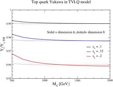
Figure 3: Top quark Yukawa coupling normalized to the SM top quark Yukawa when dimension-$8$ contributions are included ($Y_{t}^{(8)}$) and when only dimension-$6$ terms are included ($Y_{t}^{(6)}$).

IV Phenomenology

We are now in a position to investigate the numerical effects of including the dimension-8 terms in the SMEFT analysis of the TVLQ and in the comparison between SMEFT and the UV complete model. As an example of the possible impact of the dimension-8 contributions, we consider $t\bar{t}h$ production at the $13~{}\textrm{TeV}$ LHC. In addition to the SM cross section, $\text{d}\sigma_{\textrm{SM}}$, we consider various SMEFT expansions:

$$\text{d}\sigma_{\textrm{int}} \sim \int(\text{d}{\rm PS})\biggl{\{}|\mathcal{A}_{\textrm{SM}}|^{2}+{2\over\Lambda^{2}}\textrm{Re}\biggl{(}\sum C_{i}^{(6)}\mathcal{A}_{i}^{(6)}\mathcal{A}_{\textrm{SM}}^{*}\biggr{)}\biggr{\}}$$

$$\text{d}\sigma_{6} \sim \int(\text{d}{\rm PS})\biggl{\{}|\mathcal{A}_{\textrm{SM}}|^{2}+{2\over\Lambda^{2}}\textrm{Re}\biggl{(}\sum C_{i}^{(6)}\mathcal{A}_{i}^{(6)}\mathcal{A}_{\textrm{SM}}^{*}\biggr{)}+{1\over\Lambda^{4}}\textrm{Re}\biggl{(}\sum_{i,j}C_{i}^{(6)}C_{j}^{(6)*}\mathcal{A}_{i}^{(6)}\mathcal{A}_{j}^{(6)~{}*}\biggr{)}\biggr{\}}$$

$$\text{d}\sigma_{8} \sim \int(\text{d}{\rm PS})\biggl{\{}|\mathcal{A}_{\textrm{SM}}|^{2}+{2\over\Lambda^{2}}\textrm{Re}\biggl{(}\sum C_{i}^{(6)}\mathcal{A}_{i}^{(6)}\mathcal{A}_{\textrm{SM}}^{*}\biggr{)}+{1\over\Lambda^{4}}\textrm{Re}\biggl{(}\sum_{i,j}C_{i}^{(6)}C_{j}^{(6)*}\mathcal{A}_{i}^{(6)}\mathcal{A}_{j}^{(6)~{}*}\biggr{)}$$ (25)

$$\quad+{2\over\Lambda^{4}}\textrm{Re}\biggl{(}\sum_{i}C_{i}^{(8)}\mathcal{A}_{i}^{(8)}\mathcal{A}_{\textrm{SM}}^{*}\biggr{)}\biggr{\}}\,.$$

In particular, $\text{d}\sigma_{6}$ and $\text{d}\sigma_{8}$ are of the same order in $1/\Lambda^{4}$ and the difference between the two is a measure of the importance of the dimension-8 terms. In our numerical studies, we will always take $\Lambda=m_{\mathcal{T}}$.

The rescaling of the top Yukawa coupling at dimension-8 will give only a small difference from the dimension-6 result as demonstrated in Fig. 3. However, the dimension-8 terms introduce a momentum dependence into the $t\bar{t}h$ and $t\bar{t}hg$ vertices, as well as the $tbW$ and $tbWh$ vertices. The Feynman rules relevant for the $t{\bar{t}}h$ process are given in Appendix A. Note that, since there is never more than one covariant derivative operating on the top quark at dimension-$8$, the TVLQ model only generates new operators with a single gluon field. We use FeynRules Christensen_2009 ; Alloul_2014 to generate the Feynman rules including the dimension-8 terms and use the resulting UFO Degrande_2012 file with MadGraph5 and the default dynamical scale choice to generate events. For all our simulations, we set $m_{t}=172\,\textrm{GeV}$, $m_{h}=125\,\textrm{GeV}$, $m_{Z}=91.1876\,\textrm{GeV}$, $G_{F}=1.16637\times 10^{-5}$, and $\alpha=1/127.9$, so that $m_{W}$ is computed to be $79.82436\,\textrm{GeV}$ at tree level in the MadGraph5 code. We use the NNPDF23 LO PDF set with $\alpha_{s}=0.119$. The complete set of interactions can be found using the FeynRules module contained in the supplemental materials.

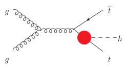
Figure 4: Sample Feynman diagrams contributing to $gg\rightarrow t\bar{t}h$ including dimension-$8$ operators. The blobs represent the effects of the dimension-$8$ operators for the center and right-handed diagrams, while the left-most diagram (red blob) receives contributions from both dimension-$6$ and dimension-$8$ operators. Similar diagrams with $q\bar{q}$ initial states are not shown, but included in our computations.

We begin by considering the $t\bar{t}h$ process without decays. Some sample diagrams are shown in Fig. 4. There are two effects from the higher dimension operators. The first is the rescaling of the $t\bar{t}h$ Yukawa interaction. This does not lead to any momentum-dependent effects in the $gg\to t\bar{t}h$ process, but due to the small contributions from the $q\bar{q}\to t\bar{t}h$ sub-process, where the $h$ couples to an intermediate $Z$ boson, which are not rescaled by the top Yukawa, there are very small kinematic effects in the total cross section at the $\lesssim 1\%$ level. The second effect, which first arises at dimension-$8$, is interactions that are enhanced by an energy factor, $\sim s$ (with $s$ the partonic center of mass energy), relative to the SM contributions, both in the $t\bar{t}h$ and $t\bar{t}hg$ effective vertices. However, these $s$-enhanced contributions are proportional to a difference in the projection operators, $(P_{R}-P_{L})$ (c.f. Eq. (27)), and the enhancement is therefore averaged out in the helicity-blind production of on shell tops from QCD production. The resulting distributions for $t\bar{t}h$ production without decays are therefore essentially flat in various kinematic observables, and roughly consistent with an overall rescaling of the cross section by the modified top Yukawas in Eqs. (22) and (23).

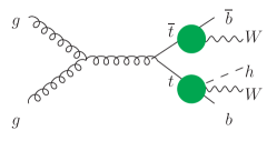
Figure 5: Sample diagrams contributing to $gg\rightarrow b{\overline{b}}W^{+}W^{-}h$. The green blob represents the insertion of dimension-$6$ operators, while the red blob represents both dimension-$6$ and dimension-$8$ operators. Similar diagrams with $q\bar{q}$ initial states are not shown, but included in our computations.

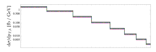
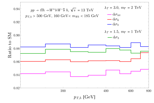
Figure 6: The distribution for $W^{+}W^{-}b\bar{b}h$ production with intermediate top quarks in bins of the Higgs $p_{T,h}$. The top panel shows the distribution for the SM (black), and for the TVLQ point with $\lambda_{T}=3.0$, $m_{\cal T}=2\,\textrm{TeV}$, matched to various orders in the SMEFT, as in Eq. (25), with the magenta, red and blue curves representing $\text{d}\sigma_{\textrm{int}}$, $\text{d}\sigma_{6}$ and $\text{d}\sigma_{8}$, respectively. The results for $\text{d}\sigma_{8}$ with $\lambda_{T}=1.5$ and $m_{\cal T}=1\,\textrm{TeV}$ are shown in green.

We next consider $t\bar{t}h$ production with the tops decayed to the final state $b\bar{b}W^{+}W^{-}h$. We generate events in this final state from all tree level diagrams including intermediate top quarks to exclude pure electroweak production of $W$ and $b$ pairs. This includes contributions from a number of diagrams which cannot be factorized into $t\bar{t}h$ production times decay. One example of such a diagram is shown in the right-hand side of Fig. 5. There are also contributions that are not proportional to the top Yukawa coupling, where the Higgs instead couples to the $W$ bosons or bottom quarks.

We compute the cross section for $pp\to b\bar{b}W^{+}W^{-}h$ with intermediate top quarks using our FeynRules implementation, and plot the result in bins of $p_{T,h}$ in Fig. 6. We show results both for the SM, and with the SMEFT matched with $\lambda_{T}=3.0$ and $m_{\mathcal{T}}=2\,\textrm{TeV}$, corresponding to a mixing angle $\sin\theta_{L}\sim 0.25$. We note that such large values of the mixing angle are excluded by fits to the oblique parameters (see Fig. 2) — we choose such a large point to make the kinematic effects that arise at different orders in the SMEFT expansion clear. To focus on the effects on $t\bar{t}h$ production, we impose a cut on the $W$ boson and $b$ quark system, requiring it to be near the top quark mass shell: $160\,\textrm{GeV}<m_{Wb}<185\,\textrm{GeV}$. We utilize the charge information of the $W$ and $b$ particles in performing this cut, assuming that they can be properly assigned to the correct top quark in a true experimental analysis, e.g., if they are all identified in a single large-radius top jet.

Including the full $b\bar{b}W^{+}W^{-}h$ final state changes the expectations from $t\bar{t}h$ production without decays significantly. The diagrams where the Higgs is coupled to a $W$ boson or $b$ quark are not proportional to the top Yukawa, and therefore are not rescaled by the corrections to the top Yukawa as the bulk of the cross section is in the un-decayed case. This leads to a growth in the cross section for large $p_{T,h}$ even at the dimension-6 level, and a change in the overall rate that is significantly different from a naive rescaling. At dimension-8, there are non-factorizable contributions with $thWb$ vertices, which have one fewer propagator than the SM-like diagrams, and as a result, $s$-enhanced effects relative to the Standard Model. Finally, since the tops decay via their $SU(2)_{L}$ interactions, the effective operators proportional to $(P_{R}-P_{L})$ discussed above will no longer be averaged out, and can therefore lead to additional effects at high $p_{T,h}$ as well. All of these effects in the amplitudes compete, and interfere with one another.

The resulting effects in Fig. 6 show that the kinematic effects apparent at dimension-6 are nearly washed out at dimension-8, and the distribution is almost flat. We emphasize that, while the overall distribution is roughly flat in $p_{T,h}$, due to a combination of different effects that arise at different orders in the EFT expansion, the overall rate is different than that expected by rescaling the SM cross section by the modified top Yukawa. Note also that the size of the contributions from the dimension-8 operators are similar to the size of the dimension-6 squared terms relative to the interference contribution alone.

We also include in Fig. 6 a curve in green, showing the results for matching up to dimension-8 with $\lambda_{T}=1.5$ and $m_{\mathcal{T}}=1\,\textrm{TeV}$. These values are chosen such that the effects at dimension-6 in the SMEFT, which all scale as $\lambda_{T}^{2}/m_{\mathcal{T}}^{2}$, are precisely the same as for $\lambda_{T}=3.0$, $m_{\mathcal{T}}=2\,\textrm{TeV}$. At dimension-8, however, there are effects that break this scaling (c.f. Eqs. (22) and (27) – (29)), and we see that indeed, the dimension-8 curve in green is different than the curve in blue.

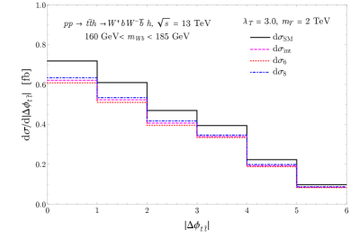
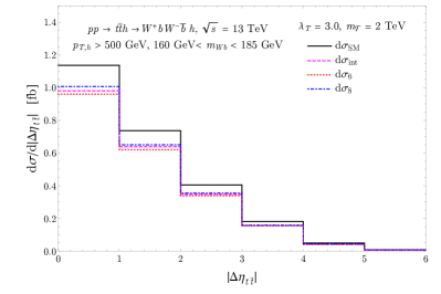
Figure 7: The distribution for $W^{+}W^{-}b\bar{b}h$ production with intermediate top quarks in bins of $|\Delta\phi_{t\bar{t}}|$ (left) and $|\Delta\eta_{t\bar{t}}|$ (right), for events with $p_{T,h}>500\,\textrm{GeV}$, matched at various orders in the SMEFT expansion for $\lambda_{T}=3.0$, $m_{\mathcal{T}}=2\,\textrm{TeV}$. The black solid, magenta dashed, red dotted, and blue dot-dashed curves show the results for $\text{d}\sigma_{\textrm{SM}}$, $\text{d}\sigma_{\textrm{int}}$, $\text{d}\sigma_{6}$ and $\text{d}\sigma_{8}$, respectively.

In Fig. 7, we show the distributions for $t\bar{t}h$ production including the full $b\bar{b}W^{+}W^{-}h$ final state in bins of $|\Delta\phi_{t\bar{t}}|$ and $|\Delta\eta_{t\bar{t}}|$, after placing a cut on the Higgs $p_{T,h}>500\,\textrm{GeV}$. We see there are no kinematic effects in these distributions at any order in the SMEFT expansion, other than the rescaling consistent with the results in Fig. 6.

Finally, we comment on the size of the dimension-8 effects for parameters that are not experimentally excluded. We take $\lambda_{T}=1.5$, $m_{\mathcal{T}}=2\,\textrm{TeV}$, corresponding to a mixing angle $\sin\theta_{L}=0.13$, which is near the edge of the region allowed by the oblique parameter fits shown in Fig. 2. For these parameters, the effects of the dimension-8 terms included in $\text{d}\sigma_{8}$ are very small: $\lesssim\mathcal{O}(1\%)$ of the SM cross section. The effects of the $\mathcal{O}(1/\Lambda^{4})$ terms in $\text{d}\sigma_{6}$ are of similar size. There are small kinematic effects, but the total rate is quite similar to what one expects from a naive rescaling of the cross section by $(Y_{t}^{(6)})^{2}$. We conclude that the effects of the $\mathcal{O}(1/\Lambda^{4})$ terms are too small to affect constraints on the TVLQ model at the LHC from $tth$ production.

V Discussion

We have implemented the complete dimension-8 set of operators contributing to the tree level process, $pp\rightarrow t{\overline{t}}h$, in a model with a charge-$2/3$ vector-like quark. When the decays of the top quark are not included, the results are almost entirely given by the rescaling of the top quark Yukawa coupling. The decays of the top quark introduce a momentum dependence due primarily to the presence of non-factorizable $tbWh$ vertices. These effects create a difference of less than ${\cal O}(2\%)$ at high $p_{T,h}$ between the square of the dimension-6 contributions and the result with the dimension-8 contributions included.

The example we have considered is particularly simple, since the input parameters are not rescaled at tree level to dimension-8. It would be of interest to consider the effects of a more complicated model which generates tree level rescaling of the input parameters at dimension-8. The results of Refs. Corbett:2021iob ; Corbett:2021eux suggest that the dimension-8 contributions may play a more significant role in such scenarios.

The UFO and FeynRules model files used to generate the TVLQ dimension-8 effects are included as supplemental material.

Appendix A Dimension-8 Interactions

The following terms in the tree-level dimension-$8$ Lagrangian, $\mathcal{L}_{8}^{\prime}$, contain non-SM gluon couplings:

$$\mathcal{L}_{8,g} = i\frac{\lambda_{T}^{2}}{m_{\mathcal{T}}^{4}}(\bar{\psi}_{L}D^{\mu}\tilde{H})\gamma_{\mu}(D^{\nu}\tilde{H}^{\dagger}D_{\nu}\psi_{L})+i\frac{\lambda_{T}^{2}}{m_{\mathcal{T}}^{4}}(\bar{\psi}_{L}\tilde{H})\gamma_{\mu}(D^{\mu}D^{\nu}\tilde{H}^{\dagger}D_{\nu}\psi_{L})$$ (26)

$$- i\frac{\lambda_{T}^{2}}{m_{\mathcal{T}}^{4}}(\bar{\psi}_{L}\tilde{H})\gamma_{\mu}(D^{\nu}D^{\mu}\tilde{H}^{\dagger}D_{\nu}\psi_{L})-\frac{\lambda_{t}\lambda_{T}^{2}}{m_{\mathcal{T}}^{4}}(H^{\dagger}H)\bar{t}_{R}(D^{\mu}\tilde{H}^{\dagger}D_{\mu}\psi_{L})+\textrm{h.c.},$$

where indices are contracted implicitly such that terms in parentheses are $SU(2)$ singlets. The $t{\overline{t}}h$ interactions that are needed for the tree level process are (with all momenta outgoing),

$$t(p_{1}){\overline{t}}(p_{2})h(p_{h}) = -i{Y_{t}^{(8)}\over\sqrt{2}}+i{\lambda_{T}^{2}vm_{t}\over 4m_{\mathcal{T}}^{4}}(p_{1}-p_{2})\cdot p_{h}(P_{R}-P_{L})$$

$$t(p_{1}){\overline{t}}(p_{2})h(p_{h})g^{A\mu}(p_{g}) = ig_{s}{\lambda_{T}^{2}vm_{t}\over 2m_{\mathcal{T}}^{4}}p_{h}^{\mu}T^{A}(P_{R}-P_{L})$$ (27)

where $P_{L,R}\equiv{1\over 2}(1\mp\gamma_{5})$ and $Y_{t}^{(8)}$ is as given in Eq. (22).

The following are the electroweak couplings of the top quark expanded to dimension eight that occur in the $t{\overline{t}}h,~{}t\rightarrow Wb$ process:

$$b(p_{b}){\overline{t}}(p_{t})W^{+\mu}(p_{W}) = i\frac{g_{W}}{\sqrt{2}}\gamma^{\mu}P_{L}\biggl{[}1-\frac{v^{2}\lambda_{T}^{2}}{4{m_{\mathcal{T}}}^{2}}+\frac{v^{2}\lambda_{T}^{2}}{32{m_{\mathcal{T}}}^{4}}\biggl{(}3v^{2}\lambda_{T}^{2}+8(m_{t}^{2}-p_{t}^{2}+p_{b}^{2})\biggr{)}\biggr{]}$$ (28)

$$-i\frac{g_{W}v^{2}\lambda_{T}^{2}}{2\sqrt{2}{m_{\mathcal{T}}}^{4}}p_{b}^{\mu}P_{R}\biggl{[}m_{t}-\not{p_{W}}\biggr{]}$$

$$b(p_{b}){\overline{t}}(p_{t})W^{+\mu}(p_{W})h(p_{h}) = -\frac{ivg_{W}\lambda_{T}^{2}\gamma^{\mu}P_{L}}{2\sqrt{2}{m_{\mathcal{T}}}^{2}}\biggl{[}1+\frac{p_{h}\cdot p_{t}}{{m_{\mathcal{T}}}^{2}}+\frac{2p_{b}\cdot p_{W}}{{m_{\mathcal{T}}}^{2}}+\frac{p_{h}^{2}}{2{m_{\mathcal{T}}}^{2}}+\frac{p_{W}^{2}}{{m_{\mathcal{T}}}^{2}}+\frac{p_{h}\cdot p_{W}}{{m_{\mathcal{T}}}^{2}}$$ (29)

$$-\frac{3v^{2}\lambda_{T}^{2}}{4{m_{\mathcal{T}}}^{2}}-\frac{2m_{t}^{2}}{{m_{\mathcal{T}}}^{2}}-\frac{\not{p_{h}}\not{p_{W}}}{2{m_{\mathcal{T}}}^{2}}-{m_{t}\not{p_{h}}\over 2m_{\mathcal{T}}^{2}}\biggr{]}$$

$$+\frac{ivg_{W}\lambda_{T}^{2}P_{R}}{2\sqrt{2}{m_{\mathcal{T}}}^{4}}\biggl{[}p_{b}^{\mu}\biggl{(}\not{p_{h}}+2\not{p_{W}}-3m_{t}\biggr{)}-p_{h}^{\mu}\biggl{(}\not{p_{h}}+\not{p_{W}}-m_{t}\biggr{)}\biggr{]}$$

Appendix B $T$ Parameter in Effective Field Theory Language

The oblique parameter $\Delta{\cal{T}}$ has been calculated some time ago for the TVLQ model Dawson:2012di . It is instructive to revisit this calculation using an effective field theory framework delAguila:2016zcb and it is an example of the importance of including the one-loop matching in SMEFT calculations. The contributions to $\Delta{\cal{T}}$ from fermions with masses $m_{1}$ and $m_{2}$ can be expressed in terms of the function,

$$\theta_{+}(y_{1},y_{2}) = y_{1}+y_{2}-{2y_{1}y_{2}\over y_{1}-y_{2}}\log\biggl{(}{y_{1}\over y_{2}}\biggr{)}-2\biggl{(}y_{1}\log(y_{1})+y+2\log(y_{2})\biggr{)}$$ (30)

$$-2(y_{1}+y_{2}){1\over\epsilon}\biggl{(}{4\pi\mu^{2}\over M_{Z}^{2}}\biggr{)}^{\epsilon}\,,$$

where $y_{i}={m_{i}^{2}/M_{Z}^{2}}$ and $\mu$ is an arbitrary renormalization scale. Neglecting the $b$ quark mass and taking $m_{t}\gg M_{Z}$, the $t-b$ contribution to the SM is found from the diagrams of Fig. 8 with SM fermion-gauge boson couplings,

$${\cal{T}}_{\textrm{SM}} = {3\over 16\pi s_{W}^{2}c_{W}^{2}}y_{t}$$ (31)

with $c_{W}\equiv{M_{W}/M_{Z}}$.

Figure 8: Feynman diagrams contributing to the ${\cal{T}}$ parameter from SM fermions.

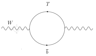
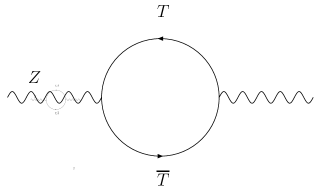
Figure 9: Feynman diagrams contributing to the ${\cal{T}}$ parameter from the heavy $TVLQ$ fermion, $T$.

At the UV scale (which here we take to be the physical mass of the TVLQ, $M_{T}$), we integrate out the contributions of the diagrams of Fig. 9 using the couplings from Ref. Chen:2017hak to obtain the contribution from heavy fermions, ${\cal{T}}_{H}$,

$${\cal{T}}_{H}(\mu) = T_{\textrm{SM}}s_{L}^{2}\biggl{(}\theta_{+}(y_{T},y_{b})-c_{L}^{2}\theta_{+}(y_{T},y_{t})-{1\over 2}\theta_{+}(y_{T},y_{T})\biggr{)}$$ (32)

$$= T_{\textrm{SM}}s_{L}^{2}\biggl{\{}s_{L}^{2}{M_{T}^{2}\over m_{t}^{2}}-c_{L}^{2}+{2c_{L}^{2}\over\epsilon}+2c_{L}^{2}\log\biggl{(}{M_{T}^{2}\over\mu^{2}}\biggr{)}\biggr{\}}$$

For the UV matching, the appropriate scale is $\mu=M_{T}$, giving the contribution,

$${\cal{T}}_{H}(M_{T}) = T_{\textrm{SM}}s_{L}^{2}\biggl{\{}s_{L}^{2}{M_{T}^{2}\over m_{t}^{2}}-c_{L}^{2}+{2c_{L}^{2}\over\epsilon}\biggr{\}}\,.$$ (33)

Eq. (33) exhibits the familiar decoupling requirement that $s_{L}^{2}M_{T}^{2}/m_{t}^{2}\ll 1$.

We identify,

$${\cal{T}}(\mu)=-{v^{2}\over 2\alpha}{C^{(6)}_{HD}(\mu)\over\Lambda^{2}}$$ (34)

where $O_{HD}=|H^{\dagger}D_{\mu}H|^{2}$ . The coefficient function must be renormalization group evolved to the low energy scale which we take to be $m_{t}$. In the TVLQ, only the top quark Yukawa coupling contributes and we have Jenkins:2013wua ,

$$C_{HD}(m_{t}) = C_{HD}(M_{T})+{\dot{C}_{HD}\over 16\pi^{2}}\log\biggl{(}{m_{t}\over M_{T}}\biggr{)}$$ (35)

with the TVLQ result,

$$\dot{C}_{HD} = 24\,C_{Ht}^{(1)}\,{\hat{Y}}_{t}^{2}$$ (36)

where ${\hat{Y}}_{t}={\sqrt{2}c_{L}m_{t}/v}$ is the top Yukawa at the UV matching scale. Eq. (33) yields,

$${\cal{T}}_{H}(m_{t}) = T_{\textrm{SM}}s_{L}^{2}\biggl{\{}s_{L}^{2}{M_{T}^{2}\over m_{t}^{2}}-c_{L}^{2}+{2c_{L}^{2}\over\epsilon}-2c_{L}^{2}\log\biggl{(}{m_{t}^{2}\over M_{T}^{2}}\biggr{)}\biggr{\}}\,.$$ (37)

Finally, at the low scale $m_{t}$, we need to include the diagrams of Fig. 9 and subtract off the SM $t-b$ contribution,

$${\cal{T}}_{L}(m_{t})-{\cal{T}}_{\textrm{SM}} = {\cal{T}}_{\textrm{SM}}s_{L}^{2}\biggl{(}-1-{2c_{L}^{2}\over\epsilon}\biggr{)}\,.$$ (38)

Adding together Eqs. (37) and (38), we see that the effective field theory approach with with one-loop matching reproduces the correct result,

$$\Delta{\cal{T}} = {\cal{T}}(m_{t})_{H}+{\cal{T}}_{L}(m_{t})-{\cal{T}}_{\textrm{SM}}$$ (39)

$$= T_{\textrm{SM}}s_{L}^{2}\biggl{\{}s_{L}^{2}{M_{T}^{2}\over m_{t}^{2}}-c_{L}^{2}-1+2c_{L}^{2}\log\biggl{(}{M_{T}^{2}\over m_{t}^{2}}\biggr{)}\biggr{\}}\,.$$

To put Eq. (39) into the language of the dimension-$6$ SMEFT, we note that

$$s_{L}^{2} = {2v^{2}C_{Ht}^{1,(6)}v^{2}\over M_{T}^{2}}+{\cal{O}}\biggl{(}{v^{4}\over m_{\mathcal{T}}^{4}}\biggr{)}$$

$$c_{L}^{2} = 1+{\cal{O}}\biggl{(}{v^{4}\over m_{\mathcal{T}}^{4}}\biggr{)}$$

$$s_{L}^{4}{M_{T}^{2}\over m_{t}^{2}} = {4[C_{Ht}^{1,(6)}]^{2}v^{4}\over M_{T}^{2}m_{t}^{2}}+{\cal{O}}\biggl{(}{v^{4}\over m_{\mathcal{T}}^{4}},{v^{4}\over m_{\mathcal{T}}^{2}m_{t}^{2}}\biggr{)}$$ (40)

Since we compute only single insertions of operators, Eq. (39) becomes,

$$\Delta{\cal{T}}_{\textrm{SMEFT}} = 2T_{\textrm{SM}}{v^{2}C_{Ht}^{1,(6)}\over M_{T}^{2}}\biggl{\{}-2+2\log\biggl{(}{M_{T}^{2}\over m_{t}^{2}}\biggr{)}\biggr{\}}+{\cal{O}}\biggl{(}{v^{4}\over m_{\mathcal{T}}^{4}},{v^{4}\over m_{\mathcal{T}}^{2}m_{t}^{2}}\biggr{)}\,.$$ (41)

References

- (1) I. Brivio and M. Trott, “The Standard Model as an Effective Field Theory,” Phys. Rept. 793 (2019) 1–98, arXiv:1706.08945 [hep-ph].
- (2) S. Dawson and P. P. Giardino, “Electroweak and QCD corrections to and pole observables in the standard model EFT,” Phys. Rev. D 101 no. 1, (2020) 013001, arXiv:1909.02000 [hep-ph].
- (3) J. J. Ethier, G. Magni, F. Maltoni, L. Mantani, E. R. Nocera, J. Rojo, E. Slade, E. Vryonidou, and C. Zhang, “Combined SMEFT interpretation of Higgs, diboson, and top quark data from the LHC,” arXiv:2105.00006 [hep-ph].
- (4) E. d. S. Almeida, A. Alves, O. J. P. Éboli, and M. C. Gonzalez-Garcia, “Electroweak legacy of the LHC Run II,” arXiv:2108.04828 [hep-ph].
- (5) R. Contino, A. Falkowski, F. Goertz, C. Grojean, and F. Riva, “On the Validity of the Effective Field Theory Approach to SM Precision Tests,” JHEP 07 (2016) 144, arXiv:1604.06444 [hep-ph].
- (6) L. Berthier and M. Trott, “Consistent constraints on the standard model effective field theory,” Journal of High Energy Physics 2016 no. 2, (Feb, 2016) . http://dx.doi.org/10.1007/JHEP02(2016)069.
- (7) G. Panico, F. Riva, and A. Wulzer, “Diboson interference resurrection,” Phys. Lett. B 776 (2018) 473–480, arXiv:1708.07823 [hep-ph].
- (8) W. Buchmuller and D. Wyler, “Effective Lagrangian Analysis of New Interactions and Flavor Conservation,” Nucl. Phys. B 268 (1986) 621–653.
- (9) J. Ellis, S.-F. Ge, H.-J. He, and R.-Q. Xiao, “Probing the scale of new physics in the zz coupling at colliders,” Chinese Physics C 44 no. 6, (Jun, 2020) 063106. http://dx.doi.org/10.1088/1674-1137/44/6/063106.
- (10) C. Hays, A. Martin, V. Sanz, and J. Setford, “On the impact of dimension-eight SMEFT operators on Higgs measurements,” JHEP 02 (2019) 123, arXiv:1808.00442 [hep-ph].
- (11) C. W. Murphy, “Dimension-8 operators in the Standard Model Effective Field Theory,” Journal of High Energy Physics 2020 no. 10, (Oct, 2020) . http://dx.doi.org/10.1007/JHEP10(2020)174.
- (12) C. W. Murphy, “Low-Energy Effective Field Theory below the Electroweak Scale: Dimension-8 Operators,” JHEP 04 (2021) 101, arXiv:2012.13291 [hep-ph].
- (13) H.-L. Li, Z. Ren, M.-L. Xiao, J.-H. Yu, and Y.-H. Zheng, “Low energy effective field theory operator basis at d 9,” JHEP 06 (2021) 138, arXiv:2012.09188 [hep-ph].
- (14) H.-L. Li, Z. Ren, J. Shu, M.-L. Xiao, J.-H. Yu, and Y.-H. Zheng, “Complete set of dimension-eight operators in the standard model effective field theory,” Physical Review D 104 no. 1, (Jul, 2021) . http://dx.doi.org/10.1103/PhysRevD.104.015026.
- (15) S. Dawson, I. M. Lewis, and M. Zeng, “Usefulness of effective field theory for boosted Higgs production,” Phys. Rev. D 91 (2015) 074012, arXiv:1501.04103 [hep-ph].
- (16) S. Dawson, I. M. Lewis, and M. Zeng, “Effective field theory for Higgs boson plus jet production,” Phys. Rev. D 90 no. 9, (2014) 093007, arXiv:1409.6299 [hep-ph].
- (17) R. V. Harlander and T. Neumann, “Probing the nature of the Higgs-gluon coupling,” Phys. Rev. D 88 (2013) 074015, arXiv:1308.2225 [hep-ph].
- (18) M. Grazzini, A. Ilnicka, M. Spira, and M. Wiesemann, “Modeling BSM effects on the Higgs transverse-momentum spectrum in an EFT approach,” JHEP 03 (2017) 115, arXiv:1612.00283 [hep-ph].
- (19) M. Battaglia, M. Grazzini, M. Spira, and M. Wiesemann, “Sensitivity to BSM effects in the Higgs spectrum within SMEFT,” arXiv:2109.02987 [hep-ph].
- (20) T. Corbett, A. Helset, A. Martin, and M. Trott, “EWPD in the SMEFT to dimension eight,” JHEP 06 (2021) 076, arXiv:2102.02819 [hep-ph].
- (21) S. Dawson, S. Homiller, and S. D. Lane, “Putting standard model EFT fits to work,” Phys. Rev. D 102 no. 5, (2020) 055012, arXiv:2007.01296 [hep-ph].
- (22) I. Brivio, S. Bruggisser, E. Geoffray, W. Kilian, M. Krämer, M. Luchmann, T. Plehn, and B. Summ, “From Models to SMEFT and Back?,” arXiv:2108.01094 [hep-ph].
- (23) N. Arkani-Hamed, A. G. Cohen, E. Katz, and A. E. Nelson, “The Littlest Higgs,” JHEP 07 (2002) 034, arXiv:hep-ph/0206021.
- (24) M. Perelstein, M. E. Peskin, and A. Pierce, “Top quarks and electroweak symmetry breaking in little Higgs models,” Phys. Rev. D 69 (2004) 075002, arXiv:hep-ph/0310039.
- (25) C. Csaki, J. Hubisz, G. D. Kribs, P. Meade, and J. Terning, “Big corrections from a little Higgs,” Phys. Rev. D 67 (2003) 115002, arXiv:hep-ph/0211124.
- (26) G. Panico and A. Wulzer, The Composite Nambu-Goldstone Higgs, vol. 913. Springer, 2016. arXiv:1506.01961 [hep-ph].
- (27) O. Matsedonskyi, G. Panico, and A. Wulzer, “Top Partners Searches and Composite Higgs Models,” JHEP 04 (2016) 003, arXiv:1512.04356 [hep-ph].
- (28) B. A. Dobrescu and C. T. Hill, “Electroweak symmetry breaking via a top condensation seesaw mechanism,” Physical Review Letters 81 no. 13, (Sep, 1998) 2634?2637. http://dx.doi.org/10.1103/PhysRevLett.81.2634.
- (29) H.-J. He, C. T. Hill, and T. M. P. Tait, “Top quark seesaw model, vacuum structure, and electroweak precision constraints,” Physical Review D 65 no. 5, (Feb, 2002) . http://dx.doi.org/10.1103/PhysRevD.65.055006.
- (30) M. K. Gaillard, “The Effective One Loop Lagrangian With Derivative Couplings,” Nucl. Phys. B 268 (1986) 669–692.
- (31) B. Henning, X. Lu, and H. Murayama, “How to use the Standard Model effective field theory,” JHEP 01 (2016) 023, arXiv:1412.1837 [hep-ph].
- (32) W. Beenakker, S. Dittmaier, M. Kramer, B. Plumper, M. Spira, and P. M. Zerwas, “Higgs radiation off top quarks at the Tevatron and the LHC,” Phys. Rev. Lett. 87 (2001) 201805, arXiv:hep-ph/0107081.
- (33) W. Beenakker, S. Dittmaier, M. Kramer, B. Plumper, M. Spira, and P. M. Zerwas, “NLO QCD corrections to t anti-t H production in hadron collisions,” Nucl. Phys. B 653 (2003) 151–203, arXiv:hep-ph/0211352.
- (34) S. Dawson, L. H. Orr, L. Reina, and D. Wackeroth, “Associated top quark Higgs boson production at the LHC,” Phys. Rev. D 67 (2003) 071503, arXiv:hep-ph/0211438.
- (35) S. Dawson, C. Jackson, L. H. Orr, L. Reina, and D. Wackeroth, “Associated Higgs production with top quarks at the large hadron collider: NLO QCD corrections,” Phys. Rev. D 68 (2003) 034022, arXiv:hep-ph/0305087.
- (36) G. Cacciapaglia, A. Deandrea, D. Harada, and Y. Okada, “Bounds and Decays of New Heavy Vector-like Top Partners,” JHEP 11 (2010) 159, arXiv:1007.2933 [hep-ph].
- (37) C.-Y. Chen, S. Dawson, and E. Furlan, “Vectorlike fermions and Higgs effective field theory revisited,” Phys. Rev. D 96 no. 1, (2017) 015006, arXiv:1703.06134 [hep-ph].
- (38) G. Cacciapaglia, A. Carvalho, A. Deandrea, T. Flacke, B. Fuks, D. Majumder, L. Panizzi, and H.-S. Shao, “Next-to-leading-order predictions for single vector-like quark production at the LHC,” Phys. Lett. B 793 (2019) 206–211, arXiv:1811.05055 [hep-ph].
- (39) M. Buchkremer, G. Cacciapaglia, A. Deandrea, and L. Panizzi, “Model Independent Framework for Searches of Top Partners,” Nucl. Phys. B 876 (2013) 376–417, arXiv:1305.4172 [hep-ph].
- (40) G. Cacciapaglia, A. Deandrea, L. Panizzi, N. Gaur, D. Harada, and Y. Okada, “Heavy Vector-like Top Partners at the LHC and flavour constraints,” JHEP 03 (2012) 070, arXiv:1108.6329 [hep-ph].
- (41) O. Matsedonskyi, G. Panico, and A. Wulzer, “On the Interpretation of Top Partners Searches,” JHEP 12 (2014) 097, arXiv:1409.0100 [hep-ph].
- (42) F. del Aguila, J. A. Aguilar-Saavedra, and R. Miquel, “Constraints on top couplings in models with exotic quarks,” Phys. Rev. Lett. 82 (1999) 1628–1631, arXiv:hep-ph/9808400.
- (43) J. A. Aguilar-Saavedra, “Effects of mixing with quark singlets,” Phys. Rev. D 67 (2003) 035003, arXiv:hep-ph/0210112. [Erratum: Phys.Rev.D 69, 099901 (2004)].
- (44) J. A. Aguilar-Saavedra, R. Benbrik, S. Heinemeyer, and M. Pérez-Victoria, “Handbook of vectorlike quarks: Mixing and single production,” Phys. Rev. D 88 no. 9, (2013) 094010, arXiv:1306.0572 [hep-ph].
- (45) S. A. R. Ellis, R. M. Godbole, S. Gopalakrishna, and J. D. Wells, “Survey of vector-like fermion extensions of the Standard Model and their phenomenological implications,” JHEP 09 (2014) 130, arXiv:1404.4398 [hep-ph].
- (46) F. d. Aguila, J. Santiago, and M. Perez-Victoria, “Observable contributions of new exotic quarks to quark mixing,” Journal of High Energy Physics 2000 no. 09, (Sep, 2000) 011?011. http://dx.doi.org/10.1088/1126-6708/2000/09/011.
- (47) C.-Y. Chen, S. Dawson, and I. M. Lewis, “Top Partners and Higgs Boson Production,” Phys. Rev. D 90 no. 3, (2014) 035016, arXiv:1406.3349 [hep-ph].
- (48) M. Buchkremer, G. Cacciapaglia, A. Deandrea, and L. Panizzi, “Model-independent framework for searches of top partners,” Nuclear Physics B 876 no. 2, (Nov, 2013) 376?417. http://dx.doi.org/10.1016/j.nuclphysb.2013.08.010.
- (49) M. S. Chanowitz, M. A. Furman, and I. Hinchliffe, “Weak Interactions of Ultraheavy Fermions. 2.,” Nucl. Phys. B 153 (1979) 402–430.
- (50) ATLAS Collaboration, M. Aaboud et al., “Combination of the searches for pair-produced vector-like partners of the third-generation quarks at 13 TeV with the ATLAS detector,” Phys. Rev. Lett. 121 no. 21, (2018) 211801, arXiv:1808.02343 [hep-ex].
- (51) A. M. Sirunyan, A. Tumasyan, W. Adam, F. Ambrogi, E. Asilar, T. Bergauer, J. Brandstetter, E. Brondolin, M. Dragicevic, and et al., “Search for vector-like t and b quark pairs in final states with leptons at tev,” Journal of High Energy Physics 2018 no. 8, (Aug, 2018) . http://dx.doi.org/10.1007/JHEP08(2018)177.
- (52) Y.-B. Liu and S. Moretti, “Search for single production of a top quark partner via the t and ww* channels at the lhc,” Physical Review D 100 no. 1, (Jul, 2019) . http://dx.doi.org/10.1103/PhysRevD.100.015025.
- (53) B. Yang, M. Wang, H. Bi, and L. Shang, “Single production of vectorlike quark decaying into at the LHC and the future colliders,” Phys. Rev. D 103 no. 3, (2021) 036006.
- (54) ATLAS Collaboration, M. Aaboud et al., “Search for single production of vector-like T quarks decaying to Ht or Zt in pp collisions 13 TeV with the ATLAS detector,”. http://cdsweb.cern.ch/record/2779174/files/ATLAS-CONF-2021-040.pdf.
- (55) A. J. Buras, C. Grojean, S. Pokorski, and R. Ziegler, “Fcnc effects in a minimal theory of fermion masses,” Journal of High Energy Physics 2011 no. 8, (Aug, 2011) . http://dx.doi.org/10.1007/JHEP08(2011)028.
- (56) J. C. Criado and M. Pérez-Victoria, “Field redefinitions in effective theories at higher orders,” JHEP 03 (2019) 038, arXiv:1811.09413 [hep-ph].
- (57) I. Brivio and M. Trott, “Scheming in the SMEFT… and a reparameterization invariance!,” JHEP 07 (2017) 148, arXiv:1701.06424 [hep-ph]. [Addendum: JHEP 05, 136 (2018)].
- (58) C. Degrande, C. Duhr, B. Fuks, D. Grellscheid, O. Mattelaer, and T. Reiter, “Ufo- the universal feynrules output,” Computer Physics Communications 183 no. 6, (Jun, 2012) 1201–1214. http://dx.doi.org/10.1016/j.cpc.2012.01.022.
- (59) A. Alloul, N. D. Christensen, C. Degrande, C. Duhr, and B. Fuks, “Feynrules2.0, a complete toolbox for tree level phenomenology,” Computer Physics Communications 185 no. 8, (Aug, 2014) 2250–2300. http://dx.doi.org/10.1016/j.cpc.2014.04.012.
- (60) B. Grzadkowski, M. Iskrzy?ski, M. Misiak, and J. Rosiek, “Dimension-six terms in the standard model lagrangian,” Journal of High Energy Physics 2010 no. 10, (Oct, 2010) . http://dx.doi.org/10.1007/JHEP10(2010)085.
- (61) J. Brehmer, A. Freitas, D. Lopez-Val, and T. Plehn, “Pushing Higgs Effective Theory to its Limits,” Phys. Rev. D 93 no. 7, (2016) 075014, arXiv:1510.03443 [hep-ph].
- (62) D. Egana-Ugrinovic and S. Thomas, “Effective Theory of Higgs Sector Vacuum States,” arXiv:1512.00144 [hep-ph].
- (63) H. Belusca-Maito, A. Falkowski, D. Fontes, J. C. Romao, and J. P. Silva, “Higgs eft for 2hdm and beyond,” The European Physical Journal C 77 no. 3, (Mar, 2017) . http://dx.doi.org/10.1140/epjc/s10052-017-4745-5.
- (64) S. Dawson and E. Furlan, “A Higgs Conundrum with Vector Fermions,” Phys. Rev. D 86 (2012) 015021, arXiv:1205.4733 [hep-ph].
- (65) N. D. Christensen and C. Duhr, “Feynrules: Feynman rules made easy,” Computer Physics Communications 180 no. 9, (Sep, 2009) 1614–1641. http://dx.doi.org/10.1016/j.cpc.2009.02.018.
- (66) T. Corbett and T. Rasmussen, “Higgs decays to two leptons and a photon beyond leading order in the SMEFT,” arXiv:2110.03694 [hep-ph].
- (67) F. del Aguila, Z. Kunszt, and J. Santiago, “One-loop effective lagrangians after matching,” Eur. Phys. J. C 76 no. 5, (2016) 244, arXiv:1602.00126 [hep-ph].
- (68) E. E. Jenkins, A. V. Manohar, and M. Trott, “Renormalization Group Evolution of the Standard Model Dimension Six Operators II: Yukawa Dependence,” JHEP 01 (2014) 035, arXiv:1310.4838 [hep-ph].