Statistical-mechanical analysis of adaptive filter with clipping saturation-type nonlinearity

Abstract

In most practical adaptive signal processing systems, e.g., active noise control, active vibration control, and acoustic echo cancellation, substantial nonlinearities that cannot be neglected exist. In this paper, we analyze the behaviors of an adaptive system in which the output of the adaptive filter has the clipping saturation-type nonlinearity by a statistical-mechanical method. We discuss the dynamical and steady-state behaviors of the adaptive system by performing asymptotic analysis, steady-state analysis, and numerical calculation. As a result, it is clarified that the saturation value has a critical point at which the system’s mean-square stability and instability switch. The obtained theory well explains the strange behaviors around the critical point observed in the computer simulation. Finally, the exact value of the critical point is also derived.

I Introduction

Adaptive signal processing is used in a wide range of areas such as communication systems and acoustic systems[1, 2]. Active noise control (ANC) [3, 4, 5, 6], active vibration control (AVC)[7], acoustic echo cancellation[8], and system identification[9] are examples of specific applications of adaptive signal processing. Adaptive signal processing using linear filters has been theoretically analyzed [1, 2].

The components of most practical adaptive systems, such as power amplifiers and transducers such as loudspeakers and microphones, have substantial nonlinearities that cannot be neglected[1, 2]. Such nonlinearities are inevitable, and it is extremely important to investigate in detail their effects on the overall performance of adaptive systems. Therefore, there have been many studies on adaptive signal processing systems including nonlinear components [10, 11, 12, 13, 14, 15, 16, 17, 18, 19, 20, 21, 22, 23, 24, 25, 26, 27, 28, 29, 30, 31]. In some of these studies, nonlinearities where an input signal and an error signal are expressed by their signs ($\pm 1$) or three values ($-1,0,+1$) have been investigated [10, 11, 12, 13, 14, 15, 16, 17, 18, 19, 20]. Note, however, that such nonlinearities are intended to reduce computational complexity. Bershad[21] analyzed the case in which the update by the least-mean-square (LMS) algorithm [32] has $\left(1-e^{-ax}\right)$ saturation-type nonlinearity, assuming a small step size. Costa et al.[22] analyzed the case in which the output of the adaptive filter has an error function (erf) saturation-type nonlinearity, assuming a small step size. Costa et al.[23, 24] analyzed ANC in which the secondary path has an erf saturation-type nonlinearity. Snyder and Tanaka[25] proposed the replacement of the finite-duration impulse response (FIR) filter with a neural network to deal with the primary path nonlinearity in ANC/AVC. Costa[26] analyzed a hearing aid feedback canceller with an erf saturation-type nonlinearity. Costa et al.[27] analyzed a model in which the output of the adaptive filter has a dead-zone nonlinearity caused by a class B amplifier or a nonlinear actuator, assuming a small step size. Tobias and Seara[28] analyzed the behaviors of the modified LMS algorithm derived from the improved cost function in the case where the output of the adaptive filter has an erf saturation-type nonlinearity. Bershad[29] analyzed the case where the update by the LMS algorithm has an erf saturation-type nonlinearity and extended the analysis to the tracking of a Markov channel in the context of system identification. As described so far, there have been many studies on adaptive systems with an erf saturation-type nonlinearity. On the other hand, Hamidi et al.[30] reported their analysis, computer simulation, and experimental results of an ANC model in which the output of the adaptive filter has the clipping saturation-type nonlinearity. They proposed a modification of the cost function to avoid using a nonlinear region to improve the adaptive algorithm. Stenger and Kellermann[31] proposed the use of clipping-type preprocessing in adaptive echo cancellation to cancel the effect of nonlinear echo paths.

On the other hand, our group has recently studied the application of the statistical-mechanical method [33] to the analysis of adaptive signal processing. In traditional statistical analysis, it is generally necessary to use a number of approximations and assumptions to compute expectations with respect to the input signal, which is a random variable. On the other hand, in statistical-mechanical analysis, by considering the large-system limit, the universal properties of a system consisting of many microscopic variables can be simply discussed macroscopically and deterministically in terms of a small number of macroscopic variables. In addition, since the law of large numbers and the central limit theorem hold, many calculations required in the analysis become easy to perform. Statistical-mechanical analysis is particularly suitable for the analysis of signal processing that involves an adaptive filter with a large tap length as is common in practical acoustic systems. Note that we are not implying that statistical-mechanical analysis is superior to traditional statistical analysis since the large-system-limit assumption can be a weakness in some cases. Our group [34, 35] has also analyzed feed-forward ANC updated by the Filtered-X LMS (FXLMS) algorithm using the statistical-mechanical method. However, the analyses dealt with the case where the primary path, secondary path, and adaptive filter were all linear. Our group [36] has also analyzed a model in which both the unknown system and adaptive filter have the Volterra-type nonlinearity [37] as an application of the statistical-mechanical method to nonlinear adaptive signal processing. Although Volterra filters have nonlinear characteristics, it was relatively easy to apply the statistical-mechanical method used for linear systems to their analysis. However, the method was only applicable to Volterra filters of a specific order. Moreover, in the previous study, we did not deal with simple nonlinearities such as saturation and dead-zone types, which are often found in actual adaptive processing systems.

As described above, there have been many studies on adaptive signal processing with nonlinear components. The erf-type saturation function has been well analyzed in previous studies. However, the clipping saturation type, i.e., the piecewise linear type, is an important alternative expression for the saturation phenomena of components constituting adaptive systems such as power amplifiers and transducers such as loudspeakers and microphones. As evidence of this, in their paper[27] on the analysis of the dead-zone type rather than the saturation type, Costa et al. stated that to facilitate the development of analytical models, it is convenient to approximate the piecewise nonlinearity by a continuous and more mathematically tractable function. Moreover, they[27] compared the results of the erf-type analysis with the results of computer simulations performed with piecewise linearity. However, there have been few studies on clipping saturation-type nonlinearity; in particular, there have been no analytical studies to the best of our knowledge.

In light of these developments, in this paper, we analyze the behaviors of a system with an adaptive filter whose output has clipping saturation-type nonlinearity, i.e., piecewise linearity. The main contributions of this paper are as follows:

• We analyze the dynamical and steady-state behaviors of an adaptive system in which the output of the adaptive filter has the clipping saturation-type nonlinearity, which is an alternative expression for saturation phenomena other than erf-type saturation, by the statistical-mechanical method.

• To this end, we introduce two macroscopic variables to represent the macroscopic state of the system and derive the simultaneous differential equations that describe system behaviors in a deterministic and closed form under the long-filter assumption. Although the derived equations cannot be analytically solved, we discuss the dynamical behaviors and steady state of the adaptive system by performing numerical calculation, asymptotic analysis, and steady-state analysis. In the analysis, we do not assume that the step size is small.

• It is clarified that the saturation value $S$ has a critical value $S_{C}$ at which the system’s mean-square stability and instability switch. That is, when $S>S_{C}$, both the mean-square error (MSE) and mean-square deviation (MSD) converge, i.e., the adaptive system is mean-square stable. On the other hand, when $S<S_{C}$, the MSD diverges, i.e., the adaptive system is not mean-square stable. However, even when $S<S_{C}$, the MSE converges. The converged value is a quadratic function of $S$ and does not depend on the step size. Finally, an exact expression for $S_{C}$ is derived by asymptotic analysis.

• The proposed theory not only replaces the erf-type nonlinearity analyzed in [22] with a clipping saturation-type nonlinearity, but also be generalized to large step sizes and to the case where the nonlinearity is so strong that the mean-square stability of the system does not hold.

The rest of this paper is organized as follows. In Sec. II, we define the model analyzed in this study. In Sec. III, we describe the statistical-mechanical analysis for the model in detail. In Sec. IV, we demonstrate the validity of the obtained theory by comparing theoretical results with simulation results. We also clarify that there exists a critical value $S_{C}$ for the saturation value $S$ at which the properties of the adaptive system switch markedly. In addition, some results obtained by steady-state, asymptotic, and numerical analyses are shown. Furthermore, we obtain the exact value of $S_{C}$ by asymptotic analysis. In Sec. V we conclude this paper.

Notation: Scalars are denoted by lowercase fonts. Exceptionally, $Q$, $S$, $S_{C}$, $N$, and $M$ are also scalars in accordance with the conventions used in the corresponding literature. Column vectors are denoted by bold lowercase and matrices by bold uppercase fonts. Superscripts ^⊤ and ^-1 denote transpose and inverse, respectively while $\langle\cdot\rangle$ stands for expectation. Finally, if $\bm{x}$ is a vector, then $\|\bm{x}\|_{2}^{2}=\bm{x}^{\top}\bm{x}$.

II Model

Figure 1 shows a block diagram of the adaptive system analyzed in this paper. The impulse response of the unknown system G is an $M$-dimensional arbitrary vector

$$\bm{g}_{0} =[g_{1},g_{2},\ldots,g_{M}]^{\top},$$ (1)

and is time-invariant.

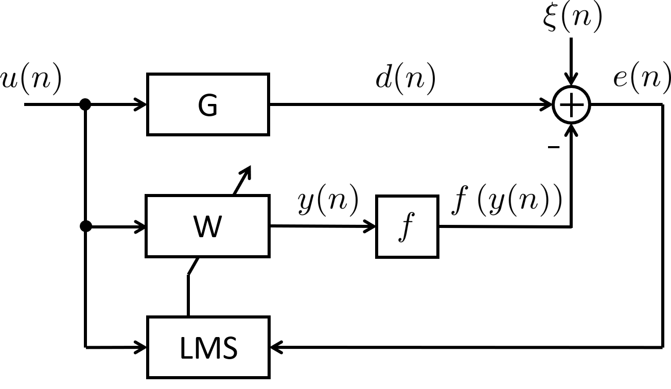
Figure 1: Block diagram of the adaptive system.

The adaptive filter W is an $N$-tap finite-duration impulse response (FIR) filter. Its coefficient vector is

$$\bm{w}(n) =[w_{1}(n),w_{2}(n),\ldots,w_{N}(n)]^{\top},$$ (2)

where $n$ denotes the time step. Although the dimension $M$ of $\bm{g}_{0}$ is generally unknown in advance, we assume that the tap length $N$ of the adaptive filter W is set to satisfy

$$N\geq M,$$ (3)

because it is straightforward to design an adaptive filter W of tap length $N$ with a margin. Also, let $\bm{g}$ be a vector made into $N$ dimensions by adding $N-M$ zeros to $\bm{g}_{0}$. That is,

$$\bm{g} =[g_{1},g_{2},\ldots,g_{M},g_{M+1},\ldots,g_{N}]^{\top},$$ (4)

$$g_{i} =0,\ \ i=M+1,\ldots,N.$$ (5)

Note that while it is assumed in most previous studies that the dimensions of $\bm{g}_{0}$ and $\bm{w}$ are the same [22, 23, 24, 27, 28, 29], our model essentially allows an arbitrary $\bm{g}_{0}$ and does not make strict assumptions on its dimension $M$ or its elements $\{g_{i}\},i=1,\ldots,M$.

We define the parameter $\sigma_{g}^{2}$ as

$$\sigma_{g}^{2} \triangleq\frac{1}{N}\|\bm{g}_{0}\|_{2}^{2}=\frac{1}{N}\|\bm{g}\|_{2}^{2}=\frac{1}{N}\sum_{i=1}^{N}g_{i}^{2}.$$ (6)

As will become clear later, our theory depends on the unknown system G only via $\sigma_{g}^{2}$. To demonstrate this, we will show in Sec. IV that the theory is valid for actual $\bm{g}_{0}$ obtained experimentally.

The input signal $u(n)$ is assumed to be independently drawn from a distribution with

$$\left\langle u(n)\right\rangle =0,\hskip 28.45274pt\left\langle u(n)^{2}\right\rangle=\sigma^{2}.$$ (7)

That is, the input signal is white. Although the assumption that the input signal is white may seem to be a major constraint in this analysis, the white input model is an important part of practical applications, especially in system identification, and provides a clear insight into the behavior of the algorithm. Moreover, the white input case provides a baseline for other cases[22]. The tap input vector ${\bm{u}}(n)$ at time step $n$ is

$$\bm{u}(n) =[u(n),u(n-1),\ldots,u(n-N+1)]^{\top}.$$ (8)

Note that only the mean and variance of the distribution are specified in (7). No specific distributions, for example, the Gaussian distribution, are assumed.

Outputs of the unknown system G and the adaptive filter W are convolutions of their own coefficients and a sequence of input signals. That is, the outputs $d(n)$ of G and $y(n)$ of W are respectively

$$d(n) =\bm{g}^{\top}\bm{u}(n)=\sum_{i=1}^{N}g_{i}u(n-i+1),$$ (9)

$$y(n) =\bm{w}(n)^{\top}\bm{u}(n)=\sum_{i=1}^{N}w_{i}(n)u(n-i+1).$$ (10)

The nonlinearity of the adaptive filter W is modeled by the function $f$ placed after W. The function $f$ represents the clipping saturation-type nonlinearity and is expressed as

$$f(x) =\begin{cases}S,&x>S\\ -S,&x<-S\\ x,&\mbox{otherwise}\end{cases},$$ (11)

where $S$ is a nonnegative real number. Figure 2 shows the function $f$.

Figure 2: Clipping saturation-type nonlinearity.

The error signal $e(n)$ is generated by adding an independent background noise $\xi(n)$ to the difference between $d(n)$ and $y(n)$. That is,

$$e(n) =d(n)-f(y(n))+\xi(n).$$ (12)

Here, the mean and variance of $\xi(n)$ are zero and $\sigma_{\xi}^{2}$, respectively. Note that only the mean and variance of the distribution are specified. No specific distributions, for example, the Gaussian distribution, are assumed for the background noise.

The LMS algorithm[32] is used to update the adaptive filter. That is,

$$\bm{w}(n+1) =\bm{w}(n)+\mu e(n)\bm{u}(n),$$ (13)

where $\mu$ is a positive real number and is called the step size.

III Analysis

In this section, we theoretically analyze the behaviors of the adaptive system with clipping saturation-type nonlinearity by the statistical-mechanical method. From (12), the MSE is expressed as

$$\left\langle e^{2}\right\rangle =\left\langle\left(d-f(y)+\xi\right)^{2}\right\rangle$$ (14)

$$=\left\langle d^{2}\right\rangle+\left\langle f(y)^{2}\right\rangle-2\left\langle df(y)\right\rangle+\sigma_{\xi}^{2}.$$ (15)

In this section, we omit the time step $n$ unless otherwise stated to avoid a rather cumbersome notation. We assume $N\to\infty$ while keeping both $\sigma_{g}^{2}$ and

$$\rho^{2} \triangleq N\sigma^{2}$$ (16)

constant, in accordance with the statistical-mechanical method[33].

The normalized LMS (NLMS) algorithm[1, 2] is a practically important variant of the LMS algorithm, whose update rule is

$$\bm{w}(n+1) =\bm{w}(n)+\frac{\tilde{\mu}}{\|\bm{u}(n)\|_{2}^{2}}e(n)\bm{u}(n),$$ (17)

where $\tilde{\mu}$ is the step size. Note that since $\|\bm{u}(n)\|^{2}_{2}=N\sigma^{2}=\rho^{2}$, the analysis in this paper is equivalent to the analysis of the NLMS algorithm with $\tilde{\mu}=\rho^{2}\mu$ as the step size for a stationary input signal $u(n)$.

Then, from the central limit theorem, both $d$ and $y$ are stochastic variables that obey the Gaussian distribution. Their means are zero, and their variance–covariance matrix is

$$\bm{\Sigma} \triangleq\left\langle\left[d-\left\langle d\right\rangle,y-\left\langle y\right\rangle\right]^{\top}\left[d-\left\langle d\right\rangle,y-\left\langle y\right\rangle\right]\right\rangle$$ (18)

$$=\rho^{2}\begin{pmatrix}\sigma_{g}^{2}&r\\ r&Q\end{pmatrix}.$$ (19)

Here, $Q$ and $r$ are macroscopic variables that are respectively defined as

$$Q \triangleq\frac{1}{N}\bm{w}^{\top}\bm{w},$$ (20)

$$r \triangleq\frac{1}{N}\bm{g}^{\top}\bm{w}.$$ (21)

The derivation of the means and variance–covariance matrix is given in detail in Appendix A.

We obtain three sample means in (15) as follows by carrying out the Gaussian integration for $d$ and $y$:

$$\left\langle d^{2}\right\rangle =\rho^{2}\sigma_{g}^{2},$$ (22)

$$\left\langle f(y)^{2}\right\rangle =S^{2}+\left(\rho^{2}Q-S^{2}\right)\mbox{erf}\left(\frac{S}{\sqrt{2\rho^{2}Q}}\right)$$

$$\hskip 11.38109pt-S\sqrt{\frac{2\rho^{2}Q}{\pi}}\exp\left(-\frac{S^{2}}{2\rho^{2}Q}\right),$$ (23)

$$\left\langle df(y)\right\rangle =\rho^{2}r\ \mbox{erf}\left(\frac{S}{\sqrt{2\rho^{2}Q}}\right),$$ (24)

where $\mbox{erf}(\cdot)$ is an error function defined as

$$\mbox{erf}(x) \triangleq\frac{2}{\sqrt{\pi}}\int_{0}^{x}\exp\left(-\tau^{2}\right)\mathrm{d}\tau.$$ (25)

Equation (22) is easily derived from (19). Equations (23) and (24) are derived in detail in Appendices B and C, respectively.

From (15), (22), (23), and (24), we obtain the MSE as

$$\left\langle e^{2}\right\rangle =\rho^{2}\sigma_{g}^{2}+S^{2}+\left(\rho^{2}Q-2\rho^{2}r-S^{2}\right)\mbox{erf}\left(\frac{S}{\sqrt{2\rho^{2}Q}}\right)$$

$$\hskip 11.38109pt-S\sqrt{\frac{2\rho^{2}Q}{\pi}}\exp\left(-\frac{S^{2}}{2\rho^{2}Q}\right)+\sigma_{\xi}^{2}.$$ (26)

This formula shows that the MSE is a function of the macroscopic variables $Q$ and $r$. Therefore, we derive differential equations that describe the dynamical behaviors of these variables in the following. Multiplying both sides of (13) on the left by $\bm{g}^{\top}$ and using (21), we obtain

$$Nr(n+1) =Nr(n)+\mu e(n)d(n).$$ (27)

We introduce time $t$ defined by

$$t \triangleq n/N,$$ (28)

and use it to represent the adaptive process. Then, $t$ becomes a continuous variable since the limit $N\rightarrow\infty$ is considered. These calculations are in line with the statistical-mechanical analysis of online learning[38].

If the adaptive filter is updated $N\mathrm{d}t$ times in an infinitely small time $\mathrm{d}t$, we can obtain $N\mathrm{d}t$ equations as

$$Nr(n+1) =Nr(n)+\mu e(n)d(n),$$ (29)

$$Nr(n+2) =Nr(n+1)+\mu e(n+1)d(n+1),$$ (30)

$$\vdots\ \ \ \ \ \hskip 4.2679pt\vdots\ \ \ \ \ \ \ \vdots$$

$$Nr(n+N\mathrm{d}t) =Nr(n+N\mathrm{d}t-1)$$

$$\hskip 14.22636pt+\mu e(n+N\mathrm{d}t-1)d(n+N\mathrm{d}t-1).$$ (31)

Summing all these equations, we obtain

$$Nr(n+N\mathrm{d}t) =Nr(n)+\mu\sum_{n^{\prime}=n}^{n+N\mathrm{d}t-1}e(n^{\prime})d(n^{\prime}).$$ (32)

Therefore, we obtain

$$N(r+\mathrm{d}r) =Nr+N\mathrm{d}t\mu\left\langle ed\right\rangle.$$ (33)

Here, from the law of large numbers, we have represented the effect of the probabilistic variables by their means since the updates are executed $N\mathrm{d}t$ times, that is, many times, to change $r$ by $\mathrm{d}r$. This property is called self-averaging in statistical mechanics[33]. From (12) and (33), we obtain a differential equation that describes the dynamical behavior of $r$ in a deterministic form as follows:

$$\frac{\mathrm{d}r}{\mathrm{d}t} =\mu\Bigl{(}\left\langle d^{2}\right\rangle-\left\langle df(y)\right\rangle\Bigr{)}.$$ (34)

Next, squaring both sides of (13) and proceeding in the same manner as for the derivation of the above differential equation for $r$, we can derive a differential equation for $Q$, which is given by

$$\frac{\mathrm{d}Q}{\mathrm{d}t} =\mu^{2}\rho^{2}\Bigl{(}\left\langle d^{2}\right\rangle-2\left\langle df(y)\right\rangle+\left\langle f(y)^{2}\right\rangle+\sigma_{\xi}^{2}\Bigr{)}$$

$$\hskip 11.38109pt+2\mu\Bigl{(}\left\langle dy\right\rangle-\left\langle yf(y)\right\rangle\Bigr{)}.$$ (35)

Here, we used the fact that in the limit of $N\rightarrow\infty$, $\mathbf{u}^{\top}\mathbf{u}=\|\mathbf{u}\|_{2}^{2}=\sum_{i=1}^{N}u(n-i+1)^{2}$ is no longer a random variable but a constant $\rho^{2}=N\sigma^{2}$ from the law of large numbers, so this can be taken out of the expectation operation $\langle\cdot\rangle$. This is precisely one of the strengths of the statistical-mechanical method, which assumes $N\rightarrow\infty$.

Equations (34) and (35) include five sample means. However, because three of the five means are already given in (22)–(24), we obtain the two remaining means as follows by carrying out the Gaussian integration for $d$ and $y$:

$$\left\langle dy\right\rangle =\rho^{2}r,$$ (36)

$$\left\langle yf(y)\right\rangle =\rho^{2}Q\ \mbox{erf}\left(\frac{S}{\sqrt{2\rho^{2}Q}}\right).$$ (37)

Equation (36) is easily derived from (19). Equation (37) is derived in detail in Appendix D.

Substituting (22)–(24), (36), and (37) into (34) and (35), we obtain the concrete formulas of the simultaneous differential equations as follows:

$$\frac{\mathrm{d}r}{\mathrm{d}t} =\mu\rho^{2}\left(\sigma_{g}^{2}-r\ \mbox{erf}\left(\frac{S}{\sqrt{2\rho^{2}Q}}\right)\right),$$ (38)

$$\frac{\mathrm{d}Q}{\mathrm{d}t} =\mu\rho^{2}\Bigl{(}\mu\left(\rho^{2}Q-2\rho^{2}r-S^{2}\right)-2Q\Bigr{)}\mbox{erf}\left(\frac{S}{\sqrt{2\rho^{2}Q}}\right)$$

$$\hskip 11.38109pt-\mu^{2}\rho^{2}S\sqrt{\frac{2\rho^{2}Q}{\pi}}\exp\left(-\frac{S^{2}}{2\rho^{2}Q}\right)$$

$$\hskip 11.38109pt+\mu\rho^{2}\left(\mu\left(\rho^{2}\sigma_{g}^{2}+S^{2}+\sigma_{\xi}^{2}\right)+2r\right).$$ (39)

We numerically solve the derived simultaneous differential equations, since they cannot be analytically solved. Substituting the obtained numerical solution into (26), we obtain the MSE learning curves.

From (6), (20), and (21), we can also obtain the MSD, or misalignment, as a function of the macroscopic variables $Q$ and $r$ as follows:

MSD $$=\|\bm{g}-\bm{w}\|_{2}^{2}$$ (40)

$$=\|\bm{g}\|_{2}^{2}-2\bm{g}^{\top}\bm{w}+\|\bm{w}\|_{2}^{2}$$ (41)

$$=N(\sigma_{g}^{2}-2r+Q).$$ (42)

Equation (42) shows that the MSD is proportional to the tap length $N$ in the model setting in this paper; therefore, we normalize the MSD by $N$ and call it the normalized MSD.

IV Results and Discussion

IV-A Learning curves

We first investigate the validity of the theory by comparing theoretical results with simulation results with regard to the dynamical behaviors of the MSE and normalized MSD, that is, the learning curves. Figures 3 and 4 show the learning curves obtained using the theory derived in the previous section, along with the corresponding simulation results. In these figures, the curves represent theoretical results and the polygonal lines represent simulation results. In the theoretical calculation and simulations throughout this section, $\rho^{2}=\sigma_{g}^{2}=1$. In the theoretical calculation, the results are obtained by substituting $r$ and $Q$, which are respectively obtained by solving (38) and (39), into (26) and (42). Here, (38) and (39) are numerically solved by the Runge–Kutta method. In the computer simulations, the number of taps of the adaptive filter W is $N=400$ and ensemble means for 1000 trials are plotted. The impulse response $\bm{g}_{0}$ of the unknown system G in all computer simulations in this paper is obtained experimentally by measurement[39] and is shown in Fig. 5. Its dimension $M$ is 256. Note that $\bm{g}_{0}$ has been normalized to satisfy (6). All initial values $w_{i}(0),\ i=1,\ldots,N$ of the coefficients are set to zero in the simulation, and the initial condition $r(0)=Q(0)=0$ is used in the theoretical calculation. Figures 3 and 4 show that the theory derived in this paper predicts the simulation results well in terms of average values.

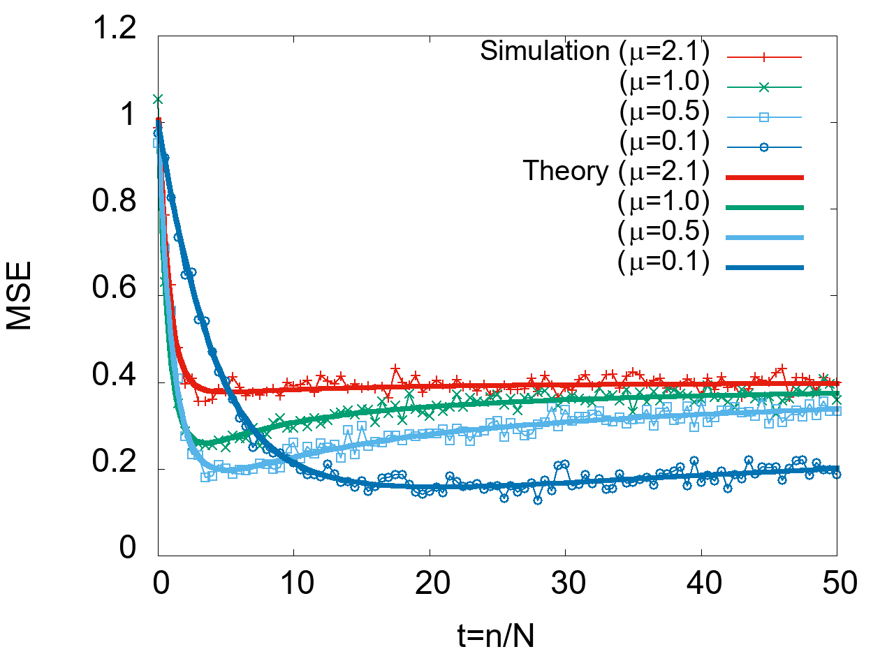
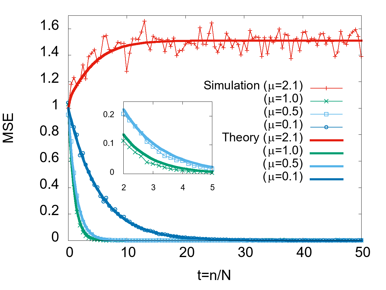
(a) $S=1,\sigma_{\xi}^{2}=0$

(b) $S=3,\sigma_{\xi}^{2}=0$

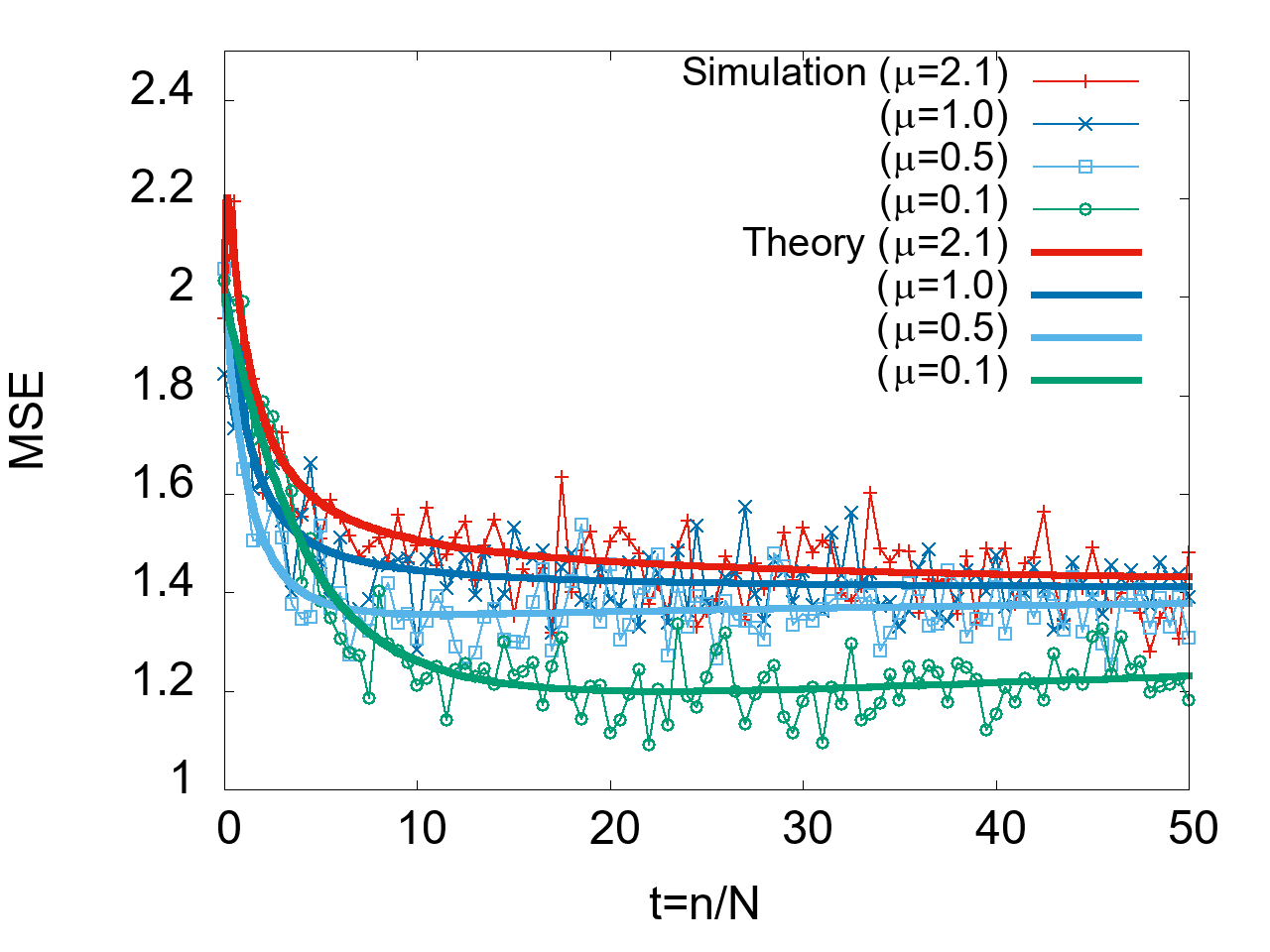
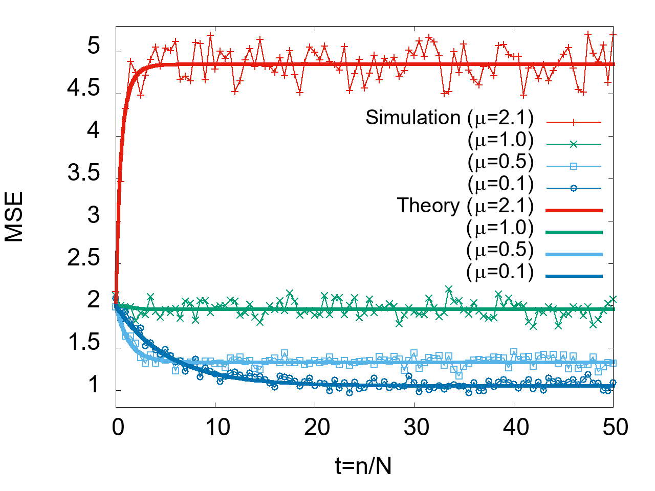
(c) $S=1,\sigma_{\xi}^{2}=1$

(d) $S=3,\sigma_{\xi}^{2}=1$

Figure 3: MSE learning curves.

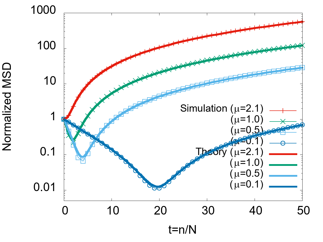
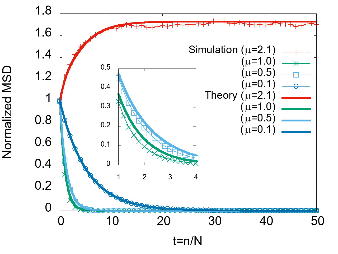
(a) $S=1,\sigma_{\xi}^{2}=0$

(b) $S=3,\sigma_{\xi}^{2}=0$

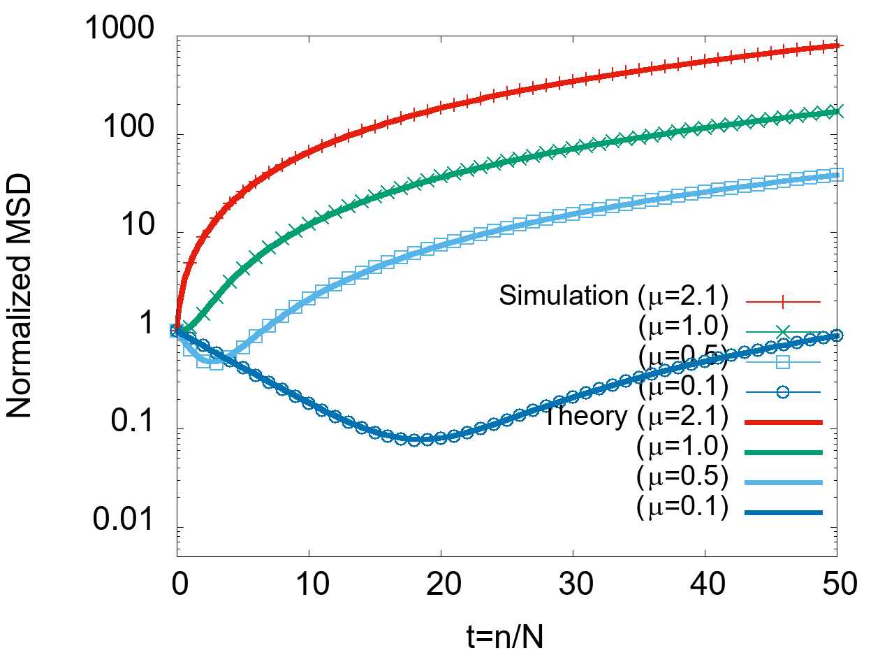
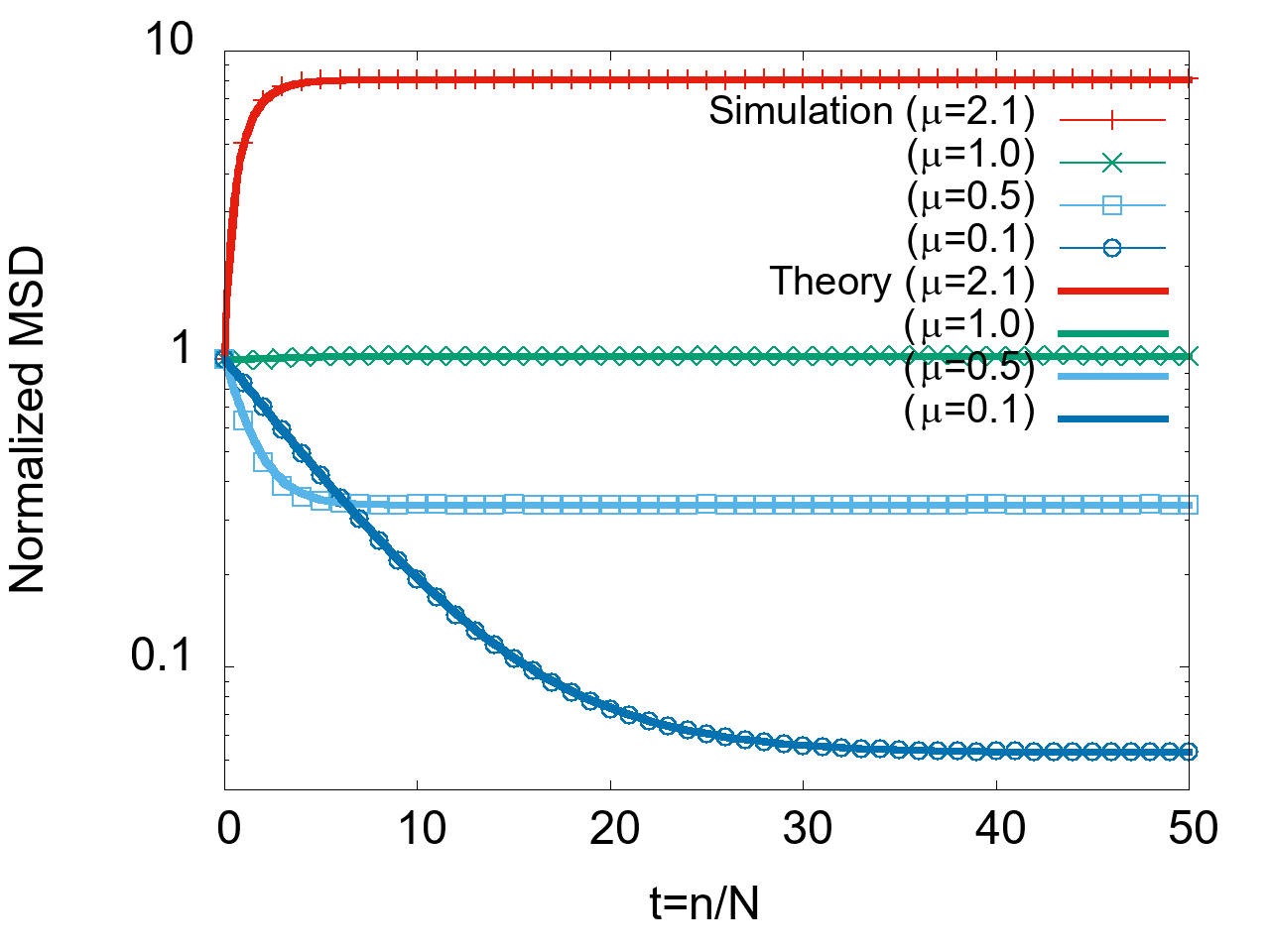
(c) $S=1,\sigma_{\xi}^{2}=1$

(d) $S=3,\sigma_{\xi}^{2}=1$

Figure 4: Normalized MSD learning curves.

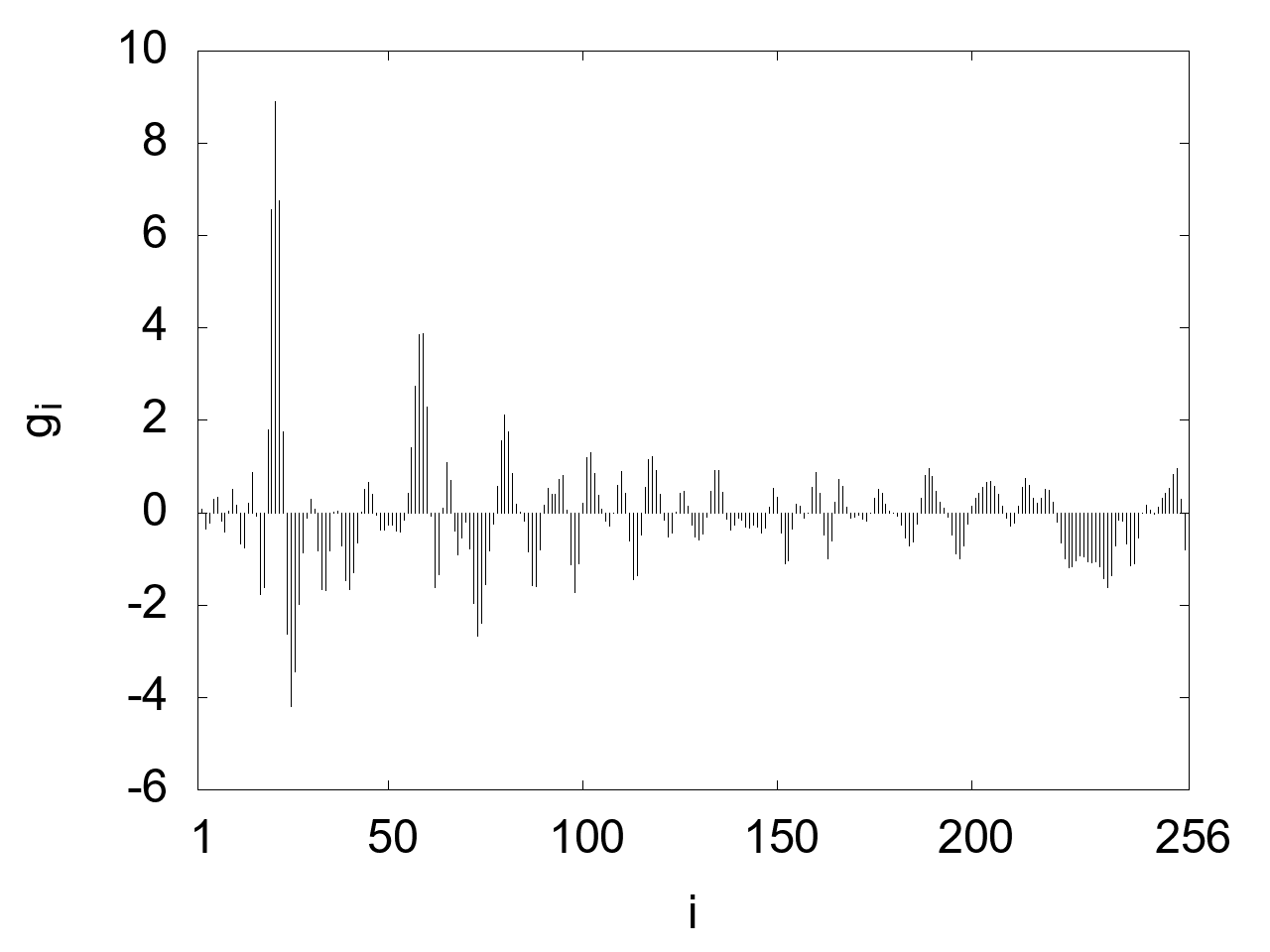
Figure 5: Impulse response $\bm{g}_{0}$ of the unknown system G used in all computer simulations in this paper.

Since statistical-mechanical analysis assumes $N\rightarrow\infty$, it is important to investigate how well the theory explains the simulation results with small $N$. Figure 6 shows the theoretical learning curves along with the simulation results for $N=400,100,20$, and $5$. In the computer simulations, the unknown system coefficient vectors are generated by uniformly sampling the impulse responses shown in Fig. 5 and normalizing them to satisfy (6). Figure 6 shows that, especially when $S$ and $\mu$ are large, there is significant disagreement between the simulation results with small $N$ and the theoretical results. The reason for this disagreement is considered to be that the theory is derived using the long-filter assumption, that is, $N\rightarrow\infty$, whereas the simulations are executed using finite values of $N$. The dependence of the disagreement on $N$ is an example of the phenomenon known as the finite-size effect in statistical mechanics. Note, however, that when $S$ or $\mu$ is small, the theory is in good agreement with the simulation, even if $N=20$ or 5.

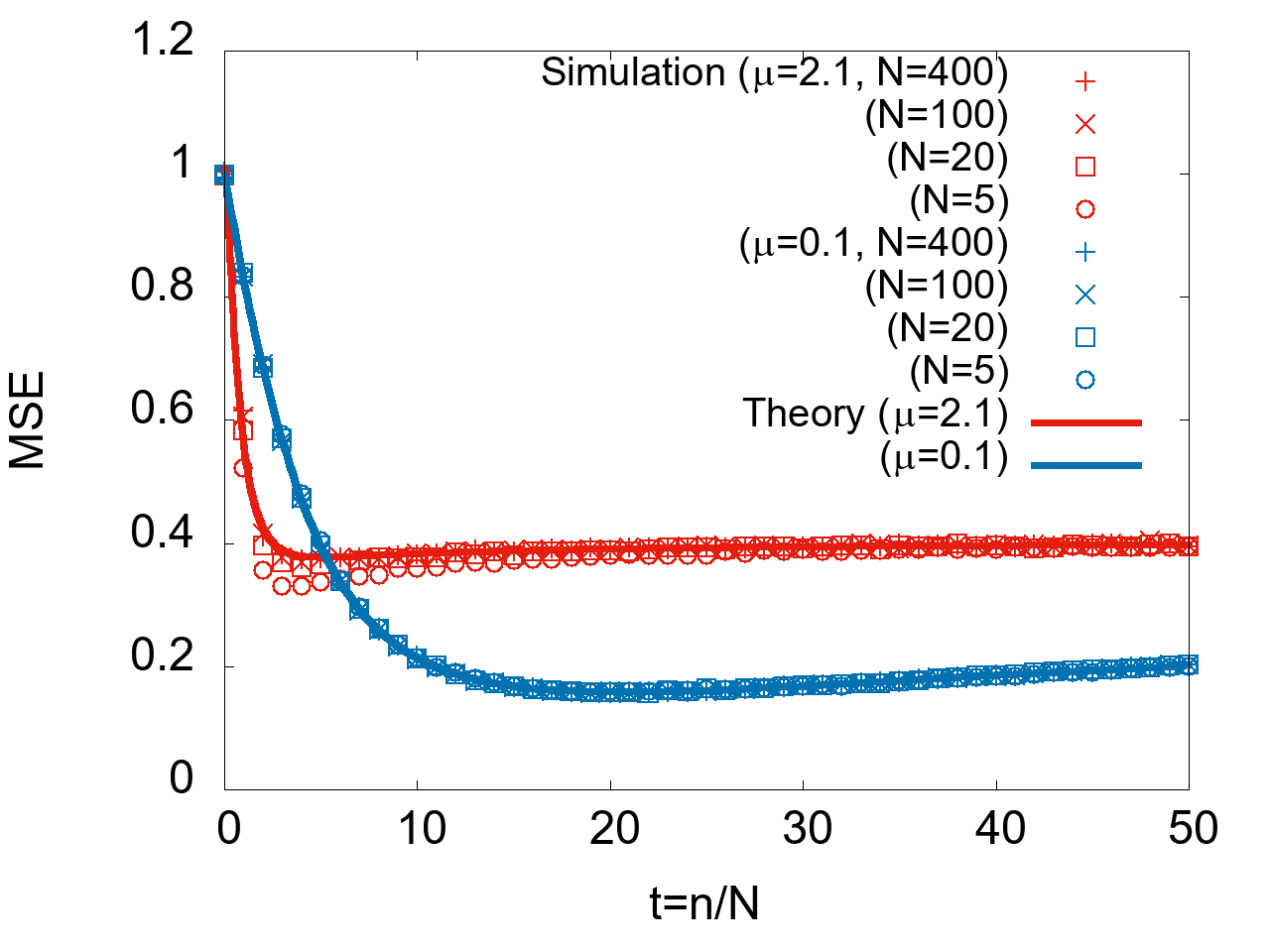
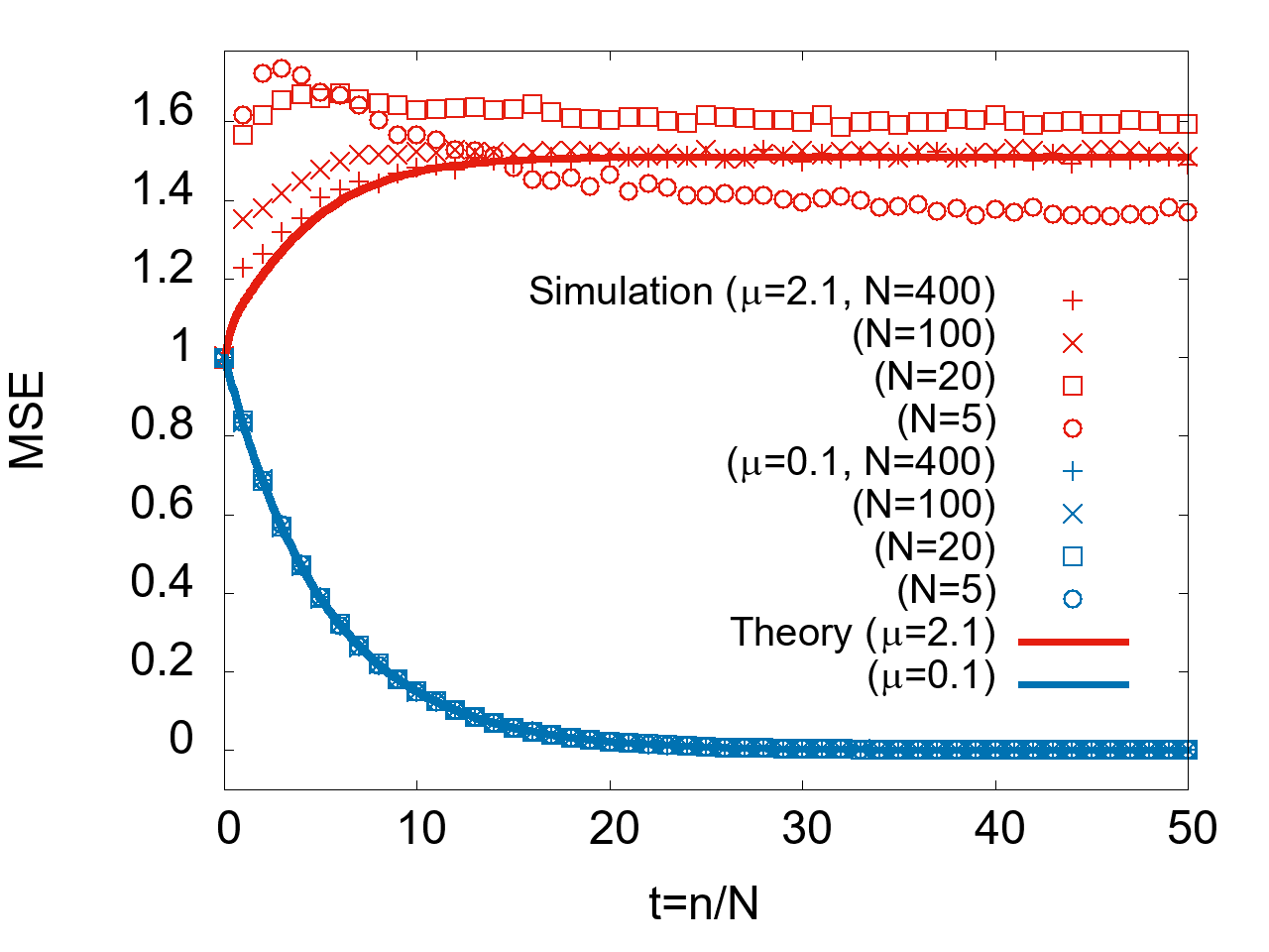
(a) $S=1,\sigma_{\xi}^{2}=0$

(b) $S=3,\sigma_{\xi}^{2}=0$

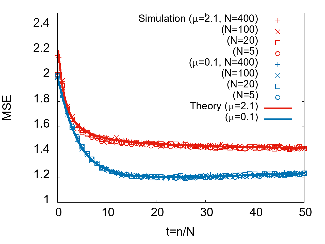
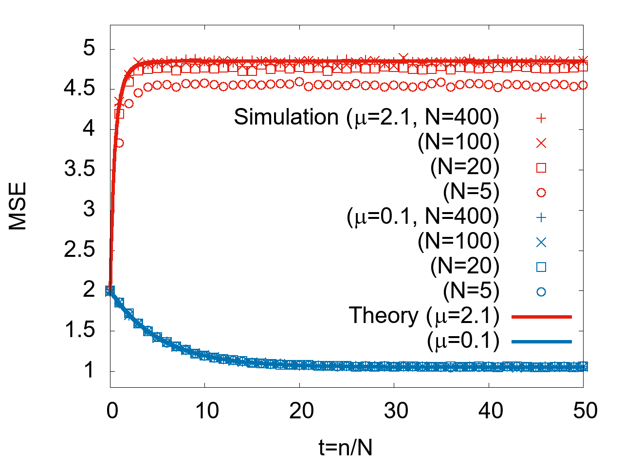
(c) $S=1,\sigma_{\xi}^{2}=1$

(d) $S=3,\sigma_{\xi}^{2}=1$

Figure 6: MSE learning curves obtained by simulations with small $N$ and theory.

Figure 7 shows examples of the MSE learning curves when the initial values $w_{i}(0),\ i=1,\ldots,N$ of the filter coefficients are not zero. In the computer simulation, the initial values of the filter coefficients are independently drawn from a Gaussian distribution with a mean 0 and a variance 1. In response to this, the initial conditions $r(0)=0$ and $Q(0)=1$ are used in the theoretical calculation. Figures 7–7 show that the theory derived in this paper predicts the simulation results well even if the initial values of the filter coefficients are not zero. Comparing these figures with Figs. 3–3, it can be seen that the initial values of the MSE are increased by the non-zero initial values of the filter coefficients. On the other hand, their steady-state values remain the same. Hereafter, the initial values of the filter coefficients are assumed to be zero.

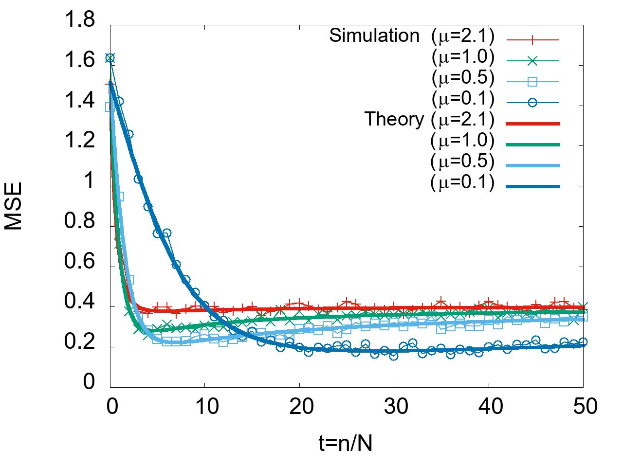
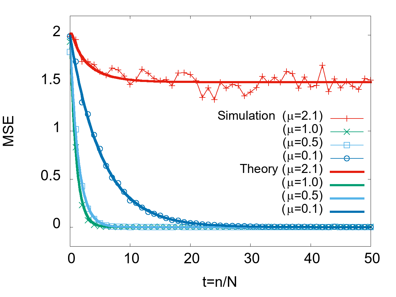
(a) $S=1,\sigma_{\xi}^{2}=0$

(b) $S=3,\sigma_{\xi}^{2}=0$

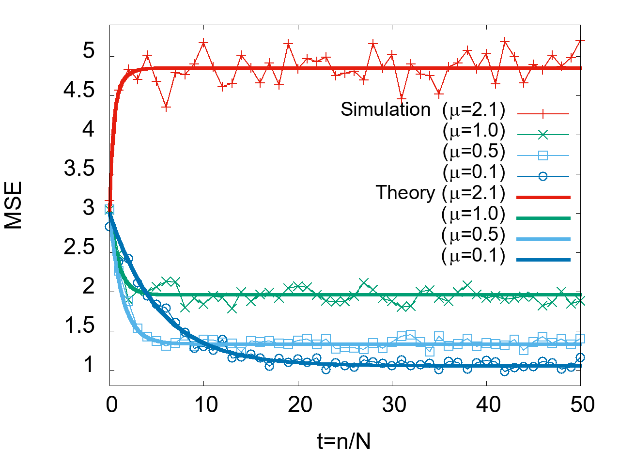
(c) $S=1,\sigma_{\xi}^{2}=1$

(d) $S=3,\sigma_{\xi}^{2}=1$

Figure 7: MSE learning curves when the initial values of the filter coefficients are not zero.

From Figs. 3–3, it seems that the MSE almost converges at $t=50$ regardless of the step size $\mu$ for both $S=1$ and 3. However, Figs. 4 and 4 show that the normalized MSD continues to increase for $S=1$. Next, we show the MSE at $t=10,100$, and $1000$ in Figs. 8 and 9 to investigate the relationship between the saturation value $S$ and the MSE. For the computer simulations, the medians and standard deviations in 100 trials are plotted using error bars. Figures 8 and 9 show that the MSE increases when $S$ is in the range of 1.1–1.3, and this tendency becomes increasingly pronounced with time.

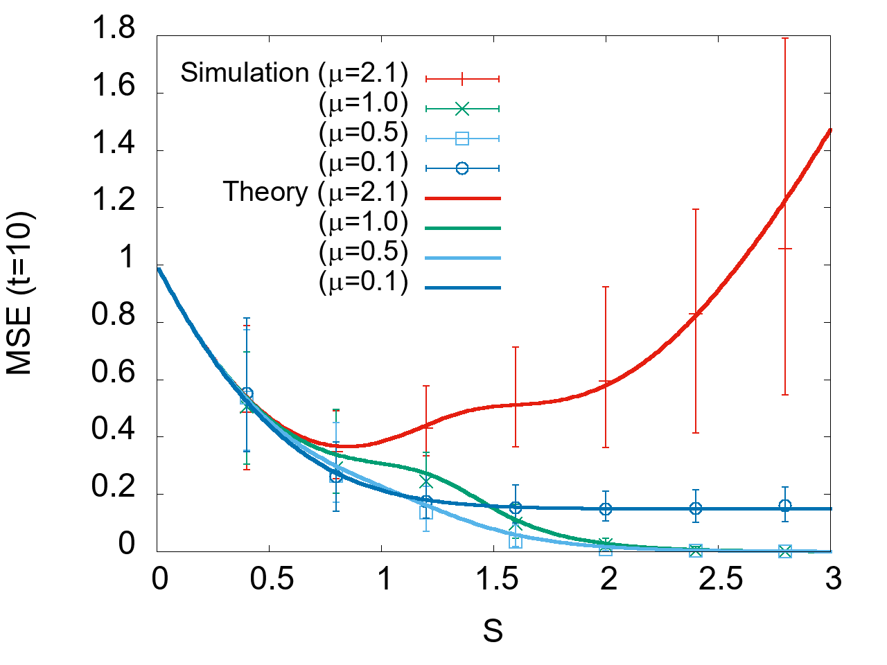
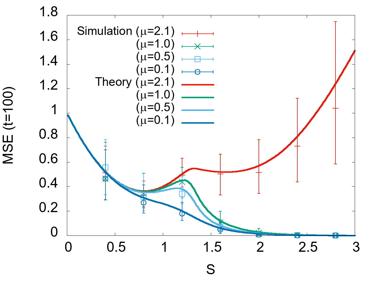
(a) $t=10$

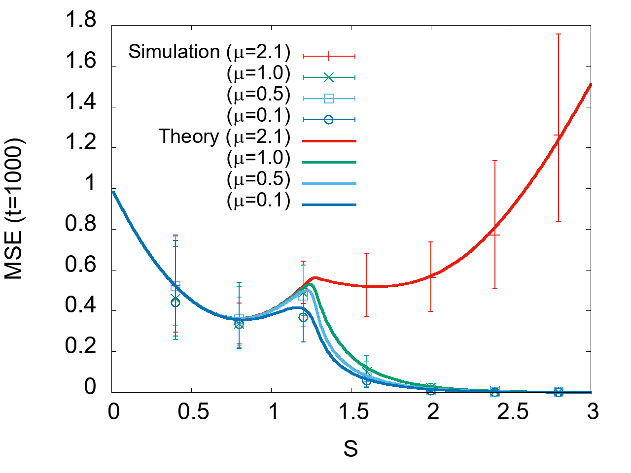
(b) $t=100$

(c) $t=1000$

Figure 8: MSE at $t=10,100$, and $1000$ ($\sigma_{\xi}^{2}=0$).

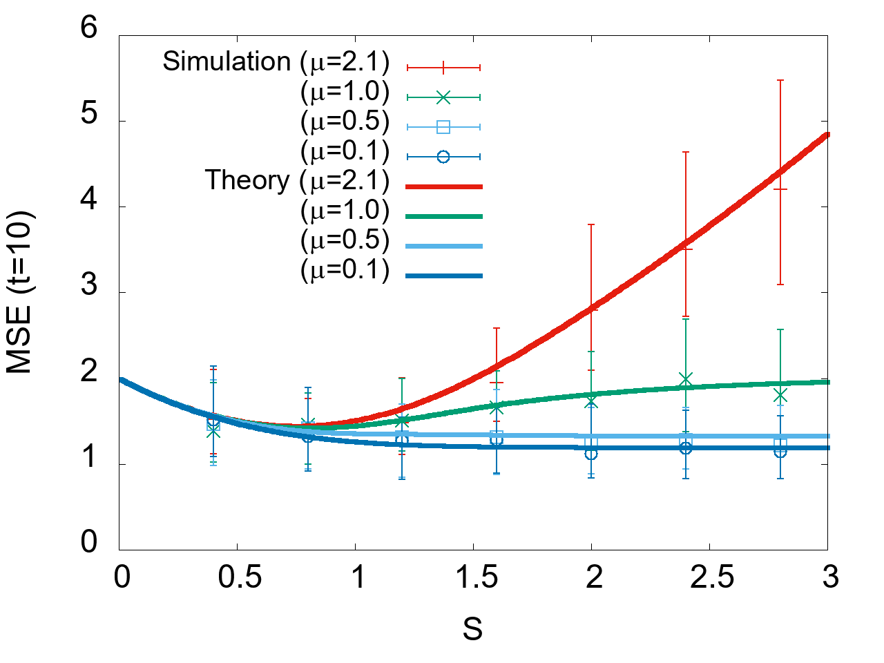
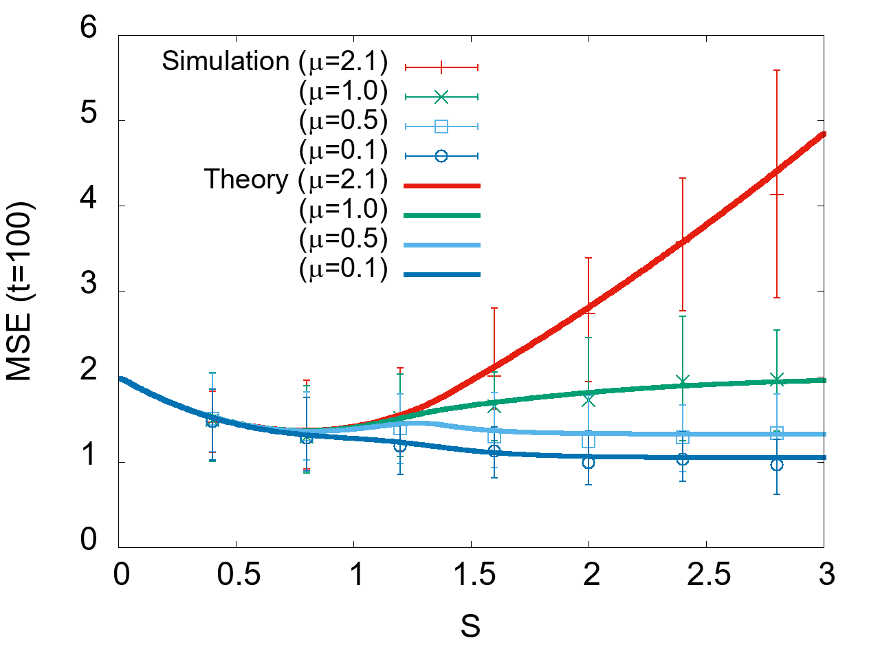
(a) $t=10$

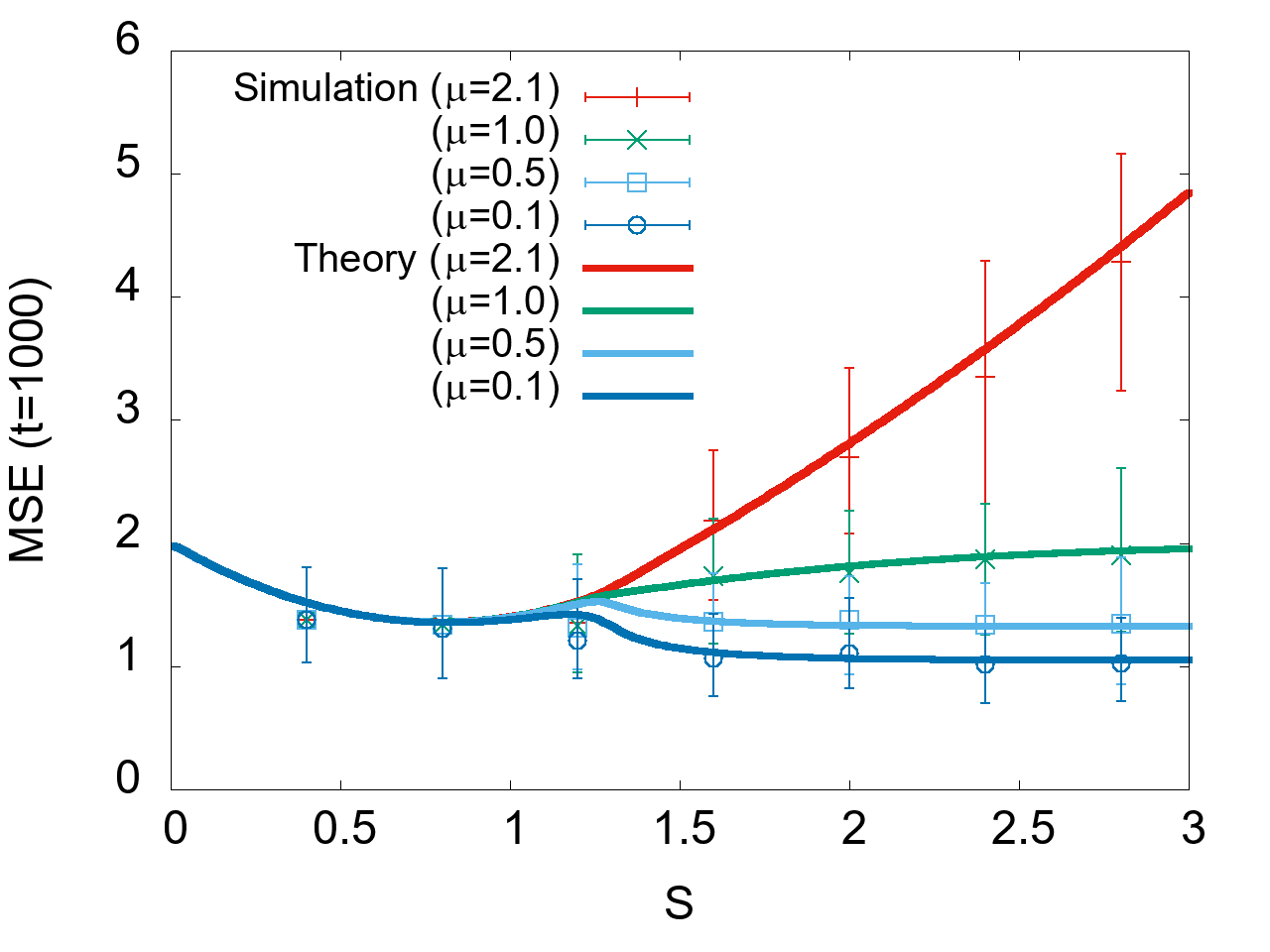
(b) $t=100$

(c) $t=1000$

Figure 9: MSE at $t=10,100$, and $1000$ ($\sigma_{\xi}^{2}=1$).

IV-B Critical value $S_{C}$ and steady-state analysis when $S>S_{C}$

To clarify the phenomenon of increasing MSE described in the previous subsection, we investigate the steady-state values of the macroscopic variables $r,Q$, and MSE. If steady-state values of $r$ and $Q$ exist, they can be obtained by numerically solving the simultaneous equations that are obtained by substituting zeros into the left-hand sides of the simultaneous differential equations (38) and (39). Figure 10 shows the numerically obtained results for $Q$ along with the corresponding simulation results at $t=10^{4}$. This value of $t$ in the simulation is sufficient for $Q$ to reach a steady-state value. When the saturation value $S$ is larger than $S_{C}=1.25331\cdots$, a numerical solution is found. However, when $S$ is smaller than $S_{C}$, no numerical solution is found. Of course, no numerical solution found for the simultaneous equations is only a necessary condition for $r$ and $Q$ to diverge, not a sufficient condition. In other words, no numerical solution found does not necessarily indicate that $r$ or $Q$ diverges. Of course, it is most desirable to prove mathematically that $r$ and/or $Q$ diverge, but this is difficult because of the complexity of the simultaneous differential equations (38) and (39). Therefore, we investigate the dynamical behavior of $Q$ for $S<S_{C}$ by means of theoretical numerical calculations and computer simulations. Figures 11 and 11 show the results. In these figures, $Q$ increases monotonically in all cases. These results strongly indicate that $Q$ diverges regardless of the step size and the presence of background noise when $S<S_{C}$. Since $Q$ is proportional to the square of the $\ell_{2}$-norm of $\bm{w}$, as seen from (20), the divergence of $Q$ means the divergence of the coefficient vector $\bm{w}$ of the adaptive filter W. When $S>S_{C}$, we can obtain the steady-state MSE by substituting the steady-state values of $r$ and $Q$ into (26). Note that it is clarified in Sec. IV-D that the exact value of $S_{C}=1.25331\cdots$ is $\sqrt{\frac{\pi}{2}}$.

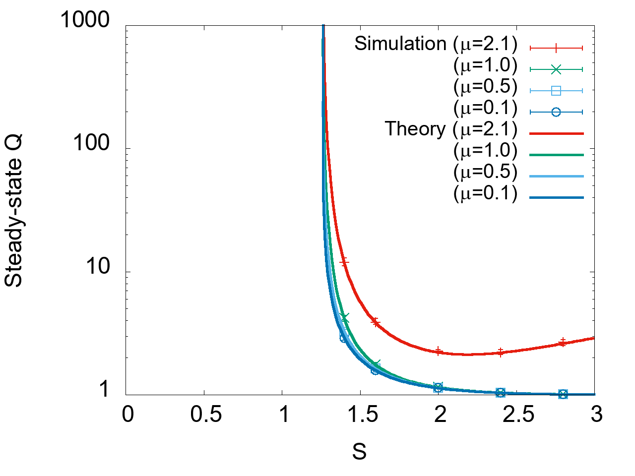
(a) $\sigma_{\xi}^{2}=0$

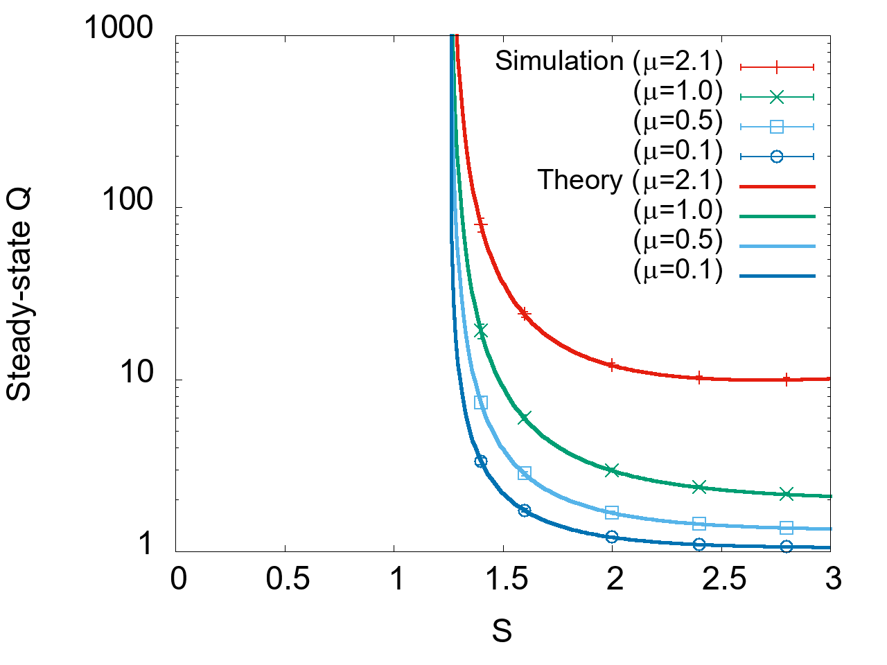
(b) $\sigma_{\xi}^{2}=1$

Figure 10: Steady-state $Q$.

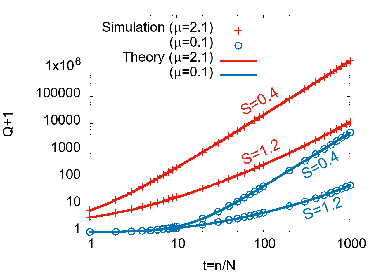
(a) $\sigma_{\xi}^{2}=0$

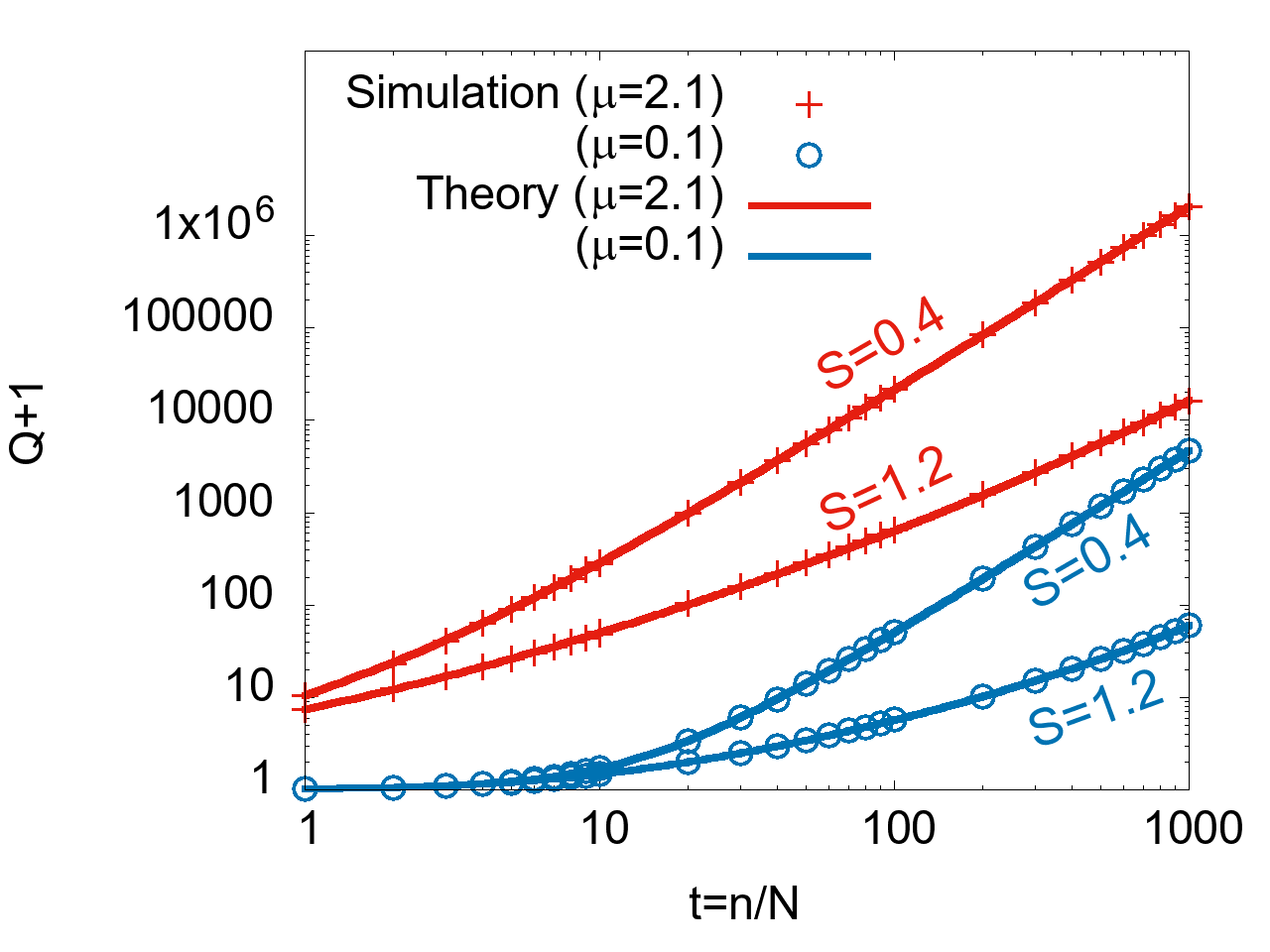
(b) $\sigma_{\xi}^{2}=1$

Figure 11: Dynamical behaviors of $Q$ when $S<S_{C}$.

IV-C Asymptotic analysis when $S<S_{C}$

On the basis of the results obtained in the previous subsection, we henceforth assume that $Q$ diverges in the limit $t\rightarrow\infty$ when $S<S_{C}$. However, Figs. 8 and 9 show that the MSE appears to converge even when $S<S_{C}$. Therefore, an asymptotic analysis of the behavior of the system when $S<S_{C}$ is given in this subsection. From (6), (20), and (21), we obtain

$$r =\sigma_{g}\sqrt{Q}\cos\theta.$$ (43)

Here, $\theta$ is the angle between vectors $\bm{g}$ and $\bm{w}$. From (38), (39), and (43), we obtain

$$\cos\theta \xrightarrow{t\rightarrow\infty}1.$$ (44)

Equation (44) is derived in detail in Appendix E, where the approximations

$$\mbox{erf}\left(x\right) =\frac{2}{\sqrt{\pi}}\sum_{n=0}^{\infty}\frac{(-1)^{n}x^{2n+1}}{n!(2n+1)}\simeq\frac{2}{\sqrt{\pi}}x (|x|\ll 1),$$ (45)

$$\exp\left(x\right) =\sum_{n=0}^{\infty}\frac{x^{n}}{n!}\simeq 1+x (|x|\ll 1)$$ (46)

are used.

Equation (44) means that the directions of $\bm{g}$ and $\bm{w}$ coincide even when $S<S_{C}$, although $\bm{w}$ diverges as described in Sec. IV-B. Note that this property does not depend on $\mu,\rho^{2},\sigma_{g}^{2}$, or $\sigma_{\xi}^{2}$.

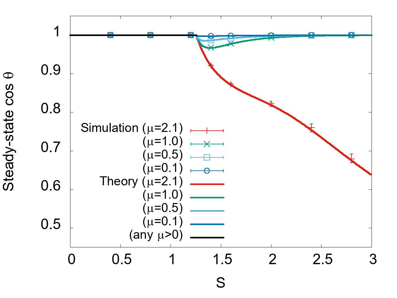
(a) $\sigma_{\xi}^{2}=0$

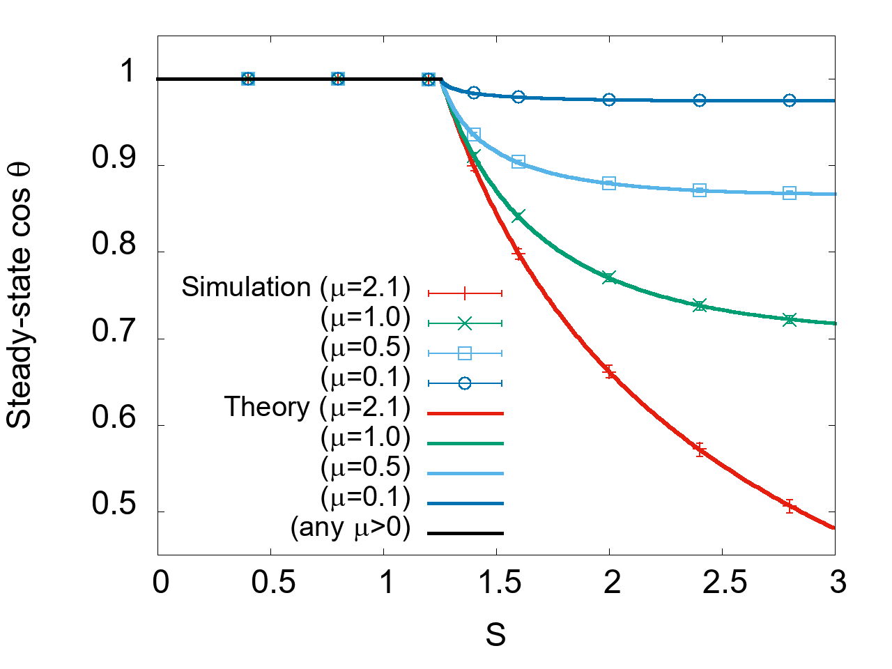
(b) $\sigma_{\xi}^{2}=1$

Figure 12: Steady-state $\cos\theta=r/(\sigma_{g}\sqrt{Q})$.

As described so far, $Q$ diverges and $\cos\theta=1$ in the limit $t\rightarrow\infty$ when $S<S_{C}$. Then, the MSE is

$$\left\langle e^{2}\right\rangle =S^{2}-2\sigma_{g}\rho\sqrt{\frac{2}{\pi}}S+\sigma_{g}^{2}\rho^{2}+\sigma_{\xi}^{2}.$$ (47)

Equation (47) is derived in detail in Appendix F. Although $\bm{w}$ diverges when $S<S_{C}$, (47) shows that the MSE converges. The converged value does not depend on the step size $\mu$, and it is a quadratic function of $S$. The converged value is minimum, $\sigma_{g}^{2}\rho^{2}\left(1-\frac{2}{\pi}\right)+\sigma_{\xi}^{2}$, when $S=\sigma_{g}\rho\sqrt{\frac{2}{\pi}}$. Figure 12 shows the theoretically obtained steady-state values of $\cos\theta=r/(\sigma_{g}\sqrt{Q})$, along with the corresponding simulation results at $t=10^{4}$. This value of $t$ in the simulation is sufficient for $\cos\theta$ to reach a steady-state value. In this figure, for $S>S_{C}$, theoretically obtained values calculated using the steady-state values of $r$ and $Q$ given in Sec. IV-B are plotted. On the other hand, for $S<S_{C}$, the theoretically obtained value obtained using (44) is plotted.

Figure 13 shows the theoretically obtained steady-state values of the MSE, along with the corresponding simulation results at $t=10^{4}$. This value of $t$ in the simulation is sufficient for the MSE to reach a steady-state value. In this figure, for $S>S_{C}$, the theoretically obtained results of the steady-state analysis described in Sec. IV-B are plotted. On the other hand, for $S<S_{C}$, the theoretical result obtained using (47) is plotted. As Fig. 13 and (47) show, for $S<S_{C}$, the steady-state MSE is independent of the step size $\mu$. On the other hand, for $S>S_{C}$, the steady-state MSE depends on $\mu$, but the MSE never diverges because $|f((y(n))|\leq S$. From the above, there is no upper bound on $\mu$ for the MSE to converge.

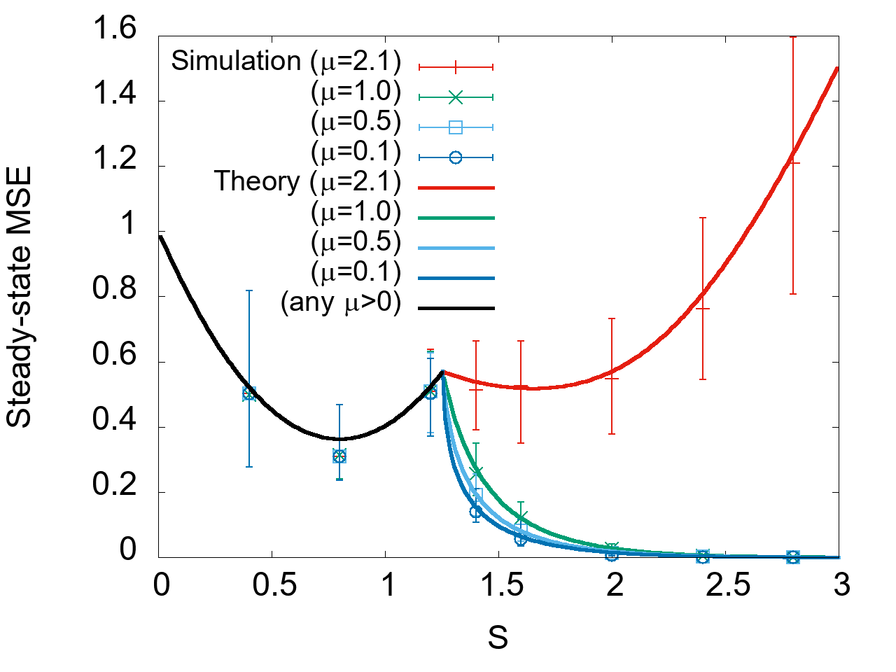
(a) $\sigma_{\xi}^{2}=0$

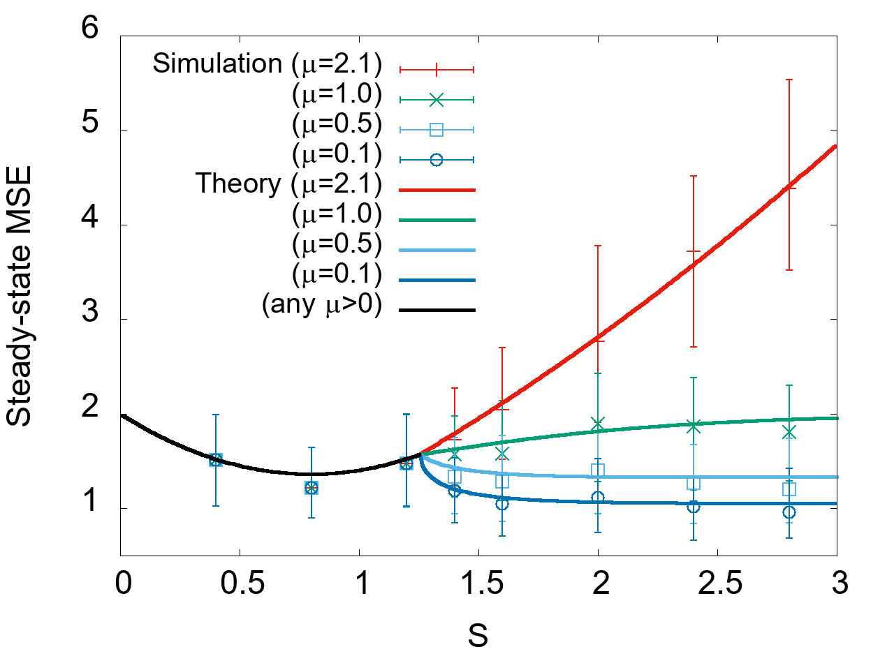
(b) $\sigma_{\xi}^{2}=1$

Figure 13: Steady-state MSE.

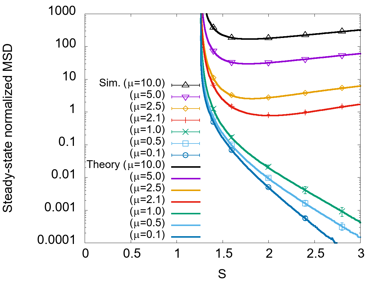
(a) $\sigma_{\xi}^{2}=0$

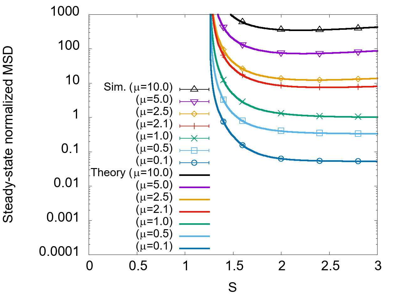
(b) $\sigma_{\xi}^{2}=1$

Figure 14: Steady-state normalized MSD.

Figure 14 shows the theoretically obtained steady-state normalized MSD, along with the corresponding simulation results at $t=10^{4}$. This value of $t$ in the simulation is sufficient for the normalized MSD to reach a steady-state value. This figure shows that the normalized MSD diverges because $Q$ diverges in the limit $S\downarrow S_{C}$, where $S\downarrow S_{C}$ denotes that $S$ decreases in value approaching $S_{C}$. That is, the condition in which the adaptive system is mean-square stable[2] is $S>S_{C}$. Although not mathematically proven, Fig. 14 suggests that for $S>S_{C}$, the normalized MSD converges regardless of the step size $\mu$.

IV-D Exact derivation of the critical value $S_{C}$

As described so far, the properties of the adaptive system switch markedly at $S=S_{C}$. That is, when $S>S_{C}$, the MSE and normalized MSD converge. In other words, the adaptive system is mean-square stable. The converged values depend on the step size $\mu$. On the other hand, when $S<S_{C}$, the normalized MSD diverges and the MSE converges to a value that does not depend on $\mu$. In addition, the angle between the coefficient vector $\bm{g}$ of the unknown system G and the coefficient vector $\bm{w}$ of the adaptive filter W converges to zero.

In this subsection, we analytically obtain the critical value $S_{C}$. As described in Sec. IV-B,

$$\lim_{S\downarrow S_{C}}\lim_{t\rightarrow\infty}\frac{\mathrm{d}r}{\mathrm{d}t}=\lim_{S\downarrow S_{C}}\lim_{t\rightarrow\infty}\frac{\mathrm{d}Q}{\mathrm{d}t} =0.$$ (48)

As described in Secs. IV-B and IV-C,

$$\lim_{S\downarrow S_{C}}\lim_{t\rightarrow\infty}Q =\infty,$$ (49)

$$\lim_{S\downarrow S_{C}}\lim_{t\rightarrow\infty}\cos\theta =1.$$ (50)

Substituting (45), (46), and (48)–(50) into (38) and (39) and solving for $S_{C}$, we obtain

$$S_{C} =\sigma_{g}\rho\sqrt{\frac{\pi}{2}}.$$ (51)

Equation (51) shows that the critical value $S_{C}$ is proportional to $\sigma_{g}$ and $\rho$ defined by (6) and (16), respectively. In addition, we see that the critical value of $S_{C}=1.25331\cdots$ numerically obtained in Sec. IV-B is, in fact, $\sqrt{\frac{\pi}{2}}$.

V Conclusions

We analyzed the behaviors of an adaptive system in which the output of the adaptive filter has the clipping saturation-type nonlinearity by the statistical-mechanical method. As a result, it was clarified that the saturation value $S$ has a critical value $S_{C}$ at which the system’s mean-square stability and instability switch. Finally, $S_{C}$ was exactly derived by asymptotic analysis. Although the theory by Costa et al.[22] and the theory proposed in this study take completely different approaches in terms of assumptions and methods, they both reveal the existence of critical values for nonlinearity, which is extremely interesting. That is, $\eta^{2}=1$ is the condition for establishing the “power threshold” in [22], and $S=S_{C}=\sigma_{g}\rho\sqrt{\frac{\pi}{2}}$ is the critical condition in our theory. However, our theory is valid for arbitrary step sizes, whereas Costa et al.[22] assume small step sizes. Our theory also well explains the simulation results in the case of strong nonlinearity $S<\sigma_{g}\rho\sqrt{\frac{\pi}{2}}$, which corresponds to $\eta^{2}>1$ in [22]. The findings in this study are non-trivial, albeit with respect to classical and simple models, and are significant both theoretically and practically.

Interesting theoretical problems that should be studied further remain. Analyses of other types of nonlinearities should be performed. For example, a dead-zone-type nonlinearity expressed by a piecewise linearity can be analyzed by the method described in this paper. In addition, the nonlinearities of other components should be analyzed in future studies.

Appendix A Derivation of means and variance–covariance matrix of $d$ and $y$

From (6), (7), (9), (10), (16), (20), and (21), we obtain the means, variances, and covariance of $d$ and $y$ as follows:

$$\left\langle d\right\rangle =\left\langle\sum_{i=1}^{N}g_{i}u(n-i+1)\right\rangle=\sum_{i=1}^{N}g_{i}\left\langle u(n-i+1)\right\rangle=0,$$ (52)

$$\left\langle y\right\rangle =\left\langle\sum_{i=1}^{N}w_{i}u(n-i+1)\right\rangle=\sum_{i=1}^{N}w_{i}\left\langle u(n-i+1)\right\rangle=0,$$ (53)

$$\left\langle d^{2}\right\rangle =\left\langle\left(\sum_{i=1}^{N}g_{i}u(n-i+1)\right)^{2}\right\rangle=\left\langle\sum_{i=1}^{N}\sum_{j=1}^{N}g_{i}g_{j}u(n-i+1)u(n-j+1)\right\rangle$$

$$=\sum_{i=1}^{N}g_{i}^{2}\left\langle u(n-i+1)^{2}\right\rangle=\sigma^{2}\sum_{i=1}^{N}g_{i}^{2}\xrightarrow{N\rightarrow\infty}\rho^{2}\sigma_{g}^{2},$$ (54)

$$\left\langle y^{2}\right\rangle =\left\langle\left(\sum_{i=1}^{N}w_{i}u(n-i+1)\right)^{2}\right\rangle=\left\langle\sum_{i=1}^{N}\sum_{j=1}^{N}w_{i}w_{j}u(n-i+1)u(n-j+1)\right\rangle$$

$$=\sum_{i=1}^{N}w_{i}^{2}\left\langle u(n-i+1)^{2}\right\rangle=\sigma^{2}\sum_{i=1}^{N}w_{i}^{2}\xrightarrow{N\rightarrow\infty}\rho^{2}Q,$$ (55)

$$\left\langle dy\right\rangle =\left\langle\left(\sum_{i=1}^{N}g_{i}u(n-i+1)\right)\left(\sum_{j=1}^{N}w_{j}u(n-j+1)\right)\right\rangle=\left\langle\sum_{i=1}^{N}\sum_{j=1}^{N}g_{i}w_{j}u(n-i+1)u(n-j+1)\right\rangle$$

$$=\sum_{i=1}^{N}g_{i}w_{i}\left\langle u(n-i+1)^{2}\right\rangle=\sigma^{2}\sum_{i=1}^{N}g_{i}w_{i}\xrightarrow{N\rightarrow\infty}\rho^{2}r.$$ (56)

From (52)–(56), the covariance matrix of $d$ and $y$ is (19). Here, (53), (55), and (56) were derived assuming that the correlation between $\bm{w}(n)$ and $\bm{u}(n)$ is small [24, 40, 41]. This assumption is a standard assumption used to analyze many adaptive algorithms[1, 2].

Appendix B Derivation of (23)

$$\left\langle f(y)^{2}\right\rangle =\int_{-\infty}^{\infty}\mathrm{d}yf(y)^{2}p(y)=\left(\int_{-\infty}^{-S}+\int_{-S}^{S}+\int_{S}^{\infty}\right)\mathrm{d}yf(y)^{2}\frac{1}{\sqrt{2\pi\rho^{2}Q}}\exp\left(-\frac{y^{2}}{2\rho^{2}Q}\right)$$

$$=2\left(\underbrace{\int_{S}^{\infty}\mathrm{d}yS^{2}\frac{1}{\sqrt{2\pi\rho^{2}Q}}\exp\left(-\frac{y^{2}}{2\rho^{2}Q}\right)}_{\ref{sec:appf(y)^2}1}+\underbrace{\int_{0}^{S}\mathrm{d}yy^{2}\frac{1}{\sqrt{2\pi\rho^{2}Q}}\exp\left(-\frac{y^{2}}{2\rho^{2}Q}\right)}_{\ref{sec:appf(y)^2}2}\right),$$ (57)

$$\ref{sec:appf(y)^2}1 =\int_{S}^{\infty}\mathrm{d}yS^{2}\frac{1}{\sqrt{2\pi\rho^{2}Q}}\exp\left(-\frac{y^{2}}{2\rho^{2}Q}\right)=\frac{S^{2}}{\sqrt{\pi}}\int_{\frac{S}{\sqrt{2\rho^{2}Q}}}^{\infty}\mathrm{d}y^{\prime}\exp\left(-y^{\prime 2}\right), \mbox{where }y^{\prime}=\frac{y}{\sqrt{2\rho^{2}Q}}$$

$$=\frac{S^{2}}{\sqrt{\pi}}\left(\frac{\sqrt{\pi}}{2}-\int_{0}^{\frac{S}{\sqrt{2\rho^{2}Q}}}\mathrm{d}y\exp\left(-y^{2}\right)\right) \left(\because\int_{0}^{\infty}\mathrm{d}y\exp\left(-y^{2}\right)=\frac{\sqrt{\pi}}{2}\right)$$

$$=\frac{S^{2}}{2}\left(1-\mbox{erf}\left(\frac{S}{\sqrt{2\rho^{2}Q}}\right)\right),$$ (58)

$$\ref{sec:appf(y)^2}2 =\int_{0}^{S}\mathrm{d}yy^{2}\frac{1}{\sqrt{2\pi\rho^{2}Q}}\exp\left(-\frac{y^{2}}{2\rho^{2}Q}\right)$$ (59)

$$=\left[-y\sqrt{\frac{\rho^{2}Q}{2\pi}}\exp\left(-\frac{y^{2}}{2\rho^{2}Q}\right)\right]_{0}^{S}+\sqrt{\frac{\rho^{2}Q}{2\pi}}\int_{0}^{S}\mathrm{d}y\exp\left(-\frac{y^{2}}{2\rho^{2}Q}\right),$$ where we used integration by parts (60)

$$=-S\sqrt{\frac{\rho^{2}Q}{2\pi}}\exp\left(-\frac{S^{2}}{2\rho^{2}Q}\right)+\frac{\rho^{2}Q}{2}\int_{0}^{\frac{S}{\sqrt{2\rho^{2}Q}}}\mathrm{d}y^{\prime}\exp\left(-y^{\prime 2}\right), \mbox{where }y^{\prime}=\frac{y}{\sqrt{2\rho^{2}Q}}$$

$$=-S\sqrt{\frac{\rho^{2}Q}{2\pi}}\exp\left(-\frac{S^{2}}{2\rho^{2}Q}\right)+\frac{\rho^{2}Q}{2}\mbox{erf}\left(\frac{S}{\sqrt{2\rho^{2}Q}}\right),$$ (61)

$$\therefore\left\langle f(y)^{2}\right\rangle =2\left(\ref{sec:appf(y)^2}1+\ref{sec:appf(y)^2}2\right)=S^{2}-S\sqrt{\frac{\rho^{2}Q}{2\pi}}\exp\left(-\frac{S^{2}}{2\rho^{2}Q}\right)+\left(\rho^{2}Q-S^{2}\right)\mbox{erf}\left(\frac{S}{\sqrt{2\rho^{2}Q}}\right).$$ (62)

Appendix C Derivation of (24)

$$\left\langle df(y)\right\rangle =\int_{-\infty}^{\infty}\int_{-\infty}^{\infty}\mathrm{d}d\mathrm{d}ydf(y)p(d,y)$$ (63)

$$=\underbrace{\int_{-\infty}^{\infty}\mathrm{d}dd\int_{-\infty}^{-S}\mathrm{d}y(-S)p(d,y)}_{\ref{sec:appdf(y)}1}+\underbrace{\int_{-\infty}^{\infty}\mathrm{d}dd\int_{-S}^{S}\mathrm{d}yyp(d,y)}_{\ref{sec:appdf(y)}2}+\underbrace{\int_{-\infty}^{\infty}\mathrm{d}dd\int_{S}^{\infty}\mathrm{d}ySp(d,y)}_{\ref{sec:appdf(y)}3},$$ (64)

$$\ref{sec:appdf(y)}2 =\int_{-\infty}^{\infty}\mathrm{d}dd\int_{-S}^{S}\mathrm{d}yy\frac{1}{2\pi\sqrt{\left|\rho^{2}\begin{pmatrix}\sigma_{g}^{2}&r\\ r&Q\end{pmatrix}\right|}}\exp\left(-\frac{\begin{pmatrix}d&y\end{pmatrix}\left(\rho^{2}\begin{pmatrix}\sigma_{g}^{2}&r\\ r&Q\end{pmatrix}\right)^{-1}\begin{pmatrix}d\\ y\end{pmatrix}}{2}\right)$$ (65)

$$=\int_{-\infty}^{\infty}\mathrm{d}dd\int_{-S}^{S}\mathrm{d}yy\frac{1}{2\pi\rho^{2}\sqrt{\sigma_{g}^{2}Q-r^{2}}}\exp\left(-\frac{Qd^{2}-2rdy+\sigma_{g}^{2}y^{2}}{2\rho^{2}\left(\sigma_{g}^{2}Q-r^{2}\right)}\right)$$ (66)

$$=\int_{-\infty}^{\infty}\mathrm{d}dd\int_{-S}^{S}\mathrm{d}yy\frac{1}{2\pi\rho^{2}\sqrt{\sigma_{g}^{2}Q-r^{2}}}\exp\left(-\frac{Q\left(d-\frac{r}{Q}y\right)^{2}+\left(\sigma_{g}^{2}-\frac{r^{2}}{Q}\right)y^{2}}{2\rho^{2}\left(\sigma_{g}^{2}Q-r^{2}\right)}\right)$$ (67)

$$=\int_{-S}^{S}\mathrm{d}yy\exp\left(-\frac{y^{2}}{2\rho^{2}Q}\right)\int_{-\infty}^{\infty}\mathrm{d}dd\frac{1}{2\pi\rho^{2}\sqrt{\sigma_{g}^{2}Q-r^{2}}}\exp\left(-\frac{\left(d-\frac{r}{Q}y\right)^{2}}{2\rho^{2}\left(\sigma_{g}^{2}-\frac{r^{2}}{Q}\right)}\right)$$ (68)

$$=\int_{-S}^{S}\mathrm{d}yy\exp\left(-\frac{y^{2}}{2\rho^{2}Q}\right)\int_{-\infty}^{\infty}\sqrt{2\rho^{2}\left(\sigma_{g}^{2}-\frac{r^{2}}{Q}\right)}\mathrm{d}d^{\prime}\left(\sqrt{2\rho^{2}\left(\sigma_{g}^{2}-\frac{r^{2}}{Q}\right)}d^{\prime}+\frac{r}{Q}y\right)\frac{1}{2\pi\rho^{2}\sqrt{\sigma_{g}^{2}Q-r^{2}}}\exp\left(-d^{\prime 2}\right),$$ (69)

$$\hskip 284.52756pt\mbox{where }d^{\prime}=\frac{d-\frac{r}{Q}y}{\sqrt{2\rho^{2}\left(\sigma_{g}^{2}-\frac{r^{2}}{Q}\right)}}$$ (70)

$$=\int_{-S}^{S}\mathrm{d}yy\exp\left(-\frac{y^{2}}{2\rho^{2}Q}\right)\int_{-\infty}^{\infty}2\rho^{2}\left(\sigma_{g}^{2}-\frac{r^{2}}{Q}\right)\mathrm{d}dd\frac{1}{2\pi\rho^{2}\sqrt{\sigma_{g}^{2}Q-r^{2}}}\exp\left(-d^{2}\right)$$

$$\hskip 14.22636pt+\int_{-S}^{S}\frac{r}{Q}\mathrm{d}yy^{2}\exp\left(-\frac{y^{2}}{2\rho^{2}Q}\right)\int_{-\infty}^{\infty}\sqrt{2\rho^{2}\left(\sigma_{g}^{2}-\frac{r^{2}}{Q}\right)}\mathrm{d}d\frac{1}{2\pi\rho^{2}\sqrt{\sigma_{g}^{2}Q-r^{2}}}\exp\left(-d^{2}\right)$$ (71)

$$=\int_{-S}^{S}\frac{r}{Q}\mathrm{d}yy^{2}\exp\left(-\frac{y^{2}}{2\rho^{2}Q}\right)\int_{-\infty}^{\infty}\mathrm{d}d\frac{1}{\pi\sqrt{2\rho^{2}Q}}\exp\left(-d^{2}\right)\hskip 42.67912pt\left(\because\int_{-S}^{S}\mathrm{d}yy\exp\left(-\frac{y^{2}}{2\rho^{2}Q}\right)=0\right)$$

$$=\frac{2r}{Q\sqrt{2\pi\rho^{2}Q}}\int_{0}^{S}\mathrm{d}yy^{2}\exp\left(-\frac{y^{2}}{2\rho^{2}Q}\right)\hskip 122.34685pt\left(\because\int_{-\infty}^{\infty}\mathrm{d}d\exp\left(-d^{2}\right)=\sqrt{\pi}\right)$$

$$=\frac{2r}{Q\sqrt{2\pi\rho^{2}Q}}\left(\left[-\rho^{2}Qy\exp\left(-\frac{y^{2}}{2\rho^{2}Q}\right)\right]_{0}^{S}-\int_{0}^{S}\mathrm{d}y\left(-\rho^{2}Q\right)\exp\left(-\frac{y^{2}}{2\rho^{2}Q}\right)\right),$$ (72)

where we used integration by parts

$$=\frac{2r}{Q\sqrt{2\pi\rho^{2}Q}}\left(-\rho^{2}SQ\exp\left(-\frac{S^{2}}{2\rho^{2}Q}\right)+\rho^{2}Q\int_{0}^{\frac{S}{\sqrt{2\rho^{2}Q}}}\sqrt{2\rho^{2}Q}\mathrm{d}y^{\prime}\exp\left(-y^{\prime 2}\right)\right),\ \ \ \mbox{where }y^{\prime}=\frac{y}{\sqrt{2\rho^{2}Q}}$$

$$=-rS\rho\sqrt{\frac{2}{\pi Q}}\exp\left(-\frac{S^{2}}{2\rho^{2}Q}\right)+\rho^{2}r\ \mbox{erf}\left(\frac{S}{\sqrt{2\rho^{2}Q}}\right),$$ (73)

$$\ref{sec:appdf(y)}3 =\int_{-\infty}^{\infty}\mathrm{d}dd\int_{S}^{\infty}\mathrm{d}yS\frac{1}{2\pi\sqrt{\left|\rho^{2}\begin{pmatrix}\sigma_{g}^{2}&r\\ r&Q\end{pmatrix}\right|}}\exp\left(-\frac{\begin{pmatrix}d&y\end{pmatrix}\left(\rho^{2}\begin{pmatrix}\sigma_{g}^{2}&r\\ r&Q\end{pmatrix}\right)^{-1}\begin{pmatrix}d\\ y\end{pmatrix}}{2}\right)$$ (74)

$$=\int_{-\infty}^{\infty}\mathrm{d}dd\int_{S}^{\infty}\mathrm{d}yS\frac{1}{2\pi\rho^{2}\sqrt{\sigma_{g}^{2}Q-r^{2}}}\exp\left(-\frac{Qd^{2}-2rdy+\sigma_{g}^{2}y^{2}}{2\rho^{2}\left(\sigma_{g}^{2}Q-r^{2}\right)}\right)$$ (75)

$$=\int_{-\infty}^{\infty}\mathrm{d}dd\int_{S}^{\infty}\mathrm{d}yS\frac{1}{2\pi\rho^{2}\sqrt{\sigma_{g}^{2}Q-r^{2}}}\exp\left(-\frac{Q\left(d-\frac{r}{Q}y\right)^{2}+\left(\sigma_{g}^{2}-\frac{r^{2}}{Q}\right)y^{2}}{2\rho^{2}\left(\sigma_{g}^{2}Q-r^{2}\right)}\right)$$ (76)

$$=S\int_{S}^{\infty}\mathrm{d}y\exp\left(-\frac{y^{2}}{2\rho^{2}Q}\right)\int_{-\infty}^{\infty}\mathrm{d}dd\frac{1}{2\pi\rho^{2}\sqrt{\sigma_{g}^{2}Q-r^{2}}}\exp\left(-\frac{\left(d-\frac{r}{Q}y\right)^{2}}{2\rho^{2}\left(\sigma_{g}^{2}-\frac{r^{2}}{Q}\right)}\right)$$ (77)

$$=S\int_{S}^{\infty}\mathrm{d}y\exp\left(-\frac{y^{2}}{2\rho^{2}Q}\right)\int_{-\infty}^{\infty}\sqrt{2\rho^{2}\left(\sigma_{g}^{2}-\frac{r^{2}}{Q}\right)}\mathrm{d}d^{\prime}\left(\sqrt{2\rho^{2}\left(\sigma_{g}^{2}-\frac{r^{2}}{Q}\right)}d^{\prime}+\frac{r}{Q}y\right)\frac{1}{2\pi\rho^{2}\sqrt{\sigma_{g}^{2}Q-r^{2}}}\exp\left(-d^{\prime 2}\right),$$ (78)

$$\hskip 284.52756pt\mbox{where }d^{\prime}=\frac{d-\frac{r}{Q}y}{\sqrt{2\rho^{2}\left(\sigma_{g}^{2}-\frac{r^{2}}{Q}\right)}}$$ (79)

$$=S\int_{S}^{\infty}\mathrm{d}y\exp\left(-\frac{y^{2}}{2\rho^{2}Q}\right)\int_{-\infty}^{\infty}2\rho^{2}\left(\sigma_{g}^{2}-\frac{r^{2}}{Q}\right)\mathrm{d}dd\frac{1}{2\pi\rho^{2}\sqrt{\sigma_{g}^{2}Q-r^{2}}}\exp\left(-d^{2}\right)$$

$$\hskip 14.22636pt+S\int_{S}^{\infty}\frac{r}{Q}\mathrm{d}yy\exp\left(-\frac{y^{2}}{2\rho^{2}Q}\right)\int_{-\infty}^{\infty}\sqrt{2\rho^{2}\left(\sigma_{g}^{2}-\frac{r^{2}}{Q}\right)}\mathrm{d}d\frac{1}{2\pi\rho^{2}\sqrt{\sigma_{g}^{2}Q-r^{2}}}\exp\left(-d^{2}\right)$$ (80)

$$=\frac{Sr}{Q}\int_{S}^{\infty}\mathrm{d}yy\exp\left(-\frac{y^{2}}{2\rho^{2}Q}\right)\sqrt{2\rho^{2}\left(\sigma_{g}^{2}-\frac{r^{2}}{Q}\right)}\frac{1}{2\pi\rho^{2}\sqrt{\sigma_{g}^{2}Q-r^{2}}}\sqrt{\pi}$$ (81)

$$\hskip 199.16928pt\left(\because\int_{-\infty}^{\infty}\mathrm{d}dd\exp\left(-d^{2}\right)=0,\ \ \int_{-\infty}^{\infty}\mathrm{d}d\exp\left(-d^{2}\right)=\sqrt{\pi}\right)$$ (82)

$$=\frac{Sr}{Q}\frac{1}{\sqrt{2\pi\rho^{2}Q}}\left[\left(-\rho^{2}Q\right)\exp\left(-\frac{y^{2}}{2\rho^{2}Q}\right)\right]_{S}^{\infty}=\frac{Sr\rho}{\sqrt{2\pi Q}}\exp\left(-\frac{S^{2}}{2\rho^{2}Q}\right),$$ (83)

$$\ref{sec:appdf(y)}1 =\int_{-\infty}^{\infty}\mathrm{d}dd\int_{-\infty}^{-S}\mathrm{d}y(-S)p(d,y)=\ref{sec:appdf(y)}3,\hskip 28.45274pt\mbox{where we used integration by substitution:}\ y^{\prime}=-y,\ d^{\prime}=d,$$ (84)

$$\therefore\left\langle df(y)\right\rangle =\ref{sec:appdf(y)}1+\ref{sec:appdf(y)}2+\ref{sec:appdf(y)}3=\rho^{2}r\ \mbox{erf}\left(\frac{S}{\sqrt{2\rho^{2}Q}}\right).$$ (85)

Appendix D Derivation of (37)

$$\left\langle y(f(y))\right\rangle =\int_{-\infty}^{\infty}\mathrm{d}yyf(y)p(y)=\underbrace{\int_{-\infty}^{-S}\mathrm{d}yy(-S)p(y)}_{\ref{sec:appyf(y)}1}+\underbrace{\int_{-S}^{S}\mathrm{d}yy^{2}p(y)}_{\ref{sec:appyf(y)}2}+\underbrace{\int_{S}^{\infty}\mathrm{d}yySp(y)}_{\ref{sec:appyf(y)}3},$$ (86)

$$\ref{sec:appyf(y)}2 =-S\sqrt{\frac{2\rho^{2}Q}{\pi}}\exp\left(-\frac{S^{2}}{2\rho^{2}Q}\right)+\rho^{2}Q\ \mbox{erf}\left(\frac{S}{\sqrt{2\rho^{2}Q}}\right), \left(\because(\ref{eqn:J})\right)$$ (87)

$$\ref{sec:appyf(y)}1 =\ref{sec:appyf(y)}3=S\int_{S}^{\infty}\mathrm{d}yy\frac{1}{\sqrt{2\pi\rho^{2}Q}}\exp\left(-\frac{y^{2}}{2\rho^{2}Q}\right)=\frac{S}{\sqrt{2\rho^{2}Q}}\left[-\rho^{2}Q\exp\left(-\frac{y^{2}}{2\rho^{2}Q}\right)\right]_{S}^{\infty}=S\sqrt{\frac{\rho^{2}Q}{2\pi}}\exp\left(-\frac{S^{2}}{2\rho^{2}Q}\right).$$ (88)

$$\therefore\left\langle yf(y)\right\rangle =\ref{sec:appyf(y)}1+\ref{sec:appyf(y)}2+\ref{sec:appyf(y)}3=\rho^{2}Q\ \mbox{erf}\left(\frac{S}{\sqrt{2\rho^{2}Q}}\right).$$ (89)

Appendix E Derivation of (44)

When $S<S_{C}$, since $Q\rightarrow\infty$ in the limit $t\rightarrow\infty$, from (38), (43), and (45), we obtain

$$\frac{\mathrm{d}r}{\mathrm{d}t} =\sigma_{g}\cos\theta\frac{d\sqrt{Q}}{\mathrm{d}t}=\mu\rho^{2}\left(\sigma_{g}^{2}-\sigma_{g}\cos\theta\sqrt{Q}\ \mbox{erf}\left(\frac{S}{\sqrt{2\rho^{2}Q}}\right)\right)\simeq\mu\rho^{2}\left(\sigma_{g}^{2}-\sigma_{g}\cos\theta\sqrt{Q}\ \frac{2}{\sqrt{\pi}}\frac{S}{\sqrt{2\rho^{2}Q}}\right),$$ (90)

$$\therefore\frac{d\sqrt{Q}}{\mathrm{d}t} \simeq\mu\rho^{2}\left(\frac{\sigma_{g}}{\cos\theta}-\sqrt{\frac{2}{\pi\rho^{2}}}S\right).$$ (91)

On the other hand, from (39), (43), (45), and (46), we obtain

$$\frac{\mathrm{d}Q}{\mathrm{d}t} =\frac{\mathrm{d}\left(\sqrt{Q}\right)^{2}}{\mathrm{d}t}=2\sqrt{Q}\frac{d\sqrt{Q}}{\mathrm{d}t}$$ (92)

$$\simeq\mu\rho^{2}\Bigl{(}\mu\left(\rho^{2}Q-2\rho^{2}\sigma_{g}\sqrt{Q}\cos\theta-S^{2}\right)-2Q\Bigr{)}\frac{2}{\sqrt{\pi}}\frac{S}{\sqrt{2\rho^{2}Q}}-\mu^{2}\rho^{2}S\sqrt{\frac{2\rho^{2}Q}{\pi}}\left(1-\frac{S^{2}}{2\rho^{2}Q}\right)$$

$$\hskip 11.38109pt+\mu\rho^{2}\left(\mu\left(\rho^{2}\sigma_{g}^{2}+S^{2}+\sigma_{\xi}^{2}\right)+2\sigma_{g}\sqrt{Q}\cos\theta\right).$$ (93)

The right-hand side of the formula, which is obtained by dividing both sides of (93) by $2\sqrt{Q}$, should be equal to the right-hand side of (91). Therefore, solving the equation for $\cos\theta$, we obtain

$$\cos\theta \xrightarrow{t\rightarrow\infty}1.$$ (94)

Appendix F Derivation of (47)

When $S<S_{C}$, $Q\rightarrow\infty$ and $\cos\theta=1$ in the limit $t\rightarrow\infty$. Therefore, from (91), we obtain

$$\frac{\mathrm{d}\sqrt{Q}}{\mathrm{d}t} \simeq\mu\rho^{2}\left(\sigma_{g}-\sqrt{\frac{2}{\pi\rho^{2}}}S\right),$$ (95)

$$\therefore\sqrt{Q} \simeq\mu\rho^{2}\left(\sigma_{g}-\sqrt{\frac{2}{\pi\rho^{2}}}S\right)t+\mbox{Const.}$$ (96)

Note that (96) represents the divergence of $\sqrt{Q}$ with time, which does not contradict the fact that no solutions were found for the simultaneous equations that are obtained by substituting zeros into the left-hand sides of the simultaneous differential equations (38) and (39) at $S<S_{C}$ in Sec. IV-B.

On the other hand, from (43), we obtain

$$r \simeq\sigma_{g}\sqrt{Q}.$$ (97)

By substituting (45), (46), (96), and (97) into (26) and arranging the expression, we obtain the MSE as

$$\left\langle e^{2}\right\rangle =S^{2}-2\sigma_{g}\rho\sqrt{\frac{2}{\pi}}S+\sigma_{g}^{2}\rho^{2}+\sigma_{\xi}^{2}.$$ (98)

Seiji Miyoshi received his B.Eng. and M.Eng. degrees in electrical engineering from Kyoto University, Japan, in 1986 and 1988, respectively, and his Ph.D degree in system science and engineering from Kanazawa University, Japan, in 1998. He worked with the Space Development Division of NEC Corporation from 1988 to 1994. He joined the Department of Electronic Engineering of Kobe City College of Technology in 1994. He joined the Department of Electrical and Electronic Engineering, Faculty of Engineering Science of Kansai University in 2008, where he is now a professor. His research interests include statistical-mechanical informatics, image processing, signal processing, and learning theory. He is a senior member of the Institute of Electronics, Information and Communication Engineers (IEICE) and the Institute of Electrical and Electronics Engineers (IEEE), and a member of the Physical Society of Japan (JPS) and the Japan Neural Network Society (JNNS). He served as an associate editor of IEICE Transactions on Fundamentals of Electronics, Communications and Computer Sciences from 2013 to 2017 and an awards committee member of the IEEE Kansai section from 2011 to 2014. He received the 2011 Papers of Editors’ Choice from the Journal of the Physical Society of Japan, the Excellent Paper Award in ICONIP2016, and the 2019 Best Paper Award from IEICE.

References

• [1] S. Haykin, Adaptive Filter Theory, 4${}^{\mbox{th}}$ ed., Prentice Hall, Upper Saddle River, NJ, 2002.
• [2] A. H. Sayed, Fundamentals of Adaptive Filtering, Wiley, Hoboken, NJ, 2003.
• [3] P. A. Nelson and S. J. Elliott, Active Control of Sound, Academic Press, San Diego, CA, 1992.
• [4] S. M. Kuo and D. R. Morgan, Active Noise Control Systems — Algorithms and DSP Implementations, Wiley, New York, 1996.
• [5] S. M. Kuo and D. R. Morgan, “Active noise control: a tutorial review,” Proc. IEEE, vol. 87, no. 6, pp. 943–973, June 1999.
• [6] Y. Kajikawa, W.-S. Gan, and S. M. Kuo, “Recent advances on active noise control: Open issues and innovative applications,” APSIPA Trans. Signal Inf. Process., vol. 1, e3, Aug. 2012.
• [7] C. R. Fuller and A. H. von Flotow, “Active control of sound and vibration,” IEEE Contr. Syst. Mag., vol. 15, no. 6, Dec. 1995.
• [8] M. M. Sondhi, “The history of echo cancellation,” IEEE Signal Process. Mag., vol. 23, no. 5, Sept. 2006.
• [9] L. Ljung, System Identification: Theory for the User, 2${}^{\mbox{nd}}$ ed., Prentice Hall, Upper Saddle River, NJ, 1999.
• [10] B. Widrow, J. L. Moschner, and J. Kaunitz, “Effects of quantization in adaptive processes. A hybrid adaptive processor,” Stanford Electron Lab., Rep. 6793-1, 1971.
• [11] T. A. C. M. Claasen and W. F. G. Mecklenbräuker, “Comparison of the convergence of two algorithms for adaptive FIR digital filters,” IEEE Trans. Acoust. Speech, Signal Process., vol. 29, no. 3, pp. 670–678, 1981.
• [12] D. L. Duttweiler, “Adaptive filter performance with nonlinearities in the correlation multiplier,” IEEE Trans. Acoust. Speech, Signal Process., vol. 30, no. 4, pp. 578–586, 1982.
• [13] A. Aref and M. Lotfizad, “Variable step size modified clipped LMS algorithm,” Proc. 2nd Int. Conf. Knowledge-Based Engineering and Innovation (KBEI), pp. 546–550, 2015.
• [14] M. K. Smaoui, Y. B. Jemaa, and M. Jaidane, “How does the clipped LMS outperform the LMS?,” Proc. 19th European Signal Processing Conf. (EUSIPCO), pp. 734–738, 2011.
• [15] M. Bekrani and A. W. H. Khong, “Misalignment analysis and insights into the performance of clipped-input LMS with correlated Gaussian data,” Proc. IEEE Int. Conf. Acoustics, Speech, and Signal Processing (ICASSP), pp. 5929–5933, 2014.
• [16] L. Deivasigamani, “A fast clipped-data LMS algorithm,” IEEE Trans. Acoust. Speech, Signal Process., vol. 30, no. 4, pp. 648–649, 1982.
• [17] M. Bekrani and A. W. H. Khong, “Convergence analysis of clipped input adaptive filters applied to system identification,” Proc. Forty Sixth Asilomar Conf. on Signals, Systems and Computers (ASILOMAR), pp. 801–805, 2012.
• [18] B. E. Jun, D. J. Park, and Y. W. Kim, “Convergence analysis of sign-sign LMS algorithm for adaptive filters with correlated Gaussian data,” Proc. IEEE Int. Conf. Acoustics, Speech, and Signal Processing (ICASSP), pp. 1380–1383, 1995.
• [19] K. Takahashi and S. Mori, “A new normalized signed regressor LMS algorithm,” Proc. Singapore ICCS/ISITA, pp. 1181–1185, 1992.
• [20] E. Eweda, “Analysis and design of a signed regressor LMS algorithm for stationary and nonstationary adaptive filtering with correlated Gaussian data,” IEEE Trans. Circuits Syst., vol. 37, no. 11, pp. 1367–1374, 1990.
• [21] N. J. Bershad, “On weight update saturation nonlinearities in LMS adaptation,” IEEE Trans. Acoust. Speech, Signal Process., vol. 38, no. 4, pp. 623–630, 1990.
• [22] M. H. Costa, J. C. M. Bermudez, and N. J. Bershad, “Statistical analysis of the LMS algorithm with a saturation nonlinearity following the adaptive filter output,” IEEE Trans. Signal Process., vol. 49, no. 7, pp. 1370–1387, 2001.
• [23] M. H. Costa, J. C. M. Bermudez, and N. J. Bershad, “Statistical analysis of the FXLMS algorithm with a nonlinearity in the secondary-path,” Proc. 1999 IEEE International Symp. on Circuits and Systems (ISCAS), pp. III-166–169, 1999.
• [24] M. H. Costa, J. C. M. Bermudez, and N. J. Bershad, “Statistical analysis of the Filtered-X LMS algorithm in systems with nonlinear secondary path,” IEEE Trans. Signal Process., vol. 50, no. 6, pp. 1327–1342, 2002.
• [25] S. D. Snyder and N. Tanaka, “Active control of vibration using a neural network,” IEEE Trans. Neural Netw., vol. 6, no. 4, pp. 819–828, 1995.
• [26] M. H. Costa, “Theoretical transient analysis of a hearing aid feedback canceller with a saturation type nonlinearity in the direct path,” Comput. Biol. Med., vol. 91, pp. 243–254, 2017.
• [27] M. H. Costa, L. R. Ximenes, and J. C. M. Bermudez, “Statistical analysis of the LMS adaptive algorithm subjected to a symmetric dead-zone nonlinearity at the adaptive filter output,” Signal Process., vol. 88, pp. 1485–1495, 2008.
• [28] O. J. Tobias and R. Seara, “On the LMS algorithm with constant and variable leakage factor in a nonlinear environment,” IEEE Trans. Signal Process., vol. 54, no. 9, pp. 3448–3458, 2006.
• [29] N. J. Bershad, “On error-saturation nonlinearities in NLMS adaptation,” IEEE Trans. Signal Process., vol. 57, no. 10, pp. 4105–4111, 2009.
• [30] H. Hamidi, F. Taringoo, and A. Nasiri, “Analysis of FX-LMS algorithm using a cost function to avoid nonlinearity,” Proc. 5th Asian Control Conf., pp. 1168–1172, 2004.
• [31] A. Stenger and W. Kellermann, “Nonlinear acoustic echo cancellation with fast converging memoryless preprocessor,” Proc. IEEE Int. Conf. Acoustics, Speech, and Signal Processing (ICASSP), pp. 805–808, 2000.
• [32] B. Widrow and M. E. Hoff, Jr., “Adaptive switching circuits,” IRE WESCON Conv. Rec., Pt. 4, pp. 96–104, 1960.
• [33] H. Nishimori, Statistical Physics of Spin Glasses and Information Processing: An Introduction, Oxford University Press, New York, 2001.
• [34] S. Miyoshi and Y. Kajikawa, “Statistical-mechanics approach to the Filtered-X LMS algorithm,” Electron. Lett., vol. 47, no. 17, pp. 997–999, Aug. 2011.
• [35] S. Miyoshi and Y. Kajikawa, “Statistical-mechanics approach to theoretical analysis of the FXLMS algorithm, IEICE Trans. Fundam. Electron. Commun. Comput. Sci., vol. E101-A, no. 12, pp. 2419–2433, Dec. 2018.
• [36] K. Motonaka, T. Koseki, Y. Kajikawa, and S. Miyoshi, “Statistical-mechanical analysis of adaptive Volterra filter with the LMS algorithm,” IEICE Trans. Fundam. Electron. Commun. Comput. Sci., vol. E104-A, no. 12, pp. 1665–1674, Dec. 2021.
• [37] V. J. Mathews, “Adaptive polynomial filters,” IEEE Signal Process. Mag., vol. 8, no. 3, pp. 10–26, 1991.
• [38] A. Engel and C. V. Broeck, Statistical Mechanics of Learning, Cambridge University Press, Cambridge, 2001.
• [39] S. Miyoshi and Y. Kajikawa, “Statistical-mechanical analysis of the FXLMS algorithm with actual primary path,” Proc. IEEE Int. Conf. Acoustics, Speech, and Signal Processing (ICASSP), pp. 3502–3506, 2015.
• [40] O. J. Tobias, J. C. M. Bermudez, and N. J. Bershad, “Mean weight behavior of the Filtered-X LMS algorithm,” IEEE Trans. Signal Process., vol. 48, no. 4, pp. 1061–1075, Apr. 2000.
• [41] O. J. Tobias, J. C. M. Bermudez, R. Seara, and N. Bershad, “An improved model for the second moment behavior of the Filtered-X LMS algorithm,” Proc. IEEE Adaptive Syst. Signal Process., Commun., Contr. Symp., Lake Louise, AB, Canada, pp. 337–341, Oct. 2000.