Time evolution of magnetic activity cycles in young suns: The curious case of $\kappa$ Ceti

Abstract

Context. A detailed investigation of the magnetic properties of young Sun-like stars can provide valuable information on our Sun’s magnetic past and its impact on the early Earth.

Aims. We determine the properties of the moderately rotating young Sun-like star $\kappa$ Ceti’s magnetic and activity cycles using 50 years of chromospheric activity data and six epochs of spectropolarimetric observations.

Methods. The chromospheric activity was determined by measuring the flux in the Ca II H and K lines. A generalised Lomb-Scargle periodogram and a wavelet decomposition were used on the chromospheric activity data to establish the associated periodicities. The vector magnetic field of the star was reconstructed using the technique of Zeeman Doppler imaging on the spectropolarimetric observations.

Results. Our period analysis algorithms detect a 3.1 year chromospheric cycle in addition to the star’s well-known $\sim$ 6 year cycle period. Although the two cycle periods have an approximate 1:2 ratio, they exhibit an unusual temporal evolution. Additionally, the spectropolarimetric data analysis shows polarity reversals of the star’s large-scale magnetic field, suggesting a $\sim$10 year magnetic or Hale cycle.

Conclusions. The unusual evolution of the star’s chromospheric cycles and their lack of a direct correlation with the magnetic cycle establishes $\kappa$ Ceti as a curious young Sun. Such complex evolution of magnetic activity could be synonymous with moderately active young Suns, which is an evolutionary path that our own Sun could have taken.

1 Introduction

Young Sun-like stars provide a unique window into our solar environment during the first few hundred million years. The young Sun $\kappa$ Ceti is particularly interesting, as its moderate rotation rate suggests it falls in the rotational evolution track that our Sun could have taken in the past (Lammer et al., 2020; Johnstone et al., 2021). This star was investigated as part of the ‘Sun in Time’ project (Güdel et al., 1997; Ribas et al., 2005) which studied stellar magnetic activity in the X-ray and ultraviolet wavelength, and its implications for young exoplanetary atmospheres (Güdel, 2007). When compared to other targets in the ‘Sun in Time’ sample, $\kappa$ Ceti is a moderately active star (spectral type G5 V) with a rotation period of 9.2 days and an age of $\sim$750 Myrs (Güdel et al., 1997). Despite its moderate rotation and activity, multi-year observations show a highly variable photosphere with strong quasi-periodic photometric variability (Messina & Guinan, 2002). However, chromospheric activity measurements of the star by the Mount Wilson project (Wilson, 1978) reveal a more complex variability with the presence of multiple chromospheric activity cycles (Saar & Baliunas, 1992; Baliunas et al., 1995; Boro Saikia et al., 2018b). This shows that $\kappa$ Ceti falls under a class of highly variable young Suns (Baliunas et al., 1995; Metcalfe et al., 2013; Oláh et al., 2016) whose long-term variability could have a strong influence on any orbiting exoplanet’s atmospheric evolution (Johnstone et al., 2019; do Nascimento et al., 2016). Hence, a detailed study of the temporal evolution of the star’s magnetic field, wind, and high energy radiation can provide valuable information on how young Suns such as $\kappa$ Ceti impact the development and evolution of habitable exoplanetary atmospheres.

Direct measurements of the surface magnetic field in Sun-like stars depend on the Zeeman effect on polarised or unpolarised spectra. By measuring the Zeeman broadening in unpolarised spectra, both Saar & Baliunas (1992) and Kochukhov et al. (2020) determined $\kappa$ Ceti’s mean surface field strength to be $\sim$ 0.5 kG, which includes contributions from both small- and large-scale magnetic features. Using the technique of Zeeman Doppler imaging (ZDI, Semel, 1985, 1989; Donati & Brown, 1997; Kochukhov & Piskunov, 2002; Piskunov & Kochukhov, 2002; Donati et al., 2006; Folsom et al., 2018) on circularly polarised spectra of the star, an average vector magnetic field strength of $\geq$20 G was determined by Rosén et al. (2016) and do Nascimento et al. (2016), where the small-scale features cancel out due to the use of circular polarisation and only the global large-scale field remains. On both scales, the surface magnetic field of $\kappa$ Ceti is at least a factor of 3-5 stronger than the solar surface magnetic field (Kochukhov et al., 2020; Vidotto et al., 2014). Using the ZDI magnetic field as input, simulations of its stellar wind (do Nascimento et al., 2016; Airapetian et al., 2021) reveal a highly energetic stellar environment with a high wind mass loss rate, which is about 50-100 times stronger than the current solar wind.

Long-term chromospheric activity monitoring of $\kappa$ Ceti reveals a highly irregular magnetic activity evolution (Baliunas et al., 1995; Hall et al., 2007). Lomb-Scargle period analysis (Lomb, 1976; Scargle, 1982) on chromospheric activity measurements by Baliunas et al. (1995) showed the presence of a 5.6$\pm$0.1 year primary cycle period and a longer secondary cycle period. Re-analysis of the same data set using a generalised Lomb-Scargle periodogram (Zechmeister & Kürster, 2009) by Boro Saikia et al. (2018b) shows that the secondary cycle period has a duration of 22.3 years.

ZDI reconstructions of this star over two epochs by Rosén et al. (2016) and do Nascimento et al. (2016) show that the star’s large-scale surface magnetic field is strongly toroidal and it changes geometry within a year. Such behaviour of the large-scale field is not observed in the Sun, but is now known to be common in rapidly rotating Sun-like stars (Petit et al., 2008). Hence, in this work we carry out a detailed analysis of $\kappa$ Ceti’s magnetic field and activity over multiple epochs to understand how the star’s magnetic output changes over time. In a future work, we will investigate if and how the rapidly evolving large-scale magnetic field of $\kappa$ Ceti impacts the properties of its strong stellar wind.

This paper is organised as follows, in Section 2 we briefly discuss the spectropolarimetric observations followed by the archival chromospheric measurements. Section 3 describes the two period analysis techniques used on the chromospheric data, and the technique of Zeeman Doppler imaging. Finally, the results are discussed in Section 4, and the conclusions are provided in Section 5.

2 Observational data

2.1 High resolution polarised and unpolarised spectra

We obtained spectropolarimetric and spectroscopic data using the NARVAL instrument at the 2 m Telescope Bernard Lyot (TBL) at Pic du Midi (Aurière, 2003), some of which were observed as part of the BCool collaboration (Marsden et al., 2014). NARVAL is a high-resolution spectrograph/spectropolarimeter with a resolving power $R\sim$65,000, and a wavelength range of 370 to 1050 nm. Observations were taken in the spectropolarimetric mode, providing both circularly polarised (Stokes V) and unpolarised (Stokes I) spectra.

The data were reduced using the standard Libre-ESpRIT reduction pipeline at TBL (Donati et al., 1997). The NARVAL spectropolarimetric data set consists of five observing epochs, 2012.8, 2016.9, 2017.8, 2018.6, and 2018.9 spanning over six years. In addition to the NARVAL data we included epoch 2013.7 from Rosén et al. (2016) which was obtained using the HARPSpol spectropolarimeter at the 3.6 m ESO telescope at La Silla, Chile (Snik et al., 2011; Piskunov et al., 2011). HARPSpol has a wavelength coverage of 360–691 nm  and a resolving power of $\sim$ 110,000. Although epoch 2012.8 and 2013.7 were previously investigated by Rosén et al. (2016) and do Nascimento et al. (2016), we reanalysed them for completeness and comparison purposes. Table LABEL:journal lists the individual observations taken over our entire spectropolarimetric data set of six epochs. The reduced NARVAL spectra are also available at the PolarBase archive (Petit et al., 2014).

2.2 Archival S-index measurements

In addition to high-resolution spectra from NARVAL/TBL and HARPSpol we obtained chromospheric activity measurements from three other sources, Mount Wilson (Wilson, 1978), Lowell (Hall & Lockwood, 1995), and TIGRE (Schmitt et al., 2014). Chromospheric activity in cool stars is often determined by measuring the S-index of the star, which is the flux in the Ca II H and K lines normalised to the nearby continuum, as described in Duncan et al. (1991). The term S-index ($S_{\mathrm{MWO}}$) was first coined by the Mount Wilson project (Wilson, 1978; Duncan et al., 1991; Baliunas et al., 1995), where stellar $S_{\mathrm{MWO}}$ measurements were carried out between 1966-2002. The Mount Wilson $S_{\mathrm{MWO}}$ measurements used in this work, shown in Fig. 9, were taken from the publicly available ‘1995 compilation’ of the Mount Wilson HK project released by the National Solar Observatory (NSO) .

S-index measurements of $\sim$100 Sun-like stars were also carried out by the Solar-Stellar Spectrograph (SSS) at the Lowell observatory as part of a long-term monitoring programme. As part of this programme $\kappa$ Ceti was regularly observed between 1993 and 2018. The Lowell S-indices used in this work are calibrated $S_{\mathrm{MWO}}$ measurements (Hall & Lockwood, 1995), shown in Fig. 9.

Since 2014, $\kappa$ Ceti has also been continuously monitored by the TIGRE facility at the La Luz Observatory in Mexico, a 1.2 m telescope connected to the HEROS spectrograph with a spectral resolution of 20,000 and a wavelength range of 380-880 nm. TIGRE is a dedicated instrument for the study of stellar magnetic activity. The TIGRE data of $\kappa$ Ceti have previously been used by Hempelmann et al. (2016) and Schmitt & Mittag (2020) for the determination of the star’s rotation period. The TIGRE S-index measurements (see Fig. 9) were calibrated to $S_{\mathrm{MWO}}$ via the conversion derived by Mittag et al. (2016).

3 Methods and data analysis

3.1 Time series analysis of $S_{\mathrm{MWO}}$

We measured the S-index of $\kappa$ Ceti using spectroscopic data taken at NARVAL/TBL, and calibrated our measurements to the historical Mount Wilson S-index, $S_{\mathrm{MWO}}$, using the coefficients determined in Marsden et al. (2014) (also see Boro Saikia et al., 2016, for more details on the S-index measurements). Our new $S_{\mathrm{MWO}}$ measurements when combined with existing data lead to a time series baseline of more than 50 years, as shown in Fig. 1. To characterise the temporal evolution of the $S_{\mathrm{MWO}}$ measurements, we applied a wavelet decomposition (Torrence & Compo, 1998) to the time series, in addition to a Generalised Lomb Scargle (GLS) periodogram (Zechmeister & Kürster, 2009).

The GLS periodogram is a state-of-the-art algorithm that is well suited for detecting periodic signals in an unevenly sampled time series. The algorithm can be compared to a least-squares fitting of sine functions, and is conceptually similar to the Lomb-Scargle periodogram of Lomb (1976) and Scargle (1982). The key difference is the use of an offset and weights based on the measurement errors, which are not implemented in the original Lomb-Scargle algorithm. The version of GLS used in this work was developed by Zechmeister & Kürster (2009), and we pre-processed our activity time series by binning the data into monthly bins before applying the GLS algorithm, as shown in Fig. 1, where the dispersion in the data is shown as error bars. To calculate the false alarm probability (FAP) of the detected signals we applied the normalisation of Horne & Baliunas (1986) and the method described in Zechmeister & Kürster (2009).

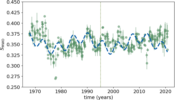
Figure 1: S-index ($S_{\mathrm{MWO}})$ vs time. Monthly averaged values are plotted as green circles, where the dispersion is shown as error bars. The dotted vertical line separates the $S_{\mathrm{MWO}}$ from this work (to the right of the vertical line) and Boro Saikia et al. (2018b) (to the left of the vertical line). The best fit cycle periods (22.3 and 5.7 years) from Boro Saikia et al. (2018b) are shown in blue.

One key disadvantage of the GLS algorithm or any other Fourier method is their ineffectiveness towards non-stationary signals, that is they are strong in period detection but do not provide temporal information of any detected periods. Additionally, in the case of a irregular non-sinusoidal period the harmonics might dominate over the true period. Wavelet analysis, on the other hand, can determine both the periodicities present in the signal and their duration and localisation in the time series. The specific wavelet analysis code used in this work is a modification of the one described in Torrence & Compo (1998). A Morlet function is used on a set of temporal scales and the wavelet is calculated for each scale, as well as the ‘cone of influence’ (COI) – the region of the wavelet spectrum in which edge effects (due to the fact that the time series are finite) become important. As discussed in Torrence & Compo (1998), the wavelet transform can be considered as a band-pass filter with a known response function, which filters the time series by summing over a subset of scales and also reconstructs the filtered signal. Here, we have chosen to use scales of less than 7 years, since most of the higher periodicities (even if real) will fall in the COI region (see Section 4.1). For determining the statistical significance of the filtered data and the probability level, we used the randomisation method described in detail in O’Shea et al. (2001).

3.2 Least squares deconvolution and Zeeman Doppler imaging

While $S_{\mathrm{MWO}}$ is a well studied magnetic activity proxy, detection of polarity reversals in the vector magnetic field is essential to constrain the star’s dynamo operated magnetic cycle (Petit et al., 2009; Fares et al., 2009; Boro Saikia et al., 2016; Mengel et al., 2016; Jeffers et al., 2018). We used the spectropolarimetric observations to determine the star’s large-scale magnetic field strength and geometry. We applied the technique of least squares deconvolution (LSD, Donati et al., 1997; Kochukhov et al., 2010) to boost the S/N of the observations, and used ZDI (Donati et al., 2006; Folsom et al., 2018) to reconstruct the large-scale surface magnetic field of $\kappa$ Ceti.

In Sun-like cool stars magnetic field signatures are extremely hard to detect in individual polarised spectral lines. Hence, we used the multi-line technique of LSD on our circularly polarised Stokes V and unpolarised Stokes I spectra (Donati & Brown, 1997; Kochukhov et al., 2010). To obtain an averaged LSD line profile we assumed that all magnetically sensitive lines in the observed spectra have the same characteristic shape. The final averaged LSD spectral line profiles were created by deconvolving the observed stellar spectra with a line mask. The line mask used in this work was taken from Marsden et al. (2014), which corresponds to a $T_{\mathrm{eff}}$ of 5750 K and a $\log g$ of 4.5. The mask was created from the Vienna Atomic Line Database (VALD, Kupka et al., 2000) using all lines that had a depth $\geq$ 10 percent of the continuum. Exceptionally broad lines such as Balmer lines were excluded from the mask. The normalisation parameters used for the LSD profiles were, a line depth of 0.52, a Landé factor of 1.22, and a central wavelength of 580 nm. The LSD (Stokes V) profiles for each epoch, containing a time series of 6-14 observations, are shown in Fig. 2 in black.

The tomographic technique of ZDI is an inverse routine that inverts observed LSD line profiles to reconstruct the large-scale surface magnetic geometry of stars. The version of ZDI used in this work (Folsom et al., 2018) uses a maximum entropy fitting, where model LSD line profiles are iteratively fit to observed LSD line profiles. The model LSD profiles for any given epoch were created using a spherical stellar model of $\kappa$ Ceti. All model stellar properties, except the radial velocity, were taken from the literature, as shown in Table 1. A simple Gaussian fit was performed on the observed LSD Stokes I profiles to determine the radial velocity of the star.

Table 1: Stellar properties of $\kappa$ Ceti.

Parameter	Value	Reference
Mass (M☉)	0.948	1
Radius (R☉)	0.917	1
Radial velocity, $v_{\mathrm{r}}$ (kms-1)	19.17	this work
Rotational velocity, $v\sin i$ (kms-1)	5.2	1
Rotation period, $P_{\mathrm{rot}}$ (days)	9.2	2
Inclination (o)	60	2
Age (Myrs)	750	3

(1) Valenti & Fischer (2005); (2) Rosén et al. (2016); (3) Güdel et al. (1997)

To create the model LSD line profiles our stellar model was divided into surface elements of equal area. Each surface element was assigned a local model line profile. The local model Stokes I lines are approximated as Voigt profiles and the local model Stokes V lines are created under the weak field approximation (Landi Degl’Innocenti & Landolfi, 2004). The model line profiles depend on the line-of-sight magnetic field strength, which in turn was calculated from a set of complex valued spherical harmonics coefficients ($\alpha_{\mathrm{lm}}$, $\beta_{\mathrm{lm}}$, and $\gamma_{\mathrm{lm}}$, where $l$ is the spherical harmonics degree and $m$ is the spherical harmonics order) that describe the magnetic field (Donati et al., 2006). The set of spherical harmonics were limited to a maximum degree $l_{\mathrm{max}}$ of 10 to be consistent with previous work by Rosén et al. (2016) and do Nascimento et al. (2016). Additionally, due to the low $v\sin i$ of the star increasing $l_{\mathrm{max}}$ to include higher degrees does not have any significant impact in the magnetic field reconstructions. The spherical harmonics coefficients are the free parameters during the fitting process and they define the three magnetic field vectors, radial $B_{\mathrm{r}}$, meridional $B_{\mathrm{\theta}}$, and azimuthal $B_{\mathrm{\phi}}$ (see Donati et al., 2006; Folsom et al., 2018, for more details). The final model LSD line profiles for a given observation were created by summing all the local line profiles from the visible surface area and scaled by a linear limb darkening law with a coefficient of 0.66. The final model LSD profiles were iteratively fit to the observed LSD profiles using the maximum entropy method (Skilling & Bryan, 1984). Figure 2 shows the best fit model LSD profiles in red.

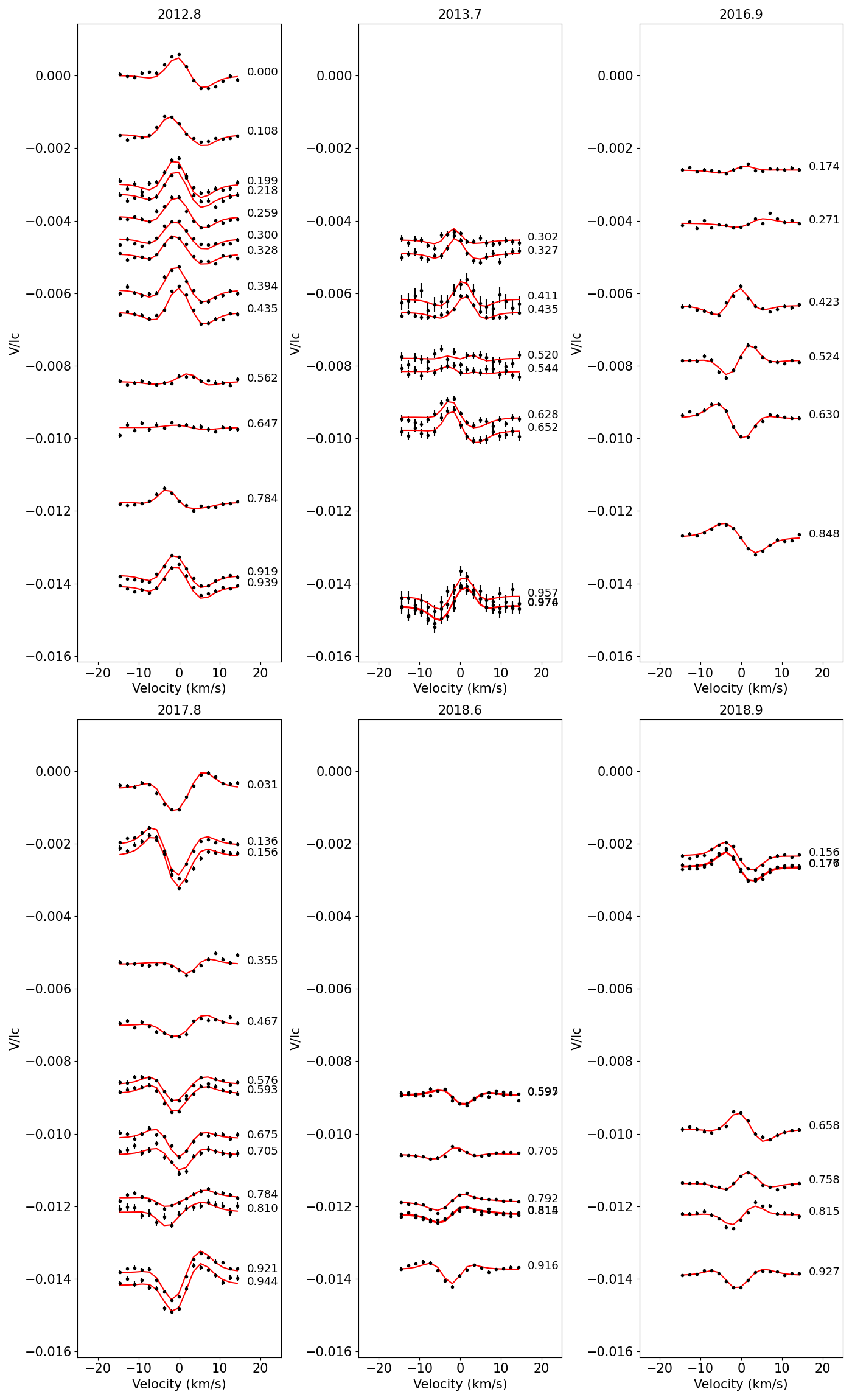
Figure 2: Observed (black) and modelled (red) Stokes V LSD profiles for the six epochs of observations. Rotational phases are shown next to each profile. The profiles are shifted vertically based on their rotational phases, where the phases increase from 0 to 1 (top to bottom).

The maximum entropy method is a regularisation routine that minimises the $\chi^{2}$ and maximises the entropy, and is an essential step for inverse problems such as ZDI. In this regularisation routine the user assigns a target $\chi^{2}$ known as $\chi^{2}_{\mathrm{aim}}$ that the routine aims to achieve by minimising $\chi^{2}$. Once $\chi^{2}=\chi^{2}_{\mathrm{aim}}$ is achieved the routine maximises the entropy till the maximum possible entropy is reached for $\chi^{2}=\chi^{2}_{\mathrm{aim}}$. The entropy definition is applied to the spherical harmonics coefficients $\alpha_{\mathrm{l,m}}$, $\beta_{\mathrm{l,m}}$, and $\gamma_{\mathrm{l,m}}$ which are the free parameters of the model. Table 2 lists the reduced $\chi^{2}$ achieved for the six epochs of observations. We do not include differential rotation in the ZDI reconstructions of the large-scale field, which could explain the slightly higher values of the reduced $\chi^{2}$. For a more detailed description of the ZDI technique and the regularisation routine please refer to Appendix B in Folsom et al. (2018).

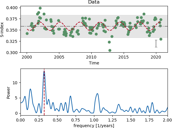
Figure 3: S-index of $\kappa$ Ceti over a 20 year time period in the top plot. The grey band marks the range of the solar S-index variability during a solar cycle. The 3.1 year cycle period is shown as a red dashed curve. The periodogram is shown in the bottom plot, where the strongest frequency is marked by a dashed red vertical line.

4 Results and discussion

4.1 Chromospheric activity cycles of $\kappa$ Ceti

The chromospheric activity ($S_{\mathrm{MWO}}$) of $\kappa$ Ceti is highly variable and exhibits multiple periodicities, as shown in Fig. 1. In a previous study we identified two chromospheric activity cycles with a period of 22.3 years and 5.7 years using the GLS periodogram (Boro Saikia et al., 2018b). The blue dashed line in Fig. 1 represents the two activity cycles, and they are in good agreement with the observed $S_{\mathrm{MWO}}$ measurements from the late 1970s to the early 2000s. However, the agreement between the two detected cycle periods and the $S_{\mathrm{MWO}}$ measurements is weaker in the very early parts and the later half of the time series, as shown in Fig. 1. This could be either due to variable duration of one or both cycle periods, complex temporal evolution of the cycles, presence of multiple other periodicities that dominate in the beginning and the later part of the time series, or any combination of the above.

To investigate this further, we applied the GLS periodogram on the new observations (2000-2020), which is a sub-set of the time series in Fig 1. The strongest peak of the periodogram lies at 3.1$\pm$0.01 years, as shown in Fig. 3. The FAP of this cycle period is $1.3\mathrm{e-}05$, which is not as robust as the 5.7 year (FAP = $6.3\mathrm{e-}51$) cycle period in Boro Saikia et al. (2018b). While the 3.1 year could be a harmonic of the 5.7 ($\sim$ 6) year period, we could not detect the 22.3 year period which could be due to the shorter time series of 20 years. On closer inspection of Fig. 1, the overall trend in the later part of the time series (2000 onwards) appears to be more flat compared to the pre-2000 time series, which could also contribute to the lack of detection of the longer 22.3 year period.

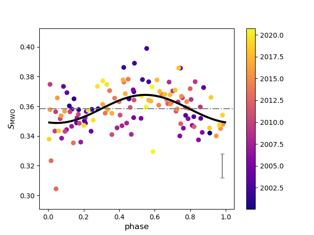
Figure 4: Same S-indices as Fig. 3, but the data were phase-folded using a cycle period of 3.1 years (in black). The colour bar represents the observational time-span in years.

The period analysis on the shorter data set (2000-2020) in Fig. 3 shows that the dominant cycle period has a duration of 3.1 years. However, this period on its own does not explain the complex variability in the data set. This is clearly seen in the phase-folded S-indices in Fig. 4, where the data shows a weak agreement with the 3.1 year cycle period. The complexity of $\kappa$ Ceti’s S-index variability lies far beyond the cycle periods identified by the GLS periodogram and information on the temporal evolution of its cycle periods is needed.

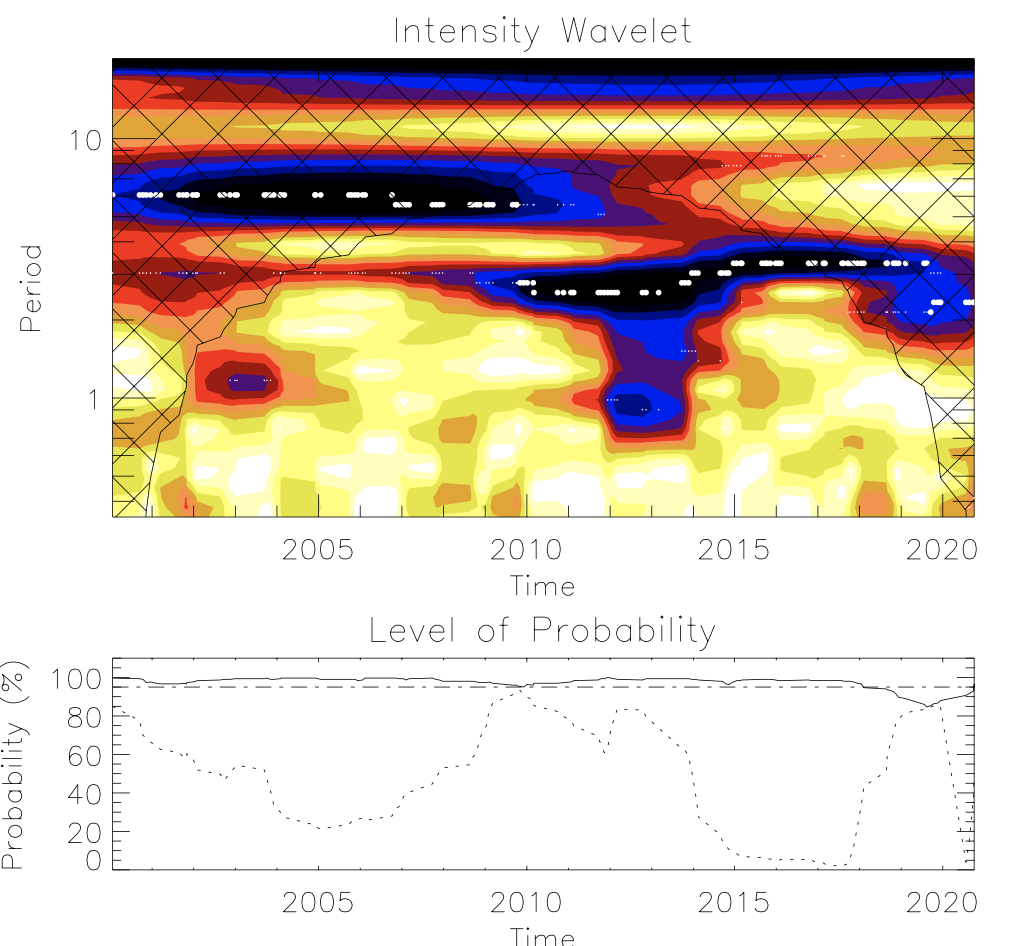
Figure 10: Same as Fig. 5, but only for the new data set between 2000-2020. The solid line represents the probability level for the 3.1 year period and the dotted line shows the probability level of the 5.7 year period.

We applied a wavelet transform to $\kappa$ Ceti’s monthly averaged $S_{\mathrm{MWO}}$ measurements, as described in Section 3.1. Our wavelet code detected two dominant cycle periods of 5.8 years and 3.1 years including their occurrence in time, with a probability level of $99\%-100\%$ for the two detected periods, as shown in Fig. 5. The 22.3 years cycle detected using the GLS periodogram in Boro Saikia et al. (2018b) falls inside the COI of our transform and is not included in this work. The COI, shown as a cross-hatched area in Fig. 5, marks the region within which the period determination is unreliable, due to edge-effects and limited time series length (Torrence & Compo, 1998). The 5.8 cycle period in Fig. 5 is in good agreement with the 5.7 year cycle period determined from monthly averaged measurements in Boro Saikia et al. (2018b), and it is the only dominant cycle period between early 1980’s and mid 2000’s, as shown in Fig. 5. In the first $\sim$10 years of the time series, the 3.1 year cycle co-exists with the 5.8 year cycle, where as the 3.1 year cycle is the only dominant cycle period from $\sim$2008 onwards. A wavelet decomposition on the 2000-2020 data set also shows that the 3.1 year is the dominant cycle period during this period (Fig. 10).

Over a time period of 50 years the chromospheric activity of $\kappa$ Ceti exhibits two strong periodicities with variable temporal evolution. The $\sim$1:2 ratio between the two periods suggest that the 3.1 year period is the first harmonic. This shows the importance of long-term monitoring of stellar activity data, specially for active young Suns with highly irregular chromospheric activity. Based on when the star is observed one would only detect the 3.1 year cycle period, with a non-detection of the 5.7-5.8 (referred as the 5.7 from here onwards) year period, as shown in Figures 3 and 10.

Multiple cycle periods have been also detected in a limited number of Sun-like stars (Baliunas et al., 1995; Oláh et al., 2016). As an example, a wavelet decomposition on the active exoplanet-host star $\epsilon$ Eridani by Metcalfe et al. (2013) suggests a possible $\kappa$ Ceti-like behaviour of the star’s two dominant cycles. Recent multi-wavelength observations of $\epsilon$ Eridani by Coffaro et al. (2020) and Petit et al. (2021) indicates that the star’s magnetic activity is approaching a more chaotic regime. Period analysis of long-term stellar activity measurements will help us determine if such complex evolution of multiple activity cycles is indeed a common occurrence in young Suns.

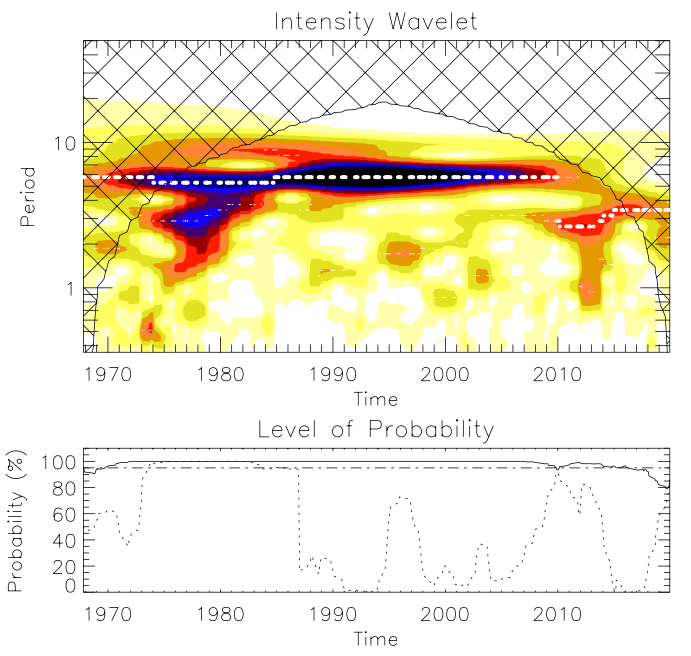
Figure 5: Top: Wavelet intensity spectrum of monthly averaged $S_{\mathrm{MWO}}$ of $\kappa$ Ceti. The strongest cycle periods are represented by the darker colours and the dashed horizontal white lines, and the cross-hatched area shows the COI. Bottom: The probability associated with the two detected periods of 5.8 (solid black line) and 3.1 (dotted black line) years. The 90$\%$ probability level is shown as a horizontal dashed and dotted line.

Table 2: Reduced $\chi^{2}$ of the ZDI magnetic maps.

epoch	$\chi^{2}$
2012.8	1.5
2013.7	1.0
2016.9	1.1
2017.8	1.3
2018.6	1.1
2018.9	1.2

Even a moderately active cool star such as our Sun exhibits multiple periodicities in its activity and magnetic field measurements. The most prominent and well studied solar cycle is the sunspot cycle, also known as the Schwabe cycle, which exhibits a periodicity of 11${{}^{+3}_{-2}}$ years (Usoskin, 2017). The 11 year Schwabe cycle is closely tied to the 22 year magnetic cycle or Hale cycle, where the global magnetic field of the Sun flips its polarity. The Hale and Schwabe cycles have a 1:2 ratio, and are tied to the underlying tachocline dynamo of the Sun. On the surface $\kappa$ Ceti’s 3.1 and 5.7 year cycles also exhibit a $\sim$1:2 ratio similar to the two dominant solar cycles. However, $\kappa$ Ceti’s cycles exhibit a far more complex behaviour. While the 5.7 year cycle dominates for the majority of the time series, it gets considerably weaker in the later part of the time series, as shown in Fig.5. This is a stark difference from the behaviour of the two dominant solar cycles. Furthermore, for reliable comparison with the solar Hale and Schwabe cycles one must have information on $\kappa$ Ceti’s magnetic field polarity flips.

Based on the chromospheric activity data alone the complex evolution of $\kappa$ Ceti’s two strong cycle periods could be attributed to strong stellar surface inhomogeneities. As an example, the Sun also exhibits multiple other periodicities apart from the two dominant cycles mentioned above. The most prominent of which is the Gleissberg cycle of $\sim$90 years (Gleissberg, 1939), which exhibits significant variations in amplitude and duration. The Gleissberg cycle is associated with sunspot appearance and is shown to have existed for at least within the last millennia (Ogurtsov et al., 2002), although it is known to sometimes completely disappear (Beer et al., 2018). Investigations of the north-south asymmetries of magnetic activity in the Sun have also resulted in the detection of a cycle period similar to the Gleissberg cycle and multiple other short term cycle periods (Deng et al., 2016). However, the amplitudes of the multiple periods detected in $\kappa$ Ceti are much stronger than in the multiple periods detected in the solar case. Hence additional measurements of the photospheric vector magnetic field of $\kappa$ Ceti is crucial to reliably characterise the two cycles in Fig. 5.

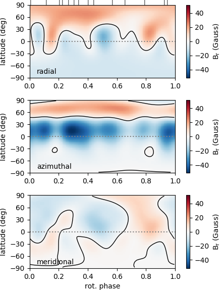
(a) 2012.8

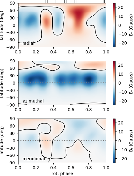
(b) 2013.7

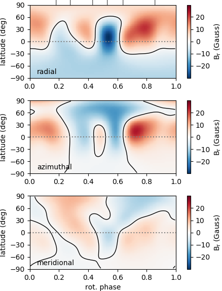
(c) 2016.9

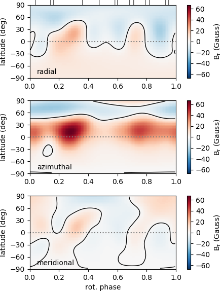
(d) 2017.8

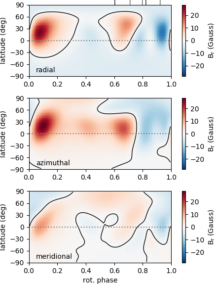
(e) 2018.6

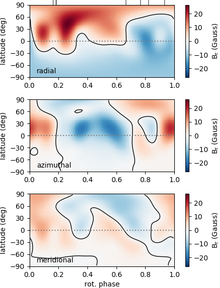
(f) 2018.9

Figure 6: Surface magnetic maps of $\kappa$ Ceti for six observational epochs. The large-scale radial, azimuthal and meridional field is shown in each sub-plot. The rotational phase is shown in the x-axis and the latitude is shown in the y-axis. The equator is marked by a horizontal dotted line. The magnetic field strength is shown in gauss, where red denotes positive polarity and blue denotes negative polarity. The black tick marks at the top mark the observed rotational phases. The colour scale is determined based on the maximum magnetic field strength in each ZDI map.

4.2 Magnetic field geometry and polarity flips

Reconstructions of the large-scale surface magnetic field geometry were carried out using the technique of ZDI for six observational epochs. Figure 6 shows the ZDI surface magnetic maps for the vector magnetic field in the three directions, radial, azimuthal, and meridional. The meridional field is much weaker than the radial and the azimuthal field, as shown in Fig. 6 (bottom panels). It has been shown by previous studies that possible cross-talk between the radial and meridional components lead to underestimation of the latter (Donati & Brown, 1997; Rosén et al., 2015; Lehmann et al., 2019). Hence we only discuss the properties of the radial and the azimuthal field. By definition the radial component of the magnetic field relates to the poloidal magnetic field and the azimuthal and meridional components of the magnetic field relate to both poloidal and toroidal component of the magnetic field (See Donati et al., 2006; Folsom et al., 2018, for more details).

4.2.1 Radial field

The radial field of $\kappa$ Ceti exhibits considerable evolution over a six year period, as shown in Fig. 6 (top panels). A positive polarity radial magnetic field dominates the northern hemisphere of the star at epoch 2012.8. At epoch 2013.7 and 2016.9 the positive polarity is not as dominant as in epoch 2012.8 and the northern hemisphere consists of both strong positive and negative magnetic field. A negative polarity magnetic field takes over at epoch 2017.8, indicating a polarity flip from positive to negative. The radial field undergoes a reconfiguration a year later at epoch 2018.6 exhibiting a mixed polarity in the northern hemisphere. At epoch 2018.9 the mixed polarity evolves to show a stronger positive polarity magnetic field. Although the sparse phase coverage of epochs 2018.6 and 2018.9 make it difficult to obtain robust magnetic maps, the Stokes V profiles in Fig 2 show considerable variation in the amplitude and signature, providing confidence that the magnetic field undergoes a rapid evolution towards the end of our observational time-span.

The evolution of the radial magnetic field component shows strong evidence of a polarity flip from 2012.8 to 2017.8, indicating it could take 5 years for the star’s large-scale radial magnetic field to flip polarity. In those five years (between 2012.8 and 2017.8) only two other (2013.7 and 2016.9) magnetic maps are available. At epoch 2013.7 the radial field exhibits both positive and negative polarity regions, indicating a much more complex field than a year earlier at epoch 2012.8. Epoch 2016.9 also shows a complex magnetic field, with the presence of both negative and positive polarities in the northern hemisphere, so the only other time the star could have undergone a polarity switch from a positive to a negative magnetic field before 2017.8 is between 2013.7 and 2016.9. This will suggest that the dominant positive magnetic field in 2012.8 flips to a dominant negative field between 2013.7 and 2016.9, and turns back to positive in 2017.8, resulting in a magnetic or Hale cycle of $\sim$ 6 years. However, Fig 6 shows that at epoch 2017.8 the radial field is dominantly negative not positive as expected, indicating that the $\sim$ 6 year Hale cycle is not feasible.

Based on our observations, the flip in 2017.8 is most likely the first polarity flip between epoch 2012.8 and 2017.8, and we expect the Hale cycle to have a period of $\sim$10 years. Since a majority of our observations were taken at yearly epochs any polarity flips that might have occurred at monthly intervals were missed. Future high cadence observations will help us fully characterise the Hale cycle.

4.2.2 Azimuthal field

The azimuthal field evolves from a simple almost single polarity field to a more complex field during the course of our observations, as shown in Fig. 6 (middle panels). It exhibits a band of strong negative polarity field at equatorial latitudes at epochs 2012.8 and 2013.7. Over time the field evolves, with the appearance of a positive polarity magnetic field at epoch 2016.9, which switches to a dominant positive polarity magnetic field at epoch 2017.8. The dominant positive polarity azimuthal field re-configures at epoch 2018.6, with the appearance of negative polarity regions. Epoch 2018.9 shows the presence of both positive and negative large-scale magnetic field.

Table 3: Magnetic properties.

epoch	Bmean (G)	pol ($\%$total)	dipole ($\%$poloidal)	quad ($\%$poloidal)	oct ($\%$poloidal)	axi ($\%$total)
2012.8	21$\pm$2	30$\pm$5	44$\pm$8	17$\pm$3	15$\pm$3	74$\pm$2
2013.7	11$\pm$1	36$\pm$1	37$\pm$4	27$\pm$1	22$\pm$2	64$\pm$2
2016.9	12$\pm$1	85$\pm$3	51$\pm$4	14$\pm$2	23$\pm$3	25$\pm$3
2017.8	20$\pm$1	26$\pm$1	24$\pm$5	43$\pm$4	13$\pm 1$	74$\pm$1
2018.6	9$\pm$1	77$\pm$1	18$\pm$1	43$\pm$2	20$\pm$2	19$\pm$2
2018.9	12$\pm$1	81$\pm$3	71$\pm$2	12$\pm$3	5$\pm$1	25$\pm$3

While the single polarity positive radial field changes to a more complex field from 2012.8 to 2013.7, the azimuthal field primarily remains at a single polarity from 2012.8 to 2013.7, as shown in Fig. 6. This discrepancy between the radial and the azimuthal field could be explained by a time lag between the azimuthal field and the radial field. A time lag of 1-3 years is known to exist between the solar poloidal and toroidal magnetic fields (Cameron et al., 2018). A time lag between the radial and the azimuthal field is also detected in the case of other Sun-like stars (Jeffers et al., 2018; Boro Saikia et al., 2018a). Taking this time lag into account, the azimuthal field is in good agreement with the radial field suggesting it also undergoes a polarity reversal. However this time lag is not detected from 2017.8 to 2018.6, which suggests our epochs are too sparse to fully explore the complexity of $\kappa$ Ceti’s magnetic field evolution.

4.3 Magnetic morphology

The large-scale ZDI magnetic geometry of $\kappa$ Ceti is composed of both poloidal and toroidal field components, with the poloidal field dominating in epochs 2016.9, 2018.6, and 2018.9, and the toroidal field dominating in epochs 2012.8, 2013.7, and 2017.8, as shown in Table 3. The strong toroidal field corresponds to the appearance of the single polarity equatorial azimuthal field at epochs 2012.8, 2013.7, and 2017.8 in Fig. 6. It is not surprising as young cool dwarfs like $\kappa$ Ceti are known to switch from dominantly poloidal to toroidal configuration over multi-epoch observations (Petit et al., 2008; Boro Saikia et al., 2015; Rosén et al., 2016; See et al., 2015). Although, exceptions exists as the young solar analogue $\epsilon$ Eridani exhibits a consistently strong poloidal field over multiple epochs with a stronger toroidal field in only one out of nine epochs (Jeffers et al., 2014, 2017). Whereas, a dominantly toroidal field is detected in the young Sun EK Dra over five epochs (Waite et al., 2017). Our Sun and older cool stars like 61 Cyg A (Boro Saikia et al., 2016) exhibit a dominant surface poloidal field.

The percentage of magnetic energies distributed between the different components of the star’s poloidal magnetic field is shown in Table 3. The poloidal field is strongly dipolar ($l$=1) at certain epochs, whereas the quadrupolar ($l$=2) field dominates at other epochs. Since the large-scale field is made up of both poloidal and toroidal components we also investigate the fraction of magnetic energy in the lower spherical harmonics order of the poloidal and toroidal field ($l$ = 1, 2, 3). Figure 7 shows that at all observed epochs $\geq$80$\%$ of the total energy (combined poloidal and toroidal) can be found in the lower order spherical harmonics degree $l$=1, 2 and 3.

No clear periodicity is detected in the fluctuations in the magnetic energies associated with the lower order harmonics, as shown in Fig. 7. According to Lehmann et al. (2021) periodicities are not easily detectable in the magnetic energy fractions of ZDI magnetic maps. Instead, the authors identified the axisymmetric fraction as a good tracer of the magnetic cycles. Although the axisymmetric fractions do not show any clear periodic behaviour, as shown in Table 3 a weak anti-correlation between its strength and the percentage of the poloidal energy is detected.

Similar to the analysis of Rosén et al. (2016) and do Nascimento et al. (2016), our results show that the majority of the magnetic energy is concentrated in the lower harmonic degrees. However, slight discrepancies between the magnetic properties derived in this work and Rosén et al. (2016) are also detected, specifically for the HARPSpol data at epoch 2013.7. At epoch 2013.7 the magnetic field strength determined in this work is a factor of 2 weaker than the field strength obtained by Rosén et al. (2016). This discrepancy could be attributed to differences in the line mask used for LSD, the stellar line models, and the definition of the maximum entropy used in the ZDI code. Such differences might be of greater importance for the high-resolution spectropolarimetric data taken by HARPSpol, as no such discrepancy is detected in the 2012.8 data. Despite the differences in the mean magnetic field strength at epoch 2013.7 our reconstructed magnetic geometry in Fig. 6 is in strong agreement with the magnetic map in Rosén et al. (2016). Hence, we are confident that the large-scale magnetic map of 2013.7 can be utilised to monitor the polarity reversal of the star.

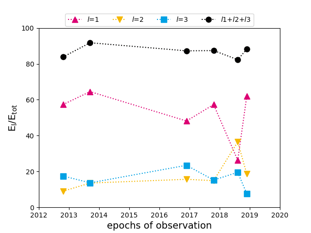
Figure 7: Magnetic energies (poloidal+toroidal) for the three smallest values of spherical harmonic degree $l$.

4.4 The relation between magnetic polarity flips and chromospheric activity cycle

The ZDI magnetic maps of $\kappa$ Ceti exhibit polarity reversals of the radial and the azimuthal magnetic field over a six year time-span. As shown in Fig. 8, during this time period the star would undergo at least two 3.1 year (shorter) chromospheric cycles and one 5.7 year (longer) cycle. Depending on which cycle period one considers only two/one ZDI maps were observed at an activity maximum (3.1 year period/5.7 year period), none were observed at activity minimum, and the rest were observed in between activity minimum and maximum.

Figure 8 shows that irrespective of which cycle period one considers the star’s magnetic evolution deviates from the solar case. In the Sun a complex magnetic field appears on the surface during solar cycle maximum and the magnetic field changes polarity from one cycle minimum to the next (Hathaway, 2010; DeRosa et al., 2012). However in the case of $\kappa$ Ceti, the polarity flips do not occur from one minimum to the next. Although, the complexity of the two maps (appearance of bipolar magnetic regions) observed during activity maxima increases compared to the other epochs. Reconstructing its magnetic field geometry during cycle minima will provide stronger constraints on $\kappa$ Ceti’s magnetic cycle evolution.

Future high cadence observations of this star could help us understand the true relationship between the magnetic polarity flips and the chromospheric cycles.

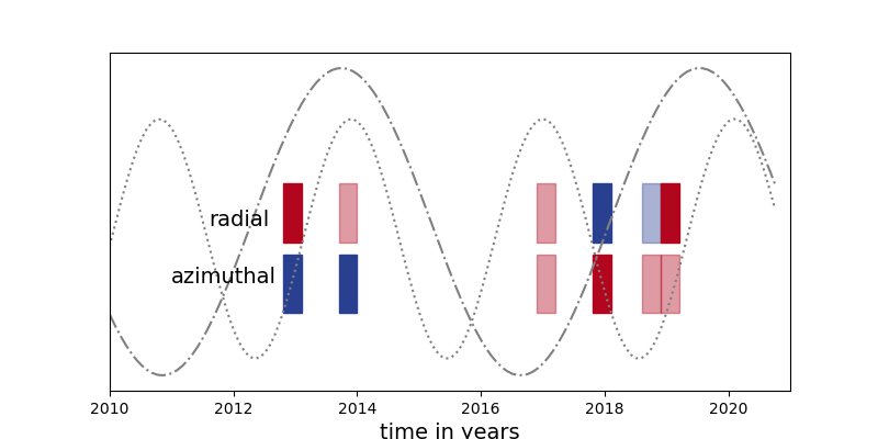
Figure 8: Relation between the 5.7 year (dotted and dashed grey curve) and 3.1 year (dotted grey curve) chromospheric activity cycles, and the polarity reversals in the radial (top row of rectangles) and azimuthal magnetic field (bottom row of rectangles). The red rectangles represent dominant positive polarity magnetic field and the blue rectangles represent dominant negative polarity magnetic field. The transparent rectangles mark epochs when additional opposite polarity magnetic regions are also detected in addition to the dominant polarity.

As an example, in the case of the planet hosting star $\tau$ Boo, initial multi-epoch observations at yearly intervals suggested a $\sim$2 year magnetic cycle (Donati et al., 2008; Fares et al., 2009, 2013), at an 1:3 ratio with the star’s chromospheric cycle (Mengel et al., 2016; Mittag et al., 2017). Additional spectropolarimetric observations of the star at monthly intervals by Jeffers et al. (2017) confirmed that its large-scale magnetic field reverses polarity more frequently, leading to a magnetic cycle of 240 days. The authors also detected an increase in complexity of $\tau$ Boo’s magnetic field as it approaches chromospheric activity maximum.

With a rotation period of 9.2 days, $\kappa$ Ceti is a moderately rotating young Sun for its age, as shown by stellar rotational evolution models (Gallet & Bouvier, 2013; Johnstone et al., 2015). Until now the magnetic field evolution of only one other moderately rotating young Sun, $\epsilon$ Eridani, has been investigated using both chromospheric activity and ZDI magnetic maps over multiple epochs. Long-term monitoring of $\epsilon$ Eridani shows the presence of two chromospheric cycle periods (Metcalfe et al., 2013). However, recent investigations on the star’s chromospheric measurements suggest a complex activity with the disappearance of the star’s longer cycle period (Coffaro et al., 2020; Petit et al., 2021), indicating strong similarities with $\kappa$ Ceti’s chromospheric activity evolution. The large-scale magnetic field evolution of $\epsilon$ Eridani is more complex than that of $\kappa$ Ceti, although there is indication of a possible polarity switch in the dipole field (Jeffers et al., 2014, 2017; Petit et al., 2021). There is a strong possibility that both $\kappa$ Ceti and $\epsilon$ Eridani reflect a magnetic evolution that is unique to moderately rotating young Suns. High-cadence spectroscopic and spectropolarimetric observations could help us correctly constrain the evolution of $\kappa$ Ceti’s large-scale field, which will be addressed in a future work .

5 Summary and conclusions

The multi-epoch spectroscopic and spectropolarimetric observations carried out in this work enabled us to provide an in-depth analysis of the complex magnetic variability of the young Sun $\kappa$ Ceti. The key conclusions are discussed below.

• The chromospheric activity measurements of $\kappa$ Ceti over $\sim$50 years indicate the presence of two activity cycles with a 1:2 ratio similar to the Schwabe and the Hale cycle. However, unlike the solar cycles the 3.1 and 5.7 year cycle periods show a complex temporal evolution. While the longer cycle dominates for a good portion of our time series, the shorter cycle period is appears in the very early and later part of the data set. Similar complex chromospheric variability is also reported for another moderately rotating young star $\epsilon$ Eridani. Our results suggest that such complex evolution of magnetic activity could be synonymous with moderately active young Suns, an evolutionary path that our own Sun could have taken.

• Our ZDI reconstructions show that the radial and azimuthal directions of the field undergo polarity reversals, indicating a potential Solar-like dynamo cycle, with a cycle period of $\sim$10 years. However, the exact length of the cycle period could vary by a year or two, as our current spectropolarimetric observations do not have a high cadence or a long time-baseline.

• Magnetic polarity reversals in correlation with chromospheric activity is one of the best known ways of constraining the dynamo cycle a Sun-like star. For a solar-type dynamo the magnetic polarity reversals should coincide with the activity cycle minima, followed by the appearance of a complex field during activity maxima. Although $\kappa$ Ceti’s magnetic field appears to be more bipolar during activity maxima, the polarity reversals are out of sync with the cycle minima. Our multi-epoch monitoring suggests that the star’s magnetic cycle deviates from the Sun-like polarity reversals. Further high cadence spectroscopic and spectropolarimetric observations of cool stars will be crucial in determining if the magnetic field in moderately rotating young Solar analogues indeed evolve differently from the current Sun.

Appendix A

Figure 9: Individual $S_{\mathrm{MWO}}$ measurements of $\kappa$ Ceti between 1966-2020. The different colours mark the data sources.

1]

Appendix B Journal of observations.

Table 4: Journal of spectropolarimetric observations taken at HARPSpol (2013.7) and NARVAL/TBL (2012.8, 2016.9, 2017.8, 2018.6, 2018.9).

Epoch	date	Julian date	$\sigma_{\mathrm{LSD}}$	rotational
		(2450 000+)	10${}^{-5}I_{\mathrm{c}}$	cycle
	01 October 2012	6202.52180	4.8	0.000
	02 October 2012	6203.51912	3.8	0.108
	03 October 2012	6204.52650	6.8	0.218
	04 October 2012	6205.53850	4.2	0.328
	05 October 2012	6206.52522	4.9	0.435
	12 October 2012	6213.55626	7.0	1.199
	13 October 2012	6214.48132	4.5	1.300
2012.8	23 October 2012	6224.54605	6.2	2.394
	28 October 2012	6229.55813	4.9	2.939
	31 October 2012	6232.50488	5.1	3.259
	06 November 2012	6238.57330	4.1	3.919
	12 November 2012	6244.49623	5.8	4.562
	14 November 2012	6246.53620	4.3	4.784
	22 November 2012	6254.47162	6.6	5.647
	09 September 2013	6545.7018	9.5	37.302
	09 September 2013	6545.9281	8.6	37.327
	10 September 2013	6546.7004	20.1	37.435
	10 September 2013	6546.9248	6.5	37.411
	11 September 2013	6547.7017	11.5	37.544
2013.7	11 September 2013	6547.9248	10.8	37.520
	12 September 2013	6548.7013	9.1	37.628
	12 September 2013	6548.9226	11.7	37.652
	15 September 2013	6551.7258	15.9	37.957
	15 September 2013	6551.8868	12.6	37.974
	15 September 2013	6551.8980	17.5	37.976
	01 November 2016	7694.51937	5.0	162.174
	02 November 2016	7695.41739	4.6	162.271
	01 December 2016	7724.41020	5.7	165.423
2016.9	02 December 2016	7725.33896	5.1	165.524
	03 December 2016	7726.31571	4.9	165.630
	05 December 2016	7728.32758	4.7	165.848
	26 September 2017	8023.60956	7.8	197.944
	28 September 2017	8025.55739	7.6	198.156
	02 October 2017	8029.57291	6.3	198.593
	03 October 2017	8030.61015	8.0	198.705
	04 October 2017	8031.57700	10.3	198.810
	05 October 2017	8032.59530	5.3	198.921
2017.8	06 October 2017	8033.61134	5.2	199.031
	07 October 2017	8034.57082	4.9	199.136
	09 October 2017	8036.58561	5.8	199.355
	10 October 2017	8037.61879	5.3	199.467
	11 October 2017	8038.61716	5.6	199.576
	12 October 2017	8039.53068	6.8	199.675
	13 October 2017	8040.53481	5.6	199.784
	20 August 2018	8351.59545	3.9	233.597
	20 August 2018	8351.61006	5.2	233.595
	21 August 2018	8352.60425	4.2	233.705
2018.6	22 August 2018	8353.60739	3.6	233.815
	22 August 2018	8353.62129	4.9	233.814
	23 August 2018	8354.54734	5.0	233.916
	31 August 2018	8362.60629	2.9	234.792
	24 October 2018	8416.57808	5.6	240.658
	25 October 2018	8417.49351	2.9	240.758
	07 November 2018	8430.53761	5.1	242.177
2018.9	07 November 2018	8430.55348	3.3	242.176
	13 November 2018	8436.42431	5.2	242.815
	14 November 2018	8437.44667	3.2	242.927
	16 November 2018	8439.55539	4.2	243.156

Table 4: continued.