DiscoDVT: Generating Long Text with Discourse-Aware Discrete Variational Transformer

Abstract

Despite the recent advances in applying pre-trained language models to generate high-quality texts, generating long passages that maintain long-range coherence is yet challenging for these models. In this paper, we propose DiscoDVT, a discourse-aware discrete variational Transformer to tackle the incoherence issue. DiscoDVT learns a discrete variable sequence that summarizes the global structure of the text and then applies it to guide the generation process at each decoding step. To further embed discourse-aware information into the discrete latent representations, we introduce an auxiliary objective to model the discourse relations within the text. We conduct extensive experiments on two open story generation datasets and demonstrate that the latent codes learn meaningful correspondence to the discourse structures that guide the model to generate long texts with better long-range coherence.

1 Introduction

Generating passages that maintain long-range coherence is a long-standing problem in natural language generation (NLG). Despite the recent advances of large pre-trained language generation models (Radford et al., 2019; Lewis et al., 2020) in various NLG tasks such as summarization and dialogue generation that target generating locally coherent texts which are relatively short, it is still challenging for pre-trained models to generate globally coherent passages spanning over dozens of sentences.

Global coherence in human texts is represented by the topic-maintenance and natural transition between viewpoints (Jurafsky and Martin, 2000). As illustrated in Figure 1, discourse relations such as causal, temporal succession between contiguous text segments are commonly indicated by the highlighted discourse markers which bind collocated text segments into a global structure (Hobbs, 1985). Although pre-trained language models are inspected to perform reasonably well in associating topic-related concepts, they can hardly arrange contents with well-structured discourses (See et al., 2019; Ko and Li, 2020).

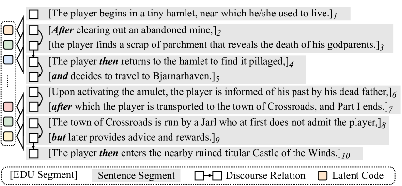
Figure 1: An example from Wikiplots where a discrete latent variable sequence abstracts the discourse structure of the text. Inter-sentence and intra-sentence discourse relations are indicated by the bolded discourse markers.

In this work, we urge the revival of variational autoencoder (VAE) with its global representation ability to tackle the incoherence issue in long text generation in the era of pre-trained language models. To represent texts with high-level structures, we propose to learn a latent variable sequence with each latent code abstracting a local text span. Instead of the commonly used continuous latent variables, we resort to learn discrete latent codes that naturally correspond to interpretable categories in natural languages (Zhao et al., 2018). For the latent codes to capture the explicit discourse structure of the texts as shown in Figure 1, we further design an auxiliary objective on the latent representations to model the discourse relations.

We name the proposed model as DiscoDVT, i.e., Discourse-aware Discrete Variational Transformer. The main idea is to learn a discrete latent variable sequence that summarizes the long text to reconstruct the original text by guiding the decoding process. The learning schema is shown in Figure 2 (a). At the encoding phase, to capture the high-level structure of the text, we first use a bidirectional encoder to obtain contextualized token representations and then apply 1-dimensional convolutional neural networks (1D CNNs) to abstract text segments at the temporal scale (§3.2.1). To condense the continuous representations into categorical features, we map them into a one-hot categorical distribution over a fixed latent vocabulary, and obtain the discrete variable sequence (§3.2.2). At the decoding phase, to apply the global discrete latent codes to guide the local text realization, the latent embeddings are first rescaled to the text length with transposed 1D CNNs, and then added to the embedding layer of the decoder for step-wise control (§3.2.3). For the latent codes to abstract the discourse structure of the text, we use explicit discourse relations from Penn Discourse TreeBank 2.0 (PDTB, Prasad et al., 2008) and extract adjacent elementary discourse units (EDUs) from texts as shown in Figure 1 and introduce an anxiliary objective to embed the relations into the latent representations. Once the discrete latent codes are learned, we adopt an autoregressive Transformer to model the prior distribution as a sequence transduction task (§3.4).

We summarize our contributions in three folds:

(1) We propose a novel latent variable model that learns discrete latent variable sequence from the long text and applies it to guide the generation process to maintain long-term coherence.

(2) We further acquire the discourse relation information and introduce an auxiliary objective for the discrete latent codes to abstract the discourse structure of the text.

(3) We conduct extensive experiments on two open story generation datasets with automatic and human evaluation. Results demonstrate that our model outperforms baselines in generating coherent long texts with interpretable latent codes.

2 Related Work

2.1 Long Text Generation

Prior works endeavored to solve the incoherence issue in long text generation can be mainly categorized into model structure modifications, generation mechanism modifications, and prior knowledge injection.

To model the hierarchical nature of human texts, Li et al. (2015) proposed a hierarchical RNN decoder to learn sentence-level representations within the paragraph. Shen et al. (2019) augmented the hierarchical model with multi-level latent variables, and Shao et al. (2019) further incorporates a planning mechanism to pre-arrange the order and the group of the input keywords.

Another line of works proposed to decompose long text generation into multiple stages (Fan et al., 2018; Yao et al., 2019; Fan et al., 2019; Tan et al., 2020) where the model first generates a rough sketch, such as key phrases or summaries, and then expands it into the complete long text with fine detail. However, the multi-step generation method is known to have the stage-level exposure bias (Tan et al., 2020), i.e., the discrepancy of middle-stage outputs during training and inference, which can accumulate error through stages and impair the final generation quality.

The final direction is to inject prior external knowledge into pre-trained language models for commonsense story generation (Guan et al., 2020; Xu et al., 2020). However, these methods may not be generalizable to different data genres such as fictional stories and do not provide long-range guidance during text generation.

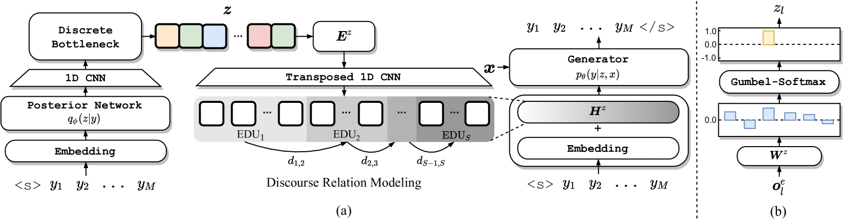
Figure 2: Overview of DiscoDVT. (a) Learning discrete latent codes via encoding and reconstructing the target text with discourse relation modeling where the latent representations are required to predict discourse relations within the text. (b) The discrete variational bottleneck maps the output of the encoder into a categorical distribution over a fixed latent vocabulary.

2.2 Discrete Latent Variable Models

In text generation, continuous Gaussian VAEs have been explored to model response diversity (Zhao et al., 2017; Serban et al., 2017) and high-level structures, such as template and order (Wiseman et al., 2018; Shen et al., 2019; Shao et al., 2019). Aside from Gaussian latent variables in the continuous space (Kingma and Welling, 2014), recent works also explored VAEs in the discrete space (Rolfe, 2017) with the merit of explainability and revealed the correspondence between the latent codes and categorical features, e.g., dialogue acts (Zhao et al., 2018) and POS tags (Bao et al., 2021). Recently, van den Oord et al. (2017) proposed a vector-quantized variational autoencoder (VQ-VAE) which circumvents the posterior collapse problem by learning quantized one-hot posterior that can be adapted with powerful autoregressive decoders. In image and speech generation, Razavi et al. (2019); Dieleman et al. (2018) extended VQ-VAE with hierarchical latent variables to capture different input data resolutions and generate high-fidelity visual and audio data with high-level structures. To our knowledge, in the domain of text generation, our work is the first attempt that explores discrete latent variable models scaling up to the size of large pre-trained language models to solve the incoherence issue in long text generation.

3 Methodology

3.1 Task Definition and Model Overview

We formulate the long text generation task as a conditional generation problem, i.e., generating a multi-sentence text $\boldsymbol{y}=(y_{1},\cdots,y_{M})$ given an input prompt $\boldsymbol{x}=(x_{1},\cdots,x_{N})$. Current pre-trained generation models, e.g., BART, adopt Transformer-based encoder-decoder structure that bidirectionally encodes $\boldsymbol{x}$ and maximizes the log-likelihood $\mathcal{L}_{\text{LM}}$ of predicting $\boldsymbol{y}$ at the decoder side.

However, existing models can hardly maintain long-range coherence when generating long texts that span hundreds of words. We propose to learn a discrete sequence of latent variables $\boldsymbol{z}=(z_{1},\cdots,z_{L})$ to abstract the high-level structure of the text at the temporal scale ($L$ is much shorter than $M$) and categories (each $z_{l}$ takes value from the latent vocabulary with size $K$, which is much smaller than the text vocabulary).

Our model maximizes the evidence lower bound (ELBO,  Kingma and Welling, 2014) of the log-likelihood of the generative model: $p(\boldsymbol{y},\boldsymbol{z}|\boldsymbol{x})=p_{\theta}(\boldsymbol{y}|\boldsymbol{z},\boldsymbol{x})p_{\psi}(\boldsymbol{z}|\boldsymbol{x})$ where the generator and the prior network are parametrized by $\theta$ and $\psi$, respectively. Since we want $\boldsymbol{z}$ to capture the internal structure of the text instead of specific topic information, we posit it to be independent of the input prompt $\boldsymbol{x}$ and formulate the posterior network as $q_{\phi}(\boldsymbol{z}|\boldsymbol{y})$. The same formulation is also adopted by Zhao et al. (2018) to learn interpretable latent variables. We give the ELBO in the following:

$$\mathcal{L}_{\text{ELBO}}=\mathbb{E}_{\boldsymbol{z}\sim q_{\phi}} \log p_{\theta}(\boldsymbol{y}|\boldsymbol{z},\boldsymbol{x})-$$

$$D_{\text{KL}}(q_{\phi}(\boldsymbol{z}|\boldsymbol{y})\|p_{\psi}(\boldsymbol{z}|\boldsymbol{x})).$$ (1)

Due to the discrete nature of $\boldsymbol{z}$, $q_{\phi}(\boldsymbol{z}|\boldsymbol{y})$ defines a sequence of one-hot distribution over the discrete vocabulary $K$ at each position. Thus, the second term of the ELBO can be interpreted as a sequence transduction objective that autoregressively fits the prior model to the target sequence $\boldsymbol{z}$ given by the posterior: $p_{\psi}(\boldsymbol{z}|\boldsymbol{x})=\prod_{l}p_{\psi}(z_{l}|\boldsymbol{z}_{<l},\boldsymbol{x})$.

We follow van den Oord et al. (2017) and separate the learning process into two stages. In the first training stage, we train the posterior network and the generator to optimize the first term of the ELBO to learn discrete latent codes of the text (§3.2). We further propose a discourse-aware objective for the latent representations to model high-level discourse relations of the text (§3.3). In the second training stage, we adopt another Transformer model as the prior network that predicts the discrete latent codes given the input prompt (§3.4). During the inference stage, we first sample a sequence of latent variables from the prior network given the input prompt, and then inject it into the generator to guide the local text realization by randomly sampling text tokens.

3.2 Learning Discrete Latent Codes

In this section, we introduce the procedure of learning discrete latent codes from the long text. Given the text $\boldsymbol{y}$, the idea is to encode it into a latent variable sequence $\boldsymbol{z}$ that preserves high-level structure to guide text reconstruction with the input $\boldsymbol{x}$. $\boldsymbol{y}$ is first encoded into contextualized representations with a bidirectional Transformer encoder, and then abstracted into $\boldsymbol{z}$ with 1D CNNs and the discrete variational bottleneck. To guide text generation, we first embed $\boldsymbol{z}$ into the embedding matrix, then rescale it to the original length of $\boldsymbol{y}$ with transposed 1D CNNs, and finally inject it into the decoder’s embedding layer for step-wise control.

3.2.1 Temporal Abstraction with CNNs

To abstract high-level features that correspond to the global structure of the text, we adopt $c$-layer 1D CNNs that decrease the text length $2^{c}$ times where each layer halves the input size. The similar architecture was also explored in non-autoregressive machine translation (Kaiser et al., 2018) but for the purpose of parallel decoding.

Formally, given the input text representations $\boldsymbol{H}^{e}=[\boldsymbol{h}_{1}^{e},\cdots,\boldsymbol{h}_{M}^{e}]$, the output of CNNs is denoted as $\boldsymbol{O}^{e}=[\boldsymbol{o}_{1}^{e},\cdots,\boldsymbol{o}_{L}^{e}]$. Intuitively, stacked CNNs extract contiguous $n$-gram features from the text sequence with each code abstracting a contiguous text span with flexible boundaries.

At the decoding phase, to smoothen the high-level representations at the temporal level for continuous local text generation, we adopt transposed CNNs with the symmetric structure to rescale the code embedding matrix $\boldsymbol{O}^{z}=[\boldsymbol{o}_{1}^{z},\cdots,\boldsymbol{o}_{L}^{z}]$ into low-level features $\boldsymbol{H}^{z}=[\boldsymbol{h}_{1}^{z},\cdots,\boldsymbol{h}_{M}^{z}]$.

3.2.2 Discrete Variational Bottleneck

To enforce $\boldsymbol{z}$ to preserve salient information for text reconstruction with interpretable categories, we introduce a discrete variational bottleneck that discretizes the CNN outputs $\boldsymbol{O}^{e}$ into categorical features. Intuitively, the bottleneck controls the information capacity of $\boldsymbol{z}$ by mapping continuous representations to a discrete space.

We give a formal description of the discretization. Figure2 (b) presents an example at the $l$-th position. ${\boldsymbol{o}}^{e}$ is first mapped into logits $\boldsymbol{t}=\boldsymbol{W}^{z}{\boldsymbol{o}}^{e}\in\mathbb{R}^{K}$ through a linear transformation. The discrete code $z$ at this position is defined as

$$z=\underset{k\in K}{\text{argmax}}\ t_{k}.$$ (2)

During training, to backpropagate gradients, we apply the Gumbel-Softmax trick (Jang et al., 2017; Maddison et al., 2017) to provide a differentiable relaxation of the argmax operation.

$$w_{k}=\frac{\exp((t_{k}+g_{k})/\tau)}{\sum_{k=1}^{K}\exp((t_{k}+g_{k})/\tau)},$$ (3)

where $g_{1},\cdots,g_{K}$ are i.i.d samples from the Gumbel distribution, and $\tau$ is the temperature that controls the tightness of the relaxation. As $\tau$ anneals from $\tau_{max}$ to nearly 0 during training, the soft categorical distribution $w_{k}$ becomes a reasonable estimation of the one-hot distribution.

This categorical distribution is then multiplied to the learnable code embeddings $\boldsymbol{E}^{z}$ to obtain the code embedding matrix ${\boldsymbol{o}}^{z}=\boldsymbol{E}^{z}\boldsymbol{w}$.

3.2.3 Generation with Step-Wise Control

For the high-level latent codes to explicitly guide the local text realization, the code embedding matrix $\boldsymbol{O}^{z}$ is first rescaled into $\boldsymbol{H}^{z}$. It is then added to the decoder’s input embedding layer with token embeddings $\{\boldsymbol{e}_{m}\}_{m=1}^{M}$ and positional encodings $\{\boldsymbol{p}_{m}\}_{m=1}^{M}$ at each decoding position. The new input embeddings are $\{\boldsymbol{h}^{z}_{m}+\boldsymbol{e}_{m}+\boldsymbol{p}_{m}\}_{m=1}^{M}$. Because of the residual structure in the Transformer, the information of $\boldsymbol{h}_{m}^{z}$ can be effectively transmit to the higher layers with positional awareness.

Intuitively, each latent code controls the detailed generation of a local text span while different codes summarize diverse high-level patterns in the text.

The reconstruction goal is thus to maximize the following expectation of log-likelihood:

$$\mathcal{L}_{\text{recon}}=\mathbb{E}_{\boldsymbol{z}\sim q_{\phi}(\boldsymbol{z}|\boldsymbol{y})}\log p_{\theta}(\boldsymbol{y}|\boldsymbol{z},\boldsymbol{x}).$$ (4)

3.3 Discourse Relation Modeling

In order to abstract the discourse structure of the text into the latent representations, we design an auxiliary discourse-aware objective to embed the discourse relation information into the discrete latent codes. We focus on explicit discourse relations rather than implicit discourse signals, e.g., sentence order (Bosselut et al., 2018), for they cannot express the canonical ways adjacent sentences linked together. We select a set of unambiguous discourse markers $\mathcal{D}$ from PDTB (Prasad et al., 2008) which indicate high-level discourse coherence. As suggested by Prasad et al. (2008), about 90% of explicit discourse relations appear either in the same sentence or between adjacent sentences. Thus, for intra-sentence relations, we parse the sentence and extract adjacent EDUs with connected discourse markers based on appropriate dependency patterns following Nie et al. (2019). The processing details and annotation examples are provided in the §A.3.2.

The discourse annotation results of a single passage are formalized as follows:

$$\mathcal{A}=\{(s_{i},e_{i}),d_{i,i+1}\}_{i=1}^{S},$$ (5)

where $S$ is the total number of EDUs in $\boldsymbol{y}$, $s_{i}$/$e_{i}$ are the start/end position of the $i$-th EDU, and $d_{i,i+1}$ is the discourse label between the $i$-th and $i+1$-th EDUs.

Next, we derive the discourse relation modeling objective formally. We first obtain the averaged latent representation of the $i$-th EDU $\bar{\boldsymbol{h}}_{i}$ by mean-pooling the corresponding latent embeddings $[\boldsymbol{h}^{z}_{s_{i}},\cdots,\boldsymbol{h}^{z}_{e_{i}}]$. Then we use bi-affine transformation to model the relation between two adjacent representations and maximize the log probability as follows:

$$p(d_{i,i+1}|\boldsymbol{z})=\text{softmax}(\bar{\boldsymbol{h}}_{i}^{\top}\boldsymbol{W}_{d}\bar{\boldsymbol{h}}_{i+1}+\boldsymbol{b}_{d}),$$ (6)

$$\mathcal{L}_{\text{disc}}=\mathbb{E}_{\boldsymbol{z}\sim q_{\phi}(\boldsymbol{z}|\boldsymbol{y})}\sum_{i=1}^{|\mathcal{A}|-1}\log p(d_{i,i+1}|\boldsymbol{z}).$$ (7)

3.4 Autoregressive Prior Modeling

In the second stage, we propose to use a Transformer encoder-decoder to learn the prior distribution of the discrete latent codes given the input prompt by minimizing the KL divergence term in Eq.(3.1) with respect to $\psi$. To facilitate training, we utilize the parameters of a pre-trained text encoder to initialize the encoder of the prior model and train the decoder from scratch. The optimization objective is equivalent to maximize the following log-likelihood.

$$\mathcal{L}_{\text{prior}}=\mathbb{E}_{\boldsymbol{z}\sim q_{\phi}(\boldsymbol{z}|\boldsymbol{y})}\sum_{l=1}^{L}\log p({z}_{l}|\boldsymbol{z}_{<l},\boldsymbol{x}).$$ (8)

In practice, we approximate the expectation by taking argmax from $q_{\phi}$. Compared to sampling, this approach reduces the learning variance.

3.5 Additional Learning Techniques

In preliminary experiments, we found two additional techniques that essentially guide the model to learn meaningful latent abstraction of the text, described below.

Entropy Regularization. We discover that the pre-trained decoder tends to utilize very few discrete codes from the whole code vocabulary, which undermines the expressiveness of the discrete bottleneck. To ensure the model uses the full capacity of the discrete bottleneck, we add an entropy-based regularization that encourages the diverse selection of discrete latent codes across time steps. Specifically, we calculate the average categorical distribution $\bar{\boldsymbol{p}}=\frac{1}{L}\sum_{l=1}^{L}\text{softmax}(\boldsymbol{t}_{l})$ across time steps where $\boldsymbol{t}_{l}$ is the code logits at the position $l$. Then, we maximize the entropy of the average distribution:

$$\mathcal{L}_{\text{entr}}=-\sum_{k=1}^{K}\bar{p}_{k}\log\bar{p}_{k}.$$ (9)

The overall objective to be maximized in the first stage is the weighted sum of the aforementioned objectives: $\mathcal{L}_{\text{recon}}+\lambda_{1}\mathcal{L}_{\text{entr}}+\lambda_{2}\mathcal{L}_{\text{disc}}$.

Warm-Start Training. At the beginning of training, if the discrete bottleneck does not produce meaningful latent embeddings, the pre-trained generator will regard them as injected noise, which degrades the generation performance on the downstream tasks. To mitigate this issue, we fix the Gumbel temperature to $\tau_{max}$ and warm-start the model on contiguous texts collected from BookCorpus (Zhu et al., 2015) by maximizing the following objective: $\mathcal{L}_{\text{recon}}+\lambda_{1}\mathcal{L}_{\text{entr}}$.

4 Experiments

4.1 Datasets

We evaluate our model on two open story generation datasets, WritingPrompts and Wikiplots. WritingPrompts (Fan et al., 2018) is a story generation dataset collected from Reddit where users compose fictional stories inspired by short story prompts. WikiPlots corpus contains story plots of various genres, e.g., movies, novels, which are extracted from Wikipedia with story titles. The data statistics are shown in Table 1. More details of data processing are provided in §A.3.1.

Dataset	Input len.	Output len.	Train	Val	Test
WritingPrompts	28.4	674.6	273K	15K	15K
Wikiplots	3.4	354.8	101K	5K	5K

Table 1: Data statistics of WritingPrompts and Wikiplots include average input/output length and the number of examples in each data split.

4.2 Implementation Settings

We utilize the state-of-the-art pre-trained text generation model BART to initialize the components of our model, including the posterior encoder, prior encoder, and the generator. Due to limited computational resources, we use the pre-trained checkpoint of $\text{BART}_{\text{base}}$ for our model and other pre-trained baselines we implemented. We use $3$-layer 1D CNNs with kernel size 4, stride 2, and 0s padding on both sides that downsamples the text sequence into $8$ times shorter discrete latent codes. We set the latent vocabulary size $K=256$ as a tradeoff of latent capacity and computational overhead. In preliminary studies, we found that further increasing the latent vocabulary size requires a longer time to converge while receives little pay back in text diversity and quality. We collect 322K contiguous texts from BookCorpus for warm-start training. We anneal the Gumbel temperature from $\tau_{max}=0.9$ to $\tau_{min}=0.1$ in the first 20K steps during fine-tuning. We set $\lambda_{1}=0.1,\lambda_{2}=0.1$. We adopt AdamW (Loshchilov and Hutter, 2019) as the optimizer. More training details are provided in the §A.3.3.

During inference, we randomly sample 1,000 prompts from each test set for automatic evaluation. We use nucleus sampling (Holtzman et al., 2020) with $p=0.9$, a temperature of $1.0$, and a minimum sequence length of 100 subwords. The same inference settings are applied to all the baselines for fair comparisons.

4.3 Baselines

We compare our model to the following baselines:

Seq2Seq is a Transformer-based sequence-to-sequence model which adopts the same architecture as BART without the pre-trained parameters.

BART (Lewis et al., 2020) is implemented by directly fine-tuning the pre-trained BART model on the downstream datasets.

BART-LM is implemented by first post-training BART on BookCorpus with the language modeling objective for the same number of steps as ours and then fine-tuning on the downstream datasets. This baseline is proposed to investigate the side effect of the language modeling objective on the decoder in the warm-start stage.

BART-CVAE is inspired by recent literature that incorporates continuous latent variables to large pre-trained models (Li et al., 2020), which serves as a counterpart to our discrete variable model. We implement a CVAE with modules initialized by the pre-trained parameters of BART. The sampled latent variable is added to the embedding layer of the generator’s decoder as our model (same at every position). We adopt the KL thresholding strategy (Kingma et al., 2016) that maximizes the KL term with a constant $\beta=0.1$ to mitigate the posterior collapse issue.

Aristotelian Rescoring (AR) is a recent work that incorporates content-planning in BART on WritingPrompts (Goldfarb-Tarrant et al., 2020). It first generates an SRL-based plot given the prompt and then revises the plot with several rescorers inspired by Aristotle’s writing principle and finally generates the long text based on the plot and the prompt. We keep the original model configurations in the paper that adopt $\text{BART}_{\text{large}}$ for text generation and $\text{RoBERTa}_{\text{large}}$ for plot rescoring.

4.4 Automatic Evaluation

Evaluation Metrics. We adopt the following automatic metrics to evaluate the generated stories in terms of (1) relevance, (2) diversity and (3) repetition. (1-a) BLEU (B-n) measures the precision of $n$-grams of the generated texts which are present in the references (Papineni et al., 2002). (1-b) MS-Jaccard (MSJ-n) measures the similarity between the model distribution and the real data distribution by the Jaccard Index between two multi-sets of $n$-grams (Montahaei et al., 2019). (2-a) reverse-BLEU (rB-n) measures the recall of generated $n$-grams which reflects the diversity of the generation results (Shi et al., 2018). (2-b) Distinct (D-n) measures the fraction of unique $n$-grams among all the generated $n$-grams (Li et al., 2016). (3) Token Repetition (rep-$l$) calculates the fraction of the identical token that occurs in the previous $l$ tokens (Welleck et al., 2020).

Models	B-1$\uparrow$	B-2$\uparrow$	MSJ-2$\uparrow$	MSJ-3$\uparrow$	rB-1$\uparrow$	rB-2$\uparrow$	D-4$\uparrow$	D-5$\uparrow$	rep-8$\downarrow$	rep-16$\downarrow$
Dataset: Wikiplots
Seq2Seq	13.72	05.66	25.75	17.48	18.14	07.75	69.76	91.59	10.55	22.88
BART	16.67	06.78	35.07	23.49	19.63	08.20	86.04	96.23	08.69	19.88
BART-LM	17.63	07.24	36.86	24.55	20.36	08.56	84.91	95.84	08.69	19.86
BART-CVAE	18.16	06.74	31.35	19.37	20.31	07.74	91.45	98.39	11.00	22.48
DiscoDVT	20.57**	08.39**	42.48**	27.38**	22.34**	09.30**	90.85	98.08	07.50**	17.34**
Dataset: WritingPrompts
Seq2Seq	20.93	09.03	42.02	30.55	24.52	10.85	72.04	90.71	10.86	23.46
BART	21.64	09.41	45.07	32.31	24.95	11.04	77.99	92.32	09.54	21.70
BART-LM	21.76	09.43	45.46	32.50	24.91	11.01	77.65	92.20	09.48	21.53
BART-CVAE	20.96	07.94	33.32	21.38	22.80	08.82	88.14	97.31	14.01	25.52
AR	20.95	08.29	43.70	28.64	22.48	09.06	82.91	92.40	12.74	22.19
DiscoDVT	24.10**	10.16**	50.00**	34.76**	26.26**	11.29*	84.66	96.00	09.03**	19.74**

Table 2: Automatic evaluation results on WritingPrompts and Wikiplots. $\uparrow$/$\downarrow$ indicates the higher/lower score, the better. Scores marked with * and ** indicate a significance of $p<0.05$ and $p<0.01$ in the t-test respectively.

Results Analysis. We show the automatic evaluation results on WritingPrompts and Wikiplots in Table 2. By comparing DiscoDVT to other baselines, we have the following observations.

On both datasets, DiscoDVT outperforms all the baselines in generating texts with higher $n$-gram overlaps and $n$-gram distribution similarity to the reference texts indicated by a higher BLEU and MSJ score, respectively.

In terms of diversity, DiscoDVT outperforms BART and BART-LM by large margins in terms of Distinct while slightly underperforms BART-CVAE. However, when evaluating diversity jointly with quality, DiscoDVT surpasses BART-CVAE with higher reverse-BLEU score. We further examine the generated examples of BART-CVAE and found that its diversity mainly comes from generating more spurious combinations of words that do not appear in the references. This is also evident in the drastic performance drop of the MSJ score.

To quantitatively evaluate the repetition problem of the generated texts, we calculate the token repetition ratio in two different ranges. The results show that DiscoDVT consistently outperforms all the baselines in generating texts with less repetition in both local sentences and contents in a longer range.

Compared to other baselines, AR achieves higher diversity but underperforms in other reference-based metrics. We conjecture that the multi-step scorer suffers from the stage-level exposure bias (Tan et al., 2020) that may impair the generation performance.

4.5 Ablation Study

We first show the ablation study of different training objectives in Table 3. We first observe a certain performance drop when removing $\mathcal{L}_{\text{disc}}$ or $\mathcal{L}_{\text{entr}}$ during fine-tuning. Since existing automatic metrics cannot evaluate the discourse structure of texts, we further present a discourse-level evaluation to emphasize the effectiveness of $\mathcal{L}_{\text{disc}}$ in Section 4.7. Then we highlight the significance of warm-start training to learn meaningful latent codes, as the model only uses few latent codes and degenerates to the vanilla BART model when removing it. We also alter the number of CNN layers and analyze the distribution of code utilization and the generation performance in the §A.1.

Models	B-1$\uparrow$	MSJ-2$\uparrow$	D-4$\uparrow$	rep-8$\downarrow$
DiscoDVT	20.57	42.48	90.85	07.50
w/o $\mathcal{L}_{\text{disc}}$	19.47	40.80	89.97	07.70
w/o $\mathcal{L}_{\text{entr}}$	19.30	40.15	89.68	07.84
w/o Warm-start	18.22	35.48	90.05	09.71

Table 3: Ablation study of different training objectives on Wikiplots.

4.6 Human Evaluation

For human evaluation, we perform pair-wise comparisons with three strong baselines based on BART. We choose the Wikiplots dataset on which annotators could reach an acceptable agreement given the relatively shorter passage length. We randomly sample 100 prompts from the test set of Wikiplots and obtain the generated texts from the three baselines and ours, resulting in 400 texts in total. We hired three annotators from Amazon Mechanical Turk to give a preference (win, lose, or tie) in terms of coherence and diversity independently. Coherence measures whether the story stays on topic and is well-structured with correct logical, temporal, and causal relations. Informativeness measures whether the story contains informative details and is engaging on the whole. The final decisions are made by majority voting among the annotators. As shown in Table 4, DiscoDVT significantly outperforms baselines in both coherence and informativeness, demonstrating that DiscoDVT effectively captures the high-level discourse structure to guide local text realization with details. The results show moderate inter-annotator agreement ($0.4\leq\kappa<0.6$).

Models	Coherence
	Win	Lose	Tie	$\kappa$
DiscoDVT vs. BART	0.53**	0.35	0.12	0.40
DiscoDVT vs. BART-LM	0.54**	0.40	0.06	0.42
DiscoDVT vs. BART-CVAE	0.53**	0.34	0.14	0.43
Models	Informativeness
	Win	Lose	Tie	$\kappa$
DiscoDVT vs. BART	0.52**	0.36	0.12	0.42
DiscoDVT vs. BART-LM	0.49*	0.39	0.11	0.47
DiscoDVT vs. BART-CVAE	0.53**	0.38	0.09	0.42

Table 4: Human evaluation results on Wikiplots. Scores indicate the percentage of Win, Lose, or Tie when comparing DiscoDVT with a baseline. $\kappa$ denotes Fleiss’ kappa (Fleiss, 1971), which measures the inter-annotator agreement. Scores marked with * and ** denote significant differences with $p<0.05$ and $p<0.01$ (sign test) respectively.

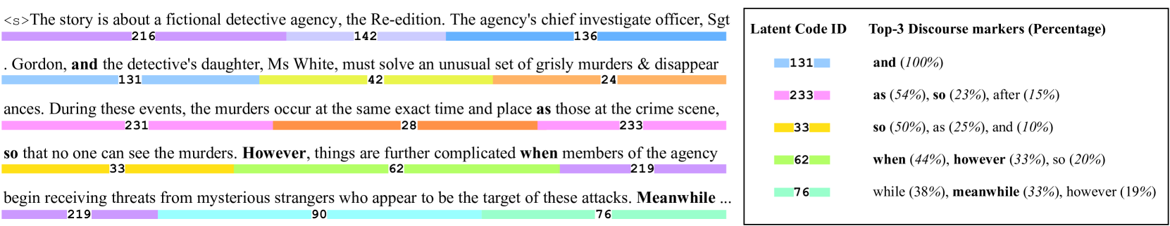
Figure 3: A generated example of DiscoDVT with correspondent latent codes intuitively assigned to text segments of 8 bpe encodings. We list the top-3 frequent discourse markers for specific latent codes that account for explicit discourse relations in the text.

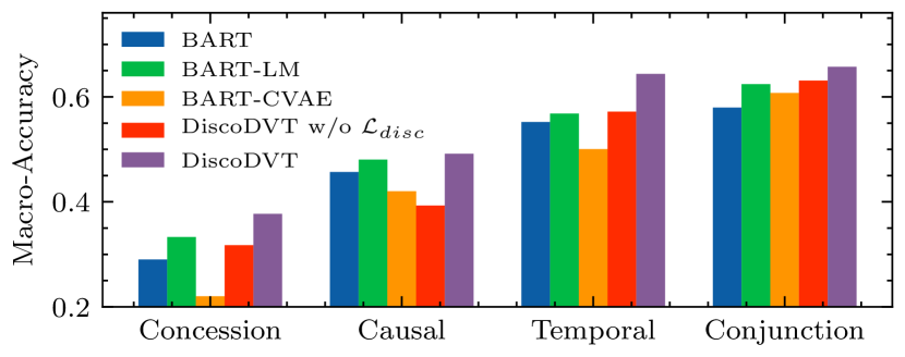
Figure 4: Macro-accuracy of classifying text pairs extracted from the passages generated by different models under the four categories of discourse relations.

4.7 Discourse-Level Evaluation

We conduct a comprehensive evaluation of the generated texts on the discourse level. To evaluate the discourse coherence, we extract text pairs connected by discourse markers from the generated texts and train a classifier to predict the relations. We then analyze the distribution of discourse relations and show that DiscoDVT uses more diverse discourse patterns as appeared in human texts.

We first fine-tune a BERT model on a dataset for discourse marker classification (Nie et al., 2019) and then train on text pairs extracted from Wikiplots to bridge the domain gap.

We manually group the discourse markers in $\mathcal{D}$ into four categories based on their most frequent senses (Prasad et al., 2008). Because of the severe class imbalance within each group, we use macro-accuracy. The results are presented in Figure 4. We show that DiscoDVT achieves higher accuracy on each category than baselines, especially on temporal relations. We also notice a minor improvement over BART-LM on causal relations since these relations are systematically harder for the model to predict (Nie et al., 2019). Finally, we show the effectiveness of discourse relation modeling by the noticeable accuracy drop when ablating $\mathcal{L}_{disc}$. We present more details and analysis in the §A.2.1.

To analyze the distribution of discourse relations, we first show the KL divergence between the distribution generated by a model and that by the human in Table 5. DiscoDVT achieves the lowest KL, indicating that the latent codes effectively learn the discourse structure of human texts. We further demonstrate that DiscoDVT can generate more diverse discourse relations in the §A.2.2.

Models	BART	BART-LM	BART-CVAE	DiscoDVT
KLD $\downarrow$	0.0308	0.0364	0.1700	0.0032

Table 5: KL divergence (KLD) between the discourse relation distribution by a model and that by the human.

4.8 Codes Study

To analyze the correspondence between discrete latent codes and texts, we present a generated example of DiscoDVT with latent codes in Figure 3. We intuitively assign each discrete latent code to the continuous bpe encodings of length 8, which match the scaling ratio of the CNN. We highlight the discourse markers in each text segment and analyze the corresponding latent code on the right. We list the top-3 frequent discourse markers for each latent code with percentage. We can see that the latent codes learn meaningful correspondence to the discourse relations that guide the model to generate coherent and logical texts. Besides, we also discover that some latent codes learn patterns indicating the beginning or ending of the story, e.g., code ID 216’s most frequent 4-gram pattern is The story is about/set/based. More generation examples of different models are provided in the §B.

5 Ethics Statement

We observe that the proposed model may sometimes generate inaccurate or fictitious contents due to the systematic biases of model pre-training on the web corpora and the open-domain characteristics of the story generation datasets. We recommend the users to carefully examine the ethical ramifications of the generated contents in the real-world applications and demonstrations.

6 Conclusion

We present DiscoDVT, a discourse-aware discrete variational Transformer for long text generation. DiscoDVT learns a discrete variable sequence that summarizes the global structure of the text, which is then applied to guide the step-wise decoding process to maintain a coherent discourse structure. We further introduce a discourse-aware objective to the discrete latent representations to model discourse relations within the text. Extensive experiments demonstrate that the DiscoDVT can generate long texts with better long-range coherence with interpretable latent codes.

Appendix A Appendices

A.1 Ablation Study on CNN Layers

Since the CNN layers are essential structures in our model for abstracting high-level features of the text, we conduct an ablation study to see the effect of varying the number of CNN layers. Figure 5 (a) plot the distribution of code utilization of the generated examples when using different number of CNN layers. The code utilization is calculated as the type number of used latent codes divided by the length of the latent codes. A high code utilization reflects a sufficient utilization of the whole information capacity of the variational bottleneck where each latent code learns more meaningful information of distinct patterns in the text (Kaiser et al., 2018).

We observe that the code utilization is maximized when using 3 CNN layers, while either increasing or decreasing the number of CNN layers leads to a decline in the code utilization. We conjecture that when using shallow CNN layers, each latent code only captures local text features and cannot learn high-level information for long text reconstruction. While when using more CNN layers, a larger receptive field for each latent code increases its modeling complexity for longer text chunks. As shown in Figure 5 (b), we present the generation performance in MSJ-2 and observe a similar tendency to the results of the average code utilization.

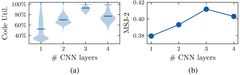
Figure 5: Results of our model with a different number of CNN layers. (a) Distribution of code utilization. (b) Generation performance in MSJ-2.

A.2 Details on Discourse-Level Evaluation

A.2.1 More Analysis on Discourse Coherence

We present fine-grained accuracies for different discourse markers under the four high-level categories in Table 6. We observe that our proposed DiscoDVT achieves the highest accuracy on six out of ten classes of discourse markers comparing to the chosen baselines. Moreover, DiscoDVT’s performance is more balanced across different discourse markers, while baseline models have low accuracy in specific types of discourse markers, e.g., BART achieves 30% accuracy on before. Finally, we show that even without the discourse-aware objective, the proposed discrete bottleneck learns to abstract some commonly used discourse relations and achieves the highest accuracy on and and also.

Model	Concession	Causal		Temporal				Conjunction
	although	because	so	before	after	as	then	and	also	still
BART	0.290	0.463	0.450	0.300	0.615	0.564	0.730	0.839	0.511	0.389
BART-LM	0.333	0.501	0.460	0.500	0.620	0.486	0.667	0.844	0.529	0.500
BART-CVAE	0.220	0.412	0.429	0.375	0.529	0.377	0.721	0.755	0.585	0.483
DiscoDVT	0.377	0.548	0.435	0.674	0.623	0.547	0.731	0.842	0.580	0.550
w/o $\mathcal{L}_{disc}$	0.317	0.361	0.425	0.458	0.612	0.549	0.667	0.846	0.612	0.434

Table 6: Fine-grained classification accuracies for different discourse markers under four high-level categories.

A.2.2 Evaluating Discourse-Level Diversity

To quantitatively understand the discourse diversity of the generated texts, we propose to assess the diversity of discourse relations in the generated texts.

We first calculate the proportion of different discourse relations and discourse markers used in the texts generated by DiscoDVT on Wikiplots and show the results in Figure 6. The model shows a diverse preference for different discourse relations that enrich the discourse structure of the generated passages.

We further compare the utilization percentage of discourse relations across different models and show the results in Table 7. DiscoDVT exhibits more discourse diversity than the other baselines indicated by a higher entropy score and resembles the golden distribution most closely. Specifically, BART and BART-CVAE mainly generate commonly used discourse markers, such as and in conjunction, while express less other complicated relations, such as temporal and causal relations. When ablating the discourse relation modeling objective, we also observe a decline in discourse diversity.

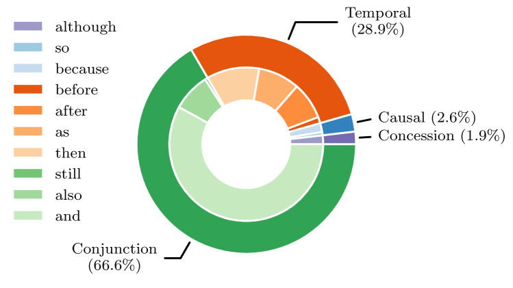
Figure 6: Percentage of different discourse markers and high-level discourse relations in the generated texts of DiscoDVT on Wikiplots.

Models	Conc.	Caus.	Temp.	Conj.	Entr. $\uparrow$
Golden	2.28%	2.56%	29.06%	66.10%	1.17
BART	0.84%	1.66%	23.37%	74.13%	0.97
BART-LM	0.56%	1.66%	24.30%	73.49%	0.96
BART-CVAE	0.20%	1.70%	14.07%	84.02%	0.73
DiscoDVT	1.86%	2.59%	28.94%	66.61%	1.15
w/o $\mathcal{L}_{\text{disc}}$	1.74%	2.10%	27.44%	68.73%	1.10

Table 7: Percentage of four categories of discourse relations, i.e., Concession, Causal, Temporal and Conjunction in the generated samples of different models and the golden references. The Entropy is calculated over these categories in bits.

A.3 Experimental Details

A.3.1 Data Preprocessing

BookCorpus: We collect a subset of 322k contiguous text segments with at least 512 bpe subwords from the BookCorpus. We reserve the first 512 subwords of each example for training.

Wikiplots: We use the official split of Wikiplots. We preserve a maximum number of 16 subwords for the input title and 512 subwords for the story, respectively.

WritingPrompts: We use the official split of WritingPrompts. We strip the accents and the newline markers. We preserve a maximum number of 64 subwords for the input prompt and 512 subwords for the story, respectively.

A.3.2 Details on Discourse Annotations Preparation

We focus on a subset of unambiguous discourse markers $\mathcal{D}$ including although, so, because, before, after, as, then, and, also and still. An instance of discourse annotation consists of a discourse connective linking a pair of arguments where the first argument (Arg1) is the main clause and the second argument (Arg2) is syntactically bound to the connective.

Prasad et al. (2008) found that 61% of discourse markers and the two arguments appear (with quite flexible order) in the same sentence, and 30% link one argument to the immediately previous sentence. Due to their high coverage, we focus on automatically extracting these two types of discourse patterns.

We resort to universal dependency grammar that provides sufficient information to extract the discourse markers and the associated two arguments. For each discourse marker of interest, we follow Nie et al. (2019) and use appropriate dependency patterns to extract intra-sentence discourse relations as shown in Figure 7. In each example, Arg1 is in italics, Arg2 is in boldface, and the discourse marker is underlined.

We first parse each sentence into a dependency tree with the Stanford CoreNLP toolkit (Manning et al., 2014). Then we identify discourse markers and the spans of Arg1 and Arg2 based on the dependency patterns and ensure that the two arguments together with the marker cover the whole sentence. If there are multiple discourse markers in one sentence, we preserve the one that divides the sentence more evenly. If the parsing results reveal that there is only one argument in the sentence that connects with the discourse marker, we heuristically label the previous adjacent sentence as Arg1 (see the next sentence pattern in Figure 7).

For each story in the dataset, we first split it into individual sentences and then apply the above steps for extraction until all the adjacent EDUs (either a complete sentence or a parsed sub-sentence) are labeled with proper relations. The label candidates are the combination of discourse markers from $\mathcal{D}$ and two possible directions that indicate how these two text spans are linked together. For example, in Figure 7 (a), the label of the text pair will be although_arg2_arg1 according to the order of the two arguments. If no discourse relation is identified from the pair of text spans, they are labeled with unknown.

Figure 7: Dependency patterns of the 10 discourse markers in $\mathcal{D}$ with annotated examples from Wikiplots. Labels above the arrows are grammatical relations defined in Manning et al. (2014).*: The next sentence pattern identifies the adjacent two sentences as Arg1 and Arg2.

A.3.3 Details on Training Settings

To improve the reproducibility of our model, we provide the detailed training settings in this section.

We implement our codes based on the repository of Huggingface’s Transformers (Wolf et al., 2020). For the posterior network, we initialize the Transformer encoder with the pre-trained parameters of the encoder of $\text{BART}_{\text{base}}$ (82M parameters). The generator model is initialized with the pre-trained checkpoint of $\text{BART}_{\text{base}}$ (140M parameters). Other randomly initialized parameters, including the CNN layers, the transposed CNN layers, the latent code embeddings, etc., sum up to 2.5M parameters. The prior network is also a Transformer encoder-decoder that uses the same architecture as $\text{BART}_{\text{base}}$ (140M parameters).

Warm-Start Training

We collect 322K contiguous texts from BookCorpus (Zhu et al., 2015) and keep the first 512 bpe subwords of each example for training. Since the warm-start training aims at initializing the latent embeddings for reconstructing the target text, we do not feed any input to the encoder. We use a fixed Gumbel temperature of 0.9 and a fixed learning rate of 1e-4. We use a batch size of 4 and a gradient accumulation step of 4 and train on the collected data for one epoch which takes about 7 hours on 1 GeForce RTX 2080 (11G).

Fine-tuning

For fine-tuning the generator and the posterior network for text reconstruction, we anneal the Gumbel temperature from $\tau_{max}=0.9$ to $\tau_{min}=0.1$ using exponential decay schedule where the Gumbel temperature $\tau$ at step $T$ is: $\max[\tau_{min},\tau_{max}\times\exp(-10^{-4}\times T)]$. We linearly decrease the learning rate from 1e-4 to 0 throughout the fine-tuning. We use a batch size of 4 and a gradient accumulation step of 4. We fine-tune for five epochs on Wikiplots and one epoch on WritingPrompts, which takes about 12 hours and 6 hours on 1 GeForce RTX 2080 (11G), respectively.

For fine-tuning the prior network, we initialize the encoder with the pre-trained parameters of the encoder of $\text{BART}_{\text{base}}$. We linearly decrease the learning rate from 1e-4 to 0 during training. The maximum target sequence length is set to $\text{MaxLength}=64$. We use a batch size of 128 and a gradient accumulation step of 8. We fine-tune the model for 100 epochs which takes about 13 hours on 1 GeForce RTX 2080 (11G). During inference, we randomly sample a sequence of latent codes from the prior network autoregressively and set the minimum sequence length to 38 and 44 for Wikiplots and WritingPrompts, respectively.

We present the hyper-parameter search space in Table 8. The number of hyper-parameter search trials was 10. We adopt a manual search to select the hyper-parameters, and the selection criterion was BLEU-1 on the validation set when fine-tuning on the downstream datasets.

Hyper-parameter	Search Space
Learning Rate	choice[8e-5, 1e-4, 2e-4]
Training Epoch	choice[1, 2, 3, 4, 5]
Batch Size	choice[4, 8, 16]
Input Length	choice[16, 32, 64]
Output Length	512
Latent Vocabulary Size	choice[32, 64, 128, 256, 512]
Top-p	choice[0.8, 0.9, 1.0]
Maximum Gradient Norm	1.0
Optimizer	AdamW
Epsilon (for AdamW)	1e-8

Table 8: Hyper-parameter search space of DiscoDVT during fine-tuning. choice indicates that the listed numbers will be chosen with the same probability.

Appendix B Generation Examples

We present the generation examples from different models on Wikiplots in Table 9. We observe that baselines including BART-LM and BART-CVAE suffer from repetition problem as the contexts grow longer while DiscoDVT maintains a better discourse structure of the text by the global discrete latent codes and stays on topic throughout the whole story (indicated by the frequent usage of the keyword “Probe 7”). Finally, we observe that existing models have potential spelling mistakes when generating complicated entities in the open-domain scenario. This phenomenon is severe in BART as in the example, which even hinders readability. We suggest that a future direction to mitigate this issue is to construct entity plots by substituting entity mentions with placeholders and apply the copy mechanism.

Title	Probe 7, Over and Out
BART	In a field hospital, dr David Mihalya discovers a corpse in a nearby car. His search leads him to a facility where his own corpse is being guarded by a secret military unit. Mihalai visits the unit and discovers that the building is a military barracks built in 1940, and that a number of the soldiers are killed in an explosion. Muhalya is taken to the military base to be interrogated, but is brought into conflict with his commanding officer, Captain James Mihalia, who also appears to be involved. Mohalya asks Mihali to give him a call as a replacement for Mihail. Mishali says that he will be sent to investigate, and he goes to see Mihanya. Muthali says they were sent to an undisclosed location when he was a child, and they are now in the same military camp. Mighali and Mihaela begin to see each other, and the two are seen to have a casual sex. Makhalya says she was "happy about her" as Mihiya said he never saw her. Mumbali is shocked at Mihmya’s response and tries to get her to get to know Mihyasa, but she rejects him.
BART-LM	In a field where men are in labor and women are selling women, a research firm is in session with an eccentric scientist who is trying to determine a cure for a blood disorder. The scientist goes to a hospital to visit the woman and discovers that her liver is growing to a dangerously high size, and she has a blood clot. The technician explains that she has to be careful not to leave the woman to go through an experimental procedure to remove the clot, but she is unable to live with the strain and her liver can’t survive without a transplant. After the procedure, the team finds that the woman’s liver has enlarged to a lethal size. However, in the process, the patient gets out of the hospital and is sent to a large hospital in the countryside where he meets with a young woman named Elizabeth. Elizabeth does not recognise Elizabeth, but Elizabeth quickly recognises Elizabeth’s condition. Elizabeth begins to suspect Elizabeth and Elizabeth’s secret relationship and believes Elizabeth to be linked to Elizabeth.
BART-CVAE	The series tells the story of Peter Smith, a boy from a small town, who fell in love, and decided to find the way to end the romance. Peter and his brother and friend, Mike, a successful lawyer, return to their town, and have the prospect of dating and marrying. After Peter discovers that Mike is with Paul, he decides to take his sister, Laura, with him and give them and his friends the word "love" and so on, until his sister says "Yes". It is up to Peter to resolve this dispute, but to reach an end with the men as good-luck, and help people in other ways. After a short visit to the church, Paul discovers that Pete and Laura are a couple, and has made a difference of how people think. He becomes concerned and asks Laura about Peter, so as to make her believe that she is, in fact, married to Peter. In order to resolve the situation, Peter uses a combination of the words "Love" and "Dollar" (for "love") in the name of a woman, but, for Peter, he can only say the words at the end and, when Peter, Laura and Peter end up in a bed in Peter’s home, as far as Peter sees, is lying on the bed. Peter thinks about what to do at the hospital, and Laura tells him to go look at Pete. Peter asks Peter about Pete and goes, and Pete mentions that David’s wife is being married with two children, but Peter says that the children can not be married, or that he isn’t with her for such a short period of time. Peter goes over to Peter’s house, and he asks Peter for a second time.
DiscoDVT	The story begins in the near future in the year 2009. An alien race called the Invaders appear and break the Galactic Federation and destroy the Cardassians from their planet. A group of mercenaries called the "Blue Angels of New Generation" are tasked with trying to destroy the Defiant. They use a device called a Probe 7 in order to kill the Invaders. The probe must send a distress signal to the Federation starship, commanded by the "Sister’s" pilot, Professor Moriarty (voiced by Arthur Fairchild from the film The Secret Intelligence Service). Professor Moriory, along with the Enterprise, arrive and successfully intercept the Invaders while the ship remains on orbit and attacks the Federation Fleet on the planet. The Blue Angels then infiltrate the fleet to set a trap for the Invaders, hoping that they will destroy the fleet. As the Blue Angels use this technology, the Red Angels of The Invaders retaliate by destroying the Enterprise before they reach the Federation fleet. The Invaders then proceed to destroy all of Earth’s radio stations and fire the Probe 7 into the "Dominic Channel". Professor Moriorthy then uses Probe 7 to gain access to his ship’s central control, which contains an orbiting outpost called the Black Mesa.

Table 9: We present the first ten sentences of the stories generated by different models. We highlight the obvious repetitions, unreasonable descriptions, and potential spelling mistakes in the generated stories. The generated keywords that match the title are presented in boldface.

References

- Bao et al. (2021) Yu Bao, Shujian Huang, Tong Xiao, Dongqi Wang, Xinyu Dai, and Jiajun Chen. 2021. Non-autoregressive translation by learning target categorical codes. CoRR, abs/2103.11405.
- Bosselut et al. (2018) Antoine Bosselut, Asli Celikyilmaz, Xiaodong He, Jianfeng Gao, Po-Sen Huang, and Yejin Choi. 2018. Discourse-aware neural rewards for coherent text generation. In Proceedings of the 2018 Conference of the North American Chapter of the Association for Computational Linguistics: Human Language Technologies, NAACL-HLT 2018, New Orleans, Louisiana, USA, June 1-6, 2018, Volume 1 (Long Papers), pages 173–184. Association for Computational Linguistics.
- Dieleman et al. (2018) Sander Dieleman, Aäron van den Oord, and Karen Simonyan. 2018. The challenge of realistic music generation: modelling raw audio at scale. In Advances in Neural Information Processing Systems 31: Annual Conference on Neural Information Processing Systems 2018, NeurIPS 2018, December 3-8, 2018, Montréal, Canada, pages 8000–8010.
- Fan et al. (2018) Angela Fan, Mike Lewis, and Yann N. Dauphin. 2018. Hierarchical neural story generation. In Proceedings of the 56th Annual Meeting of the Association for Computational Linguistics, ACL 2018, Melbourne, Australia, July 15-20, 2018, Volume 1: Long Papers, pages 889–898. Association for Computational Linguistics.
- Fan et al. (2019) Angela Fan, Mike Lewis, and Yann N. Dauphin. 2019. Strategies for structuring story generation. In Proceedings of the 57th Conference of the Association for Computational Linguistics, ACL 2019, Florence, Italy, July 28- August 2, 2019, Volume 1: Long Papers, pages 2650–2660. Association for Computational Linguistics.
- Fleiss (1971) Joseph L. Fleiss. 1971. Measuring nominal scale agreement among many raters. Psychological Bulletin, 76(5):378–382.
- Goldfarb-Tarrant et al. (2020) Seraphina Goldfarb-Tarrant, Tuhin Chakrabarty, Ralph M. Weischedel, and Nanyun Peng. 2020. Content planning for neural story generation with aristotelian rescoring. In Proceedings of the 2020 Conference on Empirical Methods in Natural Language Processing, EMNLP 2020, Online, November 16-20, 2020, pages 4319–4338. Association for Computational Linguistics.
- Guan et al. (2020) Jian Guan, Fei Huang, Minlie Huang, Zhihao Zhao, and Xiaoyan Zhu. 2020. A knowledge-enhanced pretraining model for commonsense story generation. Trans. Assoc. Comput. Linguistics, 8:93–108.
- Hobbs (1985) J. Hobbs. 1985. On the coherence and structure of discourse.
- Holtzman et al. (2020) Ari Holtzman, Jan Buys, Li Du, Maxwell Forbes, and Yejin Choi. 2020. The curious case of neural text degeneration. In 8th International Conference on Learning Representations, ICLR 2020, Addis Ababa, Ethiopia, April 26-30, 2020. OpenReview.net.
- Jang et al. (2017) Eric Jang, Shixiang Gu, and Ben Poole. 2017. Categorical reparameterization with gumbel-softmax. In 5th International Conference on Learning Representations, ICLR 2017, Toulon, France, April 24-26, 2017, Conference Track Proceedings. OpenReview.net.
- Jurafsky and Martin (2000) Daniel Jurafsky and James H. Martin. 2000. Speech and language processing - an introduction to natural language processing, computational linguistics, and speech recognition. Prentice Hall series in artificial intelligence. Prentice Hall.
- Kaiser et al. (2018) Lukasz Kaiser, Samy Bengio, Aurko Roy, Ashish Vaswani, Niki Parmar, Jakob Uszkoreit, and Noam Shazeer. 2018. Fast decoding in sequence models using discrete latent variables. In Proceedings of the 35th International Conference on Machine Learning, ICML 2018, Stockholmsmässan, Stockholm, Sweden, July 10-15, 2018, volume 80 of Proceedings of Machine Learning Research, pages 2395–2404. PMLR.
- Kingma and Welling (2014) Diederik P. Kingma and Max Welling. 2014. Auto-encoding variational bayes. In 2nd International Conference on Learning Representations, ICLR 2014, Banff, AB, Canada, April 14-16, 2014, Conference Track Proceedings.
- Kingma et al. (2016) Durk P Kingma, Tim Salimans, Rafal Jozefowicz, Xi Chen, Ilya Sutskever, and Max Welling. 2016. Improved variational inference with inverse autoregressive flow. In Advances in Neural Information Processing Systems, volume 29. Curran Associates, Inc.
- Ko and Li (2020) Wei-Jen Ko and Junyi Jessy Li. 2020. Assessing discourse relations in language generation from GPT-2. In Proceedings of the 13th International Conference on Natural Language Generation, pages 52–59, Dublin, Ireland. Association for Computational Linguistics.
- Lewis et al. (2020) Mike Lewis, Yinhan Liu, Naman Goyal, Marjan Ghazvininejad, Abdelrahman Mohamed, Omer Levy, Veselin Stoyanov, and Luke Zettlemoyer. 2020. BART: denoising sequence-to-sequence pre-training for natural language generation, translation, and comprehension. In Proceedings of the 58th Annual Meeting of the Association for Computational Linguistics, ACL 2020, Online, July 5-10, 2020, pages 7871–7880. Association for Computational Linguistics.
- Li et al. (2020) Chunyuan Li, Xiang Gao, Yuan Li, Baolin Peng, Xiujun Li, Yizhe Zhang, and Jianfeng Gao. 2020. Optimus: Organizing sentences via pre-trained modeling of a latent space. In Proceedings of the 2020 Conference on Empirical Methods in Natural Language Processing, EMNLP 2020, Online, November 16-20, 2020, pages 4678–4699. Association for Computational Linguistics.
- Li et al. (2016) Jiwei Li, Michel Galley, Chris Brockett, Jianfeng Gao, and Bill Dolan. 2016. A diversity-promoting objective function for neural conversation models. In NAACL HLT 2016, The 2016 Conference of the North American Chapter of the Association for Computational Linguistics: Human Language Technologies, San Diego California, USA, June 12-17, 2016, pages 110–119. The Association for Computational Linguistics.
- Li et al. (2015) Jiwei Li, Minh-Thang Luong, and Dan Jurafsky. 2015. A hierarchical neural autoencoder for paragraphs and documents. In Proceedings of the 53rd Annual Meeting of the Association for Computational Linguistics and the 7th International Joint Conference on Natural Language Processing of the Asian Federation of Natural Language Processing, ACL 2015, July 26-31, 2015, Beijing, China, Volume 1: Long Papers, pages 1106–1115. The Association for Computer Linguistics.
- Loshchilov and Hutter (2019) Ilya Loshchilov and Frank Hutter. 2019. Decoupled weight decay regularization. In 7th International Conference on Learning Representations, ICLR 2019, New Orleans, LA, USA, May 6-9, 2019. OpenReview.net.
- Maddison et al. (2017) Chris J. Maddison, Andriy Mnih, and Yee Whye Teh. 2017. The concrete distribution: A continuous relaxation of discrete random variables. In 5th International Conference on Learning Representations, ICLR 2017, Toulon, France, April 24-26, 2017, Conference Track Proceedings. OpenReview.net.
- Manning et al. (2014) Christopher D. Manning, Mihai Surdeanu, John Bauer, Jenny Finkel, Steven J. Bethard, and David McClosky. 2014. The Stanford CoreNLP natural language processing toolkit. In Association for Computational Linguistics (ACL) System Demonstrations, pages 55–60.
- Montahaei et al. (2019) Ehsan Montahaei, Danial Alihosseini, and Mahdieh Soleymani Baghshah. 2019. Jointly measuring diversity and quality in text generation models. CoRR, abs/1904.03971.
- Nie et al. (2019) Allen Nie, Erin Bennett, and Noah D. Goodman. 2019. Dissent: Learning sentence representations from explicit discourse relations. In Proceedings of the 57th Conference of the Association for Computational Linguistics, ACL 2019, Florence, Italy, July 28- August 2, 2019, Volume 1: Long Papers, pages 4497–4510. Association for Computational Linguistics.
- Papineni et al. (2002) Kishore Papineni, Salim Roukos, Todd Ward, and Wei-Jing Zhu. 2002. Bleu: a method for automatic evaluation of machine translation. In Proceedings of the 40th Annual Meeting of the Association for Computational Linguistics, July 6-12, 2002, Philadelphia, PA, USA, pages 311–318. ACL.
- Prasad et al. (2008) Rashmi Prasad, Nikhil Dinesh, Alan Lee, Eleni Miltsakaki, Livio Robaldo, Aravind Joshi, and Bonnie Webber. 2008. The Penn Discourse TreeBank 2.0. In Proceedings of the Sixth International Conference on Language Resources and Evaluation (LREC’08), Marrakech, Morocco. European Language Resources Association (ELRA).
- Radford et al. (2019) Alec Radford, Jeffrey Wu, Rewon Child, David Luan, Dario Amodei, and Ilya Sutskever. 2019. Language models are unsupervised multitask learners. OpenAI blog, 1(8):9.
- Razavi et al. (2019) Ali Razavi, Aäron van den Oord, and Oriol Vinyals. 2019. Generating diverse high-fidelity images with VQ-VAE-2. In Advances in Neural Information Processing Systems 32: Annual Conference on Neural Information Processing Systems 2019, NeurIPS 2019, December 8-14, 2019, Vancouver, BC, Canada, pages 14837–14847.
- Rolfe (2017) Jason Tyler Rolfe. 2017. Discrete variational autoencoders. In 5th International Conference on Learning Representations, ICLR 2017, Toulon, France, April 24-26, 2017, Conference Track Proceedings. OpenReview.net.
- See et al. (2019) Abigail See, Aneesh Pappu, Rohun Saxena, Akhila Yerukola, and Christopher D. Manning. 2019. Do massively pretrained language models make better storytellers? In Proceedings of the 23rd Conference on Computational Natural Language Learning, CoNLL 2019, Hong Kong, China, November 3-4, 2019, pages 843–861. Association for Computational Linguistics.
- Serban et al. (2017) Iulian Vlad Serban, Alessandro Sordoni, Ryan Lowe, Laurent Charlin, Joelle Pineau, Aaron C. Courville, and Yoshua Bengio. 2017. A hierarchical latent variable encoder-decoder model for generating dialogues. In Proceedings of the Thirty-First AAAI Conference on Artificial Intelligence, February 4-9, 2017, San Francisco, California, USA, pages 3295–3301. AAAI Press.
- Shao et al. (2019) Zhihong Shao, Minlie Huang, Jiangtao Wen, Wenfei Xu, and Xiaoyan Zhu. 2019. Long and diverse text generation with planning-based hierarchical variational model. In Proceedings of the 2019 Conference on Empirical Methods in Natural Language Processing and the 9th International Joint Conference on Natural Language Processing, EMNLP-IJCNLP 2019, Hong Kong, China, November 3-7, 2019, pages 3255–3266. Association for Computational Linguistics.
- Shen et al. (2019) Dinghan Shen, Asli Celikyilmaz, Yizhe Zhang, Liqun Chen, Xin Wang, Jianfeng Gao, and Lawrence Carin. 2019. Towards generating long and coherent text with multi-level latent variable models. In Proceedings of the 57th Conference of the Association for Computational Linguistics, ACL 2019, Florence, Italy, July 28- August 2, 2019, Volume 1: Long Papers, pages 2079–2089. Association for Computational Linguistics.
- Shi et al. (2018) Zhan Shi, Xinchi Chen, Xipeng Qiu, and Xuanjing Huang. 2018. Toward diverse text generation with inverse reinforcement learning. In Proceedings of the Twenty-Seventh International Joint Conference on Artificial Intelligence, IJCAI 2018, July 13-19, 2018, Stockholm, Sweden, pages 4361–4367. ijcai.org.
- Tan et al. (2020) Bowen Tan, Zichao Yang, Maruan Al-Shedivat, Eric P. Xing, and Zhiting Hu. 2020. Progressive generation of long text. CoRR, abs/2006.15720.
- van den Oord et al. (2017) Aäron van den Oord, Oriol Vinyals, and Koray Kavukcuoglu. 2017. Neural discrete representation learning. In Advances in Neural Information Processing Systems 30: Annual Conference on Neural Information Processing Systems 2017, December 4-9, 2017, Long Beach, CA, USA, pages 6306–6315.
- Welleck et al. (2020) Sean Welleck, Ilia Kulikov, Stephen Roller, Emily Dinan, Kyunghyun Cho, and Jason Weston. 2020. Neural text generation with unlikelihood training. In 8th International Conference on Learning Representations, ICLR 2020, Addis Ababa, Ethiopia, April 26-30, 2020. OpenReview.net.
- Wiseman et al. (2018) Sam Wiseman, Stuart M. Shieber, and Alexander M. Rush. 2018. Learning neural templates for text generation. In Proceedings of the 2018 Conference on Empirical Methods in Natural Language Processing, Brussels, Belgium, October 31 - November 4, 2018, pages 3174–3187. Association for Computational Linguistics.
- Wolf et al. (2020) Thomas Wolf, Lysandre Debut, Victor Sanh, Julien Chaumond, Clement Delangue, Anthony Moi, Pierric Cistac, Tim Rault, Rémi Louf, Morgan Funtowicz, Joe Davison, Sam Shleifer, Patrick von Platen, Clara Ma, Yacine Jernite, Julien Plu, Canwen Xu, Teven Le Scao, Sylvain Gugger, Mariama Drame, Quentin Lhoest, and Alexander M. Rush. 2020. Transformers: State-of-the-art natural language processing. In Proceedings of the 2020 Conference on Empirical Methods in Natural Language Processing: System Demonstrations, pages 38–45, Online. Association for Computational Linguistics.
- Xu et al. (2020) Peng Xu, Mostofa Patwary, Mohammad Shoeybi, Raul Puri, Pascale Fung, Anima Anandkumar, and Bryan Catanzaro. 2020. MEGATRON-CNTRL: controllable story generation with external knowledge using large-scale language models. In Proceedings of the 2020 Conference on Empirical Methods in Natural Language Processing, EMNLP 2020, Online, November 16-20, 2020, pages 2831–2845. Association for Computational Linguistics.
- Yao et al. (2019) Lili Yao, Nanyun Peng, Ralph M. Weischedel, Kevin Knight, Dongyan Zhao, and Rui Yan. 2019. Plan-and-write: Towards better automatic storytelling. In The Thirty-Third AAAI Conference on Artificial Intelligence, AAAI 2019, The Thirty-First Innovative Applications of Artificial Intelligence Conference, IAAI 2019, The Ninth AAAI Symposium on Educational Advances in Artificial Intelligence, EAAI 2019, Honolulu, Hawaii, USA, January 27 - February 1, 2019, pages 7378–7385. AAAI Press.
- Zhao et al. (2018) Tiancheng Zhao, Kyusong Lee, and Maxine Eskénazi. 2018. Unsupervised discrete sentence representation learning for interpretable neural dialog generation. In Proceedings of the 56th Annual Meeting of the Association for Computational Linguistics, ACL 2018, Melbourne, Australia, July 15-20, 2018, Volume 1: Long Papers, pages 1098–1107. Association for Computational Linguistics.
- Zhao et al. (2017) Tiancheng Zhao, Ran Zhao, and Maxine Eskénazi. 2017. Learning discourse-level diversity for neural dialog models using conditional variational autoencoders. In Proceedings of the 55th Annual Meeting of the Association for Computational Linguistics, ACL 2017, Vancouver, Canada, July 30 - August 4, Volume 1: Long Papers, pages 654–664. Association for Computational Linguistics.
- Zhu et al. (2015) Yukun Zhu, Ryan Kiros, Richard S. Zemel, Ruslan Salakhutdinov, Raquel Urtasun, Antonio Torralba, and Sanja Fidler. 2015. Aligning books and movies: Towards story-like visual explanations by watching movies and reading books. In 2015 IEEE International Conference on Computer Vision, ICCV 2015, Santiago, Chile, December 7-13, 2015, pages 19–27. IEEE Computer Society.