Doubly-Trained Adversarial Data Augmentation
for Neural Machine Translation

Abstract

Neural Machine Translation (NMT) models are known to suffer from noisy inputs. To make models robust, we generate adversarial augmentation samples that attack the model and preserve the source-side semantic meaning at the same time. To generate such samples, we propose a doubly-trained architecture that pairs two NMT models of opposite translation directions with a joint loss function, which combines the target-side attack and the source-side semantic similarity constraint. The results from our experiments across three different language pairs and two evaluation metrics show that these adversarial samples improve the model robustness.

1 Introduction

When NMT models are trained on clean parallel data, they are not exposed to much noise, resulting in poor robustness when translating noisy input texts. Various adversarial attack methods have been explored for computer vision Yuan et al. (2018), including Fast Gradient Sign Methods Goodfellow et al. (2015), and generative adversarial networks (GAN; Goodfellow et al., 2014), among others. Most of these methods are white-box attacks where model parameters are accessible during the attack so that the attack is much more effective. Good adversarial samples could also enhance model robustness by introducing perturbation as data augmentation Goodfellow et al. (2014); Chen et al. (2020).

Due to the discrete nature of natural languages, most of the early-stage adversarial attacks on NMT focused on black-box attacks (attacks without access to model parameters) and use techniques such as string modification based on edit distance Karpukhin et al. (2019) or random changes of words in input sentence Ebrahimi et al. (2018)). Such black-box methods can improve model robustness. However, model parameters are not accessible in black-box attacks and therefore restrict black-box methods’ capacity. There is also work that tried to incorporate gradient-based adversarial techniques into natural languages processing, such as virtual training algorithm Miyato et al. (2017) and adversarial regularization Sato et al. (2019). These gradient-based adversarial approaches, to some extent, improve model performance and robustness. Cheng et al. (2019, 2020) further constrained the direction of perturbation with source-side semantic similarity and observed better performance.

Our work improves the gradient-based generation mechanism with a doubly-trained system, inspired by dual learning Xia et al. (2016). The doubly-trained system consists of a forward (translate from source language to target language) and a backward (translate target language to source language) model. After pretraining both forward and backward models, our augmentation process has three steps:

1. Attack Step: Train forward and backward models at the same time to update the shared embedding of source language (embedding of the forward model’s encoder and the backward model’s decoder).

2. Perturbation Step: Generate adversarial sequences by modifying source input sentences with random deletion and nearest neighbor search.

3. Augmentation Training Step: Train the forward model on the adversarial data.

We applied our method on test data with synthetic noise and compared it against different baseline models. Experiments across three languages showed consistent improvement of model robustness using our algorithm.

2 Background

Neural Machine Translation

Given a parallel corpus $S={({\boldsymbol{\mathbf{x}}}^{(s)},{\boldsymbol{\mathbf{y}}}^{(s)})}_{s=1}^{|S|}$, for each pair of sentences, the model will compute the translation probability:

$$P({\boldsymbol{\mathbf{y}}}|{\boldsymbol{\mathbf{x}}};\theta)=\prod_{n=1}^{N}P({\boldsymbol{\mathbf{y}}}_{n}|{\boldsymbol{\mathbf{x}}},{\boldsymbol{\mathbf{y}}}_{<n};\theta)$$

where $\theta$ is a set of model parameters and ${\boldsymbol{\mathbf{y}}}_{<n}={\boldsymbol{\mathbf{y}}}_{1},\cdots,{\boldsymbol{\mathbf{y}}}_{n}$ is a partial translation until $n^{th}$ position. The training objective is to maximize the log-likelihood of $S$, or equivalently, minimizing the negative log-likelihood loss (NLL):

$$\mathcal{L}_{\text{NLL}}(\theta) =-\sum_{s=1}^{S}\log P({\boldsymbol{\mathbf{y}}}^{(s)}|{\boldsymbol{\mathbf{x}}}^{(s)};\theta)$$ (1)

$$=-\sum_{s=1}^{S}\sum_{n=1}^{N(s)}\sum_{e}^{V}y^{(s)}_{n,e}\log\hat{y}^{(s)}_{n,e}$$

$$\hat{\theta}_{\text{NLL}} =\underset{\theta}{\text{argmin}}\{\mathcal{L}_{\text{NLL}}(\theta)\}$$

Where $N(s)$ is length of $y^{(s)}$, $V$ is the vocabulary, $y^{(s)}_{n,e}=1$ if the $n^{th}$ word in $y^{(s)}$ is $e$ and $\hat{y}^{(s)}_{n,e}$ is the predicted probability of word entry e as the $n^{th}$ word for $y^{(s)}$. To train the NMT model, we compute the partial of the loss over model parameter $\frac{\partial\mathcal{L}_{\text{NLL}}(\theta)}{\partial\theta}$ to update $\theta$. Note that sometimes we use NLL and cross entropy interchangeably because the last layer of our model is always softmax.

Minimum Risk Training (MRT)

Shen et al. (2016) introduces evaluation metric into loss function and assume that the optimal set of model parameters will minimize the expected loss on the training data. The loss function is defined as $\Delta({\boldsymbol{\mathbf{y}}},{\boldsymbol{\mathbf{y}}}^{(s)})$ to measure the discrepancy between model output y and gold standard translation ${\boldsymbol{\mathbf{y}}}^{(s)}$. It can be any negative sentence-level evaluation metric such as BLEU, METEOR, COMET, BERTScore, (Papineni et al., 2002; Banerjee and Lavie, 2005; Rei et al., 2020; Zhang et al., 2020) etc. The risk (training objective) for the system is:

$$\mathcal{L}_{\text{MRT}} =\sum_{s=1}^{S}\mathbb{E}_{{\boldsymbol{\mathbf{y}}}|{\boldsymbol{\mathbf{x}}}^{(s)};\theta}\left[\Delta({\boldsymbol{\mathbf{y}}},{\boldsymbol{\mathbf{y}}}^{(s)})\right]$$ (2)

$$=\sum_{s=1}^{S}\sum_{{\boldsymbol{\mathbf{y}}}\in C({\boldsymbol{\mathbf{x}}})}P({\boldsymbol{\mathbf{y}}}|{\boldsymbol{\mathbf{x}}}^{(s)};\theta)\Delta({\boldsymbol{\mathbf{y}}},{\boldsymbol{\mathbf{y}}}^{(s)})$$

$$\hat{\theta}_{\text{MRT}} =\underset{\theta}{\text{argmin}}\{\mathcal{L}_{\text{MRT}}(\theta)\}$$

where $C({\boldsymbol{\mathbf{x}}}^{(s)})$ is the set of all possible candidate translation by the system. Shen et al. (2016) shows that partial of risk $\mathcal{L}_{MRT}(\theta)$ with respect to a model parameter $\theta_{i}$ does not need to differentiate $\Delta({\boldsymbol{\mathbf{y}}},{\boldsymbol{\mathbf{y}}}^{(s)})$:

$$\begin{split}\frac{\partial\mathcal{L}_{\text{MRT}}(\theta)}{\partial\theta_{i}}=\sum_{s=1}^{S}\mathbb{E}_{{\boldsymbol{\mathbf{y}}}|{\boldsymbol{\mathbf{x}}}^{(s)};\theta}\biggl{[}\Delta({\boldsymbol{\mathbf{y}}},{\boldsymbol{\mathbf{y}}}^{(s)})\times\\ \sum_{n=1}^{N^{(s)}}\frac{\partial P({\boldsymbol{\mathbf{y}}}_{n}^{(s)}|{\boldsymbol{\mathbf{x}}}^{(s)},{\boldsymbol{\mathbf{y}}}_{<n}^{(s)};\theta)/\partial\theta_{i}}{P({\boldsymbol{\mathbf{y}}}_{n}^{(s)}|{\boldsymbol{\mathbf{x}}}^{(s)},{\boldsymbol{\mathbf{y}}}_{<n}^{(s)};\theta)}\biggr{]}\end{split}$$ (3)

Hence MRT allows an arbitrary scoring function $\Delta$ to be used, whether it is differentiable or not. In our experiments, we use MRT with two metrics, BLEU Papineni et al. (2002)—the standard in machine translation and COMET Rei et al. (2020)—a newly proposed neural-based evaluation metric that correlates better with human judgement.

Adversarial Attack

Adversarial attacks generate samples that closely match input while dramatically distorting the model output. The samples can be generated by either a white-box or a black-box model. Black-box methods do not have access to the model while white-box methods have such access. A set of adversarial samples are generated by:

$$\{{\boldsymbol{\mathbf{x}}}^{\prime}|\mathcal{R}({\boldsymbol{\mathbf{x}}}^{\prime},{\boldsymbol{\mathbf{x}}})\leq\epsilon,\underset{{\boldsymbol{\mathbf{x}}}^{\prime}}{\text{argmax}}J({\boldsymbol{\mathbf{x}}}^{\prime},{\boldsymbol{\mathbf{y}}};\theta)\}$$ (4)

where $J(\cdot)$ is the probability of a sample being adversarial and $\mathcal{R}({\boldsymbol{\mathbf{x}}}^{\prime},{\boldsymbol{\mathbf{x}}})$ computes the degree of imperceptibility of perturbation ${\boldsymbol{\mathbf{x}}}^{\prime}$ compared to original input ${\boldsymbol{\mathbf{x}}}$. The smaller the $\epsilon$, the less noticeable the perturbation is. In our system, $J(\cdot)$ not only focuses on attacking the forward model, but also uses the backward model to constrain the direction of gradient update and maintain source-side semantic similarity.

3 Approach: Doubly Trained NMT for Adversarial Sample Generation

We aim to to generate adversarial samples that both preserve input’s semantic meaning and decrease the performance of a NMT model. We propose a doubly-trained system that involves two models of opposite translation direction (denote the forward model as $\theta_{st}$ and the backward model as $\theta_{ts}$). Our algorithm will train and update $\theta_{st},\theta_{ts}$ simultaneously. Note that both models are pretrained before they are used for adversarial augmentation so that they can already produce good translations. Our algorithm has three steps as shown in Figure 1.

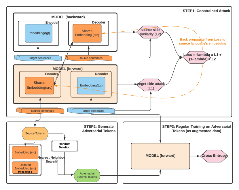
Figure 1: Visual explanation of our adversarial augmentation algorithm. Step 1: Forward and backward models are trained simultaneously and attacked by the combined objective function. (The shared embedding is modified). Step 2: input source tokens are randomly deleted or replaced by nearest neighbor search to generate adversarial samples. Step 3: forward model is trained on adversarial samples.

Step 1 – Constrained Attack to Update Embedding

The first step is to attack the system and update the source embedding. We train the models with Negative Log-Likelihood (NLL) or MRT and combine the loss from two models as our final loss function to update the shared embedding. We denote the loss for $\theta_{st}$ as $\mathcal{L}_{1}$ and loss for $\theta_{ts}$ as $\mathcal{L}_{2}$. Because we want to attack the forward model and preserve translation quality for the backward model, we make our final loss

$$\mathcal{L}=-\lambda\mathcal{L}_{1}+(1-\lambda)\mathcal{L}_{2}$$

where $\lambda\in[0,1]$ and is used as the weight to decide whether we focus on punishing the forward model (large $\lambda$) or preserving the backward model (small $\lambda$). When we use NLL as training objective, we have $\mathcal{L}_{1}=\textbf{NLL}({\boldsymbol{\mathbf{x}}}^{(s)},{\boldsymbol{\mathbf{y}}}^{(s)},\theta_{st})$ where ${\boldsymbol{\mathbf{x}}}^{(s)}$ is the input sentences, ${\boldsymbol{\mathbf{y}}}^{(s)}$ is the gold standard translation and NLL($\cdot$) is the Negative Log-Likelihood function that computes a loss based on training data ${\boldsymbol{\mathbf{x}}}^{(s)},{\boldsymbol{\mathbf{y}}}^{(s)}$ and model parameter $\theta_{st}$. Similarly we have $\mathcal{L}_{2}=\textbf{NLL}({\boldsymbol{\mathbf{y}}}^{(s)},{\boldsymbol{\mathbf{x}}}^{(s)},\theta_{ts})$

We also experimented with MRT in our doubly-trained system because we wonder if taking sentence-level scoring functions like BLEU or COMET would help improve adversarial samples’ quality. For model $\theta_{st}$, we feed in source sentences ${\boldsymbol{\mathbf{x}}}^{(s)}$ and we infer a set of possible translation $S({\boldsymbol{\mathbf{x}}}^{(s)})$ as the subset of full sample space. The loss (risk) of our prediction is therefore calculated as:

$$\mathcal{L}_{1} =\sum_{s=1}^{S}\mathbb{E}_{{\boldsymbol{\mathbf{y}}}|{\boldsymbol{\mathbf{x}}}^{(s)};\theta_{st}}\left[\Delta({\boldsymbol{\mathbf{y}}},{\boldsymbol{\mathbf{y}}}^{(s)})\right]$$ (5)

$$=\sum_{s=1}^{S}\sum_{{\boldsymbol{\mathbf{y}}}\in S({\boldsymbol{\mathbf{x}}}^{(s)})}Q({\boldsymbol{\mathbf{y}}}|{\boldsymbol{\mathbf{x}}}^{(s)};\theta_{st},\alpha)\Delta({\boldsymbol{\mathbf{y}}},{\boldsymbol{\mathbf{y}}}^{(s)})$$

where

$$Q({\boldsymbol{\mathbf{y}}}|{\boldsymbol{\mathbf{x}}}^{(s)};\theta_{st},\alpha)=\frac{P({\boldsymbol{\mathbf{y}}}|{\boldsymbol{\mathbf{x}}}^{(s)};\theta_{st})^{\alpha}}{\sum_{{\boldsymbol{\mathbf{y}}}^{\prime}\in S({\boldsymbol{\mathbf{x}}}^{(s)}})P({\boldsymbol{\mathbf{y}}}^{\prime}|{\boldsymbol{\mathbf{x}}}^{(s)};\theta_{st})^{\alpha}}$$

The value $\alpha$ here controls the sharpness of the formula and we follow Shen et al. (2016) to use $\alpha=5e^{-3}$ throughout our experiments. To sample the subset of full inference space $S({\boldsymbol{\mathbf{x}}}^{(s)})$, we use Sampling Algorithm (Shen et al., 2016) to generate k translation candidates for each input sentence (During inference time, the model outputs a probabilistic distribution over the vocabulary for each token and we sample a token based on this distribution). It is denoted as $\textbf{Sample}({\boldsymbol{\mathbf{x}}}^{(s)},\theta,k)$ in our Algorithm 1. Similarly, for model $\theta_{ts}$, we feed in the reference sentences of our parallel data and generate a set of possible translation $S({\boldsymbol{\mathbf{y}}}^{(s)})$ in source language. We compute the loss (risk) of source-side similarity as:

$$\mathcal{L}_{2} =\sum_{s=1}^{S}\mathbb{E}_{{\boldsymbol{\mathbf{x}}}|{\boldsymbol{\mathbf{y}}}^{(s)};\theta_{ts}}\left[\Delta({\boldsymbol{\mathbf{x}}},{\boldsymbol{\mathbf{x}}}^{(s)})\right]$$ (6)

$$=\sum_{s=1}^{S}\sum_{{\boldsymbol{\mathbf{x}}}\in S({\boldsymbol{\mathbf{y}}}^{(s)})}Q({\boldsymbol{\mathbf{x}}}|{\boldsymbol{\mathbf{y}}}^{(s)};\theta_{ts},\alpha)\Delta({\boldsymbol{\mathbf{x}}},{\boldsymbol{\mathbf{x}}}^{(s)})$$

After computing loss using MRT or NLL, we have

$$\mathcal{L}(\theta_{st},\theta_{ts})=-\lambda\mathcal{L}_{1}+(1-\lambda)\mathcal{L}_{2}$$

and we train the system to find

$$\hat{\theta}_{st},\hat{\theta}_{ts}=\underset{\theta_{st},\theta_{ts}}{\text{argmin}}\{\mathcal{L}(\theta_{st},\theta_{ts})\}$$

To be updated from both risks, two models need to share some parameters since $\mathcal{L}_{1}$ only affects $\theta_{st}$ and $\mathcal{L}_{2}$ only updates $\theta_{ts}$. Because word embedding is a representation of input tokens, we make it such that the source-side embedding of $\theta_{st}$ and the target-side embedding of $\theta_{ts}$ is one shared embedding. We do so because they are both representations of source language in our translation and we can use it to generate adversarial tokens for source sentences in step 2. We also freeze all other layers in two models. Thus, when we update the model parameter $\theta_{st},\theta_{ts}$, we only update the shared embedding of source language. The process described above is summarized in Algorithm 1.

Step 2 – Perturb input sentences to generate adversarial tokens

After updating the shared embedding, we can use the updated embedding to generate adversarial tokens. We introduce two kinds of noise into input sentences to generate adversarial samples: random deletion and simple replacement. Random deletion is introduced by randomly deleting some tokens in the input sentences while simple replacement is introduced by using nearest neighbor search with original and updated embedding. Our implementation is described in Section 4.3.1.

Step 3 – Train on adversarial Samples

After generating adversarial tokens from step 2, we directly train the forward model on them with the NLL loss function.

Algorithm 1 Update model embedding

  Input: Pretrained Models $\theta_{st}$ and $\theta_{ts}$, Max Number of Epochs E, Sample Size K, Sentence-Level Scoring Metric M

  Output: Updated Models $\theta_{st}$ and $\theta_{ts}$ (only the shared embedding is updated)

  while $\theta_{st}$, $\theta_{ts}$ not Converged and $e\leq E$ do

     for $({\boldsymbol{\mathbf{x}}}^{(i)},{\boldsymbol{\mathbf{y}}}^{(i)}),1<i\leq S$ do

        if using MRT as objective then

           /* sample and compute the risk */

           $S({\boldsymbol{\mathbf{x}}}^{(i)})=\textbf{Sample}({\boldsymbol{\mathbf{x}}}^{(i)},\theta_{st},K)$

           $\mathcal{L}_{1}\leftarrow\textbf{MRT}(S({\boldsymbol{\mathbf{x}}}^{(i)}),M,{\boldsymbol{\mathbf{y}}}^{(i)})$

           /* Repeat for another direction */

           $S({\boldsymbol{\mathbf{y}}}^{(i)})=\textbf{Sample}({\boldsymbol{\mathbf{y}}}^{(i)},\theta_{ts},K)$

           $\mathcal{L}_{2}\leftarrow\textbf{MRT}(S({\boldsymbol{\mathbf{y}}}^{(i)}),M,{\boldsymbol{\mathbf{x}}}^{(i)})$

        else if using NLL as objective then

           $\mathcal{L}_{1}\leftarrow\textbf{NLL}({\boldsymbol{\mathbf{x}}}^{(i)},{\boldsymbol{\mathbf{y}}}^{(i)},\theta_{st})$

           $\mathcal{L}_{2}\leftarrow\textbf{NLL}({\boldsymbol{\mathbf{x}}}^{(i)},{\boldsymbol{\mathbf{y}}}^{(i)},\theta_{ts})$

        end if

        $\mathcal{L}(\theta_{st},\theta_{ts})=-\lambda\mathcal{L}_{1}+(1-\lambda)\mathcal{L}_{2}$

        $\theta_{st},\theta_{ts}\leftarrow\nabla_{Emb}\mathcal{L}(\theta_{st},\theta_{ts})$

     end for

  end while

4 Experiment

4.1 Pretrained Model Setup

We pretrain the standard Transformer Vaswani et al. (2017) base model implemented in fairseq Ott et al. (2019). The hyper-parameters follow the transformer-en-de setup from fairseq and our script is shown in Appendix, Figure 2. We experimented on three different language pairs: Chinese-English (zh-en), German-English (de-en), and French-English (fr-en). For each language pair, two models are pretrained on the same training data using the same hyper-parameters and they share the embedding of source language. For example, for Chinese-English, we first train the forward model (zh-en) from scratch. Then we freeze the source language (zh)’s embedding from forward model and use it to pretrain our backward model (en-zh). The training data used for three languages pairs are:

1. zh-en: WMT17 Bojar et al. (2017) parallel corpus (except UN) for training, WMT2017 and 2018 newstest data for validation, and WMT2020 newstest for evaluation.

2. de-en: WMT17 parallel corpus for training, WMT2017 and 2018 newstest data for validation, and WMT2014 newstest for evaluation.

3. fr-en: WMT14 Bojar et al. (2014) parallel corpus (except UN) for training, WMT2015 newdicussdev and newsdiscusstest for validation, and WMT2014 newstest for evaluation.

For Chinese-English parallel corpus, we used a sentencepiece model of size 20k to perform BPE. For German-English and French-English data, we followed preprocessing scripts on fairseq and used subword-nmt of size 40k to perform BPE. We need two validation sets because in our experiment, we fine-tune the model with our adversarial augmentation algorithm on one of the validation set and use the other for model selection. After pretraining stage, the transformer models’ performances on test sets are shown in Table 1. The evaluation of BLEU score is computed by SacreBLEU Post (2018).

lang	BLEU	lang	BLEU	lang	BLEU
zh-en	22.8	de-en	30.2	fr-en	34.5
en-zh	36.0	en-de	24.9	en-fr	35.3

Table 1: Pretrained baseline models’ BLEU score

4.2 Doubly Trained System for Adversarial Attack

Our adversarial augmentation algorithm has three steps: the first step is performing a constrained adversarial attack while the remaining steps generate and train models on augmentation data. In this section, we experiment with only the first step and test if Algorithm 1 can generate meaning-preserving update on the embedding. Our objective function $\mathcal{L}(\theta_{st},\theta_{ts})=-\lambda\mathcal{L}_{1}+(1-\lambda)\mathcal{L}_{2}$ is a combination of two rewards from forward and backward models. The expectation is that after the perturbation on the embedding, the forward model’s performance would drastically decrease (because it’s attacked) and the backward model should still translate reasonably well (because the objective function preserves the source-side semantic meaning). We perform the experiment on Chinese-English and results are shown in Table 2. We find that models corroborate to our expectation: After 15 epochs, the forward (zh-en) model’s performance drops significantly while the backward (en-zh) model’s performance barely decreases. After 20 epochs, the forward model is producing garbage translation while the backward model is still performing well.

#Epochs	BLEU (zh-en)	BLEU (en-zh)
10	20.1	34.0
15	10.9	32.4
20	0.3	33.5
30	0.0	32.1

Table 2: Forward and backward models’ performance (of Chinese and English) after adversarial attack using MRT as training objective, described in Algorithm 1.

4.3 Doubly Trained System for Data Augmentation

From Section 4.2, we have verified that the first step of our adversarial augmentation training is effective to generate meaning-preserving perturbation on the word embedding. We then perform all three steps of our algorithm to investigate whether it is effective as an augmentation technique, which is the focus of this work. In the following subsections, we show, in detail, how the adversarial samples and noisy test data are generated, as well as the test results of our models.

Model (ZH-EN)	RD10	RD15	RD20	RD25	RD30	RP10	RP15	RP20	RP25	RP30
Baseline	25$\%$	36$\%$	46$\%$	55$\%$	63$\%$	8$\%$	14$\%$	19$\%$	22$\%$	25$\%$
Finetune	23$\%$	33$\%$	42$\%$	52$\%$	60$\%$	8$\%$	11$\%$	14$\%$	17$\%$	21$\%$
Simple Replacement	23$\%$	33$\%$	41$\%$	51$\%$	59$\%$	6$\%$	8$\%$	10$\%$	12$\%$	15$\%$
Dual NLL	21$\%$	31$\%$	40$\%$	49$\%$	56$\%$	4$\%$	6$\%$	8$\%$	10$\%$	12$\%$
Dual BLEU	23$\%$	33$\%$	42$\%$	51$\%$	58$\%$	4$\%$	6$\%$	9$\%$	11$\%$	13$\%$
Dual COMET	22$\%$	32$\%$	41$\%$	50$\%$	58$\%$	4$\%$	6$\%$	8$\%$	10$\%$	13$\%$

Model (DE-EN)	RD10	RD15	RD20	RD25	RD30	RP10	RP15	RP20	RP25	RP30
Baseline	43$\%$	51$\%$	60$\%$	68$\%$	74$\%$	31$\%$	34$\%$	37$\%$	40$\%$	44$\%$
Finetune	42$\%$	50$\%$	58$\%$	67$\%$	73$\%$	31$\%$	34$\%$	37$\%$	40$\%$	44$\%$
Simple Replacement	42$\%$	50$\%$	59$\%$	66$\%$	72$\%$	30$\%$	32$\%$	35$\%$	37$\%$	40$\%$
Dual NLL	42$\%$	49$\%$	56$\%$	63$\%$	69$\%$	29$\%$	31$\%$	33$\%$	35$\%$	37$\%$
Dual BLEU	41$\%$	49$\%$	57$\%$	64$\%$	71$\%$	28$\%$	30$\%$	33$\%$	35$\%$	37$\%$
Dual COMET	42$\%$	48$\%$	57$\%$	64$\%$	70$\%$	29$\%$	31$\%$	33$\%$	35$\%$	38$\%$

Model (FR-EN)	RD10	RD15	RD20	RD25	RD30	RP10	RP15	RP20	RP25	RP30
Baseline	47$\%$	54$\%$	61$\%$	67$\%$	74$\%$	38$\%$	40$\%$	44$\%$	47$\%$	50$\%$
Finetune	47$\%$	54$\%$	60$\%$	67$\%$	73$\%$	37$\%$	40$\%$	44$\%$	48$\%$	49$\%$
Simple Replacement	45$\%$	53$\%$	60$\%$	66$\%$	73$\%$	35$\%$	37$\%$	40$\%$	43$\%$	46$\%$
Dual NLL	45$\%$	52$\%$	59$\%$	65$\%$	71$\%$	35$\%$	37$\%$	40$\%$	43$\%$	45$\%$
Dual BLEU	45$\%$	52$\%$	59$\%$	66$\%$	72$\%$	35$\%$	36$\%$	39$\%$	41$\%$	44$\%$
Dual COMET	45$\%$	52$\%$	58$\%$	65$\%$	71$\%$	34$\%$	37$\%$	39$\%$	42$\%$	44$\%$

Table 3: Models’ performance on noisy synthetic data generated from random deletion (RD) and simple replacement (RP). Number after RD/RP is the percentage of noise introduced in clean data (e.g RD15 is the test set generated by randomly deleting 15$\%$ of clean test data). Generated translation are measured by $\Delta\text{BLEU}$. We define $\text{BLEU}(x)$ as the BLEU score evaluated on test dataset x (e.g. RD10), $\Delta\text{BLEU}(x)=1-\frac{\text{BLEU}(x)}{\text{BLEU}(\text{clean})},$where BLEU(clean) is BLEU score of the model evaluated on the clean dataset. The higher the $\Delta$BLEU, the worse the model on noisy data. The details of the six models and analysis are included in Section 4.3.3.

4.3.1 Adversarial Sample Generation:

To generate adversarial tokens (due to the discrete nature of natural languages), we resort to cosine similarity. Let model embedding be $E$ before the embedding update, and $E^{\prime}$ after the update from Algorithm 1. Let the vocab be $V$ and let input sentence be $S=\{s_{1},s_{2},\cdots s_{n}\}$ For each token $s_{i}\in S,s_{i}\notin\{EOS,BOS,PAD\}$, three actions are possible:

1. no perturbation, with probability $P_{np}$

2. perturbed into most similar token by updated embedding with probability $P_{rp}$

3. perturbed to be empty token (deleted at this position) with probability $P_{rd}=1-P_{rp}$

Throughout our experiments, we set the hyper-parameters as $P_{np}=0.7,P_{rp}=0.8,P_{rd}=0.2$. That means each token has 30 percent chance to be perturbed, and if that’s the case, it has 80 percent chance to be replaced by a similar token and 20 percent chance to be deleted. For no-perturbation or deletion case, it’s straightforward to implement. For replacement, we compute $s_{i}^{\prime}$ (the adversarial token of $s_{i}$) by cosine similarity: $s_{i}^{\prime}=\underset{v\in V,v\neq s_{i}}{argmax}(\frac{E^{\prime}[s_{i}]}{|E^{\prime}[s_{i}]|}\cdot\frac{E[v]}{|E[v]|})$.

For the credibility of this hyper-parameter setup, we perform a grid search over 9 possible combinations: $\underset{P_{np}}{(0.6,0.7,0.8)}\times\underset{P_{rp}}{(0.6,0.7,0.8)}$ and found that the difference in performance is mostly due to model type instead of probability setup. Details of grid search can be found in Appendix (Table 7).

4.3.2 Noisy Test Data

In order to test the model robustness after training on augmented data, we create synthetic noise data from test data of different languages mentioned in Section 4.1. We follow the practice from Niu et al. (2020) and perturb the test data to varying degree, ranging from 10$\%$ to 30$\%$. We focus on two kinds of noise: random deletion and simple replacement. The procedure we introduce synthetic noise into clean test data is the same as the procedure described in Section 4.3.1. The only difference is in the case of simple replacement: instead of having original embedding $E$ and updated embedding $E^{\prime}$ from attack step, we only have the embedding $E$ from pretrained model and there is no training step to update it. The perturbed token is therefore computed by $s_{i}^{\prime}=\underset{v\in V,v\neq s_{i}}{argmax}(\frac{E[s_{i}]}{|E[s_{i}]|}\cdot\frac{E[v]}{|E[v]|})$. Note that all operations are done in the subword level because that is how we preprocessed the data for Transformer model.

Model (ZH-EN)	RD10	RD15	RD20	RD25	RD30	RP10	RP15	RP20	RP25	RP30
Baseline	99$\%$	158$\%$	210$\%$	278$\%$	342$\%$	48$\%$	68$\%$	95$\%$	116$\%$	137$\%$
Finetune	66$\%$	105$\%$	143$\%$	189$\%$	236$\%$	30$\%$	41$\%$	56$\%$	67$\%$	80$\%$
Simple Replacement	63$\%$	105$\%$	139$\%$	184$\%$	230$\%$	19$\%$	27$\%$	36$\%$	48$\%$	62$\%$
Dual NLL	64$\%$	103$\%$	135$\%$	176$\%$	225$\%$	20$\%$	29$\%$	37$\%$	47$\%$	56$\%$
Dual BLEU	64$\%$	102$\%$	138$\%$	181$\%$	224$\%$	18$\%$	26$\%$	35$\%$	46$\%$	56$\%$
Dual COMET	63$\%$	102$\%$	136$\%$	180$\%$	227$\%$	18$\%$	27$\%$	38$\%$	47$\%$	57$\%$

Model (DE-EN)	RD10	RD15	RD20	RD25	RD30	RP10	RP15	RP20	RP25	RP30
Baseline	124$\%$	159$\%$	196$\%$	230$\%$	265$\%$	76$\%$	88$\%$	99$\%$	113$\%$	127$\%$
Finetune	116$\%$	150$\%$	186$\%$	220$\%$	255$\%$	72$\%$	83$\%$	95$\%$	108$\%$	122$\%$
Simple Replacement	113$\%$	145$\%$	179$\%$	212$\%$	245$\%$	68$\%$	78$\%$	88$\%$	98$\%$	109$\%$
Dual NLL	114$\%$	146$\%$	177$\%$	208$\%$	241$\%$	71$\%$	80$\%$	88$\%$	97$\%$	108$\%$
Dual BLEU	113$\%$	144$\%$	176$\%$	208$\%$	240$\%$	69$\%$	78$\%$	86$\%$	95$\%$	106$\%$
Dual COMET	114$\%$	144$\%$	177$\%$	209$\%$	242$\%$	70$\%$	79$\%$	87$\%$	96$\%$	107$\%$

Model (FR-EN)	RD10	RD15	RD20	RD25	RD30	RP10	RP15	RP20	RP25	RP30
Baseline	132$\%$	156$\%$	178$\%$	204$\%$	228$\%$	104$\%$	113$\%$	122$\%$	132$\%$	142$\%$
Finetune	122$\%$	147$\%$	171$\%$	197$\%$	221$\%$	91$\%$	100$\%$	109$\%$	119$\%$	128$\%$
Simple Replacement	121$\%$	144$\%$	167$\%$	193$\%$	217$\%$	89$\%$	96$\%$	104$\%$	113$\%$	120$\%$
Dual NLL	120$\%$	143$\%$	165$\%$	190$\%$	213$\%$	89$\%$	97$\%$	105$\%$	112$\%$	121$\%$
Dual BLEU	121$\%$	144$\%$	167$\%$	192$\%$	216$\%$	89$\%$	96$\%$	104$\%$	110$\%$	117$\%$
Dual COMET	120$\%$	143$\%$	165$\%$	191$\%$	214$\%$	88$\%$	95$\%$	102$\%$	110$\%$	118$\%$

Table 4: Models’ performance on noisy synthetic data generated from random deletion (RD) and simple replacement (RP). Set-up is the same as Table 3 except that evaluation metric is COMET instead of BLEU, so we show $\Delta$COMET here. Note that $\Delta$COMET can go over 100% because COMET score can be negative.

4.3.3 Result Analysis

We show our results in Table 3 and Table 4. For each language pair, there are 6 types of models in each plot:

1. baseline model: pretrained forward (src-tgt) model

2. fine-tuned model: baseline model fine-tuned on validation set using NLL loss

3. simple replacement model: baseline model fine-tuned on adversarial tokens. This model is fine-tuned using procedure described in Figure 1 without the first step. Adversarial samples are generated the same way we introduce noise into clean test data (Section 4.3.2) because there is no updated embedding from attack ($s_{i}^{\prime}=\underset{v\in V,v\neq s_{i}}{argmax}(\frac{E[s_{i}]}{|E[s_{i}]|}\cdot\frac{E[v]}{|E[v]|})$).

4. dual-nll model: baseline model fine-tuned on adversarial tokens generated by doubly-trained system with NLL as training objective.

5. dual-bleu model: baseline model fine-tuned on adversarial tokens generated by doubly-trained system with MRT as training objective. It uses BLEU as the metric to compute MRT risk.

6. dual-comet model: same as dual-bleu model above except that it uses COMET as the metric for MRT risk.

We show the percentage of change evaluated by BLEU and COMET on Table 3 and Table 4, computed by

$$\Delta\text{Metric}(x)=1-\frac{\text{Metric}(x)}{\text{Metric}(\text{clean})}$$

where the metric can be BLEU or COMET, and x represents the test data used, as explained in Table 3. As the ratio of noise increases, $\text{Metric}(x)$ decreases, which increases $\Delta\text{Metric}(x)$. Therefore, robust models resist to the increase of noise ratio and have lower $\Delta\text{Metric}(x)$. From both tables, we find that doubly-trained models (dual-nll, dual-bleu, and dual-comet) are more robust than the other models regardless of test data, evaluation metrics, or language pairs used.

For any NMT model tested on the same task evaluated by two metrics (any corresponding row in Table 3 and Table 4), BLEU and COMET give similar results though COMET have a larger difference among models because its percentage change is more drastic. We performed tests using COMET in addition to BLEU because we use MRT with BLEU and COMET in attack step and we want to see if performances of dual-comet and dual-bleu model differ under either evaluation metric. From our results, there is no noticeable difference. This might happen because we used a small learning rate for embedding update in attack step or simply because BLEU and COMET give similar evaluation.

Comparing the results in Table 3 and Table 4, we see margins of models’ performance are bigger when evaluated on noisy test data generated with replacement (RP columns). This is expected because random deletion introduces more noise than replacement and it’s hard for models to defend against it. Therefore, though doubly trained systems have substantial improvement against other models when noise type is simple replacement, they gain less noticeable advantage in random deletion test.

Lastly, when we compare across doubly-trained systems (dual-nll, dual-bleu, and dual-comet), we see that they are comparable to each other within a margin of 3 percent. This implies that incorporating sentence-level scoring metric with MRT might not be as effective as we thought for word-level adversarial augmentation. Considering the training overhead of MRT, NLL-based doubly-trained system will be more effective to enhance model robustness against synthetic noise.

5 Related Work

Natural and synthetic noise affect models in translation Belinkov and Bisk (2018) and adversarial perturbation is commonly used to evaluate and improve model robustness in such cases. Various adversarial methods are researched for robustness, some use adversarial samples as regularization Sato et al. (2019), some incorporate it with reinforcement learning Zou et al. (2020), and some use it for data augmentation. When used for augmentation, black-box adversarial methods tend to augment data by introducing noise into training data. For most of the time, simple operations such as random deletion/replacement/insertion are used for black-box attack Karpukhin et al. (2019), though such operations can be used as white-box attack with gradients as well Ebrahimi et al. (2018).

Most white-box adversarial methods use different architecture to attack and update model Michel et al. (2019); Cheng et al. (2020, 2019), and from which, generate augmented data. White-box adversarial methods gives more flexible modification for the token but at the same time become time consuming, making it infeasible for some cases when speed matters. Though it is commonly believed that white-box adversarial methods have higher capacity, there is study that shows simple replacement can be used as an effective and fast alternative to white-box methods where it achieves comparable (or even better) results for some synthetic noise Takase and Kiyono (2021). This finding correlates with our research to some degree because we also find replacement useful to improve model robustness, though we perform replacement by most similar token instead of sampling a random token.

Compared to synthetic noise, natural noise is harder to test and defend against because natural noise can take various forms including grammatical errors, informal languages and orthographic variations among others. Some datasets such as MTNT Michel and Neubig (2018) are proposed to be used as a testbed for natural noise. In recent WMT Shared Task on Robustness Li et al. (2019), systems and algorithms have been proposed to defend against natural noise, including domain-sensitive data mixing Zheng et al. (2019), synthetic noise introduction Karpukhin et al. (2019); Grozea (2019) and placeholder mechanism Murakami et al. (2019) for non-standard tokens like emojis and emoticons. In this paper, we focus on synthetic noise and will leave natural noise for future work.

6 Conclusion

In this paper, we proposed a white-box adversarial augmentation algorithm to improve model robustness. We use doubly-trained system to perform constrained attack and then train the model on adversarial samples generated with random deletion and gradient-based replacement. Experiments across different languages and evaluation metrics have shown consistent improvement for model robustness. In the future, we will investigate on our algorithm’s effectiveness for natural noise and try to incorporate faster training objective such as Contrastive-Margin Loss Shu et al. (2021).

Appendix A Appendices

A.1 Pretrained model

Hyper-parameter for Pretraining the transformers (same for three language pairs) is shown in Figure 2. Note that for the fine-tune model, we use the same hyper-parameter as in pretraining, and we simply change the data directory into validation set to tune the pretrained model.

fairseq-train $DATADIR \
    --source-lang src \
    --target-lang tgt \
    --save-dir $SAVEDIR \
    --share-decoder-input-output-embed \
    --arch transformer_wmt_en_de \
    --optimizer adam --adam-betas ’(0.9, 0.98)’ --clip-norm 0.0 \
    --lr-scheduler inverse_sqrt \
    --warmup-init-lr 1e-07 --warmup-updates 4000 \
    --lr 0.0005 --min-lr 1e-09 \
    --dropout 0.3 --weight-decay 0.0001 \
    --criterion label_smoothed_cross_entropy --label-smoothing 0.1 \
    --max-tokens 2048 --update-freq 16 \
    --seed 2 \
    

Figure 2: This setup is used for all pretrained models, regardless of the language pair

A.2 Adversarial Attack on Chinese-English Model

Adversarail Attacks are performed with hyper-parameters shown in Figure 3

fairseq-train $DATADIR \
    --source-lang src \
    --target-lang tgt \
    --save-dir $SAVEDIR \
    --share-decoder-input-output-embed \
    --train-subset valid \
    --arch transformer_wmt_en_de \
    --optimizer adam --adam-betas ’(0.9, 0.98)’ --clip-norm 0.0 \
    --lr-scheduler inverse_sqrt \
    --warmup-init-lr 1e-07 --warmup-updates 4000 \
    --lr 0.0005 --min-lr 1e-09 \
    --dropout 0.3 --weight-decay 0.0001 \
    --criterion dual_bleu --mrt-k 16 \
    --batch-size 2 --update-freq 64 \
    --seed 2 \
    --restore-file $PREETRAIN_MODEL \
    --reset-optimizer \
    --reset-dataloader \
    

Figure 3: Note that criterion is called "dual bleu" and this is our customized criterion based on fairseq. It implements the doubly trained adversarial attack algorithm discussed in this paper with sample size 16 (mrt-k = 16).

A.3 Data Augmentation

Hyper-parameter for fine-tuning the base model with proposed doubly-trained algorithm on validation set is shown in Figure 4

Note that the criterion is either "dual mrt" (using BLEU as metric for MRT), "dual comet" (using COMET as metric for MRT) or "dual nll" (using NLL as training objective). These are customized criterion that we wrote to implement our algorithm.

fairseq-train $DATADIR \
    -s $src -t $tgt \
    --train-subset valid \
    --valid-subset valid1 \
    --left-pad-source False \
    --share-decoder-input-output-embed \
    --encoder-embed-dim 512 \
    --arch transformer_wmt_en_de \
    --dual-training \
    --auxillary-model-path $AUX_MODEL \
    --auxillary-model-save-dir $AUX_MODEL_SAVE \
    --optimizer adam --adam-betas ’(0.9, 0.98)’ --clip-norm 0.0 \
    --lr-scheduler inverse_sqrt \
    --warmup-init-lr 0.000001 --warmup-updates 1000 \
    --lr 0.00001 --min-lr 1e-09 \
    --dropout 0.3 --weight-decay 0.0001 \
    --criterion dual_comet/dual_mrt/dual_nll --mrt-k 8 \
    --comet-route $COMET_PATH \
    --batch-size 4 \
    --skip-invalid-size-inputs-valid-test \
    --update-freq 1 \
    --on-the-fly-train --adv-percent 30 \
    --seed 2 \
    --restore-file $PRETRAIN_MODEL \
    --reset-optimizer \
    --reset-dataloader \
    --save-dir $CHECKPOINT_FOLDER \
    

Figure 4: Script for using doubly trained system for data augmentation

BLEU score for doubly-trained model’s performance on noisy test data is shown in Table 3 and COMET score is shown in Table 4. Note that sometimes the $\Delta$COMET can be larger than 100$\%$ because COMET score can go from positive to negative.

A.4 Choosing Hyper-parameter: Grid Search

A.4.1 Grid Search for $\lambda$

lambda is the hyper-parameter used to balance the weight for the two risks in our doubly trained system. Recall the formula of our objective function: $\mathcal{L}(\theta_{st},\theta_{ts})=\lambda\mathcal{R}_{1}-(1-\lambda)\mathcal{R}_{2}$. We perform grid search over $\underset{\lambda}{(0.2,0.5,0.8)}$ using dual-bleu and dual-comet model. It can be shown in Table 5 and Table 6 that $\lambda$ value does not have a large impact on evaluation results and we pick $\lambda=0.8$ throughout the experiments.

$\lambda$	BLEU(zh-en)	BLEU(de-en)	BLEU(fr-en)
0.2	28.6	46.9	40.0
0.5	28.5	47.1	39.9
0.8	28.4	47.0	39.8

Table 5: dual-bleu model’s performance on varying $\lambda$ values

$\lambda$	BLEU(zh-en)	BLEU(de-en)	BLEU(fr-en)
0.2	28.6	47.1	39.8
0.5	28.7	46.9	39.9
0.8	28.5	46.8	39.8

Table 6: dual-comet model’s performance on varying $\lambda$ values

A.4.2 Grid Search for $P_{np},P_{rp}$

We perform grid search for $P_{np}$, the probability of not perturbing a token, and $P_{rp}$, the probability of replacing the token if decided to modify it. Our search space is $\underset{P_{np}}{(0.6,0.7,0.8)}\times\underset{P_{rp}}{(0.6,0.7,0.8)}$ and the results are shown in Table 7. Since there is no noticeable difference across various $P_{np},P_{rp}$ values, we pick $P_{np}=0.7,P_{rp}=0.8$ throughout our experiments.

model (zh-en)		$P_{rp}=60$	$P_{rp}=70$	$P_{rp}=80$
simple replacement	$P_{np}=60$	26.8	26.8	26.8
	$P_{np}=70$	26.8	26.9	26.8
	$P_{np}=80$	27.0	27.1	27.0
dual-bleu	$P_{np}=60$	28.1	28.2	28.2
	$P_{np}=70$	28.4	28.4	28.4
	$P_{np}=80$	28.4	28.5	28.6
dual-comet	$P_{np}=60$	28.4	28.5	28.4
	$P_{np}=70$	28.4	28.4	28.4
	$P_{np}=80$	28.6	28.7	28.7

model (de-en)		$P_{rp}=60$	$P_{rp}=70$	$P_{rp}=80$
simple replacement	$P_{np}=60$	43.8	43.9	43.9
	$P_{np}=70$	44.0	44.0	44.0
	$P_{np}=80$	44.3	44.3	44.3
dual-bleu	$P_{np}=60$	46.4	46.6	46.5
	$P_{np}=70$	46.7	46.7	47.0
	$P_{np}=80$	47.2	47.1	47.3
dual-comet	$P_{np}=60$	46.5	46.6	46.7
	$P_{np}=70$	46.7	46.7	46.8
	$P_{np}=80$	47.2	47.3	47.3

model (fr-en)		$P_{rp}=60$	$P_{rp}=70$	$P_{rp}=80$
simple replacement	$P_{np}=60$	37.6	37.6	37.6
	$P_{np}=70$	37.8	37.7	37.6
	$P_{np}=80$	37.8	37.8	37.7
dual-bleu	$P_{np}=60$	39.5	39.8	39.6
	$P_{np}=70$	39.6	39.9	39.9
	$P_{np}=80$	40.0	40.1	40.1
dual-comet	$P_{np}=60$	39.9	39.7	39.8
	$P_{np}=70$	39.9	39.7	39.7
	$P_{np}=80$	40.0	40.1	40.0

Table 7: Evaluation performance based on varying probability of modification and replacement.
$P_{rp}:\text{Probability of replacing the token}$, $P_{np}:\text{Probability of not perturbing a token.}$ $P_{np}=60$ means we only perturb 40 percent of the input tokens

A.5 SacreBleu Signature:

The signature generated by SacreBleu is "nrefs:1|case:mixed|tok:13a|smooth:exp|version:1.5.1". When evaluated with Chinese test data, we manually tokenize the predictions from our en-zh model with tok=sacrebleu.tokenizers.TokenizerZh() before computing corpus bleu with SacreBleu. The implementation can be found in our code.

References

- Banerjee and Lavie (2005) Satanjeev Banerjee and Alon Lavie. 2005. METEOR: An automatic metric for MT evaluation with improved correlation with human judgments. In Proceedings of the ACL Workshop on Intrinsic and Extrinsic Evaluation Measures for Machine Translation and/or Summarization, pages 65–72, Ann Arbor, Michigan. Association for Computational Linguistics.
- Belinkov and Bisk (2018) Yonatan Belinkov and Yonatan Bisk. 2018. Synthetic and natural noise both break neural machine translation.
- Bojar et al. (2014) Ondrej Bojar, Christian Buck, Christian Federmann, Barry Haddow, Philipp Koehn, Johannes Leveling, Christof Monz, Pavel Pecina, Matt Post, Herve Saint-Amand, Radu Soricut, Lucia Specia, and Aleš Tamchyna. 2014. Findings of the 2014 workshop on statistical machine translation. In Proceedings of the Ninth Workshop on Statistical Machine Translation, pages 12–58, Baltimore, Maryland, USA. Association for Computational Linguistics.
- Bojar et al. (2017) Ondřej Bojar, Rajen Chatterjee, Christian Federmann, Yvette Graham, Barry Haddow, Shujian Huang, Matthias Huck, Philipp Koehn, Qun Liu, Varvara Logacheva, Christof Monz, Matteo Negri, Matt Post, Raphael Rubino, Lucia Specia, and Marco Turchi. 2017. Findings of the 2017 conference on machine translation (WMT17). In Proceedings of the Second Conference on Machine Translation, pages 169–214, Copenhagen, Denmark. Association for Computational Linguistics.
- Chen et al. (2020) Chen Chen, Chen Qin, Huaqi Qiu, Cheng Ouyang, Shuo Wang, Liang Chen, Giacomo Tarroni, Wenjia Bai, and Daniel Rueckert. 2020. Realistic adversarial data augmentation for mr image segmentation.
- Cheng et al. (2019) Yong Cheng, Lu Jiang, and Wolfgang Macherey. 2019. Robust neural machine translation with doubly adversarial inputs.
- Cheng et al. (2020) Yong Cheng, Lu Jiang, Wolfgang Macherey, and Jacob Eisenstein. 2020. Advaug: Robust adversarial augmentation for neural machine translation.
- Ebrahimi et al. (2018) Javid Ebrahimi, Daniel Lowd, and Dejing Dou. 2018. On adversarial examples for character-level neural machine translation.
- Goodfellow et al. (2014) Ian J. Goodfellow, Jean Pouget-Abadie, Mehdi Mirza, Bing Xu, David Warde-Farley, Sherjil Ozair, Aaron Courville, and Yoshua Bengio. 2014. Generative adversarial networks.
- Goodfellow et al. (2015) Ian J. Goodfellow, Jonathon Shlens, and Christian Szegedy. 2015. Explaining and harnessing adversarial examples.
- Grozea (2019) Cristian Grozea. 2019. System description: The submission of FOKUS to the WMT 19 robustness task. In Proceedings of the Fourth Conference on Machine Translation (Volume 2: Shared Task Papers, Day 1), pages 537–538, Florence, Italy. Association for Computational Linguistics.
- Karpukhin et al. (2019) Vladimir Karpukhin, Omer Levy, Jacob Eisenstein, and Marjan Ghazvininejad. 2019. Training on synthetic noise improves robustness to natural noise in machine translation.
- Li et al. (2019) Xian Li, Paul Michel, Antonios Anastasopoulos, Yonatan Belinkov, Nadir Durrani, Orhan Firat, Philipp Koehn, Graham Neubig, Juan Pino, and Hassan Sajjad. 2019. Findings of the first shared task on machine translation robustness.
- Michel et al. (2019) Paul Michel, Xian Li, Graham Neubig, and Juan Miguel Pino. 2019. On evaluation of adversarial perturbations for sequence-to-sequence models.
- Michel and Neubig (2018) Paul Michel and Graham Neubig. 2018. Mtnt: A testbed for machine translation of noisy text.
- Miyato et al. (2017) Takeru Miyato, Andrew M. Dai, and Ian Goodfellow. 2017. Adversarial training methods for semi-supervised text classification.
- Murakami et al. (2019) Soichiro Murakami, Makoto Morishita, Tsutomu Hirao, and Masaaki Nagata. 2019. NTT’s machine translation systems for WMT19 robustness task. In Proceedings of the Fourth Conference on Machine Translation (Volume 2: Shared Task Papers, Day 1), pages 544–551, Florence, Italy. Association for Computational Linguistics.
- Niu et al. (2020) Xing Niu, Prashant Mathur, Georgiana Dinu, and Yaser Al-Onaizan. 2020. Evaluating robustness to input perturbations for neural machine translation. In Proceedings of the 58th Annual Meeting of the Association for Computational Linguistics, pages 8538–8544, Online. Association for Computational Linguistics.
- Ott et al. (2019) Myle Ott, Sergey Edunov, Alexei Baevski, Angela Fan, Sam Gross, Nathan Ng, David Grangier, and Michael Auli. 2019. fairseq: A fast, extensible toolkit for sequence modeling.
- Papineni et al. (2002) Kishore Papineni, Salim Roukos, Todd Ward, and Wei-Jing Zhu. 2002. Bleu: a method for automatic evaluation of machine translation. In Proceedings of the 40th Annual Meeting of the Association for Computational Linguistics, pages 311–318, Philadelphia, Pennsylvania, USA. Association for Computational Linguistics.
- Post (2018) Matt Post. 2018. A call for clarity in reporting BLEU scores. In Proceedings of the Third Conference on Machine Translation: Research Papers, pages 186–191, Belgium, Brussels. Association for Computational Linguistics.
- Rei et al. (2020) Ricardo Rei, Craig Stewart, Ana C Farinha, and Alon Lavie. 2020. COMET: A neural framework for MT evaluation. In Proceedings of the 2020 Conference on Empirical Methods in Natural Language Processing (EMNLP), pages 2685–2702, Online. Association for Computational Linguistics.
- Sato et al. (2019) Motoki Sato, Jun Suzuki, and Shun Kiyono. 2019. Effective adversarial regularization for neural machine translation. In Proceedings of the 57th Annual Meeting of the Association for Computational Linguistics, pages 204–210, Florence, Italy. Association for Computational Linguistics.
- Shen et al. (2016) Shiqi Shen, Yong Cheng, Zhongjun He, Wei He, Hua Wu, Maosong Sun, and Yang Liu. 2016. Minimum risk training for neural machine translation. In Proceedings of the 54th Annual Meeting of the Association for Computational Linguistics (Volume 1: Long Papers), pages 1683–1692, Berlin, Germany. Association for Computational Linguistics.
- Shu et al. (2021) Raphael Shu, Kang Min Yoo, and Jung-Woo Ha. 2021. Reward optimization for neural machine translation with learned metrics.
- Takase and Kiyono (2021) Sho Takase and Shun Kiyono. 2021. Rethinking perturbations in encoder-decoders for fast training.
- Vaswani et al. (2017) Ashish Vaswani, Noam Shazeer, Niki Parmar, Jakob Uszkoreit, Llion Jones, Aidan N. Gomez, Lukasz Kaiser, and Illia Polosukhin. 2017. Attention is all you need.
- Xia et al. (2016) Yingce Xia, Di He, Tao Qin, Liwei Wang, Nenghai Yu, Tie-Yan Liu, and Wei-Ying Ma. 2016. Dual learning for machine translation.
- Yuan et al. (2018) Xiaoyong Yuan, Pan He, Qile Zhu, and Xiaolin Li. 2018. Adversarial examples: Attacks and defenses for deep learning.
- Zhang et al. (2020) Tianyi Zhang, Varsha Kishore, Felix Wu, Kilian Q. Weinberger, and Yoav Artzi. 2020. Bertscore: Evaluating text generation with bert.
- Zheng et al. (2019) Renjie Zheng, Hairong Liu, Mingbo Ma, Baigong Zheng, and Liang Huang. 2019. Robust machine translation with domain sensitive pseudo-sources: Baidu-OSU WMT19 MT robustness shared task system report. In Proceedings of the Fourth Conference on Machine Translation (Volume 2: Shared Task Papers, Day 1), pages 559–564, Florence, Italy. Association for Computational Linguistics.
- Zou et al. (2020) Wei Zou, Shujian Huang, Jun Xie, Xinyu Dai, and Jiajun Chen. 2020. A reinforced generation of adversarial examples for neural machine translation.