Strong convergence rates of a fully discrete scheme for a class of nonlinear stochastic PDEs with non-globally Lipschitz coefficients driven by multiplicative noise

Abstract.

We consider a fully discrete scheme for nonlinear stochastic PDEs with non-globally Lipschitz coefficients driven by multiplicative noise in a multi-dimensional setting. Our method uses a polynomial based spectral method in space, so it does not require the elliptic operator $A$ and the covariance operator $Q$ of noise in the equation commute, and thus successfully alleviates a restriction of Fourier spectral method for SPDEs pointed out by Jentzen, Kloeden and Winkel in [17]. The discretization in time is a tamed semi-implicit scheme which treats the nonlinear term explicitly while being unconditionally stable. Under regular assumptions which are usually made for SPDEs with additive noise, we establish optimal strong convergence rates in both space and time for our fully discrete scheme. We also present numerical experiments which are consistent with our theoretical results.

1. Introduction

We consider numerical approximation of the following nonlinear stochastic PDE perturbed by multiplicative noise:

$$\begin{cases}\displaystyle{du=Audt+F(u)dt+G(u)dW^{Q}(t),\;\;x\in\mathcal{O}\subset\mathbb{R}^{d}\ (d=1,2)},\\ u(t,x)=0,x\in\partial\mathcal{O},\\ u(0,x)=u_{0}(x),\;\;x\in\mathcal{O},\end{cases}$$ (1.1)

where $A$ is the Laplacian operator on $\mathcal{O}$, $F$ is the Nemytskii operator defined by $F(u)(\xi)=f(u(\xi)),\ \xi\in\mathcal{O}$, where $f$ is an odd-degree polynomial with negative leading coefficient satisfying Assumption 2.2. In particular, if $f(u)=u-u^{3}$, the equation becomes the well-known stochastic Allen-Cahn equation. $G(u)(\xi)=g(u(\xi))$ is another Nemytskii operator, where $g(u)$ is a Lipschitz continuous function with linear growth satisfying Assumption 2.3, and $W^{Q}(t)$ is a Q-Wiener process on the probability space $(\Omega,\mathcal{F},\{\mathcal{F}_{t}\}_{t\geq 0},\mathbf{P})$ defined by (cf. [32])

$$W^{Q}(t)=\sum\limits_{j=1}^{\infty}\sqrt{q}_{j}e_{j}\beta_{j}(t),$$

where $\beta_{j}(t)$ are independent standard Wiener processes, and $\{(q_{j},e_{j})\}_{j=1}^{\infty}$ are eigen-pairs of a symmetric non-negative operator $Q$. We emphasize that $\{e_{j}\}_{j=1}^{\infty}$ are not necessarily eigenfunctions of $A$ in $\mathcal{O}$.

It is well known that for $u_{0}\in C(\mathcal{O})$, (1.1) admits a unique mild solution in $L^{p}(\Omega;C((0,T);H)\cap L^{\infty}(0,T;H))$ for arbitrary $p\geq 1$, that satisfy (cf. [8])

$$u(t) =e^{tA}u_{0}+\int_{0}^{t}e^{(t-s)A}f(u(s))ds+\int_{0}^{t}e^{(t-s)A}g(u(s))dW^{Q}(s).$$ (1.2)

Moreover, under certain conditions to be specified later, $\mathbf{E}\sup\limits_{t\in[0,T]}\|(-A)^{\frac{\gamma}{2}}u(t)\|^{2}<\infty$ for some $\gamma>1$ (cf. Theorem 2.1 below).

Many mathematical models in physics, biology, chemistry etc. are formulated as SPDEs (cf. [9, 11, 21]), and various numerical methods have been proposed for solving SPDEs. We refer to [2, 17, 29, 39, 41] and references therein for an incomplete account of numerical approaches for SPDEs with global Lipschitz condition on $f$. In contrast, SPDEs with non-globally Lipschitz condition on $f$ are more difficult to deal with, we refer to [4, 5, 7, 10, 14, 25, 28, 23, 30, 33] for some recent advances in this regard. Moreover, most of these work are concerned with additive noise (cf. [4, 7, 12, 17, 18, 19, 10, 25, 33, 39]), while SPDEs with local Lipschitz condition driven by multiplicative noise have received much less attention. We would like to point out that in [14], the authors considered a finite element method (FEM) for stochastic Allen-Cahn equation driven by the gradient type multiplicative noise under sufficient spatial regularity assumptions, and in [23], the authors also investigated a FEM for the same equation perturbed by multiplicative noise of type $g(u)\beta(t)$, where $\beta(t)$ is a Brownian motion. In both cases, fully implicit time discretization schemes are used so that a nonlinear system has to be solved at each time step.

The main goal of this paper is to design and analyze a strongly convergent, linear and fully decoupled numerical method for SPDEs with local Lipschitz condition and driven by multiplicative noise in a multi-dimensional framework. To avoid using a fully implicit scheme for SPDEs with local Lipschitz condition, we construct a tamed semi-implicit scheme in time (cf. [16, 38, 15, 40]) and show (cf. Theorem 4.3) that it is unconditionally stable under a quite general setting, which includes in particular the stochastic Allen-Cahn equation with multiplicative noise. On the other hand, we adopt as spatial discretization a spectral-Galerkin method. Distinguished for their high resolution and relative low computational cost for a given accuracy threshold, spectral methods have become a major computational tool for solving PDEs. However, only limited attempts have been made for using spectral methods for SPDEs (cf. [4, 17, 18]), and most of these attempts are confined to Fourier spectral methods. Note that the use of Fourier-spectral methods in these work is essential as Fourier basis functions are eigenfunctions of the elliptic operator $-A$. Since in our tamed semi-implicit scheme, the nonlinear term and the noise terms are treated explicitly, we shall employ a polynomial-based spectral method for spatial approximation to overcome the restriction mentioned above. A key ingredient is to use a set of specially constructed Fourier-like it discrete eigenfunctions of $A$ (cf. [36, Chapter 8]), which are mutually orthogonal in both $L^{2}(\mathcal{O})$ and $H^{1}(\mathcal{O})$.

Combining the above ingredients together, we develop a fully discretized scheme that can be fully decoupled, making it very efficient. Moreover, our method yields the following convergence rate under regular assumptions (Assumption 2.1-Assumption 2.4):

$${\mathbf{E}\|u(t_{k})-u_{N}^{k}\|\leq C(N^{-\gamma}+\tau^{\frac{1}{2}}),}$$ (1.3)

where $u_{N}^{k}$ is the full-discretization of $u$ at $t_{k}$, $N$ is the number of points in each direction in our spatial approximation, $\tau$ is the time step size and $\gamma$ is the index measuring the regularity of noise, which can be arbitrarily large provided that Assumptions 2.3 and 2.4 hold. It extends the results in [10, 33] for stochastic Allen-Cahn equation with additive noise with finite-element approximation under the essential assumption $\|(-A)^{\frac{\gamma-1}{2}}Q^{\frac{1}{2}}\|_{L^{2}}<\infty$.

In summary, the main contributions of this paper include:

• We investigate the optimal spatial regularity of solution for (1.1), which lifts the previous results $\gamma\in(1,2]$ (cf. [10, 17, 18, 29, 39, 40, 33]) to possible arbitrarily large $\gamma$ provided Assumption 2.1-Assumption 2.4 are fulfilled, and derive optimal spatial convergence rate for our fully-discretized scheme based on the improved regularity.

• Our tamed time discretization for (1.1) treats the nonlinear terms explicitly while is still unconditionally stable. Thus, it avoids solving nonlinear systems at each time step, which is in contrast to the popular backward Euler method (cf. [17, 18, 29, 40, 33]).

• We use the Legendre spectral method, instead of the usual Fourier spectral method, for spatial discretization which does not require the commutativity of operators $A$ and $Q$, and circumvents a restriction of Fourier approximation for SPDE pointed out in [17]. Through a matrix diagonalization process, our method based on the Legendre approximation can also be efficiently implemented as with a Fourier approximation.

The rest of this paper is organized as follows. In Section 2, some preliminaries including our main assumptions and optimal spatial regularity of solution of (1.1) are presented. Section 3 is devoted to spatial semi-discretization and its analysis. In Section 4, we present our semi-implicit tamed Euler full-discretization for (1.1), and derive optimal convergence rate for the scheme under regular assumptions. In Section 5, we present numerical results for the stochastic Allen-Cahn equation to validate our main theoretical results.

2. Preliminaries

In this section, we first describe some notations and a few lemmas which will be used in our analysis, and then we present several general assumptions for the problem under consideration.

2.1. Notations

We begin with notations. Let $U$ and $V$ be separable Hilbert spaces. We denote the norm in $L^{p}(\Omega,\mathcal{F},\mathbf{P};U)$ by $\|\cdot\|_{L^{p}(\Omega;U)}$, that is,

$$\|Y\|_{L^{p}(\Omega;U)}=\big{(}\mathbf{E}\big{[}\|Y\|_{U}^{p}\big{]}\big{)}^{\frac{1}{p}},\;\;Y\in L^{p}(\Omega,\mathcal{F},\mathbf{P};U).$$

Denote by $L_{1}(U,V)$ the nuclear operator space from $U$ to $V$ and for $T\in L_{1}(U,V)$, its norm is given by

$$\|T\|_{L_{1}}=\sum\limits_{i=1}^{\infty}|(Te_{i},e_{i})_{U}|\ \;\text{and}\;\;Tr(T)=\sum\limits_{i=1}^{\infty}(Te_{i},e_{i})_{U}$$

for any orthonormal basis $\{e_{i}\}$ of $U$. In particular, if $T>0$, then $\|T\|_{L^{1}}=Tr(T)$. In this work, we assume that $W^{Q}(t)$ is of trace class, i.e. $Tr(Q)<\infty$. Let $L_{2}(U,V)$ be the Hilbert-Schmidt space such that for any $T\in L_{2}(U,V)$

$$\|T\|_{L_{2}}=\bigg{(}\sum\limits_{i=1}^{\infty}\|Te_{i}\|^{2}\bigg{)}^{1/2}<\infty.$$

Moreover, if $Q$ is of trace class, we introduce $L_{2}^{0}=L_{2}(U_{0},V)$ with norm

$$\|T\|_{L_{2}^{0}}=\|TQ^{1/2}\|_{L_{2}(U,V)},$$

where $U_{0}=Q^{1/2}(U)$.

The following properties are frequently used hereafter

$$\|ST\|_{L_{2}}\leq\|S\|_{L_{1}}\|T\|_{L_{2}},\;\|TS\|_{L_{2}}\leq\|T\|_{L_{2}}\|S\|_{L_{1}}\ \;S\in L_{1}(U,V),\ T\in L_{2}(U,V).$$

Finally, when no confusion arises, we will drop the spatial dependency from the notations, i.e., $u(t)=u(t,x)$.

2.2. Some useful lemmas

We start with the Burkhold-Davis-Gundy-type inequality, which is a generalization of Ito isometry.

Lemma 2.1.

[21, Theorem 6.1.2] For any $p\geq 2,0\leq t\leq T$, and for any predictable stochastic process $\Phi(\sigma)$ which satisfies

$$\int_{0}^{T}\bigg{(}\mathbf{E}\|\Phi(\sigma)\|_{L_{2}^{0}}^{p}\bigg{)}^{2/p}d\sigma<\infty,$$

we have

$$\bigg{(}\mathbf{E}\bigg{(}\sup\limits_{t\in[0,T]}\bigg{\|}\int_{0}^{t}\Phi(\sigma)dW(\sigma)\bigg{\|}^{p}\bigg{)}\bigg{)}^{\frac{1}{p}}\leq C(p)\bigg{(}\int_{0}^{T}\bigg{(}\mathbf{E}\|\Phi(\sigma)\|_{L_{2}^{0}}^{p}\bigg{)}^{2/p}d\sigma\bigg{)}^{\frac{1}{2}},$$

where $\displaystyle{C(p)=p\bigg{(}\frac{p}{2(p-1)}}\bigg{)}^{\frac{1}{2}}$.

We recall the following generalized Gronwall’s inequality and its discretized version:

Lemma 2.2.

(Generalized Gronwall’s lemma [13]) Let $T>0$ and $C_{1},C_{2}\geq 0$ and let $\phi$ be a nonnegative and consitnuous function. Let $\beta>0$. If we have

$$\phi(t)\leq C_{1}+C_{2}\int_{0}^{t}(t-s)^{\beta-1}\phi(s)ds,$$

then there exists a constant $C=C(C_{2},T,\beta)$ such that

$$\phi(t)\leq CC_{1}.$$

2.3. Assumptions

We describe below our main assumptions.

Assumption 2.1.

(Operator $A$) The linear operator $-A:dom(A)\subset H\to H$ is densely defined, self-adjoint and positive definite with compact inverse.

Under this assumption, the operator $A$ generates an analytic semigroup $E(t)=e^{tA},t\geq 0$ on $H$ and the fractional powers of $(-A)$ and its domain $H^{r}:=\text{dom}((-A)^{r/2})$ for all $r\in\mathbb{R}$ equipped with inner product $(\cdot,\cdot)_{r}=((-A)^{r/2}\cdot,(-A)^{r/2}\cdot)$ and the induced norm $\|\cdot\|_{r}=(\cdot,\cdot)_{r}^{1/2}$. In particular, we denote $\|\cdot\|=\|\cdot\|_{0}$. Let $L_{2,r}^{0}=L_{2}(U_{0},H^{r})$ with norm $\|T\|_{L_{2,r}^{0}}=\|(-A)^{r/2}T\|_{L_{2}^{0}}$. Moreover, the following inequalities holds (cf. [31, Theorem 6.13], [29]).

$$(i) \ \text{For\ any}\ \mu\geq 0,\ \text{it\ holds\ that}\qquad\qquad\qquad\qquad\qquad\qquad\qquad\qquad\qquad\qquad\qquad$$

$$\qquad\qquad\qquad(-A)^{\mu}E(t)v=E(t)(-A)^{\mu}v,\ \ \text{for}\ v\in{H}^{2\mu},$$

and there exists a  constant C such  that

$$\qquad\qquad\qquad\|(-A)^{\mu}E(t)\|\leq Ct^{-\mu},\ \ t>0;$$ (2.1)

$$(ii) \ \text{For\ any}\ 0\leq\nu\leq 1,\ \text{there\ exists\ a\ constant\ C\ such\ that}$$

$$\qquad\qquad\qquad\|(-A)^{-\nu}(E(t)-I)\|\leq Ct^{\nu},\ t>0.$$ (2.2)

Assumption 2.2.

(Nonlinearity) Let $F(v)(x)$ be a Nemytskii operator defined by $F(v)(x):=f(v(x))=\sum\limits_{j=0}^{P}a_{j}(v(x))^{j},a_{j}\in\mathbb{R}$ where $P$ is an odd integer with $a_{P}<0$ such that the following coercivity and one-sided Lipschitz condition hold

$$\langle f(u),u\rangle\leq-\theta\|u\|^{\alpha}+K\|u\|^{2},\quad\text{ for some }\;\theta,{\alpha},K>0;$$

$$\langle f(u)-f(v),u-v\rangle\leq L\|u-v\|^{2},\quad L>0,\ u,v\in L^{2P}(\mathcal{O}).$$ (2.3)

for some $L>0$.

Assumption 2.3.

(Linear growth and Lipschitz condition for $g$) Given $\gamma>1$. The mapping $g(v)$ satisfies

$$\|g(u)\|_{L_{2,\nu}^{0}}\leq c\|u\|_{\nu},\ \ u\in H^{\nu}(\mathcal{O})$$

with $\nu=0$ and $\nu=\gamma$, and

$$\|g(u)-g(v)\|\leq c\|u-v\|,\ u,v\in L^{2}(\mathcal{O}),$$

Remark 2.1.

The paramter $\gamma$ essentially determines (see Theorem 2.1 below) spatial regularity. It is clear that linear functions satisfy the assumption which relaxes the sublinear growth condition of $g$ to some extent (cf. [3]).

Your question: I am still a little confused with the regularity. The above assumption only deals with noise. Usually for problems with Dirichlet B.C., the regularity also depends on the domain regularity. Also, for parabolic equations, the regularity usually can not be extended to $t=0$. For the error estimates in Sections 3 and 4, we also need regularities of solution in $H^{\alpha}([0,T];H^{\gamma})$ ($\alpha$ should be at least 1). I don’t think these can be derived with Assumptions 2.1-2.4 and have to be assumed?

Reply: 1. I understand that the regularity also depends on domain regularity. I googled many papers and books, and I also asked Cai yongyong for help in the past days. However, I still can not find a paper/book which states the regularity of parabolic equations clearly on a non-smooth domain like ours; I need your help to fix the bug at this point; 2. I guess I have convinced you on the validity of our method through our Wechat talk. The difference between numerical approximation of deterministic parabolic PDE and stochastic one is that we always approximate strong/weak solution for the former and mild solution for the latter. Also, it is impossible to get such a high $\alpha$ in time for SPDEs. Because we approximate the mild solution, convergence can obtained under such conditions. It is safe for me to say that all existing works working on this problem, require our assumptions in this way or that.

Assumption 2.4.

(Initial condition) Let $\gamma>1$ be the same as in Assumption 2.3. We assume that the initial condition $u_{0}$ is $\mathscr{F}_{0}/\mathscr{B}(H^{\gamma})$-measurable and

$$\mathbf{E}\|u_{0}\|_{\gamma}^{p}<\infty,\ \ p\geq 2.$$

Under Assumptions 2.1-2.4 and $u_{0}\in C(\mathcal{O})$, there exists a unique predictable process $u$ (cf. [8, 22]) such that for any $p\geq 1$, one has

$$\mathbf{E}\sup\limits_{t}\|u(t)\|^{p}<\infty.$$ (2.4)

Based upon it, one further infers that

$$\mathbf{E}\sup\limits_{t}\|f(u(t))\|<\infty.$$ (2.5)

Remark 2.2.

(on the well-posedness of (1.1))

• One may obtain the well-posedness of (1.1) with (2.4) by virtue of the variational approach [21, Chap. 5 and Appendix G].

• If both $f$ and $g$ are globally Lipschitz continuous with linear growth condition, then the well-posedness of (1.1) is standard and has been provided in, for instance, [29, Chap. 2].

• If $f(v)$ is a polynomial of degree $P$, to guarantee the existence and uniqueness of solution for (1.1) for cylindrical white noise (cf. [8]), $g(u)$ is required to have the following restriction

  $$\|g(u)\|\leq C(1+\|u\|^{1/P}),\ u\in H.$$

• The assumption 2.4 on initial condition is not essential since one may alleviate the assumption by exploring the smoothing effect of $E(t)$.

2.4. Spatial regularity of $u$

We proceed to exploit the regularity of the solution (1.2) under these assumptions. We note that an optimal spatial regularity has been established for additive noise under the conditions $\|(-A)^{\frac{\gamma-1}{2}}Q^{\frac{1}{2}}\|<\infty$ (cf. [7, 33]). To simplify the notation, we shall omit the dependence on $x$ when no confusion can arise.

Theorem 2.1.

Under Assumptions 2.1-Assumption 2.4, the unique mild solution $u(t)$ of (1.1) satisfies

$$\mathbf{E}\sup\limits_{t}\|u(t)\|_{\gamma}^{p},\;\mathbf{E}\sup\limits_{t}\|f(u(t))\|_{\gamma}^{p}<\infty\quad\forall p\geq 2.$$

Proof.

We start with (1.2). For any $t>0$

$$\|u(t)\|_{L^{p}(\Omega;H^{\gamma})} \leq\big{\|}(-A)^{\frac{\gamma}{2}}E(t)u_{0}\big{\|}_{L^{p}(\Omega;H)}+\bigg{\|}(-A)^{\frac{\gamma}{2}}\int_{0}^{t}E(t-\sigma)f(u(\sigma))d\sigma\bigg{\|}_{L^{p}(\Omega;H)}$$

$$\quad+\bigg{\|}(-A)^{\frac{\gamma}{2}}\int_{0}^{t}E(t-\sigma)g(u)dW^{Q}(\sigma)\bigg{\|}_{L^{p}(\Omega;H)}.$$ (2.6)

The assumption on $u_{0}:\Omega\to{H}^{\gamma}$ implies the bound for the first term

$$\big{\|}(-A)^{\frac{\gamma}{2}}E(t)u_{0}\big{\|}_{L^{p}(\Omega;H)}\leq\|u_{0}\|_{L^{p}(\Omega;{H}^{\gamma})}<C.$$ (2.7)

For the last term in (2.4), we use the Burkholder-Davis-Gundy inequality, Assumption 2.3 and generalized Gronwall inequality to obtain

$$\bigg{\|}\int_{0}^{t}(-A)^{\frac{\gamma}{2}}E(t-\sigma)g(u(\sigma))dW^{Q}(\sigma)\bigg{\|}_{L^{p}(\Omega;H)}$$

$$\leq C(p)\bigg{(}\int_{0}^{t}\big{(}\mathbf{E}\big{\|}(-A)^{\frac{\gamma}{2}}E(t-\sigma)g(u(\sigma))\big{\|}_{L_{2}^{0}}^{p}\big{)}^{\frac{2}{p}}d\sigma\bigg{)}^{\frac{1}{2}}$$

$$\leq C(p)\bigg{(}\int_{0}^{t}\big{(}\mathbf{E}\big{\|}(-A)^{\frac{1-\epsilon}{2}}E(t-\sigma)(-A)^{\frac{\gamma-1+\epsilon}{2}}g(u(\sigma))\big{\|}_{L_{2}^{0}}^{p}\big{)}^{\frac{2}{p}}d\sigma\bigg{)}^{\frac{1}{2}}$$

$$\leq C\bigg{(}\int_{0}^{t}(t-\sigma)^{\epsilon-1}\big{(}\mathbf{E}\|g(u(\sigma))\|_{L^{0}_{2,\gamma-1+\epsilon}}^{p}\big{)}^{\frac{2}{p}}d\sigma\bigg{)}^{\frac{1}{2}}$$

$$\leq C\bigg{(}\int_{0}^{t}(t-\sigma)^{\epsilon-1}\big{(}\mathbf{E}\|(u(\sigma))\|_{L^{0}_{2,\gamma-1+\epsilon}}^{p}\big{)}^{\frac{2}{p}}d\sigma\bigg{)}^{\frac{1}{2}}\leq C\bigg{(}\int_{0}^{t}(t-\sigma)^{\epsilon-1}\|u(\sigma)\|_{L^{p}(\Omega;H^{\gamma})}^{2}d\sigma\bigg{)}^{\frac{1}{2}}$$ (2.8)

It remains to bound the second term in (2.4). Towards this end, we consider $\gamma$ in differently intervals separately as follows. (i) Case $\gamma\in(1,2)$:

$$\bigg{\|}(-A)^{\frac{\gamma}{2}}\int_{0}^{t}E(t-\sigma)f(u(\sigma))d\sigma\bigg{\|}_{L^{p}(\Omega;H)}\leq\int_{0}^{t}(t-\sigma)^{-\frac{\gamma}{2}}\|f(u(\sigma))\|_{L^{p}(\Omega;H)}d\sigma<C.$$ (2.9)

Therefore, $u(t)\in L^{p}(\Omega;H^{\gamma})$ by the Gronwall’s inequality using (2.7),(2.9) and (2.4).

Since $\gamma>1$, we have $H^{\gamma}(\mathcal{O})$ is a Banach algebra for $d=1,2$ (cf. [1, Page 106]). Hence, $\mathbf{E}\sup\limits_{t}\|f(u(t))\|_{\gamma}^{p}<\infty$.

(ii) Case $\gamma=2$:

From the previous case, one has $u(t)\in L^{p}(\Omega;H^{\mu})$ for some $\mu\in(1,2)$. Hence,

$$\bigg{\|}\int_{0}^{t}E(t-\sigma)Af(u(\sigma))d\sigma\bigg{\|}_{L^{p}(\Omega;H)}=\bigg{\|}\int_{0}^{t}E(t-\sigma)(-A)^{1-\frac{\mu}{2}}(-A)^{\frac{\mu}{2}}f(u(\sigma))d\sigma\bigg{\|}_{L^{p}(\Omega;H)}$$

$$\leq\int_{0}^{t}(t-\sigma)^{\frac{\mu}{2}-1}\|f(u(\sigma))\|_{L^{p}(\Omega;H^{\mu})}d\sigma<C.$$ (2.10)

Therefore, $u(t)\in L^{p}(\Omega;H^{2})$ by the generalized Gronwall’s inequality using (2.7),(2.4) and (2.4), and by the same reason as in the previous case, $\mathbf{E}\sup\limits_{t}\|f(u(t))\|_{2}^{p}<\infty$.

(iii) Case $\gamma\in(2,4)$:

By virtue of the results of the previous case,

$$\bigg{\|}\int_{0}^{t}(-A)^{\frac{\gamma}{2}}E(t-\sigma)f(u(\sigma))d\sigma\bigg{\|}_{L^{p}(\Omega;H)}\leq\int_{0}^{t}(t-\sigma)^{1-\frac{\gamma}{2}}\|f(u(\sigma)\|_{L^{p}(\Omega;H^{2})}d\sigma<C.$$ (2.11)

We repeat the above process for arbitrarily large $\gamma$ as long as both (2.7) and (2.4) hold or Assumptions 2.3 and 2.4 hold.

The proof is completed. ∎

Remark 2.3.

This theorem lifts an essential restriction on $\gamma$ in [10, 25, 28, 20, 33], and allows us to obtain higher-order convergence in space, as opposed to the low-order convergence rate of linear FEM approximation considered in [10, 25, 28, 20, 33].

The next lemma establishes a local Lipschitz continuity for the nonlinear $f$.

Lemma 2.3.

Let $\gamma>1$. Then, under the assumption 2.2, we have

$$\|f(u)-f(v)\|\leq C(1+\|u\|_{\gamma}^{P-1}+\|v\|_{\gamma}^{P-1})\|u-v\|,\ \ u,v\in H^{\gamma}(\mathcal{O}),$$ (2.12)

where $C$ is independent of $u$ and $v$.

Proof.

Under the assumption on $\gamma$, we have $H^{\gamma}(\mathcal{O})\hookrightarrow L^{\infty}(\mathcal{O})$. Hence,

$$\|f(u)-f(v)\| =\bigg{\|}\sum\limits_{j=0}^{P}a_{j}(u^{j}-v^{j})\bigg{\|}$$

$$=\bigg{\|}(u-v)\sum\limits_{j=1}^{P}a_{j}(u^{j-1}+u^{j-2}v+\cdots+v^{j-1})\bigg{\|}$$

$$\leq\|u-v\|\sum\limits_{j=1}^{P}|a_{j}|\bigg{(}\|u\|^{j-1}_{L^{\infty}}+\|u\|^{j-2}_{L^{\infty}}\|v\|_{L^{\infty}}+\cdots+\|v\|^{j-1}_{L^{\infty}}\bigg{)}$$

$$\leq C(1+\|u\|_{L^{\infty}}^{P-1}+\|v\|_{L^{\infty}}^{P-1})\|u-v\|$$

$$\leq C(1+\|u\|_{\gamma}^{P-1}+\|v\|_{\gamma}^{P-1})\|u-v\|.$$

∎

3. Spatial semi-discretization

We describe below our spatial semi-discretization and carry out an error analysis. We assume $\mathcal{O}=(0,1)^{d},\;(d=1,2)$.

3.1. Spatial semi-discretization

Let $\mathcal{P}_{N}$ be the space of polynomials on $\mathcal{O}$ with degree at most $N$ in each direction and $V_{N}=\{v|v\in\mathcal{P}_{N},v|_{\partial\mathcal{O}}=0\}$. We define $P_{N}:H^{-1}\to V_{N}$ a generalized projection by (cf. [29]):

$$(P_{N}v,y_{N})=(\nabla A^{-1}v,\nabla y_{N}),\ \forall v\in H^{-1},\ y_{N}\in V_{N}.$$ (3.1)

It is clear that for $v\in L^{2}(\mathcal{O})$, we have

$$(P_{N}v,y_{N})=(v,y_{N}),\ \forall y_{N}\in V_{N},$$

from which we derive [6]

$$\|P_{N}v-v\|\leq\inf_{v_{N}\in V_{N}}\|v_{N}-v\|\leq CN^{-r}\|u\|_{r},\quad\forall r>0.$$ (3.2)

We introduce a discrete operator $A_{N}:V_{N}\to V_{N}$ defined by

$$\langle A_{N}v_{N},\chi_{N}\rangle:=-((-A)^{1/2}v_{N},(-A)^{1/2}\chi_{N}),\ \ \forall v_{N},\chi_{N}\in V_{N}.$$

Then the spectral Galerkin approximation of (1.1) yields

$$du_{N}=A_{N}u_{N}dt+P_{N}f(u_{N})dt+P_{N}g(u_{N})dW^{Q}(t),\;\;u_{N}(0)=P_{N}u_{0}.$$ (3.3)

Similar as the continuous case, there exists a unique mild solution $u_{N}$ to (3.3) which can be written as

$$u_{N}(t)=E_{N}(t)P_{N}u_{0}+\int_{0}^{t}E_{N}(t-s)P_{N}f(u_{N}(s))ds+\int_{0}^{t}E_{N}(t-s)P_{N}\big{[}g(u_{N})dW^{Q}(s)\big{]},$$ (3.4)

where $E_{N}(t)=e^{tA_{N}}$. Similar to [37, Lemma 3.9], one has the property

$$\|(-A_{N})^{\mu}E_{N}v_{N}\|\leq Ct^{-\mu}\|v_{N}\|\ \ \text{for\ all}\ t>0,\ v_{N}\in\mathcal{P}_{N},$$ (3.5)

and defines the operator

$$F_{N}(t):=E_{N}(t)P_{N}-E(t).$$

Lemma 3.4.

Let $0\leq\nu\leq\mu$. Then there exists a constant $C$ such that

$$\|F_{N}(t)u\|\leq CN^{-\mu}t^{-\frac{\mu-\nu}{2}}\|u\|_{\nu},\ \forall u\in{H}^{\nu}.$$

Proof.

Thanks to (3.2), this result can be proved by using the same technique used for finite elements (cf. [37, Theorem 3.5]), so we omit the detail here. ∎

Lemma 3.5.

Let Assumptions 2.1-2.4 hold and $u_{N}$ is given by (3.3). Then, for all $p\geq 2$,

$$\mathbf{E}\sup\limits_{t}\|u_{N}(t)\|^{p}<C,$$

where $C$ is independent of $N$.

Proof.

This can be done by following the arguments in [22] as follows.

By (3.3), Ito’s formula and Assumption 2.2, we have

$$\|u_{N}(t)\|^{p} =\|P_{N}u_{0}\|^{p}+p(p-2)\int_{0}^{t}\|u_{N}(s)\|^{q-4}\|(P_{N}g(u_{N}(s)P_{N}))^{\ast}u_{N}(s)\|^{2}ds$$

$$\quad+p\int_{0}^{t}\|u_{N}(s)\|^{p-2}\langle A_{N}u_{N}(s)+P_{N}f(u_{N}(s)),u_{N}(s)\rangle+\frac{1}{2}\|P_{N}g(u_{N}(s))P_{N}\|_{L_{2}(H)}^{2}ds$$

$$\quad+p\int_{0}^{t}\|u_{N}(s)\|^{p-2}\langle u_{N}(s),P_{N}g(u_{N}(s))dW^{Q}(s)\rangle$$

$$\leq\|P_{N}u_{0}\|^{p}+C\int_{0}^{t}\|u_{N}(s)\|^{p}ds-p\int_{0}^{t}\|u_{N}(s)\|^{p-2}\|\nabla u_{N}(s)\|^{2}ds-\theta\int_{0}^{t}\|u_{N}(s)\|^{p-2+\alpha}ds$$

$$\quad+q\int_{0}^{t}\|u_{N}(s)\|^{p-2}\langle u_{N}(s),P_{N}g(u_{N}(s))dW^{Q}(s)\rangle.$$ (3.6)

For any given $N$, we define the stopping time

$$\tau_{R}^{N}=\min\{\inf\{t\in[0,T]:\|u_{N}(t)\|>R\},T\},\;R>0.$$

It is obvious that

$$\lim\limits_{R\to\infty}\tau_{R}^{N}=T,\;\;\mathbf{P}\text{-}a.s.$$

Then by the Burkholder-Davis-Gundy inequality and the Young’s inequality, we have

$$\mathbf{E}\sup\limits_{r\in[0,t]}\bigg{|}\int_{0}^{r}\|u_{N}(s)\|^{p-2}\langle u_{N}(s),P_{N}g(u_{N}(s))dW^{Q}(s)\bigg{|}$$

$$\quad\leq 3\mathbf{E}\bigg{(}\int_{0}^{t}\|u_{N}(s)\|^{2p-2}\|g(u_{N}(s))\|_{L_{2}^{0}}^{2}ds\bigg{)}^{1/2}$$

$$\quad\leq 3\mathbf{E}\bigg{(}\epsilon\sup\limits_{s\in[0,t]}\|u_{N}(s)\|^{2p-2}\cdot C_{\epsilon}\int_{0}^{t}\|(u_{N}(s))\|^{2}ds\bigg{)}^{1/2}$$

$$\quad\leq 3\mathbf{E}\bigg{[}\epsilon\sup\limits_{s\in[0,t]}\|u_{N}(s)\|^{p}+C_{\epsilon}\bigg{(}\int_{0}^{t}\|(u_{N}(s))\|^{2}ds\bigg{)}^{p/2}\bigg{]}$$

$$\quad\leq 3\epsilon\mathbf{E}\sup\limits_{s\in[0,t]}\|u_{N}(s)\|^{p}+C_{\epsilon}\int_{0}^{t}\mathbf{E}\|u_{N}(s)\|^{p}ds.$$ (3.7)

Therefore, the Gronwall’s inequality implies

$$\mathbf{E}\sup\limits_{t\in[0,\tau_{R}^{N}]}\|u_{N}(t)\|^{p}\leq C\mathbf{E}\|u_{0}\|^{p},\;\;n\geq 1.$$

For $R\to\infty,$ the desired result follows from the monotone convergence theorem. ∎

Theorem 3.2.

Let $u$ and $u_{N}$ be the solutions of (1.1) and (3.14). Then, under Assumptions 2.1-2.4, there exists a constant $C$ independent of $N$ such that

$$\|u(t)-u_{N}(t)\|_{L^{2}(\Omega;H)}\leq CN^{-\gamma},\ \ t>0.$$ (3.8)

Proof.

Let $e^{N}(t)=u(t)-u_{N}(t)$. Subtracting (3.4) from (1.2) and multiplying the result by $e_{N}(t)$ gives

$$\|e^{N}(t)\|^{2} =(F_{N}(t)u_{0},e_{N}(t))+\int_{0}^{t}(E_{N}(t-s)P_{N}f(u_{N}(s))-E(t-s)f(u(s)),e_{N}(t))ds$$

$$\quad+\bigg{(}\int_{0}^{t}E_{N}(t-s)P_{N}[g(u_{N}(s))dW^{Q}(s)-E(t-s)g(u(s))dW^{Q}(s)],e_{N}(t)\bigg{)}$$

$$\quad:=I_{1}+I_{2}+I_{3}.$$

The first term can be estimated by Lemma 3.4 with $\mu=\nu=\gamma$:

$$\mathbf{E}I_{1}\leq\mathbf{E}\|F_{N}(t)u_{0}\|^{2}+\frac{1}{4}\mathbf{E}\|e_{N}(t)\|^{2}\leq CN^{-2\gamma}\|u_{0}\|_{\gamma}^{2}+\frac{1}{4}\mathbf{E}\|e_{N}(t)\|^{2}.$$ (3.9)

The second one can be separated by two terms as follows

$$\int_{0}^{t}(E_{N}(t-s)P_{N}f(u_{N}(s))-E(t-s)f(u(s)),e_{N}(t))ds$$

$$\quad\leq\int_{0}^{t}(F_{N}(t-s)f(u(s)),e_{N}(t))ds+\int_{0}^{t}\bigg{(}E_{N}(t-s)P_{N}(f(u(s))-f(u_{N}(s))),e_{N}(t)\bigg{)}ds$$

$$\quad=:I_{21}+I_{22}.$$

An application of Young’s inequality, together with Theorem 2.1, and Lemma 3.4 (with $\mu=\nu=\gamma$) gives

$$\mathbf{E}I_{21}\leq CN^{-2\gamma}\mathbf{E}\sup\limits_{t}\|f(u(t))\|_{\gamma}^{2}+\frac{1}{4}\mathbf{E}\|e_{N}(t)\|^{2}.$$

In order to bound $I_{22}$, we apply the one-sided Lipschitz condition for $f$, thanks to Theorem 2.1 and Lemma 3.5 , we obtain

$$\mathbf{E}I_{22}\leq L\int_{0}^{t}\mathbf{E}\|e_{N}(s)\|^{2}ds.$$

Therefore, a combination of estimations of $I_{21}$ and $I_{22}$ yields

$$\mathbf{E}I_{2}\leq L\int_{0}^{t}\mathbf{E}\|e_{N}(s)\|^{2}ds+CN^{-2\gamma}+\frac{1}{4}\mathbf{E}\|e_{N}(t)\|^{2}.$$ (3.10)

Similarly, the Young’s inequality implies

$$\mathbf{E}I_{3} \leq\mathbf{E}\bigg{\|}\int_{0}^{t}E_{N}(t-s)P_{N}[g(u_{N}(s))dW^{Q}(s)-E(t-s)g(u(s))dW^{Q}(s)]\bigg{\|}^{2}+\frac{1}{4}\mathbf{E}\|e_{N}(t)\|^{2}$$

$$\leq\frac{1}{4}\mathbf{E}\|e_{N}(t)\|^{2}+2\mathbf{E}\bigg{\|}\int_{0}^{t}F_{N}(t-s)g(u(s))dW^{Q}(s)\bigg{\|}^{2}$$

$$\quad+2\mathbf{E}\bigg{\|}\int_{0}^{t}E_{N}(t-s)P_{N}(g(u(s))-g(u_{N}(s))dW^{Q}(s)\bigg{\|}^{2}$$

$$:=\frac{1}{4}\mathbf{E}\|e_{N}(t)\|^{2}+I_{31}+I_{32}.$$

The Burkholder-Davis-Gundy inequality, Lemma 3.4, Assumption 2.3 imply

$$I_{31} \leq 2C^{2}(p)\int_{0}^{t}\mathbf{E}\|F_{N}(t-s)g(u(s))\|_{L_{2}^{0}}^{2}ds$$

$$\leq CN^{-2\gamma}\int_{0}^{t}\mathbf{E}\|g(u)\|_{L_{2,\gamma}}^{2}ds\leq CN^{-2\gamma}\int_{0}^{t}\mathbf{E}\|u(s)\|^{2}_{\gamma}ds.$$ (3.11)

Following the same spirit, we have

$$I_{32} \leq 2C^{2}(p)\int_{0}^{t}\mathbf{E}\|E_{N}(t-s)P_{N}(g(u(s))-g(u_{N}(s))\|^{2}_{L_{2}^{0}}ds$$

$$\leq 2C^{2}(p)\int_{0}^{t}\mathbf{E}\|g(u(s))-g(u_{N}(s)\|^{2}ds$$

$$\leq C\int_{0}^{t}\mathbf{E}\|u(s)-u_{N}(s)\|^{2}ds.$$ (3.12)

Hence,

$$I_{3}\leq CN^{-2\gamma}+C\int_{0}^{t}\mathbf{E}\|e_{N}(s)\|^{2}ds+\frac{1}{4}\mathbf{E}\|e_{N}(t)\|^{2}.$$ (3.13)

Finally, we combine estimates (3.9)-(3.13) and arrive at

$$\mathbf{E}\|e_{N}(t)\|^{2} \leq CN^{-2\gamma}+C\int_{0}^{t}\mathbf{E}\|e_{N}(s)\|^{2}ds$$

Then, the desired result is achieved by the Gronwall’s inequality. ∎

3.2. Efficient implementation with spectral-Galerkin method

We present below an efficient implementation by using the spectral-Galerkin method [35] which will greatly simply the implementation and increase the efficiency. To fix the idea, we take $\mathcal{O}=(0,1)^{2}$ and $A=\Delta$ as an example.

Our spectral semi-discretization (3.3) is to equivalent to finding $u_{N}\in V_{N}$ such that

$$(du_{N},\chi_{N})=(A_{N}u_{N},\chi_{N})dt+(f(u_{N}),\chi_{N})dt+(g(u_{N})dW^{Q}(t),\chi_{N}),\ \ \chi_{N}\in V_{N},$$ (3.14)

where $W^{Q}(t)\approx\sum\limits_{j_{1},j_{2}=1}^{J}\sqrt{q_{j_{1}j_{2}}}e_{j_{1}j_{2}}(x,y)\beta_{j_{1}j_{2}}(t)$.

Let $\{\phi_{m}(\cdot)\}_{m=1}^{N}$ be the basis functions of $V_{N}$ in 1-D so that $\{\phi_{m}(x)\phi_{j}(y)\}_{m,j=1}^{N}$ forms a basic for $V_{N}$ in 2-D.

$$u_{N}(t)=\sum\limits_{m,n=0}^{N-2}c_{mn}(t)\phi_{m}(x)\phi_{n}(y),\;\mathbf{C}(t)=(c_{mn}(t))_{m,n=0,1,\cdots,N-2};$$

$$a_{mn}=\int_{0}^{1}\phi^{\prime}_{m}(x)\phi^{\prime}_{n}(x)dx,\;\mathbf{A}=(a_{mn})_{m,n=0,1,\cdots,N-2};$$

$$b_{mn}=\int_{0}^{1}\phi_{m}(x)\phi_{n}(x)dx,\;\mathbf{B}=(b_{mn})_{m,n=0,1,\cdots,N-2};$$

$$f_{mn}=\int_{\mathcal{O}}f(u_{N}(t))\phi_{m}(x)\phi_{n}(y)dxdy,\;\mathbf{F}(t)=(f_{mn})_{m,n=0,1,\cdots,N-2};$$

$$g^{j_{1}j_{2}}_{mn}=\int_{\mathcal{O}}g(u_{N}(t))e_{j_{1}j_{2}}(x,y)\phi_{m}(x)\phi_{n}(y)dxdy,\;\mathbf{G}_{j_{1}j_{2}}(t)=(g^{j_{1}j_{2}}_{m,n})_{m,n=0,1,\cdots,N-2}.$$

Then, (3.14) can be transformed into

$$\mathbf{B}(d{\mathbf{C}}(t))\mathbf{B}=-[\mathbf{A}\mathbf{C}(t)\mathbf{B}+\mathbf{B}\mathbf{C}(t)\mathbf{A}]dt+\mathbf{F}(t)dt+\sum\limits_{j_{1},j_{2}=1}^{J}\sqrt{q_{j_{1}j_{2}}}\mathbf{G}_{j_{1}j_{2}}(t)d\beta_{j_{1}j_{2}}(t).$$ (3.15)

We now perform a matrix diagonalization technique (cf. [36, Chap 8]) to the above system. Let $(\lambda_{i},\bar{h}_{i})$ $(i=0,1,\cdots,N-2)$ be the generalized eigenpairs such that $\mathbf{B}\bar{h}_{i}=\lambda_{i}\mathbf{A}\bar{h}_{i}$, and set

$$\mathbf{\Lambda}=\text{diag}(\lambda_{0},\lambda_{1},\cdots,\lambda_{N-2}),\;\mathbf{H}=(\bar{h}_{0},\bar{h}_{1},\cdots,\bar{h}_{N-2}).$$ (3.16)

Then, we have $\mathbf{B}\mathbf{H}=\mathbf{A}\mathbf{H\Lambda}$. Note that since $\mathbf{A}$ and $\mathbf{B}$ are symmetric, we have $\mathbf{H}^{-1}=\mathbf{H}^{T}$.

Writing $\mathbf{C}(t)=\mathbf{H}\mathbf{V}(t)\mathbf{H}^{T}$ in (3.15), we arrive at

$$\mathbf{H}\mathbf{\Lambda}d\mathbf{V}(t)\mathbf{\Lambda}\mathbf{H}^{T}=-[\mathbf{HV}(t)\mathbf{\Lambda H}^{T}+\mathbf{H\Lambda V}(t)\mathbf{H}^{T}]dt+\mathbf{A}^{-1}(\mathbf{F}(t)dt+\sum\limits_{j_{1},j_{2}=1}^{J}\sqrt{q_{j_{1}j_{2}}}\mathbf{G}_{j_{1}j_{2}}(t)d\beta_{j_{1}j_{2}}(t))\mathbf{A}^{-1}.$$

Multiplying the left (resp. right) of the above equation by $\mathbf{H}^{T}$ (resp. $\mathbf{H}$), we arrive at

$$\mathbf{\Lambda}d\mathbf{V}(t)\mathbf{\Lambda}=-[\mathbf{V}(t)\mathbf{\Lambda}+\mathbf{\Lambda V}(t)]dt+\mathbf{H}^{T}\mathbf{A}^{-1}(\mathbf{F}(t)dt+\sum\limits_{j_{1},j_{2}=1}^{J}\sqrt{q_{j_{1}j_{2}}}\mathbf{G}_{j_{1}j_{2}}(t)d\beta_{j_{1}j_{2}}(t))\mathbf{A}^{-1}\mathbf{H},$$

which can be rewritten componentwise as a system of nonlinear SDEs with decoupled linear parts:

$$\lambda_{m}\lambda_{n}d{V}_{mn}(t) =-[\lambda_{m}+\lambda_{n}]{V}_{mn}(t)dt+(\mathbf{H}^{T}\mathbf{A}^{-1}\mathbf{F}(t)\mathbf{A}^{-1}\mathbf{H})_{mn}dt$$

$$\quad+\sum\limits_{j_{1},j_{2}=1}^{J}\sqrt{q_{j_{1}j_{2}}}(\mathbf{H}^{T}\mathbf{A}^{-1}\mathbf{G}_{j_{1}j_{2}}(t)\mathbf{A}^{-1}\mathbf{H})_{mn}d\beta_{j_{1}j_{2}}(t),\;\;0\leq m,n\leq N-2.$$ (3.17)

Several remarks are in order:

• In principle, one can solve the above system of nonlinear SDEs using any standard SDE solver. We shall construct a special tamed semi-implicit scheme in the next section which is unconditionally stable as well as extremely easy to implement.

• The above procedure is also applicable to a separable operator $A$ in the form $Au=\partial_{x}(a(x)\partial_{x}u)+\partial_{y}(b(y)\partial_{y}u)$, and can be extended in a straightforward fashion to three dimensions.

• In the special case of $A=\Delta$ considered above, we can use

  $$\phi_{m}(x)=\frac{1}{2\sqrt{4m+6}}(L_{m}(x)-L_{m+2}(x)),\ \ m\geq 0,$$ (3.18)

  where $L_{m}(x)$ is the shifted Legendre polynomials on $[0,1]$ such that $\phi_{m}(0)=\phi_{m}(1)=0$ and $(\phi^{\prime}_{m},\phi^{\prime}_{n})=\delta_{mn}$ [35]. Hence, $\mathbf{A}$ is the identity matrix, and the entries of $\mathbf{B}$ has the explicit form [35]

  $$b_{mn}=b_{nm}=\begin{cases}\displaystyle{\frac{1}{4(4m+6)}\big{(}\frac{1}{2m+1}+\frac{1}{2m+5}\big{)},\ \ m=n}\\ \displaystyle{-\frac{1}{4\sqrt{(4m+6)(4m-2)}}\frac{1}{2m+1},\ \;m=n+2}\\ \displaystyle{0},\quad\qquad\qquad\qquad\qquad\qquad\;\;\;\;\;\quad\text{otherwise}.\end{cases}$$ (3.19)

  Therefore, the eigenpairs of $\mathbf{B}$ can be efficiently and accurately computed.

4. Full discretization and its error analysis

In this section, we present our full discretized scheme, establish its stability and carry out its convergence analysis.

4.1. A tamed semi-implicit scheme

Let $\tau$ be the time step size and $M=T/\tau$. We start with a first-order semi-discrete tamed time discretization scheme for (1.1):

$$u^{k+1}-u^{k}=\tau\Delta u^{k+1}+\frac{\tau f(u^{k})}{1+\tau\|f(u^{k})\|^{2}}+g(u^{k})\Delta W^{Q}(t_{k}),\;0\leq k\leq M-1.$$ (4.1)

Combining with (3.14), we have its fully discretized version:

$$(u_{N}^{k+1}-u_{N}^{k},\psi)=\tau(\Delta u_{N}^{k+1},\psi)+\frac{\tau(f(u_{N}^{k}),\psi)}{1+\tau\|f(u_{N}^{k})\|^{2}}+(g(u_{N}^{k})\Delta W^{Q}(t_{k}),\psi),\ \ \psi\in V_{N},$$

or

$$u_{N}^{k+1}-u_{N}^{k}=\tau A_{N}u_{N}^{k+1}+\frac{\tau P_{N}f(u_{N}^{k})}{1+\tau\|f(u_{N}^{k})\|^{2}}+P_{N}[g(u_{N}^{k})\Delta W^{Q}(t_{k})],\;0\leq k\leq M-1.$$ (4.2)

A remarkable property of the semi-discrete tamed schemes is that, despite treating the nonlinear term and noise term explicitly, there are still unconditionally stable as we show below.

Theorem 4.3.

The schemes (4.1) and (4.1) admit a unique solution $u^{k+1}$ and $u_{N}^{k+1}$, and are unconditionally stable in the sense that for $1\leq k\leq M-1$, we have

$$\mathbf{E}\|u^{k+1}\|^{2}+2\tau\sum\limits_{j=0}^{k}\mathbf{E}\|\nabla u^{j+1}\|^{2}\leq\exp((2K+2c^{2}Tr(Q))T)\mathbf{E}\|u_{0}\|^{2}+\frac{\exp((2K+2c^{2}Tr(Q))T)}{K+c^{2}Tr(Q)},$$

and

$$\mathbf{E}\|u_{N}^{k+1}\|^{2}+2\tau\sum\limits_{j=0}^{k}\mathbf{E}\|\nabla u_{N}^{j+1}\|^{2}\leq\exp((2K+2c^{2}Tr(Q))T)\mathbf{E}\|u_{N}^{0}\|^{2}+\frac{\exp((2K+2c^{2}Tr(Q))T)}{K+c^{2}Tr(Q)},$$

where $c$ and $K$ are constants from our Assumptions 2.1-2.4.

Proof.

The proof for the semi-discrete and full-discrete cases are essentially the same so we shall only prove the result for the full-discrete case.

It is clear that the scheme (4.1) admits a unique solution.

Choosing $\psi=u_{N}^{k+1}$ in (4.1) and using the identity

$$(a-b,2a)=|a|^{2}-|b|^{2}+|a-b|^{2},$$

we obtain

$$\frac{1}{2}[\|u_{N}^{k+1}\|^{2}-\|u_{N}^{k}\|^{2}+\|(u_{N}^{k+1}-u_{N}^{k})\|^{2}]+\tau\|\nabla u_{N}^{k+1}\|^{2}$$

$$=\frac{\tau}{1+\tau\|f(u_{N}^{k})\|^{2}}(f(u_{N}^{k}),u_{N}^{k+1})+(g(u_{N}^{k})\Delta W^{Q}(t_{k}),u_{N}^{k+1}).$$

Then, the Young’s inequality, Assumption 2.2 and 2.3, and $\mathbf{E}[(g(u_{N}^{k})\Delta W^{Q}(t_{k}),u_{N}^{k})\big{|}\mathcal{F}_{t_{k}}]=0$ imply

$$\frac{1}{2}\mathbf{E}[\|u_{N}^{k+1}\|^{2}-\|u_{N}^{k}\|^{2}+\|(u_{N}^{k+1}-u_{N}^{k})\|^{2}]+\tau\mathbf{E}\|\nabla u_{N}^{k+1}\|^{2}$$

$$\quad\leq\mathbf{E}\bigg{[}\frac{\tau}{1+\tau\|f(u_{N}^{k})\|^{2}}(f(u_{N}^{k}),u_{N}^{k+1}-u_{N}^{k})\bigg{)}\bigg{]}+\tau\mathbf{E}(f(u_{N}^{k}),u_{N}^{k})+\mathbf{E}(g(u_{N}^{k})\Delta W^{Q}(t_{k}),u_{N}^{k+1}-u_{N}^{k})$$

$$\quad\leq\mathbf{E}\bigg{[}\frac{\tau}{1+\tau\|f(u_{N}^{k})\|^{2}}\bigg{(}\tau\|f(u_{N}^{k})\|^{2}+\frac{1}{4\tau}\|u_{N}^{k+1}-u_{N}^{k}\|^{2}\bigg{)}\bigg{]}+K\tau\mathbf{E}\|u_{N}^{k}\|^{2}$$

$$\quad\quad+\mathbf{E}\|g(u_{N}^{k})\Delta W^{Q}(t_{k})\|^{2}+\frac{\mathbf{E}\|u_{N}^{k+1}-u_{N}^{k}\|^{2}}{4}$$

$$\quad\leq\tau+\frac{1}{2}\mathbf{E}\|u_{N}^{k+1}-u_{N}^{k}\|^{2}+K\tau\mathbf{E}\|u_{N}^{k}\|^{2}+c^{2}\tau Tr(Q)\mathbf{E}\|u_{N}^{k}\|^{2},$$

where we have used $\Delta W^{Q}(t_{k})\sim N(0,Q\tau)$ in the last line.

So, we have

$$\mathbf{E}\|u_{N}^{k+1}\|^{2}-\big{(}1+(2K+2c^{2}Tr(Q))\tau\big{)}\mathbf{E}\|u_{N}^{k}\|^{2}+2\tau\mathbf{E}\|\nabla u_{N}^{k+1}\|^{2}\leq 2\tau.$$

Denote

$$A_{0}=\big{(}1+(2K+2c^{2}Tr(Q))\tau\big{)},\ \ \text{and}\ \ k+1=M\gamma_{0},\ 0\leq\gamma_{0}\leq 1.$$

We have

$$\ \mathbf{E}\|u_{N}^{k+1}\|^{2}-A_{0}\mathbf{E}\|u_{N}^{k}\|^{2}+2\tau\mathbf{E}\|\nabla u_{N}^{k+1}\|^{2}\leq 2\tau,$$

$$A_{0}\mathbf{E}\|u_{N}^{k}\|^{2}-A_{0}^{2}\mathbf{E}\|u_{N}^{k-1}\|^{2}+2A_{0}\tau\mathbf{E}\|\nabla u_{N}^{k}\|^{2}\leq 2A_{0}\tau,$$

$$\cdots$$

$$A_{0}^{k}\mathbf{E}\|u_{N}^{1}\|^{2}-A_{0}^{k+1}\mathbf{E}\|u_{N}^{0}\|^{2}+2A_{0}^{k}\tau\mathbf{E}\|\nabla u_{N}^{1}\|^{2}\leq 2A_{0}^{k}\tau.$$

Summing up the above inequalities yields

$$\mathbf{E}\|u_{N}^{k+1}\|^{2}-A_{0}^{k+1}\mathbf{E}\|u_{N}^{0}\|^{2}+2\tau\sum\limits_{j=0}^{k}A_{0}^{k-j}\mathbf{E}\|\nabla u_{N}^{j+1}\|^{2}\leq\frac{2\tau(1-A_{0}^{k+1})}{1-A_{0}}.$$

Moreover, a simple computation shows that

$$\lim\limits_{M\to\infty}A_{0}^{k+1}=\lim\limits_{M\to\infty}\big{(}1+(2K+2c^{2}Tr(Q))\tau\big{)}^{k+1}=\exp((2K+2c^{2}Tr(Q))T\gamma_{0}).$$

Therefore, we obtain

$$\mathbf{E}\|u_{N}^{k+1}\|^{2}+2\tau\sum\limits_{j=0}^{k}A_{0}^{k-j}\mathbf{E}\|\nabla u_{N}^{j+1}\|^{2}\leq\exp((2K+2c^{2}Tr(Q))T)\mathbf{E}\|u_{N}^{0}\|^{2}+\frac{\exp((2K+2c^{2}Tr(Q))T)}{K+c^{2}Tr(Q)}.$$

The desired result follows since $A_{0}>1$. ∎

4.2. Convergence analysis

Now, we carry out a convergence analysis for (4.1). We denote

$$E^{n}=(I-\tau A_{N})^{-n},1\leq n\leq M,$$

which has the following approximation properties.

Lemma 4.6.

Under Assumption 2.1, we have

$$\|(-A)^{\frac{\rho}{2}}(E(t_{n})-E^{n})v\|\leq C\tau^{\frac{\beta}{2}}t_{n}^{-\frac{\beta-\gamma+\rho}{2}}\|(-A)^{\frac{\gamma}{2}}v\|,\ 0\leq\gamma\leq\beta+\rho,\gamma\geq 0,\beta\in[0,2];$$

$$\|(E(t)-E^{n}P_{N})v\|\leq C(N^{-\mu}+\tau^{\min\{\frac{\mu}{2},1\}})\|v\|_{\mu},\ \ v\in H^{\mu}.$$ (4.3)

Proof.

The first inequality can be found in [25]. We only need to prove the second one.

$$\|(E(t)-E^{n}P_{N})v\|\leq\|(E^{n}P_{N}-E(t_{n}))v\|+\|(E(t_{n})-E(t))v\|,\;t\in[t_{n-1},t_{n}].$$

It is clear that

$$\|(E(t_{n})-E(t))v\| =\|(-A)^{-\frac{\mu}{2}}(E(t_{n}-t))-I)E(t)(-A)^{\frac{\mu}{2}}v\|$$

$$\leq C(t_{n}-t)^{\frac{\mu}{2}}\|x\|_{\mu}\leq C\tau^{\frac{\mu}{2}}\|v\|_{\mu},$$

where (2.2) is applied and therefore we require $0\leq\mu<2$ for this estimate.

Furthermore, since $v$ is smooth, we can follow the proof of [37, Theorem 7.8] to derive

$$\|(E^{n}P_{N}-E(t_{n}))v\|\leq C(N^{-\mu}\|v\|_{\mu}+\tau\|v\|_{2}),\ \;t_{n}\geq 0.$$

Note that for this estimate, we only require $v\in\dot{H}^{\mu}$, where $\mu$ can be arbitrarily large. ∎

Remark 4.1.

From the proof of (4.6), one easily infer that the spatial error can be made arbitrarily small provided $v$ is sufficiently smooth whereas the temporal error is at most of order $\mathcal{O}(\tau)$ which can not be improved.

We start by establishing some temporal properties of $u(s)$.

Lemma 4.7.

Under Assumptions 2.1-2.4, we have

$$\|u(t)-u(s)\|_{L^{p}(\Omega;H)}\leq C(t-s)^{\min\{\frac{\gamma}{2},\frac{1}{2}\}},\ \ p\geq 2.$$ (4.4)

Proof.

Suppose that $0\leq s\leq t\leq T$. Using (1.2),

$$\|u(t)-u(s)\|_{L^{p}(\Omega;H)}$$

$$\leq\|(E(t)-E(s))u_{0}\|_{L^{p}(\Omega;H)}+\bigg{\|}\int_{0}^{t}E(t-\sigma)f(u(\sigma))d\sigma-\int_{0}^{s}E(s-\sigma)f(u(\sigma))d\sigma\bigg{\|}_{L^{p}(\Omega;H)}$$

$$\quad+\bigg{\|}\int_{0}^{t}E(t-\sigma)g(u(\sigma))dW^{Q}(\sigma)-\int_{0}^{s}E(s-\sigma)g(u(\sigma))dW^{Q}(\sigma)\bigg{\|}_{L^{p}(\Omega;H)}$$

$$:=H_{1}+H_{2}+H_{3}.$$ (4.5)

Using (2.2),

$$H_{1} \leq\|E(s)(-A)^{-\min\{\frac{\gamma}{2},1\}}(E(t-s)-I)(-A)^{\min\{\frac{\gamma}{2},1\}}u_{0}\|_{L^{p}(\Omega;H)}$$

$$\leq C(t-s)^{\min\{\frac{\gamma}{2},1\}}\|u_{0}\|_{L^{p}(\Omega;H^{\min\{\gamma,2\}})}.$$ (4.6)

Similarly,

$$H_{2} \leq\bigg{\|}\int_{0}^{s}\big{(}E(t-\sigma)-E(s-\sigma)\big{)}f(u(\sigma)))d\sigma\bigg{\|}_{L^{p}(\Omega;H)}+\bigg{\|}\int_{s}^{t}E(t-\sigma)f(u(\sigma))d\sigma\bigg{\|}_{L^{p}(\Omega;H)}$$

$$\leq C(t-s)^{{\min\{\frac{\gamma}{2},1\}}}\int_{0}^{s}\|f(u(\sigma))\|_{L^{p}(\Omega;H^{\min\{\gamma,2\}})}d\sigma+\int_{s}^{t}\|E(t-\sigma)f(u(\sigma))\|_{L^{p}(\Omega;H)}ds$$

$$\leq C(t-s)^{\min\{\frac{\gamma}{2},1\}}.$$ (4.7)

By the Burkholder-Davis-Gundy inequality and Theorem 2.1

$$H_{3}^{2} \leq C\mathbf{E}\bigg{\|}\int_{0}^{s}\big{(}E(t-\sigma)-E(s-\sigma)\big{)}g(u(\sigma))dW^{Q}(\sigma)\bigg{\|}_{L^{p}(\Omega;H)}^{2}$$

$$\quad+C\mathbf{E}\bigg{\|}\int_{s}^{t}E(t-\sigma)g(u(\sigma))dW^{Q}(\sigma)\bigg{\|}_{L^{p}(\Omega;H)}^{2}$$

$$\leq C\int_{0}^{s}(\mathbf{E}\|\big{(}E(t-\sigma)-E(s-\sigma)\big{)}g(u(\sigma))\|^{p}_{L_{2}^{0}})^{\frac{2}{p}}d\sigma+C\int_{s}^{t}(\mathbf{E}\|E(t-\sigma)g(u(\sigma))\|^{p}_{L_{2}^{0}})^{\frac{2}{p}}d\sigma$$

$$\leq C\int_{0}^{s}(\mathbf{E}\|(-A)^{\frac{1-\epsilon}{2}}E(s-\sigma)(-A)^{-\min\{\frac{\gamma}{2},1\}}(E(t-s)-I)(-A)^{\min\{\frac{\gamma}{2},1\}-\frac{1-\epsilon}{2}}g(u(\sigma))\|^{p}_{L_{2}^{0}})^{\frac{2}{p}}d\sigma$$

$$\quad+C(t-s)$$

$$\leq C(t-s)^{\min\{\gamma,2\}}\int_{0}^{s}(s-\sigma)^{\epsilon-1}(\mathbf{E}\|g(u)\|^{p}_{\gamma-1+\epsilon})^{\frac{2}{p}}d\sigma+C(t-s)$$

$$\leq C(t-s)^{\min\{\gamma,2\}}(\mathbf{E}\sup_{\sigma}\|u(\sigma)\|_{\gamma-1+\epsilon}^{p})^{\frac{2}{p}}+C(t-s).$$ (4.8)

The result follows by combing estimates of $H_{1}$, $H_{2}$ and $H_{3}$. ∎

Theorem 4.4.

Let $u(t)$ and $u_{N}^{m}$ be solutions of (1.2) and (4.1) respectively. Then, under Assumptions 2.1-2.4, there exists a constant $C$ independent of $N$ and $\tau$ such that

$$\|u(t_{m})-u_{N}^{m}\|_{L_{2}(\Omega;H)}\leq C(N^{-\gamma}+\tau^{\min\{\frac{\gamma}{2},\frac{1}{2}\}}),\ \ t>0.$$ (4.9)

Proof.

Following the idea from [34], we introduce an auxiliary process

$$\tilde{u}_{N}^{n}-\tilde{u}_{N}^{n-1}=\tau A_{N}\tilde{u}^{n}+\frac{\tau P_{N}f(u(t_{n-1}))}{1+\tau\|f(u(t_{n}))\|^{2}}+P_{N}g(u(t_{n-1}))\Delta W^{Q}(t_{n}),$$ (4.10)

which can be rewritten as

$$\tilde{u}_{N}^{n}=E^{n}P_{N}u_{0}+\tau\sum\limits_{k=1}^{n}\frac{E^{n-k}P_{N}f(u(t_{k-1}))}{1+\tau\|f(u(t_{k-1}))\|^{2}}+\sum\limits_{k=1}^{n}\int_{t_{k-1}}^{t_{k}}E^{n-k}P_{N}g(u(t_{k-1}))dW^{Q}(s).$$ (4.11)

By the proof of Theorem 2.1, it is straightforward to infer that $\mathbf{E}\|\tilde{u}_{N}^{n}\|_{\gamma}^{p}<\infty$. Consequently, $\mathbf{E}\|f(\tilde{u}_{N}^{n})\|^{2}<\infty$, for all $1\leq n\leq M$.

Note that (4.1) can also be written in closed form

$$u_{N}^{n}=E^{n}P_{N}u_{0}+\sum\limits_{k=1}^{n}\int_{t_{k-1}}^{t_{k}}\frac{E^{n-k}P_{N}f(u_{N}^{k-1})}{1+\tau\|f(u_{N}^{k-1})\|^{2}}ds+\sum\limits_{k=1}^{n}\int_{t_{k-1}}^{t_{k}}E^{n-k}P_{N}g(u_{N}^{k-1})dW^{Q}(s).$$ (4.12)

Next, we split the error $\|u(t_{n})-u_{N}^{n}\|_{L^{2}(\Omega;H)},1\leq n\leq M$ into two parts, and bound them individually.

$$\|u(t_{n})-u_{N}^{n}\|_{L^{2}(\Omega;H)}\leq\|u(t_{n})-\tilde{u}_{N}^{n}\|_{L^{2}(\Omega;H)}+\|\tilde{u}_{N}^{n}-u_{N}^{n}\|_{L^{2}(\Omega;H)}.$$ (4.13)

Subtracting (4.11) from (1.2) and taking the associated norm gives

$$\|u(t_{n})-\tilde{u}_{N}^{n}\|_{L^{p}(\Omega;H)}$$

$$\quad\leq\|(E(t_{n})-E^{n}P_{N})u_{0}\|_{L^{p}(\Omega;H)}+\bigg{\|}\int_{0}^{t_{n}}E(t_{n}-s)f(u(s))ds-\tau\sum\limits_{k=1}^{n}\frac{E^{n-k}P_{N}f(u(t_{k-1}))}{1+\tau\|f(u(t_{k-1}))\|^{2}}\bigg{\|}_{L^{p}(\Omega;H)}$$

$$\qquad+\bigg{\|}\int_{0}^{t_{n}}E(t_{n}-s)g(u(s))dW^{Q}(s)-\sum\limits_{k=1}^{n}\int_{t_{k-1}}^{t_{k}}E^{n-k}P_{N}g(u_{N}^{k-1})dW^{Q}(s)\bigg{\|}_{L^{p}(\Omega;H)}$$

$$\qquad:=I_{1}+I_{2}+I_{3}.$$ (4.14)

An application of (4.6) gives

$$I_{1}\leq C(N^{-\gamma}+\tau^{\min\{\frac{\gamma}{2},1\}})\|u_{0}\|_{L^{p}(\Omega;H^{\gamma})}.$$ (4.15)

$I_{2}$ can be decomposed in the following way:

$$I_{2} =\bigg{\|}\sum\limits_{k=1}^{n}\int_{t_{k-1}}^{t_{k}}\bigg{[}E(t_{n}-s)f(u(s))-\frac{E^{n-k}P_{N}f(u(t_{k-1}))}{1+\tau\|f(u(t_{k-1}))\|^{2}}\bigg{]}ds\bigg{\|}_{L^{p}(\Omega;H)}$$

$$\leq\bigg{\|}\sum\limits_{k=1}^{n}\int_{t_{k-1}}^{t_{k}}E(t_{n}-s)[f(u(s))-f(u(t_{k-1}))]ds\bigg{\|}_{L^{p}(\Omega;H)}$$

$$\quad+\bigg{\|}\sum\limits_{k=1}^{n}\int_{t_{k-1}}^{t_{k}}[E(t_{n}-s)-E^{n-k}]f(u(t_{k-1}))ds\bigg{\|}_{L^{p}(\Omega;H)}$$

$$\quad+\bigg{\|}\sum\limits_{k=1}^{n}\int_{t_{k-1}}^{t_{k}}\bigg{[}E^{n-k}f(u(t_{k-1}))-\frac{E^{n-k}P_{N}f(u(t_{k-1}))}{1+\tau\|f(u(t_{k-1}))\|^{2}}\bigg{]}ds\bigg{\|}_{L^{p}(\Omega;H)}$$

$$\quad:=I_{21}+I_{22}+I_{23}.$$ (4.16)

Since $\gamma$ is sufficiently large, we can directly resort to Lemma 2.3 and Lemma 4.7 to bound $I_{21}$. Otherwise, one has to follow [17, 33] to bound this term.

$$\|I_{21}\|_{L^{p}(\Omega:H)} =\bigg{\|}\sum\limits_{k=1}^{n}\int_{t_{k-1}}^{t_{k}}E(t_{n}-s)(f(u(s))-f(u(t_{k-1})))ds\bigg{\|}_{L^{p}(\Omega;H)}$$

$$\leq C\sum\limits_{k=1}^{n}\int_{t_{k-1}}^{t_{k}}\big{(}1+\|u(s)\|_{L^{2p}(\Omega;H^{\gamma})}^{2P-2}+\|u(t_{k-1})\|_{L^{2p}(\Omega;H^{\gamma})}^{2P-2}\big{)}\|u(s)-u(t_{k-1})\|_{L^{2p}(\Omega;H)}$$

$$\leq C\sum\limits_{k=1}^{n}\int_{t_{k-1}}^{t_{k}}\|u(s)-u(t_{k-1})\|_{L^{2p}(\Omega;H)}ds$$

$$\leq C\tau^{\min\{\frac{\gamma}{2},\frac{1}{2}\}}.$$

By (4.6),

$$\|I_{22}\|_{L^{p}(\Omega;H)} \leq\bigg{\|}\sum\limits_{k=1}^{n}\int_{t_{k-1}}^{t_{k}}[E(t_{n}-s)-E^{n-k}P_{N}]f(u(t_{k-1}))ds\bigg{\|}_{L^{p}(\Omega;H)}$$

$$\quad+\bigg{\|}\sum\limits_{k=1}^{n}\int_{t_{k-1}}^{t_{k}}[E^{n-k}P_{N}-E^{n-k}]f(u(t_{k-1}))ds\bigg{\|}_{L^{p}(\Omega;H)}$$

$$\leq C(N^{-\gamma}+\tau^{\min\{\frac{\gamma}{2},1\}}).$$ (4.17)

Similarly, using Theorem 2.1 and (4.6) gives

$$\|I_{23}\|_{L^{p}(\Omega;H)}=\bigg{\|}\sum\limits_{k=1}^{n}\int_{t_{k-1}}^{t_{k}}\bigg{[}E^{n-k}f(u(t_{k-1}))-\frac{E^{n-k}P_{N}f(u(t_{k-1}))}{1+\tau\|f(u(t_{k-1}))\|^{2}}\bigg{]}ds\bigg{\|}_{L^{p}(\Omega;H)}$$

$$\leq\sum\limits_{k=1}^{n}\int_{t_{k-1}}^{t_{k}}\bigg{\|}\frac{(E^{n-k}-E^{n-k}P_{N})f(u(t_{k-1}))+\tau\|f(u(t_{k-1}))\|^{2}E^{n-k}f(u(t_{k-1}))}{1+\tau\|f(u(t_{k-1}))\|^{2}}\bigg{\|}_{L^{p}(\Omega;H)}ds$$

$$\leq C(N^{-\gamma}+\tau^{\min\{\frac{\gamma}{2},1\}}\|f(u)\|_{L^{p}(\Omega;H^{\gamma})}+C\tau(\|f(u(t_{k-1}))\|_{L^{4p}(\Omega;H)}^{4}+\|f(u(t_{k-1}))\|^{2}_{L^{2p}(\Omega;H)})$$

$$\leq C(N^{-\gamma}+\tau^{\min\{\frac{\gamma}{2},1\}}).$$ (4.18)

Hence,

$$\|I_{2}\|_{L^{p}(\Omega;H)}\leq C(N^{-\gamma}+\tau^{\min\{\frac{\gamma}{2},\frac{1}{2}\}}).$$ (4.19)

$I_{3}$ can be bounded by using the Burkholder-Davis-Gundy inequality, Assumption 2.3, Lemma 4.7, and (4.6). Note that $\|Q^{\frac{1}{2}}\|_{L_{2}}<\infty$.

$$\|I_{3}\|_{L^{p}(\Omega;H)}^{2} =\bigg{\|}\sum\limits_{k=1}^{n}\int_{t_{k-1}}^{t_{k}}[E(t_{n}-s)g(u(s))-E^{n-k}P_{N}g(u(t_{k-1})]dW^{Q}(s)\bigg{\|}^{2}_{L^{p}(\Omega;H)}$$

$$\leq C\sum\limits_{k=1}^{n}\int_{t_{k-1}}^{t_{k}}\|E(t_{n}-s)g(u(s))-E^{n-k}P_{N}g(u(t_{k-1})\|^{2}_{L^{p}(\Omega;L_{2}^{0})}ds$$

$$\leq C\sum\limits_{k=1}^{n}\int_{t_{k-1}}^{t_{k}}\|E(t_{n}-s)(g(u(s))-g(u(t_{k-1})))\|^{2}_{L^{p}(\Omega;L_{2})}ds$$

$$\quad+C\sum\limits_{k=1}^{n}\int_{t_{k-1}}^{t_{k}}\|(E(t_{n}-s)-E^{n-k}P_{N})g(u(t_{k-1}))\|^{2}_{L^{p}(\Omega;L_{2})}ds$$

$$\leq C\sum\limits_{k=1}^{n}\int_{t_{k-1}}^{t_{k}}\|u(s)-u(t_{k-1})\|^{2}_{L^{p}(\Omega;L_{2})}ds+C(N^{-2\gamma}+\tau^{\min\{\gamma,2\}})$$

$$\leq C(N^{-2\gamma}+\tau^{\min\{\gamma,1\}}).$$ (4.20)

Thus, we can obtain

$$\|u(t_{n})-\tilde{u}_{N}^{n}\|_{L^{p}(\Omega;H)}\leq C(N^{-\gamma}+\tau^{\min\{\frac{\gamma}{2},\frac{1}{2}\}}).$$ (4.21)

Next, we estimate $\|\tilde{u}_{N}^{n}-u_{N}^{n}\|_{L^{p}(\Omega;H)}$. Denote $\tilde{e}_{n}:=\tilde{u}_{N}^{n}-u_{N}^{n}$. It is clear that $\tilde{e}_{n}$ satisfies the equation

$$\tilde{e}^{n}-\tilde{e}^{n-1}=\tau A_{N}\tilde{e}^{n}+\frac{\tau P_{N}f(u(t_{n-1})}{1+\tau\|f(u(t_{n-1}))\|^{2}}-\frac{\tau f(u_{N}^{n-1})}{1+\tau\|f(u_{N}^{n-1})\|^{2}}\quad$$ (4.22)

$$\qquad\qquad\qquad+P_{N}(g(u(t_{n-1}))-g(u_{N}^{n-1}))\Delta W^{Q}(t_{n}),$$

$$\tilde{e}_{0}=0.$$ (4.23)

Multiplying both sides by $\tilde{e}^{n}$ gives

$$\frac{1}{2}\|\tilde{e}^{n}\|^{2} -\frac{1}{2}\|\tilde{e}^{n-1}\|^{2}+\frac{1}{2}\|\tilde{e}^{n}-\tilde{e}^{n-1}\|^{2}+\tau\|\nabla\tilde{e}^{n}\|^{2}$$

$$=\bigg{\langle}\frac{\tau f(u(t_{n-1})}{1+\tau\|f(u(t_{n-1}))\|^{2}}-\frac{\tau f(u_{N}^{n-1})}{1+\tau\|f(u_{N}^{n-1})\|^{2}},\tilde{e}^{n}\bigg{\rangle}$$

$$\quad+\langle(g(u(t_{n-1}))-g(u_{N}^{n-1}))\Delta W^{Q}(t_{n}),\tilde{e}^{n}\rangle$$

$$:=J+K.$$ (4.24)

A careful computation implies

$$J =\bigg{|}\bigg{\langle}\frac{\tau(f(u(t_{n-1})-f(u_{N}^{n-1}))+\tau^{2}(\|f(u_{N}^{n-1})\|^{2}f(u(t_{n-1})-\|f(u(t_{n-1}))\|^{2}f(u_{N}^{n-1}))}{(1+\tau\|f(u(t_{n-1}))\|^{2})(1+\tau\|f(u_{N}^{n-1})\|^{2})},\tilde{e}^{n}\bigg{\rangle}\bigg{|}$$

$$<\tau|\langle f(u(t_{n-1})-f(u_{N}^{n-1}),\tilde{e}^{n}\rangle|+\tau^{2}\langle\|f(u_{N}^{n-1})\|^{2}f(u(t_{n-1}))-\|f(u(t_{n-1}))\|^{2}f(u_{N}^{n-1}),\tilde{e}^{n}\rangle$$

$$:=J_{1}+J_{2}.$$ (4.25)

The estimate of $J_{2}$ is simple and we first bound it.

$$J_{2} \leq\tau^{2}\bigg{(}\frac{\|\tilde{e}^{n}\|^{2}}{2}+\frac{1}{2}\bigg{\|}\|f(u_{N}^{n-1})\|^{2}f(u(t_{n-1}))-\|f(u(t_{n-1}))\|^{2}f(u_{N}^{n-1})\bigg{\|}^{2}\bigg{)}$$

$$\leq\tau^{2}\bigg{(}\frac{\|\tilde{e}^{n}\|^{2}}{2}+\|f(u_{N}^{n-1})\|^{4}\|f(u(t_{n-1})\|^{2}+\|f(u(t_{n-1}))\|^{4}\|f(u_{N}^{n-1})\|^{2}\bigg{)}.$$ (4.26)

Then, we derive

$$\mathbf{E}J_{2} \leq\frac{\tau^{2}}{2}\mathbf{E}\|\tilde{e}^{n}\|^{2}+\frac{\tau^{2}}{2}(\mathbf{E}\|f(u_{N}^{n-1})\|^{8}+\mathbf{E}\|f(u(t_{n-1})\|^{4}+\mathbf{E}\|f(u(t_{n-1})\|^{8}+\mathbf{E}\|f(u_{N}^{n-1})\|^{4}).$$ (4.27)

Next, let us turn to $J_{1}$. We apply the one-sided Lipschitz condition for $f$,

$$J_{1} \leq\tau|\langle f(u(t_{n-1})-f(\tilde{u}^{n-1}),\tilde{e}^{n}\rangle|+\tau|\langle f(\tilde{u}^{n-1})-f(u_{N}^{n-1}),\tilde{e}^{n}\rangle|$$

$$\leq\tau|\langle f(u(t_{n-1})-f(\tilde{u}^{n-1}),\tilde{e}^{n}\rangle|+\tau|\langle f(\tilde{u}^{n-1})-f(u_{N}^{n-1}),\tilde{e}^{n-1}\rangle|$$

$$\quad+\tau|\langle f(\tilde{u}^{n-1})-f(u_{N}^{n-1}),\tilde{e}^{n}-\tilde{e}^{n-1}\rangle|$$

$$\leq\tau\bigg{[}\|f(u(t_{n-1})-f(\tilde{u}^{n-1})\|^{2}+\frac{1}{4}\|\tilde{e}^{n}\|^{2}\bigg{]}+L\tau\|\tilde{e}^{n-1}\|^{2}$$

$$\quad+\tau^{2}\|f(\tilde{u}^{n-1})-f(u_{N}^{n-1})\|^{2}+\frac{1}{4}\|\tilde{e}^{n}-\tilde{e}^{n-1}\|^{2}.$$ (4.28)

Since $\mathbf{E}\|\tilde{u}^{n-1})\|_{\gamma}^{2}<\infty$ and $\mathbf{E}\|u(t_{n})\|_{\gamma}^{2}<\infty$, an application of Lemma 2.3 gives

$$\mathbf{E}J_{1} \leq C\tau\mathbf{E}\|\tilde{u}^{n-1}-u(t_{n-1})\|^{2}+\frac{\tau}{4}\mathbf{E}\|\tilde{e}^{n}\|^{2}+L\tau\mathbf{E}\|\tilde{e}^{n-1}\|^{2}$$

$$\quad+C\tau^{2}\mathbf{E}(\|f(\tilde{u}^{n-1})\|^{2}+\|f(u_{N}^{n-1})\|^{2})+\frac{1}{4}\mathbf{E}\|\tilde{e}^{n}-\tilde{e}^{n-1}\|^{2}.$$ (4.29)

Therefore,

$$\mathbf{E}J \leq C\tau(N^{-2\gamma}+\tau^{\min\{\gamma,1\}})+\bigg{(}\frac{\tau}{4}+\frac{\tau^{2}}{2}\bigg{)}\mathbf{E}\|\tilde{e}^{n}\|^{2}+L\tau\mathbf{E}\|\tilde{e}^{n-1}\|^{2}+\frac{1}{4}\mathbf{E}\|\tilde{e}^{n}-\tilde{e}^{n-1}\|^{2}$$

$$\quad+C\tau^{2}[\mathbf{E}\|f(u_{N}^{n-1})\|^{8}+\mathbf{E}\|f(u(t_{n-1})\|^{4}+\mathbf{E}\|f(u(t_{n-1})\|^{8}+\mathbf{E}\|f(u_{N}^{n-1})\|^{4}$$

$$\quad+\mathbf{E}\|f(\tilde{u}^{n-1})\|^{2}+\mathbf{E}\|f(u_{N}^{n-1})\|^{2}]$$ (4.30)

Now it remains to bound $K$. By Assumption 2.3 and (4.21),

$$\mathbf{E}K =\mathbf{E}\langle(g(u(t_{n-1}))-g(u_{N}^{n-1}))\Delta W^{Q}(t_{n}),\tilde{e}^{n}-\tilde{e}^{n-1}\rangle$$

$$\leq\mathbf{E}\|g(u(t_{n-1}))-g(u_{N}^{n-1}))\Delta W^{Q}(t_{n})\|^{2}+\frac{1}{4}\mathbf{E}\|\tilde{e}^{n}-\tilde{e}^{n-1}\|^{2}$$

$$\leq C\tau Tr(Q)\mathbf{E}\|g(u(t_{n-1}))-g(u_{N}^{n-1}))\|^{2}+\frac{1}{4}\mathbf{E}\|\tilde{e}^{n}-\tilde{e}^{n-1}\|^{2}$$

$$\leq C\tau\mathbf{E}\|u(t_{n-1})-u_{N}^{n-1}\|^{2}+\frac{1}{4}\mathbf{E}\|\tilde{e}^{n}-\tilde{e}^{n-1}\|^{2}$$

$$\leq C\tau\mathbf{E}\|u(t_{n-1})-\tilde{u}_{N}^{n-1}\|^{2}+C\tau\mathbf{E}\|\tilde{e}^{n-1}\|^{2}+\frac{1}{4}\mathbf{E}\|\tilde{e}^{n}-\tilde{e}^{n-1}\|^{2}$$

$$\leq C\tau(N^{-2\gamma}+\tau^{\min\{{\gamma},1\}})+C\tau\mathbf{E}\|\tilde{e}^{n-1}\|^{2}+\frac{1}{4}\mathbf{E}\|\tilde{e}^{n}-\tilde{e}^{n-1}\|^{2}.$$ (4.31)

Hence, substituting (4.2) and (4.2) into (4.2) and taking expectation, we have for $\tau$ sufficiently small

$$\mathbf{E}\|\tilde{e}^{n}\|^{2}\leq A(\tau)\mathbf{E}\|\tilde{e}^{n-1}\|^{2}+C\tau(N^{-2\gamma}+\tau^{\min\{{\gamma},1\}})+C\tau^{2}B_{n-1},$$ (4.32)

where

$$A(\tau)=\frac{1+L\tau}{1-\frac{\tau}{4}-C\tau^{2}},\quad B_{n-1}:=\mathbf{E}\|f(u_{N}^{n-1})\|^{8}+\mathbf{E}\|f(u(t_{n-1})\|^{4}+\mathbf{E}\|f(u(t_{n-1})\|^{8}$$

$$\qquad\qquad\qquad\qquad\qquad\qquad\qquad+\mathbf{E}\|f(u_{N}^{n-1})\|^{4}+\mathbf{E}\|f(\tilde{u}^{n-1})\|^{2}+\mathbf{E}\|f(u_{N}^{n-1})\|^{2}.$$

By a simple calculation,

$$\lim\limits_{n\to\infty}A(\tau)^{n}=e^{(L+\frac{1}{4})T},$$

and by Theorem 2.1 and Theorem 4.3 and the embedding $H^{1}\hookrightarrow L^{p},p\geq 2$

$$C\tau^{2}\sum\limits_{k=1}^{n-1}B_{k-1}\leq C\tau^{2}\sum\limits_{k=1}^{n-1}(\|\nabla u(t_{k})\|^{2}+\|\nabla u_{N}^{k}\|^{2})\leq C\tau.$$

Therefore,

$$\mathbf{E}\|\tilde{e}^{n}\|^{2} \leq C\tau^{2}\sum\limits_{k=1}^{n-1}A(\tau)^{n-k}B_{k-1}+C\tau(N^{-2\gamma}+\tau^{\min\{{\gamma},1\}})\sum\limits_{k=1}^{n-1}A(\tau)^{k}$$

$$\leq C(N^{-2\gamma}+\tau^{\min\{{\gamma},1\}})+C\tau.$$ (4.33)

The result follows by a combination of (4.21) and (4.2). ∎

4.3. Efficient implementation with spectral-Galerkin method

We now describe our algorithm for implementing (4.1) using the spectral-Galerkin described in the last section. To fix the idea, we consider $d=2$ and $A=\Delta$. In this case, we have $\mathbf{A}=I$ and $\mathbf{B}$ is given by (3.19). Writing $u_{N}^{k}=\sum\limits_{m,n=0}^{N-2}c_{mn}^{k}\phi_{m}(x)\phi_{n}(y)$ in (4.1), setting $\mathbf{C}^{k}=(c_{mn}^{k})=\mathbf{HV}^{k}\mathbf{H}^{T}$ with $\mathbf{V}^{k}=(V_{mn}^{k})_{m,n=0,1,\cdots,N-2}$ and $\mathbf{H}$ is the eigenmatrix of $\mathbf{B}$ defined in (3.16), and recalling (3.17), we derive

$${\lambda_{m}\lambda_{n}}\frac{{V}_{mn}^{k}-{V}_{mn}^{k-1}}{\tau} +{(\lambda_{m}+\lambda_{n})}{V}_{mn}^{k}=\bigg{(}\frac{1}{1+\tau\|f(u_{N}^{k-1})\|^{2}}\bigg{)}(\mathbf{H}^{T}\mathbf{F}^{k-1}\mathbf{H})_{mn}$$

$$\quad+\sum\limits_{j_{1},j_{2}=1}^{J}{\sqrt{q_{j_{1}j_{2}}}}(\mathbf{H}^{T}\mathbf{G}_{j_{1}j_{2}}^{k-1}\mathbf{H})_{mn}\Delta\beta_{j_{1}j_{2}}(t_{k-1}).$$ (4.34)

Here $\Delta\beta_{j_{1}j_{2}}(t_{k-1})$ are i.i.d random variables following $N(0,\tau)$-distribution and

$$\mathbf{F}^{k-1}=(f_{mn}^{k-1}),\;\;f_{mn}^{k-1}=\int_{\mathcal{O}}f(u_{N}^{k-1})\phi_{m}(x)\phi_{n}(y)dxdy;$$

$$\mathbf{G}_{j_{1}j_{2}}^{k-1}=(g^{j_{1}j_{2},k-1}_{mn}),\;\;g^{j_{1}j_{2},k-1}_{mn}=\int_{\mathcal{O}}g(u_{N}^{k-1})e_{j_{1}j_{2}}(x,y)\phi_{m}(x)\phi_{n}(y)dxdy.$$ (4.35)

Hence, we can determine ${V}_{mn}^{k}$ explicitly from (4.3).

Note that in general $\mathbf{F}^{k-1}$ and $\mathbf{G}_{j_{1}j_{2}}^{k-1}$ can not be computed exactly. In practice, the following pseudo-spectral approach is used to approximately compute $\mathbf{F}^{k-1}$ and $\mathbf{G}_{j_{1}j_{2}}^{k-1}$. Let $\{x_{i},y_{i}\}_{i=0,N}$ be the Legendre-Gauss lobatto points, and $\mathbf{P}_{N}$ be the set of polynomials with degree less or equal than $N$ in each direction. We define an interpolation operator $I_{N}:C(\bar{\mathcal{O}})\rightarrow P_{N}$ such that $I_{N}u(x_{i},y_{j})=u(x_{i},y_{j}),\;i,j=01,1,\cdots,N$. Then, we approximate $\mathbf{F}^{k-1}$ and $\mathbf{G}_{j_{1}j_{2}}^{k-1}$ as follows:

$$f_{mn}^{k-1}\approx\int_{\mathcal{O}}I_{N}(f(u_{N}^{k-1}))\phi_{m}(x)\phi_{n}(y)dxdy;$$

$$g^{j_{1}j_{2},k-1}_{mn}\approx\int_{\mathcal{O}}I_{N}(g(u_{N}^{k-1})e_{j_{1}j_{2}}(x,y))\phi_{m}(x)\phi_{n}(y)dxdy.$$ (4.36)

Since $I_{N}(f(u_{N}^{k-1}))\in\mathbf{P}_{N}$, we can determine $h^{k-1}_{mn}$ such that $I_{N}(f(u_{N}^{k-1}))=\sum_{m,n=0}^{N}h^{k-1}_{mn}L_{n}(x)L_{m}(y)$ where $\{L_{j}(\cdot)\}$ are the shifted Legendre polynomials. Hence, $f_{mn}^{k-1}$ can be easily obtained using the orthogonality of Legendre polynomials. The total cost of computing $\mathbf{H}^{T}\mathbf{F}^{k-1}\mathbf{H}$ is $O(N^{d+1})$ for the $d$-dimensional problem. One can compute $g^{j_{1}j_{2},k-1}_{mn}$ in a similar way with the total cost of computing $\mathbf{H}^{T}\mathbf{G}_{j_{1}j_{2}}^{k-1}\mathbf{H}$ is $J^{d}N^{d+1}$ for the $d$-dimensional problem.

In summary, our algorithm can be described as follows:

1. Compute the eigenvalues and eigenvectors of the generalized eigenvalue problem $\mathbf{BH}=\mathbf{H\Lambda}$;

2. Find $\mathbf{C}^{0}$ by projecting $u_{0}$ onto $\mathcal{P}_{N}\otimes\mathcal{P}_{N}$;

3. At time step $t_{k-1}$, compute $\mathbf{F}^{k-1}$, $\mathbf{G}_{j_{1}j_{2}}^{k-1}$ and generate a random matrix $\Delta\beta_{j_{1}j_{2}}(t_{k})$;

4. Use (4.3) to obatin $\mathbf{V}^{k}$, set $\mathbf{C}^{k}=\mathbf{HV}^{k}\mathbf{H}^{T}$ and $u_{N}^{k}=\sum\limits_{m,n=0}^{N-2}c_{mn}^{k}\phi_{m}(x)\phi_{n}(y)$;

5. Go to the next step.

5. Numerical Experiments

In this section, two numerical experiments are provided to illustrate the theoretical results claimed in the previous sections.

Example 5.1.

Consider the following 1-d stochastic Allen-Cahn equation on the time domain $0\leq t\leq 1$:

$$\begin{cases}\displaystyle{du=\frac{1}{\pi^{2}}\frac{\partial^{2}u}{\partial x^{2}}dt+(u-u^{3})dt+g(u)dW^{Q}(t),\;\;x\in I=(0,1),}\\ u(t,0)=u(t,1)=0,\\ u(0,\cdot)=\sin\pi x\end{cases}$$ (5.1)

and we take

$$W^{Q}(t)=\sum\limits_{j=1}^{\infty}\sqrt{q_{j}}\sin(j\pi x)\beta_{j}(t),$$

Here, $L_{j}(x)$ is the shifted Legendre polynomials on $[0,1]$ with $q_{j}$ to be specified below.

Obviously, eigenfunctions of $A=\frac{\partial^{2}}{\partial x^{2}}$ with homogeneous Dirichlet boundary condition on $I$ are $\{\sin j\pi x\}_{j=1}^{\infty}$, and $A$ and $Q$ commute for this case. To measure the spatial error, we run $K=200$ independent realizations for each spatial expansion terms with $N=12,14,16,18,20$ and temporal steps $\tau=1E-5$ and truncate the first $100$ terms in $W^{Q}(t)$. Since the true solution is unknown, we take the numerical solution with $\tau=1E-5$ and $N=100$ as a surrogate. The error $E\|U_{N}^{k}-u(t_{k},\cdot)\|$ is approximated by

$$E\|u(t_{k},\cdot)-u_{N}^{k}\|\approx\sqrt{\frac{1}{K}\sum\limits_{i=1}^{K}\|u_{N}^{k}(\omega_{i})-u(t_{k},\omega_{i})\|^{2}}.$$ (5.2)

First, we consider additive noise and take $g(u)=I$. Hence, we examine the condition $\|A^{\frac{\gamma-1}{2}}Q^{\frac{1}{2}}\|_{L^{2}}<\infty$ associated with $q_{j}$ and $\gamma$, and consider the following two cases:

1) $q_{j}=j^{-1.001}$, associated with $\gamma=1$;

2) $q_{j}=j^{-5.001}$, associated with $\gamma=3$.

One observes from Fig 5.1 that the spatial error decays at a rate of $\mathcal{O}(N^{-\gamma})$ for both cases as Theorem 4.4 predicts, and the restriction $\gamma<2$ is lifted in contrast to [10, 39, 33, 25, 29].

Similarly, In order to find the temporal error convergence rate, we freeze $N=100$ and split the time interval $[0,1]$ into $96$, $144$, $192$, $256$, $384$ subintervals for 1) and $256$, $384$, $768$, $1152$, $1536$ for 2), and truncate the first $100$ terms in $W^{Q}(t)$. A surrogate of true solution is obtained using $N=100$ and $M=9216$. Fig 5.2 demonstrates that the temporal error decays at a rate of $\mathcal{O}(\tau^{\min\{\frac{\gamma}{2},1\}})$.

Secondly, in order to demonstrate the prediction in Theorem 4.4, we also choose $g(u)=\frac{1-u^{2}}{1+u^{2}}$ and $q_{j}=j^{-5.001}$ in $W^{Q}(t)$ and repeat the process above. From Fig 5.3, It is evident that the convergence rate is $\mathcal{O}(N^{-3}+\tau^{1/2})$, which is consistent with Theorem 4.4.

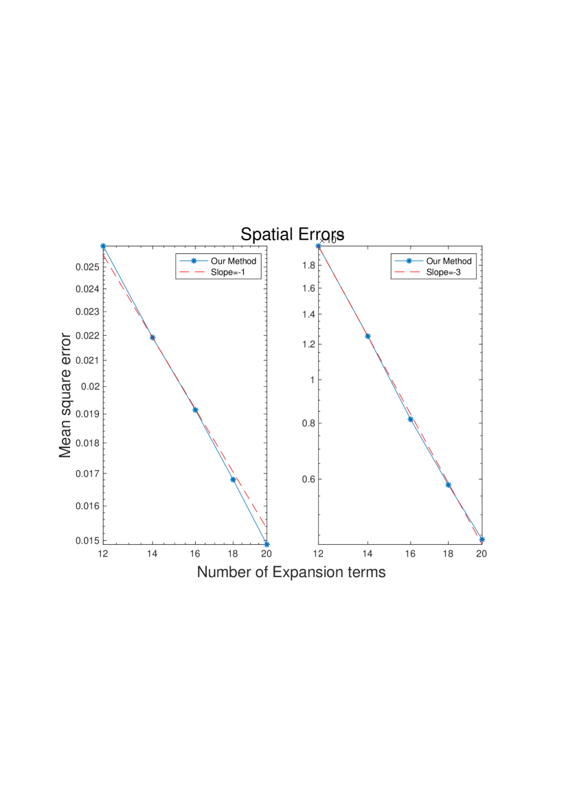
Figure 5.1. Spatial errors of 1-d stochastic Allen-Cahn equation with $g(u)=I$: (left) $q_{j}=j^{-1.001}$ and (right) $q_{j}=j^{-5.001}$.

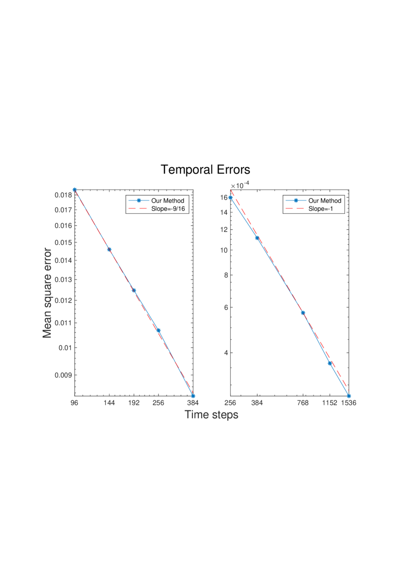
Figure 5.2. Temporal errors of 1-d stochastic Allen-Cahn equation with $g(u)=I$: (left) $q_{j}=j^{-1.001}$ and (right): $q_{j}=j^{-5.001}$.

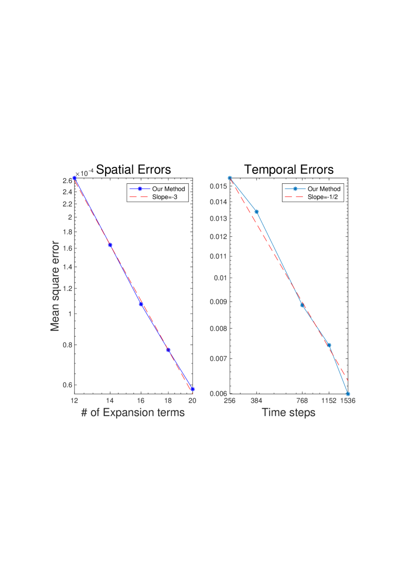
Figure 5.3. Numerical errors of 1-d Allen-Cahn equation with $g(u)=(1-u^{2})/(1+u^{2})$.

Example 5.2.

Consider the following 2-d stochastic Allen-Cahn equation:

$$\begin{cases}du=\frac{1}{2}\Delta udt+(u-u^{3})dt+g(u)dW^{Q},(x,y)\in(0,1)^{2},\\ u_{0}(x,y,0)=\sin(\pi x)\sin(\pi y),\end{cases}$$

where $g(u)=\sin(u)$ and

$$W^{Q}(t)=\sum\limits_{j_{1},j_{2}=1}^{\infty}1/\sqrt{(j_{1}^{2}+j_{2}^{2})^{3}}(\sin(j_{1}\pi x+\phi_{j_{1}}(x)))(\sin(j_{2}\pi y)+\phi_{j_{2}}(y))\beta_{j_{1},j_{2}}(t).$$

Here, $\phi(x)$ is defined in (3.18),

In the experiment, we choose $K=200$ in (5.2) to measure the error again. To balance the CPU runtime and accuracy, we truncate the first $10$ terms in each direction of $W^{Q}(t)$. In order to find the spatial convergence rate, we use the numerical solution with $N=100$ and $M=1000$ for $T=0.1$ as a surrogate of true solution. From Figure 5.4, we can clearly observe a spatial convergence rate of approximately $\mathcal{O}(N^{-3/2})$ for $N=16,17,19,21$ and $22$.

Similarly, in order to find temporal convergence rate, we use the numerical solution with $N=60$ and $M=2304$ for $T=0.5$ as a surrogate of true solution. It is clear that temporal convergence rate $\mathcal{O}(\tau^{1/2})$ for $\tau=1/64,1/72,1/96,1/128,1/144$ can be observed from Figure 5.4.

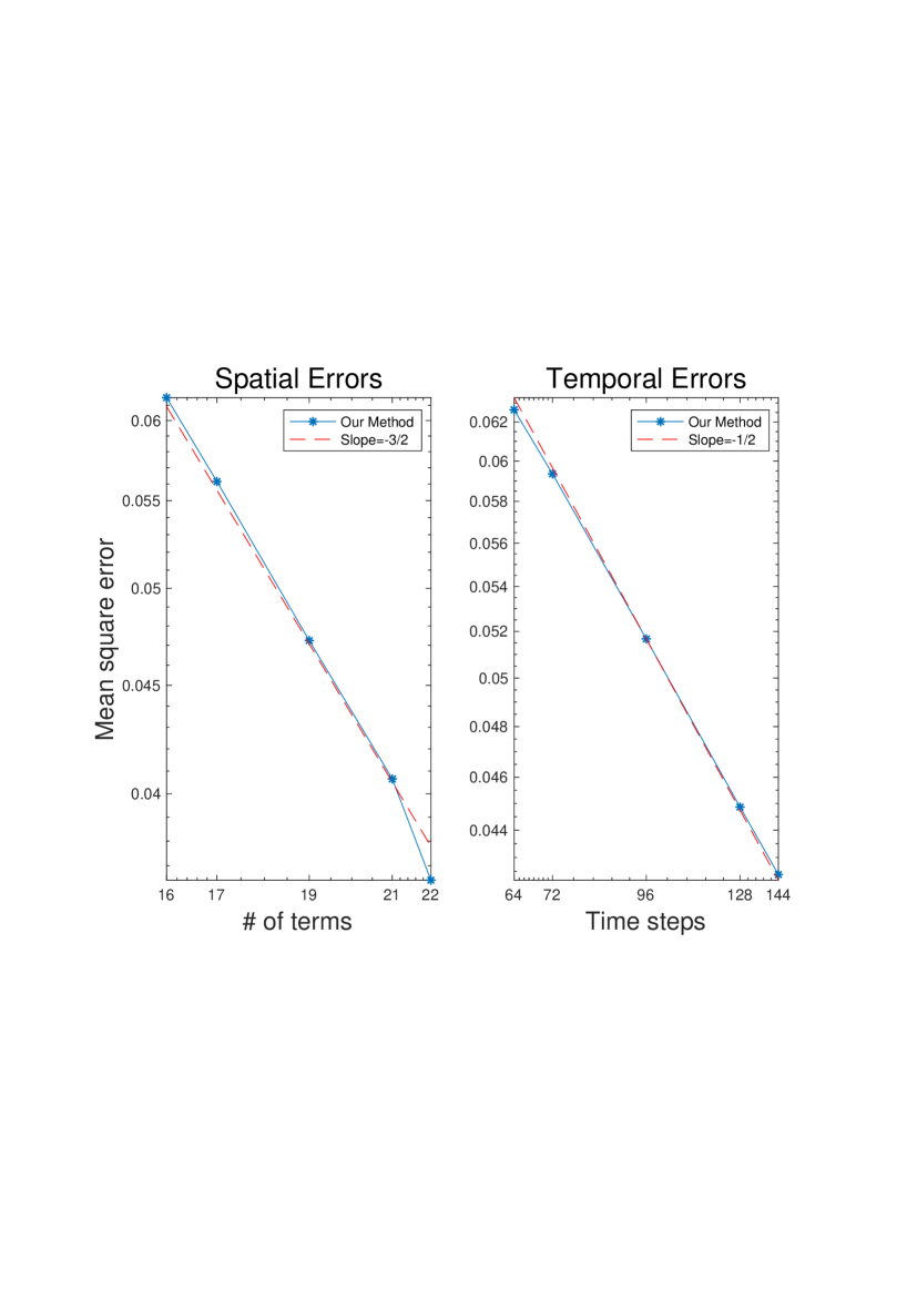
Figure 5.4. Numerical errors of 2d stochastic A-C equation.

6. Concluding remarks

We developed a fully discrete scheme for nonlinear stochastic partial differential equations with non-globally Lipschitz coefficients driven by multiplicative noise in a multi-dimensional setting. The space discretization is a Legendre spectral method, so it does not require the elliptic operator $A$ and the covariance operator $Q$ of noise in the equation commute, while can still be efficiently implemented as with a Fourier method. The time discretization is a tamed semi-implicit scheme which treats the nonlinear term explicitly while being unconditionally stable, and it avoids solving nonlinear systems at each time step. Under reasonable regularity assumptions, we established optimal strong convergence rates in both space and time for our fully discrete scheme. We also presented several numerical experiments to validate our theoretical results.

We note that the fully discrete scheme constructed in this paper can also be used for the three-dimensional case, but our error analysis is only valid for one- and two-dimensional cases.

References

- [1] Adams, R.A., Sobolev Spaces, Academic Press, New York, 1975.
- [2] E.J. Allen and S.J. Novosel and Z. Zhang, Finite element and difference approximation of some linear stochastic partial differential equations, Stoch. Stoch. reports, 64: 117-142, 1998.
- [3] D. C. Antonopoulou and G. Karali and A. Millet, Existence and regularity of solution for a stochastic Cahn-Hilliard/Allen-Cahn equation with unbounded noise diffusion, J. Differential Equations, 260: 2383-2417, 2016.
- [4] S. Becker and B. Gess and A. Jentzen and P.E. Kloeden, Strong convergence rates for explicit space-time discrete numerical approximations of stochastic Allen-Cahn equations, SAM Research Report, Eidgenössische Technische Hochschule, Zürich, 54, 2017.
- [5] S. Becker and A. Jentzen, Strong convergence rates for nonlinearity-truncated Euler-type approximations of stochastic Ginzburg–Landau equations, Stoch. Proc. Appl., 129(1): 28-69, 2019.
- [6] C. Bernardi and Y. Maday, Spectral methods, in Handbook of numerical analysis, Vol. V, 209–485, North-Holland, Amsterdam, 1997.
- [7] C. Brehier and J. Cui and J. Hong, Strong convergence rates of semidiscrete splitting approximations for the stochastic Allen–Cahn equation, IMA J. Numer. Anal., 39(4): 2096-2134, 2019.
- [8] S. Cerrai, Stochastic reaction-diffusion systems with multiplicative noise and non-Lipschitz reaction term, Probab. Theory Relat. Fields, 125: 271-304, 2003.
- [9] P. Chow, Stochastic partial differential equations, Chapman& Hall/CRC, 2007.
- [10] J. Cui and J. Hong, Strong and weak convergence rates of a apatial approximation for stochastic partial differential equation with one-sided Lipschitz coefficient, SIAM J. Numer. Anal., 57(4): 1815-1841, 2019.
- [11] G. Da Prato and J. Zabczyk, Stochastic equations in infinite dimensions, Cambridge University Press, 1991.
- [12] A. Debussche, Weak approximation of stochastic partial differential equations: the nonlinear case, Math. Comput., 80(273): 89-117, 2010.
- [13] J. Dixon and S. McKee, Weakly singular Gronwall inequalities, ZAMM Z. Angew. Math. Mech., 66: 535-544, 1986.
- [14] X. Feng and Y. Li and Y. Zhang, Finite element methods for the stochastic Allen-Cahn equation with gradient-type multiplicative noise, SIAM J. Numer. Anal., 55: 194-216, 2017.
- [15] I. Gyöngy and S. Sabanis and D. Šiška, Convergence of tamed Euler schemes for a class of stochastic evolution equations, Stoch. Partial Differ., 4(2): 225-245, 2016.
- [16] M. Hutzenthaler and A. Jentzen and P. Kloeden, Strong convergence of an explicit numerical method for SDEs with nonglobally Lipschitz continuous coefficients, Ann. Appl. Prob., 22(4): 1611-1641, 2012.
- [17] A. Jentzen and P. Kloeden and G. Winkel, Efficient simulation of nonlinear parabolic SPDEs with additive noise, Ann. Appl. Prob., 21(3): 908-950, 2011.
- [18] A. Jentzen and M. Rockner, A Milstein scheme for SPDEs, Found. Comput. Math., 15: 313-362, 2015.
- [19] A. Jentzen and P. Pušnik. Strong convergence rates for an explicit numerical approximation method for stochastic evolution equations with non-globally Lipschitz continuous nonlinearities. IMA J. Numer. Anal. 40(2): 1005–1050, 2020.
- [20] S. Larsson and A. Mesforush, Finite element approximation of the linearizedCahn-Hilliard-Cook equation, IMA J. Numer. Anal., 31:1315-1333, 2011.
- [21] W. Liu and M. Röckner, Stochastic partial differential equations: an introduction, Springer, 2015.
- [22] W. Liu and M. Röckner, SPDE in Hilbert space with locally monotone coefficients, J. Func. Anal., 259: 2902-2922, 2010.
- [23] A. Majee and A. Prohl, Optimal strong rates of convergence for a space-time discretization of the stochastic Allen-Cahn equation with multiplicative noise, Comput. Methods Appl. Math., 18:297-311, 2018.
- [24] M. Kovács and F. Lindgren and S. Larsson, Spatial approximation of stochastic convolutions, J. Comput. Appl. Math., 235: 3554-3570, 2011.
- [25] M. Kovács and S. Larsson and F. Lindgren, On the backward Euler approximation of the stochastic Allen-Cahn equation, J. Appl. Probab., 52(2): 323-338, 2015.
- [26] M. Kovács and S. Larsson and A. Mesforush, Finite element approximation of the Cahn-Hilliard-Cook equation, SIAM J. Numer. Anal., 49(6): 2407-2429, 2011.
- [27] M. Kovács and S. Larsson and A. Mesforush, Erratum: Finite element approximation of the Cahn-Hilliard-Cook equation, SIAM J. Numer. Anal., 52(5): 2594-2597, 2014.
- [28] M. Kovács and S. Larsson and F. Lindgren, On the discrettization in time of the stochastic Allen-Cahn equation, arxiv:1510.03684v3, 2018.
- [29] R. Kruse, Strong and weak approximation of semilinear stochastic evolution equations, Springer, 2014.
- [30] G. Lord and C. Powell and T. Shardlow, An introduction to computational stochastic PDEs, Cambridge university press, 2014.
- [31] A. Pazy, Semigroups of linear operators and applications to partial differential equations, Springer-Verlag, 1983.
- [32] G. Da Prato and A. Debussche, Stochastic Cahn-Hilliard equation, Nonlinear Anal. Theory Methods Appl., 26:241-263, 1996.
- [33] R. Qi and X. Wang, Optimal error estimates of Galerkin finite element methods for stochastic Allen-Cahn equation with additive noise, J. Sci. Comput., 80:1171-1194, 2019.
- [34] R. Qi and X. Wang, Error estimates of semi-discrete and fully discrete finite element methods for the Cahn-Hilliard-Cook equation, SIAM J. Numer. Anal., 58(3): 1613-1653, 2020.
- [35] J. Shen, Efficient spectral-Galerkin method I: direct solvers of second- and fourth-order equations using Legendre polynomials, SIAM J. Sci. Comput., 15(6): 1489-1505, 1994.
- [36] J. Shen, T. Tang and L.L. Wang, Spectral Methods: Algorithms, Analysis and Applications, Springer-Verlag, Berlin, Heidelberg, 2011.
- [37] V. Thomée, Galerkin Finite Element Methods for Parabolic Problems, Springer, Berlin, Heidelberg, 1997.
- [38] M. Tretyakov and Z. Zhang, A fundamental mean-square convergence theorem for SDEs with locally-Lipschitz coefficients and its applications, SIAM J. Numer. Anal., 51(6): 3135-3162, 2013.
- [39] X. Wang, Strong convergence rates of the linear implicit Euler method for the finite element discretization of SPDEs with additive noise, IMA J. Numer. Anal., 37: 965-984, 2017.
- [40] X. Wang, An efficient explicit full discrete scheme for strong approximation of stochastic Allen-Cahn equation, Stoch. Proc. Appl., 130(10): 6271-6299, 2020.
- [41] Y. Yan, Galerkin finite element methods for stochastic parabolic partial differential equations, SIAM J. Numer. Anal., 43(4): 1363-1384, 2005.