Deviance Matrix Factorization

Abstract

We investigate a general matrix factorization for deviance-based data losses, extending the ubiquitous singular value decomposition beyond squared error loss. While similar approaches have been explored before, our method leverages classical statistical methodology from generalized linear models (GLMs) and provides an efficient algorithm that is flexible enough to allow for structural zeros via entry weights. Moreover, by adapting results from GLM theory, we provide support for these decompositions by (i) showing strong consistency under the GLM setup, (ii) checking the adequacy of a chosen exponential family via a generalized Hosmer-Lemeshow test, and (iii) determining the rank of the decomposition via a maximum eigenvalue gap method. To further support our findings, we conduct simulation studies to assess robustness to decomposition assumptions and extensive case studies using benchmark datasets from image face recognition, natural language processing, network analysis, and biomedical studies. Our theoretical and empirical results indicate that the proposed decomposition is more flexible, general, and robust, and can thus provide improved performance when compared to similar methods. To facilitate applications, an R package with efficient model fitting and family and rank determination is also provided.

Keywords non-negative matrix factorization, factor models, principal component analysis

1 Introduction

Matrix factorization has a long history in statistics. In general, the problem is that given a $n$-by-$p$ data matrix $X$ where w.l.o.g. $n\geq p$, one aims to decompose $X$ into the product of two lower rank matrices that jointly summarize most of the information in $X$. With the rows of $X$ seen as samples and the columns as sample conditions or experiments, such decompositions hope to interpret the information in $X$ in factors. For instance, consider the (thin) singular value decomposition [SVD; 14] of $X$, $X=UDV^{\top}$, where $U$ is $n$-by-$p$ with orthogonal columns, that is, $U$ belongs to the Stiefel manifold $\mathcal{S}_{n,p}$, $D=\text{Diag}\{d_{1},\ldots,d_{p}\}$ is a diagonal matrix of order $p$ with $d_{1}\geq\cdots\geq d_{p}$, and $V\in O(p)$ is orthogonal. The Eckart-Young theorem [11] then states that, within rank $q$ decompositions $\mathcal{V}_{n,p}(q)=\mathbb{R}^{n\times q}\times\mathbb{R}^{p\times q}$, one solution to

$$\mathop{\text{argmin}}\limits_{(\Lambda,V)\in\mathcal{V}_{n,p}(q)}\|X-\Lambda V^{\top}\|_{F}=\\ \mathop{\text{argmin}}\limits_{(\Lambda,V)\in\mathcal{V}_{n,p}(q)}\sum_{i=1}^{n}\sum_{j=1}^{p}\big{(}X_{ij}-(\Lambda V^{\top})_{ij}\big{)}^{2}$$ (1)

is given by $\widehat{\Lambda}=U_{1:q}\text{Diag}\{d_{1},\ldots,d_{q}\}$, where $U_{1:q}$ has the first $q$ columns of $U$ and $\widehat{V}=V_{1:q}$, that is, by a rank-truncated version of $X$ according to its SVD. This result has broad applications in Statistics, the closest one being principal component analysis (PCA). In this case, regarding rows of $X$ as observations, we can center and decompose $X$ by solving

$$(\widehat{v}_{0},\widehat{\Lambda},\widehat{V})=\mathop{\text{argmin}}\limits_{v_{0}\in\mathbb{R}^{p},(\Lambda,V)\in\{\mathcal{V}_{n,p}(q):\Lambda^{\top}\text{1}_{n}=0\}}\|X-\text{1}_{n}v_{0}^{\top}-\Lambda V^{\top}\|_{F}.$$

It is known that $\widehat{v}_{0}$ contains column means and $\widehat{\Lambda}\widehat{V}^{\top}$ can be analogously obtained from the SVD of $X-\text{1}_{n}\widehat{v}_{0}^{\top}$. Here, $\widehat{\Lambda}$ corresponds to the first $q$ principal components of $X$.

The formulation in (1) is based on squared error loss, minimizing of which can be considered equivalent to maximizing a Gaussian log-likelihood. However, such a model implicitly assumes that $X\in\mathbb{R}^{n\times p}$ and often leads to spurious results in more constrained cases, for example, if $X\in\mathcal{F}^{n\times p}$ for a field $\mathcal{F}$, when $\mathcal{F}=\mathbb{N}$, $\mathcal{F}=\{0,1\}$, or even $\mathcal{F}=\mathbb{R}^{+}$. In the case that $X$ stores positive counts, that is, when $\mathcal{F}=\mathbb{N}^{+}$, one proposed improvement is non-negative matrix factorization [NMF; 30], which solves

$$\mathop{\text{argmin}}\limits_{(\Lambda,V)\in\mathcal{V}_{n,p}(q)}\sum_{i,j}X_{ij}\log\frac{X_{ij}}{(\Lambda V^{\top})_{ij}}-\big{(}X_{ij}-(\Lambda V^{\top})_{ij}\big{)}$$ (2)

and is thus based on a Kullback-Leibler (KL) loss or a Poisson log-likelihood with an identity link.

In the same way that the NMF has been successful in computer vision research, extending the factorization model with more appropriate likelihood (family) assumptions and link transformations has generated a series of benchmark methods in various applications. To name a few, in natural language processing, the Skip-gram model [36, 31] can be considered as a multinomial factorization; the Global Vectors for Word Representation [GloVe; 36] model can be considered as a log transformed PCA model with entry-wise weight specifications; in network analysis, the random dot product model [22, 52] can be considered as a Bernoulli factorization. These generalizations, along with their popularity in follow-up applications, provided empirical evidence for the importance of more realistic factorization assumptions. However, these models are tailored to specific distributions and lack generality, specially with respect to over-dispersed or heavy-tailed data, limiting their exploration and broader, more suitable use in modern applications.

1.1 Related Work: Exponential Family PCA

A more general factorization model, exponential family principal component analysis [EPCA; 9] proposes to minimize the following distance loss:

$$\mathcal{B}(X,\Lambda V^{\top})=2\sum_{i=1}^{n}\sum_{j=1}^{p}B\Big{(}X_{ij},\,\,(\Lambda V^{\top})_{ij}\Big{)},$$ (3)

where $B$ is the Bregman distance, uniquely determined by the specification of the exponential family likelihood. EPCA has generated significant interest, for example, [51, 37, 32, 33, 16, 48] focus on extending it using hierarchical structures to improve likelihood fitness and automatic rank determination. These contributions, however, have the following drawbacks:

• The hierarchical extensions tend to suffer from heavy computational costs and identifiability issues (e.g. label switching [42] and posterior collapse [49]).

• The properties of the estimator have not yet been investigated. Understanding convergence behaviour even under certain conditions will provide stronger statistical assurances for applications.

• The model provides the freedom of choosing among exponential families without providing sufficient justifications on how to choose the appropriate factorization family given the data.

• An efficient and/or robust implementation to allow entry-wise factorization priority has been wanting from practitioners. Assuming prior weights on the factorization can greatly improve model performance; as examples, see [53] for missing data and [21] for a face-centered NMF.

1.2 Our Contributions

To address the gaps in EPCA, we here revisit this factorization task under a generalized linear model [GLM; 35] framework: we assume implicitly that the data entries $X_{ij}\stackrel{{\scriptstyle\text{ind}}}{{\sim}}F(\mu_{ij},\phi_{ij})$ where $F$ belongs to the exponential family with mean ${\mathbb{E}}(X_{ij})=\mu_{ij}$ and variance $\text{Var}(X_{ij})=\phi_{ij}\mathcal{V}(\mu_{ij})$ for a variance function $\mathcal{V}(\cdot):\mathbb{R}\rightarrow\mathbb{R}$. More specifically, $F$ specifies a density/pmf $f$ of $X_{ij}$ that can be expressed parametrically as a function of canonical parameters $\theta_{ij}$ and dispersions $\phi_{ij}$ as

$$\log f(X_{ij})=\frac{X_{ij}\theta_{ij}-b(\theta_{ij})}{\phi_{ij}}+c(X_{ij},\phi_{ij}),$$

where the cumulant function $b$ is such that $b^{\prime}(\theta_{ij})=\mu_{ij}$ and $b^{\prime\prime}(\theta_{ij})=b^{\prime\prime}({b^{\prime}}^{-1}(\mu_{ij}))=\mathcal{V}(\mu_{ij})$. The terms $\phi_{ij}$ are usually specified as $\phi_{ij}=\phi/w_{ij}$ where $\phi$ is now a single dispersion parameter and $w_{ij}$ are known weights. Good references to exponential family, GLM and factor model are available correspondingly in the well-known textbook [35] and Chapter 12 of[4].

As discussed above, we relate the entry means $\mu_{ij}$ to factors $\Lambda$ and $V$ by defining the linear predictor $\eta_{ij}=(\Lambda V^{\top})_{ij}$ and by adopting a link function $g$ such that $\eta_{ij}=g(\mu_{ij})$. That is, we assume element-wisely

$$g({\mathbb{E}}(X))=\Lambda V^{\top}.$$ (4)

If $\ell(X_{ij};\eta_{ij})$ is the log-likelihood under $F$ for data entry $X_{ij}$ and parameter $\eta_{ij}$, we can then obtain the factorization $(\Lambda,V)$ by minimizing the the negative likelihood function $L(X_{ij},\eta_{ij})=\ell(X_{ij};X_{ij})-\ell(X_{ij};\eta_{ij})$, i.e. the half-deviance. With the most commonly used members of the exponential family provided in Table 1, the overall loss is then

$$\mathcal{L}(X,\Lambda V^{\top})=\sum_{i=1}^{n}\sum_{j=1}^{p}w_{ij}L\Big{(}X_{ij},\,\,g^{-1}\big{(}(\Lambda V^{\top})_{ij}\big{)}\Big{)},$$ (5)

where we made the dependency on dispersion weights explicit. To emphasize these connections to GLM methodology, we denote our method as deviance matrix factorization (DMF).

While the implicit assumption of a data generative process might seem to be too restrictive, here it only serves to define the data loss $L$ in (5). In practice, as we show here, the factorization only really requires the specification of $L$ up to the second moments of the log-likelihood, as usual in GLMs under quasi-likelihood assumptions [50]. In this way, our proposed approach inherits robustness to model misspecification.

While we regard the methods we discuss here as descriptive, similarly to PCA, there are close connections to factor analysis, which, in turn, aims at inferring covariance structure. We benefited from recent advances in this field, under a Gaussian error assumption, to investigate factorization consistency [25, 2] and determine the factorization rank $q$ [38, 46, 12]. Here we extend these results and propose a maximum eigengap rule to specify $q$. Compared to related EPCA methods, our methods are simpler and more efficient while achieving similar statistical performance. To summarize, as we show later, our DMF enjoys the following advantages:

• To appropriately model a wider variety of real world data, we extended PCA and NMF to a factorization under a general exponential family assumption.

• To avoid identifiability issues, we constraint the factors $\Lambda$ and $V$ to be orthogonal frames and thus unique, yielding a more robust and efficient algorithm.

• Under some extra conditions, we extend GLM consistency [8] to DMF factors.

• We adapt a generalized Hosmer-Lemeshow test [45] to determine the adequacy of a factorization family/link choice.

• By specifying a link function $g$ and entry weights $w_{ij}$, we can better accommodate factorizations for various applications such as matrix completion and residual boosting[18, 26].

1.3 Organization of the Paper

We start in Section 2 by formally introducing the deviance matrix factorization and discussing how we tackle identifiability issues and centering. Next, in Section 3, we devise a flexible and robust algorithm to produce DMFs. In Section 4 we offer theoretical guarantees on issues that would lead to spurious results if left unanswered: we first show that the DMF exists and is consistent, and then discuss how to determine the factorization rank and test the adequacy of family and link choices. In Section 5 we supplement these developments with extensive simulations and case studies using benchmark datasets from many fields. As we show, the proposed methods yield good results and better performance than traditional methods in practice, with real-world datasets favoring over-dispersed distributions such as the negative binomial. Finally, Section 6 concludes with a discussion and offers directions for future work.

2 Deviance Matrix Factorization

In this section, we formally introduce our factorization model along with some details on how we address the identifiability and incorporate prior decomposition structure.

In a connection to PCA can be considered as a model assuming ${\mathbb{E}}(X)=\Lambda V^{\top}$ with $X$ following multivariate Gaussian distribution, our deviance matrix factorization assumes $g({\mathbb{E}}(X))=\Lambda V^{\top}$ with $X$ following natural exponential family distribution. Borrowing the notations from generalized linear models [35], our goal then is to decompose $X$ as an entry-wise function of $\Lambda V^{\top}$, with approximation error measured by the loss in (5). That is, we seek the DMF

$$(\widehat{\Lambda},\widehat{V})=\mathop{\text{argmin}}\limits_{(\Lambda,V)\in\mathcal{V}_{n,p}(q)}\mathcal{L}(X,\Lambda V^{\top}).$$ (6)

For example, using a Gaussian loss, $L(x,y)=(x-y)^{2}/2$, and an identity link we recover (1), while a Poisson loss, equivalent here to KL loss, again with an identity link yields a non-negative matrix decomposition (2). Table 1 lists more examples with correspondences between a distribution in the exponential family and their respective half-deviance loss functions and canonical links. The link function $g(\mu)$ is given in the canonical form, but in general can be any smooth and invertible function w.r.t field $\mathcal{F}$.

Distribution $F$	Domain	Link $g(\mu)$	Variance function $\mathcal{V}(\mu)$	Loss $L(x,\mu)$
Gaussian	$\mathbb{R}$	$\mu$	$1$	$(x-\mu)^{2}/2$
Poisson	$\mathbb{N}_{+}$	$\log\mu$	$\mu$	$x\log(x/\mu)-(x-\mu)$
Gamma	$\mathbb{R}_{+}$	$\mu^{-1}$	$\mu^{2}$	$(x-\mu)/\mu-\log(x/\mu)$
Bernoulli	$[0,1]$	$\log[\mu/(1-\mu)]$	$\mu(1-\mu)$	$x\log(x/\mu)+$
				$(1-x)\log[(1-x)/(1-\mu)]$
Negative binomial $(\phi)$	$\mathbb{N}_{+}$	$\log[\mu/(\mu+\phi)]$	$\mu+\mu^{2}/\phi$	$x\log(x/\mu)-$
				$\phi\log[(x+\phi)/(\mu+\phi)]$

Table 1: Distributions and their respective canonical links and half-deviance loss functions.

2.1 Identifiability

Denote by $GL(q,\mathbb{R})$ the generalized linear space with rank $q$ and domain $\mathbb{R}$. If $\widehat{\Lambda}$ and $\widehat{V}$ are a solution to (6) then an arbitrary $M\in GL(q,\mathbb{R})$ yields a new solution with $\widetilde{\Lambda}=\widehat{\Lambda}M^{-\top}$ and $\widetilde{V}=\widehat{V}M$ since then $\widehat{\Lambda}\widehat{V}^{\top}=\widetilde{\Lambda}\widetilde{V}^{\top}$. To guarantee identifiability so that, as in the SVD, our decomposition is unique, we then require any solution $(\Lambda,V)$ is such that

1. $V$ has orthogonal columns, i.e. $V^{\top}V=I_{q}$ and so $V$ belongs to the Stiefel manifold $\mathcal{S}_{p,q}$;

2. $\Lambda$ has scaled pairwise orthogonal columns, that is, $\Lambda=UD$ with $U\in\mathcal{S}_{n,q}$ and $D=\text{Diag}\{d_{1},\ldots,d_{q}\}$ with $d_{1}\geq\cdots\geq d_{q}$ so that $\Lambda^{\top}\Lambda=D^{2}$. We denote this space for $\Lambda$ as $\widetilde{\mathcal{S}}_{n,q}$.

In this case, $\widetilde{V}\in\mathcal{S}_{p,q}$ implies that $\widetilde{V}^{\top}\widetilde{V}=M^{\top}M=I_{q}$, that is, $M\in O(q)$ is orthogonal, and so $M^{-\top}=M$. Moreover, if $\widehat{\Lambda}^{\top}\widehat{\Lambda}=\widehat{D}^{2}$ then $\widetilde{\Lambda}^{\top}\widetilde{\Lambda}=M^{\top}\widehat{D}^{2}M\doteq\widetilde{D}^{2}$, that is, $\widehat{D}^{2}M=M\widetilde{D}^{2}$. But the only way that $M$ commutes with diagonal matrices is if $M=I_{q}$ and $\widehat{D}=\widetilde{D}$ (up to sign changes, as in the SVD). Thus, we have just shown that

$$\min_{(\Lambda,V)\in\mathcal{V}_{n,p}(q)}\mathcal{L}(X,\Lambda V^{\top})=\min_{\Lambda\in\widetilde{\mathcal{S}}_{n,q},V\in\mathcal{S}_{p,q}}\mathcal{L}(X,\Lambda V^{\top}),$$

with the solution to the right-hand side being unique. In practice, we can always identify a unique solution $(\widehat{\Lambda},\widehat{V})\in\widetilde{\mathcal{S}}_{n,q}\times\mathcal{S}_{p,q}$ from a general solution $(\widetilde{\Lambda},\widetilde{V})\in\mathcal{V}_{n,p}(q)$ by obtaining the $q$-rank SVD decomposition $\widetilde{\Lambda}\widetilde{V}^{\top}=UD\widehat{V}^{\top}$ and setting $\widehat{\Lambda}=UD$.

2.2 Centering

We can capture a known prior structure $\Lambda_{0}\in\mathbb{R}^{n\times q_{0}}$ of rank $q_{0}$ in the decomposition by solving

$$\min_{V_{0}\in\mathbb{R}^{p\times q_{0}},(\Lambda,V)\in\{\mathcal{V}_{n,p}(q)\,:\,\Lambda^{\top}\Lambda_{0}=0\}}\mathcal{L}(X,\Lambda_{0}V_{0}^{\top}+\Lambda V^{\top}),$$ (7)

where the $q_{0}$ orthogonality constraints $\Lambda^{\top}\Lambda_{0}=0$ avoid redundancies. As an example, the most common use of this setup is when $\Lambda_{0}=\mathbf{1}_{n}$ and $V_{0}$ serves as the center of $X$, similar to PCA [20] under Gaussian loss.

We can obtain a solution $(\widehat{V}_{0},\widehat{\Lambda},\widehat{V})$ to (7) directly from a solution $(\Lambda,V)$ to (6): if $H_{0}=\Lambda_{0}(\Lambda_{0}^{\top}\Lambda_{0})^{-1}\Lambda_{0}^{\top}$ is the projection matrix into the space spanned by the columns of $\Lambda_{0}$, then

$$\Lambda V^{\top}=H_{0}\Lambda V^{\top}+(I_{n}-H_{0})\Lambda V^{\top}=\Lambda_{0}\underbrace{(\Lambda_{0}^{\top}\Lambda_{0})^{-1}\Lambda_{0}^{\top}\Lambda V^{\top}}_{\doteq\widehat{V}_{0}}+\underbrace{(I_{n}-H_{0})\Lambda V^{\top}}_{\doteq\widehat{\Lambda}\widehat{V}^{\top}},$$

where, as in the previous section, $\widehat{\Lambda}\in\widetilde{\mathcal{S}}_{n,q}$ and $\widehat{V}\in\mathcal{S}_{p,q}$ are computed from the $q$-rank SVD decomposition of $(I_{n}-H_{0})\Lambda V^{\top}$. Note that since $\Lambda_{0}^{\top}\widehat{\Lambda}\widehat{V}^{\top}=\Lambda_{0}^{\top}(I_{n}-H_{0})\Lambda V^{\top}=0$ and $\widehat{V}$ is full rank, we have $\Lambda_{0}^{\top}\widehat{\Lambda}=0$ as required.

3 Decomposition

From the last section we know that we just need to solve the unconstrained version in (6) and post-process the solution to identify it even after centering. Moreover, this post-process ensures an unique deviance factorization. In this section we describe a method to deviance decompose the input matrix $X$. Incorporating the entry-wise factorization weights $w_{ij}$, we modify the GLM re-weighted least squares [IRLS; 35] algorithm with a normalization step to achieve higher numerical stability and to avoid overflows. The optimization problem in (6) is clearly not jointly convex on both factors $\Lambda$ and $V$, but, as in the SVD, it is convex on each factor individually, so we alternate Fisher scoring updates for one factor conditional on the other factor.

3.1 Deviance Factorization

Let us first define the linear predictor $\eta_{ij}=\sum_{k=1}^{q}\Lambda_{ik}V_{jk}$. From the distribution $F$ we have the log-likelihood in terms of the canonical parameter $\theta_{ij}$ and up to a constant as

$$-L(X_{ij},\theta_{ij})=\frac{w_{ij}}{\phi}\big{(}X_{ij}\theta_{ij}-b(\theta_{ij})\big{)},$$

where $w_{ij}$ are weights and $b$ and $\phi$ are the cumulant function and dispersion parameter of $F$, respectively. The cumulant allows us to define $\mu_{ij}=b^{\prime}(\theta_{ij})$ as the mean of $X_{ij}$ and $\mathcal{V}(\mu_{ij})=b^{\prime\prime}(\theta_{ij})$ as the variance function. Finally, the means and linear predictors are related by the link function $g$, $\eta_{ij}=g(\mu_{ij})$.

With $\beta$ being an arbitrary entry of either $\Lambda$ or $V$, we then have

$$\begin{split}\frac{\partial L(X_{ij},\mu_{ij})}{\partial\beta}&=\frac{\partial\eta_{ij}}{\partial\beta}\frac{\partial\mu_{ij}}{\partial\eta_{ij}}\Bigg{(}\frac{\partial\mu_{ij}}{\partial\theta_{ij}}\Bigg{)}^{-1}\frac{\partial L(X_{ij},\theta_{ij})}{\partial\theta_{ij}}\\ &=-\frac{\partial\eta_{ij}}{\partial\beta}\frac{{g^{-1}}^{\prime}(\eta_{ij})}{V(\mu_{ij})}\frac{w_{ij}}{\phi}(X_{ij}-\mu_{ij})\doteq-\frac{\partial\eta_{ij}}{\partial\beta}G_{ij}.\end{split}$$

For $k=1,\ldots,q$, we then have the scores

$$\frac{\partial\mathcal{L}}{\partial\Lambda_{ik}}=-2\sum_{j=1}^{p}G_{ij}V_{jk}\quad\text{and}\quad\frac{\partial\mathcal{L}}{\partial V_{jk}}=-2\sum_{i=1}^{n}G_{ij}\Lambda_{ik},$$

that is, $\partial\mathcal{L}/\partial\Lambda=-2GV$ and $\partial\mathcal{L}/\partial V=-2G^{\top}\Lambda$. Similarly, taking both $\beta$ and $\gamma$ to be arbitrary entries in either $\Lambda$ or $V$, we obtain

$${\mathbb{E}}\Bigg{[}\frac{\partial^{2}L(X_{ij},\mu_{ij})}{\partial\beta\partial\gamma}\Bigg{]}=\frac{\partial\eta_{ij}}{\partial\beta}\frac{\partial\eta_{ij}}{\partial\gamma}\frac{w_{ij}}{\phi}\frac{{{g^{-1}}^{\prime}(\eta_{ij})}^{2}}{V(\mu_{ij})}\doteq\frac{\partial\eta_{ij}}{\partial\beta}\frac{\partial\eta_{ij}}{\partial\gamma}S_{ij}.$$

Thus, for example, with $\beta=\Lambda_{ik}$ and $\gamma=\Lambda_{lm}$ we have

$${\mathbb{E}}\Bigg{[}\frac{\partial^{2}\mathcal{L}}{\partial\Lambda_{ik}\partial\Lambda_{lm}}\Bigg{]}=2\sum_{j=1}^{p}V_{jk}V_{jm}S_{ij}\delta_{il},$$

where $\delta$ is the Kronecker delta.

3.1.1 $\Lambda$-step

Now, denoting $\boldsymbol{\lambda}=\text{vec}(\Lambda)$, the Fisher scoring update for $\Lambda$ at the $t$-th iteration is

$$\boldsymbol{\lambda}^{(t+1)}=\boldsymbol{\lambda}^{(t)}-{\mathbb{E}}\Bigg{[}\frac{\partial^{2}\mathcal{L}}{\partial\boldsymbol{\lambda}\partial\boldsymbol{\lambda}^{\top}}(\boldsymbol{\lambda}^{(t)})\Bigg{]}^{-1}\frac{\partial{\mathcal{L}}}{\partial\boldsymbol{\lambda}}(\boldsymbol{\lambda}^{(t)})\doteq\boldsymbol{\lambda}^{(t)}+H_{\lambda}(\boldsymbol{\lambda}^{(t)})^{-1}\text{vec}(G^{(t)}V^{(t)}).$$ (8)

The Hessian matrix $H_{\lambda}$ is such that

$$(H_{\lambda})_{ik,lm}=\sum_{j}V_{jk}V_{jm}S_{ij}\delta_{il}.$$

Thus, since $(H_{\lambda}\boldsymbol{\lambda})_{ik}=\sum_{j}\sum_{m}V_{jk}V_{jm}S_{ij}\Lambda_{im}$, we have that

$$H_{\lambda}\boldsymbol{\lambda}=\text{vec}\Big{(}\big{(}S\circ(\Lambda V^{\top})\big{)}V\Big{)},$$

where $\circ$ is the Hadamard elementwise product. After pre-multiplication by $H_{\lambda}(\boldsymbol{\lambda}^{(t)})$ in (8) the update then becomes, in matrix form,

$$\big{(}S^{(t)}\circ(\Lambda^{(t+1)}{V^{(t)}}^{\top})\big{)}V^{(t)}=\big{(}S^{(t)}\circ(\Lambda^{(t)}{V^{(t)}}^{\top})\big{)}V^{(t)}+G^{(t)}V^{(t)}.$$ (9)

To simplify the notation, let us drop all $t$ iteration superscripts with the exception of $\Lambda$ terms and define $D_{i\cdot}\doteq\text{Diag}\{S_{i\cdot}^{(t)}\}$, where $S_{i\cdot}$ denotes the $i$-th row of $S$. Let us also denote by $\lambda_{i}$ the $i$-th row of $\Lambda$; we then want $\Lambda^{(t+1)}=[\lambda_{1}^{(t+1)}\cdots\lambda_{n}^{(t+1)}]^{\top}$. We write (9) as

$$\big{(}(\Lambda^{(t+1)}V^{\top})\circ S\big{)}V=\begin{bmatrix}{\lambda_{1}^{(t+1)}}^{\top}V^{\top}D_{1\cdot}V\\ \vdots\\ {\lambda_{n}^{(t+1)}}^{\top}V^{\top}D_{n\cdot}V\end{bmatrix}=\big{(}(\Lambda^{(t)}V^{\top})\circ S\big{)}V+GV.$$

Taking the $i$-th row, $i=1,\ldots,n$, and transposing we see that we just need to solve

$$V^{\top}D_{i\cdot}V\lambda_{i}^{(t+1)}=V^{\top}D_{i\cdot}(V\lambda_{i}^{(t)}+D_{i\cdot}^{-1}G_{i\cdot})\doteq V^{\top}D_{i\cdot}Z_{i\cdot}^{(t)},$$ (10)

where $Z^{(t)}$ is the working response,

$$Z_{ij}^{(t)}=\eta_{ij}^{(t)}+\frac{G_{ij}^{(t)}}{S_{ij}^{(t)}}=\eta_{ij}^{(t)}+\frac{X_{ij}-\mu_{ij}^{(t)}}{{g^{-1}}^{\prime}(\eta_{ij}^{(t)})}.$$ (11)

That is, to obtain each $\lambda_{i}^{(t+1)}$ we just regress $Z_{i\cdot}^{(t)}$ on $V^{(t)}$ with weights $S_{i\cdot}^{(t)}$. Note that since $Z^{(t)}$ is independent of $\phi$, we can take the variance weights $S_{ij}$ to be independent of $\phi$ when finding $\lambda_{i}^{(t+1)}$:

$$S_{ij}^{(t)}=w_{ij}\frac{{g^{-1}}^{\prime}(\eta_{ij}^{(t)})^{2}}{V(\mu_{ij}^{(t)})}.$$ (12)

3.1.2 $V$-step

Similarly, the Fisher scoring update for $V$ at the $t$-th iteration is

$$\big{(}S^{(t)}\circ(\Lambda^{(t)}{V^{(t+1)}}^{\top})\big{)}^{\top}\Lambda^{(t)}=\big{(}S^{(t)}\circ(\Lambda^{(t)}{V^{(t)}}^{\top})\big{)}^{\top}\Lambda^{(t)}+{G^{(t)}}^{\top}\Lambda^{(t)}.$$ (13)

Denoting $v_{j}$ as the $j$-th row of $V$ our goal now is to obtain $V^{(t+1)}=[v_{1}^{(t+1)}\cdots v_{p}^{(t+1)}]^{\top}$. We again drop the iteration superscripts and denote $D_{\cdot j}\doteq\text{Diag}\{S_{\cdot j}^{(t)}\}$, where $S_{\cdot j}$ denotes the $j$-th column of $S$. The update in (13) is then, after transposition,

$$\Lambda^{\top}\big{(}S\circ(\Lambda{V^{(t+1)}}^{\top})\big{)}=[\Lambda^{\top}D_{\cdot 1}\Lambda v_{1}\cdots\Lambda^{\top}D_{\cdot p}\Lambda v_{p}]=\Lambda^{\top}\big{(}S\circ(\Lambda{V^{(t)}}^{\top})\big{)}+\Lambda^{\top}G.$$

But then we can just solve columnwise, for $j=1,\ldots,p$,

$$\Lambda^{\top}D_{\cdot j}\Lambda v_{j}^{(t+1)}=\Lambda^{\top}D_{\cdot j}(\Lambda v_{j}^{(t)}+D_{\cdot j}^{-1}G_{\cdot j})\doteq\Lambda^{\top}D_{\cdot j}Z_{\cdot j}^{(t)},$$ (14)

that is, to obtain $v_{j}^{(t+1)}$ we just regress $Z_{\cdot j}^{(t)}$ on $\Lambda^{(t)}$ with weights $S_{\cdot j}^{(t)}$.

3.1.3 Algorithm DMF

Having both scoring updates we just need to alternate between $\Lambda$ and $V$-steps until convergence of the deviance loss in (5). Convergence can be assessed by relative change in $\mathcal{L}$ between iterations. To kickstart the procedure, we can first follow another common procedure in GLM fitting and initialize $\mu_{ij}^{(0)}$ entrywise as an $F$-perturbed version of $X_{ij}$—e.g, $\mu_{ij}^{(0)}=X_{ij}+\epsilon$ with a small $\epsilon>0$ if $F$ is Poisson. Then, with $\eta_{ij}^{(0)}=g(\mu_{ij}^{(0)})$, we set $V^{(0)}$ as the first $q$ columns of the transpose of $[\eta_{ij}^{(0)}]_{i,j}$. Note that we do not need to initialize $\Lambda^{(0)}$ since $\Lambda^{(1)}$ only needs $V^{(0)}$. Finally, because for an arbitrary diagonal matrix $D$ of order $q$ we have

$$\Lambda V^{\top}=\Lambda D^{-1}DV^{\top}=(\Lambda D^{-1})(VD)^{\top},$$

to achieve higher numerical stability and avoid overflows we fix the scale of the columns of $\Lambda$ and $V$ by normalizing the columns of $V^{(t)}$ before a $\Lambda$-step and the columns of $\Lambda^{(t+1)}$ before a $V$-step.

We summarize this specialized version of iteratively reweighted least squares (IRLS) in Algorithm 1. Given a continuous and differentiable link $g$, we can thus see that the algorithm converges to at least a stationary point by Proposition 2.7.1 in [3]. The general solution to the stationary point optimization problem is either running the algorithm multiple times with random initialization or initializing the parameters $\widehat{\Lambda},\widehat{V}$ with the data $X$ information. The GLM framework has initialization algorithm leverages the data $X$ information, we here adopted the GLM initialization as the remedy to the stationary point optimization problem. A concrete implementation as R package dmf is available in the supplement.

$\triangleright$ Input : $n$-by-$p$ data matrix $X$.

$\triangleright$ Parameters : Distribution $F$ and link function $g$; decomposition rank $q$.

$\triangleright$ Output : $(\widehat{\Lambda},\widehat{V})\in\mathcal{V}_{n,p}(q)$ solution to (6).

$\triangleright$ Initialization:

for $i=1,\ldots,n$ and $j=1,\ldots,p$ do

       Set $\mu_{ij}^{(0)}$ as an $F$-perturbed version of $X_{ij}$ and $\eta_{ij}^{(0)}=g(\mu_{ij}^{(0)})$;

      

Set $V^{(0)}$ as the first $q$ columns of $[\eta_{ij}^{(0)}]_{i=1,\ldots,n;j=1,\ldots,p}^{\top}$;

$\triangleright$ Cyclic scoring iteration:

for $t=0,1,\ldots$ (until convergence) do

       Given $\eta^{(t)}$ and $\mu^{(t)}$, compute working responses $Z^{(t)}$ as in (11) and variance weights $S^{(t)}$ as in (12);

       $\triangleright$ $\Lambda$-step:

       Normalize the columns of $V^{(t)}$;

       for $i=1,\ldots,n$ do $\triangleright$ find $\Lambda^{(t+1)}$ in (9)

             Regress $Z_{i\cdot}^{(t)}\sim V^{(t)}$ with weights $S_{i\cdot}^{(t)}$ to obtain $\lambda_{i}^{(t+1)}$ in (10);

            

      $\triangleright$ $V$-step:

       Normalize the columns of $\Lambda^{(t+1)}$;

       for $j=1,\ldots,p$ do $\triangleright$ find $V^{(t+1)}$ in (13)

             Regress $Z_{\cdot j}^{(t)}\sim\Lambda^{(t+1)}$ with weights $S_{\cdot j}^{(t)}$ to obtain $v_{j}^{(t+1)}$ in (14);

            

      for $i=1,\ldots,n$ and $j=1,\ldots,p$ do $\triangleright$ update $\eta$ and $\mu$

             Set $\eta_{ij}^{(t+1)}=\sum_{k=1}^{q}\Lambda_{ik}^{(t+1)}V_{jk}^{(t+1)}$ and $\mu_{ij}^{(t+1)}=g^{-1}(\eta_{ij}^{(t+1)})$;

            

      

Algorithm 1 Deviance matrix factorization (DMF)

4 Theoretical and Practical Guarantees

While Algorithm 1 enables us to find deviance matrix factorizations, there are still two issues to tackle: finding adequate exponential family distributions in the formulation of the DMF and a suitable, parsimonious decomposition rank. In this section,we provide solutions for these two problems, along with theoretical guarantees for the good performance of the DMF. We start by extending the consistency of GLM estimators to the DMF, and then discuss methods to determine factorization family and rank next.

4.1 Strong Consistency of DMF Estimator

In this section, we justify our DMF estimator $\widehat{\eta}=\widehat{\Lambda}\widehat{V}^{\top}$ fitted using Algorithm 1 as a consistent estimator of $\Lambda V^{\top}$ under mild conditions. Our setup is motivated by the setup in [38] and [7] which assume fixed rank $q$ but diverging $p/n\rightarrow c$ for some constant $c>0$. The difference is that these references assume i.i.d. Gaussian errors $X_{ij}=\Lambda_{i}^{\top}V_{j}+A_{i}\epsilon B_{j}$ for deterministic matrices $A\in\mathbb{R}^{n\times n}$ and $B\in\mathbb{R}^{p\times p}$. Here we assume that the error is non-Gaussian and not necessarily additive on the $\eta\equiv\Lambda V^{\top}$. To simplify the notation from now on we denote $m(\cdot)=g^{-1}(\cdot)$, so $\mu_{ij}={\mathbb{E}}(X_{ij})=m\big{(}(\Lambda V^{\top})_{ij}\big{)}$.

Theorem 4.1.

Let $\lambda_{l,n,p}(\mathcal{M})$ to be the $l$-th largest eigenvalue of matrix $\mathcal{M}\in\mathbb{R}^{n\times p}$. $\lambda_{l,n,p}(\mathcal{M})$ can take limits of $n,p$ since the matrix input $\mathcal{M}$ is of dimension $n\times p$. We abbreviated the notation as $\lambda_{i}(\mathcal{M})\equiv\lambda_{i,n,p}(\mathcal{M})$. Under the following conditions:

1. $\lim\limits_{n,p\rightarrow\infty}\lambda_{q}((\Lambda^{\top}\Lambda)V^{\top}V)=\infty$

2. $e_{ij}=X_{ij}-\mu_{ij}$ is defined as the fitted residual. For any random variables $c_{ij}$ satisfying $\sum_{j=1}^{p}c^{2}_{ij}<\infty$ for fix $i$ and $\sum_{i=1}^{n}c^{2}_{ij}<\infty$ for fix $j$, the fitted residual $c_{ij}e_{ij}$ are such that:

   • $\sum_{j=1}^{p}c_{ij}e_{ij}$ converges a.s as $p\rightarrow\infty$ $\forall i=1,\cdots,n$

   • $\sum_{i=1}^{n}c_{ij}e_{ij}$ converges a.s as $n\rightarrow\infty$ $\forall j=1,\cdots,p$

3. With $m^{\prime}(t)=\frac{dm(t)}{dt}>0$, $m$ is continuously differentiable.

4. $\sup_{i\leq n}\|\Lambda_{i}\|_{2}<\infty$ and $\sup_{j\leq p}\|V_{j}\|_{2}<\infty$ for every $n$ and $p$

The DMF estimator is strongly consistent in the sense that :

$$\widehat{\Lambda}\xrightarrow{a.s.}\Lambda,\widehat{V}\xrightarrow{a.s.}V\text{ as }n,p\rightarrow\infty.$$

where $\Lambda$ and $V$ are defined as infinite dimensional matrices.

Remark 4.1.

Notice that condition C1 restricts the significance of the principal components and when we impose the identifiability of DMF, we have the condition to be simplified into $\lim\limits_{n,p\rightarrow\infty}\lambda_{q}((\Lambda^{\top}\Lambda)V^{\top}V)=\lim\limits_{n,p\rightarrow\infty}\lambda_{q}({\Lambda}^{\top}\Lambda)=\infty$. Similar conditions have been frequently used in [7, 38, 12].
Condition C2 puts restrictions on the magnitude of factorization noise. For instance, a similar condition, but with $c_{i}$ being deterministic, has been assumed in [8]. It essentially implies that we need a careful balance on the significance of the principal components such that condition C1 is satisfied and the variance does not grow unbounded.
Conditions C3 and C4 are additional assumptions required to compensate the non-linearity imposed by GLM type link function $g(\cdot)$. A similar condition is also assumed in [8]. Compared to condition C1, condition C4 is asking for non-dominating principal component $\Lambda$ and projection matrix $V$.

4.2 Factorization family determination

Due to the setup of matrix factorization, the number of parameters in the DMF will increase according to the sample size. This has prevented us from directly applying the asymptotic distribution of $\chi^{2}$ or deviance statistics to assess goodness of fit, as in regular GLMs. With degrees of freedom specified from stratified residual groups, [43] first generalized the Hosmer-Lemeshow test to other GLM families by deriving its asymptotic distribution, but such a generalized testing statistic requires determining a kernel bandwidth for variance estimation. To overcome bandwidth selection and the curse of dimensionality, [45] provided a more straightforward generalized Hosmer-Lemeshow test statistic with an empirical power simulation study to justify its performance. Although these test statistics are proposed within an usual GLM regression framework, we have been able to justify their use of a naive generalized Hosmer-Lemeshow test within the context of our matrix decomposition. The generalized Hosmer-Lemeshow test is based upon the idea of grouping the model fitted values $\widehat{\eta}_{ij}$ according to their magnitude and standardizing their summation into a chi-square statistic [44]. Consequently, to ensure we have enough normalized samples to judge for normality, the general guideline is choosing the number of groups $G$ such that $G\geq 15$ and to have each group containing at least ten observations—taking a dataset with 150 observations as an example, we could choose the $k$-th group threshold $u_{k}$ according to the 15th quantile of $\widehat{\eta}$.

We adopt a notation similar to [44], defined below:

$$R_{n,p}^{1}(u_{k}) =\frac{1}{\sqrt{np}}\sum_{i=1}^{n}\sum_{j=1}^{p}1_{\{\widehat{\eta}_{ij}\leq u_{k}\}}[X_{ij}-m(\widehat{\eta}_{ij})],\text{~{}for~{}}k=1,\ldots,G$$ (15)

$$T_{n,p}^{1} =\{R_{n,p}^{1}(u_{k})-R_{n,p}^{1}(u_{k-1})\}_{k=2}^{G}$$

$$D^{1}_{n,p} =\text{Diag}\Big{(}\frac{1}{np}\sum_{i=1}^{n}\sum_{j=1}^{p}\mathcal{V}(m(\widehat{\eta}_{ij}))1_{\{u_{k-1}<\widehat{\eta}_{ij}\leq u_{k}\}}\Big{)}$$

$$s^{2}_{n,p}(k) =\sum_{i=1}^{n}\sum_{j=1}^{p}1_{\{u_{k-1}<\eta_{ij}\leq u_{k}\}}(X_{ij}-m(\eta_{ij}))^{2},\text{~{}for~{}}k=2,\ldots,G$$

Specifically, $R_{n,p}^{1}(u_{k})$ is the empirical residual process given estimator $\widehat{\eta}$ and cutoff point $u_{k}$; based upon $R_{n,p}^{1}(u_{k})$, we define a $G$-long vector $T_{n,p}^{1}$ with $k$-th element being the empirical residual w.r.t. cutoffs $(u_{k-1},u_{k})$; $D^{1}_{n,p}$ is a diagonal matrix with entries being the empirical variances of $T^{1}_{n,p}$; $s^{2}_{n,p}(k)$ is the (summed) variance for group $k$ under true parameter $\eta$. Moreover, we denote by $R_{n,p},T_{n,p},D_{n,p}$ the respective processes under true parameters $\eta_{ij}$, instead of $\widehat{\eta}_{ij}$. $\mathcal{V}(\cdot)$ here is the variance function as defined in Table 1. Based on this notation, we propose Theorem 4.2 to assess a factorization family:

Theorem 4.2.

Assume that $F$ is the correct factorization family. Under conditions (F1)–(F3),

1. $\widehat{\eta}\rightarrow\eta\ a.s.$ element-wise, which can be justified by Theorem 4.1;

2. For $\delta s_{n,p}(k)>0$, we have $\{T_{k}\}_{k=2}^{G}=\{1_{\{u_{k-1}<\eta_{ij}\leq u_{k}\}}(X_{ij}-m(\eta_{ij}))\}_{k=2}^{G}$ satisfies

   $$\frac{1}{s^{2}_{n,p}(k)}\sum_{i=1}^{n}\sum_{j=1}^{p}{\mathbb{E}}[T_{k}^{2}1_{\{|T_{k}|>\delta s_{n,p}(k)\}}]\xrightarrow{a.s.}0$$

   for $k=2,\ldots,G$;

3. $\sigma^{2}_{T_{k}}=\phi_{ij}\int_{u_{k-1}}^{u_{k}}\mathcal{V}(X_{ij}|\eta_{ij}=t)F(dt)=c_{k}<\infty$ for $k=2,\ldots,G$;

and for $u_{1}<u_{2}<\cdots<u_{G}$ a partition on the support of $\eta$, we have

$$\widehat{T}(n,p) =(T_{n,p}^{1})^{\top}(D^{1}_{n,p})^{-1}T_{n,p}^{1}\xrightarrow[n,p\rightarrow\infty]{d}\chi^{2}_{G-1}$$ (16)

Remark 4.2.

Condition F1 is satisfied by following conditions C1–C4 in our Theorem 4.1, condition F2 is the Lindeberg CLT condition required for asymptotic normality, and condition F3 is the condition required for a strong law of large numbers, which together with Slutsky’s theorem justifies the convergence in distribution.

The proof is available in the supplement. In comparison to the Hosmer-Lemeshow test [23] where $\widehat{T}$ can be asymptotically approxmaited by a $\chi^{2}_{G-2}$ distribution, our test statistic is a cruder estimator with condition F1 assumed to simplify the derivation. In comparison to [45], our method coincides with their naive estimator but we further justify from Theorem 4.2 the use of the naive estimator in large sample settings. This conclusion is also consistent with the empirical findings in [45] that differences between the naive estimator and the more rigorous generalized Hosmer-Lemeshow test are only noticeable in rather small samples. Typical datasets for matrix factorization are large enough so that condition F1 holds after the convergence of Algorithm 1.

4.3 Factorization rank determination

Rank determination is a difficult and evolving research field. Similarly to all other statistical problems, the factorization parameters and likelihood objective increase with the factorization rank. The solution typically requires a judicious balance between model complexity and model fit. Generally, within our DMF framework, there are two main types of methods we can leverage.

The first method is to use “out of sample” cross validation where the “out of sample” concept in achieved by assigning zero weights (and thus effectively “holding out” the observation) in Algorithm 1. To improve computational efficiency, [39] proposed block-wise cross validation by assigning zero weights to the partitioned Gaussian data matrix. [27] compared the performance between element-wise holdout and block-wise holdout. However, the analysis in [41] concluded that cross validation in linear regression (Gaussian case) requires a large (asympotically equal to the sample size) validation set. A more expensive predictive sequential type cross validation [40] was thus proposed and was proven to be consistent under GLM setup. In our experiments, probably due to the consideration of bi-way correlation [2] and a relatively larger hold-out sample size, we found that the block-wise cross validation method performs better than the element-wise hold-out method but failed to generalize it to GLM families except for Gaussian and Poisson.

The second type of rank determination method is based on estimation. [46] proposed Stein Unbiased Risk Estimators (SURE), which were proven to be unbiased, under mean squared error, for factor models. However, the derivation of SURE requires explicit solutions to $\frac{d\widehat{\mu}_{ij}}{dX_{ij}}$, which are not available in closed form using our iterative Algorithm 1. Recent results using random matrix theory have gained deserved attention by providing great empirical and theoretical justifications on conventional rank determination problems. For example, [38] demonstrated that under similar conditions to C1–C2 in our Theorem 4.1, the conventional “elbow” rule is justified by the divergence of maximum eigengap on the true rank threshold. With additional assumptions, [12] improved the consistency of this rank determination method by replacing the covariance eigengap with a correlation eigenvalue threshold. Although we have been able to justify the use of both [38] and [12], we hereby adopt the covariance maximum eigengap method of [38] because its conditions permit a more general setup and are closely related to the consistency conditions C1–C2 assumed in our Theorem 4.1. We also compare the ACT method with the maximum eigenvalue gap method with simulated studies satisfying different setups to verify the generality of the former method in Section 5.

Proposition 4.3.

In addition to conditions C1–C2, if the following additional conditions holds

1. The function $m^{\prime\prime}(\cdot)(m\circ g^{\prime}(\cdot))$ is continuous with respect to the function input.

2. The fitting error $e_{ij}=X_{ij}-\mu_{ij}$ has finite fourth moment: ${\mathbb{E}}[e^{4}_{ij}]<\infty$

then for moderate $n,p$, there exist $A\in\mathbb{R}^{n\times n}$, $B\in\mathbb{R}^{p\times p}$ and decomposition error $\epsilon\in\mathbb{R}^{n\times p}$ such that given DMF full rank estimate $\widehat{\eta}$:

$$\widehat{\eta}_{ij}=\eta_{ij}+A_{i}\epsilon B_{j}$$

where $A,B,\epsilon$ satisfy Assumption 2 in [38]. Thus, as a corollary, we have [38]’s rank determination theorem: given the maximum rank $q_{\text{max}}\leq\min\{n,p\}$ and for some $\delta>0$, the following rank estimation converges in probability to the true rank,

$$q(\delta)=\max\{j:\widetilde{\lambda}_{j}(\widehat{\eta}^{\top}\widehat{\eta})-\widetilde{\lambda}_{j+1}(\widehat{\eta}^{\top}\widehat{\eta})\geq\delta,j\leq q_{\text{max}}\}.$$ (17)

Remark 4.3.

Conditions R1-R2 are fairly mild and satisfied by commonly used GLM link functions. Also notice that the $\epsilon_{ij}$ in this definition is different from our previously defined fitting error $e_{ij}$. The relationship between $e_{ij}$ and $\epsilon_{ij}$ is elaborated in Appendix B.3.

In practice, we need an algorithm to determine $\delta$ and thus output $\widehat{q}$. One obvious solution is to plot the eigenvalue up to $q_{max}$ and look for the maximum eigengap. A more straightforward solution is to adopt the original algorithm proposed in Section IV of [38]. The algorithm simply sets $q_{\text{max}}=p-5$ and iteratively checks the convergence of the slope of the local linear regression (and thus automatically determine $\delta$) based upon five neighboring points. The algorithm is by no means rigorous compared to the theorem, but is provided to automatically estimate the rank by leveraging on the convergence information of local linear regression. To guard against numerical artifacts in the $\delta$ calibration algorithm, plotting the eigenvalue gap of $\text{Cov}(\widehat{\eta})$ is always recommended.

5 Empirical Studies

In this section, we first conduct deviance matrix factorization on simulated datasets to justify the use of family test (Theorem 4.2) and rank estimation (Proposition 4.3). Then, after this initial validation, we perform real-world data analyses on benchmark datasets from computer vision, natural language processing, network community detection, and genomics. All these datasets have known labels/classes and the factorization results are thus compared through the separability of different classes in the lower dimensional factorized components. To organize our findings in a more compact way, we refer to Appendix A for the eigenvalue gap plots that justify the factorization ranks for each of the empirical benchmark datasets.

5.1 Family Simulation studies

To empirically validate the family determination theorem, we assume $X_{ij}\stackrel{{\scriptstyle\text{iid}}}{{\sim}}F(g^{-1}(\eta_{ij}))$ as before and simulate matrix data to check the significance and power of the following hypotheses:

$$H_{0}: F=F_{0}\text{ and }g=g_{0}$$

$$H_{1}: F=F_{1}\text{ and }g=g_{1}\text{ with }F_{1}\neq F_{0}\text{ or }g_{1}\neq g_{0}$$

The first simulation study is designed to validate the significance levels of the generalized Hosmer-Lemeshow test in Theorem 4.2, through which we also check the test sensitivity on a dispersion parameter $\phi$ under alternative families in $H_{1}$. The second, more extensive simulation study is conducted to investigate type-II error and power.

5.1.1 Significance Analysis

The negative binomial distribution can be considered a generalization of the Poisson distribution since it adds a precision parameter to address additional dispersion in count data. Similarly, the gamma distribution better accounts for dispersed data via its shape parameter when compared to the log-Gaussian distribution. In logistic regression, the complementary log-log link, when compared to the canonical logit link, is better suited for data characterized by a heavy tail distribution. We here demonstrate that factorizations based on (over) dispersed families are in general more robust and better fit the data when compared to (unit) non-dispersed family factorizations, as expected.

Given a dispersed exponential factorization family $F_{0}$ with link $g_{0}$, we first simulate data $X\sim F_{0}(g_{0}^{-1}(\eta))$ conditional on some $\eta=\Lambda_{0}V_{0}^{\top}+\Lambda V^{\top}$. Then we conduct DMF estimation to obtain 1) $\widehat{\eta}_{0}$ using the simulation factorization family $F_{0}$ with link $g_{0}$ and 2) $\widehat{\eta}_{1}$ using a comparing factorization family $F_{1}$ with link $g_{1}$. Based upon the fitted $\widehat{\eta}_{0}$ and $\widehat{\eta}_{1}$, we compute the test statistics in Eq (16). To maintain numerical stability after link function transformations, we simulated data with a center (offset) $\Lambda_{0}V_{0}^{\top}$. To validate the generality of our proposed family test, we varied the null family $F_{0}$ across gamma ($\phi=1$), negative binomial ($\phi=5$), and binomial ($w=90$) distributions, while also varying link functions from log, complementary log-log (cloglog), and logit functions. Here we highlight the results using $q=5$, $p=20$, $n=1000$, $\Lambda_{ij}\sim N(1,0.5/q)$ and $V_{ij}\sim N(0,0.5/q)$. Simulations with larger sample sizes and various $q/p$ ratios were also conducted but the results were similar so we do not report them here for brevity. Table 2 summarizes the three simulation cases, listing simulation (null) and comparison (alternative) distributions and links.

Table 2: Family simulation cases.

Factor	Case 1	Case 2	Case 3
Simulation family $F_{0}$	gamma	negative binomial	binomial
Simulation link $g_{0}$	log	log	cloglog
Center $\Lambda_{0}V_{0}^{\top}$	$\textbf{0.5}_{n\times p}$	$\textbf{0.5}_{n\times p}$	$\textbf{0}_{n\times p}$
Comparison family $F_{1}$	gaussian	poisson	binomial
Comparison link $g_{1}$	identity	log	logit

For each of the simulation cases, we examine the test statistics conditional on $\widehat{\eta}_{0}$ and $\widehat{\eta}_{1}$ from Eq (16) for both simulation and the comparison families. More specifically, we examine: (i) normal QQ plots of the normalized residuals $T^{1}_{n,p}(D^{1}_{n,p})^{-\frac{1}{2}}$; (ii) density estimates of the normalized residuals $T^{1}_{n,p}(D^{1}_{n,p})^{-\frac{1}{2}}$; and (iii) Pearson residuals defined as $(X_{ij}-\widehat{\mu}_{ij})^{2}/\mathcal{V}(\widehat{\mu}_{ij})$. Figure 1 shows these results.

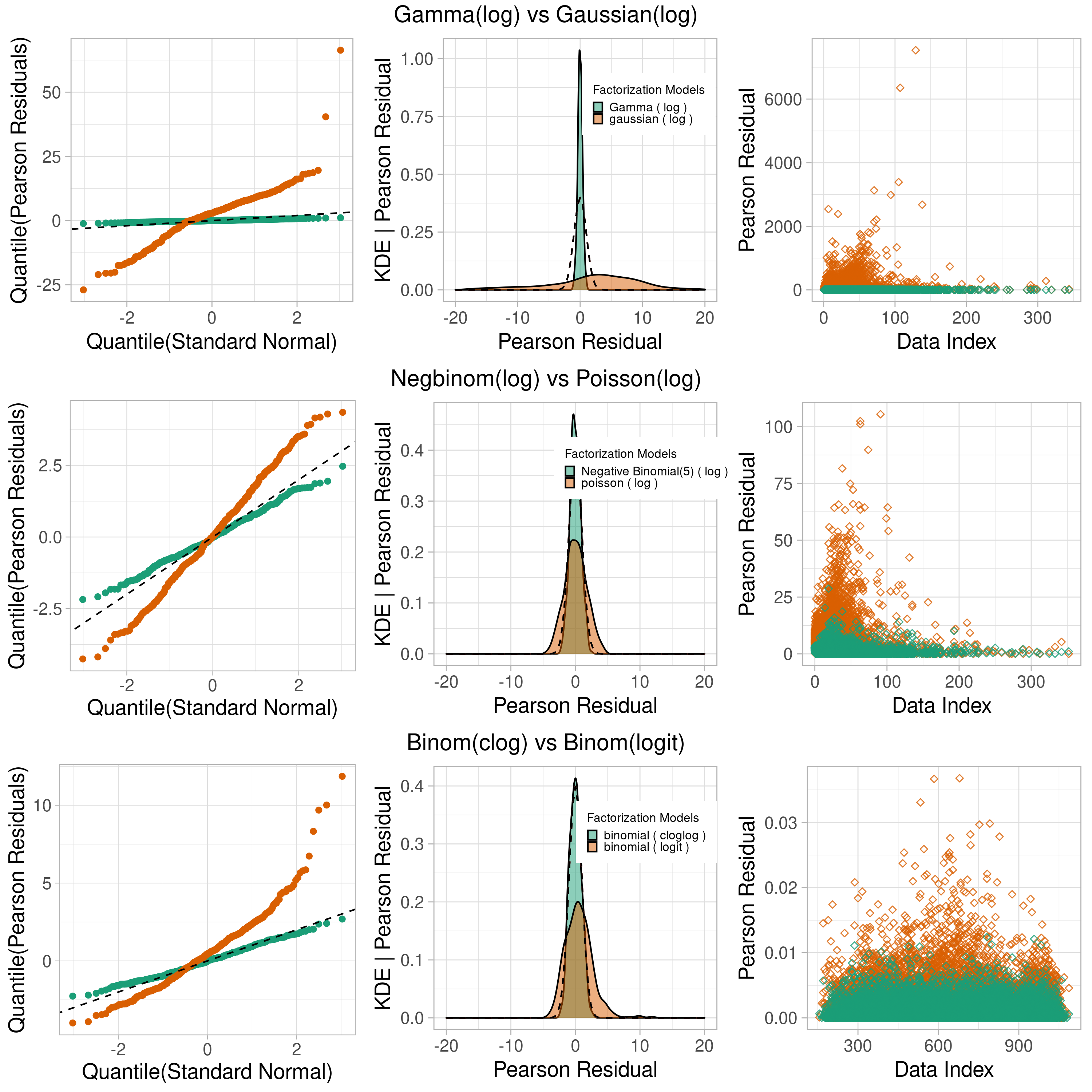
Figure 1: Goodness of fit tests: green indicates matched family/link fits. Columns (from left to right) represent respectively the QQ, density, and Pearson residual plots.

By comparing Pearson residuals (third column in Figure 1), we can conclude that a DMF under correct family and link parameterizations indeed yields better results. Since we generate the data from the given family (in green), it is not surprising to observe that all $\chi^{2}_{G-1}$ test statistics from correct family/link specifications have p-values equal to 1 and all $\chi^{2}_{G-1}$ statistics from wrong family/link assumptions have p-values equal to 0.

Notice that for the family test in Figure 1 we employed the gamma and negative binomial families with true dispersion parameter $\phi$, which is unknown in real world datasets. We here suggest that a naive moment estimator of the dispersion estimator (e.g., $\widehat{\phi}=\text{max}\{0.1,\mu_{X^{2}}/(\sigma_{X}^{2}-\mu_{X})\}$ for negative binomial) can still effectively distinguish the true simulation factorization family from the comparing non-dispersed factorization family. With the same $q,p,n$ and $\Lambda_{0},V_{0}^{\top}$ setup, we simulate gamma and negative binomial data and compare $\chi^{2}$ family test p-values among three different factorization families: 1) dispersed family with true dispersion $\phi$, 2) dispersed family with estimated dispersion $\widehat{\phi}$, and 3) non-dispersed family. We generate data matrices and evaluate family test p-values for 10,000 simulations. The results from a Poisson-negative binomial example are shown in Figure 2.

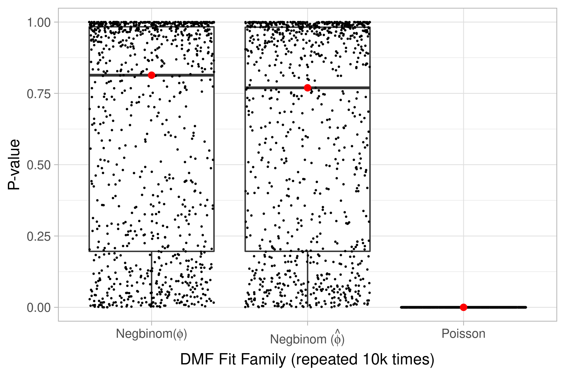
Figure 2: Sensitivity analysis on $\phi$ estimation: with red dot indicating the median, all simulations are under log link.

From Figure 2, we can conclude that the p-values are not significantly different when we compare between estimated and true dispersion parameters in factorizations for dispersed families. Both dispersed factorizations are clearly different from the Poisson factorization family. The high p-values for the dispersed families indicate that there is no sufficient evidence to reject the null hypothesis that the negative binomial (dispersed family) is the true factorization family. In fact, because the negative binomial distribution is more flexible and better represents the variance in data entries, it should consistently show higher p-values when compared to the Poisson distribution even when the data already show good agreement with the non-dispersed (Poisson) family. We have empirically confirmed this observation in a separate simulation study.

5.1.2 Power Analysis

We investigate the power of our test according to two sets of parameters: $n$ and $p$, specifying the sample size; and $\|\eta\|_{F}$, controlling the effect size. Power is, in general, sensitive to these parameters, increasing with them. However, in our setup we expect a more complex, combined effect: small data matrices with overall small entry magnitudes can be well explained by multiple families, while larger matrices provide more opportunities to spot discrepant entries under the null, specially with larger entries as they impact the variance function $\mathcal{V}$ more pronouncedly.

Since deriving the power of the test analytically is challenging under the DMF setup, we estimate it empirically under four commonly used factorization families in simulation studies. The four selected factorization families and links are poisson (log), binomial (logit) with weight $w=90$, gamma (log) with $\phi=1$, and negative binomial (log) with $\phi=5$. For each combination of factorization family and link, we simulate data under $n=200$, $600$ and vary the dimension according to $p=[0.2n,0.3n,\ldots,0.7n]$. The magnitude $\|\eta\|_{F}$ is controlled by a $\sigma$ parameter with $\eta_{ij}=\Lambda_{i}^{\top}V_{j},\Lambda_{i}\sim N(0,\sigma^{2}I_{q}),V_{j}\sim N(0,\sigma^{2}I_{q})$. The $\sigma$ parameter is taken to be $\{0.1,0.2,0.3,0.4\}$ for the four families.

We simulate data $X$ according to each of the four families indexed by $j=1,\ldots,4$ under each $n,p,\sigma$ setup. The simulation(sampling) is repeated $S=30$ for each of the family index. Conditional on each of the simulated data $X$, we then choose $G=np/50$ to ensure each group has $50$ residual observations. Next, we compute the p-value for the generalized Hosmer-Lemeshow test using each of these four families indexed by $i=1,\ldots,4$ as the null family, with $i=j$ indicating a DMF fit under the true generating family/link assumption. For each combination of simulated hypothesis family $j$ and fitted hypothesis family $i$, we denote as $P_{s}(i,j)$ the $p$-value for sample $s$. This simulation provides power estimates $1-\widehat{\beta}(i,j)=\frac{1}{S}\sum_{s=1}^{S}1(P_{s}(i,j)\leq\alpha)$ at significance level $\alpha$ whenever $i\neq j$. In the study we set $\alpha=0.05$. As an initial sanity check, the power of two extreme cases of $n,p,\sigma$ are shown in Figure 3.

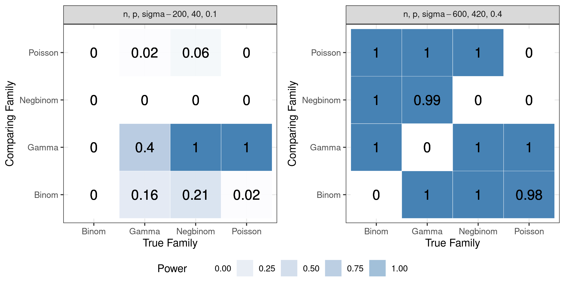
Figure 3: Extreme power comparison.

As we can see from the left matrix in Figure 3, in general, with small sample sizes ($n=200$, $p=40$) and magnitude ($\sigma=0.1$) we have low power as expected, shown here by having $1-\widehat{\beta}(i,j)\approx 0$ on the off-diagonal elements. True dispersed families such as gamma and negative binomial, however, show better discriminatory power even at these challenging conditions. As we focus on the right figure to increase sample sizes $n,p$ and the effect size $\sigma$, we observe higher power, again as expected. The only exception to $1-\widehat{\beta}(i,j)\approx 1$ in the off-diagonal entries in the right matrix is the true Poisson versus compared negative binomial case, which is also expected since the former is a particular case of the later. This observation additionally confirms the robustness of the negative binomial distribution in terms of explaining variation within Poisson data.

Despite the fact that the designed statistics is able to distinguish the correct families and links, we observe that the diagonal of the two matrices in Figure 3 is not converging to the advertised $\alpha=0.05$ significance level. From our empirical explorations, the desired $\alpha=0.05$ convergence can be achieved by requiring 1) asymptotically larger $n$, $p$, 2) a carefully chosen number of groups $G$ and 3) a good initialization point for optimization convergence. The consideration of these factors will further depend on the family and link being simulated, which will make the design of the experiment unnecessarily lengthy. We decided to keep this interest open to follow-up research since this experiment has sufficiently provided the first assurance (to the best of our knowledge) for practitioners to access the appropriateness of the DMF family/link. That is, the experiments designed here clearly demonstrate that the test has high sensitivity and specificity with large sample sizes.

Next, to observe the effect of size on power, we estimate it from 10 replicates under different simulation scenarios of increasing $n\times p$ overall size with fixed $\sigma=0.4$. The results are summarized in Figure 4. As we can see, the power of our family test generally increases as the sample size $np$ increases while keeping the nominal significance level. As in the previous simulation study, negative binomial fitted models fail to reject Poisson data, as expected. Interestingly, negative binomial generated data is harder to fit under other families, even dispersed ones, while Poisson generated data is more flexible and be well fit even with a binomial family under a low sample size.

Figure 4: Sample size effect on the power of family test.

Lastly, we are also interested in the impact of $\|\eta\|_{F}$ through the parameter $\sigma$. In Figure 5 we plot how power varies as a function of $\sigma$ for fixed $n=200$ and $p=80$ over 10 replicates. As expected, power increases monotonically with the magnitude $\sigma$, indicating a clear effect of $\|\eta\|_{F}$ in distinguishing the variance structure and thus providing effective family selection.

Figure 5: Sigma effect on the power of family test.

5.2 Rank Simulation Study

To determine the effectiveness of factorization rank estimation, we continued to simulate data given a specific family and link function $X\sim F(g^{-1}(\eta))$, where $\eta=\Lambda_{0}V_{0}^{\top}+\Lambda V^{\top}$ is of a known true rank $q^{*}$. To test and compare the generality and the accuracy of two possible rank estimation methods [Adjust Correlation Threshold, ACT; 12] and [38]’s maximum eigenvalue gap, we generate both random and deterministic $\Lambda$ and $V$ according to the conditions in our Theorem 4.1 and Proposition 4.3.

For the implementation of the ACT method, we simply take $\widehat{\eta}=g(X)$ and use the Stieltjes transformation on the eigenvalues of its correlation matrix. For the maximum eigenvalue gap method, we simply adopt the $\delta$ calibration algorithm in [38] with $q_{\text{max}}=p-5$. For each simulation scenario, we set $p=50$, $n=500$, and vary the true rank $q^{*}$. We set $\Lambda_{0}V_{0}^{\top}=\mathbf{5}_{n\times p}$ to maintain the linear predictor positive, as required for the gamma, Poisson, and negative binomial distributions, but set $\Lambda_{0}V_{0}^{\top}=\mathbf{0}_{n\times p}$ to avoid perfect separation in the binomial case. Here we highlight a simulation scenario with $n=500$ and $p=50$; experiments under different aspect ratios $p/q\in[0.1,0.2,\cdots 1]$ are repeated and resulted in similar conclusions, so they are not shown for brevity. We simulate the rank determination process 1,000 times under the different scenarios listed in Table 3.

Table 3: Rank simulation cases.

	$q^{*}$	$\Lambda$	$V$
Case 1	6	$\Lambda_{ij}\sim N(0,1)$	$V_{ij}\sim N(0,1)$
Case 2	6	$\Lambda_{ij}\sim\text{Unif}(-n/50,n/50)$	$V=[\text{Diag}(1)_{q\times q}|0_{q\times(p-q)}]$
Case 3	15	$\Lambda_{ij}\sim N(0,1)$	$V_{ij}\sim N(0,1)$
Case 4	15	$\Lambda_{ij}\sim\text{Unif}(-n/50,n/50)$	$V=[\text{Diag}(1)_{q\times q}|0_{q\times(p-q)}]$
Case 5	6	$\Lambda_{ij}\sim N(0,\sigma=0.1)$	$V_{ij}\sim N(0,\sigma=0.1)$
Case 6	6	$\Lambda_{ij}\sim\text{Unif}(-0.1,0.1)$	$V=[\text{Diag}(1)_{q\times q}|0_{q\times(p-q)}]$

Case 1 was designed with both the conditions of ACT and maximum eigenvalue gap method in our Proposition 4.3 satisfied. Case 2 was conducted with the true $V$ matrix being deterministic, which is permitted in Proposition 4.3 but violates the assumption in the ACT method. Cases 3 and 4 were designed with $q^{*}$ relatively large compared to data dimension $p$, which violates the assumption of $q^{*}=O(p^{\delta})$ in ACT methods for $\delta$ large. Cases 5 and 6 are designed to demonstrate the failure of both methods in the case of weak signal (condition C1 in Theorem 4.1 is violated). The simulation results are shown in Figure 6.

Figure 6: Rank simulation results: ACT (red), maximum eigenvalue gap (blue).

We can conclude that although the ACT method works almost perfectly when the conditions in [12] are satisfied, it also consistently fails to estimate the true rank when the conditions are violated (e.g., in case 2 with $V$ being deterministic, case 3 when $q^{*}$ is relatively large compared to $p$). On the other hand, the maximum eigenvalue gap method estimates the true rank $q^{*}$ with few mistakes for the first four simulation scenarios.

If we take a closer look at the maximum eigenvalue gap plot we notice that most, if not all, of the over estimations resulting from the maximum eigenvalue gap method are caused by the crude $\delta$ calibration algorithm in [38]. That is, the algorithm attempts to capture the maximum eigenvalue gap through estimating the slope locally up to convergence, which might suffer from high variance under a limited local data sample. A typical overestimating effect is shown in Figure 7, which clearly indicates a rank 6 and 15 but the $\delta$ calibration algorithm outputted a rank of 9 and 17 for cases 2 and 4.

Figure 7: Negative binomial rank overestimation.

We thus encourage the user to always plot the eigenvalue gap to supervise the determination of factorization rank. We also refer to Onatski’s $\delta$ calibration algorithm for a potential improvement on the automatic algorithm robustness. In conclusion, we adopt the maximum eigenvalue gap method for rank determination in our empirical data study as it is more flexible and robust.

5.3 Case Studies – Visualization

5.3.1 Face Recognition

Since pattern recognition is closely related to matrix factorization, we tried our method on a computer vision benchmark dataset. The CBCL dataset is a two class dataset with 2,429 of them being human faces and 4,548 images being non-face images. Enriched with followup research, the CBCL dataset has been extensively employed in computer vision research [6]. Containing the first comparison among PCA, NMF and factor model on the CBCL dataset, the work of [30] brought considerable attention to NMF in computer vision.

Here we compare factorization results of the CBCL dataset with four potential factorization families: 1) the constrained Poisson identity link (NMF), 2) the unconstrained Poisson log, 3) the negative binomial log with MoM-estimated $\widehat{\phi}=0.462$, and 4) the binomial family probit link with weights as 255 (max grayscale value in dataset images). The binomial factorization with weight 255 is particularly interesting because it offers the statistical view of computer images as binomial allocations.

We first determine the factorization rank by fitting $\widehat{\eta}$ with a full rank ($q=361$) and by performing the maximum eigenvalue gap method (with $q_{max}=30$). The results indicate a rank of three for negative binomial, Poisson (log link), and binomial, and a rank of four for Poisson (identity link, NMF). Eigenvalue plots can be found in Appendix A. We then perform the family test with $G=165$ with results shown in Figure 8.

Figure 8: CBCL factorization family test with $G=165$. QQ-plot (left), density plot (right). Both are overlaid with a standard normal density (black dashed line).

As can be seen, the negative binomial family is closest to normality on its components $T_{n,p}^{1}(D_{n,p}^{1})^{\frac{1}{2}}$ and thus the highest p-value in $\chi^{2}_{G-1}$ statistics. It is then followed by the binomial with probit link, NMF, and log-link Poisson. Note that even though the negative binomial factorization family is the best among the four potential families, we still observe tail deviations from the $45\deg$ line in the QQ-plot. We attribute this deviation to the unusual presence of zeros as the background color. The tail deviation thus points out to a potential factorization research direction with the generation of background pixels being modeled by a separate specification as in zero-inflated models.

Next, we compare the projected three dimensional $\widehat{\Lambda}$ for these four families, as shown in Figure 9. Even though the negative binomial factorization family is the best among the four in the family test, the projected three dimensional plot indicates better separability between the face and non-face classes under the NMF factorization. This result suggests a better fit of negative binomial and binomial factorization to the image data by better accommodating the dispersion induced from different classes, but a less clear separability between faces and non-faces. This observation is related to the positivity constraint imposed by the NMF method, which has been shown in [30] to promote partial face learning. A potential research direction thus would be to fit DMFs under a classification scenario, for instance, a negative binomial or binomial family factorization for faces and non-faces, with different factors $\Lambda$ and $V$ for each class.

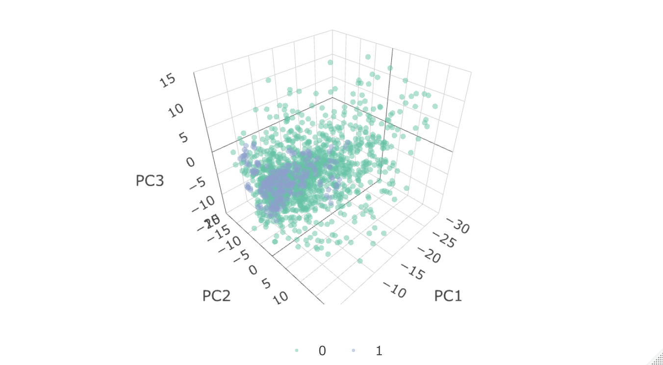
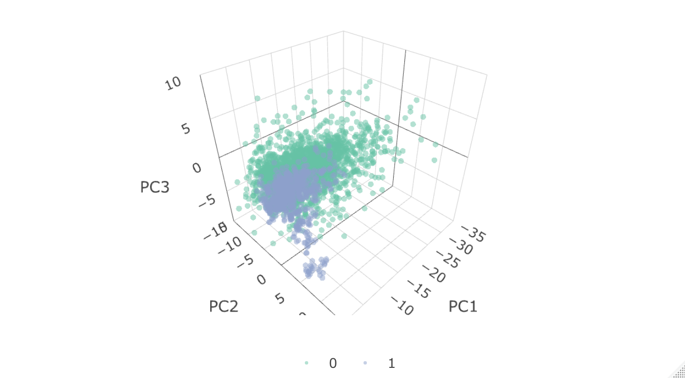
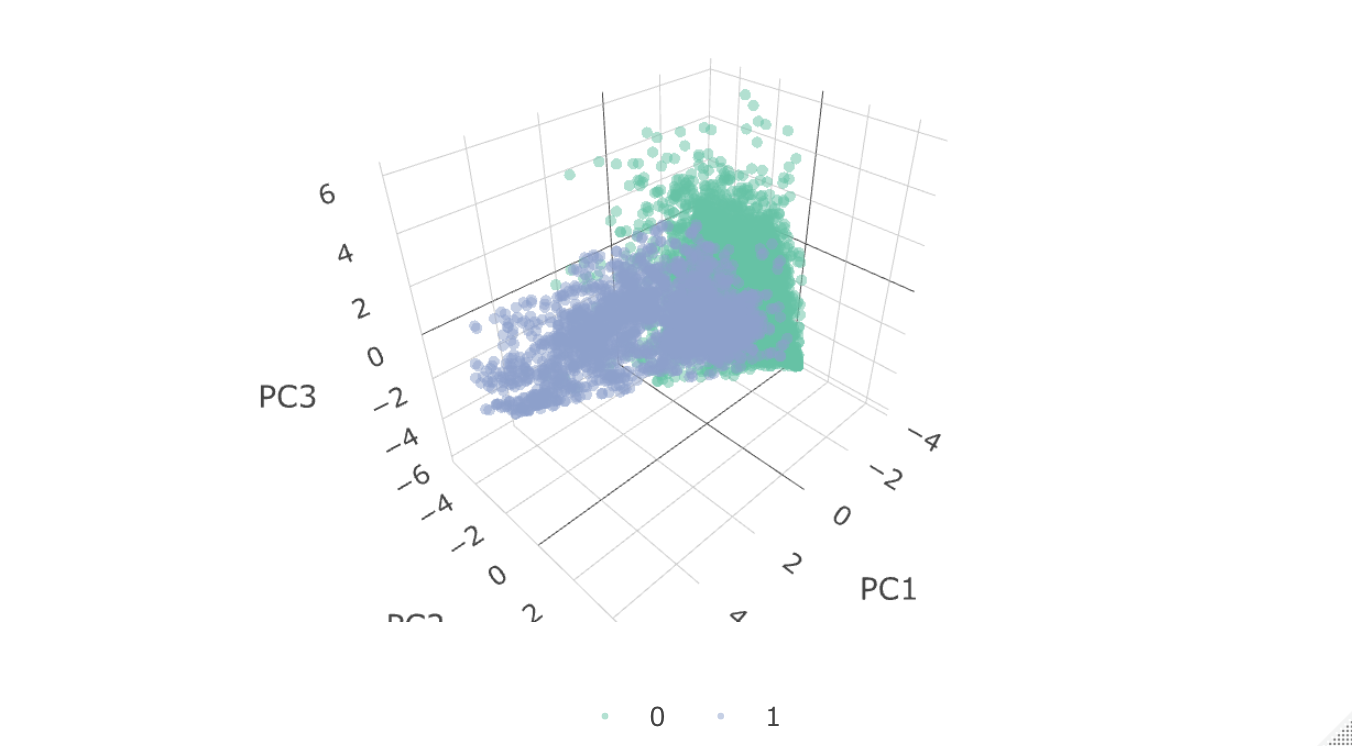
Figure 9: CBCL factorization projections: negative binomial (top left), Poisson (top right), binomial (bottom left), and NMF (bottom right).

5.3.2 Natural Language Processing

Besides applications in computer vision, natural language processing (NLP) has also been a very successful application area for matrix factorization. The factorization is usually based upon a keyword co-occurrence matrix, then termed as latent semantic analysis [LSA; 10], or keyword-document matrix, known as hyperspace analogue to language [HAL; 34]. One recent breakthrough is GloVe [24], which motivates the use of a log link on the probability of word co-occurrence matrix for word analogy task.

We hereby compare the NMF factorization against our DMF factorization with negative binomial and Poisson log links by experimenting on one of the NLP benchmark datasets known as “20Newsgroup”[29]. The dataset contains 20,000 articles with each of them associated with one of 20 news topics. For visualization convenience, we focus on four topics—auto, electronics, basketball, mac.hardware—that are different enough and can adopt similar preprocessing methods to [17]. Specifically, to avoid overfitting on specific documents, we filtered out the headers and footers and quote information within the news while tokenizing specific keywords using English stop words. For the tokenization of the keywords, we also filter out words that show up in 95% of the articles and keywords that appear in only one article to promote the effectiveness of keyword identification. After preprocessing, we end up with 3,784 documents and 1,000 keywords. We use the frequency matrix as the input of our matrix factorization with $n=3,784$ and $p=1,000$.

Since the data is a positive count matrix, we here compare the factorization results of NMF, Poisson log and negative binomial with MoM-estimated $\widehat{\phi}=0.06$. For both the Poisson log and negative binomial log family we have found a rank of $\widehat{q}=5$, while for the NMF we have $\widehat{q}=3$. To better visualize factorization results, we adopt a factorization with $\widehat{q}=3$ for all the families to ensure a fair comparison to NMF. We then conduct a family test with $G=20$ in Figure 10.

Figure 10: Keyword frequency factorization family test: $G=20$,QQ-plot (left), density plot (right). Both are overlaid with a standard normal density (black dashed line).

With a unit p-value, we take the negative binomial family with log link and MoM-estimated dispersion ($\widehat{\phi}=0.06$) as an adequate distribution while rejecting the Poisson family with log link and NMF with Poisson identity link with both of them having zero p-value.

Lastly, we adopt (7) for all the three factorization to better visualize the projected three dimensional plot in Figure 11. We can see after projecting the 3,784 documents onto the three dimensional factor space, the negative binomial factorization more clearly separates the four different topic classes. Compared to the negative binomial factorization, the Poisson log factorization can still separate the four different class albeit in a more compact way, which suggests the indispensability of dispersion to account for keyword frequency variation. The NMF with Poisson identity link perform the worst, with four topics overlapping in the center, at the origin.

Figure 11: Keyword frequency factorization projection: negative binomial (left), Poisson (center), and NMF (right).

5.3.3 Network Analysis

Another important application of our deviance matrix factorization is network data analysis, and here we focus on community detection [13]. Since the adjacency matrix of a network has binary entries, we can just adopt a Bernoulli family for the factorization. To demonstrate the effectiveness of our DMF method on network data, we use the political blogs and Zachary’s karate club datasets as examples, both of which have been benchmark datasets for network community detection since [13] and [1].

We thus just compare the binomial logit link factorization with the commonly used Laplacian spectral clustering method and use the separation of projected principal components in $\widehat{\Lambda}$ to assign communities.

As before, we first employ maximum eigenvalue gap method to determine the factorization rank. With $q_{max}=200$ and $q_{\text{max}}=29$, we have found rank three to be true factorization rank for political blogs and a rank two for karate club network (see Figure 19). The projected two dimensional plot in Figure 12 suggests good separation between two groups, with the leaders being far from the centroid of their respective groups. Notice that both methods can identify two communities with a single principal component, but the DMF method provides more information about group variations in the second principal component.

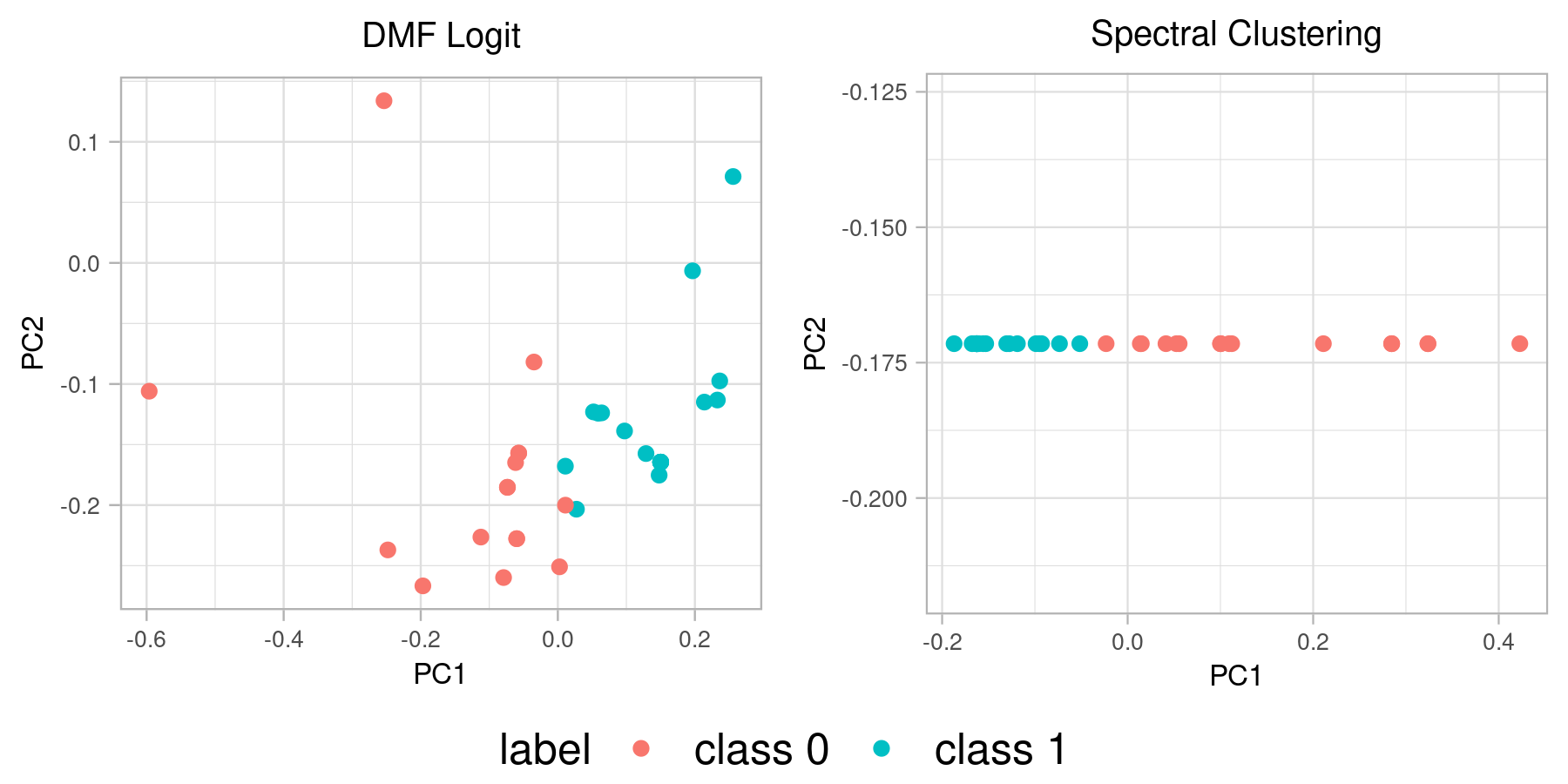
Figure 12: Karate club factorization projections.

Although our method can take asymmetric and undirected network data as inputs for the factorization, the Laplacian clustering method depends heavily on the positive definite property of a connected symmetric graph. To ensure a fair comparison between our method and Laplacian clustering, we pre-process the data by focusing on the largest connected component, which consists of 1,222 nodes. As the projected three dimensional plot in Figure 13 indicates, compared to the spectral clustering method our method has a much clearer separation across the two known communities and better captures within group variation by exploiting all three factorized principal components.

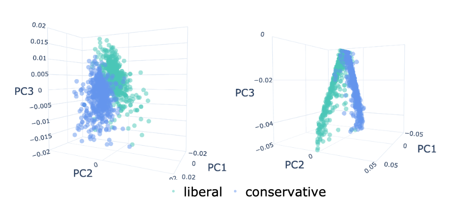
Figure 13: Polblog factorization projections: binomial logit (left), spectral clustering (right)

5.3.4 Biomedical studies

The leukemia dataset reported in [15] has been a staple benchmark for gene classification. The dataset contains 5,000 features and 38 observations with two known labels of classes: acute myelogenous leukemia (AML) and acute lymphoblastic leukemia (ALL). Recent researches [5, 54] have explored factorizations based on PCA and NMF with ranks ranging from 2 to 5.

For similar dispersion reasons, we compare factorization results among NMF, Poisson with log link, and negative binomial with $\widehat{\phi}=1.93$. Similar to the previous experiments, we first employed the maximum eigenvalue gap method with a full rank fit to determine the factorization rank. The results indicates a rank two factorization for negative binomial with log link and a rank one for the Poisson log-link model. For the NMF rank determination, we adopt the similar procedure by fitting the NMF with full rank and then plot the maximum eigenvalue gap. The results indicate possible ranks of two and possible rank of four for the NMF (Poisson with identity link) factorization.

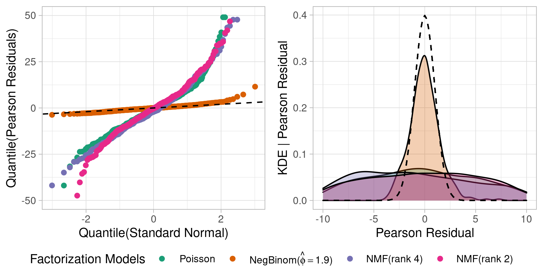
Figure 14: Leukemia factorization family test: with $G=380$, QQ-plot (left), density plot (right). Both are overlaid with a standard normal density (black dashed line).

We then conduct the family test to determine the appropriate factorization family, as shown in Figure 14. We can see that Poisson (log), NMF, and PCA (identity) all failed the normality test, while the negative binomial family with log link demonstrates significant better normality. This result justifies a negative binomial family with log link as a reasonable factorization family.

Figure 15: Leukemia dataset factorization projections.

Lastly, we compare the factorized projected matrix $\widehat{V}$ in Figure 15. Since in this particular factorization the three different families all have different ranks, we plot the projected $\widehat{V}$ along sample indices with leukemia types (ALL versus AML) separated by a vertical line. As Figure 15 shows, the negative binomial family with log link can correctly distinguish the two types by using just two principal components. In contrast, the non-negative matrix factorization gives spurious results even with a higher factorization rank. The rank two factorization result for NMF is better compared to NMF rank four factorization, but the sample types are not as well separated as in the negative binomial factorization, especially for samples 6, 17, and 29. Thus we conclude that the NMF (Poisson with identity link) and Poisson family (with log link) are not capturing the essential information of the matrix completely; for instance, the factorized principal scores could not effectively distinguish the correct types. By better taking data dispersion into consideration, the negative binomial factorization is in general better suited for positive count gene data factorizations.

5.4 Case Studies – Classification

In the previous case studies we observe notable separability even from DMFs of low ranks of $2$ and $3$ when compared to other benchmark methods. Here we aim to further quantify this separability with objective downstream classification tasks. We conducted these comparisons under three inherently different classification models—tree, multinomial regression and k-nearest neighbors (KNN) with $k=9$—using 20 factorized components. For each classification model we replicated training/testing for 10 runs with equal split on training (50%) and on testing (50%). Performances are summarized using boxplots on the 10 reproduced multi-class AUC [19], which has been shown to be invariant to class-skewness.

Figure 16: Multi-class AUC comparison.

As we can see from Figure 16, the DMF model has better performance in all the three classification models for the NLP dataset and for the polblog dataset. Perhaps due to a limited sample size (38 labels for leukemia), the performance for the leukemia dataset varies significantly on the classification model being used but overall we see that the DMF and NMF perform similarly with 20 PCs. For the CBCL face/non-face dataset, we see that the NMF model performs the best using multinomial regression and tree classification. However, both of the two methods are less-desired compared to KNN, achieving a nearly perfect score for the binomial DMF.

6 Conclusion

We have proposed a new approach for matrix factorization. The factorization method generalizes the commonly applied PCA and NMF methods to accommodate more general statistical families that take data features such as over dispersion into consideration. To this end, we have generalized a fitting algorithm with convergence to at least a stationary point being justified, and have provided methods, supported by theoretical guarantees, to determine factorization family and rank.

We also obtained encouraging experimental results in our simulated data studies and in many case studies using benchmark datasets from different fields. As we show in Section 5, our method can better explain sparsity patterns in keyword frequency and gene expression matrices through over-dispersed families such as the negative binomial. It also provides an alternative factorization perspective to image recognition by changing the original problem to an optimal binomial weights allocation problem. It further enriches community detection research in network analysis by allowing a general factorization method that is applicable to asymmetric and weighted networks.

Our work offers an important perspective to matrix statistical inference by extending the probability concept from Gaussian and Poisson to more general exponential families with different link functions. In fact, we plan to explore zero inflated models to improve fit and interpretability in face of matrices with excess zeros. For future research, we intend to enrich our deviance matrix factorization with a hierarchical structure to model matrix mixtures to effectively incorporate row or column classification and to investigate more efficient optimization procedures for very large datasets.

7 Acknowledgement

We thank two anonymous referees and the associate editor who provided many valuable comments that significantly improved the paper. We also thank Weixuan Xia who provided suggestions and validation on our consistency proof.

Appendix A Factorization Ranks

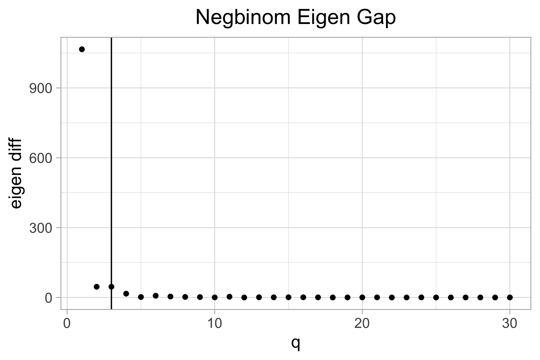
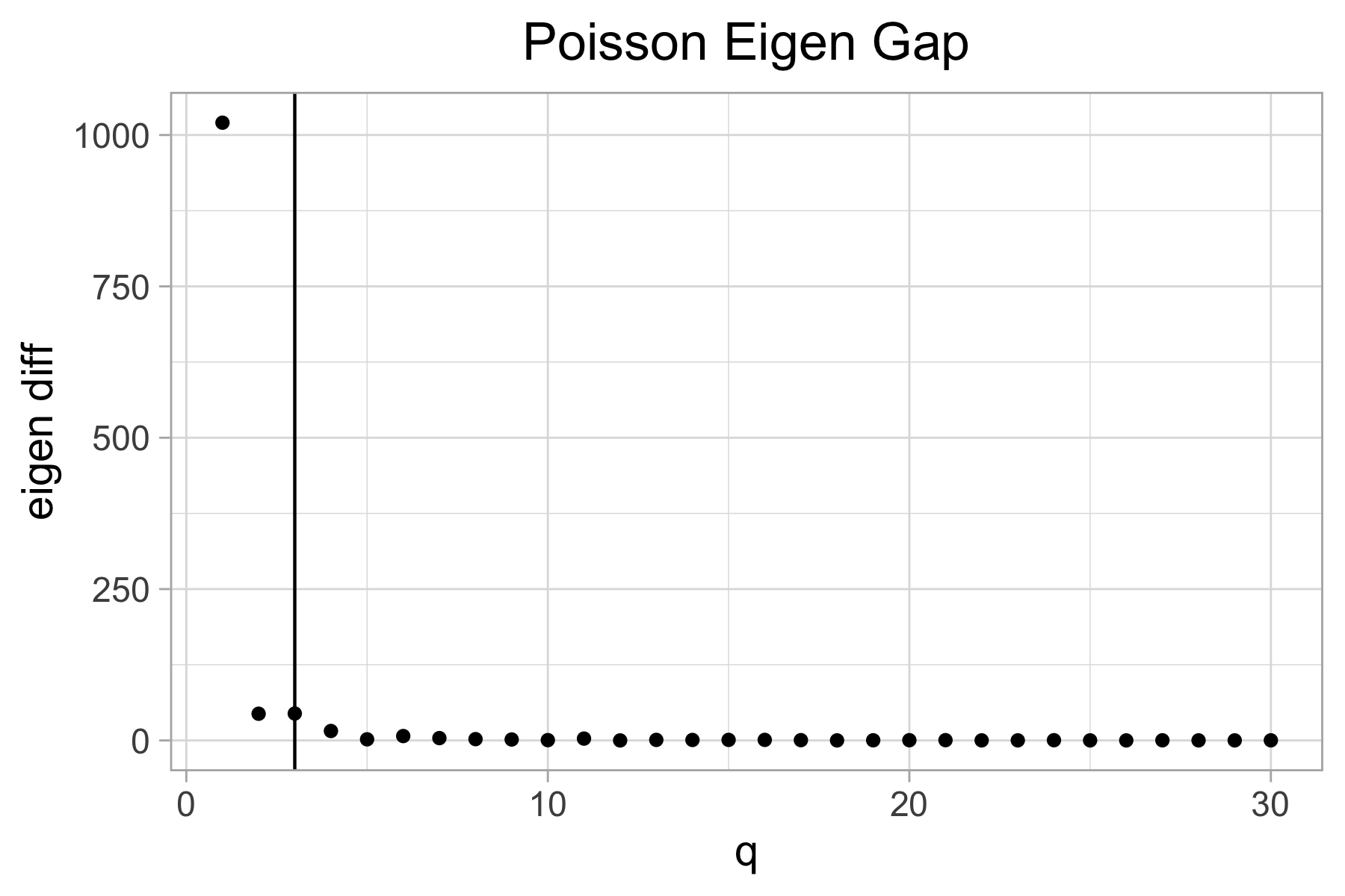
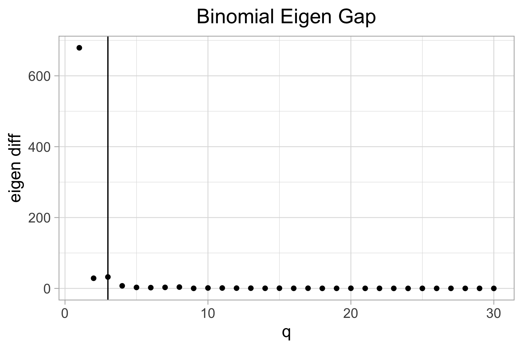
Figure 17: CBCL factorization eigengap.

Figure 18: Keyword frequency factorization eigengap.

Figure 19: Network factorization eigengap.

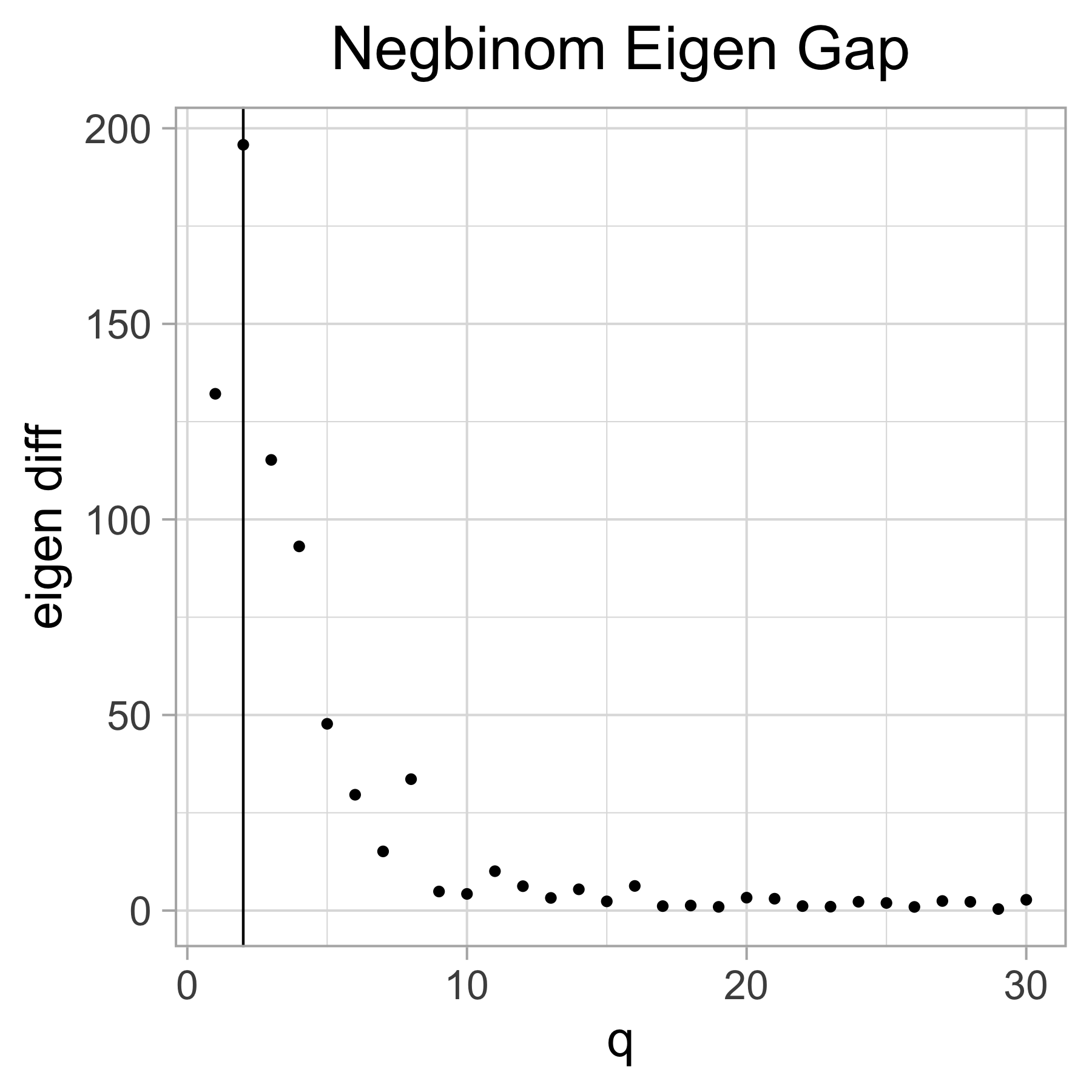
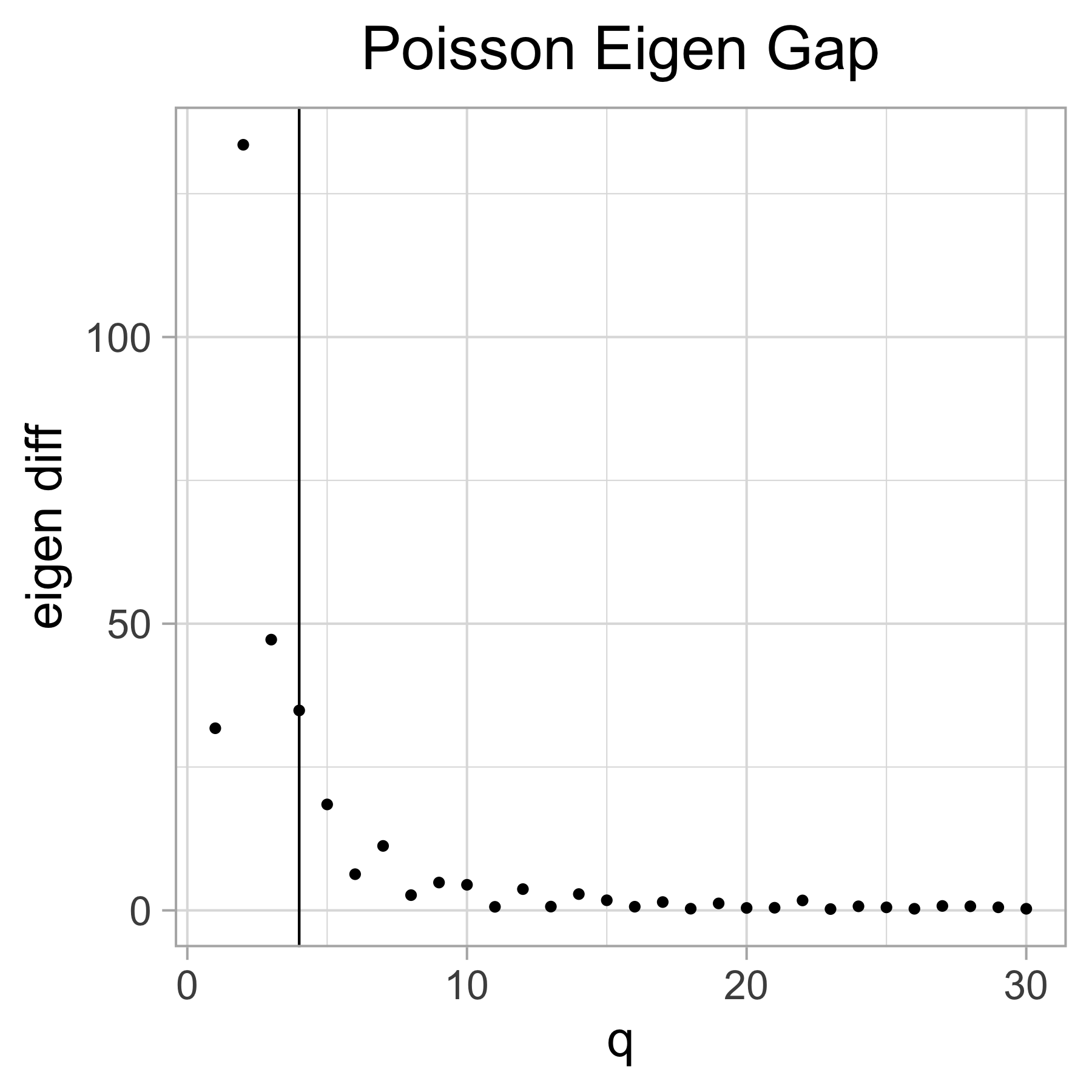
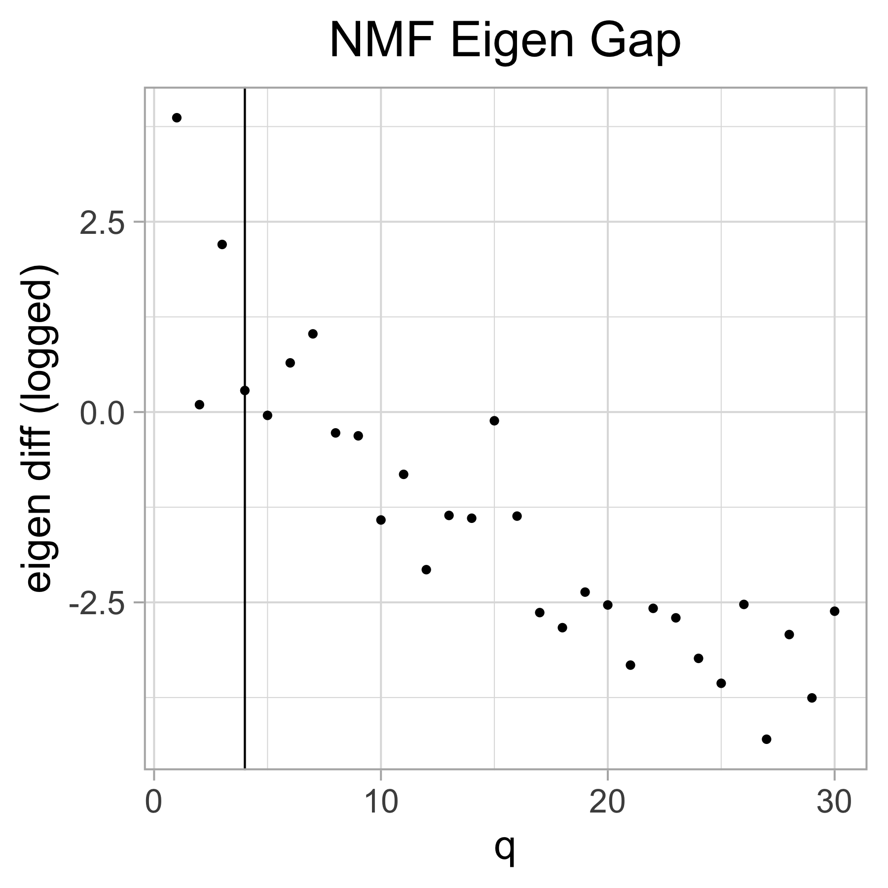
Figure 20: Leukemia factorization eigengap.

Appendix B Theoretical Guarantees

B.1 Proof of Theorem 4.1

The consistency proof is based upon Theorem 1 in [8] with some additional inequalities being imposed. We start with the following lemma:

Lemma B.1.

For smooth injection mapping $H(\cdot):\mathbb{R}^{q}\rightarrow\mathbb{R}^{q}$ with $H(x_{0})=y_{0}$. Define $B_{\delta}(x_{0})=\{x\in\mathbb{R}^{q},\|x-x_{0}\|_{2}\leq\delta\}$ and $S_{\delta}(x_{0})=\{x\in\mathbb{R}^{q},\|x-x_{0}\|_{2}=\delta\}$, then $\inf_{x\in S_{\delta}(x_{0})}\|H(x)-y_{0}\|_{2}\geq r$ implies:

• $B_{r}(y_{0})\subseteq H(B_{\delta}(x_{0}))$

• $H^{-1}(B_{r}(y_{0}))\subseteq B_{\delta}(x_{0})$

Proof.

The proof is detailed in the appendix of [8]. ∎

B.1.1 The first order conditions

Denote $\eta_{ij}=\Lambda_{i}^{\top}V_{j}$ where $\Lambda_{i}$ is the i-th row of factorized matrix $\Lambda$, $V_{j}^{\top}$ is the j-th column of factorized matrix $V^{\top}$. As a notational convention, all vectors are defined as column vectors with their inner products being scalar. Under an exponential GLM setup, the log likelihood with parameter of interest $\theta_{ij}=\theta(\eta_{ij})$, dispersion parameter $a(\phi)$, mean function $\mu_{ij}=m(\eta_{ij})$ and cumulant function $b_{ij}=b(\eta_{ij})$ could be written in the following form:

$$l(\Lambda,V) =\sum_{i=1}^{n}\sum_{j=1}^{p}l(\Lambda_{i}^{\top}V_{j})$$ (18)

$$=\sum_{i=1}^{n}\sum_{j=1}^{p}\frac{1}{a(\phi)}(X_{ij}\theta_{ij}-b(\theta_{ij})+c(X_{ij},\phi))$$

After convergence of Algorithm 1, denote $l_{ij}=l(\eta_{ij})$. We will have the following first order condition to be satisfied:

$$\frac{\partial l(\Lambda,V)}{\partial V_{j}^{\top}} =\sum_{i=1}^{n}\frac{\partial l_{ij}}{\partial\theta_{ij}}\frac{\partial\theta_{ij}}{\partial\mu_{ij}}\frac{\partial\mu_{ij}}{\partial\eta_{ij}}\frac{\partial\eta_{ij}}{\partial V_{j}}=\mathbf{0}_{q}$$ (19)

$$\frac{\partial l(\Lambda,V)}{\partial\Lambda_{i}} =\sum_{j=1}^{p}\frac{\partial l_{ij}}{\partial\theta_{ij}}\frac{\partial\theta_{ij}}{\partial\mu_{ij}}\frac{\partial\mu_{ij}}{\partial\eta_{ij}}\frac{\partial\eta_{ij}}{\partial\Lambda_{i}}=\mathbf{0}_{q}$$

Specifically for the components, with $\mathcal{V}(\mu_{ij})$ being the variance function with mean $\mu_{ij}$ as the scalar input, we have:

$$\frac{\partial l_{ij}}{\partial\theta_{ij}} =\frac{1}{a(\phi)}(X_{ij}-b^{\prime}(\theta_{ij}))$$ (20)

$$\frac{\partial\theta_{ij}}{\partial\mu_{ij}} =(\frac{\partial\mu_{ij}}{\partial\theta_{ij}})^{-1}=\frac{1}{b^{\prime\prime}(\theta_{ij})}=\frac{1}{\mathcal{V}(\mu_{ij})}$$

$$\frac{\partial\mu_{ij}}{\partial\eta_{ij}} =(\frac{\partial\eta_{ij}}{\partial\mu_{ij}})^{-1}=\frac{1}{g^{\prime}(\eta_{ij})}$$

$$\frac{\partial\eta_{ij}}{\partial V_{j}^{\top}} =\Lambda_{i}^{\top},\quad\frac{\partial\eta_{ij}}{\partial\Lambda_{j}}=V_{j}^{\top}$$

Substituting into (19), we have:

$$\frac{\partial l(\Lambda,V)}{\partial V_{j}} =\sum_{i=1}^{n}\frac{1}{a(\phi)}(X_{ij}-b^{\prime}(\theta_{ij}))\frac{1}{\mathcal{V}(\mu_{ij})g^{\prime}(\mu_{ij})}\Lambda_{i}^{\top}=\mathbf{0}_{q}$$ (21)

$$\frac{\partial l(\Lambda,V)}{\partial\Lambda_{i}} =\sum_{i=j}^{p}\frac{1}{a(\phi)}(X_{ij}-b^{\prime}(\theta_{ij}))\frac{1}{\mathcal{V}(\mu_{ij})g^{\prime}(\mu_{ij})}V_{j}^{\top}=\mathbf{0}_{q}$$

Observe that $\theta_{ij}=\eta_{ij}$ under canonical link. Thus $g^{\prime}(\mu_{ij})=\frac{1}{\mathcal{V}(\mu_{ij})}$, which further gives us the normal equation from the least square estimation for fixed $\Lambda_{i}$ or $V_{j},\forall i=1...n,j=1...p$:

$$\frac{\partial l(\Lambda,V)}{\partial V_{j}} =\sum_{i=1}^{n}(X_{ij}-m(\Lambda_{i}^{\top}V_{j}))\Lambda_{i}^{\top}=\mathbf{0}_{q}$$ (22)

$$\frac{\partial l(\Lambda,V)}{\partial\Lambda_{i}} =\sum_{j=1}^{p}(X_{ij}-m(\Lambda_{i}^{\top}V_{j}))V_{j}^{\top}=\mathbf{0}_{q}$$

As we assume that there exist $\eta$ of rank $q$ that generates the data and maximize the likelihood, our DMF algorithm uses the data initialization to find the corresponding estimate $\widehat{\eta}$ as the global maximum of the likelihood. However, the solution of $(\Lambda,V)$ is still not unique up to a rotational matrix until we impose an identifiability constraints. In together with our identifiability constraints and the convexity of the exponential log-likelihood, we thus observe that $\widehat{\Lambda}_{i}$ is unique conditional on $\widehat{V}$ and that $\widehat{V}_{j}$ is unique conditional on $\widehat{\Lambda}$. At final algorithm convergence, our estimators are thus designed to maximize the likelihood and to satisfy the F.O.C in Eq (22):

$$(\widehat{\Lambda}^{\top}\widehat{\Lambda})^{-1}\sum_{i=1}^{n}\widehat{\Lambda}_{i}^{\top}(X_{ij}-m(\widehat{\Lambda}_{i}^{\top}\widehat{V}_{j})) =\mathbf{0}_{q}$$ (23)

$$(\widehat{V}^{\top}\widehat{V})^{-1}\sum_{j=1}^{p}\widehat{V}_{j}^{\top}(X_{ij}-m(\widehat{\Lambda}_{i}^{\top}\widehat{V}_{j})) =\mathbf{0}_{q}$$

B.1.2 Sketch of the proof

Intuitively speaking, if either $\widehat{\Lambda}$ or $\widehat{V}$ is known in Equation (23), the problem reduces to a multiple generalized linear regression model [8]. When both of the estimators are unknown, it is thus hopeful to put some constraints on the space of our estimators $\widehat{\Lambda},\widehat{V}$ such that the consistency is still attained. In this proof, we first demonstrate that by restricting the $L_{2}$ norm of estimator $V$ with the orthogonal design ($\widehat{V}^{\top}\widehat{V}=I_{q}$), the estimator of $\widehat{\Lambda}_{i},\forall i=1,\cdots,n$ is strongly consistent. After which, we can derive the consistency property of estimator $\widehat{V}_{j},\forall j=1,\cdots,p$ in a similar manner.
We start by defining an auxiliary $q$ by $1$ vector $\widetilde{G}(\cdot):\mathbb{R}^{q}\rightarrow\mathbb{R}^{q}$

$$\widetilde{G}_{\widehat{\Lambda}_{n}}(\widehat{V}_{j}) =(\widehat{\Lambda}^{\top}\widehat{\Lambda})^{-1}\sum_{i=1}^{n}\widehat{\Lambda}_{i}^{\top}[m(\widehat{\Lambda}_{i}^{\top}\widehat{V}_{j})-m(\Lambda_{i}^{\top}V_{j})]$$ (24)

$$\widetilde{G}_{\widehat{V}_{p}}(\widehat{\Lambda}_{i}) =(\widehat{V}^{\top}\widehat{V})^{-1}\frac{1}{\sqrt{p}}\sum_{j=1}^{p}\widehat{V}_{j}[m(\widehat{\Lambda}_{i}^{\top}\widehat{V}_{j})-m(\Lambda_{i}^{\top}V_{j})]$$

Notice that the $\widetilde{G}_{\widehat{\Lambda}_{n}}(\widehat{V}_{j}),\widetilde{G}_{\widehat{V}_{p}}(\widehat{\Lambda}_{i})$ vectors are defined in a similar manner to the normal equation in Eq (23) with $X_{ij}$ changed to the expectation $m(\Lambda_{i}^{\top}V_{j})$. In a comparison to GLM setup that has either $\widehat{\Lambda}=\Lambda_{n}\in\mathbb{R}^{n\times q}$ or $\widehat{V}=V_{p}\in\mathbb{R}^{p\times q}$ fixed as observed data, [8] justified the consistency through some inequality relationship based upon the following vectors:

$$\widetilde{G}_{{\color[rgb]{1,0,0}\Lambda_{n}}}(\widehat{V}_{j}) =(\widehat{\Lambda}^{\top}\widehat{\Lambda})^{-1}\sum_{i=1}^{n}\widehat{\Lambda}_{i}^{\top}[m({\color[rgb]{1,0,0}\Lambda_{i}^{\top}}\widehat{V}_{j})-m(\Lambda_{i}^{\top}V_{j})]$$ (25)

$$\widetilde{G}_{{\color[rgb]{1,0,0}V_{p}}}(\widehat{\Lambda}_{i}) =(\widehat{V}^{\top}\widehat{V})^{-1}\frac{1}{\sqrt{p}}\sum_{j=1}^{p}\widehat{V}_{j}[m(\widehat{\Lambda}_{i}^{\top}{\color[rgb]{1,0,0}V_{j}})-m(\Lambda_{i}^{\top}V_{j})]$$

For the precise consistency inequality with $\widetilde{G}_{{\color[rgb]{1,0,0}V_{p}}}(\widehat{\Lambda}_{i})$ as an example,

$$\|\widetilde{G}_{{\color[rgb]{1,0,0}V_{p}}}(\widehat{\Lambda}_{i})\|_{2}^{2}\underbrace{\geq}_{{\color[rgb]{0,0,1}\text{Inequality}\ \ast}}\widetilde{Z}^{2}_{V_{\delta}}(\Lambda_{i})\|\Lambda_{i}-\widehat{\Lambda}_{i}\|_{2}^{2}$$

implies the following from Lemma B.1

$$\widehat{\Lambda}_{i}=\widetilde{G}^{-1}_{\widehat{V}_{p}}(\{b:\|b\|_{2}\leq Z^{2}_{V_{\delta}}(\Lambda_{i})\})\subseteq\{b:\|b-\Lambda_{i}\|_{2}\leq\delta_{\Lambda_{i}}\}$$

Our detailed proof then follows from building inequality relationship between Eq (24) and Eq (25). After which, consistency inequality in [8] can be readily applied. To facilitate the understanding, we focus on a summary on the proof in this section while postponing the inequality proof in Section B.1.3.

1). The Inequalities.

With $\|\cdot\|_{2}$ denote the spectral norm for matrix and euclidean norm(inner product) for vector, we will show that for large $p$, the following inequality holds true $\forall\ i=1,\cdots n$:

$$\|\widetilde{G}_{\widehat{V}_{p}}(\widehat{\Lambda}_{i})\|_{2}^{2}\underbrace{\geq}_{{\color[rgb]{0,0,1}\text{Inequality}\ \dagger}}\|\widetilde{G}_{{\color[rgb]{1,0,0}V_{p}}}(\widehat{\Lambda}_{i})\|_{2}^{2}\underbrace{\geq}_{{\color[rgb]{0,0,1}\text{Inequality}\ \ast}}\widetilde{Z}^{2}_{V_{\delta}}(\Lambda_{i})\|\Lambda_{i}-\widehat{\Lambda}_{i}\|_{2}^{2}$$

where $0<\widetilde{Z}_{V_{\delta}}(\Lambda_{i})<\infty$ is a positive and finite constant that introduced later in our detailed inequality proof. If the above inequality holds, we can readily apply Lemma B.1 to obtain:

$$\widehat{\Lambda}_{i}\in\widetilde{G}^{-1}_{\widehat{V}_{p}}(\{b:\|b\|_{2}\leq Z^{2}_{V_{\delta}}(\Lambda_{i})\})\subseteq\{b:\|b-\Lambda_{i}\|_{2}\leq\delta_{\Lambda_{i}}\}$$ (26)

where $\delta_{\Lambda_{i}}>0$ is an arbitrary small positive scalar. That is, we can find estimator $\widehat{\Lambda}_{i}$ as the pre-image of injection $\widetilde{G}_{\widehat{V}_{p}}(\cdot)$. The obtained estimator is sufficiently close to the true parameter $\Lambda_{i}$ with euclidean distance controlled by $\delta_{\Lambda_{i}}$.

2). The existence of $b\in\mathbb{R}^{q}$.

Based upon the definition of the fitted residual $e_{ij}=X_{ij}-m(\Lambda^{\top}_{i}V_{j})$, we can construct an $\mathbb{R}^{q}$ vector $a_{i}(\widehat{V}_{p})=\sum_{j=1}^{p}(\widehat{V}_{j}\widehat{V}_{j}^{\top})^{-1}\frac{1}{\sqrt{p}}\sum_{j=1}^{p}\widehat{V}_{j}e_{ij}$. By the result of our condition C2, we have

$$\lim\limits_{p\rightarrow\infty}a_{i}(\widehat{V}_{p})=\mathbf{0}_{q}\text{ a.s. }\forall i=1,\ldots,n$$

The result holds for arbitrary $n$. Consequently, for large $p$ and sufficiently small $\delta_{\Lambda_{i}}$

• $\widehat{\Lambda}_{i}=\widetilde{G}^{-1}_{\widehat{V}_{p}}(a_{i}(\widehat{V}_{p}))$ exists.

• $\widehat{\Lambda}_{i}=\widetilde{G}^{-1}_{\widehat{V}_{p}}(a_{i}(\widehat{V}_{p}))$ belong to $\{\Lambda_{i}:\|\widehat{\Lambda}_{i}-\Lambda_{i}\|_{2}\leq\delta_{\Lambda_{i}}\}$.

That is, the pre-image of $\widetilde{G}^{-1}_{\widehat{V}_{p}}(\cdot)$ with argument $a_{i}(\widehat{V}_{p})=\sum_{j=1}^{p}(\widehat{V}_{j}\widehat{V}_{j}^{\top})^{-1}\frac{1}{\sqrt{p}}\sum_{j=1}^{p}\widehat{V}_{j}e_{ij}$ is a consistent estimator as $p\rightarrow\infty$. The result again holds for all $i\in 1,\ldots,n$.

3). The relationship to the $\widehat{\Lambda}_{i}$ estimator

To justify that $\widehat{\Lambda}_{i}$ is uniquely our DMF estimator, we plug $\widehat{\Lambda}_{i}={\color[rgb]{1,0,0}\widetilde{G}^{-1}_{\widehat{V}_{p}}(a_{i}(\widehat{V}_{p}))}$ into the convergent condition of our estimator in Eq (23) with a harmless multiplication of $\frac{1}{\sqrt{p}}$.

$$(\widehat{V}^{\top}\widehat{V})^{-1}\sum_{j=1}^{p}\widehat{V}_{j}^{\top}(m({\color[rgb]{1,0,0}\widehat{\Lambda}_{i}^{\top}}\widehat{V}_{j})-X_{ij})$$ (27)

$$=\sum_{j=1}^{p}\widehat{V}_{j}^{\top}(m({\color[rgb]{1,0,0}\widetilde{G}^{-1}_{\widehat{V}_{p}}(a_{i}(\widehat{V}_{p}))^{\top}}\widehat{V}_{j})-X_{ij})$$

$$=\sum_{j=1}^{p}\widehat{V}_{j}^{\top}(m({\color[rgb]{1,0,0}\widetilde{G}^{-1}_{\widehat{V}_{p}}(a_{i}(\widehat{V}_{p}))^{\top}}\widehat{V}_{j})-m(\Lambda_{i}^{\top}V_{j})+m(\Lambda_{i}^{\top}V_{j})-X_{ij})$$

$$=\sum_{j=1}^{p}\widehat{V}_{j}^{\top}(m(\Lambda_{i}^{\top}V_{j})-X_{ij})+\sum_{j=1}^{p}\widehat{V}_{j}^{\top}\big{(}m({\color[rgb]{1,0,0}\widetilde{G}^{-1}_{\widehat{V}_{p}}(a_{i}(\widehat{V}_{p}))^{\top}}\widehat{V}_{j})-m(\Lambda_{i}^{\top}V_{j})\big{)}$$

$$=-\sqrt{p}a_{i}(\widehat{V}_{p})+\sqrt{p}\widetilde{G}_{\widehat{V}_{p}}\big{(}{\color[rgb]{1,0,0}\widetilde{G}^{-1}_{\widehat{V}_{p}}(a_{i}(\widehat{V}_{p}))}\big{)}=\mathbf{0}_{q}$$

where we start the substitution of $\widehat{\Lambda}_{i}$ from the first equality. The second equality added and subtracted $m(\Lambda_{i}^{\top}V_{j})$. The third equality used the definition of $\widetilde{G}^{-1}_{\widehat{V}_{p}}(\cdot)$ as defined in Eq (24).

As shown in the derivation of Eq (27), the strong consistent estimator $\widehat{\Lambda}_{i}=\widetilde{G}^{-1}_{\widehat{V}_{p}}(a_{i}(\widehat{V}_{p}))$ satisfies the F.O.C. equation. Additionally, the estimator is unique conditional on $\widehat{V}_{p}$ satisfying the orthogonality constraint as we have shown in the argument below Eq (22). As a result, the F.O.C uniquely identifies the almost surely converged estimator $\widehat{\Lambda_{i}}=\widetilde{G}^{-1}_{\widehat{V}_{p}}(a_{i}(\widehat{V}_{p}))$, which is the output of our Algorithm 1:

$$\widehat{\Lambda}_{i}\xrightarrow[p\rightarrow\infty]{a.s}\Lambda_{i},\forall i=1\cdots n$$

We then continue the proof with $\widehat{V}_{j}$ consistency for all $j=1,\ldots,p$.

4). $\widehat{V}_{j}$ convergence

By a similar argument, we will show that under large $n,p$, we have $\forall j=1,\cdots,p$

$$\|\widetilde{G}_{\widehat{\Lambda}_{n}}(\widehat{V}_{j})\|_{2}^{2}\underbrace{\geq}_{{\color[rgb]{0,0,1}\text{Inequality}\ \Diamond}}\|\widetilde{G}_{{\color[rgb]{1,0,0}\Lambda_{n}}}(\widehat{V}_{j})\|_{2}^{2}\underbrace{\geq}_{{\color[rgb]{0,0,1}\text{Inequality}\ \star}}Z^{2}_{\Lambda_{\delta}}(V_{j})\|V_{j}-\widehat{V}_{j}\|_{2}^{2}$$

where $0<Z_{\Lambda_{\delta}}(V_{j})<\infty$ is a positive finite constant introduced in the detailed inequality proof. For an arbitrary small positive scalar $\delta_{V_{j}}>0$, Lemma B.1 gives us:

$$\widetilde{G}^{-1}_{\widehat{\Lambda}_{n}}(\{b:\|b\|_{2}\leq Z^{2}_{\Lambda_{\delta}}(V_{j})\})\subseteq\{b:\|b-V_{j}\|_{2}\leq\delta_{V_{j}}\}$$ (28)

Notice that under conditions C1 and C2, with large $n$, we have the vector $a_{j}(\Lambda_{n})=(\Lambda^{\top}\Lambda)^{-1}\Lambda^{\top}e_{j}$ converge almost surely by [8]. Precisely, the result holds $\forall j=1,\cdots,p$ with its order given by:

$$a_{j}(\Lambda_{n}) =o\Bigg{(}\frac{(\log\lambda_{\text{min}}((\sum_{i=1}^{n}\Lambda_{i}{\Lambda_{i}}^{\top})^{-1}))^{\frac{1+\delta}{2}}}{\lambda_{\text{max}}((\sum_{i=1}^{n}\Lambda_{i}{\Lambda_{i}}^{\top})^{-1})^{1/2}}\Bigg{)}\quad a.s.$$ (29)

From the previous result, we obtained $\widehat{\Lambda}_{i}\xrightarrow[p\rightarrow\infty]{a.s}\Lambda_{i},\forall i=1\cdots n$. As a sum of converged vector outer product, $a_{j}(\widehat{\Lambda}_{n,p})=(\widehat{\Lambda}^{\top}\widehat{\Lambda})^{-1}\widehat{\Lambda}^{\top}e_{j}$ thus converge almost surely to $a_{j}(\Lambda_{n})=(\Lambda^{\top}\Lambda)^{-1}\Lambda^{\top}e_{j}$ through continuous mapping theorem. Then by taking the limit of $\lim\limits_{n\rightarrow\infty}a_{j}(\Lambda_{n})$, we justified that the $\mathbb{R}^{q}$ vector $a_{j}(\widehat{\Lambda}_{n,p})$ converges a.s. for large $n,p$ and the results hold for arbitrary $j$.
Repeat argument of existence B.1 and uniqueness B.1 for estimator

$$\widehat{V}_{j}=\widetilde{G}^{-1}_{\widehat{\Lambda}_{n}}(a_{j}(\widehat{\Lambda}_{n,p}))$$ (30)

we can obtain for arbitrary j:

$$\widehat{V}_{j}\xrightarrow[]{a.s}V_{j},\text{ as }n.p\rightarrow\infty\text{ given arbitrary j}$$

5). Some analysis on the rate of the convergence

Observe we have Lipschitz continuous function $\widetilde{G}_{\Lambda_{n}}(\cdot)$ such that $\widetilde{G}_{\widehat{\Lambda}_{n}}(\widehat{V}_{j})=a_{j}(\widehat{\Lambda}_{n,p})$ is implied in (30). The order of convergence is thus established to be the same as the order of convergence for $a_{j}(\widehat{\Lambda}_{n,p})$, which converges to $a_{j}(\Lambda_{n})$. Deriving the convergence rate for $a_{j}(\widehat{\Lambda}_{n,p})$ is however challenging as the convergence rate for $\widehat{\Lambda}_{n,p}\rightarrow\Lambda_{n}$ is challenging to derive without assumptions on the convergence rate of $e_{ij}$ (Condition C2). The GLM regression problem however provides us an intuitive lower bound of the convergence rate:

Conditional on $\Lambda_{i}$ being known, a theoretical rate of convergence by treating $\widehat{V}_{j}$ as a regression problem is shown in [28]. Specifically, one can choose $\delta_{V_{j}}=c\mathop{\text{max}}\limits_{j=1,\ldots,p}\{t_{jj}^{n}|\log t_{jj}^{n}|^{1+\delta}\}^{1/2}$ in (26) where

• $c>0$ is a fixed positive number

• $\delta>0$ can be made arbitrarily small

• $t_{ij}^{n}$ is the $j$-th diagonal element of matrix $(\sum_{i=1}^{n}\Lambda_{i}\Lambda_{i}^{\top})^{-1}$.

Conditional on $\Lambda_{i}$ being known, the setup give us the following order on $a_{\Lambda_{n}}$:

$$a_{\Lambda_{n}} =\Bigg{(}\sum_{i=1}^{n}\Lambda_{i}\Lambda_{i}^{\top}\Bigg{)}^{-1}\sum_{i=1}^{n}\Lambda_{i}e_{i}$$ (31)

$$=o\Bigg{(}\frac{(\log\lambda_{\text{min}}((\sum_{i=1}^{n}\Lambda_{i}{\Lambda_{i}}^{\top})^{-1}))^{\frac{1+\delta}{2}}}{\lambda_{\text{max}}((\sum_{i=1}^{n}\Lambda_{i}{\Lambda_{i}}^{\top})^{-1})^{1/2}}\Bigg{)}\quad a.s.$$

$$=o\Big{(}\mathop{\text{max}}\limits_{j=1,\ldots,p}\{t_{jj}^{n}|\log t_{jj}^{n}|^{1+\delta}\}^{1/2}\Big{)}\quad a.s.$$

In practice, since we do not have access to $\Lambda$ and $V$, the rate of convergence should be larger than we obtained in (31). Obtaining is beyond the focus of this article especially considering the the missing of any consistency justifications for EPCA from the literature. We thus encourage interested readers to proceed with theoretical refinements from here.

B.1.3 Detailed proof on the Inequalities

1). Detailed proof on Inequality $\ast$ and Inequality $\star$.

Proof.

The lower bound is based on [8]. For any $\delta>0$, denote $Z_{\Lambda_{\delta}}(V_{j})=\inf_{i,\|V_{j}-\widehat{V}_{j}\|\leq\delta}m^{\prime}(\Lambda_{i}^{\top}\widetilde{V}_{j})$. $Z_{\Lambda_{\delta}}(V_{j})$ is great than 0 due to the boundness of $\Lambda_{i}$ and continuity of function $m(\cdot)$, then observe that by the mean value theorem: for arbitrary vectors $V^{1}_{j},V^{2}_{j}$ and $\Lambda^{1}_{i},\Lambda^{2}_{i}$, there exist $\widetilde{\Lambda}_{i}\in(\Lambda^{1}_{i},\Lambda^{2}_{i})$ and $\widetilde{V}_{j}\in(V^{1}_{j},V^{2}_{j})$ that satisfy:

$$G_{\Lambda_{n}}(V^{1}_{j})-G_{\Lambda_{n}}(V^{2}_{j}) =\sum_{i=1}^{n}m^{\prime}(\Lambda_{i}^{\top}\widetilde{V}_{j})\Lambda_{i}\Lambda_{i}^{\top}(V^{1}_{j}-V^{2}_{j})$$ (32)

$$G_{V_{p}}(\Lambda^{1}_{i})-G_{V_{p}}(\Lambda^{2}_{i}) =\sum_{i=1}^{n}m^{\prime}(\widetilde{\Lambda}_{i}^{\top}V_{j})V_{j}V_{j}^{\top}(\Lambda^{1}_{i}-\Lambda^{2}_{i})$$

Now, expanding the Euclidean norm of $\widetilde{G}_{\Lambda_{n}}(\widehat{V}_{j})$:

$$\|\widetilde{G}_{\Lambda_{n}}(\widehat{V}_{j})\|_{2}^{2} =\Bigg{\|}\Bigg{(}\sum_{i=1}^{n}\widehat{\Lambda}_{i}{\widehat{\Lambda}_{i}}^{\top}\Bigg{)}^{-1}[G_{\Lambda_{n}}(V_{j})-G_{\Lambda_{n}}(\widehat{V}_{j})]\Bigg{\|}_{2}^{2}$$ (33)

$$=(V_{j}-\widehat{V}_{j})^{\top}\sum_{i=1}^{n}m^{\prime}(\Lambda_{i}^{\top}\widetilde{V}_{j})\Lambda_{i}{\Lambda_{i}}^{\top}\Bigg{(}\sum_{i=1}^{n}\Lambda_{i}{\Lambda_{i}}^{\top}\Bigg{)}^{-2}$$

$$\quad\times\sum_{i=1}^{n}m^{\prime}(\Lambda_{i}^{\top}\widetilde{V}_{j})\Lambda_{i}{\Lambda_{i}}^{\top}(V_{j}-\widehat{V}_{j})$$

$$\geq(V_{j}-\widehat{V}_{j})^{\top}\sum_{i=1}^{n}m^{\prime}(\Lambda_{i}^{\top}\widetilde{V}_{j})\Lambda_{i}{\Lambda_{i}}^{\top}\Bigg{(}\sum_{i=1}^{n}\frac{m^{\prime}(\Lambda_{i}^{\top}\widetilde{V}_{j})}{Z_{\Lambda_{\delta}(V_{j})}}\Lambda_{i}{\Lambda_{i}}^{\top}\Bigg{)}^{-2}$$

$$\quad\times\sum_{i=1}^{n}m^{\prime}(\Lambda_{i}^{\top}\widetilde{V}_{j})\Lambda_{i}{\Lambda_{i}}^{\top}(V_{j}-\widehat{V}_{j})$$

$$=Z^{2}_{\Lambda_{\delta}}(V_{j})\|V_{j}-\widehat{V}_{j}\|^{2}$$

where the first and only equality holds due to the mean value theorem in (32) and due to the expansion the $L_{2}$ norm. The last and only inequality arises from the definition of $Z_{\Lambda_{\delta}}$. For the other lower bound, we could simply adopt similar strategy to derive:

$$\|\widetilde{G}_{V_{p}}(\widehat{\Lambda}_{i})\|_{2}^{2}\geq\inf_{j,\|\Lambda_{i}-\widehat{\Lambda}_{i}\|\leq\delta}\frac{1}{\sqrt{p}}m^{\prime}(\widetilde{\Lambda}_{i}^{\top}V_{j})\|\Lambda_{i}-\widehat{\Lambda}_{i}\|_{2}$$ (34)

∎

2). Detailed proof on the $\text{Inequality}\ \dagger$

Proof.

First, we denote

• $W_{V_{p}}^{\top}=m(\widehat{\Lambda}_{i}V^{\top})-m(\Lambda_{i}V^{\top})\in\mathbb{R}^{p}$

• $W_{\widehat{V}_{p}}^{\top}=m(\widehat{\Lambda}_{i}\widehat{V}^{\top})-m(\Lambda_{i}V^{\top})\in\mathbb{R}^{p}$

• $R=(R_{1},R_{2},\cdots,R_{p})\in\mathbb{R}^{p}$ with $R_{j}=\frac{m(\widehat{\Lambda}_{i}^{\top}V_{j})-m(\Lambda_{i}^{\top}V_{j})}{m(\widehat{\Lambda}_{i}^{\top}\widehat{V}_{j})-m(\Lambda_{i}^{\top}V_{j})}$

With $V^{\top}V=I_{q}$, the desired inequality becomes:

$$\|\widetilde{G}_{{\color[rgb]{1,0,0}V_{p}}}(\widehat{\Lambda}_{i})\|_{2}^{2}=\frac{1}{p}\|\widehat{V}^{\top}\text{Diag}(W_{\widehat{V}_{p}})R\|_{2}^{2}\leq\frac{1}{p}\|R\|_{2}^{2}\|\widehat{V}^{\top}W_{\widehat{V}_{p}}\|_{2}^{2}=\|R\|_{2}^{2}\|\widetilde{G}_{{\color[rgb]{1,0,0}\widehat{V}_{p}}}(\widehat{\Lambda}_{i})\|_{2}^{2}$$

Specifically:

$$\|\widetilde{G}_{{\color[rgb]{1,0,0}V_{p}}}(\widehat{\Lambda}_{i})\|_{2}^{2} =\frac{1}{p}\|(\widehat{V}^{\top}\widehat{V})^{-1}\widehat{V}^{\top}W_{V_{p}}\|_{2}^{2}$$ (35)

$$=\frac{1}{p}\|\widehat{V}^{\top}W_{V_{p}}\|_{2}^{2}$$

$$=\frac{1}{p}\|\widehat{V}^{\top}\text{Diag}(W_{\widehat{V}_{p}})R\|_{2}^{2}$$

$$\leq\frac{1}{p}\|\widehat{V}^{\top}\text{Diag}(W_{\widehat{V}_{p}})\|^{2}_{F}\|R\|^{2}_{2}$$

$$=\frac{1}{p}\|\widehat{V}^{\top}W_{\widehat{V}_{p}}\|_{2}^{2}\|R\|_{2}^{2}$$

$$=\|R\|_{2}^{2}\|\widetilde{G}_{{\color[rgb]{1,0,0}\widehat{V}_{p}}}(\widehat{\Lambda}_{i})\|_{2}^{2}$$

Now combine with the previous inequality result:

$$\|\widetilde{G}_{{\color[rgb]{0,0,0}\widehat{V}_{p}}}(\widehat{\Lambda}_{i})\|_{2}^{2} \geq\frac{1}{\|R\|_{2}^{2}}Z^{2}_{V_{\delta}}(\Lambda_{i})\|\Lambda_{i}-\widehat{\Lambda}_{i}\|_{2}^{2}$$ (36)

$$\geq(\text{inf}_{j,\|\Lambda_{i}-\widehat{\Lambda}_{i}|\leq\delta}\frac{m^{\prime}(\widehat{\Lambda}_{i}^{\top}\widetilde{V}_{j})}{\|R\|_{2}})^{2}\|\Lambda_{i}-\widehat{\Lambda}_{i}\|_{2}^{2}$$

Then with $\widetilde{Z}_{V_{\delta}}=\inf_{j,|\Lambda_{i}-\widehat{\Lambda}_{i}|\leq\delta}\frac{m^{\prime}(\widehat{\Lambda}_{i}^{\top}\widetilde{V}_{j})}{\|R\|_{2}}$

$$\|\widetilde{G}_{{\color[rgb]{1,0,0}\widehat{V}_{p}}}(\widehat{\Lambda}_{i})\|_{2}^{2}\geq\widetilde{Z}^{2}_{V_{\delta}}(\Lambda_{i})\|\Lambda_{i}-\widehat{\Lambda}_{i}\|_{2}^{2}$$

Denote $\delta_{\Lambda_{i}}$ as an arbitrary small number, lemma B.1 gives us:

$$\widetilde{G}^{-1}_{\widehat{V}_{p}}(\{b:\|b\|_{2}\leq\widetilde{Z}_{V_{\delta}}(\Lambda_{i})\})\subseteq\{\Lambda_{i}:\|\widehat{\Lambda}_{i}-\Lambda_{i}\|_{2}\leq\delta_{\Lambda_{i}}\}$$ (37)

As a result, we can obtain estimator $\widehat{\Lambda}_{i}$ by solving the first order equation conditional on $\widehat{V}_{p}$. The resulting estimator $\widehat{\Lambda}_{i}$ satisfies: $\|\widehat{\Lambda}_{i}-\Lambda_{i}\|_{2}\leq\delta_{\Lambda_{i}}$, for arbitrary $\delta_{\Lambda_{i}}>0$. ∎

3). Detailed proof on Inequality $\diamond$

Proof.

We can now study the convergence of estimator $\widehat{V}_{j}$ by deriving a similar upper bound:

$$\|\widetilde{G}_{\Lambda_{n}}(\widehat{V}_{j})\|_{2} =\Bigg{\|}\Bigg{(}\sum_{i=1}^{n}\widehat{\Lambda}_{i}{\widehat{\Lambda}_{i}}^{\top}\Bigg{)}^{-1}\sum_{i=1}^{n}\widehat{\Lambda}_{i}(m(\Lambda_{i}^{\top}\widehat{V}_{j})-m(\Lambda_{i}^{\top}V_{j}))\Bigg{\|}^{2}_{2}$$ (38)

$$\leq\Bigg{\|}\Bigg{(}\sum_{i=1}^{n}\widehat{\Lambda}_{i}{\widehat{\Lambda}_{i}}^{\top}\Bigg{)}^{-1}\sum_{i=1}^{n}\widehat{\Lambda}_{i}(m(\Lambda_{i}^{\top}\widehat{V}_{j})-m(\widehat{\Lambda}_{i}^{\top}\widehat{V}_{j}))\Bigg{\|}^{2}_{2}+$$

$$\quad\Bigg{\|}\Bigg{(}\sum_{i=1}^{n}\widehat{\Lambda}_{i}{\widehat{\Lambda}_{i}}^{\top}\Bigg{)}^{-1}\sum_{i=1}^{n}\widehat{\Lambda}_{i}(m(\widehat{\Lambda}_{i}^{\top}\widehat{V}_{j})-m(\Lambda_{i}^{\top}V_{j}))\Bigg{\|}^{2}_{2}$$

$$=\Bigg{\|}\Big{(}\widehat{\Lambda}^{\top}\widehat{\Lambda}\Big{)}^{-1}\sum_{i=1}^{n}\widehat{\Lambda}_{i}m^{\prime}(\widetilde{\eta}_{ij})(\widehat{\Lambda}_{i}-\Lambda_{i})V_{j}\Bigg{\|}^{2}_{2}+\big{\|}\widetilde{G}_{\widehat{\Lambda}_{n}}(\widehat{V}_{j})\big{\|}^{2}_{2}$$

The first inequality is an application of Minkowski inequality after adding and subtracting $m(\Lambda_{i}^{\top}V_{j})$; the last equality used the mean value theorem with

$$\widetilde{\eta}_{ij}\in(\min(\Lambda_{i}^{\top}\widehat{V}_{j}),\max(\widehat{\Lambda}_{i}^{\top}\widehat{V}_{j}))$$

Finally, as established previously, $\widehat{\Lambda}_{i}\xrightarrow[p\rightarrow\infty]{a.s}\Lambda_{i},\forall i$, we have the first term bounded with small positive scalar $\delta_{\Lambda_{i}}>0$. Applying the submultiplicative of the spectral norm, we thus justified that for large $p$:

$$\|\widetilde{G}_{\Lambda_{n}}(\widehat{V}_{j})\|_{2}^{2}\leq\|\widetilde{G}_{\widehat{\Lambda}_{n}}(\widehat{V}_{j})\|_{2}^{2},\forall j=1,\cdots,p$$

∎

B.2 Proof of Theorem 4.2

Under conditions F1–F4 and using Taylor expansion, $\forall k=1,\ldots,G$,

$$R_{n,p}^{1}(u_{k}) =\frac{1}{\sqrt{np}}\sum_{i=1}^{n}\sum_{j=1}^{p}1(\eta_{ij}\leq u_{k})[X_{ij}-g^{-1}(\widehat{\eta}_{ij})]$$

$$=\frac{1}{\sqrt{np}}\sum_{i=1}^{n}\sum_{j=1}^{p}1(\eta_{ij}\leq u_{k})[X_{ij}-g^{-1}(\eta_{ij})]$$

$$\qquad+\frac{1}{\sqrt{np}}\sum_{i=1}^{n}\sum_{j=1}^{p}1(\eta_{ij}\leq u_{k})[g^{-1}(\eta_{ij})-g^{-1}(\widehat{\eta}_{ij})]$$

$$=\frac{1}{\sqrt{np}}\sum_{i=1}^{n}\sum_{j=1}^{p}1(\eta_{ij}\leq u_{k})[X_{ij}-g^{-1}(\eta_{ij})]$$

$$\quad+\frac{1}{\sqrt{np}}\sum_{i=1}^{n}\sum_{j=1}^{p}1(\eta_{ij}\leq u_{k})[m^{\prime}(\widehat{\eta}_{ij})(\widehat{\eta}_{ij}-\eta_{ij})]+O\big{(}(\widehat{\eta}_{ij}-\eta_{ij})^{2}\big{)}.$$

Now note that

1. Under conditions C1 - C4, after convergence of Algorithm 1, the consistency result of Theorem 4.1 guarantees that the second term is absorbed for large $n$ and $p$.

2. Under $H_{0}$, $T_{k}=\{1(\eta_{ij}\leq u_{k})[X_{ij}-m(\eta_{ij})]\}_{k=2}^{G}$ has zero mean and variance given by

   $$\sigma^{2}_{T_{k}} =\text{Var}[R_{n,p}(u_{k})]+\text{Var}[R_{n,p}(u_{k-1})]-2\text{Cov}[R_{n,p}(u_{k}),R_{n,p}(u_{k-1})]$$

   $$=\sum_{l=k-1}^{k}{\mathbb{E}}\big{\{}1(\eta_{ij}\leq u_{l})[X_{ij}-m(\eta_{ij})]^{2}\big{\}}$$

   $$\qquad-2{\mathbb{E}}\big{\{}1(\eta_{ij}\leq u_{k})1(\eta_{ij}\leq u_{k-1})[X_{ij}-m(\eta_{ij})]^{2}\big{\}}$$

   $$=\phi_{ij}\int_{-\infty}^{u_{k}}\mathcal{V}(X_{ij}|\eta_{ij}=t)F(dt)-\phi_{ij}\int_{-\infty}^{u_{k-1}}\mathcal{V}(X_{ij}|\eta_{ij}=t)F(dt)$$

   $$=\phi_{ij}\int_{u_{k-1}}^{u_{k}}\mathcal{V}(X_{ij}|\eta_{ij}=t)F(dt)$$

3. Under condition F3, we have from the SLLN that element-wisely

   $$D^{1}_{n,p}\xrightarrow[n,p\rightarrow\infty]{a.s}D_{n,p}$$

4. Under condition F2, applying Slutsky’s theorem, we have from the Lindeberg CLT that

   $$\widehat{T}(n,p)=(T_{n,p}^{1})^{\top}(D^{1}_{n,p})^{-1}T_{n,p}^{1}\xrightarrow[n,p\rightarrow\infty]{d}\chi^{2}_{G-1}.$$

B.3 Proof of Proposition 4.3

Proof.

Under our DMF setup, we assume $X_{ij}\sim F(\mu_{ij}=m(\eta_{ij}))$ where $m(\cdot)$ is the inverse link $g^{-1}(\cdot)$ and $F$ is a member of the exponential family that specifies the relationship between $m(\eta_{ij})$ and $\mathcal{V}(m(\eta_{ij}))$. From Theorem 4.1, we defined $e_{ij}=X_{ij}-m(\eta_{ij})$ with the following properties:

• $\eta_{ij}=\Lambda_{i}^{\top}V_{j}$ is deterministic;

• $e_{ij}$ is random with ${\mathbb{E}}[e_{ij}]=0$ and $\text{VAR}(e_{ij})=\mathcal{V}(m(\eta_{ij}))$.

Based upon a full rank DMF fit $q=p$, we can obtain estimator $\widehat{\eta}=\widehat{\Lambda}\widehat{V}$. From the F.O.C, we can have:

$$\frac{\partial l(\Lambda,V)}{\partial V_{j}} =\sum_{i=1}^{n}(X_{ij}-m(\widehat{\Lambda}_{i}^{\top}\widehat{V}_{j}))\widehat{\Lambda}_{i}^{\top}=\mathbf{0}_{q}$$ (39)

$$\frac{\partial l(\Lambda,V)}{\partial\Lambda_{i}} =\sum_{j=1}^{p}(X_{ij}-m(\widehat{\Lambda}_{i}^{\top}\widehat{V}_{j}))\widehat{V}_{j}^{\top}=\mathbf{0}_{q}$$

The $\Lambda_{i}$ F.O.C is:

$$\mathbf{0}_{q} =\sum_{j=1}^{p}(X_{ij}-m(\widehat{\Lambda}_{i}^{\top}\widehat{V}_{j}))\widehat{V}_{j}^{\top}$$ (40)

$$=\sum_{j=1}^{p}(X_{ij}-m(\widehat{\Lambda}_{i}^{\top}\widehat{V}_{j})+m(\Lambda_{i}^{\top}V_{j})-m(\Lambda_{i}^{\top}V_{j}))\widehat{V}_{j}^{\top}$$

$$=\sum_{j=1}^{p}(\underbrace{X_{ij}-m(\Lambda_{i}^{\top}V_{j})}_{e_{ij}}+m(\Lambda_{i}^{\top}V_{j})-m(\widehat{\Lambda}_{i}^{\top}\widehat{V}_{j}))\widehat{V}_{j}^{\top}$$

$$=\sum_{j=1}^{p}\big{(}e_{ij}-m^{\prime}(\eta_{ij})(\widehat{\eta}_{ij}-\eta_{ij})-O(\frac{1}{2}m^{\prime\prime}(\eta_{ij})(\widehat{\eta}_{ij}-\eta_{ij})^{2})\big{)}\widehat{V}_{j}^{\top}$$

where the fourth equality used Taylor expansion:

$$m(\widehat{\Lambda}_{i}^{\top}\widehat{V}_{j})\equiv m(\widehat{\eta}_{ij})=m(\eta_{ij})+m^{\prime}(\eta_{ij})(\widehat{\eta}_{ij}-\eta_{ij})+O(\frac{1}{2}m^{\prime\prime}(\eta_{ij})(\widehat{\eta}_{ij}-\eta_{ij})^{2})$$

Now keep $\sum_{j=1}^{p}\widehat{V}_{j}^{\top}e_{ij}=\widehat{V}^{\top}e_{i}$ to the right side of the equation and denote $a_{ij}=m^{\prime}(\widetilde{\eta}_{ij})(\eta_{ij}-\widehat{\eta}_{ij})+O(\frac{1}{2}m^{\prime\prime}(\eta_{ij})(\widehat{\eta}_{ij}-\eta_{ij})^{2})$, Eq (40) reduces to

$$\sum_{j=1}^{p}a_{ij}\widehat{V}_{j}^{\top}=\widehat{V}^{\top}a_{i} =\widehat{V}^{\top}e_{i}$$ (41)

Since $\widehat{V}$ is a $p\times p$ matrix full rank with $q=p$, we can multiply $\widehat{V}^{-\top}$ on both sides and obtain:

$$\widehat{V}^{-\top}\widehat{V}^{\top}a_{i} =a_{i}=\widehat{V}^{-\top}\widehat{V}^{\top}e_{i}=e_{i}$$

$a_{i},e_{i}$ are vector of $\mathbb{R}^{p}$ and we have element-wisely $\forall i=1,\ldots,n,\forall j=1,\ldots,p$:

$$m^{\prime}(\eta_{ij})(\widehat{\eta}_{ij}-\eta_{ij})+O(\frac{1}{2}m^{\prime\prime}(\eta_{ij})(\widehat{\eta}_{ij}-\eta_{ij})^{2})=a_{ij}=e_{ij}$$ (42)

$$\Rightarrow \widehat{\eta}_{ij}=\eta_{ij}+\frac{1}{m^{\prime}(\eta_{ij})}e_{ij}+O(\frac{1}{2}\frac{m^{\prime\prime}(\eta_{ij})}{m^{\prime}(\eta_{ij})}(\widehat{\eta}_{ij}-\eta_{ij})^{2})$$

In a rank $p$ fit, we have saturated estimation and thus $m(\widehat{\eta}_{ij})=X_{ij}$, which implies $g\circ m(\widehat{\eta}_{ij})=\widehat{\eta}_{ij}=g(X_{ij})$. Taylor expanding $g(X_{ij})$ at $\mu_{ij}$, we have:

$$\widehat{\eta}_{ij}=g(X_{ij}) =g(\mu_{ij})+O(g^{\prime}(\mu_{ij})(X_{ij}-\mu_{ij}))$$

$$=\eta_{ij}+O(g^{\prime}(\mu_{ij})(X_{ij}-\mu_{ij}))$$

Use the fact that $\frac{1}{m^{\prime}(\eta_{ij})}=g^{\prime}(\mu_{ij})$, we can simplify the order term as:

$$\widehat{\eta}_{ij}=\eta_{ij}+\frac{1}{m^{\prime}(\eta_{ij})}e_{ij}+O(m^{\prime\prime}(\eta_{ij})g^{\prime}(\mu_{ij})e_{ij}^{2})$$

Now observe that

• From condition C4 and Cauchy inequality, we have $|\eta_{ij}|\leq\|\Lambda_{i}\|_{2}\|V_{j}^{\top}\|_{2}<\infty$.

• The function $m^{\prime\prime}(\eta_{ij})(g^{\prime}\circ m(\eta_{ij}))$ is finite by the continuity of $m^{\prime\prime}(\cdot)$ and $g^{\prime}\circ m(\cdot)$ plus the finiteness of $\eta_{ij}$.

• $e_{ij}^{2}$ is random and converges to 0 a.s. In fact due to the square operation, it converges to 0 faster than $e_{ij}$ for large $n,p$.

When we have large $n,p$ such that condition C2 implies the convergence result, we directly have $e_{ij}\xrightarrow[n,p\rightarrow\infty]{a.s.}0$. When we have moderate $n,p$, we should expect the order term $m^{\prime\prime}(\eta_{ij})g^{\prime}(\mu_{ij})e_{ij}^{2}$ to converge to 0 faster than $e_{ij}$, which leaves us with:

$$\widehat{\eta}_{ij}=\eta_{ij}+\frac{1}{m^{\prime}(\eta_{ij})}e_{ij}=\eta_{ij}+\frac{\sqrt{\mathcal{V}(\mu_{ij})}}{m^{\prime}(\eta_{ij})}\epsilon_{ij}$$ (43)

where ${\mathbb{E}}[\epsilon_{ij}]=0$, ${\mathbb{E}}[\epsilon_{ij}^{2}]=1$ and ${\mathbb{E}}[\epsilon_{ij}^{4}]<\infty$ by condition R2.

To adapt [38]’s rank theorem for the case of moderate $n,p$, we thus only need to justify the existence of $A$ and $B$ such that $A_{i}\epsilon B_{j}=(\sqrt{\mathcal{V}(\mu_{ij})}/m^{\prime}(\eta_{ij}))\epsilon_{ij}$ where $A,B$ and $\epsilon$ satisfy the setup and Assumption 2 of [38]. Now observe that condition (i) in [38] is essentially our condition R1 with the definition of the Pearson residual $\epsilon_{ij}$; conditions (ii) and (iii) in [38] are extremely mild in the sense that condition (ii) requires $B^{\top}B$ (as well as $AA^{\top}$) to be the auto-covariance matrix of any covariance-stationary process with a bounded spectral density; condition (iii) demands the prevention of a few linear combinations of idiosyncratic terms to have unusually large variation.

The existence of $A,B,\epsilon$ satisfying the above assumption can then be justified as follows. Let $h$ be a variance stabilizing link function, that is, $h(\mu)\propto\int^{\mu}dt/\sqrt{\mathcal{V}(t)}$, e.g. $h(\mu)=\arcsin\sqrt{\mu}$ for binomial data and $h(\mu)=\sqrt{\mu}$ for Poisson data. If $h$ is the true link, then $h(\mu_{ij})=\eta_{ij}$ and $m^{\prime}(\eta_{ij})=\sqrt{\mathcal{V}(\mu_{ij})}$, leaving $\epsilon_{ij}=e_{ij}$ and thus the assumptions are fully satisfied with $A=I_{n}$ and $B=I_{p}$. Under a general link, similar to [38], we assume that the residual covariance $\widetilde{e}_{ij}=(\sqrt{\mathcal{V}(\mu_{ij})}/m^{\prime}(\eta_{ij}))\epsilon_{ij}$ can be approximated with either $A$ or $B$ being diagonal and the other one being unrestricted such that

$${\mathbb{E}}[\text{vec}\ \widetilde{e}(\text{vec}\ \widetilde{e})^{\top}]=\text{vec}\ \frac{\sqrt{V(\mu)}}{m^{\prime}(\eta)}\Big{(}\text{vec}\ \frac{\sqrt{V(\mu)}}{m^{\prime}(\eta)}\Big{)}^{\top}\approx B^{\top}B\otimes AA^{\top}$$

The quality of the approximation depends on how close the general link is to a variance stabilizing link; schemes for this Kronecker approximation are discussed in [47]. For our rank determination simulation described in Section 5, we empirically verified that the application of eigengap theorem performs reasonably well. ∎

References

• [1] L. A. Adamic and N. Glance. The political blogosphere and the 2004 u.s. election: Divided they blog. Proceedings of the 3rd International Workshop on Link Discovery, Association for Computing Machinery, pages 36–43, 2005.
• [2] G. I. Allen, L. Grosenick, and J. Taylor. A generalized least-square matrix decomposition. Journal of the American Statistical Association, 109(505):145–159, 2014.
• [3] D. P. Bertsekas. Nonlinear Programming: 2nd Edition. Athena Scientific, 1999.
• [4] C. M. Bishop and N. M. Nasrabadi. Pattern recognition and machine learning, volume 4. Springer, 2006.
• [5] J.-P. Brunet, P. Tamayo, T. R. Golub, and J. P. Mesirov. Metagenes and molecular pattern discovery using matrix factorization. Proceedings of the National Academy of Sciences, 101(12):4164–4169, 2004.
• [6] D. Cai, X. He, Y. Hu, J. Han, and T. Huang. Learning a spatially smooth subspace for face recognition. Proc. IEEE Conf. Computer Vision and Pattern Recognition Machine Learning (CVPR’07), pages 1–7, 2007.
• [7] G. Chamberlain and M. Rothschild. Factor structure, and mean-variance analysis on large asset markets. Econometrica, 51:1281–1304, 1983.
• [8] K. Chen, I. Hu, and Z. Ying. Strong consistency of maximum quasi-likelihood estimators in generalized linear models with fixed and adaptive designs. The Annals of Statistics, 27(4):1155–1163, 1999.
• [9] M. Collins, S. Dasgupt, and R. E. Schapire. A generalization of principal component analysis to the exponential family. Proceedings of the 14th International Conference on Neural Information Processing Systems: Natural and Synthetic, 13:23, 2001.
• [10] S. Deerwester, S. T. Dumais, G. W. Furnas, T. K. Landauer, and R. Harshman. Indexing by latent semantic analysis. Journal of the American Society for Information Science, 41(6):391–407, 1990.
• [11] C. Eckart and G. Young. The approximation of one matrix by another of lower rank. Psychometrika, 1(3):211–218, 1936.
• [12] J. Fan, J. Guo, and S. Zheng. Estimating number of factors by adjusted eigenvalues thresholding. Journal of the American Statistical Association, pages 1–10, 2020.
• [13] M. Girvan and M. E. J. Newman. Community structure in social and biological networks. Proceedings of the National Academy of Sciences, 99(12):7821–7826, 2002.
• [14] G. H. Golub and C. F. Van Loan. Matrix Computations. Johns Hopkins University Press, fourth edition, 2013.
• [15] T. R. Golub, D. K. Slonim, P. Tamayo, C. Huard, M. Gaasenbeek, J. P. Merisov, H. Coller, M. L. Loh, J. R. Downing, M. A. Caligiuri, C. D. Bloomfield, and E. S. Lander. Molecular classification of cancer: class discovery and class prediction by gene expression monitoring. Science, 286(5439):531–537, 1999.
• [16] P. Gopalan, J. M. Hofman, and D. M. Blei. Scalable recommendation with hierarchical poisson factorization. Proceedings of the Thirty-First Conference on Uncertainty in Artificial Intelligence, pages 326–335, 2015.
• [17] Q. Gu and J. Zhou. Local learning regularized nonnegative matrix factorization. Twenty-First International Joint Conference on Artificial Intelligence, 2009.
• [18] M. Guillaumin, T. Mensink, J. Verbeek, and C. Schmid. Tagprop: Discriminative metric learning in nearest neighbor models for image auto-annotation. In 2009 IEEE 12th international conference on computer vision, pages 309–316. IEEE, 2009.
• [19] D. J. Hand and R. J. Till. A simple generalisation of the area under the roc curve for multiple class classification problems. Machine learning, 45(2):171–186, 2001.
• [20] T. Hastie, R. Tibshirani, and J. Friedman. The Elements of Statistical Learning: Data Mining, Inference, and Prediction, volume 27. Springer, second edition, 2009.
• [21] X. He, J. Tang, X. Du, R. Hong, T. Ren, and T.-S. Chua. Fast matrix factorization with nonuniform weights on missing data. IEEE transactions on neural networks and learning systems, 31(8):2791–2804, 2019.
• [22] P. D. Hoff, A. E. Raftery, and M. S. Handcock. Latent space approaches to social network analysis. Journal of the american Statistical association, 97(460):1090–1098, 2002.
• [23] D. W. Hosmer and S. Lemesbow. Goodness of fit tests for the multiple logistic regression model. Communications in statistics-Theory and Methods, 9(10):1043–1069, 1980.
• [24] R. S. Jeffrey Pennington and C. Manning. Glove: Global vectors for word representation. Proceedings of the 2014 Conference on Empirical Methods in Natural Language Processing (EMNLP), pages 1532–1543, 2014.
• [25] I. M. Johnstone and A. Y. Lu. On consistency and sparsity for principal components analysis in high dimensions. Journal of the American Statistical Association, 104(486):682–693, 2009.
• [26] M. M. Kalayeh, H. Idrees, and M. Shah. Nmf-knn: Image annotation using weighted multi-view non-negative matrix factorization. In Proceedings of the IEEE conference on computer vision and pattern recognition, pages 184–191, 2014.
• [27] B. Kanagal and V. Sindhwani. Rank selection in low-rank matrix approximations: A study of cross-validation for nmfs. Proc Conf Adv Neural Inf Process, 1:10–15, 2010.
• [28] T. L. Lai, H. Robbbins, and C. Z. Wei. Strong consistency of least squares estimates in multiple regression ii. Journal of multivariate analysis, 9(3):343–361, 1979.
• [29] K. Lang. Newsweeder: Learning to filter netnews. pages 331–339, 1995.
• [30] D. D. Lee and S. H. Choi. Learning the parts of objects by nonnegative matrix factorization. Nature, 401, 1999.
• [31] O. Levy and Y. Goldberg. Neural word embedding as implicit matrix factorization. Advances in neural information processing systems, 27, 2014.
• [32] J. Li and D. Tao. Simple exponential family pca. In Proceedings of the Thirteenth International Conference on Artificial Intelligence and Statistics, pages 453–460. JMLR Workshop and Conference Proceedings, 2010.
• [33] J. Li and D. Tao. Exponential family factors for bayesian factor analysis. IEEE transactions on neural networks and learning systems, 24(6):964–976, 2013.
• [34] K. Lund and C. Burgess. Producing high-dimensional semantic spaces from lexical co-occurrence. Behavior Research Methods, Instruments, & Computers, 28(2):203–208, 1996.
• [35] P. McCullagh and J. A. Nelder. Generalized Linear Models. Chapman & Hall, second edition, 1989.
• [36] T. Mikolov, K. Chen, G. Corrado, and J. Dean. Efficient estimation of word representations in vector space. arXiv preprint arXiv:1301.3781, 2013.
• [37] S. Mohamed, K. Heller, and Z. Ghahramani. Bayesian exponential family pca. Proceedings of the 21st International Conference on Neural Information Processing Systems, 21:1089–1096, 2008.
• [38] A. Onatski. Determining the number of factors from empirical distribution of eigenvalues. Review of Economics and Statistics, 92(4):1004–1016, 2010.
• [39] A. B. Owen and P. O. Perry. Bi-cross-validation of the svd and the nonnegative matrix factorization. Annals of Applied Statistics, 3(2):564–594, 2009.
• [40] G. Qian, G. Gabor, and R. P. Gupta. Generalised linear model selection by the predictive least quasi-deviance criterion. Biometrika, 83(1):41–54, 1996.
• [41] J. Shao. Linear model selection by cross-validation. Journal of the American Statistical Association, 88(422):486–494, 1993.
• [42] M. Stephens. Dealing with label switching in mixture models. Journal of the Royal Statistical Society: Series B (Statistical Methodology), 62(4):795–809, 2000.
• [43] W. Stute. Nonparametric model checks for regression. The Annals of Statistics, 25:613–641, 1997.
• [44] W. Stute and L.-X. Zhu. Model checks for generalized linear models. Scandinavian Journal of Statistics, 29(3):535–545, 2002.
• [45] N. Surjanovic, R. Lockhart, and T. M. Loughinh. A generalized hosmer-lemeshow goodness-of-fit test for a family of generalized linear models. ArXiv:2007.11049 [Stat], 2020.
• [46] M. O. Ulfarsson and V. Solo. Tuning parameter selection for nonnegative matrix factorization. In Proceedings of the 2013 IEEE International Conference on Acoustics, Speech and Signal Processing, pages 6590–6594, 2013.
• [47] C. F. Van Loan and N. Pitsianis. Approximation with kronecker products. In Linear algebra for large scale and real-time applications, pages 293–314. Springer, 1993.
• [48] Y. Wang, X. Bi, and A. Qu. A logistic factorization model for recommender systems with multinomial responses. Journal of Computational and Graphical Statistics, 29:396–404, 2020.
• [49] Y. Wang, D. Blei, and J. P. Cunningham. Posterior collapse and latent variable non-identifiability. Advances in Neural Information Processing Systems, 34:5443–5455, 2021.
• [50] R. W. Wedderburn. Quasi-likelihood functions, generalized linear models, and the gauss—newton method. Biometrika, 61(3):439–447, 1974.
• [51] M. Wedel and W. A. Kamakura. Factor analysis with (mixed) observed and latent variables in the exponential family. Psychometrika, 66(4):515–530, 2001.
• [52] S. J. Young and E. R. Scheinerman. Random dot product graph models for social networks. In Algorithms and Models for the Web-Graph: 5th International Workshop, WAW 2007, San Diego, CA, USA, December 11-12, 2007. Proceedings 5, pages 138–149. Springer, 2007.
• [53] Y. Zhang and J. Guo. Weighted fisher non-negative matrix factorization for face recognition. In 2009 Second International Symposium on Knowledge Acquisition and Modeling, volume 1, pages 232–235. IEEE, 2009.
• [54] C.-H. Zheng, D.-S. Huang, L. Zhang, and X.-Z. Kong. Tumor clustering using nonnegative matrix factorization with gene selection. IEEE Transactions on Information Technology in Biomedicine, 13(4):599–607, 2009.