Efficient Evaluation of Exponential and Gaussian Functions on a Quantum Computer
Abstract
The exponential and Gaussian functions are among the most fundamental and important operations, appearing ubiquitously throughout all areas of science, engineering, and mathematics. Whereas formally, it is well-known that any function may in principle be realized on a quantum computer, in practice present-day algorithms tend to be very expensive. In this work, we present algorithms for evaluating exponential and Gaussian functions efficiently on quantum computers. The implementations require a (generally) small number of multiplications, which represent the overall computational bottleneck. For a specific, realistic NISQ application, the Toffoli count of the exponential function is found to be reduced from 15,690 down to 912, when compared against a state-of-the art competing method by Häner and coworkers [arXiv:1805.12445], under the most favorable conditions for each method. For the corresponding Gaussian function comparison, the Toffoli count is reduced from 19,090 down to 704. Space requirements are also quite modest, to the extent that the aforementioned NISQ application can be implemented with as few as 70 logical qubits. More generally, the methods presented here could also be equally well applied in a fault-tolerant context, using error-corrected multiplications, etc.
pacs:
Valid PACS appear hereI Introduction
The exponential and Gaussian functions are among the most fundamental and important operations, appearing ubiquitously throughout all areas of science, engineering, and mathematics. Whereas formally, it is well-known that any function, , may in principle be realized on a quantum computer [1, 2, 3, 4, 5, 6, 7, 8, 9], in practice present-day algorithms tend to be very expensive.
Currently, one of the best strategies for evaluating general functions—as exemplified by Ref. [8]—divides the domain, , into a collection of non-intersecting subdomains. The function, , is then approximated using a separate ’th order polynomial for each subdomain, evaluated through a sequence of multiplication-accumulation (addition) operations. The quantum advantage comes from the fact that these polynomial evaluations can be performed in parallel across all subdomains at once (using conditioned determination of the coefficients for each subdomain polynomial).
The above parallel quantum strategy is completely general, conceptually elegant, and effective. It can also be optimized in various ways—e.g., for a given target numerical accuracy, and/or to favor gate complexity (i.e. number of quantum gates or operations) over space complexity (i.e, number of qubits), or vice-versa. However, in the words of the Ref. [8] authors themselves:
While these methods allow to reduce the Toffoli [gate] and qubit counts significantly, the resulting circuits are still quite expensive, especially in terms of the number of gates that are required.
Part of the reason for the “significant expense” is the cost of the requisite quantum multiplications [10, 11, 4, 12, 8, 9, 13, 14, 15, 16], each of which—at least for the most commonly used “schoolbook” algorithms [12, 8, 9, 13, 14]—requires a sequence of controlled additions [10, 17, 18, 19, 13]. Here, is the number of bits needed to represent the summands using fixed-point arithmetic (which is presumed throughout this work). Each controlled addition introduces gate complexity—implying an overall quantum multiplication gate complexity that scales as . Although alternative multiplication algorithms with asymptotic scaling as low as do exist [13, 14, 15, 16], they do not become competitive until reaches a few thousand. This is far beyond the values needed for most practical applications (e.g., those of this work, for which –32).
For practical applications, then, there appear to be two strategies that might be relied upon to significantly improve performance. The first is to wait for better quantum multiplication algorithms to be devised; this is, after all, an area of active and ongoing development, more so than general function evaluation on quantum computers. The second is to design entirely new algorithms, customized for specific functions.
The present work is of the latter variety. In particular, we present quantum algorithms designed specifically to evaluate exponential and Gaussian functions efficiently on quantum computers. These algorithms require a (generally) small number of multiplications, which represent the overall computational bottleneck. Our general approach is thus equally applicable to noisy intermediate-scale quantum (NISQ) calculations [6, 20] with non-error-corrected quantum multiplications, as it is in a fault-tolerant context, using error-corrected multiplications, etc. In all such contexts, we advocate for using the “total multiplication count” as the appropriate gate complexity metric—although the “Toffoli [3] count” metric, which is currently quite popular, will also be used in this paper.
It will be shown that the gate complexity for the present approach is dramatically reduced, when compared with the state-of-the art competing method by Häner et al. [8]. For a specific, realistic NISQ application, the Toffoli count of the exponential function is reduced from 15,690 down to 912, under the most favorable conditions for each method. For the corresponding Gaussian function comparison, the Toffoli count is reduced from 19,090 down to 704. Space requirements are also generally reduced, and in any event quite modest—to the extent that in one case, the above NISQ application can be implemented with as few as 70 logical qubits.
Although the range of applications where exponential and Gaussian functions are relevant is virtually limitless, one particular application area will be singled out for further discussion. Quantum computational chemistry (QCC) [21, 22, 23, 1, 2, 24, 25, 3, 26, 27, 28, 29, 30, 31, 5, 32, 33, 34, 35, 36, 37, 38, 39, 40, 41, 42, 43, 44, 7, 45, 46]—i.e., quantum chemistry simulations [47, 48, 49, 50] run on quantum computers—has long been regarded as one of the first important scientific applications where quantum supremacy will likely be realized [26, 31, 43, 46]. Particularly for “first-quantized” or coordinate-grid-based QCC [1, 2, 24, 25, 3, 26, 27, 28, 32, 33, 35, 34, 38, 7, 45, 46], it becomes necessary to evaluate functions over a (generally) uniformly-distributed set of discrete grid points [26, 36, 38, 46, 51, 52, 53, 54, 55, 56]—exactly of the sort that emerges in fixed-point arithmetic, as used here.
Of course, the most natural function to arise in the QCC context is the inverse-square-root function, , representing Coulombic interactions [47, 48, 49, 50]. Even for a “general function evaluator” code, this specific case poses some special challenges—associated, e.g., with the singularity at —that result in substantially increased computational expense. On the other hand, the alternative Cartesian-component separated (CCS) approach, as developed recently by the author and coworkers [57, 58, 59, 60, 61], replaces the inverse square root with a small set of Gaussians. Using the new exponential/Gaussian evaluator of this work, then, the CCS approach would appear to become a highly competitive contender for first-quantized QCC.
The remainder of this paper is organized as follows. Mathematical preliminaries are presented in Sec. II.1, followed by an exposition of our basic quantum exponentiation algorithm in Sec. II.2, and its asymptotic scaling in Sec. II.3. These are the core results, especially for long-term quantum computing. Secs. III and IV then give a detailed explanation of various algorithmic improvements leading to reduced gate and space complexity, that will be of particular interest for NISQ computing. In particular, quantum circuits for two specific NISQ implementations are presented in Sec.IV—one designed to minimize gate complexity (Sec. IV.2), and the other, space complexity (Sec. IV.3). Using the specific “gate saving” and “space saving” implementations of Sec. IV, a detailed numerical comparison with Ref. [8] is provided in Sec. V. Finally, concluding remarks are presented in Sec. VI.
II Basic Method
II.1 Mathematical preliminaries
Consider the exponential function,
| (1) |
We wish to evaluate the function over the domain interval, . Note that and are presumed to be real-valued. If were pure imaginary, then Eq. (1) would be unitary—i.e., the most well-studied special case in quantum computing [3]. But this is not the case here. Without loss of generality, we may restrict consideration to . The negative case corresponds to the above, but with , , and .
Both the domain and the range of Eq. (1) are represented discretely, using a finite number of qubits. For generality, we allow the number of domain qubits, , to differ from the number of range qubits, . In the first-quantized QCC context, for instance, the case arises very naturally (where ‘’ represents perhaps a factor of 3 or 4). More specifically, something like 100 grid points are needed to accurately represent each domain degree of freedom—although the function values themselves require a precision of say, 6–10 digits. Throughout this paper, we mainly focus on the case—although the special case is obviously also important, and will also be considered.
The qubits used to represent the domain correspond to distinct grid points, distributed uniformly across the interval, with grid spacing . Such representations are typical in quantum arithmetic, and imply fixed-point rather than floating-point implementations [8, 9]. Indeed, since fixed-point arithmetic is closely related to integer arithmetic, we find it convenient to transform to the unitless domain variable,
| (2) |
such that the grid points become integers, . In terms of , the function then becomes
| (3) | |||||
| (4) |
Next, we define the following binary decomposition of the integers, in terms of the individual qubits, , with and :
| (5) |
Note that increasing corresponds to larger powers of 2; thus, the binary expansion of the integer would be . Put another way, the lowest index values correspond to the rightmost, or least significant, digits in the binary expansion. This convention shall be adopted throughout this work.
Substituting Eq. (5) into Eq. (3), we obtain
| (6) | |||||
| (7) |
In this manner, exponentiation is replaced with a sequence of multiplications. Note from Eq. (7) that . As additional notation, we find it convenient to introduce the quantities , through the recursion relation , with . Thus, , and the other quantities represent partial products in Eq. (6).

II.2 Basic quantum algorithm
The exponent of every value in Eq. (6), being the qubit , is associated with the two states or values, 0 and 1. From a quantum computing perspective, therefore, this situation can be interpreted as an instruction:
-
•
If , then multiply by .
-
•
Otherwise, i.e. if , do nothing.
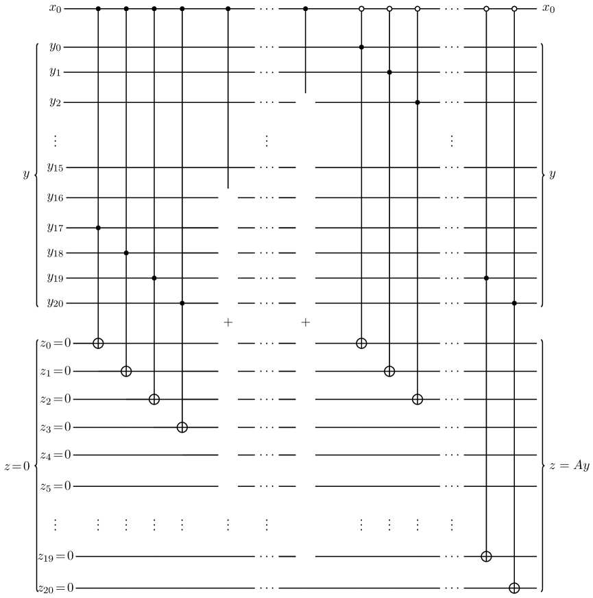
This suggests a simple and straightforward quantum algorithm for exponentiation, consisting of nothing but a sequence of controlled multiplications, as indicated in Fig. 1.
From the figure, each of the qubits, , serves as the control qubit for a separate target multiplication of by , in order to generate the next . In this basic implementation, each of the constants, , is stored by a separate bundle of qubits, initialized prior to the calculation. An additional bundle of qubits (lowest wire in Fig.1) is used to represent the value of the function. This output register is initially assigned the constant value , but through successive controlled multiplications with as described above, ends up taking on the final output value, .
For the moment, we primarily treat multiplication as an oracle or “black box” routine, whose operational details need not concern us. However, we note from the above description (and from Fig.1) that one of the two input registers gets overwritten with the product value as output, and the other is unaffected. There are indeed some multiplication algorithms—e.g. those based on the Quantum Fourier Transform (QFT) [62, 25, 3, 10, 11, 4]—that behave in this manner. We call these “overwriting” multiplication routines. Other standard multiplication algorithms—e.g., those based on bit-shifted controlled additions [12, 8, 9]—do not have this property. This issue is revisited again in Sec. IV.
As discussed, the values are stored in the -qubit output register, whereas the are stored in separate -qubit input registers. Since for all , it is convenient to represent these constants using the following -bit binary expansion:
| (8) |
Thus, the binary expansion of becomes —with the bit least significant, as discussed. This representation has a resolution of . Likewise, for all , provided (if not, there are simple remedies that can be applied, although these are not needed here). We therefore find it convenient to adopt the Eq. (8) representation for the as well as the values.
The above describes the basic algorithm for evaluating the exponential function of Eq. (1). For the Gaussian function, i.e.
| (9) |
one proceeds in exactly the same manner, except that it is necessary to perform an additional multiplication, to obtain from . We note that there are some specialized quantum squaring algorithms, that shave a bit off of the cost of a generic multiplication [8, 9, 14]. If however, this savings is not significant; the cost of the extra multiplication itself is much less than the others, since it involves only rather than qubits.

II.3 Computational cost and asymptotic scaling
In terms of memory (i.e., space) usage, the above algorithm requires qubits in all—not including the ancilla bits needed to actually implement the multiplications (not shown in Fig. 1). As mentioned, the computational cost is simply that of applying multiplications. Given the tremendous variety of multiplication algorithms that have been and will be developed—and given that some will always be better than others in different circumstances—we feel it is best to let the number of required multiplications itself serve as the appropriate gate complexity metric. Of course, this requires that multiplications comprise the overall computational bottleneck, as they do here. In similar fashion, the Toffoli count provides another implementation-independent metric—when comparing circuits whose bottleneck is the Toffoli gate (Sec. V).
If absolute costs are difficult to compare directly between different methods, then the next best thing to consider is asymptotic scaling—in this case, in terms of the parameters and . For our basic exponentiation algorithm, the scaling with respect to is clearly linear—both of the space and gate complexity.
As for the scaling with respect to , this is determined by the multiplication algorithm itself. At present, the most competitive quantum multiplication algorithm for asymptotically large in terms of scaling appears to be that of C. Gidney [14], based on the recursive Karatsuba scheme [15]. The Gidney algorithm requires space complexity, so that the overall scaling for our basic exponentiation algorithm would be . Likewise, the gate complexity for a single multiplication scales as , implying scaling for basic exponentiation.
As mentioned, Gidney does not overtake even the simplest (i.e. “schoolbook”) multiplication method until reaches a few thousand. It is therefore not practical for NISQ computing. In Sec. V, more precise estimates will be provided for absolute costs—e.g. in terms of Toffoli counts—presuming multiplication methods that can be practically applied in a NISQ context (Sec. IV). We also improve upon the basic exponentiation algorithm itself—in Sec. III, where we adopt a more efficient and refined approach, and in Sec. IV, where we present a specific, NISQ implementation.
At this point it is worthwhile to compare the two cases, and . If the exponentiation operation is itself part of a more complicated mathematical function network, with many nested inputs and outputs, then presumably one wants a generic code with sufficiently large to provide “machine precision”—i.e., or so for single precision, or for double precision. The space complexity of our basic exponentiation algorithm likely places such calculations beyond the current NISQ frontier.
On the other hand, there are situations where , and where itself may be substantially reduced. For first quantized QCC, for example, it is estimated that and may suffice to achieve the so-called “chemical accuracy” benchmark [60]. Such values place the present scheme much closer to the NISQ regime—especially once the refinements of the next section are introduced.
We conclude this subsection with a reexamination of the true cost of the Gaussian function evaluation, within the present basic scheme. Though as stated, the operation per se adds little to the direct cost, it does have the effect of squaring the size of the domain interval. Thus, if the full resolution of the domain is to be preserved, this requires rather than qubits—as well as a commensurate doubling of the gate complexity. On the other hand, this relative increase can often be largely mitigated by the improvements introduced in the subsequent sections.
III Refined Method
The basic algorithm can be substantially improved, with respect to both space and gate complexity, using the refinements described in this section. For definiteness, going forward we shall generally presume the “NISQ parameter values,” and , as discussed in Sec. II.3. However, for comparison and robustness testing, we shall occasionally use the less spartan parameter values, and (corresponding to “machine precision”). In both cases, we find that a NISQ calculation is likely feasible in the near-term future.
There are essentially two distinct ideas presented in this section to improve upon the basic algorithm—although other possible options certainly also exist. The first idea is to transform the values between successive multiplications, so that only one such constant need be stored at a time. This will have the effect of reducing the space complexity scaling to , at least for overwriting multiplications. The second idea reduces the actual number of multiplications that need be applied.
III.1 Refinement # 1: reducing space complexity
The parameters have constant values that can be determined prior to the calculation. Rather than storing them in separate registers, it is far less costly in terms of space to simply transform , prior to each successive multiplication. Such strategies have been used previously in quantum computing, when constant (unsuperposed) register values are employed [13, 8, 62]. If overwriting multiplications are used, it then becomes necessary to maintain only two such -qubit registers—i.e., one to store all of the successive values, and the other to store the (conditionally superposed) values.
The corresponding quantum circuit is presented in Fig. 2, for and . The upper of the two 21-qubit registers is used to store the , with the transformation gate used to transform into . Similarly, we define transformation gates to convert the zero state into (or vice-versa). For example, the gate is used at the start of the circuit to initialize from 0. Likewise, the lower 21-qubit register is initialized to from 0, using the transformation gate . Each successive multiplication operation (conditionally) multiplies this value by another factor of . In this manner, the total number of qubits is reduced to , or 49 for the present NISQ example—again, not including the various ancilla bits needed to effect the (overwriting) multiplications in practice.
The strategy above emphasizes minimal space complexity at the cost of greater gate depth. Alternatively, using all registers as in Sec. II, the multiplications could be performed synchronously and hierarchically, so as to minimize gate depth, but without any space reduction. In any event, our analysis in Sec. V is all based on non-overwriting multiplications (Sec. IV), for which the situation is a bit more complicated.
We next turn our attention to the implementation of the transformation gates. Since the transformations always correspond to fixed input and output values, they can easily be implemented as a set of very specific NOT gates, applied to just those qubits for which the binary expansions of Eq. (8) differ between input and output values. Hence the notation, ‘’, to refer to the resultant tensor product of NOT gates used to effect the transformation.
In Fig. 3, the specific implementation for is presented, corresponding to the specific values, , , and . The input qubits are in an unsuperposed state corresponding to the binary expansion of , as expressed in the form of Eq. (8) (with corresponding to the top wire, etc.) The output qubits are in a similar state, but corresponding to . Generally speaking, we may expect about half of the qubits to change their values. Indeed, for the present example with , we find .
In the refined algorithm as presented in Fig. 2, we find that there is one transformation required per multiplication. However, it is clear from Fig. 3 that the gate complexity of the former is trivial in comparison with that of the latter. In practical terms, therefore, the scheme of Fig. 2 can be implemented at almost no additional cost beyond that of Fig. 1—i.e., we can continue to use multiplication count as the measure of gate complexity.


III.2 Refinement # 2: reducing gate complexity
In the initial discussion that follows, it is convenient to reconsider the case. Note that for both the basic quantum algorithm of Sec. II, and the refined version of Sec. III.1, a total of multiplications are required—implying an overall gate complexity that scales asymptotically as , if Karatsuba multiplication is used. In reality, however, not all of the multiplications need be applied in practice. In fact, it will be shown in this subsection that the actual required number of multiplications, , scales as (for fixed )—thereby implying an asymptotic scaling of gate complexity no worse than .
The important realization here is that Eq. (7) implies a very rapid reduction in with increasing —essentially, as the exponential of an exponential. Consequently, there is no need to apply an explicit multiplication for any whose value is smaller than the smallest value that can be represented numerically in our fixed-point representation—i.e., , according to Eq. (8). What is needed, therefore, is an expression for in terms of and , where is the smallest such that .
For the case, it can easily be shown that
| (10) |
For the generic case where and are independent, we still never need more than multiplications. So Eq. (10) above gets replaced with the general form,
| (11) |
Clearly, scales asymptotically as either or , rather than , if is fixed. This assumes, however, that and have no implicit dependence on , which in turn depends on assumptions about how the grid points are increased. If the domain interval is expanded keeping the same spacing , or if decreases but is kept constant, then the above holds. Otherwise, as , and the prefactor becomes divergently large, implying a less favorable asymptotic scaling law.
Let us consider the case where . Since as described by Eq. (10) increases monotonically with , there is in general an interval over which , and so a reduction in the number of multiplications can be realized and . Beyond this point—i.e., for , all basic multiplications must be used. A bit of algebra reveals the following expression for the transition value:
| (12) |
As an illustrative example, consider the , , case of Sec. III.1. The formula of Eq. (10) predicts that multiplications will be required, exactly as indicated in Fig. 2. This represents a significant reduction versus the multiplications that would otherwise be needed. As confirmation that is correct, we note that , which is larger than . However, .
Finally, we can compute from Eq. (12)—which, with the above and values, is found to be . Thus, one finds a reduction in down from , over about 80% of the range of possible values. Now consider the Gaussian rather than exponential function, for which . Here, we find —implying that there is almost always a reduction in . We will discuss further ramifications in Secs. IV and V.
III.3 Second half of refined quantum algorithm
Although the second refinement of Sec. III.2, can lead to fewer than multiplications (depending on the values of , , and ), this does not imply that the refined quantum algorithm simply ends at the right edge of Fig. 2. There remains a subsequent computation that must occur, using the qubits, in order to ensure that the correct final value for the function is obtained. The multiplication count of the additional computation is zero, although it does add a cost of Fredkin gates.
Consider that when is a power of two, then all but the binary expansion coefficients in Eq. (5) vanish, and the function value becomes simply , according to Eq. (6). This implies that for any , is smaller than the minimum non-zero number that can be represented, and so should be replaced with . This situation will occur if any of the qubits, , are in their 1 states. Otherwise—i.e., if all of the are in their 0 states so that —then nothing should happen, as the lowest register is already set to the correct output value, , at the right edge of Fig. 2.
The above can be implemented as follows. First, for the case , no additional circuitry is needed; one simply runs the quantum circuit of Fig. 2 as is, except with explicit controlled multiplications across all of the qubits. For the case , then controlled mutiplications are implemented across the lowest qubits, . The final qubit, is then used to conditionally set the lowest register to zero.
For the last case where , we apply the quantum circuit indicated in Fig. 4. This requires first checking if any of the qubits are in state 1, which is implemented using a sequence of OR gates. The first is applied to and to compute . If needed, that output is then sent to a second OR gate along with , etc. The final output, which will serve as a control qubit, has value 1 if any of the are in their 1 states; otherwise, it has value 0.
Meanwhile, the upper of the two -qubit registers, which starts out representing the constant value , is transformed to the value 0, using the transformation gate, . Finally, the upper and lower -qubit registers undergo a controlled , applied in qubit-wise or tensor-product fashion, across all qubits of the two registers. If the swap occurs, then the function output as represented by the lower of the two -qubit registers becomes zero; otherwise, it is left alone.
We conclude this subsection with a discussion of the reversible quantum OR gate, used in the quantum circuit of Fig. 4. Such a gate can be easily constructed from a single reversible NAND (Toffoli) gate, together with various NOT gates, as indicated in Fig. 5. Note that each such OR gate introduces one new ancilla qubit, initialized to the 1 state. There are thus no more than additional ancilla qubits in all that get introduced in this fashion. The additional costs associated with Fig. 4, in terms of both gates and qubits, are thus both very small as compared to those of Fig. 2, although they will be included in resource calculations going forward.

IV Detailed Implementation Suitable for NISQ Computing
IV.1 Overview
As discussed, there is large variety of quantum multiplication algorithms on the market currently [10, 11, 4, 12, 8, 9, 13, 14, 15, 16], and no doubt many more will follow. In part for this reason, we prefer to rely on the “multiplication count” metric for gate complexity. Indeed, whereas current multiplication algorithms largely make use of integer or fixed-point arithmetic, floating-point algorithms—which have very different implementations—are also of interest going forward, especially for exponentiation. The multiplication count metric will continue to be relevant for all such innovations.
On the other hand, we are also interested in developing a specific exponentiation circuit that can be run on NISQ computers for realistic applications. Moreover, we aim to compare performance against the state-of-the-art competing method by Häner and coworkers [8], for which multiplications are not the only bottleneck. This constrains us in two important ways. First, we cannot use the multiplication count metric for accurate comparison; instead, since the Häner algorithm is Toffoli-based (as is our circuit), we use the Toffoli count metric. Second, to the extent that both exponentiation algorithms do rely on multiplications, similar multiplication subroutines should be used for both.
Accordingly, we use a modified version of Häner’s multiplication subroutine, which is itself a fixed-point version of “schoolbook” integer multiplication [12, 8, 9, 13, 14], based on bit shifts and controlled additions. In particular, they exploit truncated additions (that maintain fixed bits of precision), together with a highly efficient overwriting, controlled, ripple-carry addition circuit by Takahashi [17, 18, 19, 13] that minimizes both space and gate complexities. As it happens, there are some further improvements and simplifications that arise naturally for our particular exponentiation context, which we also exploit. All of this is described in detail in Secs. IV.2 and V, wherein we also derive fairly accurate resource estimates for both qubit and Toffoli counts, respectively.
One disadvantage of Häner multiplication is that it does not overwrite the multiplier input—the way, e.g., that QFT multiplication would [10, 11, 4]. Consequently, each successive multiplication requires additional ancilla bits, unlike what is presumed in Fig. 2. Space needs are accordingly greater in this implementation than what is described in Sec. III.1—becoming essentially qubits rather than (without ancilla). For the NISQ applications of interest here, is still quite small, and so the increase is generally not too onerous. It is more of a concern for the Gaussian evaluations, for which can in principle get twice as large as the corresponding exponential value.
Of course, it would be possible to employ QFT-based multiplication in our exponentiation algorithm—which would require qubits, with ancilla included. On the other hand, the QFT approach is not Toffoli-based, and would therefore not lend itself to direct comparison with Häner, vis-à-vis gate complexity. In order to estimate a Toffoli count for QFT multiplication, one would have to presume some specific implementation for the Toffoli gate itself (e.g., in terms of T gates), which is not ideal [13]. In any event, Toffoli counts have become a standard gate complexity metric in quantum computing.
For these reasons, overwriting QFT-based multiplications are not considered further here. Instead, for cases where the increased space complexity of the non-overwriting multipliers might pose a problem, we address this situation through the use of a simple alternative algorithm, describe in Sec. IV.3, that trades increased gate complexity for reduced space complexity—essentially by uncomputing intermediate results. In principle, there are any number of “reversible pebbling strategies” [13, 8, 14, 63] that might also be applied towards this purpose. The particular approach adopted here, though, is very simple, and appears to be quite effective.
IV.2 Non-overwriting controlled quantum mutiplication
As discussed, non-overwriting controlled-addition multiplication subroutines have three registers. The first is an input register for the multiplier; the second is another input register for the multiplicand; the third is the output or “accumulator” register. The accumulator register is initialized to zero, and therefore serves as an ancilla register, but comes to store the product of the multiplier and multiplicand at the end of the calculation.
For integer multiplication, the accumulator register requires qubits, assuming that both input registers are qubits each. The first register (multiplier) provides the the control qubits for a cascade of controlled additions. The second register (multiplicand) serves as the first input for each controlled addition. The second input for each controlled addition is a successively bit-shifted subset of qubits from the accumulator register. Note that overwriting controlled additions are used, so that for each controlled addition, the second register output is the sum of the two inputs.
In the case of our exponentiation algorithm, we propose a version of the above basic scheme that is modified in two very important ways. First, the ’th multiplication is controlled, via the domain qubit (Fig. 2). Second, the circuit exploits the fact that every multiplier has a fixed (unsuperposed) value—i.e. the constant, . Adding an overall control to a quantum circuit tends to complicate that circuit—turning CNOT gates into CCNOT gates, etc. On the other hand, the fixed multiplier enables substantial simplifications—of the type used in Shor’s algorithm for factoring integers [13, 62], for instance.
Specifically, we no longer treat the multiplier as an input register—for there is no longer a need to use the qubits as control bits for the additions. Instead, the binary expansion of from Eq. (8) is used to hard-wire what would be a set of uncontrolled additions, directly into the quantum circuit—but only for those binary expansion coefficients equal to 1. In addition to reducing the set of inputs by one entire -bit register, this modification also reduces the number of additions that must be performed by a factor of two—since on average, only half of the expansion coefficients have the value 1.
In addition to the above advantages, fixed-multiplier multiplication reduces circuit complexity by replacing controlled with uncontrolled additions—effectively converting CCNOT gates to CNOT gates. Of course, when the qubit control is thrown back in, to create the requisite controlled multiplication subroutine, we find that the additions become controlled after all—but by , rather than . In effect, the control bit for the multiplication is simply passed down to the individual controlled additions which comprise it.
The above can all be seen in Fig. 6, our detailed quantum circuit for controlled multiplication, as implemented for the first multiplication in Fig. 2, denoted ‘’ (i.e., multiplication by , controlled by the qubit). Note that the individual multiplication circuits, , differ from each other, due to the different binary expansions. Once again, our canonical NISQ parameter values are presumed, i.e., , , and .
From the figure, another important difference from the basic scheme may be observed: the accumulator register, , has only rather than qubits. This is because fixed-point rather than integer arithmetic is being used—as a consequence of which, it is not necessary to store what would otherwise be the least significant bits of the product. This situation provides yet another benefit, which is that each controlled addition becomes “truncated” to an -bit operation—with increasing with each successive controlled addition across the range, .
Note that the smallest possible addition corresponds to rather than . This is because the first controlled addition can be replaced with a cascade of Toffoli gates—or controlled bit-copy operations—which is a much more efficient implementation. This substitution works because the accumulator register is set to zero initially. The very first controlled addition thus always (conditionally) adds the multiplicand register to zero.
For the example in the figure, the first four binary expansion coefficients for (from right to left) are all zero; these bits are simply ignored. The first coefficient equal to one is the or fifth bit. As indicated in Fig. 6, this causes the last four bits of the multiplicand register to be (conditionally) copied into the first four bits of the accumulator register—in what would otherwise be an controlled addition. The bit is also equal to one, leading to the first bona fide controlled addition in Fig. 6, with . This pattern continues until the the next-to-last, or bit is reached, which is the last bit equal to one. This leads to the final controlled addition, with .
Although the last () bit is zero, even if it were equal to one, the corresponding controlled addition gate would extend only up to . Thus, the top wire, , or least-significant bit of the multiplicand, is never used. This reflects the fact that both numbers being multiplied have values less than one, and that fixed bits of precision are maintained throughout the calculation. Note also that, as a result, there are never any overflow errors.
The final part of the controlled multiplication circuit is a cascade of controlled bit-copy operations (i.e., modified Toffoli gates), which conditionally set the final output of the accumulator register equal to , when (hence the open circles). Otherwise, this register would remain zero. Thus, the “do nothing” instruction in Sec. II.2 does not literally mean “do nothing” when non-overwriting multiplications are used, as it is still necessary to copy the multiplicand input register to the accumulator output register.
IV.3 Quantum algorithm for exponentiation: space saving alternative
Now that the specific, controlled quantum multiplication algorithm of Sec. IV.2 has been identified, we can determine a precise estimate of space requirements for our overall exponentiation circuit. (Gate complexity will be discussed in Sec. V.1). As noted, each of the multiplications requires a clean -qubit ancilla bundle as input for its accumulator register, together with the (accumulator) output from the most recent multiplication as input for its multiplicand register. Thus, for successive multiplications, separate registers would be required in all.
However, we can realize significant savings—i.e., one entire register of space, and one entire controlled multiplication subroutine—by exploiting the fact that the first multiplicand (i.e., ) is a fixed constant. The first controlled multiplication, , is therefore a controlled multiplication of the constant by the constant . Since both constants are fixed, the controlled multiplication can be much more efficiently realized using two controlled transformation gates acting on a single register (i.e., the first two gates shown in Fig. 7) rather than the controlled multiplication circuit of Fig. 6. Note that this controlled implementation uses only CNOT gates; thus the Toffoli count is zero.
Since Takahashi addition does not use additional ancilla qubits [18, 19], the total number of qubits required to implement the multiplications is just . In addition to this, we have the qubits needed to store the domain register, , that is used to supply the control qubits. The current qubit count is thus .
However, if , then the second half of the refined exponentiation circuit (i.e., Fig. 4) must also be executed, which introduces some additional space overhead. To begin with, our current reliance on non-overwriting multiplications implies that we can no longer generate the requisite zero ancilla register (i.e., the next-to-last register in the figure) without significant (un)computation. To avoid this, we instead add a clean new register—at the additional cost of new qubits. In addition to this, there are the ancilla bits used by the OR gates, as discussed in Sec. III.3). Altogether then, the total qubit count becomes:
| (13) |
To reduce qubit counts in cases where Eq. (13) renders a NISQ calculation unfeasible, we have developed a “space-saving” alternative algorithm. The general idea is to uncompute some of the intermediate quantities, in order to restore some of the ancilla registers to their initial clean state, so that they can then be reused for subsequent computations. Of course, this requires additional overhead—i.e., in our case, additional controlled multiplications.
More specifically, our space-saving algorithm reduces space requirements from down to —a very marked reduction, especially if is reasonably large. The added cost in terms of gate complexity, on the other hand, is never more than double that of our original algorithm described above. Thus, , with the multiplication count for the space-saving approach.
For values of that lie in the range
| (14) |
(where is an integer), the space-saving method requires a total of -qubit registers to perform all multiplications. Note that the restriction implies that the method is only applicable for . However, the case presents minimal space requirements, and so the space-saving approach is less likely to be needed. In any event, for all numerical examples considered in Sec. V.2, (including the worst Gaussian cases), .
The total qubit count for the space-saving alternative algorithm can be shown to be as follows:
| (15) |
Note that unlike our original non-space-saving or “gate-saving” algorithm, a zero -qubit ancilla register can always be made available for the final controlled operation of Fig. 4—except when , which thus has an additional qubit cost. (See technical note at the end of this subsection).
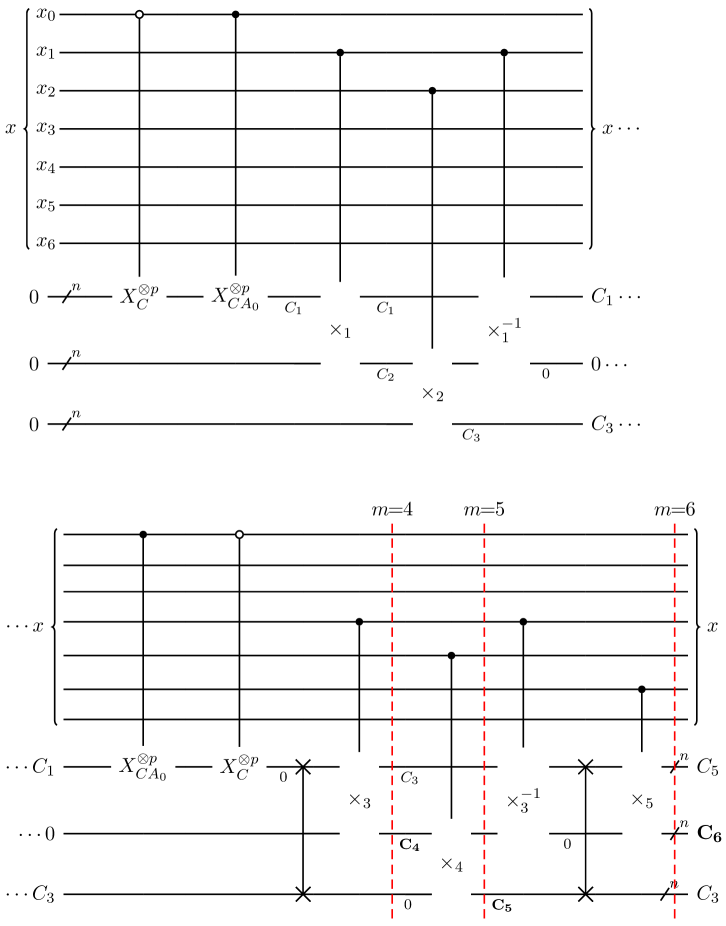
The space-saving algorithm itself proceeds as follows. First, apply the first multiplications, exactly as for the earlier gate-saving algorithm. This leaves the registers in the states, , , …, . Then, uncompute all but the most recent multiplication (i.e., the one that provided ). The first registers are thereby restored to zero, but the final register remains in the state. It is then possible to perform additional multiplications, before once again running out of registers. All but the last of these is then uncomputed, allowing more multiplications to be performed, and so on.
The space-saving quantum circuit used for and 4–6 is presented in Fig. 7, corresponding to registers. For the first wave, there are three clean registers, allowing for three successive multiplications, , , and (provided is implemented as discussed above). This is followed by two uncompute multiplications for the first two multiplications, denoted and (the latter, again with the new implementation). In the second wave, we apply and , generating and , respectively. This suffices for and , respectively. However, if , we must undergo a third and final wave, as indicated in the figure.
As is clear from the above description, and from Fig. 7, the number of uncompute multiplications, , is always less than . Thus, , as claimed. Precise values can be found as follows. Let be the largest integer such that
| (16) |
Then,
| (17) |
Table 1 indicates specific values for all . Note that the multiplication count includes both and ; thus, the total actual number of controlled multiplication subroutines that must be executed is , as indicated in the final column. From the table, also, it may be observed that greater space savings are usually associated with increased multiplication counts, and vice-versa.
Technical note: For space-saving calculations, a zero ancilla register is automatically available at the end of the Fig. 7 circuit (to be used in the subsequent Fig. 4 circuit), whenever Eq. (16) is a true inequality. When Eq. (16) is an equality, then the case requires the addition of a new zero ancilla register (as discussed), but for , a zero register can be easily created from an existing non-zero register. This is done by applying the single uncompute multiplication, . As an example, the case corresponds to and , thus satisfying Eq. (16) as an equality, with both sides equal to one. The necessary uncompute multiplication can be seen in Fig. 7, just to the right of the vertical dashed line marked ‘’. Note that the Toffoli count associated with such multiplications is greatly reduced in comparison with the other multiplications, as will be discussed in Sec. V.1. Moreover, this event is fairly rarely realized in practice, including the examples given in the present work. Nevertheless, the small additional cost required in such cases is included in the Toffoli count formulas presented in Sec. V.1.
| 4 | 3 | 2 | 4 |
| 5 | 3 | 2 | 5 |
| 6 | 3 | 3 | 7 |
| 7 | 4 | 3 | 8 |
| 8 | 4 | 5 | 11 |
| 9 | 4 | 5 | 12 |
| 10 | 4 | 6 | 14 |
| 11 | 5 | 7 | 16 |
| 12 | 5 | 7 | 17 |
| 13 | 5 | 9 | 20 |
| 14 | 5 | 9 | 21 |
| 15 | 5 | 10 | 23 |
| 16 | 6 | 12 | 26 |
| 17 | 6 | 12 | 27 |
| 18 | 6 | 12 | 28 |
| 19 | 6 | 14 | 31 |
| 20 | 6 | 14 | 32 |
| 21 | 6 | 15 | 34 |
| 22 | 7 | 15 | 35 |
| 23 | 7 | 18 | 39 |
| 24 | 7 | 18 | 40 |
| 25 | 7 | 18 | 41 |
| 26 | 7 | 20 | 44 |
| 27 | 7 | 20 | 45 |
| 28 | 7 | 21 | 47 |
| 29 | 8 | 22 | 49 |
| 30 | 8 | 22 | 50 |
| 31 | 8 | 25 | 54 |
| 32 | 8 | 25 | 55 |
| 33 | 8 | 25 | 56 |
| 34 | 8 | 27 | 59 |
| 35 | 8 | 27 | 60 |
| 36 | 8 | 28 | 62 |
V Analysis: Toffoli counts
V.1 Present methods
To a rough approximation, the total Toffoli count for the proposed exponentiation algorithm [or for the space-saving alternative] is simply [or ] times the Toffoli count needed to execute a single controlled multiplication subroutine. Before working out the latter, however, we first describe another reduction of effort that in practical terms, converts the total cost to that of only [or ] controlled multiplications. This additional savings is fully realized whenever , which in practice occurs much of the time, if the domain interval is realistically large.
The rationale is as follows. When , the values span the entire range from 1 down to . This implies that for , the corresponding have many leading zeroes. Consequently, these later multiplications can be performed using fewer than binary digits, leading to significant computational savings.
Note that the worst-case scenario vis-à-vis the aforementioned savings—i.e., that for which the have the fewest leading zeros—corresponds to from below. Now, in general, the approximate number of leading zeros for the binary expansion of is given by . Thus, for , we find leading zeros, as expected. More generally, Eq. (7) in the worst-case scenario leads to
| (18) |
where . The number of binary digits needed for the controlled multiplication is thus .
Going forward, we shall for simplicity presume the asymptotic limit, . In this limit, the Toffoli count per multiplication scales as . The Toffoli savings (i.e., reduction in the Toffoli count relative to multiplication with digits) is therefore
| (19) |
Summing Eq. (19) from to then yields a total savings of multiplications.
In practice—i.e., for finite —the series is truncated, and so the actual savings is less than multiplications. In the worst case (of the worst case), only the term contributes to the sum, resulting in a lower bound of multiplications. On the other hand, a small increase in , such that the new value is slightly greater than , will increment the value of —thus, effectively increasing the savings by one whole additional multiplication. On balance, we therefore take our “best case of the worst case” value as a reasonable middle-ground estimate.
Next, we move on to a calculation of the Toffoli cost of each controlled multiplication. As discussed in Sec. IV.2, these are implemented using a sequence of controlled additions, with from qubits up to qubits. Note that the Toffoli cost of the highly efficient overwriting, controlled, ripple-carry addition circuit of Takahashi [18, 19, 8] with qubits is . Thus, if every required a controlled addition, the total contribution to the Toffoli cost of multiplication would be . However, since only half of these multiplications are realized on average, in practice, the actual cost per multiplication is half of this. The total contribution to the cost of the exponentiation circuit is then this value, multiplied by the effective number of multiplications, i.e. .
Now, in addition, each controlled multiplication in the Fig. 6 circuit also begins and ends with a cascade of additional Toffoli gates. The initial cascade can be easily shown to consist of two Toffoli gates, on average. The final cascade, is always Toffoli gates, even when fewer than qubits are needed to execute the main part of the multiplication circuit (i.e., the controlled additions). Note that both Toffoli cascades are required in every actual multiplication. The total contribution to the Toffoli cost of the exponentiation circuit is thus .
Finally, there are the additional costs associated with the second half of the (refined) exponentiation circuit, as presented in Fig. 4, presuming . Since each Fredkin gate can be implemented using a single Toffoli gate, the Toffoli cost of the final operation is . Likewise, each OR gate requires one Toffoli gate, for a total Toffoli count of . Altogether, we wind up with the following expression for the total Toffoli cost for the entire gate-saving exponentiation circuit:
| (20) |
Things are a bit more complicated in the space-saving algorithm case. In particular, there are three cases instead of two. In addition to , there are two different cases, i.e. one corresponding Eq. (16) being an equality, and one to the inequality case, as discussed in the Technical note at the end of Sec. IV.3. Note also that the uncompute multiplications that are not included in (as compared to ) are in fact the multiplications, that do not cost as much. Consequently, the effective number of uncompute multiplications is reduced relative to the actual number, by an amount less than 5/3 multiplications. A more accurate estimate of the uncompute savings is given by
| (21) |
where .
Taking all of the above into account, we obtain the following expression for the Toffoli count of the space-saving exponentiation algorithm:
| (22) |
Note that in the final case above, the (worst-case) cost of the additional uncompute multiplication is obtained from in Eq. (19) to be that of a regular multiplication—at least insofar as the controlled addition contribution is concerned.
V.2 Explicit numerical comparison with Häner approach
In the approach by Häner et al. [8], arbitrary functions are evaluated via a decomposition of the domain into non-intersecting subdomain intervals, as discussed in Sec. I. A given function is then approximated using a separate ’th order polynomial in each subdomain. Both the polynomial coefficients, and the subdomain intervals themselves, are optimized for a given target accuracy, using the Remez algorithm [64].
Once the optimized parameters have been determined for a given function , domain interval , and (Häner) value, the quantum algorithm is then implemented as follows. First, polynomials are evaluated using a sequence of multiplication-accumulation (addition) operations. On a quantum platform, these can be performed in parallel, across all subdomains at once, using conditioned determination of the coefficients for each subdomain. The multiplication count would thus be , irrespective of . Also, since non-overwriting multiplications are used, the qubit count is .
Note that generally speaking, lower corresponds to greater , and vice-versa. Thus, were the above multiplication-accumulation operations the only significant computational cost, one would simply choose a very small value such as . However, there is additional space and gate complexity overhead associated with managing and assigning the sets of polynomial coefficients. These costs do increase with (although in a manner that is naturally measured in Toffoli gates rather than multiplications). There is thus a competition between and , with minimal Toffoli counts resulting when or 5—at least for the numerical examples from Ref. 8 that are considered here.
The minimal-Toffoli choice of can thus be thought of as a “gate-saving” Häner implementation. Note that a rudimentary “space-saving” alternative may also be obtained, simply by reducing the value of . That said, Ref. 8 also discusses the use of much more sophisticated pebbling strategies. However, such strategies are not actually implemented for the numerical results presented in Ref. 8 that are used for comparison with the present results.
Instead, Häner and coworkers perform calculations for different functions, and for different target accuracies, across a range of different values—providing total qubit and Toffoli counts for each. In particular, they consider both the exponential and Gaussian functions, with and . It thus becomes mostly possible to provide a direct comparison between the Häner approach and our methods, with respect to these metrics. Such a comparison is provided in Table 2.
One slight difficulty arises from the fact that no value is provided in Ref. 8; moreover, the authors have not been available for clarification. We thus present results for our methods using two very different values—i.e., 10 and 100. Although for most purposes, even the former interval is wide enough to capture the main function features, the latter interval is actually more realistic for certain applications such as QCC (as discussed in greater detail in Sec. VI). In any case, it should be mentioned that in the large limit, our methods become less expensive, whereas the Häner approach becomes more expensive—owing to the increased values needed to achieve a given level of accuracy.
The issue of target range accuracy merits further discussion. In Häner, calculations were performed to an accuracy of , and also . The corresponding number of bits needed to resolve the range to these thresholds are 23.25 and 29.89, respectively. Note that these values are quite close to the and values considered in our examples thus far—in one case a bit high, in the other a bit low. Of course, a few extra bits might also be needed to compensate for round-off error in the fixed-point arithmetic. These are relatively small effects however; in particular, they are likely no larger than those associated with the unknown Häner value.
For our purposes, therefore, we take these values as reasonable estimates, at least for the exponential function evaluations. For the Gaussian case, we do go ahead and use and , as the closest integers larger than the threshold values listed above. As for the corresponding values, roughly speaking, these would be double those from the exponential calculation—except that we exploit symmetry of the domain to reduce these by one bit each. Thus, and , respectively, for and .
In Table 2, we present Toffoli and qubit counts for both function evaluations (i.e., exponential and Gaussian), for both target accuracy thresholds (i.e. and ), for both of our methods (i.e. gate-saving and space-saving), and for both domain intervals (i.e. and ). For each function, the minimal Toffoli count is given in bold face. For each function and accuracy threshold, we also present results for the full set of Häner calculations, as obtained from Ref. 8. Here too, the minimal Toffoli count is highlighted in bold face.
In all cases, our method requires far fewer Toffoli gates than the Häner approach. In comparing minimal-Toffoli calculations for the exponential function, the Toffoli count is reduced from 15,690 using Häner, down to just 912 using our approach. For Gaussian function evaluation, the Toffoli count comparison is even more stark—i.e., 19,090 vs. just 704. Generally speaking, our methods also require fewer qubits than Häner. This is especially true for the space-saving alternative, which in one instance requires as few as 71 qubits (and 1409 Toffoli gates)—a NISQ calculation, certainly, by any standard.
| Function | Method | Domain | Accuracy | Accuracy | ||||
|---|---|---|---|---|---|---|---|---|
| interval | Toffolis | qubits | Toffolis | qubits | ||||
| gate saving | 1620 | 154 | 4438 | 264 | ||||
| 912 | 134 | 2828 | 233 | |||||
| space saving | 2308 | 91 | 7531 | 136 | ||||
| 1409 | 71 | 4278 | 105 | |||||
| Häner | 17304 | 149 | 45012 | 175 | ||||
| 15690 | 184 | 28302 | 216 | |||||
| 16956 | 220 | 25721 | 257 | |||||
| 18662 | 255 | 26452 | 298 | |||||
| gate saving | 4468 | 325 | 8300 | 465 | ||||
| 704 | 141 | 3232 | 262 | |||||
| space saving | 7546 | 133 | 14479 | 165 | ||||
| 962 | 93 | 5018 | 142 | |||||
| Häner | 20504 | 161 | 49032 | 187 | ||||
| 19090 | 199 | 32305 | 231 | |||||
| 21180 | 238 | 30234 | 275 | |||||
| 23254 | 276 | 31595 | 319 | |||||
VI Summary and Conclusions
After the various refinements and NISQ-oriented details as presented in the latter 2/3 of this paper, it might be easy to lose sight of the main point, which is simply this: the method presented here allows the exponential function to be evaluated on quantum computers for the cost of a few multiplications. This basic conclusion will continue to hold true, regardless of the many quantum hardware and software innovations that will come on the scene in ensuing decades.
In particular, there is a plethora of multiplication algorithms available, both overwriting (e.g. QFT-based) and non-overwriting (e.g. controlled addition), and for both integer and fixed-point arithmetic—with new strategies for floating-point arithmetic, quantum error correction, etc., an area of ongoing development. Given this milieu, we propose the implementation-independent “multiplication count” as the most sensible gate complexity metric, for any quantum algorithm whose dominant cost can be expressed in terms of multiplications. The present algorithms are certainly of this type.
For our exponentiation strategy, the (controlled) multiplication count will indeed be rather small in practice—at least for the applications envisioned. To begin with, in a great many simulation contexts, the domain resolution as expressed in total qubits , is far less than the range resolution —with . For QCC, for instance, the and values considered throughout this work are likely to suffice in practice [60]. Conversely, we also consider the asymptotically large limit, in which it can be shown [in Eq. (10)] that for fixed . In this limit, Karatsuba multiplication provides better asymptotic scaling. Using the Gidney implementation, the Toffoli and qubit counts for exponentiation scale as and , respectively.
In the latter part of this paper, we present two specific, NISQ implementations of our general exponentiation strategy, in order that detailed resource estimates can be assessed, and compared with competing methods. When compared with the method of Häner and coworkers, our implementations are found to reduce Toffoli counts by an order of magnitude or more. Qubit counts are also (generally) substantially reduced. Note that our two implementations are complementary, with one designed to favor gate and the other space resource needs. Together, they may provide the flexibility needed to actually implement exponentiation on NISQ architectures—which could serve as the focus of a future project.
Finally, we assess the present exponentiation algorithms within the context in which they were originally conceived—i.e., quantum computational chemistry (QCC). The long-awaited “(QCC) revolution”[21, 22, 23, 1, 2, 24, 25, 3, 26, 27, 28, 29, 30, 31, 5, 32, 33, 34, 35, 36, 37, 38, 39, 40, 41, 42, 43, 44, 7, 45, 46]” may be nearly upon us, although achieving full quantum supremacy will likely require quantum platforms that can accommodate first-quantized methods. On classical computers, the Cartesian-component separated (CCS) approach, as developed by the author [57, 58, 59, 60, 61] offers a highly competitive first-quantized strategy.
On quantum computers, the question appears to boil down to the relative costs of the exponential function vs. the inverse square root [65]. Toffoli count estimates for the former appear in Table 2. Note that the larger-domain-interval calculations—i.e., those with lower Toffoli counts—are the more realistic in this context. This is because the QCC CCS implementation requires multiple exponentiations with different values to be performed, across the same grid domain interval—which must accordingly be large enough to accommodate all of them. Our exponentiation cost of 704 Toffoli gates should thus be compared to the cost of the inverse-square-root function, which—again, according to the highly optimized method of Häner and coworkers—is estimated to be 134,302 Toffoli gates.
Acknowledgement
The author gratefully acknowledges support from a grant from the Robert A. Welch Foundation (D-1523).
References
- Abrams and Lloyd [1997] D. S. Abrams and S. Lloyd, Phys. Rev. Lett., 1997, 79, 2586–2589.
- Zalka [1998] C. Zalka, Proc. Royal Soc. London A, 1998, 454, 313.
- Nielsen and Chuang [2000] M. A. Nielsen and I. L. Chuang, Quantum Computation and Quantum Information, Cambridge Univ Press, 2000.
- Florio and Picca [2004] G. Florio and D. Picca, arXiv preprint arXiv:2004.0407079 [quant-ph], 2004.
- Kais et al. [2014] S. Kais, S. A. Rice and A. R. Dinner, Quantum information and computation for chemistry, John Wiley & Sons, 2014.
- Preskill [2018] J. Preskill, arXiv preprint arXiv:1801.00862v3 [quant-ph], 2018.
- Alexeev et al. [2019] Y. Alexeev, D. Bacon, K. R. Brown, R. Calderbank, L. D. Carr, F. T. Chong, B. DeMarco, D. Englund, E. Farhi and B. Fefferman, et al., arXiv preprint arXiv:1912.07577, 2019.
- Häner et al. [2018] T. Häner, M. Roetteler and K. M. Svore, arXiv preprint arXiv:1805.12445v1 [quant-ph], 2018.
- Sanders et al. [2020] Y. R. Sanders, D. W. Berry, P. C. Costa, L. W. Tessler, N. Wiebe, C. Gidney, H. Neven and R. Babbush, Phys. Rev. X Quantum, 2020, 1, 020312.
- Draper [2000] T. G. Draper, arXiv preprint arXiv:quant-ph/0008033v1, 2000.
- Florio and Picca [2004] G. Florio and D. Picca, arXiv preprint arXiv:2004.0403048 [quant-ph], 2004.
- Häner et al. [2017] T. Häner, M. Roetteler and K. M. Svore, Quantum Information and Computation, 2017, 18, 673–684.
- Parent et al. [2017] A. Parent, M. Roetteler and M. Mosca, 12th Conference on the Theory of Quantum Computation, Communication, and Cryptography (TQC 2017), Germany, 2017, pp. 7:1–7:15.
- Gidney [2019] C. Gidney, arXiv preprint arXiv:1904.07356v1 [quant-ph], 2019.
- Karatsuba and Ofman [1962] A. Karatsuba and Y. Ofman, Doklady Akad. Nauk SSSR, 1962, 145, 293–294.
- Kowada et al. [2006] L. A. B. Kowada, R. Portugal and C. M. H. de Figueiredo, Journal of Universal Computer Science, 2006, 12, 499–511.
- Cuccaro et al. [2004] S. A. Cuccaro, T. G. Draper, S. A. Kutin and D. P. Moulton, arXiv preprint arXiv:quant-ph/0410184, 2004.
- Takahashi [2008] Y. Takahashi, Ph.D. thesis, The University of Electro-Communications, 2008.
- Takahashi et al. [2009] Y. Takahashi, S. Tani and N. Kunihiro, arXiv preprint arXiv:0910.2530v1 [quant-ph], 2009.
- Bharti et al. [2021] K. Bharti, A. Cervera-Lierta, T. H. Kyaw, T. Huag, S. Alperin-Lea, A. Anand, M. Degroote, H. Heimonen, J. S. Kottmann, T. Menke, W.-K. Mok, S. Sim, L.-C. Kwek and A. Aspuru-Guzik, arXiv preprint arXiv:2101:08448v1 [quant-ph], 2021.
- Poplavskii [1975] R. P. Poplavskii, Usp. Fiz. Nauk., 1975, 115, 465–501.
- Feynman [1982] R. P. Feynman, Int. J. Theor. Phys, 1982, 21, 467–488.
- Lloyd [1996] S. Lloyd, Science, 1996, 273, 1073–1078.
- Lidar and Wang [1999] D. A. Lidar and H. A. Wang, Phys. Rev. E, 1999, 59, 2429.
- Abrams and Lloyd [1999] D. S. Abrams and S. Lloyd, Phys. Rev. Lett., 1999, 83, 5162.
- Aspuru-Guzik et al. [2005] A. Aspuru-Guzik, A. D. Dutoi, P. J. Love and M. Head-Gordon, Science, 2005, 309, 1704.
- Kassal et al. [2008] I. Kassal, S. P. Jordan, P. J. Love, M. Mohseni and A. Aspuru-Guzik, Proc. Nat’l Acad. Sci, 2008, 105, 18681.
- Whitfield et al. [2010] J. D. Whitfield, J. Biamonte and A. Aspuru-Guzik, arXiv preprint arXiv:1001.3885 [quant-ph], 2010.
- Brown et al. [2010] K. L. Brown, W. J. Munro and V. M. Kendon, Entropy, 2010, 12, 2268–2307.
- Christiansen [2012] O. Christiansen, Phys. Chem. Chem. Phys., 2012, 14, 6672.
- Georgescu et al. [2014] I. M. Georgescu, S. Ashhab and F. Nori, Rev. Mod. Phys., 2014, 86, 153.
- Huh et al. [2015] J. Huh, G. G. Guerreschi, B. Peropadre, J. R. McClean and A. Aspuru-Guzik, Nature Photonics, 2015, 9, 615.
- Babbush [2015] R. Babbush, Ph.D. thesis, Harvard University, 2015.
- Kivlichan et al. [2017] I. D. Kivlichan, N. Wiebe, R. Babbush and A. Aspuru-Guzik, J. Phys. A: Math Theo, 2017, 50, 305301.
- Babbush et al. [2018] R. Babbush, D. W. Berry, Y. R. Sanders, I. D. Kivlichan, A. Scherer, A. Y. Wei, P. J. Love and A. Aspuru-Guzik, Quantum Sci. Technol., 2018, 3, 015006.
- Babbush et al. [2018] R. Babbush, N. Wiebe, J. McClean, J. McClain, H. Neven and G. K.-L. Chan, Phys. Rev. X, 2018, 8, 011044.
- Babbush et al. [2018] R. Babbush, C. Gidney, D. W. Berry, N. Wiebe, J. McClean, A. Paler, A. Fowler and H. Neven, Phys. Rev. X, 2018, 8, 041015.
- Babbush et al. [2019] R. Babbush, D. W. Berry, J. R. McClean and H. Neven, npj Quantum Information, 2019, 5, 92.
- Low et al. [2019] G. H. Low, N. P. Bauman, C. E. Granade, B. Peng, N. Wiebe, E. J. Bylaska, D. Wecker, S. Krishnamoorthy, M. Roetteler, K. Kowalski, M. Troyer and N. A. Baker, arXiv preprint arXiv:1904.01131v1 [quant-ph], 2019.
- Kivlichan et al. [2019] I. D. Kivlichan, C. Gidney, D. W. Berry, N. Wiebe, J. McClean, W. Sun, Z. Jiang, N. Rubin, A. Fowler, A. Aspuru-Guzik, R. Babbush and H. Neven, arXiv preprint arXiv:1902.10673, 2019.
- Izmaylov et al. [2019] A. Izmaylov, T.-C. Yen and llya G. Ryabinkin, Chemical Science, 2019, 10, 3746.
- Parrish et al. [2019] R. M. Parrish, E. G. Hohenstein, P. L. McMahon and T. J. Martinez, arXiv preprint arXiv:1901.01234v1 [quant-ph], 2019.
- Altman et al. [2019] E. Altman, K. R. Brown, G. Carleo, L. D. Carr, E. Demler, C. Chin, B. DeMarco, S. E. Economou, M. Eriksson and K.-M. Fu, arXiv preprint arXiv:1912.06938, 2019.
- Cao et al. [2019] Y. Cao, J. Romero, J. P. Olson, M. Degroote, P. D. Johnson, M. Kieferova, I. D. Kivlichan, T. Menke, B. Peropadre, N. P. D. Sawaya, S. Sim, L. Veis and A. Aspuru-Guzik, Chem. Reviews, 2019, 119, 10856.
- Bauer et al. [2020] B. Bauer, S. Bravyi, M. Motta and G. K. Chan, arXiv preprint arXiv:2001.03685, 2020.
- McArdle et al. [2020] S. McArdle, S. Endo, A. Aspuru-Guzik, S. Benjamin and X. Yuan, Rev. Mod. Phys., 2020, 15003.
- Szabo and Ostlund [2012] A. Szabo and N. S. Ostlund, Modern Quantum Chemistry: Introduction to advanced electronic structure theory, Courier Corporation, 2012.
- Jensen [1999] F. Jensen, Introduction to Computational Chemistry, John Wiley and Sons, Chichester, UK, 1999.
- Helgaker et al. [2012] T. Helgaker, P. Jørgensen and J. Olsen, Molecular Electronic-Structure Theory, John Wiley and Sons, Chichester, UK, 2012.
- Kong et al. [2000] J. Kong, C. A. White, A. I. Krylov, D. Sherrill, R. D. Adamson, T. R. Furlani, M. S. Lee, A. M. Lee, S. R. Gwaltney and T. R. Adams, Journal of Computational Chemistry, 2000, 21, 1532–1548.
- Stenger [1993] F. Stenger, Numerical methods based on sinc and analytic functions, Springer, New York, 1993.
- Colbert and Miller [1992] D. T. Colbert and W. H. Miller, J. Chem. Phys., 1992, 96, 1982–1990.
- Szalay [1996] V. Szalay, J. Chem. Phys., 1996, 105, 6940.
- Light and Carrington Jr. [2000] J. C. Light and T. Carrington Jr., Adv. Chem. Phys., 2000, 114, 263.
- Littlejohn et al. [2002] R. G. Littlejohn, M. Cargo, T. Carrington, Jr., K. A. Mitchell and B. Poirier, J. Chem. Phys., 2002, 116, 8691–8703.
- Littlejohn and Cargo [2002] R. G. Littlejohn and M. Cargo, J. Chem. Phys., 2002, 116, 7350.
- Jerke et al. [2015] J. Jerke, Y. Lee and C. J. Tymczak, J. Chem. Phys., 2015, 143, 064108.
- Jerke and Poirier [2018] J. Jerke and B. Poirier, J. Chem. Phys., 2018, 148, 104101.
- Jerke et al. [2019] J. Jerke, J. Karwowski and B. Poirier, Mol. Phys., 2019, 117, 1264–1275.
- [60] B. Poirier and J. Jerke, Phys. Chem. Chem. Phys., (submitted).
- [61] J. Jerke, E. R. Bittner and B. Poirier, (in preparation).
- Shor [1994] P. W. Shor, Proc. 35th Ann. Symp. on Found. Comp. Sci., Los Alamitos, CA, 1994.
- Bennett [1989] C. H. Bennett, SIAM Journal on Computing, 1989, 18, 766–776.
- Remez [1934] E. Y. Remez, Comm. Soc. Math. Kharkov, 1934, 10, 41–63.
- [65] R. Babbush, (private communication).