Extending Israel and Stewart hydrodynamics to relativistic superfluids
via Carter’s multifluid approach

Abstract

We construct a relativistic model for bulk viscosity and heat conduction in a superfluid. Building on the principles of Unified Extended Irreversible Thermodynamics, the model is derived from Carter’s multifluid approach for a theory with 3 four-currents: particles, entropy, and quasi-particles. Dissipation arises directly from the fact that the quasi-particle four-current is an independent degree of freedom that does not necessarily comove with the entropy. For small deviations from local thermodynamic equilibrium, the model provides an extension of the Israel-Stewart theory to superfluid systems. It can, therefore, be made hyperbolic, causal and stable if the microscopic input is accurate. The non-dissipative limit of the model is the relativistic two-fluid model of Carter, Khalatnikov and Gusakov. The Newtonian limit of the model is an Extended-Irreversible-Thermodynamic extension of Landau’s two-fluid model. The model predicts the existence of four bulk viscosity coefficients and accounts for their microscopic origin, providing their exact formulas in terms of the quasi-particle creation rate. Furthermore, when fast oscillations of small amplitude around the equilibrium are considered, the relaxation-time term in the telegraph-type equations for the bulk viscosities accounts directly for their expected dependence on the frequency.

I Introduction

A complete model for neutron star hydrodynamics should account consistently for both superfluidity and dissipation (Haskell and Sedrakian, 2017). Combining these two phenomena in a mathematical formulation that is causal and stable – so that it is well-suited for numerical implementation – is still an open problem. The challenge is to formulate a relativistic description of a multi-component system with identifiable relative flows (a “multifluid”), and to give a clear microscopic meaning to the input of such hydrodynamic theory. However, some recent advancements regarding heat conduction (Lopez-Monsalvo and Andersson, 2011), bulk viscosity (Gavassino et al., 2021a) and multifluid thermodynamics (Gavassino and Antonelli, 2020) – just to list the most relevant to the present work – unveiled the physical content of the phenomenological multifluid hydrodynamics developed by Carter (1989), see also (Carter, 1991). Here, we show that these ideas can be used to produce a self-consistent, causal and stable model for heat-conducting bulk-viscous superfluids. We do not to include shear-viscosity effects, which will be object of future study.

The multifluid approach of Carter and Khalatnikov (1992) is a variational technique to derive hydrodynamic theories for conducting media, where an arbitrary number of currents can flow relatively to each other. Its effectiveness in describing non-dissipative superfluid systems has been widely explored, e.g., (Lebedev and Khalatnikov, 1982; Carter and Khalatnikov, 1992; Carter and Langlois, 1995). In the absence of dissipation, it has been shown in (Gavassino and Antonelli, 2020) that the phenomenological multifluid of Carter and Khalatnikov is an exact reformulation of the more fundamental models for a relativistic superfluid of Son (2001) and Gusakov (2007). Moreover, Carter’s multifluid is a convenient formalism to describe neutron stars (Andersson and Comer, 2007; Chamel, 2017), notably their structure (Andersson and Comer, 2001; Sourie et al., 2016), oscillations (Andersson et al., 2002; Gusakov and Andersson, 2006; Dommes et al., 2019) and the phenomenon of pulsar glitches (Langlois et al., 1998; Sourie et al., 2017; Antonelli et al., 2018; Gavassino et al., 2020).

Apart from neutron star applications, attempts to use Carter’s approach as a general tool for modelling dissipation in relativistic fluids have not yet received the same level of attention. Most interest has been directed towards the theory of Israel and Stewart (1979), which has been shown to have a great predictive power, especially in modelling heavy-ion collisions (Romatschke and Romatschke, 2017). In fact, after the works of Olson and Hiscock (1990) and Priou (1991), who showed that, close to local thermodynamic equilibrium, Carter’s variational approach leads to a theory which is indistinguishable from Israel-Stewart, it seemed natural to opt for using the latter, as it is of more direct physical interpretation and its formal structure can be justified directly from kinetic theory.

The formalisms of Carter and Israel-Stewart, however, are two particular cases of a larger class of classical effective field theories for dissipation, arising from the principles of Unified Extended Irreversible Thermodynamics (UEIT) described in (Gavassino and Antonelli, 2021). If we look at the two approaches under this light, what distinguishes them is just the choice of variables (currents in the first, conserved fluxes in the second). This is the reason why, in the regime of simultaneous validity of both theories, they share a common backbone (Lopez-Monsalvo and Andersson, 2011; Gavassino et al., 2021a; Gavassino and Antonelli, 2021).

In this work, we extend the Israel-Stewart hydrodynamics to superfluid systems by employing the aforementioned connection with the multifluid formalism of Carter, that was especially developed for conductive media, like superfluids. This strategy is sketched in Figure 1. The formal simplicity of the multifluid approach allows us to make sure that our final superfluid model is consistent with the principles of UEIT (Gavassino and Antonelli, 2021).

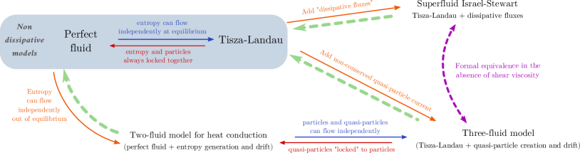
Figure 1: Some fluid models related to our superfluid version of Israel-Stewart hydrodynamics (equivalent to the Carter’s three-fluid model developed in this work). The dashed green arrows indicate the evolution of the dissipative models towards the corresponding non-dissipative limit as the fluid naturally relaxes to equilibrium. On the other hand, to upgrade the non-dissipative model to a dissipative one, new degrees of freedom are introduced. For example, promoting all the components of the entropy current to independent degrees of freedom leads to Carter’s two-fluid model for heat conducting fluids developed in Carter (1989); Lopez-Monsalvo and Andersson (2011). Similarly, adding a non-conserved quasi-particle current to the relativistic version of the Tisza-Landau model – Carter’s dissipationless two-fluid model, see e.g. (Gavassino and Antonelli, 2020) – provides a way to construct the superfluid version of Israel-Stewart hydrodynamics via the multifluid approach.

It is well known that a relativistic version of the Tisza-Landau two-fluid model of a simple superfluid (e.g., Helium-II) can be rewritten as a Carter multifluid with two currents: particles and entropy. However, such a theory is valid in the non-dissipative limit. In order to account for dissipation coming from heat conduction and bulk viscosity we add another non-conserved current (that we interpret as the current of quasi-particles) to the Tisza-Landau model, similarly to the fact that to model heat conduction in a normal fluid one can modify the perfect fluid by promoting the entropy current to a new degree of freedom (Carter, 1989; Lopez-Monsalvo and Andersson, 2011), see Figure 1.

The final result is a fully relativistic hydrodynamic description of a superfluid, where dissipation is linked to the presence of quasi-particle reactions (bulk viscosity) and to the fact that the quasi-particles do not necessarily comove with the entropy flow (heat conduction).

We also perform a change of variables (from currents to dissipative fluxes) and a perturbative expansion near local thermodynamic equilibrium to translate our multifluid model into its Israel-Stewart counterpart. We use this equivalent Israel-Stewart formulation to verify that the infrared Eckart-type limit of our three-fluid hydrodynamics is the superfluid model of Gusakov (2007).

Throughout the paper we adopt the spacetime signature $(-,+,+,+)$ and work in natural units $c=G=k_{B}=1$. The Planck constant is $h_{p}=2\pi\hbar$.

II Three currents fluid

In this section we derive the constitutive relations (Gavassino and Antonelli, 2021) of the model directly from the variational approach of Carter and Khalatnikov (1992). The superfluid will be assumed to be Bosonic; extensions of the model beyond this assumption will be presented in section X.

II.1 Fundamental variables: relation between Carter and Israel-Stewart formulations

Let $n^{\nu}$ be the conserved particle current of the superfluid,

$$\nabla_{\nu}n^{\nu}=0\,,$$ (1)

and $s^{\nu}$ the entropy current density (Sha, 1975), which obeys to the second law of thermodynamics (Israel, 2009):

$$\nabla_{\nu}s^{\nu}\geq 0\,.$$ (2)

We keep track of the evolution of the elementary excitations in the superfluid phase by introducing an additional quasi-particle current $z^{\nu}$, which is not conserved

$$\nabla_{\nu}z^{\nu}\neq 0\,,$$ (3)

because reactions of the type (the superfluid is Bosonic)

$$z+z\ce{<=>}z+z+z$$ (4)

are allowed (Khalatnikov, 1965). For simplicity, we assume that all the quasi-particles are of only one kind $z$. In the case that two or more species of quasi-particles are present (such as phonons and rotons in ⁴He), it would be possible to construct a slightly different theory, as discussed in subsection X.1.

If every volume element of the superfluid is in LTE, the two currents $n^{\nu}$ and $s^{\nu}$ are all the information needed to identify the local thermodynamic state (Carter and Langlois, 1995). This implies that $z^{\nu}$ is not an independent field, but it is given in every point by an equilibrium constitutive relation of the kind

$$z^{\nu}=z_{\text{eq}}^{\nu}(n^{\rho},s^{\rho})\,.$$ (5)

When dissipative processes are at work, the fluid elements can also explore macrostates that are out of equilibrium. Contrarily to what happens in the non-relativistic Navier-Stokes hydrodynamics, in a relativistic framework this leads necessarily to an enlargement of the number of degrees of freedom of the dissipative hydrodynamic model (Gavassino et al., 2020a; Gavassino and Antonelli, 2021): since we aim to describe bulk viscosity and heat conduction, we need to include at least 4 new independent algebraic degrees of freedom, the scalar viscous stress $\Pi$ and the heat flux $Q^{\nu}$. Treating these dissipative fluxes as independent variables would directly lead us to an Israel-Stewart-type model. We prefer, however, the more deductive approach of Carter, but first we have to identify its natural variables. To move from the independent degrees of freedom $n^{\rho}$, $s^{\rho}$, $\Pi$ and $Q^{\nu}$ of an Israel-Stewart model to those of Carter’s approach, we need to perform a change of variables, as outlined below.

Assume that $n^{\rho}$, $s^{\rho}$, $\Pi$ and $Q^{\rho}$ are the full set of algebraically independent variables (Gavassino and Antonelli, 2021) of an Israel-Stewart-type model. Hence, there must be a non-equilibrium constitutive relation that generalizes (5),

$$z^{\nu}=z^{\nu}(n^{\rho},s^{\rho},\Pi,Q^{\rho})\,,$$ (6)

where, since in equilibrium $\Pi=Q^{\rho}=0$, the functions in (5) and (6) are related by the condition

$$z^{\nu}(n^{\rho},s^{\rho},0,0)=z_{\text{eq}}^{\nu}(n^{\rho},s^{\rho})\,.$$ (7)

Since the components of $z^{\nu}$ are 4, we can assume that it is possible to invert the relation (6) to obtain

$$\Pi=\Pi(n^{\rho},s^{\rho},z^{\rho})\quad\quad\quad Q^{\nu}=Q^{\nu}(n^{\rho},s^{\rho},z^{\rho})\,.$$ (8)

This allows us to make the desired change of variables:

$$(n^{\rho},s^{\rho},\Pi,Q^{\rho})\longrightarrow(n^{\rho},s^{\rho},z^{\rho})\,.$$ (9)

Now that the degrees of freedom are 3 independent four-currents, it is possible to model the system using the approach of Carter and Khalatnikov (1992), which is entirely based on currents: we have shown that bulk viscosity and heat conduction in a superfluid can be implemented by promoting the four-current of quasi-particles to an independent current of the theory. This is a generalization to superfluid systems of the multifluid models proposed by Carter (1989) for heat conduction and in (Gavassino et al., 2021a) for bulk viscosity.

II.2 Advantages of a three currents formulation à-la Carter

Before moving on with the general discussion it is worth commenting on the advantages of a formulation based on three currents with respect to an Israel-Stewart model.

In the Israel-Stewart framework, the dissipative fluxes $\Pi$ and $Q^{\rho}$ are defined as deviations from a reference value (typically zero) that is attained at thermodynamic equilibrium. This implies that a formalism based on the dissipative fluxes is structurally perturbative. On the other hand, a theory based on the physical currents $n^{\rho},s^{\rho}$ and $z^{\rho}$ – which can be also defined arbitrarily far from equilibrium through kinetic theory (Khalatnikov, 1965; Popov, 2006) – does not need to make explicit reference of an equilibrium state in the constitutive relations. Clearly, for this hydrodynamic model to have physical significance, in the end one needs to impose a near-equilibrium assumption, but this is not directly encoded into the mathematical structure of the equations: Carter’s theory does not invoke any separation between an equilibrium and a non-equilibrium part. This makes the formalism easier to handle, and independent from the problem of the choice of a so-called hydrodynamic frame (Kovtun, 2019), at least at the level of the constitutive relations.

II.3 Carter’s prescription for the energy-momentum tensor

Following Carter and Khalatnikov (1992), we assume that all the information about the state of the fluid is contained in a hydrodynamic scalar field $\Lambda$. By Lorentz invariance, $\Lambda$ can be written as a function of the local Lorentz scalars of the fluid:

$$\Lambda=\Lambda(n^{2},s^{2},z^{2},n_{ns}^{2},n_{nz}^{2},n_{sz}^{2}),$$ (10)

where

$$n^{2}=-n^{\nu}n_{\nu}\quad\quad\quad s^{2}=-s^{\nu}s_{\nu}\quad\quad\quad z^{2}=-z^{\nu}z_{\nu}$$ (11)

and

$$n_{ns}^{2}=-n^{\nu}s_{\nu}\quad\quad\quad n_{nz}^{2}=-n^{\nu}z_{\nu}\quad\quad\quad n_{sz}^{2}=-s^{\nu}z_{\nu}.$$ (12)

The infinitesimal variation of (10) has the form

$$\begin{split}\delta\Lambda=&-\dfrac{Y^{-1}}{2}\,\delta(n^{2})-\dfrac{\mathcal{C}}{2}\,\delta(s^{2})-\dfrac{\mathcal{B}^{z}}{2}\,\delta(z^{2})\\ &-\mathcal{A}^{ns}\,\delta(n_{ns}^{2})-\mathcal{A}^{nz}\,\delta(n_{nz}^{2})-\mathcal{A}^{sz}\,\delta(n_{sz}^{2}).\\ \end{split}$$ (13)

It is convenient to introduce the chemical labels $x,y$ which run over $n,s,z$ and the symmetric $3\times 3$ entrainment matrix

$$\mathcal{K}^{xy}=\begin{bmatrix}Y^{-1}&\mathcal{A}^{ns}&\mathcal{A}^{nz}\\ \mathcal{A}^{ns}&\mathcal{C}&\mathcal{A}^{sz}\\ \mathcal{A}^{nz}&\mathcal{A}^{sz}&\mathcal{B}^{z}\\ \end{bmatrix}\,,$$ (14)

that can be used to rewrite the differential (13) in the more compact form (Carter and Khalatnikov, 1992)

$$\delta\Lambda=\dfrac{1}{2}\sum_{x,y}\mathcal{K}^{xy}\delta(n_{x}^{\nu}n_{y\nu})\,.$$ (15)

Assuming that the variation is arbitrary (involving also the metric), we can make the substitution

$$\delta(n_{x}^{\nu}n_{y\nu})=n_{x\nu}\delta n_{y}^{\nu}+n_{y\nu}\delta n_{x}^{\nu}+n_{x}^{\nu}n_{y}^{\rho}\delta g_{\nu\rho}\,,$$ (16)

which allows us to rewrite (15) as

$$\delta\Lambda=\sum_{x}\bigg{(}\mu^{x}_{\nu}\delta n_{x}^{\nu}+\dfrac{1}{2}n_{x}^{\nu}\mu^{x\rho}\,\delta g_{\nu\rho}\bigg{)}\,,$$ (17)

where we have introduced the canonical momenta

$$\mu^{x}_{\nu}=\sum_{y}\mathcal{K}^{xy}n_{y\nu}\,.$$ (18)

In what follows, we adopt the more physical names for the momenta

$$\mu_{\nu}^{n}=\mu_{\nu}\quad\quad\quad\mu^{s}_{\nu}=\Theta_{\nu}\quad\quad\quad\mu^{z}_{\nu}=-\mathbb{A}_{\nu}\,,$$ (19)

and we call $\mu_{\nu}$, $\Theta_{\nu}$ and $\mathbb{A}_{\nu}$ respectively chemical, thermal and affinity momentum (Gavassino and Antonelli, 2020; Gavassino et al., 2021a). In this way, equation (18) explicitly reads

$$\begin{split}&\mu_{\nu}=Y^{-1}n_{\nu}+\mathcal{A}^{ns}s_{\nu}+\mathcal{A}^{nz}z_{\nu}\\ &\Theta_{\nu}=\mathcal{A}^{ns}n_{\nu}+\mathcal{C}s_{\nu}+\mathcal{A}^{sz}z_{\nu}\\ -&\mathbb{A}_{\nu}=\mathcal{A}^{nz}n_{\nu}+\mathcal{A}^{sz}s_{\nu}+\mathcal{B}^{z}z_{\nu}\,.\\ \end{split}$$ (20)

The coefficients $\mathcal{A}^{xy}$ are responsible for the non-collinearity between the currents and the respective momenta (for this reason they are sometimes called “anomalies”, or “entrainment” coefficients).

The central postulate of Carter’s approach is that all the components of the stress-energy tensor $T^{\nu\rho}$, which obeys the conservation law

$$\nabla_{\nu}T^{\nu\rho}=0,$$ (21)

can be computed directly from $\Lambda$ by using the prescription

$$T^{\nu\rho}=\dfrac{2}{\sqrt{|g|}}\dfrac{\partial(\sqrt{|g|}\Lambda)}{\partial g_{\nu\rho}}\bigg{|}_{\sqrt{|g|}\,n_{x}^{\sigma}},$$ (22)

where $\sqrt{|g|}$ is the square root of the absolute value of the determinant of the metric. The partial derivative appearing on the right-hand side of (22) can be computed explicitly from the differential (17), giving

$$T\indices{{}^{\nu}_{\rho}}=\Psi\delta\indices{{}^{\nu}_{\rho}}+n^{\nu}\mu_{\rho}+s^{\nu}\Theta_{\rho}-z^{\nu}\mathbb{A}_{\rho}\,,$$ (23)

where $\delta\indices{{}^{\nu}_{\rho}}=g\indices{{}^{\nu}_{\rho}}$ is the identity tensor, and

$$\Psi=\Lambda-n^{\nu}\mu_{\nu}-s^{\nu}\Theta_{\nu}+z^{\nu}\mathbb{A}_{\nu}$$ (24)

can be interpreted as a generalized pressure.

There is consensus on the idea of using an equation of the kind (22) to prescribe the energy-momentum tensor for a superfluid in the non-dissipative limit (Carter and Khalatnikov, 1992; Andersson and Comer, 2007). This may be justified in view of the formal equivalence between this phenomenological approach and the more fundamental derivations of superfluid hydrodynamics proposed by Lebedev and Khalatnikov (1982); Son (2001); Gusakov (2016), referred to as “LAB” in (Gavassino and Antonelli, 2020). However, it is not guaranteed that it’s possible to extrapolate this principle to a dissipative context. Although we do not provide a rigorous derivation of (22) from kinetic theory, in the following we will show that the predictions made by using a dissipative model based on (22) are substantially indistinguishable from those of a hypothetical “exact” theory.

II.4 Landau representation

The system we have presented in the previous subsection describes a generic three-component multifluid. To make contact with the physics of superfluids we need to connect it to Landau’s dissipative two-fluid model. Generalizing what has been done in the non-dissipative theory by Carter and Langlois (1995), we postulate that

$$\mu_{\nu}=\hbar\,\nabla_{\nu}\phi\,,$$ (25)

where $\phi$ is the gradient of the phase of the order parameter and $\hbar$ is the reduced Planck’s constant. Equation (25) leads to the irrotationality condition

$$\nabla_{[\rho}\mu_{\nu]}=0\,.$$ (26)

Thus, also in the present dissipative scheme, the chemical momentum $\mu_{\nu}$ is the relativistic generalization of the Landau’s superfluid velocity (within an overall constant which in the Newtonian limit coincides with the mass of the constituents).

In the usual hydrodynamic description of Newtonian superfluids, the so-called superfluid velocity (in our case the chemical momentum $\mu_{\nu}$) is treated as a primary degree of freedom, leading to a particular case of hybrid (or “mongrel”) representation where some variables are momenta and some are currents (Prix, 2000; Gavassino and Antonelli, 2020). Thus, to explore the bridge with the Landau theory and its relativistic “LAB” extension, it is useful to make the change of variables (compare with (Carter and Langlois, 1995))

$$(n^{\rho},s^{\rho},z^{\rho})\longrightarrow(\mu_{\rho},s^{\rho},z^{\rho})$$ (27)

and, consequently, to write $n^{\nu}$, $\Theta_{\nu}$ and $\mathbb{A}_{\nu}$ as linear combinations of $\mu_{\nu},$ $s^{\nu}$ and $z^{\nu}$. To do this we invert the first equation of (20), obtaining

$$n^{\nu}=Y\mu^{\nu}-\mathcal{D}^{ns}s^{\nu}-\mathcal{D}^{nz}z^{\nu}\,,$$ (28)

where we have defined the coefficients

$$\mathcal{D}^{ns}=Y\mathcal{A}^{ns}\quad\quad\quad\mathcal{D}^{nz}=Y\mathcal{A}^{nz}\,.$$ (29)

Then, the second and the third equations of (20) become

$$\begin{split}&\Theta_{\nu}=\mathcal{D}^{ns}\mu_{\nu}+\mathcal{M}^{ss}s_{\nu}+\mathcal{M}^{sz}z_{\nu}\\ -&\mathbb{A}_{\nu}=\mathcal{D}^{nz}\mu_{\nu}+\mathcal{M}^{sz}s_{\nu}+\mathcal{M}^{zz}z_{\nu}\,,\\ \end{split}$$ (30)

with

$$\begin{split}&\mathcal{M}^{ss}=\mathcal{C}-Y(\mathcal{A}^{ns})^{2}\\ &\mathcal{M}^{zz}=\mathcal{B}^{z}-Y(\mathcal{A}^{nz})^{2}\\ &\mathcal{M}^{sz}=\mathcal{A}^{sz}-Y\mathcal{A}^{ns}\mathcal{A}^{nz}\,.\\ \end{split}$$ (31)

The formulas (28) and (30) can be represented in the more compact form

$$\begin{pmatrix}-n^{\nu}\\ \Theta^{\nu}\\ -\mathbb{A}^{\nu}\\ \end{pmatrix}=\begin{bmatrix}-Y&\mathcal{D}^{ns}&\mathcal{D}^{nz}\\ \mathcal{D}^{ns}&\mathcal{M}^{ss}&\mathcal{M}^{sz}\\ \mathcal{D}^{nz}&\mathcal{M}^{sz}&\mathcal{M}^{zz}\\ \end{bmatrix}\begin{pmatrix}\mu^{\nu}\\ s^{\nu}\\ z^{\nu}\\ \end{pmatrix},$$ (32)

which is the analogue of (18), written in terms of the new degrees of freedom of the “LAB” description.

It is useful to know that all the coefficients of the $3\times 3$ symmetric matrix introduced in (32) can be obtained as partial derivatives of a function $\mathcal{X}$, just as the entrainment matrix $\mathcal{K}^{xy}$ can be computed directly from $\Lambda$. To show this, we write explicitly the differential (17) working at fixed metric components (i.e., imposing $\delta g_{\nu\rho}=0$):

$$\delta\Lambda=\mu_{\nu}\delta n^{\nu}+\Theta_{\nu}\delta s^{\nu}-\mathbb{A}_{\nu}\delta z^{\nu}\,.$$ (33)

We can implement the change of variables (27) by defining the new quantity $\mathcal{X}$ as the Legendre transform of $\Lambda$ with respect to $n^{\nu}$,

$$\mathcal{X}=\Lambda-\mu_{\nu}n^{\nu}\,.$$ (34)

Therefore, $\mathcal{X}$ contains the same amount information as $\Lambda$ (Callen, 1985), and its variation is

$$\delta\mathcal{X}=-n^{\nu}\delta\mu_{\nu}+\Theta_{\nu}\delta s^{\nu}-\mathbb{A}_{\nu}\delta z^{\nu}\,.$$ (35)

Analogously to (10), we can write $\mathcal{X}$ as a function of 6 local scalars:

$$\mathcal{X}=\mathcal{X}(\mu^{2},s^{2},z^{2},y_{ns}^{2},y_{nz}^{2},n_{sz}^{2})\,,$$ (36)

where

$$\mu^{2}=-\mu^{\nu}\mu_{\nu}\quad\quad\quad y_{ns}^{2}=-\mu_{\nu}s^{\nu}\quad\quad\quad y_{nz}^{2}=-\mu_{\nu}z^{\nu}.$$ (37)

With steps which are analogous to those which led us from (15) to (17), it’s possible to show that the only way for (36) to be consistent with (32) is that the infinitesimal variation of (36) is given by

$$\begin{split}\delta\mathcal{X}=&+\dfrac{Y}{2}\,\delta(\mu^{2})-\dfrac{\mathcal{M}^{ss}}{2}\,\delta(s^{2})-\dfrac{\mathcal{M}^{zz}}{2}\,\delta(z^{2})\\ &-\mathcal{D}^{ns}\,\delta(y_{ns}^{2})-\mathcal{D}^{nz}\,\delta(y_{nz}^{2})-\mathcal{M}^{sz}\,\delta(n_{sz}^{2})\,.\\ \end{split}$$ (38)

Thus, we have shown that, to compute all the coefficients appearing in the Landau representation, it is enough to know the thermodynamic potential $\mathcal{X}$.

Finally, we can rewrite the energy-momentum tensor of the superfluid in the Landau representation. Introducing the “chemical” labels $A,B\in\{s,z\}$, equation (23) can be recast into the form

$$T^{\nu\rho}=\Psi g^{\nu\rho}+Y\mu^{\nu}\mu^{\rho}+n_{A}^{\nu}\mathcal{M}^{AB}n_{B}^{\rho}\,.$$ (39)

In this representation the superfluid and normal contributions to the stress-energy tensor are automatically separated. This also shows that $Y$ is the relativistic generalization of the Landau’s superfluid density, within a square-mass factor (Carter and Langlois, 1995).

II.5 The generating function approach

Carter’s approach is constructed as a variational approach, where the scalar field $\Lambda$ plays the role of the Lagrangian density of the matter sector. This point of view is very convenient when one is dealing with a non-dissipative system, because it produces the full set of equations of the system (including both the constitutive relations and the field equations), see e.g. (Carter and Khalatnikov, 1992; Carter and Langlois, 1995; Gavassino and Antonelli, 2020) and references therein.

However, in a dissipative context one is usually forced to rely on an “incomplete” variational approach, where the constitutive relations are derived from the action principle, while the dissipative hydrodynamic equations are “guessed” by appropriately modifying the (non-dissipative) Euler-Lagrange equations (Carter, 1989, 1991; Langlois et al., 1998). This converts the scalar field $\Lambda$ into a sort of “generating function” for the dissipative theory, namely a function which can be used to compute all the relevant tensors of the theory as partial derivatives but that does not contain the whole information needed to write down the full dynamics.

Within this “generating function” point of view, all the equations of this entire section can be summarised into two fundamental relations:

$$\begin{split}&\Lambda=T\indices{{}^{\nu}_{\nu}}-3\Psi\\ &\dfrac{\delta(\sqrt{|g|}\,\Lambda)}{\sqrt{|g|}}=\sum_{x}\mu^{x}_{\nu}\dfrac{\delta(\sqrt{|g|}\,n_{x}^{\nu})}{\sqrt{|g|}}+\dfrac{T^{\nu\rho}}{2}\,\delta g_{\nu\rho}\,,\\ \end{split}$$ (40)

which can be proved combining (17), (22), (23) and (24), but they are also true for a generic multi-fluid constructed using Carter’s approach.

The first equation in (40) tells us that the scalar field $\Lambda$ is not just a mathematical device. Instead, it is a physical observable, which is uniquely determined for a given fluid, independently from which choice of degrees of freedom we make. In particular, $-\Lambda$, $-\Psi$ and $-\mathcal{X}$ are thermodynamic potentials, that are all linked to the internal energy via Legendre transform, see (Gavassino and Antonelli, 2020).

The second equation in (40) collects together all the relevant constitutive relations in a single differential,

$$\begin{split}\dfrac{\delta(\sqrt{|g|}\,\Lambda)}{\sqrt{|g|}}=&\,\mu_{\nu}\dfrac{\delta(\sqrt{|g|}\,n^{\nu})}{\sqrt{|g|}}+\Theta_{\nu}\dfrac{\delta(\sqrt{|g|}\,s^{\nu})}{\sqrt{|g|}}\\ &-\mathbb{A}_{\nu}\dfrac{\delta(\sqrt{|g|}\,z^{\nu})}{\sqrt{|g|}}+\dfrac{T^{\nu\rho}}{2}\,\delta g_{\nu\rho}\,.\\ \end{split}$$ (41)

This formula will be useful later, as it allows us to keep track directly of all the transformations that occur whenever we decide to make a change of degrees of freedom.

To give an idea of how this works in practice, we consider the following application: if one works in the Landau representation (which we introduced in the previous subsection), is there an analogue of equation (22) for computing $T^{\mu\nu}$ directly from $\mathcal{X}$? The answer is yes: first, we use (34) to prove the identity

$$\dfrac{\delta(\sqrt{|g|}\,\mathcal{X})}{\sqrt{|g|}}=\dfrac{\delta(\sqrt{|g|}\,\Lambda)}{\sqrt{|g|}}-\mu_{\nu}\dfrac{\delta(\sqrt{|g|}\,n^{\nu})}{\sqrt{|g|}}-n^{\nu}\delta\mu_{\nu}.$$ (42)

Then, from (41) we obtain

$$\begin{split}\dfrac{\delta(\sqrt{|g|}\,\mathcal{X})}{\sqrt{|g|}}=&\,-n^{\nu}\delta\mu_{\nu}+\Theta_{\nu}\dfrac{\delta(\sqrt{|g|}\,s^{\nu})}{\sqrt{|g|}}\\ &-\mathbb{A}_{\nu}\dfrac{\delta(\sqrt{|g|}\,z^{\nu})}{\sqrt{|g|}}+\dfrac{T^{\nu\rho}}{2}\,\delta g_{\nu\rho}\,,\\ \end{split}$$ (43)

which implies that the analogous of (22) is

$$T^{\nu\rho}=\dfrac{2}{\sqrt{|g|}}\dfrac{\partial(\sqrt{|g|}\mathcal{X})}{\partial g_{\nu\rho}}\bigg{|}_{\mu_{\sigma}\,,\,\sqrt{|g|}\,s^{\sigma}\,,\,\sqrt{|g|}\,z^{\sigma}}\,.$$ (44)

Indeed, if one takes the generic variation (38), and uses it to compute the partial derivative (44), they obtain directly the formula (39) for the stress-energy tensor, see Appendix A.1 for the proof. This result (which is straightforward in a generating function approach) is at the origin of the equivalence between the potential (Lebedev and Khalatnikov, 1982), the convective (Carter and Khalatnikov, 1992) and the hybrid (Carter and Langlois, 1995) variational derivations of covariant superfluid dynamics (Carter and Khalatnikov, 1992).

II.6 Field equations

Now that the constitutive relations and a physical interpretation of the hydrodynamic fields have been fixed, we need to derive the field equations (Gavassino and Antonelli, 2021). It is possible to show that (see, e.g., equation (141) in (Gavassino and Antonelli, 2020))

$$\nabla_{\nu}T\indices{{}^{\nu}_{\rho}}=\mathcal{R}^{n}_{\rho}+\mathcal{R}^{s}_{\rho}+\mathcal{R}^{z}_{\rho}\,,$$ (45)

where the canonical hydrodynamic forces $\mathcal{R}^{x}_{\rho}$ are

$$\begin{split}&\mathcal{R}^{n}_{\rho}=2n^{\nu}\nabla_{[\nu}\mu_{\rho]}+\mu_{\rho}\nabla_{\nu}n^{\nu}\\ &\mathcal{R}^{s}_{\rho}=2s^{\nu}\nabla_{[\nu}\Theta_{\rho]}+\Theta_{\rho}\nabla_{\nu}s^{\nu}\\ &\mathcal{R}^{z}_{\rho}=-2z^{\nu}\nabla_{[\nu}\mathbb{A}_{\rho]}-\mathbb{A}_{\rho}\nabla_{\nu}z^{\nu}\,.\\ \end{split}$$ (46)

From the conservation (1) and irrotationality (26) conditions, we obtain

$$\mathcal{R}^{n}_{\rho}=0\,.$$ (47)

Therefore, recalling (21), equation (45) implies

$$\mathcal{R}^{z}_{\rho}=-\mathcal{R}^{s}_{\rho}.$$ (48)

Now, let us see how many equations are needed to close the system. The model builds on 3 independent four-currents, so it has $4+4+4=12$ algebraic degrees of freedom. The energy-momentum conservation gives 4 equations and the particle conservation 1. The irrotationality conditions (26) are 6 equations, however 3 of them are constraints on the initial conditions, therefore only 3 are proper equations of motion. Thus, we have a total of 4+1+3=8 hydrodynamic equations. We need other 12-8=4 equations to close the system: to complete the model we only need to give a prescription for the four-force $\mathcal{R}^{s}_{\rho}$ from kinetic theory. It has been shown that, in general, there is in no universal prescription for the structure of a force of this kind (Gavassino et al., 2020b). In fact, this force may, or may not, involve derivatives of the hydrodynamic fields and it cannot be constrained further using purely geometrical and thermodynamic arguments.

Following the approach of Carter (1989), in section VII we will choose the simplest possible prescription for $\mathcal{R}^{s}_{\rho}$, which contains all the physics we need. With this specific construction, we will have at our disposal a minimal model for bulk viscosity and heat conduction. However, before making this choice, it is convenient to see what we can conclude on general grounds, without selecting any particular formula for $\mathcal{R}^{s}_{\rho}$.

III Out-of-equilibrium evolution of homogeneous states

A common feature of relativistic hydrodynamic theories for dissipation is the existence of a dynamical evolution also in the homogeneous limit (in which the spatial gradients are zero), which manifests itself in the existence of gapped dispersion relations in the spectrum of the linear theory (Kovtun, 2019). Within UEIT, this intrinsic evolution is interpreted as the point of contact of the model with non-equilibrium thermodynamics (Gavassino and Antonelli, 2021). Therefore, it is important to see how the present hydrodynamic model behaves in the homogeneous limit, as this is the configuration in which the bridge with statistical mechanics must become evident (Gavassino and Antonelli, 2020).

Throughout this section, we will assume that the space-time is Minkowski and that all the states under consideration (both the perturbed and the unperturbed ones) are homogeneous in the adopted global inertial frame.

III.1 Equilibration dynamics and equilibrium conditions

Our first task is to see if the fluid admits a homogeneous equilibrium state, and if the properties of this state are consistent with microphysics.

We start from the observation that in the homogeneous limit equations (1), (2), (21) and (25) take the simpler form

$$\partial_{t}n^{0}=0\quad\quad\partial_{t}s^{0}\geq 0\quad\quad\partial_{t}T^{0\rho}=0\quad\quad\partial_{t}\mu_{j}=0\,.$$ (49)

If we find a state that maximize $s^{0}$ at constant particle density, energy-momentum per unit volume and spatial part of the superfluid momentum, then this is necessarily an equilibrium state of the system and, since $s^{0}$ can only grow or stay constant, it is automatically a Lyapunov-stable equilibrium (Gavassino et al., 2020a; Gavassino and Antonelli, 2021).

Let $\varphi$ and $\varphi+\delta\varphi$ be the values of a generic observable ($\varphi$, in this example) respectively at equilibrium and in a perturbed state; both states are homogeneous. Then, the first-order variation of (23) reads (the metric is fixed)

$$\delta T\indices{{}^{\nu}_{\rho}}=\delta\indices{{}^{\nu}_{\rho}}\,\delta\Psi+\sum_{x}(\mu^{x}_{\rho}\delta n_{x}^{\nu}+n_{x}^{\nu}\delta\mu^{x}_{\rho})\,.$$ (50)

Considering that equation (24) can be written in the compact form

$$\Psi=\Lambda-\sum_{x}n_{x}^{\nu}\mu^{x}_{\nu}\,,$$ (51)

the variation $\delta\Psi$, recalling (17), is

$$\delta\Psi=-\sum_{x}n_{x}^{\nu}\delta\mu^{x}_{\nu}\,.$$ (52)

So, contracting equation (50) with the inverse-temperature vector (Carter and Langlois, 1995; Becattini, 2016) (not to be confused with the thermal covector $\Theta_{\nu}$)

$$\beta^{\rho}:=-s^{\rho}/(\Theta_{\lambda}s^{\lambda})\,,$$ (53)

we obtain

$$\beta^{\rho}\delta T\indices{{}^{\nu}_{\rho}}=\sum_{x}\bigg{(}\beta^{\rho}\mu^{x}_{\rho}\delta n_{x}^{\nu}+2n_{x}^{[\nu}\beta^{\rho]}\delta\mu^{x}_{\rho}\bigg{)}.$$ (54)

From the definition (53) it follows

$$\beta^{\rho}\Theta_{\rho}=-1\quad\quad\quad s^{[\nu}\beta^{\rho]}=0\,,$$ (55)

so that we can isolate the variation of the entropy current in (54), obtaining

$$\begin{split}\delta s^{\nu}=&-\beta_{\rho}\delta T^{\nu\rho}+\beta^{\rho}\mu_{\rho}\delta n^{\nu}-\beta^{\rho}\mathbb{A}_{\rho}\delta z^{\nu}+\\ &+2n^{[\nu}\beta^{\rho]}\delta\mu_{\rho}-2z^{[\nu}\beta^{\rho]}\delta\mathbb{A}_{\rho}\,.\\ \end{split}$$ (56)

We need to maximize $s^{0}$ at constant particle density, energy-momentum per unit volume and spatial part of the superfluid momentum (Gavassino and Antonelli, 2020). Thus, taking the component $\nu=0$ of equation (56) and imposing

$$\delta T^{0\rho}=0\quad\quad\quad\delta n^{0}=0\quad\quad\quad\delta\mu_{j}=0\,,$$ (57)

we have to set to zero the variation

$$\delta s^{0}=-\beta^{\rho}\mathbb{A}_{\rho}\delta z^{0}-2z^{[0}\beta^{\rho]}\delta\mathbb{A}_{\rho}=0\,.$$ (58)

This provides 4 equilibrium conditions, which allow us to find the functions $z_{\text{eq}}^{\nu}(n^{\rho},s^{\rho})$ introduced in equation (5). Imposing the stationarity with respect to processes of quasi-particle creation and annihilation, associated with the variation $\delta z^{0}$ in (58), we obtain the chemical equilibrium condition

$$s^{\rho}\mathbb{A}_{\rho}=0\,.$$ (59)

This is simply the requirement that the affinity of the reaction (4), as measured in the frame of the entropy (Gavassino and Antonelli, 2020), vanishes. Therefore, we have shown that the model predicts that the chemical potential of the quasi-particles in equilibrium is zero, in agreement with the statistical mechanics of a superfluid (Khalatnikov, 1965).

Imposing the stationarity of $s^{0}$ with respect to variations of the momentum per-quasi-particle $\mathbb{A}_{j}$, we obtain from (58) the collinearity condition

$$z^{[\nu}s^{\rho]}=0\,.$$ (60)

We have found that in thermodynamic equilibrium the quasi-particle current is locked to the entropy current, or, in other words, the entropy is transported by the excitations, in agreement with the Landau theory of superfluidity (Landau and Lifshitz, 2013a), see equations (8-24), (21-3) and (21-4) of Khalatnikov (1965). The two equilibrium conditions (59) and (60) are also in accordance with the derivation of the thermodynamics of a generic multifluid presented in (Gavassino and Antonelli, 2020).

We remark that we have not verified under which conditions the state given by equations (59) and (60) is a real maximum of the entropy, and not just a saddle point or a minimum. Addressing this issue would lead us to a stability analysis of the kind performed by Hiscock and Lindblom (1983) for normal Israel-Stewart fluids, producing several thermodynamic inequalities for the equation of state (10). Such inequalities generalise the Gibbs stability criterion to superfluid systems (Prigogine, 1968; Andreev and Melnikovsky, 2004; Gavassino et al., 2020a; Gavassino, 2021a; Gavassino et al., 2021b). This analysis is beyond the scope of the present paper, but it will be addressed in future work.

III.2 Thermodynamics of the three-current model

It is interesting to analyse in more detail the properties of the equilibrium states. To do so, let us restrict the generic differential (56) to equilibrium configurations: we have to impose the two equilibrium conditions (59) and (60), obtaining

$$\delta s^{\nu}=-\beta_{\rho}\delta T^{\nu\rho}+\beta^{\rho}\mu_{\rho}\delta n^{\nu}+2n^{[\nu}\beta^{\rho]}\delta\mu_{\rho}\,.$$ (61)

This is the thermodynamic differential of a relativistic superfluid in local thermodynamic equilibrium proposed by Lebedev and Khalatnikov (1982), see equation (43) therein. In addition, in Appendix A.2 we prove that the Newtonian limit of this differential, for $\nu=0$, is equation (4) of Andreev and Melnikovsky (2004), which constitutes the Galilean-covariant thermodynamic differential of a Newtonian superfluid.

Equation (61) is naturally presented in a form which reminds us of the covariant Gibbs relation given by Israel in (Israel, 2009), which we will refer to from now on as Israel’s covariant Gibbs relation, including, however, a further term $2n^{[\nu}\beta^{\rho]}\delta\mu_{\rho}$ associated with the variation of the superfluid momentum. Indeed, if the irrotationality constraint (26) did not hold, then we would not be allowed to impose the conservation law $\partial_{t}\mu_{j}=0$ and we would obtain a further equilibrium condition

$$n^{[\nu}s^{\rho]}=0\,.$$ (62)

In this case, the superfluid and normal components move together and (61) would reduce exactly to Israel’s covariant Gibbs relation

$$\delta s^{\nu}=-\beta_{\rho}\,\delta T^{\nu\rho}+\beta^{\rho}\mu_{\rho}\,\delta n^{\nu}\,.$$ (63)

This shows that the possibility of having a relative motion between the superfluid and the normal component is only the result of the conservation of the superfluid momentum on very long timescales (or Landau superfluid velocity). In this sense, the states in which (62) does not hold may be considered as long-lived metastable states with an effectively infinite lifetime, which exist as a result of the presence of 3 constants of motion which break the ergodicity of the system (Gavassino and Antonelli, 2020; Gavassino, 2020). The unique state given by (62) would, in this case, be interpreted as the absolute equilibrium state fulfilling Israel’s covariant Gibbs relation exactly. In a hydrodynamic framework, since the conservation of $\mu_{j}$ is given as an exact constraint, it is more convenient to consider these metastable states as genuine equilibrium states and to regard (61) as an equilibrium thermodynamic differential, which includes the superfluid momenta as free variables (for a microscopic counterpart of this discussion see Huang (1987)).

This interpretation also allows us to extend the zeroth law of thermodynamics – when two bodies are in thermal equilibrium with each other, they have the same inverse-temperature vector (Gavassino, 2020) – to relativistic superfluid systems. Assume that the superfluid is weakly interacting with a homogeneous non-superfluid substance $H$, which carries no conserved charges and whose Israel’s Gibbs relation – compare with (61) – is

$$\delta s_{H}^{\nu}=-\beta_{\rho}^{H}\delta T^{\nu\rho}_{H}\,,$$ (64)

where $s^{\nu}_{H}$, $\beta_{\rho}^{H}$ and $T^{\nu\rho}_{H}$ are respectively the entropy current, inverse-temperature vector and energy-momentum tensor of $H$. We assume that

$$s_{\text{tot}}^{\nu}=s^{\nu}+s_{H}^{\nu}\quad\quad\quad T_{\text{tot}}^{\nu\rho}=T^{\nu\rho}+T_{H}^{\nu\rho}\,,$$ (65)

so that we can treat the substance $H$ as an ideal thermometer. The hydrodynamic evolution is, then, subject to the constraints

$$\partial_{t}n^{0}=0\quad\quad\partial_{t}\mu_{j}=0\quad\quad\partial_{t}T_{\text{tot}}^{0\rho}=0\quad\quad\partial_{t}s_{\text{tot}}^{0}\geq 0\,,$$ (66)

which implies that to find the maximum entropy state we need to maximize $s_{\text{tot}}^{0}$ imposing

$$\delta n^{0}=0\quad\quad\quad\delta\mu_{j}=0\quad\quad\quad\delta T^{0\rho}=-\delta T_{H}^{\nu\rho}\,.$$ (67)

This gives the equilibrium condition

$$\beta_{\rho}=\beta_{\rho}^{H}\,,$$ (68)

a result that generalizes the relativistic zeroth law to superfluid systems. In thermal equilibrium, the superfluid component is allowed to flow with respect to the thermometer, but the normal component is not. In fact, for the substance $H$ (which is not superfluid), it is in general true that

$$\beta_{\rho}^{H}=\dfrac{u_{H\rho}}{\Theta_{H}},$$ (69)

where $u_{H}^{\nu}$ is the fluid velocity of $H$ and $\Theta_{H}$ is its temperature. Therefore, the zeroth law (68) is equivalent to

$$s^{[\nu}u_{H}^{\rho]}=0\quad\quad\quad s^{\rho}\Theta_{\rho}=-s\,\Theta_{H}\,.$$ (70)

The first condition states that the normal component of the superfluid is subject to friction with the environment and has, therefore, a tendency to stick to it. The second equation is the rigorous definition of the temperature of the superfluid as the zeroth component of the thermal momentum measured in the normal rest-frame (in agreement with (Lebedev and Khalatnikov, 1982; Carter and Khalatnikov, 1992; Gavassino and Antonelli, 2020)).

IV Non-dissipative hydrodynamics

Let us move back to the inhomogeneous case, in an arbitrary spacetime. The next step of our study consists of verifying that our model admits the correct non-dissipative limit. We can use the two equations (59) and (60) to define the local thermodynamic equilibrium state of the fluid elements. Our task is to verify explicitly that, if we impose these conditions as dynamical restraints on the fluid motion, this gives rise to a non-dissipative hydrodynamic model ($\nabla_{\nu}s^{\nu}=0$). Furthermore, we aim to verify that the two-fluid model that emerges coincides with the one of Carter and Langlois (1995). The analysis is analogous to the one presented in section 4 of Carter and Khalatnikov (1992), apart from the fact that we prefer using a generating function approach.

IV.1 Reduction to a two-component model

First of all, we define precisely the physical setting we adopt to study the non-dissipative limit of the three-current model.

We consider a relativistic superfluid whose physical tensors can be computed via the generating function approach by using the model in section II. Assume that the processes driving the fluid elements to local thermodynamic equilibrium are so fast, compared to the time-scale of the hydrodynamic process under consideration, that the equilibrium conditions (59) and (60) are approximately valid on every space-time point. This means that we are in the so called equilibrium regime, see, e.g., subsection II-D in (Gavassino et al., 2021a). Then, we can impose that (5) is approximately valid everywhere,

$$z^{\nu}\approx z_{\text{eq}}^{\nu}(n^{\rho},s^{\rho})\,.$$ (71)

This reduces the algebraic degrees of freedom from 12 ($n^{\rho},s^{\rho},z^{\rho}$) to 8 ($n^{\rho},s^{\rho}$), producing a two-fluid model: our goal is to verify that the physical quantity $\Lambda=T\indices{{}^{\nu}_{\nu}}-3\Psi$ still plays the role of generating function for this two-fluid model.

First, we need to restrict the generic variation (41) to the state-space of the two-fluid model, which, according to the equilibrium condition (60), must satisfy a constraint of the form

$$z^{\nu}_{\mathrm{eq}}=y_{z}\,s^{\nu}\,.$$ (72)

The coefficient $y_{z}$ is a non-negative function of the local thermodynamic state,

$$y_{z}=y_{z}(n^{2},s^{2},n_{ns}^{2})\,,$$ (73)

and has to be solution of equation (59), to ensure local equilibrium with respect to quasi-particle production/annihilation processes. Thus, any term proportional to $\mathbb{A}_{\nu}s^{\nu}$ must vanish and we can impose

$$-\mathbb{A}_{\nu}\dfrac{\delta(\sqrt{|g|}\,z^{\nu}_{\mathrm{eq}})}{\sqrt{|g|}}=-y_{z}\mathbb{A}_{\nu}\dfrac{\delta(\sqrt{|g|}\,s^{\nu})}{\sqrt{|g|}},$$ (74)

which, plugged into (41), gives

$$\dfrac{\delta(\sqrt{|g|}\,\Lambda)}{\sqrt{|g|}}=\mu_{\nu}\dfrac{\delta(\sqrt{|g|}\,n^{\nu})}{\sqrt{|g|}}+\check{\Theta}_{\nu}\dfrac{\delta(\sqrt{|g|}\,s^{\nu})}{\sqrt{|g|}}+\dfrac{T^{\nu\rho}}{2}\,\delta g_{\nu\rho},$$ (75)

with

$$\check{\Theta}_{\nu}=\Theta_{\nu}-y_{z}\mathbb{A}_{\nu}.$$ (76)

Therefore, the restriction of $\Lambda$ to local thermodynamic equilibrium states produces, according to the prescription (40), the generating function of a two-component fluid with primary currents $n^{\nu}$ and $s^{\nu}$, having as conjugate momenta the covectors $\mu_{\nu}$ and $\check{\Theta}_{\nu}$, respectively. This implies that our definition of the superfluid momentum (25) reduces to the one of Carter and Langlois (1995) in local thermodynamic equilibrium. Furthermore, in local thermodynamic equilibrium

$$s^{\nu}\check{\Theta}_{\nu}=s^{\nu}\Theta_{\nu}\,,$$ (77)

which implies that the ordinary temperature of our three-component model coincides with the one of Carter and Khalatnikov (1992).

Finally, as a consequence of (75), the restriction of the stress-energy tensor (23) to the states of the two-fluid model must necessarily have the two-fluid canonical form

$$T\indices{{}^{\nu}_{\rho}}=\Psi\delta\indices{{}^{\nu}_{\rho}}+n^{\nu}\mu_{\rho}+s^{\nu}\check{\Theta}_{\rho}\,,$$ (78)

with generalised pressure

$$\Psi=\Lambda-n^{\nu}\mu_{\nu}-s^{\nu}\check{\Theta}_{\nu}\,.$$ (79)

This can also be verified explicitly.

In conclusion, we have shown that the constitutive relations of the two-fluid model of Carter and Langlois (1995) emerge directly from our three-component model if we impose the local thermodynamic equilibrium condition as a dynamical constraint. An analogous mechanism has also been discussed in detail in (Gavassino et al., 2020b).

IV.2 Entrainment coefficients of the non-dissipative theory

We can now obtain the entrainment coefficients (indicated with a hat) of the two-component model from the matrix (14) arising from our dissipative three-current model. We only need to plug (20) into (76), using the constraint (72) to get rid of $z^{\nu}$ as a degree of freedom:

$$\begin{split}&\mu_{\nu}=Y^{-1}n_{\nu}+(\mathcal{A}^{ns}+y_{z}\mathcal{A}^{nz})s_{\nu}\\ &\check{\Theta}_{\nu}=(\mathcal{C}+2y_{z}\mathcal{A}^{sz}+y_{z}^{2}\mathcal{B}^{z})s_{\nu}+(\mathcal{A}^{ns}+y_{z}\mathcal{A}^{nz})n_{\nu}.\\ \end{split}$$ (80)

This allows us to make the identifications

$$\check{\mathcal{B}}^{n}=Y^{-1}\quad\quad\quad\check{\mathcal{C}}=\mathcal{C}+2y_{z}\mathcal{A}^{sz}+y_{z}^{2}\mathcal{B}^{z}$$ (81)

and

$$\check{\mathcal{A}}^{ns}=\check{\mathcal{A}}^{sn}=\mathcal{A}^{ns}+y_{z}\mathcal{A}^{nz}.$$ (82)

Now, there is an interesting remark to make. Imagine a situation in which all the contributions coming from the entropy in the three-component model where negligibly small

$$\mathcal{C}\approx\mathcal{A}^{sz}\approx\mathcal{A}^{ns}\approx 0\,.$$ (83)

Then, we would have

$$\check{\mathcal{C}}\approx y_{z}^{2}\mathcal{B}^{z}\quad\quad\quad\check{\mathcal{A}}^{ns}=\check{\mathcal{A}}^{sn}\approx y_{z}\mathcal{A}^{nz}.$$ (84)

Since the quasi-particles are excitations carrying quanta of energy and momentum, the coefficients $\mathcal{B}^{z}$ and $\mathcal{A}^{nz}$ are in general non-negligible. This implies that, even in the case in which the entropy current constitutes a negligible contribution to the total energy-momentum balances, it acquires inertia in the two-component model, when the degrees of freedom are reduced and $z^{\nu}$ transfers its entrainment to $s^{\nu}$. This fact is the key to understand the connection of the non-dissipative theory of Carter with the Landau two-fluid model. In fact, in Newtonian physics, the entropy is always considered to be “massless”, in the sense that it does not carry rest-mass. However, in the Newtonian limit of Carter’s theory the entropy does contribute to the total mass current through the entrainment (Prix, 2004; Andersson and Comer, 2011). This arises from the fact that the entropy (in the non-dissipative limit) is advected by the normal component, which is a gas of quasi-particles. Thus the mass flow associated with the entropy flux is, in reality, due to the momentum of the excitations, which are hidden in the formalism through the relation (5).

To show this more explicitly, we consider the stress-energy tensor in the Landau representation (39). The last term in the right-hand side can be rewritten using the local thermodynamic equilibrium condition (72) as

$$n_{A}^{\nu}\mathcal{M}^{AB}n_{B}^{\rho}=(\mathcal{M}^{ss}+2y_{z}\mathcal{M}^{sz}+y_{z}^{2}\mathcal{M}^{zz})s^{\nu}s^{\rho}\,.$$ (85)

Therefore, using (31), we obtain

$$T^{\nu\rho}=\Psi g^{\nu\rho}+Y\mu^{\nu}\mu^{\rho}+\check{\mathcal{M}}\,s^{\nu}s^{\rho}$$ (86)

with

$$\check{\mathcal{M}}=\check{\mathcal{C}}-Y(\check{\mathcal{A}}^{ns})^{2}\,.$$ (87)

This shows that $\check{\mathcal{M}}$ can be interpreted – as also pointed out by Carter and Langlois (1995) – as the normal density divided by the entropy density squared. We see that if we impose (83) we obtain

$$\check{\mathcal{M}}\approx y_{z}^{2}\big{[}\mathcal{B}^{z}-Y(\mathcal{A}^{nz})^{2}\big{]}\,,$$ (88)

proving that in this case all the normal density is due to the quasi-particle contribution.

IV.3 Non-dissipative limit of the hydrodynamic equations

The hydrodynamic equations of the non-dissipative limit of our three-component model reduce automatically to the hydrodynamic equations of Carter’s two-component model regardless of the choice that we make for $\mathcal{R}^{s}_{\rho}$. This is due to the fact that equations (1), (21) and (25) need to be exactly respected in any hydrodynamic regime. Since these are 8 equations and in the two-component model the algebraic degrees of freedom are 8 ($n^{\rho},s^{\rho}$), the evolution is completely determined.

We can verify this explicitly by taking the four-divergence of (78) and imposing the validity of (1), (21) and (25) to obtain

$$2s^{\nu}\nabla_{[\nu}\check{\Theta}_{\rho]}+\check{\Theta}_{\rho}\nabla_{\nu}s^{\nu}=0\,,$$ (89)

which is the evolution equation of the thermal component given by Carter and Langlois (1995). This equation confirms that the convector $\check{\Theta}_{\nu}$ given in equation (76) really is the thermal momentum in the non-dissipative limit. Furthermore, the non-dissipative nature of the limit is proved noting that, contracting (89) with $s^{\rho}$, we obtain

$$\nabla_{\nu}s^{\nu}=0\,.$$ (90)

V Normal and superfluid reference frames

Let us go back to the dissipative three-component model of Section II. In the description of superfluid systems there are, usually, at least two preferred reference frames which are convenient to consider: the rest-frame of the so-called “normal” component and the rest-frame of the “superfluid” component, that is typically identified with the frame defined by the Landau superfluid velocity (Landau and Lifshitz, 2013a). In this section we study their generalization to relativistic dissipative systems and we study how the hydrodynamic fields can be geometrically decomposed in these reference frames. This will allow us to set up some convenient notation and to start building a bridge with the dissipative dynamics of a relativistic superfluid developed by Gusakov (2007).

V.1 Normal reference frame: the Eckart frame of quasi-particles

Following Gusakov (2007), in the presence of dissipation we may define the normal rest-frame as the frame identified by the average velocity $u^{\nu}$ of the quasi-particles,

$$u^{\nu}:=z^{\nu}/\sqrt{-z^{\rho}z_{\rho}}\,\,.$$ (91)

The field $u^{\nu}$ represents the Eckart fluid velocity of the gas of excitations and for this reason we label the quantities measured in this reference frame by $E$. Note that, in the superfluid case, we need to consider the thermal excitations – not the conserved constituents of the fluid – as the chemical species which generalizes the particle current in the Eckart approach. This is due to the fact that dissipation is mediated by collisions between quasi-particles and not by collisions of constituent particles. In fact, in local thermodynamic equilibrium we observe collinearity between $s^{\nu}$ and $z^{\nu}$, see (60), and not between $s^{\nu}$ and $n^{\nu}$.

In order to perform the decomposition of the hydrodynamic tensors in the normal rest-frame we define the normal-frame densities

$$n^{E}=-u_{\nu}n^{\nu}\quad\quad\quad s^{E}=-u_{\nu}s^{\nu}\quad\quad\quad z^{E}=-u_{\nu}z^{\nu}\,,$$ (92)

where $z^{E}=\sqrt{-z^{\rho}z_{\rho}}$. The normal-frame chemical potential, temperature and affinity are, respectively,

$$\mu_{E}=-\mu_{\nu}u^{\nu}\quad\quad\quad\Theta_{E}=-\Theta_{\nu}u^{\nu}\quad\quad\quad\mathbb{A}_{E}=-\mathbb{A}_{\nu}u^{\nu}\,.$$ (93)

Analogously to the Newtonian theory, we define the heat flux $Q^{\nu}$ via the relations

$$s^{\nu}=s^{E}u^{\nu}+\dfrac{Q^{\nu}}{\Theta_{E}},\quad\quad\quad Q^{\nu}u_{\nu}=0\,.$$ (94)

Although in the absence of superfluidity the heat flux is usually defined as the energy flux measured in the rest-frame of the particles (Hiscock and Lindblom, 1983), this definition is not natural in superfluid hydrodynamics, because some flow of energy exists also in all the equilibria that carry a persistent current. In view of this, the most convenient superfluid generalization of $Q^{\nu}$ is (94): if we compare (94) with the equilibrium condition (60), we see that it implies that $Q^{\nu}=0$ in local thermodynamic equilibrium, consistently with the physical interpretation of $Q^{\nu}$ as a dissipative flux.

We can also decompose the superfluid momentum $\mu_{\nu}$ as

$$\mu_{\nu}=\mu_{E}\,u_{\nu}+w_{\nu}\quad\quad\quad w_{\nu}\,u^{\nu}=0\,.$$ (95)

The vector $w_{\nu}$ represents the spatial part of the Landau superfluid velocity (we can identify it with the superfluid three-velocity, apart from pre-factors) measured in the normal rest-frame. To better understand the physical meaning of the decomposition (95), which has been suggested by Gusakov (2007), we can consider that in a local Lorentz frame defined by $u^{\nu}$ (i.e., such that $u^{\nu}=\delta\indices{{}^{\nu}_{t}}$), we can locally approximate the order parameter’s phase $\phi$ as

$$\phi\approx\phi_{0}-\omega t+k_{j}x^{j}\,,$$ (96)

which, compared with (26) and (95), implies

$$\omega=\mu_{E}/\hbar\quad\quad\quad k_{j}=w_{j}/\hbar\,.$$ (97)

The first equation is the Josephson relation for a neutral superfluid, the second equation shows us that $w_{j}$ points in the direction of maximum growth of the phase $\phi$ in the normal rest-frame. The modulus of the three-vector $w_{j}$, apart from an overall factor, counts the number of phase windings per unit length in the normal rest-frame (Gavassino and Antonelli, 2020).

Equations (94) and (95) can be used to study the decomposition of the particle current $n^{\nu}$. Taking equation (28), it is easy to verify that

$$n^{\nu}=n^{E}u^{\nu}+Y\bigg{(}w^{\nu}-\dfrac{\mathcal{A}^{ns}}{\Theta_{E}}Q^{\nu}\bigg{)}\,,$$ (98)

with $n^{E}=Y(\mu_{E}-\mathcal{A}^{ns}s^{E}-\mathcal{A}^{nz}z^{E})$. We see that this expression for the particle current differs from the one of Gusakov (2007) by a term proportional to $Q^{\nu}$, which is absent also in the Newtonian model of Khalatnikov (1965). Indeed, we will show that the key assumption to recover the standard theory of dissipation in superfluids presented in Khalatnikov (1965) and Landau and Lifshitz (2013a) is to assume that it is possible to set $\mathcal{A}^{ns}$ to zero.

We can, now, move to the energy-momentum tensor. Let us define the Eckart-frame internal energy as

$$\rho:=T_{\nu\rho}u^{\nu}u^{\rho}\,,$$ (99)

which, from (23), gives the Euler-type relation

$$\rho=-\Psi+n^{E}\mu_{E}+s^{E}\Theta_{E}-z^{E}\mathbb{A}_{E}\,.$$ (100)

Then, the energy-momentum tensor can always be decomposed into

$$\begin{split}T^{\nu\rho}=&\Psi g^{\nu\rho}+(\rho+\Psi)u^{\nu}u^{\rho}+\\ &Y(w^{\nu}w^{\rho}+\mu_{E}\,w^{\nu}u^{\rho}+\mu_{E}\,w^{\rho}u^{\nu})+\\ &\mathcal{Z}(u^{\nu}Q^{\rho}+u^{\rho}Q^{\nu})+\mathcal{J}\,Q^{\nu}Q^{\rho}\,,\end{split}$$ (101)

where we have defined the coefficients

$$\mathcal{Z}=1-\mathcal{A}^{ns}Y\dfrac{\mu_{E}}{\Theta_{E}}\quad\quad\quad\mathcal{J}=\dfrac{\mathcal{M}^{ss}}{\Theta_{E}^{2}}\,.$$ (102)

We see that the heat flux $Q^{\nu}$ defined in (94) is not guaranteed to coincide with the first-order non-equilibrium correction to the energy flux, because of the factor $\mathcal{Z}$. However, again, we note that in the case in which $\mathcal{A}^{ns}=0$, we obtain $\mathcal{Z}=1$, and the agreement with the standard Newtonian theory of Khalatnikov (1965) and Landau and Lifshitz (2013a) is restored.

Finally, introducing the decomposition of the thermal momentum

$$\Theta_{\nu}=\Theta_{E}u_{\nu}+\Theta^{\perp}_{\nu}\quad\quad\quad\Theta^{\perp}_{\nu}u^{\nu}=0\,,$$ (103)

it is possible to show that

$$\begin{split}\delta\rho=&\mu_{E}\delta n^{E}+\Theta_{E}\delta s^{E}-\mathbb{A}_{E}\delta z^{E}+\\ &Y\bigg{(}w^{\nu}-\dfrac{\mathcal{A}^{ns}}{\Theta_{E}}Q^{\nu}\bigg{)}\delta w_{\nu}+\dfrac{Q^{\nu}}{\Theta_{E}}\delta\Theta^{\perp}_{\nu}\,,\\ \end{split}$$ (104)

for any variation which conserves the components of the metric, see Appendix B.

V.2 Superfluid reference frame: the Landau-Lifshitz frame

We define the “superfluid” frame via the four-velocity

$$v^{\nu}:=\mu^{\nu}/\sqrt{-\mu^{\rho}\mu_{\rho}}\,.$$ (105)

In this frame, the phase of the order parameter $\phi$ has, locally, no spatial gradients. For a single superfluid (and only in this case), this reference frame represents the most natural frame for making microphysical calculations at low temperature. This is due to the fact that the spectrum of the excitations is much simpler (namely, it is isotropic) if the order parameter is uniform. We can think of $v^{\nu}$ as a sort of generalization of the Landau-Lifshitz fluid velocity (defined by the total momentum of the fluid) to relativistic superfluid systems: instead of the total momentum, we are setting to zero the superfluid momentum in the Landau-Lifshitz frame. In accordance with this convenient identification, we use the label $L$ to label quantities measured in this frame.

Similarly to what we did in the previous subsection, we may decompose every tensor into space and time components in the Landau-Lifshitz frame. However, since the superfluid frame is considered mainly to make a bridge with microphysical calculations (of which we will show an example in section VIII), we will focus here only on the variation of the entropy density.

Introducing a local inertial frame aligned with $v^{\nu}$, we select the component $\nu=0$ of equation (56) and we work at fixed particle density ($\delta n^{0}=0$) and $v^{\nu}$ ($\delta\mu_{j}=0$). Hence, we can write

$$\delta s^{0}=-\beta_{\nu}\delta T^{0\nu}-\beta^{\nu}\mathbb{A}_{\nu}\delta z^{0}-2z^{[0}\beta^{j]}\delta\mathbb{A}_{j}\,.$$ (106)

Since there are no variations of $n^{0}$ and $\mu_{j}$, equation (106) is only concerned with the thermodynamic sector associated to the presence of excitations. Now, introducing the notation

$$s^{0}=s^{L}\quad\quad\quad z^{0}=z^{L}\quad\quad\quad T^{0\nu}=\mathcal{P}^{\nu}\,,$$ (107)

we find the thermodynamic differential

$$\delta s^{L}=-\beta_{\nu}\delta\mathcal{P}^{\nu}-\beta^{\nu}\mathbb{A}_{\nu}\delta z^{L}-2z^{[0}\beta^{j]}\delta\mathbb{A}_{j}\,.$$ (108)

This can be seen as the fundamental relation for the non-equilibrium generalised ensemble of the quasi-particle gas, on a time-scale on which the quasi-particle number is conserved and an initial heat flux has had no time to relax to zero through collisions.

In the limit where the superfluid is in thermodynamic equilibrium, applying the constraints (59) and (60), we find

$$\delta\mathcal{U}=\Theta^{L}\delta s^{L}+\bar{\Delta}_{j}\delta\mathcal{P}^{j}\,,$$ (109)

where

$$\begin{split}\mathcal{U}&:=T^{\rho\nu}v_{\rho}v_{\nu}=\mathcal{P}^{0}\\ \qquad\Theta^{L}&:=-\dfrac{1}{\beta_{0}}\\ \qquad\bar{\Delta}_{j}&:=\Theta^{L}\beta_{j}\,.\end{split}$$ (110)

Equation (109) is the relativistic version of the thermodynamic differential which is considered by Landau and Lifshitz (2013a), equation (139.9), and Carter and Langlois (1995), equation (6.17), establishing a bridge between the different approaches.

At this point, it is important to comment on the physical meaning of the quantities we have introduced. Clearly, $s^{L}$, $z^{L}$, $\mathcal{U}$ and $\mathcal{P}^{j}$ are the densities of entropy, quasi-particles, internal energy and momentum in the superfluid reference frame. The three-vector $\bar{\Delta}_{j}$ is the three-velocity of the entropy, see (53) and subsection VIII.1 for its microscopic interpretation as a weighted average of the quasi-particles’ velocities.

We stress that $\Theta^{L}$ is not the Landau-frame analogous of $\Theta_{E}$ (for this reason we have raised its reference frame index). In fact, since $\Theta^{L}\neq-\Theta_{\nu}v^{\nu}$, it is not a temperature of the type presented in Appendix B. The reason for this is that in the differential of $\mathcal{U}$ we are taking the momentum density $\mathcal{P}^{j}$ as an independent variable, in place of $\Theta_{j}$. This choice is more convenient in microscopic calculations, because in the homogeneous limit $\mathcal{P}^{j}$ is a conserved quantity, therefore it represents the natural parameter of a statistical ensemble describing the quasi-particle distribution.

VI Near-equilibrium expansion

Since we are also aiming to construct the Israel-Stewart formulation of a relativistic superfluid, it is important to analyse the structure of the constitutive relations close to local thermodynamic equilibrium. In this section, we expand the hydrodynamic fields of theory for small deviations from equilibrium, with reference to the Eckart frame $E$. This procedure is the generalization to the superfluid case of the techniques developed in (Gavassino et al., 2021a).

VI.1 A preliminary assumption

To recover the structure of the Newtonian theory of Khalatnikov (1965) and of the relativistic model of Gusakov (2007), we will make the simplifying assumption

$$\mathcal{A}^{ns}=0,$$ (111)

which immediately implies

$$n^{\nu}=n^{E}u^{\nu}+Yw^{\nu}\quad\quad\quad\mathcal{Z}=1\,.$$ (112)

It is known that, after arbitrarily setting to zero some entrainment coefficients, one might compromise the stability and causality properties of the theory (Olson and Hiscock, 1990). However, in Appendix C we show with a concrete example that, luckily, the condition (111) is not an intrinsically pathological choice, in the sense that it is not impossible to construct causal and stable models in which $\mathcal{A}^{ns}=0$.

Under the assumption (111), one can easily check from the second equation of (20) that

$$\Theta^{\perp}_{\nu}=\mathcal{C}\,\dfrac{Q_{\nu}}{\Theta_{E}}\,.$$ (113)

The variation (104), then, becomes

$$\begin{split}\delta\rho=&\mu_{E}\delta n^{E}+\Theta_{E}\delta s^{E}-\mathbb{A}_{E}\delta z^{E}+\\ &Yw^{\nu}\delta w_{\nu}+\dfrac{Q^{\nu}}{\Theta_{E}}\delta\bigg{(}\mathcal{C}\dfrac{Q_{\nu}}{\Theta_{E}}\bigg{)}.\\ \end{split}$$ (114)

We see that, if we take the equation of state for $\rho$ as our fundamental relation, the 12 natural primary variables of the theory are

$$\bigg{(}u^{\nu},n^{E},s^{E},z^{E},w_{\nu},\dfrac{\mathcal{C}Q_{\nu}}{\Theta_{E}}\bigg{)}.$$ (115)

However, since in equilibrium $\mathbb{A}_{E}=Q^{\nu}=0$ (see equations (59) and (60)), it is more convenient, for the purpose of making the near-equilibrium expansions, to change variables and work with the following degrees of freedom:

$$\bigg{(}u^{\nu},n^{E},s^{E},\mathbb{A}_{E},w_{\nu},\dfrac{Q^{\nu}}{\Theta_{E}}\bigg{)}.$$ (116)

We, therefore, define a new thermodynamic potential:

$$\mathcal{G}=\rho+\mathbb{A}_{E}z^{E}-\mathcal{C}\dfrac{Q^{\nu}Q_{\nu}}{\Theta_{E}^{2}},$$ (117)

whose infinitesimal variation is

$$\begin{split}\delta\mathcal{G}=&\mu_{E}\delta n^{E}+\Theta_{E}\delta s^{E}+z^{E}\delta\mathbb{A}_{E}+\\ &\dfrac{Y}{2}\delta(w^{\nu}w_{\nu})-\dfrac{\mathcal{C}}{2}\delta\bigg{(}\dfrac{Q^{\nu}Q_{\nu}}{\Theta_{E}^{2}}\bigg{)}.\\ \end{split}$$ (118)

Note that equation (111) allows us to decouple the contributions associated with $w_{\nu}$ from those associated with $Q^{\nu}$ in the variation of $\mathcal{G}$. In this way, the heat flux produces only second-order contributions to the thermodynamic variables and its presence can be neglected in a first-order expansion of $\mathcal{G}$. The entrainment between the entropy and the particle current, instead, would produce coupling terms of the kind $w_{\nu}\delta Q^{\nu}$ and $Q^{\nu}\delta w_{\nu}$. These are first-order corrections in $Q^{\nu}$, which would affect every thermodynamic quantity.

VI.2 How does the expansion work?

First of all, let us explain how the expansion is performed. We consider an arbitrary spacetime point $x$, and we imagine to measure all the fields given in (116) on $x$. Then, we introduce a fiducial equilibrium state on $x$, by making the transformation

$$\bigg{(}u^{\nu},n^{E},s^{E},\mathbb{A}_{E},w_{\nu},\dfrac{Q^{\nu}}{\Theta_{E}}\bigg{)}\longrightarrow\bigg{(}u^{\nu},n^{E},s^{E},0,w_{\nu},0\bigg{)}.$$ (119)

In other words, we are imagining to construct a hypothetical alternative fluid element on $x$, which is in a state of local thermodynamic equilibrium ($\mathbb{A}_{E}=Q^{\nu}=0$) and which has the same fluid velocity, particle density, entropy density and winding vector as the “real” fluid element. The physical value of every relevant quantity can, then, be expanded to first order in the deviation from the value assumed in this reference equilibrium state.

In practice, consider the example of the pressure we introduced in equation (24). Its physical value at $x$ is $\Psi$, while we can call $\Psi_{\text{eq}}$ its value on the fiducial equilibrium state,

$$\begin{split}&\Psi=\Psi\bigg{(}n^{E},s^{E},\mathbb{A}_{E},w^{\nu}w_{\nu},\dfrac{Q^{\nu}Q_{\nu}}{\Theta_{E}^{2}}\bigg{)}\\ &\Psi_{\text{eq}}=\Psi\bigg{(}n^{E},s^{E},0,w^{\nu}w_{\nu},0\bigg{)}\,.\end{split}$$ (120)

The expansion, then, consists of writing

$$\Psi=\Psi_{\text{eq}}+\Pi\,,$$ (121)

where $\Pi$, which can be interpreted as the bulk-viscous stress, is modelled as a first-order correction:

$$\Pi=\mathbb{A}_{E}\,\dfrac{\partial\Psi}{\partial\mathbb{A}_{E}}\,.$$ (122)

The partial derivatives are performed with respect to the free variables used in (120). As we anticipated, if $\mathcal{A}^{ns}=0$, no contribution to the thermodynamic potentials (like $\rho$, $\mathcal{G}$ or $\Psi$) can come from $Q^{\nu}$ to first order, as we show in the next subsection.

Note that the equilibrium state introduced in equation (119) is not the only possible reference equilibrium state one can use. The choice of which equilibrium state to consider for making a near-equilibrium expansion is always not unique and constitutes the so called hydrodynamic frame choice (Kovtun, 2019). We have selected this particular hydrodynamic frame because it turns out to be particularly convenient for our purposes. Furthermore, it somehow extends the Eckart approach to the superfluid case, facilitating the contact with the Newtonian two-fluid model (strictly speaking, the Eckart frame fixes $\rho$ instead of $s^{E}$ in the transformation (119), but, as we shall see below (127), to first order the result is the same).

VI.3 First-order expansion

Let us, first of all, expand the potential $\mathcal{G}$ to the first-order,

$$\mathcal{G}=\rho_{\text{eq}}+\mathbb{A}_{E}z^{E}_{\text{eq}}.$$ (123)

The label “eq” indicates that the quantity is evaluated on the fiducial equilibrium state. Any hydrodynamic scalar field (e.g. a thermodynamic potential) which carries the label “eq” can be written as a function of

$$(n^{E},s^{E},w^{\nu}w_{\nu})\,,$$ (124)

see also (Gusakov, 2016). In the following, partial derivatives of “eq” fields – e.g., the ones in (129) – will be computed according to this convention.

The fact that the zeroth order term of $\mathcal{G}$ coincides with $\rho_{\text{eq}}$, namely

$$\mathcal{G}_{\text{eq}}=\rho_{\text{eq}}\,,$$ (125)

can be easily proved by evaluating the Legendre transformation (117) in equilibrium. The first-order contribution, on the other hand, is $z^{E}_{\text{eq}}\mathbb{A}_{E}$ because

$$z^{E}=\dfrac{\partial\mathcal{G}}{\partial\mathbb{A}_{E}}\bigg{|}_{n^{E},s^{E},w_{\nu},Q^{\nu}/\Theta_{E}}\,,$$ (126)

see equation (118). No first-order contribution comes from $Q^{\nu}$. By direct comparison between (117) and (123), we can obtain the first-order expansion of the energy density:

$$\rho=\rho_{\text{eq}}\,.$$ (127)

The fact that $\rho$ does not have any first-order correction is due to the equivalence between the maximum entropy principle and the minimum energy principle (Callen, 1985), which states that the equilibrium state, identified as the maximum of $s^{E}$ at constant $(n^{E},\rho,w^{\nu}w_{\nu})$, is also the minimum of $\rho$ at constant $(n^{E},s^{E},w^{\nu}w_{\nu})$. This is also why our choice of hydrodynamic frame is the natural superfluid generalization of the Eckart frame, to the first order.

Now, we can insert the expansion (123) into the differential (118), obtaining

$$\begin{split}&\mu_{E}=\mu_{E}^{\text{eq}}+\mathbb{A}_{E}\dfrac{\partial z^{E}_{\text{eq}}}{\partial n^{E}}\\ &\Theta_{E}=\Theta_{E}^{\text{eq}}+\mathbb{A}_{E}\dfrac{\partial z^{E}_{\text{eq}}}{\partial s^{E}}\\ &Y=Y_{\text{eq}}+2\mathbb{A}_{E}\dfrac{\partial z^{E}_{\text{eq}}}{\partial(w^{\nu}w_{\nu})}\,.\end{split}$$ (128)

Introducing the coefficients

$$\chi=\mathbb{A}_{E}\,\dfrac{\partial z^{E}_{\text{eq}}}{\partial n^{E}}\quad\quad\quad\mathcal{Y}=2\mathbb{A}_{E}\,\dfrac{\partial z^{E}_{\text{eq}}}{\partial(w^{\nu}w_{\nu})}\,,$$ (129)

we can obtain from (95) and (112) the expanded expression for the superfluid momentum and the particle current,

$$\begin{split}&\mu_{\nu}=(\mu_{E}^{\text{eq}}+\chi)u_{\nu}+w_{\nu}\\ &n^{\nu}=n^{E}u^{\nu}+(Y_{\text{eq}}+\mathcal{Y})w^{\nu}.\\ \end{split}$$ (130)

We see that non-equilibrium effects produce a correction $\chi$ to the superfluid momentum which is proportional to the affinity $\mathbb{A}_{E}$ of the quasi-particle creation processes. This term is also present in the model of Gusakov (2007), see equation (15) therein, and in the Newtonian theory, see the term $h$ in equation (9-3) of Khalatnikov (1965).

The contribution to the particle current given by $\mathcal{Y}$, on the other hand, is usually neglected (Khalatnikov, 1965; Gusakov, 2007). This is due to the fact that typically one makes also the assumption that $w_{\nu}$ is small, implying that terms proportional to $\mathbb{A}_{E}w_{\nu}$ are effectively of the second order and can be considered negligible, see the discussion at the end of section $\S{}$140 of Landau and Lifshitz (2013a). However, since till now no assumption on the magnitude of $w_{\nu}$ was made, we will retain all these contributions for completeness and internal consistency.

We can use the Euler-type relation (100) to expand the pressure (to first order) near equilibrium:

$$\Psi=-\rho_{\text{eq}}+n^{E}(\mu_{E}^{\text{eq}}+\chi)+s^{E}\bigg{(}\Theta_{E}^{\text{eq}}+\mathbb{A}_{E}\dfrac{\partial z^{E}_{\text{eq}}}{\partial s^{E}}\bigg{)}-z_{\text{eq}}^{E}\mathbb{A}_{E}\,.$$ (131)

This equation can be compared with (121), from which we find a formula for the equilibrium pressure,

$$\Psi_{\text{eq}}=-\rho_{\text{eq}}+n^{E}\mu_{E}^{\text{eq}}+s^{E}\Theta_{E}^{\text{eq}}\,,$$ (132)

in agreement with Gusakov (2007), and a formula for the bulk-viscous stress,

$$\Pi=-\mathbb{A}_{E}\bigg{(}z^{E}_{\text{eq}}-n^{E}\dfrac{\partial z^{E}_{\text{eq}}}{\partial n^{E}}-s^{E}\dfrac{\partial z^{E}_{\text{eq}}}{\partial s^{E}}\bigg{)}.$$ (133)

If we constrain $w_{\nu}$ to zero, removing the effects of superfluidity, the expression for $\Pi$ becomes a particular case of equation (65) of (Gavassino et al., 2021a).

Recalling the decomposition (101), we are, finally, able to write the near-equilibrium expansion of the energy-momentum tensor as

$$T^{\nu\rho}=T^{\nu\rho}_{\text{eq}}+\mathfrak{T}^{\nu\rho},$$ (134)

where

$$\begin{split}T^{\nu\rho}_{\text{eq}}=&\Psi_{\text{eq}}g^{\nu\rho}+(\rho_{\text{eq}}+\Psi_{\text{eq}})u^{\nu}u^{\rho}+\\ &Y_{\text{eq}}(w^{\nu}w^{\rho}+\mu_{E}^{\text{eq}}\,w^{\nu}u^{\rho}+\mu_{E}^{\text{eq}}\,w^{\rho}u^{\nu})\\ \end{split}$$ (135)

is the equilibrium contribution and

$$\begin{split}\mathfrak{T}^{\nu\rho}=&\Pi(g^{\nu\rho}+u^{\nu}u^{\rho})+u^{\nu}Q^{\rho}+u^{\rho}Q^{\nu}+\\ &Y_{\text{eq}}\,\chi(w^{\nu}u^{\rho}+w^{\rho}u^{\nu})+\\ &\mathcal{Y}(w^{\nu}w^{\rho}+\mu_{E}^{\text{eq}}\,w^{\nu}u^{\rho}+\mu_{E}^{\text{eq}}\,w^{\rho}u^{\nu})\\ \end{split}$$ (136)

is the first-order dissipative contribution. In deriving the foregoing formula we have employed equation (112) and we have neglected the second-order terms $\mathcal{J}Q^{\nu}Q^{\rho}$ and $\mathcal{Y}\,\chi(w^{\nu}u^{\rho}+w^{\rho}u^{\nu})$.

The terms appearing on the first line of (136) are the ordinary bulk-viscosity and heat-conduction corrections. The second and the third line have been neglected by Gusakov (2007), consistently with the methodology of treating terms proportional to $\mathbb{A}_{E}w_{\nu}$ as higher-order contributions. However, it is interesting to note that, although Khalatnikov (1965) works under the same assumption (namely small $w_{\nu}$), he chooses to retain also the second line. The reason is that in this way, in the Newtonian model, the positivity of the entropy production (2) is ensured as an exact mathematical condition that is valid also outside the regime of validity of the theory.

VII Derivation of the hydrodynamic equations

As anticipated in subsection II.6, to complete the hydrodynamic model we need to provide a constitutive relation for the force $\mathcal{R}^{s}_{\rho}$. Such prescription, to be rigorously derived, would require us to explicitly match the predictions of the hydrodynamic model with quasi-particle kinetic theory, a task that is beyond the scope of the paper. However, using a technique similar to the one adopted by Carter (1991), it is possible to construct a simple generic expression for $\mathcal{R}^{s}_{\rho}$, which contains the relevant physics required to model bulk viscosity and heat conduction. Below we introduce this technique and we examine its implications.

VII.1 The simplest model for the hydrodynamic force

Let us make the normal-frame decomposition

$$\mathcal{R}^{s}_{\rho}=\mathcal{R}^{s}_{E}u_{\rho}+f_{\rho}\quad\quad\quad f_{\rho}u^{\rho}=0.$$ (137)

Contracting the third equation of (46) with $u^{\rho}$ we immediately obtain

$$\mathcal{R}^{s}_{E}=\mathbb{A}_{E}\nabla_{\nu}z^{\nu}.$$ (138)

This implies that imposing a constitutive relation for $\mathcal{R}^{s}_{E}$ is equivalent to providing a formula for the reaction rate

$$r_{z}=\nabla_{\nu}z^{\nu}$$ (139)

of quasi-particle creation processes, like (4).

Using the decomposition (137), the second equation of (46) assumes the form

$$\mathbb{A}_{E}r_{z}u_{\rho}+f_{\rho}=2s^{\nu}\nabla_{[\nu}\Theta_{\rho]}+\Theta_{\rho}\nabla_{\nu}s^{\nu},$$ (140)

which, contracted with $s^{\rho}$, gives

$$\nabla_{\nu}s^{\nu}=-\dfrac{s^{E}\mathbb{A}_{E}}{s^{\rho}\Theta_{\rho}}r_{z}+\dfrac{f_{\nu}Q^{\nu}}{s^{\rho}\Theta_{\rho}\Theta_{E}}\geq 0.$$ (141)

Following a common approach of dissipative hydrodynamics (Andersson and Comer, 2007), we note that the simplest way of ensuring the non-negativity of the entropy production consists of requiring that

$$r_{z}=\Xi\,\mathbb{A}_{E}\quad\quad\quad f_{\nu}=-\dfrac{s^{E}}{k}Q_{\nu}\quad\quad\quad\Xi,k>0.$$ (142)

Furthermore, taking a near-equilibrium expansion, we can assume $\Xi$ and $k$ to be just functions of $(n^{E},s^{E},w^{\nu}w_{\nu})$ and we can make the approximation

$$-s^{\rho}\Theta_{\rho}\approx s^{E}\Theta_{E}\,,$$ (143)

which implies

$$\begin{split}&\nabla_{\nu}s^{\nu}\approx[\nabla_{\nu}s^{\nu}]_{\textrm{bulk}}+[\nabla_{\nu}s^{\nu}]_{\textrm{heat}}\\ &[\nabla_{\nu}s^{\nu}]_{\textrm{bulk}}=\dfrac{\Xi\mathbb{A}_{E}^{2}}{\Theta_{E}}\quad\quad\quad[\nabla_{\nu}s^{\nu}]_{\textrm{heat}}=\dfrac{Q_{\nu}Q^{\nu}}{k\,\Theta_{E}^{2}}\,.\end{split}$$ (144)

By comparison with the Eckart theory for heat conduction, we are immediately led to interpret the quantity $k$ as the heat conductivity coefficient.

We remark that this construction is just one of the several possible choices for the four-force. In fact, as proposed by Lopez-Monsalvo and Andersson (2011) and Andersson and Comer (2015) (and later verified by Gavassino et al. (2020b) with a concrete example), one cannot a priori exclude the possibility that four-forces of this kind may depend also on the derivatives of the hydrodynamic fields. In this sense, the prescription for the force given above, namely

$$\mathcal{R}^{s}_{\rho}=\Xi\,\mathbb{A}_{E}^{2}\,u_{\rho}-\dfrac{s^{E}}{k}Q_{\rho}\,,$$ (145)

produces a minimal model, in which $\mathcal{R}^{s}_{\rho}$ depends only on $(n^{\rho},s^{\rho},z^{\rho})$, and not on their gradients. Nevertheless, this simple model contains all the physics we need.

VII.2 Telegraph-type evolution of the affinity

Starting from the first equation in (142), we now derive a telegraph-type equation for the evolution of the scalar field $\mathbb{A}_{E}$. To simplify the calculations and maintain direct contact with the approaches of Khalatnikov (1965) and Gusakov (2007), we adopt the near-equilibrium expansion outlined in section VI.

First, we recall that (91) and (92) imply that

$$z^{\nu}=z^{E}u^{\nu}\,.$$ (146)

Using this fact in (139), together with the first equation in (142), gives

$$\dot{z}^{E}+z^{E}\nabla_{\nu}u^{\nu}=\Xi\mathbb{A}_{E}\,,$$ (147)

where we used the notation $\dot{X}:=u^{\nu}\nabla_{\nu}X$, which will be used for any tensor $X$. Moreover, we also know from (118) that

$$z^{E}=z^{E}(n^{E},s^{E},\mathbb{A}_{E},w^{\nu}w_{\nu})\,,$$ (148)

where the dependence on the the heat flux is neglected since it is a second-order correction: this implies that

$$\begin{split}\dot{z}^{E}=&\dfrac{\partial z^{E}}{\partial n^{E}}\dot{n}^{E}+\dfrac{\partial z^{E}}{\partial s^{E}}\dot{s}^{E}+\dfrac{\partial z^{E}}{\partial\mathbb{A}_{E}}\dot{\mathbb{A}}^{E}\\ &+\dfrac{\partial z^{E}}{\partial(w^{\nu}w_{\nu})}u^{\rho}\nabla_{\rho}(w^{\nu}w_{\nu})\,.\end{split}$$ (149)

Now, taking the four-divergence of $n^{\nu}$ and $s^{\nu}$, and noting that the entropy production is of the second order in the deviations from equilibrium, we obtain

$$\begin{split}&\dot{n}^{E}+n^{E}\nabla_{\nu}u^{\nu}+\nabla_{\nu}(Yw^{\nu})=0\\ &\dot{s}^{E}+s^{E}\nabla_{\nu}u^{\nu}+\nabla_{\nu}\bigg{(}\dfrac{Q^{\nu}}{\Theta_{E}}\bigg{)}\approx 0\,.\end{split}$$ (150)

Combining (147), (149) and (150), we can obtain the evolution equation for the affinity $\mathbb{A}_{E}$,

$$\begin{split}&\dfrac{\partial z^{E}}{\partial\mathbb{A}_{E}}\dot{\mathbb{A}}_{E}+\bigg{(}z^{E}-n^{E}\dfrac{\partial z^{E}}{\partial n^{E}}-s^{E}\dfrac{\partial z^{E}}{\partial s^{E}}\bigg{)}\nabla_{\nu}u^{\nu}=\\ &\dfrac{\partial z^{E}}{\partial s^{E}}\nabla_{\nu}\bigg{(}\dfrac{Q^{\nu}}{\Theta_{E}}\bigg{)}-\dfrac{\partial z^{E}}{\partial(w^{\nu}w_{\nu})}u^{\rho}\nabla_{\rho}(w^{\nu}w_{\nu})+\\ &\dfrac{\partial z^{E}}{\partial n^{E}}\nabla_{\nu}(Yw^{\nu})+\Xi\mathbb{A}_{E}\,.\end{split}$$ (151)

If we introduce the relaxation time-scale (that is non-negative due to the minimum energy principle)

$$\tau_{\mathbb{A}}=-\dfrac{1}{\Xi}\dfrac{\partial z^{E}}{\partial\mathbb{A}_{E}}\bigg{|}_{\mathbb{A}_{E}=0}\geq 0$$ (152)

and the coefficients

$$\begin{split}&\xi_{u}=\dfrac{1}{\Xi}\bigg{(}z_{\text{eq}}^{E}-n^{E}\dfrac{\partial z_{\text{eq}}^{E}}{\partial n^{E}}-s^{E}\dfrac{\partial z_{\text{eq}}^{E}}{\partial s^{E}}\bigg{)}.\\ &\xi_{w}=-\dfrac{1}{\Xi}\dfrac{\partial z^{E}_{\text{eq}}}{\partial n^{E}}\\ &\xi_{Q}=-\dfrac{1}{\Xi}\dfrac{\partial z^{E}_{\text{eq}}}{\partial s^{E}}\\ &\xi_{ww}=\dfrac{1}{\Xi}\dfrac{\partial z^{E}_{\text{eq}}}{\partial(w^{\nu}w_{\nu})}\,,\end{split}$$ (153)

we can rewrite (151) in the telegraph form

$$\begin{split}\tau_{\mathbb{A}}\dot{\mathbb{A}}_{E}+\mathbb{A}_{E}=\,&\xi_{w}\nabla_{\nu}(Yw^{\nu})+\xi_{u}\nabla_{\nu}u^{\nu}+\\ &\xi_{Q}\nabla_{\nu}\bigg{(}\dfrac{Q^{\nu}}{\Theta_{E}^{\text{eq}}}\bigg{)}+\xi_{ww}\,u^{\rho}\nabla_{\rho}(w^{\nu}w_{\nu})\,.\end{split}$$ (154)

We employed a leading-order truncation in the deviations from equilibrium to place a label “eq” where possible. Equation (154) is the superfluid analogue of the telegraph-type equation for the affinities in normal fluids proposed in (Gavassino et al., 2021a). The only difference introduced by superfluidity is that the source terms on the right-hand side of (154) are now four, instead of just one. This accounts explicitly for the anisotropies of the fluid elements, which arise either from the presence of a super-flow, $Yw^{\nu}$, or from the possible existence of anisotropic non-equilibrium deviations of the quasi-particle distribution function, modelled by $Q^{\nu}$.

It is important to remark that, in the Navier-Stokes-Fourier approach, the near-equilibrium expansion is a derivative-expansion (Bemfica et al., 2018; Kovtun, 2019; Bemfica et al., 2019). According to this prescription, all the dissipative corrections to the perfect-fluid state (e.g., $Q^{\nu}$) scale like the gradients of the primary perfect-fluid fields (e.g., $\nabla_{\nu}\Theta_{E}$), and the gradients are assumed small. This implies that $\nabla_{\nu}(Q^{\nu}/\Theta_{E}^{\text{eq}})$ is considered a second-order correction and should therefore be negligible. This is due to the fact that in first-order theories dissipation is interpreted to arise from inhomogeneities, seen as deviations from global thermodynamic equilibrium.

On the other hand, from the point of view of UEIT, the perturbative expansion is performed in the deviations from local thermodynamic equilibrium, modelled as the reference state introduced in (119). No expansion is made in the gradients. This implies that $\nabla_{\nu}(Q^{\nu}/\Theta_{E}^{\text{eq}})$ is formally treated as of first-order, see Hiscock and Lindblom (1983). However, for the sake of simplicity and with the goal of connecting the present model with Gusakov (2007), we will nevertheless neglect it.

If, in addition, we include the requirement of Khalatnikov (1965) that $w_{\nu}$ is small (which is not a near-equilibrium assumption, see subsection III.2), the terms $u^{\rho}\nabla_{\rho}(w^{\nu}w_{\nu})$ and $\nabla_{\nu}(\mathcal{Y}w^{\nu})$ can also be neglected. As a result, plugging $\mathbb{A}_{E}$ into (133) and into the first equation of (129), we obtain

$$\begin{split}&\tau_{\mathbb{A}}\dot{\Pi}+\Pi=-\zeta_{1}\nabla_{\nu}(Y_{\text{eq}}w^{\nu})-\zeta_{2}\nabla_{\nu}u^{\nu}\\ &\tau_{\mathbb{A}}\dot{\chi}+\chi=-\zeta_{3}\nabla_{\nu}(Y_{\text{eq}}w^{\nu})-\zeta_{4}\nabla_{\nu}u^{\nu}\,.\end{split}$$ (155)

Note also that to first order in both $w_{\nu}$ and in the deviations from local thermodynamic equilibrium, equation (136) reduces to

$$\mathfrak{T}^{\nu\rho}=\Pi(g^{\nu\rho}+u^{\nu}u^{\rho})+u^{\nu}Q^{\rho}+u^{\rho}Q^{\nu}\,.$$ (156)

Hence, (155) and (156) are the “Israel-Stewart” analogues of equations (20) and (21) of Gusakov (2007). The coefficients $\zeta_{1}$, $\zeta_{2}$, $\zeta_{3}$ and $\zeta_{4}$ can be written in terms of $\Xi$ and $z_{\text{eq}}^{E}$ as

$$\begin{split}&\zeta_{1}=-\dfrac{1}{\Xi}\dfrac{\partial z^{E}_{\text{eq}}}{\partial n^{E}}\bigg{(}z^{E}_{\text{eq}}-n^{E}\dfrac{\partial z^{E}_{\text{eq}}}{\partial n^{E}}-s^{E}\dfrac{\partial z^{E}_{\text{eq}}}{\partial s^{E}}\bigg{)}\\ &\zeta_{2}=\dfrac{1}{\Xi}\bigg{(}z^{E}_{\text{eq}}-n^{E}\dfrac{\partial z^{E}_{\text{eq}}}{\partial n^{E}}-s^{E}\dfrac{\partial z^{E}_{\text{eq}}}{\partial s^{E}}\bigg{)}^{2}\\ &\zeta_{3}=\dfrac{1}{\Xi}\bigg{(}\dfrac{\partial z^{E}_{\text{eq}}}{\partial n^{E}}\bigg{)}^{2}\\ &\zeta_{4}=\zeta_{1}\,.\end{split}$$ (157)

It is easy to show that the above expressions coincide with the ones given by Khalatnikov (1965) and Escobedo et al. (2009): we have to assume that in our case there is a single quasi-particle species and then perform a rescaling with the mass of the constituents according to the prescriptions of Gusakov (2007).

We note that at the end of our derivation we obtained the Onsager reciprocal relation (Landau and Lifshitz, 2013a), namely $\zeta_{1}=\zeta_{4}$. Moreover, the Newtonian conditions of non-negative entropy production,

$$\zeta_{2}\geq 0\quad\quad\quad\zeta_{3}\geq 0\quad\quad\quad\zeta_{1}^{2}\leq\zeta_{2}\zeta_{3}\,,$$ (158)

always hold also in our case. More precisely, in our case the third inequality is saturated, in the sense that

$$\zeta_{1}^{2}=\zeta_{2}\zeta_{3}\,.$$ (159)

This happens just because we are working with a single species of quasi-particles, which causes the bulk viscosity contribution $[\nabla_{\nu}s^{\nu}]_{\textrm{bulk}}$ to the entropy production in (144) to be the square of only one affinity (Gusakov, 2007).

In the late-time asymptotic behaviour of the fluid, when we can neglect the terms proportional to $\tau_{\mathbb{A}}$ in (155) (Lindblom, 1996), the entropy production due to bulk viscosity can be written as follows:

$$\begin{split}\Theta_{E}^{\text{eq}}\,[\nabla_{\nu}s^{\nu}]_{\textrm{bulk}}=&2\zeta_{1}\,\nabla_{\nu}u^{\nu}\,\nabla_{\rho}(Y_{\text{eq}}w^{\rho})+\\ &\zeta_{2}(\nabla_{\nu}u^{\nu})^{2}+\zeta_{3}\big{[}\nabla_{\nu}(Y_{\text{eq}}w^{\nu})\big{]}^{2}\,,\\ \end{split}$$ (160)

in agreement with Landau and Lifshitz (2013a).

VII.3 High-frequency oscillations

Before obtaining the telegraph-type equation for the heat flux, it is interesting to study in more detail the effect of the presence of the term $\tau_{\mathbb{A}}\dot{\mathbb{A}}$ in equation (154). Let us consider a superfluid which is oscillating, with frequency $\omega$, around an equilibrium configuration. If the effect of dissipation is small, we can approximate the evolution to a slowly damped quasi-periodic oscillation, which implies that (in a time-scale that is shorter than the damping time) we can impose

$$\mathbb{A}_{E}(t)=\mathbb{A}_{E}^{0}e^{-i\omega t}\quad\quad\quad\omega\in\mathbb{R}\,.$$ (161)

Plugging this time-dependence into (154), neglecting the second line, and assuming that $u^{\nu}\approx\delta^{\nu}_{t}$, we obtain

$$\mathbb{A}_{E}=\dfrac{\xi_{w}\nabla_{\nu}(Y_{\text{eq}}w^{\nu})+\xi_{u}\nabla_{\nu}u^{\nu}}{1-i\omega\tau_{\mathbb{A}}}.$$ (162)

When we compute the average entropy production during one oscillation (which contains information about the long-term damping effect of viscosity on the mode) from (144), it is easy to verify that $[\nabla_{\nu}s^{\nu}]_{\mathrm{bulk}}$ acquires again the generic form (160), with three effective bulk viscosity coefficients $\zeta_{i}^{\text{eff}}$, given by

$$\zeta_{i}^{\text{eff}}=\dfrac{\zeta_{i}}{1+\omega^{2}\tau_{\mathbb{A}}^{2}}\,.$$ (163)

We see that the telegraph-type equation (154) accounts directly (at the hydrodynamic level) for the frequency-dependence of the bulk viscosity coefficients predicted by Mannarelli and Manuel (2010). This is the manifestation of a general rule: for small oscillations, the Israel-Stewart theory for bulk viscosity is formally equivalent to the Eckart theory, with a frequency-dependent bulk viscosity coefficient; such frequency-dependence becomes important when $\omega\tau_{\mathbb{A}}\gtrsim 1$ (Gavassino et al., 2021a).

In the limit $\omega\tau_{\mathbb{A}}\longrightarrow 0$, the evolution is slow and we recover the prescription of Khalatnikov (1965). However, in the opposite limit, $\omega\tau_{\mathbb{A}}\longrightarrow+\infty$, in which the oscillations are fast compared to the relaxation time-scale $\tau_{\mathbb{A}}$, we obtain

$$\begin{split}&\zeta_{2}^{\text{eff}}\approx\dfrac{\Xi}{\omega^{2}}\bigg{(}\dfrac{\partial\mathbb{A}_{E}}{\partial z^{E}}\bigg{)}^{2}\bigg{(}z^{E}_{\text{eq}}-n^{E}\dfrac{\partial z^{E}_{\text{eq}}}{\partial n^{E}}-s^{E}\dfrac{\partial z^{E}_{\text{eq}}}{\partial s^{E}}\bigg{)}^{2}\\ &\zeta_{3}^{\text{eff}}\approx\dfrac{\Xi}{\omega^{2}}\bigg{(}\dfrac{\partial\mathbb{A}_{E}}{\partial z^{E}}\bigg{)}^{2}\bigg{(}\dfrac{\partial z^{E}_{\text{eq}}}{\partial n^{E}}\bigg{)}^{2}.\\ \end{split}$$ (164)

Defining the fractions

$$x_{s}=\dfrac{s^{E}}{n^{E}}\quad\quad\quad x_{z}=\dfrac{z^{E}}{n^{E}},$$ (165)

we show in Appendix A.3 that (164) can be recast into the simpler form

$$\begin{split}&\zeta_{2}^{\text{eff}}=\dfrac{\Xi}{\omega^{2}}\bigg{(}n^{E}\dfrac{\partial\mathbb{A}_{E}}{\partial n^{E}}\bigg{|}_{x_{s},x_{z}}\bigg{)}^{2}\\ &\zeta_{3}^{\text{eff}}=\dfrac{\Xi}{\omega^{2}}\bigg{(}\dfrac{\partial\mathbb{A}_{E}}{\partial n^{E}}\bigg{|}_{s^{E},z^{E}}\bigg{)}^{2}.\\ \end{split}$$ (166)

This limit cannot be fully self-consistently explored by first-order theories for dissipation (i.e., with the Navier-Stokes-Fourier approach), as first-order theories are valid by construction only in the limit $\omega\longrightarrow 0$, see (Kovtun, 2019). On the other hand, our model – which is a second-order theory (Gavassino et al., 2020a) – can explore also regimes with large $\omega$.

Concerning bulk viscosity, there is a final point we would like to stress: our model is the first entirely self-consistent model for superfluid hydrodynamics which produces equations (155), (157) and (163) as rigorous predictions, instead of adopting them as additional prescriptions. This is one of the reasons why we decided, in section II, to take $z^{\rho}$ as fundamental degree of freedom, rather than using directly $\Pi$ and $Q^{\nu}$.

VII.4 Telegraph-type equation for the heat

The second equation in (142) can be used to obtain a telegraph-type equation for the heat flux. If we contract (140) with the projector

$$h\indices{{}^{\rho}_{\nu}}=\delta\indices{{}^{\rho}_{\nu}}+u^{\rho}u_{\nu}\,,$$ (167)

orthogonal to $u^{\nu}$, we obtain

$$f_{\nu}=2s^{\lambda}h\indices{{}^{\rho}_{\nu}}\nabla_{[\lambda}\Theta_{\rho]}+\Theta_{\nu}^{\perp}\nabla_{\lambda}s^{\lambda}\,.$$ (168)

Considering that the last term is of third order in the deviations from equilibrium (due to the factor $\nabla_{\lambda}s^{\lambda}$), we can neglect it. Therefore, recalling the decomposition in (94) and (103), we use (142) to obtain

$$-\dfrac{s^{E}}{k}Q_{\nu}=2\bigg{(}s^{E}u^{\lambda}+\dfrac{Q^{\lambda}}{\Theta_{E}}\bigg{)}h\indices{{}^{\rho}_{\nu}}\bigg{(}\nabla_{[\lambda}(\Theta_{E}u_{\rho]})+\nabla_{[\lambda}\Theta^{\perp}_{\rho]}\bigg{)}.$$ (169)

Splitting all the brackets and the anti-symmetrizations appearing on the right-hand side, one can cast equation (169) into the form

$$Q^{\nu}=kh^{\nu\rho}\sum_{i=1}^{8}\mathcal{Q}^{(i)}_{\rho}\,,$$ (170)

with

$$\begin{split}&\mathcal{Q}^{(1)}_{\rho}=u^{\lambda}\nabla_{\rho}(\Theta_{E}u_{\lambda})\qquad\quad\mathcal{Q}^{(2)}_{\rho}=-u^{\lambda}\nabla_{\lambda}(\Theta_{E}u_{\rho})\\ &\mathcal{Q}^{(3)}_{\rho}=u^{\lambda}\nabla_{\rho}\bigg{(}\dfrac{\mathcal{C}Q_{\lambda}}{\Theta_{E}}\bigg{)}\qquad\quad\mathcal{Q}^{(4)}_{\rho}=-u^{\lambda}\nabla_{\lambda}\bigg{(}\dfrac{\mathcal{C}Q_{\rho}}{\Theta_{E}}\bigg{)}\\ &\mathcal{Q}^{(5)}_{\rho}=\dfrac{Q^{\lambda}}{s^{E}\Theta_{E}}\nabla_{\rho}(\Theta_{E}u_{\lambda})\qquad\mathcal{Q}^{(6)}_{\rho}=\dfrac{-Q^{\lambda}}{s^{E}\Theta_{E}}\nabla_{\lambda}(\Theta_{E}u_{\rho})\\ &\mathcal{Q}^{(7)}_{\rho}=\dfrac{Q^{\lambda}}{s^{E}\Theta_{E}}\nabla_{\rho}\bigg{(}\dfrac{\mathcal{C}Q_{\lambda}}{\Theta_{E}}\bigg{)}\qquad\mathcal{Q}^{(8)}_{\rho}=\dfrac{-Q^{\lambda}}{s^{E}\Theta_{E}}\nabla_{\lambda}\bigg{(}\dfrac{\mathcal{C}Q_{\rho}}{\Theta_{E}}\bigg{)},\end{split}$$ (171)

where we have used (113) to write $\Theta_{\nu}^{\perp}$ explicitly.

Let us examine the contributions $\mathcal{Q}^{(i)}_{\rho}$ one by one. We note that $\mathcal{Q}^{(7)}_{\rho}$ and $\mathcal{Q}^{(8)}_{\rho}$ are second-order corrections, hence we can neglect them. The terms $\mathcal{Q}^{(1)}_{\rho}$ and $\mathcal{Q}^{(2)}_{\rho}$ can be written in the more transparent form

$$\mathcal{Q}^{(1)}_{\rho}=-\nabla_{\rho}\Theta_{E}\quad\quad\quad\mathcal{Q}^{(2)}_{\rho}=-\dot{\Theta}_{E}u_{\rho}-\Theta_{E}\dot{u}_{\rho}\,.$$ (172)

These constitute the “Eckart part” of equation (170). It can be verified that, if these were the only contributions appearing on the right-hand side of (170), we would directly recover the model of Gusakov (2007). The contributions $\mathcal{Q}^{(3)}_{\rho}$, $\mathcal{Q}^{(4)}_{\rho}$, $\mathcal{Q}^{(5)}_{\rho}$ and $\mathcal{Q}^{(6)}_{\rho}$ should, therefore, play the role of the remaining “Israel-Stewart part”. In particular, we expect to find the typical relaxation-term proportional to $\dot{Q}_{\rho}$ introduced by Cattaneo (1958), which stabilizes the equation and makes it causal (Rezzolla and Zanotti, 2013). Indeed, this is contained inside $\mathcal{Q}^{(4)}_{\rho}$:

$$\mathcal{Q}^{(4)}_{\rho}=-\dfrac{\mathcal{C}}{\Theta_{E}}\dot{Q}_{\rho}-Q_{\rho}\,u^{\lambda}\nabla_{\lambda}\bigg{(}\dfrac{\mathcal{C}}{\Theta_{E}}\bigg{)}.$$ (173)

The contributions $\mathcal{Q}^{(5)}_{\rho}$ and $\mathcal{Q}^{(6)}_{\rho}$ can be combined together to give

$$h^{\nu\rho}(\mathcal{Q}^{(5)}_{\rho}+\mathcal{Q}^{(6)}_{\rho})=2h^{\nu\rho}\dfrac{Q^{\lambda}}{s^{E}}\omega_{\lambda\rho}\,,$$ (174)

where

$$\omega_{\lambda\rho}=h\indices{{}^{\mu}_{\lambda}}h\indices{{}^{\sigma}_{\rho}}\nabla_{[\sigma}u_{\mu]}$$ (175)

is the kinematic vorticity (Rezzolla and Zanotti, 2013). Couplings of the dissipation fields with the vorticity are usually neglected in the standard Israel-Stewart approach (Israel and Stewart, 1979), but can appear in approaches which are more kinetic-theory-based (Romatschke, 2010). Finally, the term $\mathcal{Q}^{(3)}_{\rho}$ can be written as

$$\mathcal{Q}^{(3)}_{\rho}=-\dfrac{\mathcal{C}}{\Theta_{E}}Q^{\lambda}\nabla_{\rho}u_{\lambda}\,.$$ (176)

Combining together all these results, we can rewrite (170) in the final form

$$\begin{split}&\tau_{Q}h\indices{{}^{\nu}_{\rho}}\dot{Q}^{\rho}+Q^{\nu}=-k\,h^{\nu\rho}\bigg{[}\nabla_{\rho}\Theta_{E}+\Theta_{E}\dot{u}_{\rho}+\\ &+\dfrac{\mathcal{C}}{\Theta_{E}}Q^{\lambda}\nabla_{\rho}u_{\lambda}+Q_{\rho}u^{\lambda}\nabla_{\lambda}\bigg{(}\dfrac{\mathcal{C}}{\Theta_{E}}\bigg{)}-2\dfrac{Q^{\lambda}}{s^{E}}\omega_{\lambda\rho}\bigg{]},\\ \end{split}$$ (177)

where

$$\tau_{Q}=k\dfrac{\mathcal{C}}{\Theta_{E}}\geq 0$$ (178)

is the heat relaxation time-scale. Similarly to (152), also this time-scale is non-negative due to the minimum energy principle.

VII.5 Heat conduction: comparison with other works

Equation (177) is the telegraph-type equation for the heat flux predicted by our model and constitutes the superfluid analogue of equation (22) of Hiscock and Lindblom (1983). Of course, one should keep in mind that it has been derived under two simplifying assumptions: $\mathcal{A}^{ns}=0$ and the second condition in (142). However, it still contains all the physical insight of a (potentially) causal and stable hyperbolic model for heat conduction. It is interesting to compare our results with non-superfluid systems and with a recent model for heat conduction in superfluid neutron-star matter.

In the theory of Israel and Stewart (1979), the heat flux is subject to a telegraph equation, with relaxation time-scale

$$\tau_{Q}=k\Theta_{E}\beta_{1}^{IS}\,,$$ (179)

where $\beta_{1}^{IS}$ is the second-order expansion coefficient of the entropy density in terms of $Q^{\nu}$. On the other hand, Priou (1991) showed that Carter’s model (for small deviations from equilibrium) of heat conduction is equivalent to the Israel-Stewart theory, provided that one makes the identification

$$\beta_{1}^{IS}=\dfrac{\mathcal{C}}{\Theta_{E}^{2}}\,,$$ (180)

where $\mathcal{C}$, in a normal fluid, has exactly the same meaning as in the superfluid case:

$$\mathcal{C}=-2\dfrac{\partial\Lambda}{\partial s^{2}}\,.$$ (181)

This tells us that, interestingly, the heat relaxation time-scale (178) is identical to the one of Israel-Stewart for a normal fluid. The similarities between our model for heat conduction in superfluids and the non-superfluid case are due to the fact that, if we set $\mathcal{A}^{ns}=0$, equation (169) is formally indistinguishable from equation (2.32) of Carter (1989), which is a model for heat conduction in normal fluids.

Finally, it is interesting to compare our model for heat conduction in (177) with the one proposed by Rau and Wasserman (2020) in the context of superfluid neutron-star matter. Correcting some typos, equation (81) of (Rau and Wasserman, 2020) reads

$$\tilde{\tau}_{Q}(\dot{Q}^{\nu}+Q_{\lambda}\nabla^{\nu}u^{\lambda})+Q^{\nu}=-\tilde{k}\,h^{\nu\rho}(\nabla_{\rho}\Theta_{E}+\Theta_{E}\dot{u}_{\nu})\,,$$ (182)

where

$$\begin{split}&\tilde{\tau}_{Q}=\tau_{Q}\bigg{[}1+k\,u^{\lambda}\nabla_{\lambda}\bigg{(}\dfrac{\mathcal{C}}{\Theta_{E}}\bigg{)}\bigg{]}^{-1}\\ &\tilde{k}=k\bigg{[}1+k\,u^{\lambda}\nabla_{\lambda}\bigg{(}\dfrac{\mathcal{C}}{\Theta_{E}}\bigg{)}\bigg{]}^{-1}.\\ \end{split}$$ (183)

We can rewrite our (177) in a form which is identical to (182), but with one additional term on the right-hand side:

$$2\dfrac{\tilde{k}}{s^{E}}Q_{\lambda}\omega^{\lambda\nu}\,.$$ (184)

The fact that there is a difference between the two approaches is expected. In fact, as we said, we are adopting a prescription for $f_{\nu}$ which is the superfluid analogue of the model of Carter (1989). On the other hand, Rau and Wasserman (2020) are following the approach of Lopez-Monsalvo and Andersson (2011), who proposed a slightly different prescription for $f_{\nu}$.

Both these prescriptions produce simple models which contain all the physical insight we need and give the same predictions on the regimes of interest. In fact, for small deviations from local thermodynamic equilibrium and small gradients (both in space and time) they both reduce to Gusakov (2007), avoiding, however, its instabilities and its causality violations. On the other hand, if we linearise them around a homogeneous equilibrium state, they both reduce to the (superfluid analogue of the) Cattaneo equation, also at high frequencies.

As discussed in (Gavassino et al., 2020b), there is no point to argue on which model is the “correct” one, as we know that both are just simplified prescriptions, which are not based on microphysics. To obtain a more realistic formula for $f_{\nu}$ (which for most practical applications is probably not needed), one should start from the kinetic equation for the quasi-particles (Popov, 2006) and follow the same procedure as Denicol et al. (2012), to work out the hydrodynamic equations directly (a task that is beyond the scope of the present paper).

VIII Statistical mechanics of the quasi-particles: bulk viscosity

The bulk-viscosity coefficients $\zeta_{1}$, $\zeta_{2}$ and $\zeta_{3}$ have been explicitly computed for several different fluids (Mannarelli and Manuel, 2010; Gusakov, 2007; Um et al., 1992). On the other hand, equations (155) are an “Extended-Irreversible-Thermodynamic modification” (Jou et al., 1999) to the corresponding “Navier-Stokes-type” constitutive relations (Khalatnikov, 1965): as always happens when one moves from Navier-Stokes to UEIT, a new relaxation time $\tau_{\mathbb{A}}$ appears, which is necessary for making the theory causal (Rezzolla and Zanotti, 2013). Finding the value of $\tau_{\mathbb{A}}$, by means of equation (152), requires the computation of the thermodynamic derivative

$$\dfrac{\partial z^{E}}{\partial\mathbb{A}_{E}}\bigg{|}_{n^{E},s^{E},w^{\nu}w_{\nu}}^{\text{eq}}\,,$$ (185)

which is the main goal of the present section. We also take the opportunity to discuss in more detail the points of contact between the hydrodynamic formalism and kietic theory.

VIII.1 The microscopic interpretation of the entropy and quasi-particle currents

We adopt a low-temperature approach, in which we are allowed to treat the excitations as a non-interacting gas. All the calculations are performed in the superfluid reference frame $L$, see subsection V.2. In $L$, a quasi-particle of momentum $p_{j}$ has an energy $\epsilon$ given by a isotropic dispersion relation

$$\epsilon=\epsilon(p)\geq 0\quad\quad\quad p:=\sqrt{p^{j}p_{j}}\,.$$ (186)

The exact form of the excitation spectrum $\epsilon(p)$ can change for different substances: we do not assume any particular form, but we assume that $\epsilon(p)$ fulfills the Landau criterion for superfluidity (Landau et al., 1980),

$$\Delta_{c}:=\min_{p\geq 0}\dfrac{\epsilon(p)}{p}>0\,,$$ (187)

where $\Delta_{c}$ is Landau’s critical speed. In the next subsection, we will verify that if the drift speed of the quasi-particles is larger than $\Delta_{c}$, the model breaks down and the superflow is destroyed. An important implication of the Landau criterion, which we will use later, is that

$$\epsilon\geq\Delta_{c}\,p\,,$$ (188)

which implies that for large momenta $\epsilon$ grows at least linearly in $p$. Let us introduce the quasi-particle four-momentum

$$p^{\nu}=(\epsilon,p^{1},p^{2},p^{3})$$ (189)

and the quasi-particle three-velocity $\Delta^{j}$, which is given by the Hamilton equation

$$\Delta^{j}=\dfrac{\partial\epsilon}{\partial p_{j}}.$$ (190)

From this formula we immediately see that the (timelike) world-lines that the quasi-particles draw in the spacetime are not tangent to the four-momentum (189), which is often spacelike. This has the striking implication that there can be branches of the spectrum (such as the one connecting the “maxon” maximum to the “roton” minimum in ⁴He) in which the quasi-particle three-velocity points in the direction opposite to the spatial momentum.

It is useful to introduce the mean occupation number $N(p_{j})$ of the excitation-modes, which gives the average number of quasi-particles in the single-quasi-particle state (i.e., the excitation mode) of momentum $p_{j}$. The quasi-particle distribution function (counting the number of excitations per unit single-particle phase-space volume) is given by

$$\dfrac{g\,N(p_{j})}{h_{p}^{3}},$$ (191)

where $h_{p}$ is the Planck constant and $g$ is a possible discrete degeneracy (e.g., spin). It follows that the four-momentum density $\mathcal{P}^{\nu}=-v_{\rho}T^{\rho\nu}$, see equation (107), is given by

$$\mathcal{P}^{\nu}=\mathcal{U}_{GS}\,\delta\indices{{}^{\nu}_{0}}+\int N\,p^{\nu}\,\dfrac{gd_{3}p}{h_{p}^{3}},$$ (192)

where $\mathcal{U}_{GS}=\mathcal{U}_{GS}(n^{L})$ is the ground-state energy density, i.e. the energy density that the supefluid would have if there where no excitations, at fixed constituent-particle density $n^{L}$.

The four components of the quasi-particle current are

$$z^{L}=\int N\,\dfrac{gd_{3}p}{h_{p}^{3}}\quad\quad\quad z^{j}=\int N\,\Delta^{j}\,\dfrac{gd_{3}p}{h_{p}^{3}}.$$ (193)

Introducing the single-mode entropy contribution (Landau and Lifshitz, 2013b)

$$\sigma(N)=-N\log N+(1+N)\log(1+N),$$ (194)

the four components of the entropy current are given by

$$s^{L}=\int\sigma\,\dfrac{gd_{3}p}{h_{p}^{3}}\quad\quad\quad s^{j}=\int\sigma\,\Delta^{j}\,\dfrac{gd_{3}p}{h_{p}^{3}}\,,$$ (195)

where $\sigma(N)$ is interpreted as a function of the single-mode label $p_{j}$ once the distribution $N(p_{j})$ is assigned.

VIII.2 Incomplete-equilibrium distribution

As we anticipated, we are focusing on the problem of calculating the thermodynamic properties of a superfluid in which we can neglect the heat conduction, but not the bulk viscosity. From a microscopic point of view, this is equivalent to assuming that the collisions which conserve the quasi-particle number (e.g. $z+z\ce{<=>}z+z$) are much more frequent than the processes which modify it (e.g. $z+z\ce{<=>}z+z+z$). Therefore, we can deal with a situation of incomplete equilibrium (Landau and Lifshitz, 2013b; Gavassino and Antonelli, 2021), where $N$ is in equilibrium only with respect to quasi-particle-conserving processes. In practice, this means that we can assume that the superfluid occupies the state that maximizes the entropy at constant integrals of motion (four-momentum and constituent-particle number) and $z^{L}$.

This state can be obtained by imposing the extremality condition (Carter and Langlois, 1995)

$$\delta s^{L}+\alpha\delta z^{L}+\beta^{\nu}\delta\mathcal{P}_{\nu}=0\,,$$ (196)

where $\alpha$ and $\beta^{\nu}$ are 5 Lagrange multipliers, encoding the constraints of quasi-particles and four-momentum conservation. By comparison with (108), we immediately see that for the microscopic description to be consistent with the hydrodynamic model, we need to identify the Lagrange multiplier $\beta^{\nu}$ with the vector introduced in equation (53). Furthermore, the multiplier $\alpha$ (which would be zero in complete equilibrium) must be identified with

$$\alpha=\beta^{\nu}\mathbb{A}_{\nu}\,.$$ (197)

Note that the term $-2z^{[0}\beta^{j]}\delta\mathbb{A}_{j}$ does not appear in equation (196), consistently with the assumption that, since the heat flux vanishes, $z^{[0}\beta^{j]}$ should vanish (we will prove this rigorously in subsection VIII.3).

Inserting equations (192), (193) and (195) into (196), and imposing its validity for any variation $\delta N$, we obtain the Bose-Einstein equilibrium occupation law

$$N=\dfrac{1}{e^{\psi}-1}\quad\quad\text{with}\quad\quad\psi=-\beta^{\nu}(p_{\nu}+\mathbb{A}_{\nu})\,.$$ (198)

This expression for $N$ can be used to compute all the thermodynamic variables of the theory directly from a microscopic model.

It is clear that, for (198) to make sense, we need to require $\psi>0$. This condition, if accepted rigorously, would lead (if the spectrum is such that $\epsilon\longrightarrow 0$ for small $p_{j}$) to the requirement $\alpha<0$. However, as has been pointed out by Landau (1965), the typical magnitudes of $\alpha$ are usually extremely small, implying that the possibility of having $\psi\leq 0$ due to a positive value of $\alpha$ can be realised only on quasi-particles modes with extremely minute energy ($\epsilon\ll\Theta_{E}$). But the number of such modes is so small that we can work as if these energy levels were effectively absent, without changing the final outcome. Therefore we can allow $\alpha$ to have arbitrary sign.

The condition $\psi>0$, can, therefore, be effectively replaced by the requirement

$$-\beta_{\nu}p^{\nu}>0\,,$$ (199)

which, using the notation (110), can be easily shown to be equivalent to

$$\bar{\Delta}<\Delta_{c}\quad\quad\quad\bar{\Delta}:=\sqrt{\bar{\Delta}_{j}\bar{\Delta}^{j}}\,,$$ (200)

which is nothing but Landau’s microscopic criterion for the long life of superfluid currents. Therefore, the whole theory breaks down when (200) is not respected.

On the other hand, if (200) holds, we can plug (188) into the definition of $\psi$ (neglecting $\alpha$), obtaining

$$\psi\geq\dfrac{\Delta_{c}-\bar{\Delta}}{\Theta^{L}}\,p\,\geq 0\,.$$ (201)

Comparing this with (200), we find that, as $p\longrightarrow+\infty$, $\psi$ diverges at least linearly in $p$. This implies that for large momenta the mean occupation number decays at least exponentially,

$$N\sim e^{-\psi}\leq\exp\bigg{(}-\dfrac{\Delta_{c}-\bar{\Delta}}{\Theta^{L}}\,p\bigg{)},$$ (202)

which ensures the convergence of the integrals presented in the previous subsection.

VIII.3 The collinearity conditions

In subsection (III.1) we have shown from purely thermodynamic arguments that, if the heat flux vanishes, then it must be true that

$$\dfrac{z^{\nu}}{\sqrt{-z^{\rho}z_{\rho}}}=\dfrac{\beta^{\nu}}{\sqrt{-\beta^{\rho}\beta_{\rho}}}=\dfrac{s^{\nu}}{\sqrt{-s^{\rho}s_{\rho}}}.$$ (203)

These collinearity constraints can be proved directly using the distribution (198). In order to do it, let us first prove that

$$\int N\,\dfrac{\partial\psi}{\partial p^{1}}\,\dfrac{gd_{3}p}{h_{p}^{3}}=0.$$ (204)

This can be easily done defining the function

$$\mathfrak{F}(\psi):=\int^{\psi}N(\psi^{\prime})d\psi^{\prime},$$ (205)

where the lower integration extremum is an arbitrary constant, and noting that the left-hand side of equation (204) is equal to

$$\int\dfrac{\partial\mathfrak{F}}{\partial p^{1}}\,\dfrac{gd_{3}p}{h_{p}^{3}}=\int\lim_{p^{1}\rightarrow+\infty}\mathfrak{F}(\psi(p^{j}))\bigg{|}_{-p^{1}}^{p^{1}}\dfrac{gdp^{2}dp^{3}}{h_{p}^{3}}.$$ (206)

However, we have shown that, for large momenta, $\psi$ diverges. The function $\mathfrak{F}(\psi)$, on the other hand, approaches a finite value for large $\psi$, as a result of the fact that $N$ decays exponentially in $\psi$. Therefore we obtain

$$\lim_{p^{1}\rightarrow+\infty}\mathfrak{F}(\psi(p^{j}))\bigg{|}_{-p^{1}}^{p^{1}}=\mathfrak{F}(+\infty)-\mathfrak{F}(+\infty)=0,$$ (207)

which proves equation (204).

Now, from the definition (198) we obtain

$$\dfrac{\partial\psi}{\partial p^{1}}=\beta^{0}\Delta^{1}-\beta^{1},$$ (208)

which, plugged into (204), gives

$$\beta^{0}z^{1}-\beta^{1}z^{0}=0.$$ (209)

The same argument applies to the other two components, leading us to the first collinearity constraint

$$\beta^{[0}z^{j]}=0\quad\Longleftrightarrow\quad\dfrac{z^{\nu}}{\sqrt{-z^{\rho}z_{\rho}}}=\dfrac{\beta^{\nu}}{\sqrt{-\beta^{\rho}\beta_{\rho}}}.$$ (210)

On the other hand, when the mean occupation number $N$ is given by (198), $\sigma$ can be equivalently rewritten as

$$\sigma=\dfrac{\psi}{e^{\psi}-1}-\ln(1-e^{-\psi}).$$ (211)

For large $\psi$, also $\sigma$ decays exponentially. Therefore, a completely analogous argument for the collinearity between $s^{\nu}$ and $\beta^{\nu}$ can be made, just replacing $N$ with $\sigma$ in equations (204) and (205). This completes our proof.

We remark that, while our result is valid for any dispersion relation satisfying Landau’s criterion (187), in the particular case of a linear dispersion relation the collinearity condition (203) can also be elegantly proved using an analogue model of gravity, see equations (65) and (73) of Mannarelli and Manuel (2008).

VIII.4 Evaluation of the thermodynamic derivative (185)

We are finally able to give a prescription for (185) in terms of the quasi-particle dispersion relation. For most practical purposes, it is a good approximation to compute the coefficient under the simplifying assumption

$$u^{\nu}=v^{\nu},$$ (212)

so that $w_{\nu}=0$, and $\psi$ becomes simply

$$\psi=\dfrac{\epsilon+\mathbb{A}_{E}}{\Theta_{E}},$$ (213)

in agreement with Khalatnikov (1965), section “The absorption and emission of rotons and phonons” (make the identification $\mathbb{A}_{E}=-\mu_{\text{ph}}$). When we impose (212), the superfluid and the normal reference frame coincide, so that $z^{E}=z^{L}$ and $s^{E}=s^{L}$ and we can use the first equations of (193) and (195) directly. In particular, the formula for $z^{E}$ reduces to

$$z^{E}(n^{E},\Theta_{E},\mathbb{A}_{E})=\dfrac{4\pi g}{h_{p}^{3}}\int_{0}^{+\infty}\dfrac{p^{2}dp}{e^{(\epsilon+\mathbb{A}_{E})/\Theta_{E}}-1}.$$ (214)

The dependence of $z^{E}$ on $n^{E}$ is hidden inside the dispersion relation. The formula for $s^{E}$ is analogous, just replacing (198) with (211).

Now, to compute (185), one needs to be careful, because $z^{E}$ is naturally given as a function of the temperature $\Theta_{E}$, while we are interested in computing the derivative at constant entropy $s^{E}$. This forces us to use the chain rule:

$$\dfrac{\partial z^{E}}{\partial\mathbb{A}_{E}}\bigg{|}_{s^{E}}=\dfrac{\partial z^{E}}{\partial\mathbb{A}_{E}}\bigg{|}_{\Theta_{E}}+\dfrac{\partial z^{E}}{\partial\Theta_{E}}\bigg{|}_{\mathbb{A}_{E}}\dfrac{\partial\Theta^{E}}{\partial\mathbb{A}_{E}}\bigg{|}_{s^{E}},$$ (215)

where the dependence on $n^{E}$ is understood. The last partial derivative on the right-hand side can be rewritten in a more convenient way. Take the relation

$$s^{E}=s^{E}(n^{E},\Theta_{E},\mathbb{A}_{E})$$ (216)

and derive it along a curve at constant $n^{E}$ and $s^{E}$, parametrised with $\mathbb{A}_{E}$. It immediately produces the relation

$$\dfrac{\partial\Theta^{E}}{\partial\mathbb{A}_{E}}\bigg{|}_{s^{E}}=-\bigg{(}\dfrac{\partial s^{E}}{\partial\Theta_{E}}\bigg{|}_{\mathbb{A}_{E}}\bigg{)}^{-1}\dfrac{\partial s^{E}}{\partial\mathbb{A}_{E}}\bigg{|}_{\Theta_{E}}.$$ (217)

All these derivatives need, then, to be evaluated in equilibrium.

In the particular case of a linear dispersion relation $\epsilon=c_{s}p$, where $c_{s}=c_{s}(n^{E})$ is the speed of sound, one obtains

$$\dfrac{\partial z^{E}}{\partial\mathbb{A}_{E}}\bigg{|}_{s^{E}}\!\!\!\!=\,\frac{4g\Theta_{E}^{2}\left[405\,\zeta(3)^{2}-\pi^{6}\right]}{3\pi^{3}c_{s}^{3}\,h_{p}^{3}}\approx-16.2\,\frac{g\,\Theta_{E}^{2}}{c_{s}^{3}\,h_{p}^{3}}\,.$$ (218)

Inserting this formula into equation (152) we obtain the general rule

$$\Xi\,\tau_{\mathbb{A}}\,\approx\,0.54\,\dfrac{z^{E}}{\Theta_{E}}\,,$$ (219)

which is a refinement of equation (26) of Mannarelli and Manuel (2010) (make the identifications $\tau_{\mathbb{A}}=\tau_{\text{rel}}$, $\Xi=\Gamma_{\text{ph}}/\Theta_{E}$), and is valid for approximately linear dispersion relations.

IX Is the quasi-particle current necessary?

In section II.1 we started from the assumption that the fluid has 12 degrees of freedom, and then we performed the change of variables (9). This allowed us to use the quasi-particle current $z^{\nu}$ as a primary current in Carter’s approach. Although using the quasi-particle current as a third current may seem rather natural, in principle, an analogous change of variables could be performed again, allowing one to choose as third primary current any conceivable hydrodynamic vector field that is algebraically independent from $n^{\nu}$ and $s^{\nu}$ and having four independent, i.e. unconstrained, components. For example, one may consider

$$\Pi\,u^{\nu}+Q^{\nu}\quad\quad\quad\text{or}\quad\quad\quad n^{\nu}+s^{\nu}+z^{\nu}\,,$$ (220)

or any non-equilibrium generalization of Landau’s normal (or superfluid) mass current, and treat any of them as a primary current to be used in Carter’s approach. Starting from this premise, in this section we address two questions:

• Would it make any difference, at the formal level, if in all the foregoing sections (apart from section VIII) we replace $z^{\nu}$ with a generic “auxiliary” field $\tilde{z}^{\nu}$?

• If yes, what are the criteria to select the “correct” primary degrees of freedom to be used in Carter’s approach?

IX.1 What is a current?

As discussed in (Gavassino et al., 2021a), only a certain type of hydrodynamic vector field can be genuinely considered as a “current”: only a chemical-type variable can be used as a fundamental degree of freedom in Carter’s approach, not any generic thermodynamic variable. Contrarily to what one might expect, such a chemical-type vector field does not necessarily need to quantify the flux of a corresponding particle-like “world-line swarm” to play the role of a current in Carter’s approach. For example, the entropy current has, in general, no associated particle (in many situations one cannot uniquely define a notion of “entropon”).

A formal procedure for constructing a current by using only arguments of self-consistency of the hydrodynamic theory has been proposed in (Gavassino et al., 2021a). We now adapt it to the superfluid scenario. First, consider again all the steps of section II, but replacing everywhere $z^{\nu}$ with a generic vector $\tilde{z}^{\nu}$: our goal is to see if the assumption that $\tilde{z}^{\nu}$ can play the role of a primary current in Carter’s approach (namely, that its associated density can be held constant in the partial derivative (22), which defines the stress-energy tensor of the model) has any important consequence on the dynamics of this vector field. Equation (48) now reads (we place a “tilde” also on top of each momentum because a different choice of currents produces different conjugate momenta)

$$2s^{\nu}\nabla_{[\nu}\tilde{\Theta}_{\rho]}+\tilde{\Theta}_{\rho}\nabla_{\nu}s^{\nu}-2\tilde{z}^{\nu}\nabla_{[\nu}\tilde{\mathbb{A}}_{\rho]}-\tilde{\mathbb{A}}_{\rho}\nabla_{\nu}\tilde{z}^{\nu}=0\,.$$ (221)

Let us focus on a situation in which all the currents of the fluid are collinear. Then, if we contract (221) with the collective four-velocity, we find

$$\tilde{\Theta}_{E}\nabla_{\nu}s^{\nu}=\tilde{\mathbb{A}}_{E}\nabla_{\nu}\tilde{z}^{\nu}\geq 0\,.$$ (222)

Independently from the meaning of $\tilde{z}^{\nu}$, in the comoving limit it is possible to construct a field equation for the rate $\nabla_{\nu}\tilde{z}^{\nu}$ of the form

$$\nabla_{\nu}\tilde{z}^{\nu}=\tilde{r}_{z}(n^{E},s^{E},\tilde{\mathbb{A}}_{E},\nabla_{\nu}u^{\nu})\,.$$ (223)

Since the equilibrium condition (59) holds independently from both the interpretation of $\tilde{z}^{\nu}$ and the details of the hydrodynamic equations, then (59) remains true also if we replace $\mathbb{A}_{\rho}$ with $\tilde{\mathbb{A}}_{\rho}$. In fact, (59) is a direct consequence of the constitutive relations (23) and (24), combined with the fundamental conservation laws (1), (21), (25) and the second law (2). Hence, recalling that all the currents are collinear, we need to require

$$\tilde{r}_{z}(n^{E},s^{E},0,0)=0\,.$$ (224)

Expanding for small values of $\tilde{\mathbb{A}}_{E}$ and $\nabla_{\nu}u^{\nu}$, we get

$$\nabla_{\nu}\tilde{z}^{\nu}=\tilde{\Xi}\tilde{\mathbb{A}}_{E}+\Upsilon\nabla_{\nu}u^{\nu}\,,$$ (225)

and, inserting it into (222), we obtain

$$\tilde{\Theta}_{E}\nabla_{\nu}s^{\nu}=\tilde{\Xi}\tilde{\mathbb{A}}_{E}^{2}+\Upsilon\tilde{\mathbb{A}}_{E}\nabla_{\nu}u^{\nu}\geq 0.$$ (226)

However, for the second law to be always satisfied for any small value of $\mathbb{A}_{E}$ and $\nabla_{\nu}u^{\nu}$, we must require

$$\Upsilon=0\,,$$ (227)

which implies

$$\nabla_{\nu}\tilde{z}^{\nu}=\tilde{\Xi}\,\tilde{\mathbb{A}}_{E}\,.$$ (228)

This equation is the dynamical condition which distinguishes a genuine current from a generic hydrodynamic vector field (Gavassino and Antonelli, 2021): it states that, for small deviations from local thermodynamic equilibrium and slow expansions, the divergence of a current is determined only by the instantaneous displacement ($\tilde{\mathbb{A}}_{E}$) from local thermodynamic equilibrium and not by the expansion rate $\nabla_{\nu}u^{\nu}$.

To understand the implications of this result, take, as an example, the first alternative to $z^{\nu}$ proposed in (220), namely $\tilde{z}^{\nu}:=\Pi u^{\nu}+Q^{\nu}$. In the collinear limit, its divergence becomes

$$\nabla_{\nu}\tilde{z}^{\nu}=\dot{\Pi}+\Pi\nabla_{\nu}u^{\nu}\,.$$ (229)

Imposing the telegraph-type equation (155) we obtain

$$\nabla_{\nu}\tilde{z}^{\nu}=-\dfrac{\Pi}{\tau_{\mathbb{A}}}-\dfrac{\zeta_{2}}{\tau_{A}}\nabla_{\nu}u^{\nu}+\Pi\nabla_{\nu}u^{\nu}\,,$$ (230)

which implies that (to first order)

$$\Upsilon=-\dfrac{\zeta_{2}}{\tau_{\mathbb{A}}}\neq 0\,.$$ (231)

Therefore, the vector field $\Pi u^{\nu}+Q^{\nu}$ is not a current, i.e. it can not be used as a primary vector field in Carter’s approach without producing a contradiction with the second law of thermodynamics.

Applying this same approach, it is possible to show that non-equilibrium generalizations of Landau’s superfluid and normal mass current can not be employed as primary currents in Carter’s approach, because their four-divergence is in general a complicated expression involving, e.g., the time-derivative of the temperature, which, in turn, depends explicitly on the expansion rate:

$$\dot{\Theta}_{E}\approx\dfrac{\partial\Theta_{E}}{\partial z^{E}}\bigg{|}_{n^{E},x_{s}}\Xi\mathbb{A}_{E}-n^{E}\dfrac{\partial\Theta_{E}}{\partial n^{E}}\bigg{|}_{x_{s},x_{z}}\nabla_{\nu}u^{\nu}\,.$$ (232)

The quasi-particle current $z^{\nu}$, on the other hand, is a perfect candidate to be a current in Carter’s approach. In fact, from kinetic theory we know that $\nabla_{\nu}z^{\nu}$ is non-zero only if the distribution function (191) is out of local thermodynamic equilibrium (Khalatnikov, 1965; Popov, 2006), and this depends only on $\mathbb{A}_{E}$ being non-zero and not on the value of $\nabla_{\nu}u^{\nu}$, see equations (197) and (198).

IX.2 What is a normal current?

The argument presented in the previous subsection gives us a criterion to select which hydrodynamic vector fields can be used as a primary current in Carter’s approach. It is, however, still not enough to completely identify the quasi-particle current as the best available choice. For example, consider the second alternative to $z^{\nu}$ proposed in (220), namely $\tilde{z}^{\nu}:=n^{\nu}+s^{\nu}+z^{\nu}$. Its divergence reads (to the first order in the deviation from local thermodynamic equilibrium)

$$\nabla_{\nu}\tilde{z}^{\nu}\approx\nabla_{\nu}z^{\nu}=\Xi\mathbb{A}_{E}\,.$$ (233)

According to the fundamental criterion (228), this choice of $\tilde{z}^{\nu}$ may seem to be an eligible “current-type” degree of freedom. However, let us consider also the equilibrium condition (60). If we assume that it is valid “with a tilde”, then, recalling that $z^{[\nu}s^{\rho]}=0$ must hold in equilibrium (see equation (203) and its proof from statistical mechanics), then it follows that in equilibrium we must always have

$$n^{[\nu}s^{\rho]}=0\,,$$ (234)

which is in contradiction with the macroscopic defining property of superfluidity.

To understand better what went wrong with this choice of $\tilde{z}^{\nu}$, we can consider again the variation (41) and perform the change of variables

$$(n^{\nu},s^{\nu},z^{\nu})\longrightarrow(n^{\nu},s^{\nu},\tilde{z}^{\nu})\,,$$ (235)

which leads us to the differential

$$\begin{split}\dfrac{\delta(\sqrt{|g|}\,\Lambda)}{\sqrt{|g|}}=&\,\tilde{\mu}_{\nu}\dfrac{\delta(\sqrt{|g|}\,n^{\nu})}{\sqrt{|g|}}+\tilde{\Theta}_{\nu}\dfrac{\delta(\sqrt{|g|}\,s^{\nu})}{\sqrt{|g|}}\\ &-\mathbb{A}_{\nu}\dfrac{\delta(\sqrt{|g|}\,\tilde{z}^{\nu})}{\sqrt{|g|}}+\dfrac{T^{\nu\rho}}{2}\,\delta g_{\nu\rho}\,,\\ \end{split}$$ (236)

with

$$\tilde{\mu}_{\nu}=\mu_{\nu}+\mathbb{A}_{\nu}\quad\quad\quad\tilde{\Theta}_{\nu}=\Theta_{\nu}+\mathbb{A}_{\nu}\,.$$ (237)

This allows us to connect the constitutive relations that we obtained choosing $z^{\nu}$ as primary degree of freedom with those that are produced if one replaces it with $\tilde{z}^{\nu}$. We note that the stress-energy tensor is unaffected by this change of chemical basis. This is true any time the linear combination coefficients $c\indices{{}^{x}_{y}}$ of a transformation $\tilde{n}^{\nu}_{y}=\sum_{x}c\indices{{}^{x}_{y}}n_{x}^{\nu}$ are constant (Carter and Khalatnikov, 1992). On the other hand, the fact that a change of chemical basis produces different conjugate momenta is not unexpected if we interpret the momenta as the four-dimensional generalizations of the chemical potentials. The problem, however, is that, since

$$\tilde{\mu}_{\nu}\neq\mu_{\nu}\,,$$ (238)

the identification (25) cannot be true for both $\mu_{\nu}$ and $\tilde{\mu}_{\nu}$ without leading us to a contradiction. This is what originates the unphysical constraint (234) and shows us that we need an additional criterion to select the “correct” current among the various possibilities.

Such a criterion is offered by the multifluid thermodynamic theory constructed in (Gavassino and Antonelli, 2020), which formalizes a physical idea which can be traced back to (Prix, 2000): it should always be possible to group the relevant degrees of freedom of a multifluid into two disconnected sets, the so-called superfluid currents and the normal currents. This distinction is physical: a current is called superfluid when its conjugate momentum obeys a covariant Josephson relation of the kind (25), possibly with a different pre-factor. A normal current, instead, is simply a current that in local thermodynamic equilibrium is always collinear to the entropy current (the so-called s-locking, see (Gavassino and Antonelli, 2020)). Every current that is employed as a primary degree of freedom in Carter’s approach must belong to one and only one of these two sets, because, otherwise, there would be a contradiction between the predictions of the theory and the minimum free energy principle (Gavassino and Antonelli, 2020).

Applying this result to our case of interest, we see that (contrarily to $z^{\nu}$, which is clearly a normal current) the current $n^{\nu}+s^{\nu}+z^{\nu}$ is not eligible to be a fundamental degree of freedom of Carter’s model, as it is neither superfluid (its conjugate momentum is not irrotational) nor normal (it is not locked to the entropy current in equilibrium). On the contrary, any current of the form $c_{1}s^{\nu}+c_{2}z^{\nu}$, where $c_{1}$ and $c_{2}$ are two constant coefficients, is a normal current. It can, thus, be used as a fundamental degree of freedom of the theory, producing a model that is completely equivalent to the one we presented in this paper (in the sense that we have some “gauge freedom” when defining the normal currents that leads to the same physical predictions (Gavassino and Antonelli, 2020)).

X Beyond the hypotheses of the model

Our results might seem to be of very limited scope (we are dealing with a Bosonic superfluid with a single species of quasi-particles). In addition, our description applies only at the inter-vortex separation scale, where the superfluid momentum is strictly irrotational. This section is devoted to proposing some extensions of the present model to more physically interesting situations. In fact, most of our results have a much broader range of applicability and are relevant for application to neutron star hydrodynamics.

X.1 Heat conduction in Helium: phonon-roton model

Andersson and Comer (2011) informally suggested that it is possible to model the non-relativistic heat flux in superfluid ⁴He through the introduction of a third current, representing the roton excitations. The construction they suggest differs in some aspects from the one we proposed so far, but it is interesting to analyse their alternative idea. Andersson and Comer (2011) considered the following logical path:

1. Kinetic theory tells us that for a phononic quasi-particle dispersion relation $\epsilon=c_{s}p$ the heat conductivity coefficient vanishes identically (Khalatnikov, 1965).

2. Therefore, the phenomenon of heat conduction cannot occur if there are only ideal phonons.

3. On the other hand, in ⁴He, the most important contribution to the heat conductivity coefficient comes from phonon-roton collisions (Khalatnikov, 1965).

4. It follows that heat conduction in ⁴He arises when we allow phonons and rotons to drift at different rates. Dissipation is due to a sort of friction between the flows of these two quasi-particle species (which are locked together in equilibrium).

This scheme should not be interpreted too strictly, since, in principle, any deviation of the dispersion relation from $c_{s}p$ can result into a non-vanishing heat conductivity, without the need of splitting the excitation spectrum into two disconnected parts. However, the intuition of using both rotons and phonons is physically appealing.

In order to do this, we need to first formalise the idea that phonons and rotons can behave as two independent fluxes (when they are, actually, different branches of the same excitation spectrum). A straightforward way of doing this consists of assuming that the mean occupation number $N$ takes the analytical form

$$N\approx\left\{\begin{array}[]{l}\big{[}\exp(-\beta_{\nu}^{\text{ph}}p^{\nu})-1\big{]}^{-1}\\ \\ \big{[}\exp(-\beta_{\nu}^{\text{r}}p^{\nu})-1\big{]}^{-1}\\ \end{array}\right.\quad\begin{array}[]{l}\text{for }p\leq p_{M}\\ \\ \text{for }p>p_{M}\,,\\ \end{array}$$ (239)

where $p_{M}$ is the momentum of the maxon maximum. In words, we are assuming that the two branches of the spectrum are in thermodynamic equilibrium within themselves (so that we can assign to each of them an inverse-temperature covector $\beta_{\nu}^{\text{ph}}$, $\beta_{\nu}^{\text{r}}$), but not between each other, so that we may have

$$\beta_{\nu}^{\text{ph}}\neq\beta_{\nu}^{\text{r}}\,.$$ (240)

For equation (239) to make sense, the temperatures should be sufficiently low that we can assume the maxon states to have a negligible occupation number,

$$N\approx 0\quad\quad\quad\text{for }p\approx p_{M}\,,$$ (241)

otherwise there would be an unphysical discontinuity of the distribution function on $p_{M}$. This also allows us to decompose every kinetic integral presented in subsection VIII.1 into two contributions ($g=1$):

$$\int\dfrac{d_{3}p}{h_{p}^{3}}=\int_{p\leq p_{M}}\dfrac{d_{3}p}{h_{p}^{3}}+\int_{p>p_{M}}\dfrac{d_{3}p}{h_{p}^{3}}\,,$$ (242)

which can be interpreted respectively as the phonon and the roton part of the integral. In particular, this division can be applied to the entropy current, which is then split into a phonon and a roton contribution,

$$s^{\nu}=s_{\text{ph}}^{\nu}+s_{\text{r}}^{\nu},$$ (243)

which obey the collinearity constraints

$$s_{\text{ph}}^{[\nu}\beta^{\text{ph}\,\rho]}\approx 0\quad\quad\quad s_{\text{r}}^{[\nu}\beta^{\text{r}\,\rho]}\approx 0.$$ (244)

This can be shown by changing the boundary in the integrals studied in subsection VIII.3 and invoking the condition (241).

Going through some tedious calculations of kinetic theory that we do not report here, one can show that, if we can assume that equations (239) and (241) are both valid, then the creation rates $\nabla_{\nu}s_{\text{ph}}^{\nu}$ and $\nabla_{\nu}s_{\text{r}}^{\nu}$ are independent from the gradients of the hydrodynamic fields and can be written as pure functions of the local thermodynamic state of the fluid. Coherently with our discussion of subsection IX.1, we can thus conclude that $s_{\text{ph}}^{\nu}$ and $s_{\text{r}}^{\nu}$ are genuine currents. Furthermore, from (244) we know that, in local thermodynamic equilibrium (i.e. when $\beta_{\nu}^{\text{ph}}=\beta_{\nu}^{\text{r}}=\beta_{\nu}$), these two currents are collinear with each other, and are therefore both collinear with $s^{\nu}$. This implies that $s_{\text{ph}}^{\nu}$ and $s_{\text{r}}^{\nu}$ are normal currents, in the sense of subsection IX.2.

The foregoing observations allow us to use the set of currents

$$(\,n^{\rho}\,,\,s_{\text{ph}}^{\rho}\,,\,s_{\text{r}}^{\rho}\,)$$ (245)

as primary degrees of freedom of a three-component model, with constitutive relations

$$\begin{split}\dfrac{\delta(\sqrt{|g|}\,\Lambda)}{\sqrt{|g|}}=&\,\mu_{\nu}\dfrac{\delta(\sqrt{|g|}\,n^{\nu})}{\sqrt{|g|}}+\Theta^{\text{ph}}_{\nu}\dfrac{\delta(\sqrt{|g|}\,s_{\text{ph}}^{\nu})}{\sqrt{|g|}}\\ &+\Theta^{\text{r}}_{\nu}\dfrac{\delta(\sqrt{|g|}\,s_{\text{r}}^{\nu})}{\sqrt{|g|}}+\dfrac{T^{\nu\rho}}{2}\,\delta g_{\nu\rho}\,.\\ \end{split}$$ (246)

The structure of this model does not seem to have much in common with our original three-component model. However, the similarities become immediately evident if one makes the change of chemical basis

$$(n^{\rho},s_{\text{ph}}^{\rho},s_{\text{r}}^{\rho})\longrightarrow(n^{\rho},s^{\rho},s_{\text{r}}^{\rho}),$$ (247)

so that the differential (246) becomes

$$\begin{split}\dfrac{\delta(\sqrt{|g|}\,\Lambda)}{\sqrt{|g|}}=&\,\mu_{\nu}\dfrac{\delta(\sqrt{|g|}\,n^{\nu})}{\sqrt{|g|}}+\Theta_{\nu}\dfrac{\delta(\sqrt{|g|}\,s^{\nu})}{\sqrt{|g|}}\\ &-\mathbb{A}^{\text{r}}_{\nu}\dfrac{\delta(\sqrt{|g|}\,s_{\text{r}}^{\nu})}{\sqrt{|g|}}+\dfrac{T^{\nu\rho}}{2}\,\delta g_{\nu\rho},\\ \end{split}$$ (248)

where

$$\Theta_{\nu}=\Theta_{\nu}^{\text{ph}}\quad\quad\quad\mathbb{A}^{\text{r}}_{\nu}=\Theta_{\nu}^{\text{ph}}-\Theta_{\nu}^{\text{r}}\,.$$ (249)

The structure of (248) is identical to (41), just with

$$z^{\nu}\longrightarrow s_{\text{r}}^{\nu}\quad\quad\quad\mathbb{A}_{\nu}\longrightarrow\mathbb{A}^{\text{r}}_{\nu}\,.$$ (250)

This implies that all the calculations performed in this paper apply also to this model. For example, the thermodynamic equilibrium condition (59) takes the form of a temperature balance:

$$s^{\rho}\Theta^{\text{ph}}_{\rho}=s^{\rho}\Theta^{\text{r}}_{\rho}\,.$$ (251)

Furthermore, coherently with the intuition of Andersson and Comer (2011), heat conduction emerges from the non collinearity between the phonon and the roton entropy current:

$$Q_{\nu}=\Theta_{E}h_{\nu\rho}s_{\text{ph}}^{\rho}\quad\quad\quad h^{\nu\rho}=g^{\nu\rho}+\dfrac{s_{\text{r}}^{\nu}s_{\text{r}}^{\rho}}{s_{r}^{2}}\,,$$ (252)

see (91), (94) and (167).

Although our original purpose was only to model heat conduction as the dissipative interaction between $s_{\text{ph}}^{\nu}$ and $s_{\text{r}}^{\nu}$, we necessarily obtained also a bulk-viscosity effect (see subsection VII.2), due to the creation rate

$$\nabla_{\nu}s_{\text{r}}^{\nu}=\Xi_{r}(\Theta^{\text{ph}}_{E}-\Theta^{\text{r}}_{E})\quad\quad\quad\Xi_{r}\geq 0\,,$$ (253)

that is the analogue of the first condition in (142).

The presence of an additional bulk viscosity term is not unexpected: the inclusion of a new current produces 4 non-equilibrium degrees of freedom, while the algebraically independent components of $Q_{\nu}$ are only 3. Equation (253) has a deep thermodynamic origin. In fact, according to relativistic thermodynamics (van Kampen, 1968; Gavassino, 2020, 2021b), friction (intended as the force that tries to lock together the currents) and heat exchange (intended as the exchange of energy that tries to equalise the temperatures) are indivisible manifestations of the same entropic process (the four-momentum exchange that tends to equalise the inverse-temperature vectors $\beta^{\nu}$). Therefore, the assumption that phonons and rotons can be treated as two distinct gases, which interact with each other, must also result into an energy transfer equation of the form (253). An analogous mechanism also occurs in radiation hydrodynamics (Udey and Israel, 1982; Gavassino et al., 2020b; Gavassino and Antonelli, 2021).

Although we found that, within this description based on $s_{\text{ph}}^{\nu}$ and $s_{\text{r}}^{\nu}$, a bulk-viscosity effect emerges as a mathematical necessity, the model does not account correctly for the real bulk viscosity coefficients of ⁴He, which should be given by equation (157), modified to treat phonon and roton contributions separately (Khalatnikov, 1965). The reason is that equation (239) would be rigorously justified only if the phonon-phonon and the roton-roton collisions (including those that do not conserve their numbers) were much more frequent than the phonon-roton collisions. This in general not the case, and to properly account also for the main contributions to bulk viscosity described in Khalatnikov (1965), one needs to further increase the number of degrees of freedom:

$$(\,n^{\rho}\,,\,s_{\text{ph}}^{\rho}\,,\,z_{\text{ph}}^{\rho}\,,\,s_{\text{r}}^{\rho}\,,\,z_{\text{r}}^{\rho}\,)\,.$$ (254)

This would allow us to accurately model both the phonon and the roton creation rates ($\nabla_{\nu}z_{\text{ph}}^{\nu},\nabla_{\nu}z_{\text{r}}^{\nu}$) and to reproduce, in the parabolic limit, the exact formulas found by Khalatnikov (1965), plus an additional contribution coming from (253) that is usually neglected. The interesting point, however, is that the corresponding telegraph-type equations for bulk viscosity would involve 3 independent affinities, instead of just one, making the number of degrees of freedom exceed that of an Israel-Stewart theory. Hence, this five-component model would not admit an Israel-Stewart analogue (it would, instead, be the superfluid analogue of a $l=4$ model, as described in (Gavassino et al., 2021a)).

X.2 Macroscopic superfluid vorticity

Let us go back to our original three-component model based on $(n^{\rho},s^{\rho},z^{\rho})$. To simplify the hydrodynamic equations and to isolate the phenomena of bulk viscosity and heat conduction we assumed the validity of the property (26), that is a direct consequence of the Josephson relation (25) valid at inter-vortex separation scale. At larger scales we should allow for a non-zero macroscopic dynamic vorticity (Carter, 2000)

$$\varpi_{\nu\rho}:=2\nabla_{[\nu}\mu_{\rho]}\neq 0\,,$$ (255)

not to be confused with the kinematic vorticity $\omega_{\nu\rho}$ introduced in (175), see also (Rezzolla and Zanotti, 2013).

In this case, the three equations (46) remain unchanged, but we are not allowed to set $\mathcal{R}^{n}_{\rho}=0$ anymore. On the other hand, the conservation laws (1) and (21) still hold and we can also still assume a continuity equation for the quasi-particles of the form $\nabla_{\nu}z^{\nu}=\Xi\mathbb{A}_{E}$, with $\Xi>0$. Therefore, we can write the system (46) in the more convenient form

$$\begin{split}&n^{\nu}\varpi_{\nu\rho}-\mathcal{R}^{n}_{\rho}=0\\ &2s^{\nu}\nabla_{[\nu}\Theta_{\rho]}+\Theta_{\rho}\nabla_{\nu}s^{\nu}=\Xi\mathbb{A}_{E}^{2}u_{\rho}+f_{\rho}-n^{\nu}\varpi_{\nu\rho}\\ &2z^{\nu}\nabla_{[\nu}\mathbb{A}_{\rho]}+\mathbb{A}_{\rho}\nabla_{\nu}z^{\nu}=\Xi\mathbb{A}_{E}^{2}u_{\rho}+f_{\rho}\,,\end{split}$$ (256)

where $f_{\rho}u^{\rho}=0$. We recognize the first equation as the mutual friction equation (Langlois et al., 1998; Andersson et al., 2016; Gusakov, 2016; Gavassino et al., 2020, 2021), the second as the energy-momentum conservation and the third as the dynamical equation for the heat flux and the viscous stress. Since the degrees of freedom of the theory are 12, and we have 5 field equations from the conservation laws, we need other 7 independent inputs to close the system. These are precisely the constitutive relations for $\mathcal{R}^{n}_{\rho}$, $f_{\rho}$ and $\Xi$, which need to be provided from the physics at smaller scales.

If we contract the second equation of (256) with $s^{\rho}$, and we assume to that the system is close to local thermodynamic equilibrium, we obtain the entropy production formula

$$\Theta_{E}\nabla_{\nu}s^{\nu}=\Xi\mathbb{A}_{E}^{2}-\dfrac{(f_{\rho}-n^{\nu}\varpi_{\nu\rho})Q^{\rho}}{s^{E}\Theta_{E}}+\varpi_{\nu\rho}n^{\nu}u^{\rho}\,.$$ (257)

We recognise the same terms that appear in (141), plus a vorticity-induced dissipation term $\varpi_{\nu\rho}n^{\nu}u^{\rho}$, see e.g. (Gavassino et al., 2021), and a coupling between the vorticity and the heat flux proportional to $\varpi_{\nu\rho}Q^{\rho}$. Again, there are infinite possible prescriptions for $f_{\rho}$, but a straightforward way of ensuring the strict positivity of the entropy production rate is to postulate

$$h\indices{{}^{\rho}_{\lambda}}(f_{\rho}-n^{\nu}\varpi_{\nu\rho})=-\dfrac{s^{E}}{k}Q_{\lambda}\,,$$ (258)

which allows us to rewrite equation (257) as

$$\Theta_{E}\nabla_{\nu}s^{\nu}=\Xi\mathbb{A}_{E}^{2}+\dfrac{Q_{\rho}Q^{\rho}}{k\Theta_{E}}+\varpi_{\nu\rho}n^{\nu}u^{\rho}\,.$$ (259)

The assumption (258) has the convenient feature that, if we project the second equation of (256) orthogonally to $u^{\nu}$ and neglect second-order deviations from local thermodynamic equilibrium, we recover directly (169), which implies that the telegraph-type equation for the heat flux (177) is left unchanged. Furthermore, also equation (147), and consequently the telegraph-type equation (154) for the affinity, are unaffected by the introduction of the vorticity. We can, thus, conclude that with this choice of forces the presence of the vorticity has no direct influence on the dynamics of the dissipative fluxes, consistently with the Newtonian formulation of the viscous HVBK hydrodynamics of Hills and Roberts (1977).

To complete the system of equations one needs also to provide the hydrodynamic force $\mathcal{R}^{n}_{\rho}$. This is most easily done in the non-turbulent case, where the vortices are locally parallel. Formally, asking that the vortices are aligned at the mesoscopic scale, is equivalent to require the algebraic degeneracy condition (Langlois et al., 1998)

$$\varpi_{[\nu\rho}\varpi_{\sigma\lambda]}=0\,.$$ (260)

In this case, it is standard to assume a phenomenological equation of vortex motion (PEVM) of the form

$$f_{\rho}^{J}=f_{\rho}^{D}\,,$$ (261)

where $f_{\rho}^{J}$ and $f_{\rho}^{D}$ are respectively the total Joukowski lift force and total drag force per unit volume acting on a vortex line, whose general form is (Gavassino et al., 2021)

$$\begin{split}&f_{\rho}^{J}=\bigg{(}n^{\nu}+\dfrac{\mathfrak{C}^{s}}{h_{p}}s^{\nu}+\dfrac{\mathfrak{C}^{z}}{h_{p}}z^{\nu}\bigg{)}\varpi_{\nu\rho}\\ &f_{\rho}^{D}=\bigg{(}\mathfrak{R}^{n}n^{\nu}+\mathfrak{R}^{s}s^{\nu}+\mathfrak{R}^{z}z^{\nu}\bigg{)}h_{p}\mathfrak{N}\,{\perp}_{\nu\rho}\,,\end{split}$$ (262)

where

$$\mathfrak{N}=\sqrt{\dfrac{\varpi^{\nu\lambda}\varpi_{\nu\lambda}}{2h_{p}^{2}}}\quad\quad\quad{\perp}\indices{{}^{\nu}_{\rho}}=\dfrac{\varpi^{\nu\lambda}\varpi_{\rho\lambda}}{(h_{p}\mathfrak{N})^{2}}$$ (263)

are respectively the vortex density per unit area and the projector orthogonal to the vortex world-sheet (Langlois et al., 1998). The 5 phenomenological coefficients $\mathfrak{C}^{s}$, $\mathfrak{C}^{z}$, $\mathfrak{R}^{n}$, $\mathfrak{R}^{s}$ and $\mathfrak{R}^{z}$ need to be determined from mesoscopic models of vortex motion. By appropriately fixing them, one can also decide to include (or not) possible Iordanskii-type forces or additional transverse drag effects. In principle, it is also possible to include into the PEVM some extra terms to account for a possible effect of the heat flux on the vortices, but for most practical purposes one can impose the approximations

$$s^{\nu}\approx s^{E}\,u^{\nu}\quad\quad\quad z^{\nu}\approx y_{z}\,s^{E}\,u^{\nu}\,,$$ (264)

which reduce the PEVM to that of the two-fluid model (Gavassino et al., 2021)

$$\bigg{(}n^{\nu}+\dfrac{\check{\mathfrak{C}}^{s}}{h_{p}}s^{E}u^{\nu}\bigg{)}\varpi_{\nu\rho}=\bigg{(}\mathfrak{R}^{n}n^{\nu}+\check{\mathfrak{R}}^{s}s^{E}u^{\nu}\bigg{)}h_{p}\mathfrak{N}\,{\perp}_{\nu\rho}\,,$$ (265)

with

$$\check{\mathfrak{C}}^{s}=\mathfrak{C}^{s}+y_{z}\mathfrak{C}^{z}\quad\quad\quad\check{\mathfrak{R}}^{s}=\mathfrak{R}^{s}+y_{z}\mathfrak{R}^{z}\,.$$ (266)

The two simplest PEVMs discussed in the literature are the Thouless-Wexler model and the Sonin-Stone model (Gavassino et al., 2021), which in their minimal formulation read

$$\begin{split}Y\mu^{\nu}\varpi_{\nu\rho}&=\eta\mathfrak{N}u^{\nu}{\perp}_{\nu\rho}\quad\quad\quad\text{(Thouless-Wexler)}\\ n^{\nu}\varpi_{\nu\rho}&=\eta\mathfrak{N}u^{\nu}{\perp}_{\nu\rho}\quad\quad\quad\text{(Sonin-Stone)},\\ \end{split}$$ (267)

with $\eta=\check{\mathfrak{R}}^{s}s^{E}h_{p}\geq 0$, as demanded by the second law.

X.3 Neutron star hydrodynamics

The results of this paper can be also applied to model neutron star hydrodynamics and allow us to reinterpret the standard neutron star fluid models in an alternative (formally equivalent, but physically more clear) way.

A minimal model of a superfluid neutron star assumes that dense matter can be described as a mixture of two species: protons, with four-current $n_{p}^{\nu}$, and neutrons, with four-current $n_{n}^{\nu}$ (Haskell and Sedrakian, 2017; Chamel and Haensel, 2008). Leaving aside the possible implications of a superconducting proton phase, the electrons are assumed to neutralise the protons ($n_{e}^{\nu}=n_{p}^{\nu}$), hence their current is not a degree of freedom of the system and they can be modelled just as additional mass-energy transported by the proton current.

Following Langlois et al. (1998), the neutrons are treated as a superfluid current (namely, a current whose conjugate momentum $\mu_{\nu}$ obeys the Josephson relation), while the electron-proton flow gives a normal current (namely, a current that is locked with the entropy current in local thermodynamic equilibrium, see section IX.2), at least in the inner crust (this is also the setting considered in (Gavassino et al., 2021)). Hence, we have a three-component model, with degrees of freedom

$$(n_{n}^{\rho},s^{\rho},n_{p}^{\rho})\,,$$ (268)

and constitutive relations

$$\begin{split}\dfrac{\delta(\sqrt{|g|}\,\Lambda)}{\sqrt{|g|}}=&\,\mu_{\nu}\dfrac{\delta(\sqrt{|g|}\,n_{n}^{\nu})}{\sqrt{|g|}}+\Theta_{\nu}\dfrac{\delta(\sqrt{|g|}\,s^{\nu})}{\sqrt{|g|}}\\ &+\chi_{\nu}\dfrac{\delta(\sqrt{|g|}\,n_{p}^{\nu})}{\sqrt{|g|}}+\dfrac{T^{\nu\rho}}{2}\,\delta g_{\nu\rho}\,,\end{split}$$ (269)

where, at the mesoscopic scale, we can impose that (the $1/2$ factor accounts for neutron Cooper pairing)

$$\mu_{\nu}=\dfrac{\hbar}{2}\nabla_{\nu}\phi\,.$$ (270)

Form these premises it is easy to recover the same formal structure of the three-component model introduced in section II.1: we just need to consider that beta reactions of the kind (electrons and neutrinos are understood)

$$n\ce{<=>}p$$ (271)

generate baryon transfusion. This implies that the total baryon current

$$b^{\nu}=n_{p}^{\nu}+n_{n}^{\nu}$$ (272)

is the only conserved current. Thus, it can be convenient to use $b^{\rho}$ as one of Carter’s primary currents, provided that we do not slip into the problem (238). Indeed, under the change of variables

$$(n_{n}^{\rho},s^{\rho},n_{p}^{\rho})\longrightarrow(b^{\rho},s^{\rho},n_{p}^{\rho})\,,$$ (273)

the differential (269) transforms into

$$\begin{split}\dfrac{\delta(\sqrt{|g|}\,\Lambda)}{\sqrt{|g|}}=&\,\mu_{\nu}\dfrac{\delta(\sqrt{|g|}\,b^{\nu})}{\sqrt{|g|}}+\Theta_{\nu}\dfrac{\delta(\sqrt{|g|}\,s^{\nu})}{\sqrt{|g|}}\\ &-\mathbb{A}^{(\beta)}_{\nu}\dfrac{\delta(\sqrt{|g|}\,n_{p}^{\nu})}{\sqrt{|g|}}+\dfrac{T^{\nu\rho}}{2}\,\delta g_{\nu\rho},\\ \end{split}$$ (274)

where we have the defined the affinity covector (Gavassino et al., 2021a)

$$\mathbb{A}^{(\beta)}_{\nu}=\mu_{\nu}-\chi_{\nu}\,.$$ (275)

Contrarily to what happens in the example (237), the superfluid momentum $\mu_{\nu}$, that is now conjugate to the baryon current $b^{\nu}$, is preserved under (273). Therefore, all the formal results discussed so far for the model with primary currents $(n^{\rho},s^{\rho},z^{\rho})$ are also valid for this system, provided that one makes the replacements

$$n^{\nu}\longrightarrow b^{\nu}\quad\quad z^{\nu}\longrightarrow n_{p}^{\nu}\quad\quad\mathbb{A}_{\nu}\longrightarrow\mathbb{A}_{\nu}^{(\beta)}$$ (276)

and $\hbar\longrightarrow\hbar/2$ in (25). For example, bulk viscosity in the present model is described as due to the $\beta$-type reaction (271), in agreement with the early studies of Sawyer (1989), Haensel and Schaeffer (1992). In fact, if we apply the correspondence (276) to the rate equation (142), we have

$$\nabla_{\nu}n_{p}^{\nu}=-\nabla_{\nu}n_{n}^{\nu}=\Xi(\mu_{E}-\chi_{E})=-\Xi u^{\nu}(\mu_{\nu}-\chi_{\nu})\,,$$ (277)

This is exactly equation (44) of Langlois et al. (1998) for chemical transfusion mediated by $\beta$-reactions, in full accordance with the general principles of multifluid chemistry (Gavassino and Antonelli, 2020).

As an immediate application of the formal correspondence (276), we map the formulas for the high-frequency bulk viscosities (166) into their neutron star analogues:

$$\begin{split}&\zeta_{2}^{\text{eff}}=\dfrac{\Xi}{\omega^{2}}\bigg{(}b^{E}\dfrac{\partial\mathbb{A}^{(\beta)}_{E}}{\partial b^{E}}\bigg{|}_{x_{s},x_{e}}\,\bigg{)}^{2}\\ &\zeta_{3}^{\text{eff}}=\dfrac{\Xi}{\omega^{2}}\bigg{(}\dfrac{\partial\mathbb{A}^{(\beta)}_{E}}{\partial b^{E}}\bigg{|}_{s^{E},n_{e}^{E}}\,\bigg{)}^{2}\,,\end{split}$$ (278)

which, using Maxwell’s relations, are exactly equations (73) and (75) of Gusakov (2007) (to facilitate the comparison, we have used the constraint $n_{e}^{\nu}=n_{p}^{\nu}$ to convert the dependence on the proton density into a dependence on the electron density).

In conclusion, the standard three-component model for neutron-star hydrodynamics of Langlois et al. (1998) can be mapped into a dissipative model for a single-species superfluid. The baryon current $b^{\rho}$ plays the role of the constituent-particle current $n^{\rho}$; the proton current $n_{p}^{\rho}$ replaces the quasi-particle current $z^{\rho}$ as non-equilibrium degree of freedom, responsible for heat conduction and bulk viscosity. This works also at the macroscopic scale, where the irrotationality condition drops (Gavassino et al., 2021).

Finally, it is worth to stress how the model of section II.1, governing a one-species superfluid, is formally identical to those of a superfluid-normal mixture such as the neutron star matter. The trick is that, following a somewhat standard practice in relativistic neutron star models (Langlois et al., 1998; Andersson and Comer, 2007; Chamel, 2017; Gusakov, 2007; Gavassino et al., 2021; Sourie et al., 2017; Antonelli et al., 2018; Gavassino et al., 2020), we did not include the current $z_{n}^{\nu}$ of elementary excitations (intended as quasi-particle/quasi-hole couples (Landau et al., 1980) or phonon-like collective modes (Goldstone, 1961; Aguilera et al., 2009)) of the neutron fluid. Its inclusion as an additional normal primary current (analogous to the introduction of $z^{\nu}$ in the single-species superfluid) would increase the number of algebraic degrees of freedom from 12 to 16,

$$(b^{\rho},s^{\rho},n_{p}^{\rho},z_{n}^{\rho})\,.$$ (279)

However, for most practical applications, it is more convenient just to work with the simplified three-component model (268), which already accounts for the most important contributions to bulk viscosity, heat conduction and, possibly, mutual friction.

XI Conclusions

Building on Carter’s multifluid approach, we constructed a causal model for bulk viscosity and heat conduction in a relativistic superfluid. In contrast to the common practice of adding dissipative phenomena by hand as additional corrections to the stress-energy tensor, we have promoted the quasi-particle current to a degree of freedom of the theory. Heat conduction and bulk viscosity, then, emerge naturally from the dissipative interaction of this additional current with the other two currents (particles and entropy). The most attractive features of the resulting model are:

1. It is consistent with the zeroth, first and second law of thermodynamics in their relativistic formulation (Israel, 2009; Gavassino, 2020).

2. It is consistent with the principles of relativistic multifluid thermodynamics (Gavassino and Antonelli, 2020) and fulfils all the mathematical requirements for being a UEIT model (Gavassino and Antonelli, 2021).

3. Close to local thermodynamic equilibrium, dissipation is modelled in the same way as it is done in the Israel and Stewart (1979) theory: the dissipative fluxes obey telegraph-type equations that are constructed to strictly guarantee the non-negativity of entropy production. Therefore, this model is the superfluid extension of the Israel-Stewart theory.

4. If the microscopic input is accurate, the model can be made hyperbolic, causal and stable (the exact causality/stability conditions will be computed in a future work).

5. In the parabolic limit, i.e. when we neglect the relaxation effect, we recover the model of Gusakov (2007) for dissipation in relativistic superfluids.

6. The non-dissipative limit is the relativistic two-fluid model of Lebedev and Khalatnikov (1982); Carter and Khalatnikov (1992); Son (2001); Gusakov (2016), and its thermodynamic interpretation is consistent with the one given in (Gavassino and Antonelli, 2020).

7. The Newtonian limit of the three-current model is an Extended-Irreversible-Thermodynamic extension of Landau’s dissipative two-fluid model. This implies that we recover the standard Newtonian theory of Khalatnikov (1965) and Landau and Lifshitz (2013a) in the slow limit. The thermodynamic interpretation is consistent with the one given by Andreev and Melnikovsky (2004), see appendix A.2.

8. The model automatically provides the exact thermodynamic formulas (in terms of quasi-particle production rates) for all the 4 bulk viscosity coefficients given by Khalatnikov (1965).

9. The dependence of the bulk viscosity coefficients on the frequency of oscillation, as described by e.g. Escobedo et al. (2009), is reproduced by the model as a direct consequence of the Israel-Stewart relaxation-time effect. This is a superfluid generalization of the results of Gavassino et al. (2021a) for normal fluids. For high frequencies, we also recover the reaction-mediated bulk viscosities of Gusakov (2007), proportional to $\omega^{-2}$.

10. Apart from higher-order effects, which should play no role close to equilibrium, our telegraph-type equation for the heat flux is equivalent to the causal and stable theory for heat conduction of Lopez-Monsalvo and Andersson (2011).

11. It is straightforward to include in our three-current model the effects of a non-vanishing macroscopic vorticity, accounting for the possible presence of vortices as in the two-current models of (Langlois et al., 1998; Gusakov, 2016; Gavassino et al., 2021).

To the best of our knowledge, this is the first hydrodynamic model of a relativistic superfluid which includes dissipation (due to bulk viscosity, heat conduction and, possibly, vortex-mediated mutual friction) consistently and is well-suited for numerical implementation and application to the neutron star context: the bridge with the work of Gusakov (2007) ensures a transparent contact with microphysics, while the formal analogy with Israel and Stewart (1979) guarantees the “good behaviour” of the equations. The only missing element is a consistent inclusion of shear-viscous effects, which is left as the subject of future investigation.

Appendix A Thermodynamic calculations

This appendix is devoted to presenting in more detail some thermodynamic calculations which were omitted from the main text.

A.1 Computing the stress-energy tensor in the Landau representation

To compute the partial derivative (22) we can specialize the generic differential (38) to variations obeying the constraints

$$\delta\mu_{\sigma}=\delta(\sqrt{|g|}\,s^{\sigma})=\delta(\sqrt{|g|}\,z^{\sigma})=0\,.$$ (280)

Then, using the relations

$$\begin{split}&\delta\sqrt{|g|}=\dfrac{1}{2}\sqrt{|g|}\,g^{\nu\rho}\delta g_{\nu\rho}\\ &\delta g^{\alpha\beta}=-g^{\alpha\nu}g^{\beta\rho}\delta g_{\nu\rho},\\ \end{split}$$ (281)

we can write all the 6 variations appearing on the right-hand side of (38) in terms of variations of the components of the metric:

$$\begin{split}&\delta(\mu^{2})=\mu^{\nu}\mu^{\rho}\delta g_{\nu\rho}\\ &\delta(s^{2})=-s^{\nu}s^{\rho}\delta g_{\nu\rho}+s^{\lambda}s_{\lambda}g^{\nu\rho}\delta g_{\nu\rho}\\ &\delta(z^{2})=-z^{\nu}z^{\rho}\delta g_{\nu\rho}+z^{\lambda}z_{\lambda}g^{\nu\rho}\delta g_{\nu\rho}\\ &\delta(y_{ns}^{2})=\mu_{\lambda}s^{\lambda}g^{\nu\rho}\delta g_{\nu\rho}/2\\ &\delta(y_{nz}^{2})=\mu_{\lambda}z^{\lambda}g^{\nu\rho}\delta g_{\nu\rho}/2\\ &\delta(n_{sz}^{2})=-s^{\nu}z^{\rho}\delta g_{\nu\rho}+s^{\lambda}z_{\lambda}g^{\nu\rho}\delta g_{\nu\rho}\,.\end{split}$$ (282)

In this way we can prove that

$$\begin{split}2\dfrac{\partial\mathcal{X}}{\partial g_{\nu\rho}}=&Y\mu^{\nu}\mu^{\rho}+\mathcal{M}^{AB}n_{A}^{\nu}n_{B}^{\rho}\\ &-(\mathcal{M}^{AB}n_{A}^{\lambda}n_{B\lambda}+\mathcal{D}^{nA}\mu_{\lambda}n_{A}^{\lambda})g^{\nu\rho}\,,\end{split}$$ (283)

where we recall that the partial derivative is at constant $\mu_{\sigma},\sqrt{|g|}\,s^{\sigma},\sqrt{|g|}\,z^{\sigma}$. On the other hand, one can employ the first relation of (281) to verify that

$$\dfrac{2}{\sqrt{|g|}}\dfrac{\partial(\sqrt{|g|}\mathcal{X})}{\partial g_{\nu\rho}}=2\dfrac{\partial\mathcal{X}}{\partial g_{\nu\rho}}+\mathcal{X}g^{\nu\rho}\,.$$ (284)

Hence, inserting (283) into (284), we see that equation (22) reduces to (39) provided that

$$\Psi=\mathcal{X}-\mathcal{M}^{AB}n_{A}^{\lambda}n_{B\lambda}-\mathcal{D}^{nA}\mu_{\lambda}n_{A}^{\lambda}\,.$$ (285)

However, if we compare (24) with (34), we can conclude that

$$\Psi=\mathcal{X}-s^{\nu}\Theta_{\nu}+z^{\nu}\mathbb{A}_{\nu}\,,$$ (286)

which can be shown with a little algebra to be equivalent to (285), completing our proof.

A.2 Newtonian limit of the thermodynamic differential

For $\nu=0$, we may rewrite equation (61) in the following form

$$\delta T^{00}=\dfrac{\delta s^{0}}{\beta^{0}}-\dfrac{\mu_{\rho}\beta^{\rho}}{\beta^{0}}\delta n^{0}+\dfrac{\beta_{j}}{\beta^{0}}\delta T^{0j}+\bigg{(}n^{j}-n^{0}\dfrac{\beta^{j}}{\beta^{0}}\bigg{)}\delta\mu_{j}\,.$$ (287)

Sticking to the notation of Andreev and Melnikovsky (2004), we can make the Newtonian decomposition

$$\beta^{\nu}=\dfrac{1}{T}\big{(}1,\textbf{v}_{n}\big{)}\quad\quad s^{\nu}=S(1,\mathbf{{v}}_{n})\quad\quad n^{\nu}=\dfrac{1}{m}\big{(}\rho,\,\mathbf{{j}}\big{)}\,,$$ (288)

where $m$ is the rest mass of the constituents. Furthermore, we need to remember that the relativistic energy density contains a rest mass contribution and that in Newtonian physics the momentum density coincides with the mass current:

$$T^{00}=\rho+E\quad\quad\quad T^{0j}=j^{j}\,.$$ (289)

Finally, the momentum covector can be split as

$$\mu_{\nu}=(-\mu^{0},m\mathbf{{v}}_{s})\,.$$ (290)

Rewriting $\mu^{0}$ in the formalism of Andreev and Melnikovsky (2004) requires a slightly more elaborate procedure. One needs to consider that Landau’s Newtonian chemical potential $\mu_{N}^{L}$ is defined through the condition

$$m+\mu_{N}^{L}=\sqrt{-\mu_{\nu}\mu^{\nu}},$$ (291)

which, using (290), implies

$$(\mu^{0})^{2}=m^{2}+2m\mu_{N}^{L}+(\mu_{N}^{L})^{2}+m^{2}\mathbf{{v}}_{s}^{2}.$$ (292)

Extracting the square root and taking the Newtonian limit we find

$$\mu^{0}=m\bigg{(}1+\dfrac{\mu_{N}^{L}}{m}+\dfrac{\mathbf{{v}}_{s}^{2}}{2}\bigg{)}.$$ (293)

Using all the correspondence relation we have introduced, we can rewrite (287) as follows:

$$\begin{split}\delta E=&T\delta S+\bigg{(}\dfrac{\mu_{N}^{L}}{m}+\dfrac{\mathbf{{v}}_{s}^{2}}{2}-\mathbf{{v}}_{s}\mathbf{{v_{n}}}\bigg{)}\delta\rho\\ &+\mathbf{{v}}_{n}\delta\mathbf{{j}}+(\mathbf{{j}}-\rho\mathbf{{v}}_{n})\delta\mathbf{{v}}_{s},\\ \end{split}$$ (294)

which is equation (4) of Andreev and Melnikovsky (2004).

A.3 High frequency bulk viscosities

In the following calculations we will constrain $w^{\nu}w_{\nu}$ to be constant, so that we can ignore it as a variable while performing the derivatives. Consider the equation

$$x_{z}^{\text{eq}}=\dfrac{z^{E}_{\text{eq}}(n^{E},s^{E})}{n^{E}}.$$ (295)

Deriving it with respect to $n^{E}$ at constant $x_{s}$ we find

$$-(n^{E})^{2}\dfrac{\partial x_{z}^{\text{eq}}}{\partial n^{E}}\bigg{|}_{x_{s}}=z^{E}_{\text{eq}}-n^{E}\dfrac{\partial z^{E}_{\text{eq}}}{\partial n^{E}}\bigg{|}_{s^{E}}-s^{E}\dfrac{\partial z^{E}_{\text{eq}}}{\partial s^{E}}\bigg{|}_{n^{E}}.$$ (296)

Thus, the first equation of (164) can be rewritten as

$$\zeta_{2}^{\text{eff}}=\dfrac{\Xi}{\omega^{2}}(n^{E})^{2}\bigg{(}\dfrac{\partial\mathbb{A}_{E}}{\partial x_{z}}\bigg{|}_{n^{E},x_{s}}\bigg{)}^{2}\bigg{(}\dfrac{\partial x_{z}^{\text{eq}}}{\partial n^{E}}\bigg{|}_{x_{s}}\bigg{)}^{2},$$ (297)

where we have also used the relation

$$\dfrac{\partial\mathbb{A}_{E}}{\partial z^{E}}\bigg{|}_{n^{E},s^{E}}=\dfrac{1}{n^{E}}\dfrac{\partial\mathbb{A}_{E}}{\partial x_{z}}\bigg{|}_{n^{E},x_{s}}.$$ (298)

Now, let us focus on the equilibrium condition (for small heat flux) which defines $x_{z}^{\text{eq}}(n^{E},x_{s})$ implicitly:

$$\mathbb{A}_{E}\Big{(}n^{E},x_{s},x_{z}^{\text{eq}}(n^{E},x_{s})\Big{)}=0.$$ (299)

If we derive it along a curve, parametrized with $n^{E}$, at constant $x_{s}$, we immediately obtain the identity

$$\dfrac{\partial\mathbb{A}_{E}}{\partial n^{E}}\bigg{|}_{x_{s},x_{z}}+\dfrac{\partial\mathbb{A}_{E}}{\partial x_{z}}\bigg{|}_{n^{E},x_{s}}\dfrac{\partial x_{z}^{\text{eq}}}{\partial n^{E}}\bigg{|}_{x_{s}}=0,$$ (300)

where all the quantities are evaluated at equilibrium. Comparing (297) with (300) we obtain the first equation in (166). To obtain the second equation in (166) we just need to consider the equilibrium condition which defines $z^{E}_{\text{eq}}(n^{E},s^{E})$ implicitly:

$$\mathbb{A}_{E}\Big{(}n^{E},s^{E},z^{E}_{\text{eq}}(n^{E},s^{E})\Big{)}=0\,.$$ (301)

Taking its derivative with respect to $n^{E}$ at constant $s^{E}$ we obtain the equilibrium relation

$$\dfrac{\partial\mathbb{A}_{E}}{\partial n^{E}}\bigg{|}_{s^{E},z^{E}}+\dfrac{\partial\mathbb{A}_{E}}{\partial z^{E}}\bigg{|}_{n^{E},s^{E}}\dfrac{\partial z_{\text{eq}}^{E}}{\partial n^{E}}\bigg{|}_{s^{E}}=0\,.$$ (302)

Comparing this equation with the second formula of (164), we obtain the second expression of (166).

Appendix B Differential of the energy density in a generic reference frame

In this appendix we show how to obtain a thermodynamic differential of the kind (104) from (52).

B.1 Setting the stage

We consider a generic multifluid with $l$ independent components. We introduce a mute chemical index $x=1,...,l$ and we use Einstein summation convention with it. The energy-momentum tensor has the usual canonical form

$$T\indices{{}^{\nu}_{\rho}}=\Psi\delta\indices{{}^{\nu}_{\rho}}+n_{x}^{\nu}\mu^{x}_{\rho}\,.$$ (303)

Let us introduce a local observer $\mathcal{O}$ with four-velocity $u_{\mathcal{O}}^{\nu}$ and let us make the decomposition

$$\begin{split}&n_{x}^{\nu}=n_{x}^{\mathcal{O}}u_{\mathcal{O}}^{\nu}+J_{x}^{\nu}\quad\quad\quad J_{x}^{\nu}u_{\mathcal{O}\nu}=0\\ &\mu^{x}_{\nu}=\mu^{x}_{\mathcal{O}}u_{\mathcal{O}\nu}+w^{x}_{\nu}\quad\quad\quad w^{x}_{\nu}u_{\mathcal{O}}^{\nu}=0\,.\end{split}$$ (304)

Then, equation (303) can be decomposed into

$$\begin{split}T\indices{{}^{\nu}_{\rho}}=&\Psi\delta\indices{{}^{\nu}_{\rho}}+n_{x}^{\mathcal{O}}\mu^{x}_{\mathcal{O}}u_{\mathcal{O}}^{\nu}u_{\mathcal{O}\rho}+\\ &n_{x}^{\mathcal{O}}u_{\mathcal{O}}^{\nu}w^{x}_{\rho}+J_{x}^{\nu}\mu^{x}_{\mathcal{O}}u_{\mathcal{O}\rho}+J_{x}^{\nu}w^{x}_{\rho}\,.\end{split}$$ (305)

The symmetry condition

$$T^{\nu\rho}=T^{\rho\nu}$$ (306)

implies

$$\begin{split}&J_{x}^{\nu}w^{x\rho}=J_{x}^{\rho}w^{x\nu}\\ &\mu^{x}_{\mathcal{O}}J_{x}^{\nu}=n_{x}^{\mathcal{O}}w^{x\nu}\,.\end{split}$$ (307)

The energy density measured by $\mathcal{O}$ is

$$\rho_{\mathcal{O}}=T_{\nu\rho}u_{\mathcal{O}}^{\nu}u_{\mathcal{O}}^{\rho}\,,$$ (308)

thus, by comparison with (305), we obtain

$$\rho_{\mathcal{O}}=-\Psi+n_{x}^{\mathcal{O}}\mu^{x}_{\mathcal{O}}\,.$$ (309)

B.2 Variations

Now, we make a generic variation (at constant metric components) of all the currents $n_{x}^{\nu}$ and of $u_{\mathcal{O}}^{\nu}$ independently. Hence, the degrees of freedom of the variation are $3+4l$. By making this choice we ensure the full generality of our study. In fact, to obtain the case considered in subsection (V.1), in which $u_{\mathcal{O}}^{\nu}$ is not an independently chosen four-velocity, but a hydrodynamic field of the theory itself, it is sufficient to impose a constraint on $u_{\mathcal{O}}^{\nu}$ (a condition which can safely be imposed at the end of the calculations we are making here).

According to (52), the variation of the pressure is

$$\delta\Psi=-n_{x}^{\nu}\delta\mu^{x}_{\nu}\,.$$ (310)

Invoking the decomposition (304), we obtain

$$\begin{split}\delta\Psi=&-n_{x}^{\mathcal{O}}u_{\mathcal{O}}^{\nu}\delta(\mu^{x}_{\mathcal{O}}u_{\mathcal{O}\nu})-n_{x}^{\mathcal{O}}u_{\mathcal{O}}^{\nu}\delta w^{x}_{\nu}\\ &-J_{x}^{\nu}\delta(\mu^{x}_{\mathcal{O}}u_{\mathcal{O}\nu})-J_{x}^{\nu}\delta w^{x}_{\nu}\,.\end{split}$$ (311)

The variations must conserve the normalization condition $u_{\mathcal{O}}^{\nu}u_{\mathcal{O}\nu}=-1$ and the orthogonality of the decompositions (304). This produces the constraints

$$\begin{split}&u_{\mathcal{O}}^{\nu}\delta u_{\mathcal{O}\nu}=0\\ &u_{\mathcal{O}\nu}\delta J_{x}^{\nu}=-J_{x}^{\nu}\delta u_{\mathcal{O}\nu}\\ &u_{\mathcal{O}}^{\nu}\delta w^{x}_{\nu}=-w^{x}_{\nu}\delta u_{\mathcal{O}}^{\nu}\,,\end{split}$$ (312)

which, plugged into (311), give

$$\delta\Psi=n_{x}^{\mathcal{O}}\delta\mu^{x}_{\mathcal{O}}+(n_{x}^{\mathcal{O}}w^{x\nu}-\mu^{x}_{\mathcal{O}}J_{x}^{\nu})\delta u_{\mathcal{O}\nu}-J_{x}^{\nu}\delta w^{x}_{\nu}\,.$$ (313)

By comparison with (307), we see that the second term vanishes, leaving

$$\delta\Psi=n_{x}^{\mathcal{O}}\delta\mu^{x}_{\mathcal{O}}-J_{x}^{\nu}\delta w^{x}_{\nu}\,.$$ (314)

Now we see that (309) describes a Legendre transformation of $\Psi$ with respect to $\mu^{x}_{\mathcal{O}}$, thus we immediately obtain

$$\delta\rho_{\mathcal{O}}=\mu^{x}_{\mathcal{O}}\delta n_{x}^{\mathcal{O}}+J_{x}^{\nu}\delta w^{x}_{\nu}\,,$$ (315)

which is what we wanted to prove.

Appendix C The role of entrainment: a causal and stable toy-model

Consider the special three-component model given by an equation of state of the form

$$\Lambda=\Lambda_{n}(n^{2})+\Lambda_{s}(s^{2},z^{2},n_{sz}^{2})\,.$$ (316)

By construction, we have

$$\mathcal{A}^{ns}=\mathcal{A}^{nz}=0\,.$$ (317)

This model is clearly not realistic, because even in the non-dissipative limit there is no entrainment between the entropy and the particle current, see (82), while it is a well-known fact that $\check{\mathcal{A}}^{ns}\neq 0$ also in laboratory superfluids (Andersson and Comer, 2011). However, (316) produces a simple toy-model, whose stability and causality properties are easy to study. In fact, since the current $n^{\nu}$ is completely decoupled form $s^{\nu}$ and $z^{\nu}$, the energy-momentum tensor splits into two pieces,

$$T^{\nu\rho}=T_{n}^{\nu\rho}+T_{s}^{\nu\rho}\,,$$ (318)

where the first contribution is a barotropic perfect fluid

$$\begin{split}&T_{n}^{\nu\rho}=P_{n}g^{\nu\rho}+(-\Lambda_{n}+P_{n})v^{\nu}v^{\rho}\\ &P_{n}=\Lambda_{n}-n^{\nu}\mu_{\nu}\,,\end{split}$$ (319)

which is a function of $n^{\nu}$ only, while the second constitutes a two-component model

$$\begin{split}&T_{s}^{\nu\rho}=\Psi_{s}g^{\nu\rho}+s^{\nu}\Theta^{\rho}-z^{\nu}\mathbb{A}^{\rho}\\ &\Psi_{s}=\Lambda_{s}-s^{\nu}\Theta_{\nu}+z^{\nu}\mathbb{A}_{\nu}\,,\end{split}$$ (320)

which depends only on $s^{\nu}$ and $z^{\nu}$. Now, if we insert equation (47) into the first definition of (46), we obtain in the present toy-model the separate energy-momentum conservation

$$\nabla_{\nu}T^{\nu\rho}_{n}=0.$$ (321)

Since these are 4 equations (in which $s^{\nu}$ and $z^{\nu}$ do not appear) for the 4 degrees of freedom $n^{\nu}$, we have found that the particle current evolves as a stand-alone barotropic prefect fluid. Its dynamics is, therefore, always causal and stable, provided that the equation of state $\Lambda_{n}(n^{2})$ obeys the standard thermodynamic causality and stability conditions (Gavassino et al., 2021b).

From (321) and (46), one can immediately verify that the equations of motion for $s^{\nu}$ and $z^{\nu}$ can be written in the form

$$\begin{split}&\mathcal{R}^{s}_{\rho}=2s^{\nu}\nabla_{[\nu}\Theta_{\rho]}+\Theta_{\rho}\nabla_{\nu}s^{\nu}\\ &\nabla_{\nu}T^{\nu\rho}_{s}=0\,.\end{split}$$ (322)

Now, if we assume that the expression for $\mathcal{R}^{s}_{\rho}$, which is still not specified, does not depend of $n^{\nu}$, then the currents $s^{\nu}$ and $z^{\nu}$ evolve independently from $n^{\nu}$. Their dynamics is governed by a stand-alone two-component model for heat conduction of the type described by Carter (1989) and Lopez-Monsalvo and Andersson (2011). This model has been shown by Priou (1991) to be equivalent, for small deviations from equilibrium, to the Israel-Stewart theory and therefore to share its causality and stability properties. As a consequence, if the appropriate microscopic input for $\Lambda_{s}$ and $\mathcal{R}^{s}_{\rho}$ is given, it is always possible to make the evolution causal and stable.

We remark that there is a fundamental difference between setting the entrainment between $n^{\nu}$ and $s^{\nu}$ to zero in our three-component model and making Carter’s regular assumption for heat-conducting normal fluids. In fact, in Carter’s regular model $n^{\nu}$ and $s^{\nu}$ interact through $\mathcal{R}^{s}_{\rho}$, therefore Carter was removing the entrainment between two species that exchange momentum dissipatively. On the other hand, in our three-component model the current $n^{\nu}$ does not take active part in the dissipation, as it represents just a spectator current. The proper analogue of Carter’s regular model in superfluid dissipative hydrodynamics would be the postulate

$$\mathcal{A}^{sz}=0\,.$$ (323)

In fact, as discussed in subsection V.1, $z^{\nu}$ (and not $n^{\nu}$) is the proper superfluid equivalent of the particle current in the Eckart framework. Indeed, taking the example of this appendix, we see that the assumption (323) does lead to pathology, as it converts (320) into Carter’s regular heat-conducting fluid.

References

- Haskell and Sedrakian (2017) B. Haskell and A. Sedrakian, ArXiv e-prints (2017), arXiv:1709.10340 [astro-ph.HE] .
- Lopez-Monsalvo and Andersson (2011) C. S. Lopez-Monsalvo and N. Andersson, Proceedings of the Royal Society of London Series A 467, 738 (2011), arXiv:1006.2978 [gr-qc] .
- Gavassino et al. (2021a) L. Gavassino, M. Antonelli, and B. Haskell, Classical and Quantum Gravity 38, 075001 (2021a), arXiv:2003.04609 [gr-qc] .
- Gavassino and Antonelli (2020) L. Gavassino and M. Antonelli, Classical and Quantum Gravity 37, 025014 (2020), arXiv:1906.03140 [gr-qc] .
- Carter (1989) B. Carter, Covariant theory of conductivity in ideal fluid or solid media, Vol. 1385 (1989) p. 1.
- Carter (1991) B. Carter, Proceedings of the Royal Society of London Series A 433, 45 (1991).
- Carter and Khalatnikov (1992) B. Carter and I. M. Khalatnikov, Phys. Rev. D 45, 4536 (1992).
- Lebedev and Khalatnikov (1982) V. V. Lebedev and I. M. Khalatnikov, Zhurnal Eksperimentalnoi i Teoreticheskoi Fiziki 83, 1601 (1982).
- Carter and Khalatnikov (1992) B. Carter and I. Khalatnikov, Annals of Physics 219, 243 (1992).
- Carter and Langlois (1995) B. Carter and D. Langlois, Phys. Rev. D 51, 5855 (1995), hep-th/9507058 .
- Son (2001) D. T. Son, International Journal of Modern Physics A 16, 1284 (2001), hep-ph/0011246 .
- Gusakov (2007) M. E. Gusakov, Phys. Rev. D 76, 083001 (2007), arXiv:0704.1071 .
- Andersson and Comer (2007) N. Andersson and G. L. Comer, Living Reviews in Relativity 10, 1 (2007), gr-qc/0605010 .
- Chamel (2017) N. Chamel, Journal of Astrophysics and Astronomy 38, 43 (2017), arXiv:1709.07288 [astro-ph.HE] .
- Andersson and Comer (2001) N. Andersson and G. L. Comer, Classical and Quantum Gravity 18, 969 (2001), arXiv:gr-qc/0009089 [gr-qc] .
- Sourie et al. (2016) A. Sourie, M. Oertel, and J. Novak, Phys. Rev. D 93, 083004 (2016).
- Andersson et al. (2002) N. Andersson, G. L. Comer, and D. Langlois, Phys. Rev. D 66, 104002 (2002), arXiv:gr-qc/0203039 [gr-qc] .
- Gusakov and Andersson (2006) M. E. Gusakov and N. Andersson, MNRAS 372, 1776 (2006), astro-ph/0602282 .
- Dommes et al. (2019) V. A. Dommes, E. M. Kantor, and M. E. Gusakov, MNRAS 482, 2573 (2019), arXiv:1810.08005 [astro-ph.HE] .
- Langlois et al. (1998) D. Langlois, D. M. Sedrakian, and B. Carter, MNRAS 297, 1189 (1998), astro-ph/9711042 .
- Sourie et al. (2017) A. Sourie, N. Chamel, J. Novak, and M. Oertel, MNRAS 464, 4641 (2017).
- Antonelli et al. (2018) M. Antonelli, A. Montoli, and P. M. Pizzochero, MNRAS 475, 5403 (2018), arXiv:1710.05879 [astro-ph.HE] .
- Gavassino et al. (2020) L. Gavassino, M. Antonelli, P. M. Pizzochero, and B. Haskell, MNRAS 494, 3562 (2020), arXiv:2001.08951 [astro-ph.HE] .
- Israel and Stewart (1979) W. Israel and J. Stewart, Annals of Physics 118, 341 (1979).
- Romatschke and Romatschke (2017) P. Romatschke and U. Romatschke, arXiv e-prints , arXiv:1712.05815 (2017), arXiv:1712.05815 [nucl-th] .
- Olson and Hiscock (1990) T. S. Olson and W. A. Hiscock, Phys. Rev. D 41, 3687 (1990).
- Priou (1991) D. Priou, Phys. Rev. D 43, 1223 (1991).
- Gavassino and Antonelli (2021) L. Gavassino and M. Antonelli, Frontiers in Astronomy and Space Sciences 8, 92 (2021), arXiv:2105.15184 [gr-qc] .
- Sha (1975) General Relativity and Gravitation: Proceedings, International Conference, GR7, Tel-Aviv, Israel, June 23-28, 1974 (Wiley, New York, USA, 1975).
- Israel (2009) W. Israel, “Relativistic thermodynamics,” in Stueckelberg: Selected Scientific Papers with Commentaries, edited by J. Lacki, H. Ruegg, and G. Wanders (Birkhäuser Basel, Basel, 2009) pp. 101–113.
- Goldstone (1961) J. Goldstone, Il Nuovo Cimento 19, 154 (1961).
- Aguilera et al. (2009) D. N. Aguilera, V. Cirigliano, J. A. Pons, S. Reddy, and R. Sharma, Phys. Rev. Lett. 102, 091101 (2009).
- Landau et al. (1980) L. Landau, E. Lifshitz, and L. Pitaevskij, Statistical Physics: Part 2 : Theory of Condensed State, Landau and Lifshitz Course of theoretical physics (Oxford, 1980).
- Khalatnikov (1965) I. M. Khalatnikov, An introduction to the theory of superfluidity, Frontiers in Physics (Benjamin, New York, NY, 1965) trans. from the Russian.
- Gavassino et al. (2020a) L. Gavassino, M. Antonelli, and B. Haskell, Phys. Rev. D 102, 043018 (2020a).
- Popov (2006) V. Popov, General Relativity and Gravitation 38, 917 (2006), arXiv:gr-qc/0607023 [gr-qc] .
- Kovtun (2019) P. Kovtun, Journal of High Energy Physics 2019, 34 (2019), arXiv:1907.08191 [hep-th] .
- Gusakov (2016) M. E. Gusakov, Phys. Rev. D 93, 064033 (2016).
- Prix (2000) R. Prix, Phys. Rev. D 62, 103005 (2000), gr-qc/0004076 .
- Callen (1985) H. B. Callen, Thermodynamics and an introduction to thermostatistics; 2nd ed. (Wiley, New York, NY, 1985).
- Gavassino et al. (2020b) L. Gavassino, M. Antonelli, and B. Haskell, Symmetry 12, 1543 (2020b).
- Becattini (2016) F. Becattini, Acta Physica Polonica B 47, 1819 (2016), arXiv:1606.06605 [gr-qc] .
- Landau and Lifshitz (2013a) L. Landau and E. Lifshitz, Fluid Mechanics, v. 6 (Elsevier Science, 2013).
- Hiscock and Lindblom (1983) W. A. Hiscock and L. Lindblom, Annals of Physics 151, 466 (1983).
- Prigogine (1968) I. Prigogine, Introduction to thermodynamics of irreversible processes (Interscience Publishers, 1968).
- Andreev and Melnikovsky (2004) A. F. Andreev and L. A. Melnikovsky, Journal of Low Temperature Physics 135, 411 (2004), arXiv:cond-mat/0405111 [cond-mat.soft] .
- Gavassino (2021a) L. Gavassino, arXiv e-prints , arXiv:2104.09142 (2021a), arXiv:2104.09142 [gr-qc] .
- Gavassino et al. (2021b) L. Gavassino, M. Antonelli, and B. Haskell, arXiv e-prints , arXiv:2105.14621 (2021b), arXiv:2105.14621 [gr-qc] .
- Gavassino (2020) L. Gavassino, Found. Phys. 50, 1554 (2020), arXiv:2005.06396 [gr-qc] .
- Huang (1987) K. Huang, Statistical Mechanics, 2nd ed. (John Wiley & Sons, 1987).
- Prix (2004) R. Prix, Phys. Rev. D 69, 043001 (2004), physics/0209024 .