1

Peformance Prediction for Coarse-Grained Locking: MCS Case

1. Introduction

Analytical prediction of the performance of a concurrent data structure is a challenging task. Earlier works proposed prediction frameworks for lock-free data structures (Atalar et al., 2015, 2016, 2018) and lock-based ones (Aksenov et al., 2018) in which the coarse-grained critical section is protected with CLH lock (Craig, 1993). In this paper, we make the next step and describe an analytical prediction framework for concurrent data structure based on MCS lock (Mellor-Crummey and Scott, 1991). The MCS framework turned out to be more elaborated than the CLH one.

2. Model

Consider a concurrent system with $N$ processes that obey the following simple uniform scheduler: in every time tick, each process performs a step of computation. This scheduler, resembling the well-known PRAM model (JáJá, 1992), appears to be a reasonable approximation of real-life concurrent systems. Suppose that the processes share a data structure exporting a single abstract operation$()$. Assume that one operation induces work of size $P$ and incurs no synchronization, and one process performs work $\alpha$ in a time unit. Then the resulting throughput is $N\cdot\alpha/P$ operations per time unit. One way to evaluate the constant $\alpha$ is to experimentally count the total number $F$ of operations, each of work $P$, completed by $N$ processes in time $T$. Then we get $\alpha=PF/(TN)$. The longer is $T$, the more accurate is the estimation of $\alpha$.

Consider a simple lock-based concurrent data structure, where operation() is implemented using the pseudocode in Figure 1.

⬇

1operation():

2 lock.lock()

3 for i in 1..C:

4 nop

5 lock.unlock()

6 for i in 1..P:

7 nop

Figure 1. The coarse-grained operation

The abstract machine used in our analytical throughput prediction obey the following conditions.

First, we assume that the coherence of caches is maintained by a variant of MESI protocol (Papamarcos and Patel, 1984). Each cache line can be in one of four states: Modified (M), Exclusive (E), Shared (S) and Invalid (I). MESI regulates transitions between states of a cache line depending on the request (read or write) to the cache line by a process or on the request to the memory bus. The important transitions for us are: (1) upon reading, the state of the cache line changes from any state to S, and, if the state was I, then a read request is sent to the bus; (2) upon writing, the state of the cache line becomes M, and, if the state was S or I, an invalidation request is sent to the bus.

We assume that the caches are symmetric: for each MESI state $st$, there exist two constants $R_{st}$ and $W_{st}$ such that any read from any cache line with status $st$ takes $R_{st}$ work and any write to a cache line with status $st$ takes $W_{st}$ work. David et al. (David et al., 2013) showed that for an Intel Xeon machine (similar to the one we use in our experimental validation below), given the relative location of a cache line with respect to the process (whether they are located on the same socket or not), the following hypotheses hold: (1) writes induce the same work, regardless of the state of the cache line; (2) swaps, not concurrent with other swaps, induce the same work as writes; (3) reads from the invalid cache line costs more than a write. Therefore, we assume that (1) $W=W_{M}=W_{E}=W_{S}=W_{I}$; (2) any contention-free swap induces a work of size $W$; and (3) $R_{I}\geq W$.

3. MCS lock

As the first step, we replace lock.lock() and lock.unlock() in Figure 1 with MCS implementation: the resulting code is presented in Figure 4.

We can then calculate the cost of each line: Lines 9 and 10 cost $W$ each; Line 11 costs $W$ in the uncontended case and $X$ in the contended one; if the lock is taken, i.e., a condition in Line 12 returns true, Line 13 costs $W$ and Line 14 costs $R_{I}$; the critical section costs $C$; if the lock is free, then the read in Line 18 costs $R_{M}$, otherwise, it costs $R_{I}$; Line 19 costs $W$ in the uncontended case and $X$ in the contended one; Line 24 costs $W$; and, finally, the parallel section costs $P$.

In our theoretical analysis, we distinguish two cases: (1) when the lock is always free, i.e., swap in Line 11 returns null, the conditional statement in Line 12 does not succeed, and the conditional statement in Line 18 and CAS in Line 19 always succeeds; and (2) when the lock is always taken, i.e., the conditional statement in Line 12 succeeds and the conditional statement in Line 18 does not succeed.

We consider the schedules that correspond to these two cases: the first case is shown in Figure 2(a) and the second is shown in Figure 2(b). The complete analysis is presented in Appendix A.

(a) Case 1: $P+2W\geq(N-1)\cdot(C+2R_{I}+W)+R_{I}-R_{M}$. The lock is always free.

(b) Case 2: $P+4W\leq(N-1)\cdot(C+2R_{I}+W)$. The lock is always taken.

Figure 2. Examples of executions of the coarse-grained algorithm. Blue intervals depict critical sections and red intervals depict parallel sections.

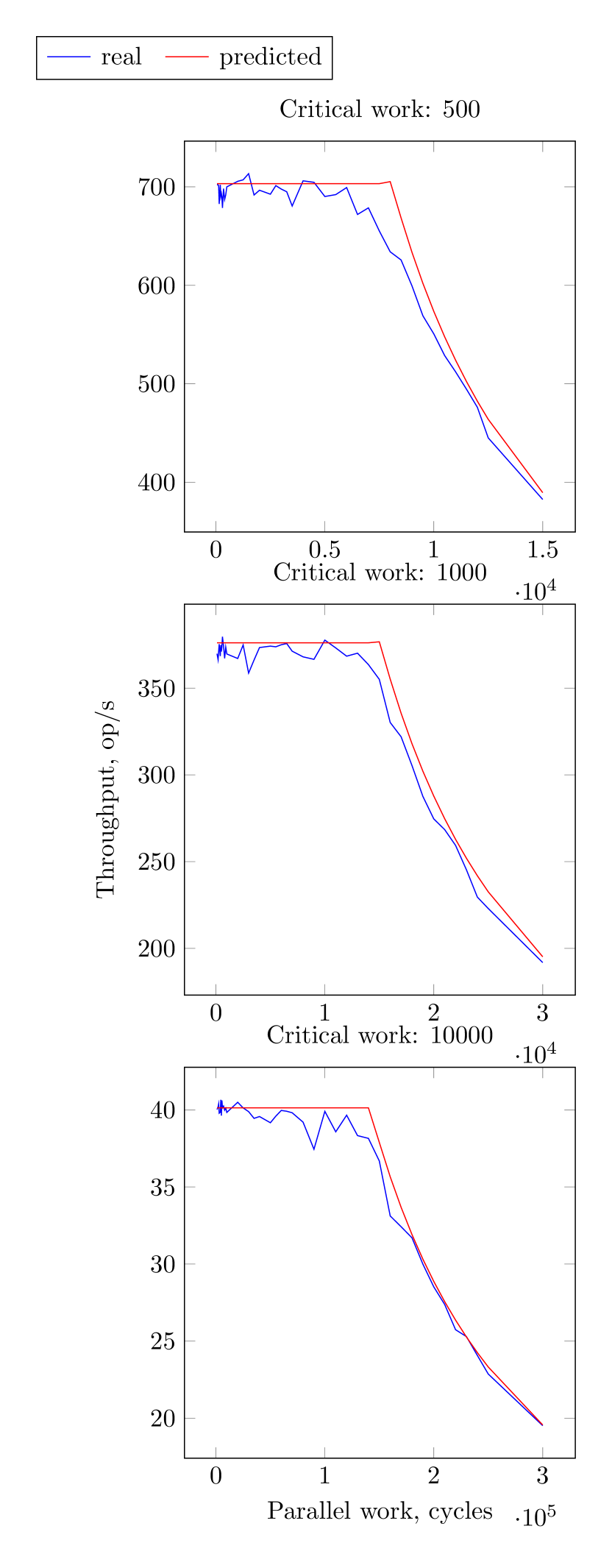
Figure 3. Throughput on $15$ processes for $C\in\{500,1000,10000\}$

⬇

1class Node:

2 bool locked // shared, atomic

3 Node next = null

4

5tail = null // shared, global

6myNode = null // per process

7

8operation():

9 myNode.next = null // $W$

10 myNode.locked = true // $W$

11 pred = swap(&tail, myNode) // $W$ or $X$

12 if pred != null:

13 pred.next = myNode // $W$

14 while myNode.locked: nop // $R_{I}$

15 // CS started

16 for i in 1..C: nop // $C$

17 // CS finished

18 if myNode.next == null: // $R_{I}$ or $R_{M}$

19 if tail.CAS(myNode,null): // $W$ or $X$

20 goto parallel

21 else:

22 while myNode.next == null: nop // $R_{I}$

23 //pass

24 myNode.next.locked = false // $W$

25 //Parallel section

26 parallel:

27 for i in 1..P: nop // $P$

Figure 4. The coarse-grained operation with inlined lock and unlock functions

Now the throughput can be expressed as: $\frac{\alpha}{C+2R_{I}+W}$ if $P+4\cdot W\leq(N-1)\cdot(C+2R_{I}+W)$, and $\frac{\alpha\cdot N}{P+C+R_{M}+4W}$ if $P+2\cdot W\geq(N-1)\cdot(C+2R_{I}+W)+R_{I}-R_{M}$.

To describe what is happening in between these two extremes, we can use linear approximation.

4. Experiments

The code of our benchmark is written in C++. We use an Intel Xeon Gold 6230 machine with 16 cores. Based on a single test run, we evaluate the constants as follows: $\alpha\approx 4.04\cdot 10^{5}$, $W\approx 15$, $R_{I}\approx 30$, and $R_{M}\approx 15$. In Figure 3, we depict our measurement results (in blue) and our analytical predictions (in red) for three values of $C\in\{500,1000,10000\}$ on $15$ processes. Here $x$ axis specifies the size of the parallel section and at the $y$ axis— the throughput. As one can see, our prediction matches the experimental results almost perfectly. The results of our experiments on an AMD machine are given in Appendix C.

5. Conclusion

In this short paper, we showed that in the model presented in (Aksenov et al., 2018) one can accurately predict the throughput of lock-based data structures not only when the lock is CLH, but also when the lock is MCS. Further, we want to close the gap by predicting the performance of data structures with the rest lock-types, such as spin locks, etc. Finally, we want to check whether in this model we can predict the throughput of lock-free data structures, such as Treiber’s stack.

Appendix A Analysis

A.1. The first case. Lock is unlocked.

We start with the first case. The corresponding schedule is presented on Figure 2(a). The first process performs two writes each with cost $W$ in Lines 9 and 10, a contended swap with cost $X$ in Line 11 while other processes perform two writes with cost $W$, a contended swap with cost $X$, and a write with cost $W$ in Line 13. Then, the first process performs: 1) the critical section with cost $C$; 2) a read from an invalid cache line with cost $R_{I}$ in Line 18 (on the first try, there is the second process waiting for the lock); 3) unlock the next process with cost $W$ in Line 24; 4) the parallel section of cost $P$; 5) two writes of cost $W$ in Lines 10 and 9; 6) a swap with null of cost $W$ in Line 11 since it is already uncontended; 7) the critical section with cost $C$; 8) a read from the exclusive cache line with cost $R_{M}$ in Line 18 since it has not been changed from Line 9; 9) a CAS of cost $W$ in Line 19; 10) the parallel section of cost $P$; 11) continue from the point 5) again.

The other processes do the similar thing. All other processes perform: 1) the invalid read of cost $R_{I}$ at Line 14 since there was the previous process waiting for the lock; 2) the critical section with cost $C$; 3) an invalid read of cost $R_{I}$ at Line 18 (please, note that process $n$ spends there only $R_{M}$, since for him the queue is empty); 4) unlock with cost $W$ in Line 24 or, for $n$-th process, make a successful CAS of cost $W$ in Line 19; 5) the parallel section of cost $P$; 6) continue from the point 5) for the first process.

Please, note that this was possible due to the fact that $R_{I}\geq W$, otherwise, the second process will not go to the point 6) for the first process and there will be a conflict on tail. Also, this schedule can happen only when the parallel section with two writes of the first process is bigger than the preliminary work of all other processes: $P+2W\geq(N-1)\cdot(2R_{I}+W+C)+R_{M}-R_{I}$. ($R_{M}$ happens for $n$-th process). And the throughput in that case becomes $\frac{\alpha N}{4W+R_{M}+C+P}$.

A.2. The second case. Lock is always taken.

We continue with the second case. The corresponding schedule is presented on Figure 2(b). The first process performs two writes each with cost $W$, a contended swap in Line 11 with cost $X$ while other processes perform two writes with cost $W$, a contended swap with cost $X$, and a write with cost $W$ in Line 13. Then, the first process performs: 1) the critical section with cost $C$; 2) a read from an invalid cache line of cost $R_{I}$ in Line 18 since the queue is not empty; 3) unlock the next process with cost $W$ in Line 24; 4) the parallel section of cost $P$; 5) two writes of cost $W$ each in Lines 10 and 9; 6) an uncontended swap of cost $W$ in Line 11; 7) adding the process to the queue with cost $W$ in Line 13; 8) wait until the process becomes unlocked with an invalid read with cost $R_{I}$ in Line 14; 9) continue from the point 1) again.

Any other process start at the point 8) and continue the program of the first process. This case is possible when $P+4W\leq(N-1)\cdot(2R_{I}+W+C)$ with the throughput of $\frac{\alpha}{2R_{I}+W+C}$.

Appendix B Experiments. Intel.

Results of more experiments on different critical section sizes from $\{500,1000,5000,10000,50000\}$ and the number of processes from $\{5,10,15\}$ can be seen on Figure 5.

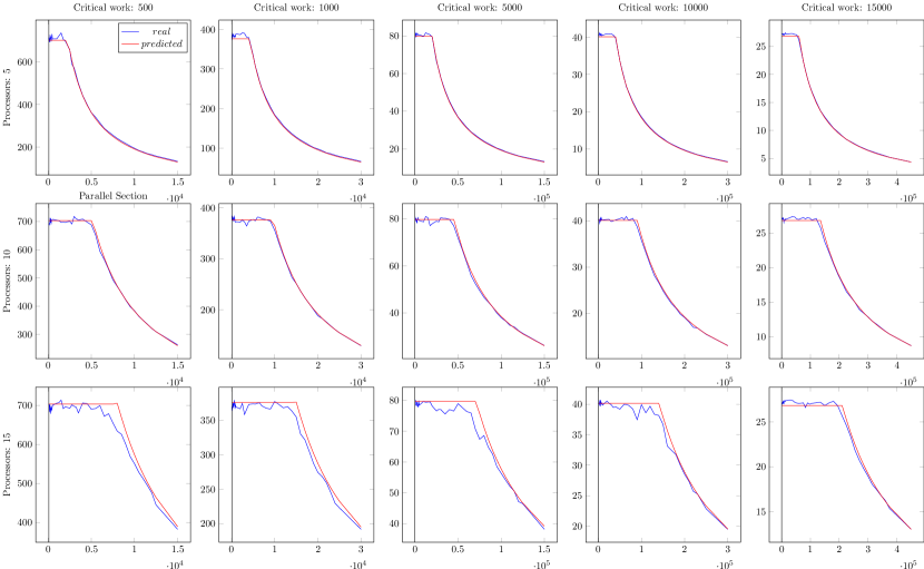
Figure 5. Throughput on $\{5,10,15\}$ processes for $C\in\{500,1000,5000,10000,50000\}$. Intel.

Appendix C Experiments. AMD.

We use a machine with one AMD Opteron 6378 with 16 cores. We estimate the constants once during the one chosen run as $\alpha\approx 1.24\cdot 10^{5}$, $W\approx 20$, $R_{I}\approx 35$, and $R_{M}\approx 15$. The plot 6 contains the real-life (blue) line and our expectation (red) line for five different values of critical section $C\in\{500,1000,5000,10000,50000\}$ on $\{5,10,15\}$ processes with the size of the parallel section at OX and throughput at OY axis. As one can see our prediction almost matches the experiment.

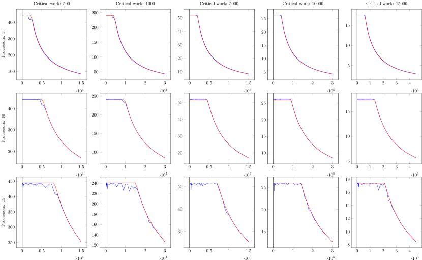
Figure 6. Throughput on $\{5,10,15\}$ processes for $C\in\{500,1000,5000,10000,50000\}$. AMD.

References

- (1)
- Aksenov et al. (2018) Vitaly Aksenov, Dan Alistarh, and Petr Kuznetsov. 2018. Brief Announcement: Performance Prediction for Coarse-Grained Locking. In Proceedings of the 2018 ACM Symposium on Principles of Distributed Computing, PODC 2018, Egham, United Kingdom, July 23-27, 2018. 411–413.
- Atalar et al. (2015) Aras Atalar, Paul Renaud-Goud, and Philippas Tsigas. 2015. Analyzing the Performance of Lock-Free Data Structures: A Conflict-Based Model. In Distributed Computing - 29th International Symposium, DISC 2015, Tokyo, Japan, October 7-9, 2015, Proceedings. 341–355.
- Atalar et al. (2016) Aras Atalar, Paul Renaud-Goud, and Philippas Tsigas. 2016. How Lock-free Data Structures Perform in Dynamic Environments: Models and Analyses. In 20th International Conference on Principles of Distributed Systems, OPODIS 2016, December 13-16, 2016, Madrid, Spain. 23:1–23:17.
- Atalar et al. (2018) Aras Atalar, Paul Renaud-Goud, and Philippas Tsigas. 2018. Lock-Free Search Data Structures: Throughput Modeling with Poisson Processes. In 22nd International Conference on Principles of Distributed Systems (OPODIS 2018). Schloss Dagstuhl-Leibniz-Zentrum fuer Informatik.
- Craig (1993) Travis Craig. 1993. Building FIFO and priorityqueuing spin locks from atomic swap. Technical Report. ftp://ftp.cs.washington.edu/tr/1993/02/UW-CSE-93-02-02.pdf
- David et al. (2013) Tudor David, Rachid Guerraoui, and Vasileios Trigonakis. 2013. Everything you always wanted to know about synchronization but were afraid to ask. In Proceedings of the Twenty-Fourth ACM Symposium on Operating Systems Principles. ACM, 33–48.
- JáJá (1992) Joseph JáJá. 1992. An introduction to parallel algorithms. Vol. 17. Addison-Wesley Reading.
- Mellor-Crummey and Scott (1991) John M Mellor-Crummey and Michael L Scott. 1991. Algorithms for scalable synchronization on shared-memory multiprocessors. ACM Transactions on Computer Systems (TOCS) 9, 1 (1991), 21–65.
- Papamarcos and Patel (1984) Mark S Papamarcos and Janak H Patel. 1984. A low-overhead coherence solution for multiprocessors with private cache memories. In ACM SIGARCH Computer Architecture News, Vol. 12. ACM, 348–354.