Satellite galaxy abundance dependency on cosmology in Magneticum simulations

Abstract

Context. Observational studies as mass-calibrations of galaxy clusters often use mass-richness relations to interpret galaxy number counts.

Aims. To study the impact of parametrising the richness-mass relation with cosmological parameters in mock mass-calibrations, and to understand if this modelling could be inferred by dark-matter only simulations.

Methods. We build a Gaussian Process Regression emulator of satellite abundance normalisation and log-slope based on cosmological parameters $\Omega_{m},\Omega_{b},\sigma_{8},h_{0}$ and redshift $z.$ We train our emulator using Magneticum hydrodynamic simulations that span different cosmologies for a given set of feedback scheme paremeters.

Results. We find that the normalisation depends on cosmological parameters, even if weakly, especially on $\Omega_{m},$ $\Omega_{b},$ and that their inclusion in mock-observations increase their constraining power of $10\%.$ On the other hand the log-slope is $\approx 1$ on every setup, and the emulator does not predict it with significant accuracy. We also show that satellite abundance cosmology dependency differs between full-physics simulations, dark-matter only, and non-radiative simulations.

Conclusions. Mass-calibration studies would benefit by modelling the mass-richness relations with cosmological parameters, especially if this dependency is calibrated from full-physics simulations.

1 Introduction

Properties of galaxies within galaxy clusters (GCs) are connected to the properties of their underlying halo. This relationship, defined as the Galaxy-Halo (G-H) connection (see Wechsler & Tinker, 2018, for a complete review on the topic and its applications) provides a powerful framework to test galaxy formation models (Reid et al., 2014; Coupon et al., 2015; Rodríguez-Puebla et al., 2017), to constrain cosmological parameters (Leauthaud et al., 2017), and as a proxy to calibrate halo masses (Zenteno et al., 2016).

One key topic in the G-H connection is the HOD (see Kravtsov et al., 2004, for a pioneering study on this topic), namely the conditional probability distribution $P(N|M)$ that a halo of mass $M$ has a galaxy abundance $N.$ In the context of HOD, galaxy counting is separated into central $N_{c}$ and satellite $N_{s}$ abundances so that:

$$N\equiv N_{c}+N_{s}.$$ (1)

In fact, central and satellite galaxies belong to two different populations as they experience different processes (Guzik & Seljak, 2002) as shown by both observations (Skibba, 2009) and numerical simulations (Wang et al., 2018): the satellite galaxy abundance distribution $P(N_{s}|M)$ (i.e. the satellite HOD) is typically modelled with a Poisson distribution at each mass bin (Kravtsov et al., 2004) and its average value should increase with halo mass; while the number of central galaxies $N_{c}$ tends to unity asymptotically with respect to the galaxy mass selection threshold. The average $Ns-M$ relation is typically modelled with a power law at high halo masses,

$$\langle N_{\texttt{s}}\rangle_{M}\propto M^{\beta}.$$ (2)

Subhalo population is affected by the host halo accretion history (Giocoli et al., 2008) and HOD normalisation has a mild evolution with redshift as noted in Kravtsov et al. (2004). The log-slope $\beta$ plays a key role in galaxy formation efficiency and it is not yet well constrained.

Constraining the HOD is crucial for interpreting many observational studies (see e.g. Ross et al., 2010), and there are efforts to model HOD using additional halo properties besides mass: assembly bias (Hearin et al., 2016), the environment (Voivodic & Barreira, 2020; Hadzhiyska et al., 2021b), a combination of them (Yuan et al., 2021), concentration (Avila et al., 2020), velocity dispersion (Hadzhiyska et al., 2021a). However, most observational studies deal with a catalogue that have poor or no knowledge about their halo accretion histories (see e.g. Costanzi et al., 2019), part of this work is devoted in understanding if the dependency of satellite abundance from cosmological parameters can improve mass-calibration studies.

There are works in the literature that study how galaxy populations are affected by variation of cosmological parameters (see e.g. van den Bosch et al., 2005; Wang et al., 2008). However, since baryons are known to play a role inside galaxy clusters (Despali & Vegetti, 2017; Castro et al., 2021), in this work we will show that satellite abundance of DMO and full-physics (FP) simulations are affected differently from changes in cosmological parameters.

We will use Magneticum suite of hydrodynamic simulations (Biffi et al., 2013; Saro et al., 2014; Steinborn et al., 2015; Teklu et al., 2015; Dolag et al., 2015, 2016; Steinborn et al., 2016; Bocquet et al., 2016; Remus et al., 2017; Ragagnin et al., 2019). Here we employ a set of $15$ runs with same initial conditions and run on different cosmological parameters (Singh et al., 2020; Ragagnin et al., 2021) and were run with the same feedback scheme parameters.

The paper is structured as follows: in Sect. 2, we describe in detail the numerical set up of the simulations used in this work. In Sec. 3, we justify the need of studying HOD cosmology dependency with FP simulations instead of DMO simulations. In Sect. 4, we fit the satellite abundance for all our simulations and snapshots, build an emulator, and test it. We devote Sect. 5 to studying the effect of employing an emulator in mock observations. We draw our conclusions in Sect. 6.

2 Magneticum Simulations

Table 1: Magneticum simulation specifications used in this work: the Box0/mr, Box1a/mr, Box2/hr, and Box4/uhr. Columns from left to right present, the name, the cosmology (see Table 2), the box size in comoving $\mathrm{Mpc}/h,$ dark matter and initial gas particle masses $m_{\mathrm{D}M},m_{\mathrm{g}as},$ and gravitational softening for dark matter, gas and stars $\epsilon_{\mathrm{D}M}$, $\epsilon_{\mathrm{g}as}$, $\epsilon_{\mathrm{s}tars}$.

Name	Cosmologies	Box size	$m_{DM}$	$m_{gas}$	$\epsilon_{DM}$	$\epsilon_{gas}$	$\epsilon_{stars}$
		$[a\mathrm{Mpc}/h]$	$\Bigl{[}M_{\odot}/h\frac{\displaystyle\Omega_{m}}{\displaystyle\Omega_{m,WMAP7}}\Bigr{]}$	$\Bigl{[}M_{\odot}/h\frac{\displaystyle\Omega_{b}}{\displaystyle\Omega_{b,WMAP7}}\Bigr{]}$	$[a\mathrm{kpc}/h]$	$[a\mathrm{kpc}/h]$	$[a\mathrm{kpc}/h]$
Box0/mr	C8	2688	$1.3\cdot 10^{10}$	$2.6\cdot 10^{9}$	10	10	5
Box1a/mr	C1-15	896	”	”	”	”	”
Box2/hr	C8	352	$6.9\cdot 10^{8}$	$1.4\cdot 10^{8}$	3.75	3.75	2
Box4/uhr	C8	48	$3.6\cdot 10^{7}$	$7.3\cdot 10^{6}$	1.4	$1.4$	$0.7$

Table 2: List of Magneticum cosmologies for the Box1a/mr C1–C15 simulations. Starred row (C8^⋆) represents the original runs on WMAP7 cosmological parameters. Columns from left to right present, the name, and cosmological parameters $\Omega_{m},\Omega_{b},\sigma_{8},h_{0}$, respectively.

Name	$\Omega_{m}$	$\Omega_{b}$	$\sigma_{8}$	$h_{0}$
C1	0.153	0.0408	0.614	0.666
C2	0.189	0.0455	0.697	0.703
C3	0.200	0.0415	0.850	0.730
C4	0.204	0.0437	0.739	0.689
C5	0.222	0.0421	0.793	0.676
C6	0.232	0.0413	0.687	0.670
C7	0.268	0.0449	0.721	0.699
C8⋆	0.272	0.0456	0.809	0.704
C9	0.301	0.0460	0.824	0.707
C10	0.304	0.0504	0.886	0.740
C11	0.342	0.0462	0.834	0.708
C12	0.363	0.0490	0.884	0.729
C13	0.400	0.0485	0.650	0.675
C14	0.406	0.0466	0.867	0.712
C15	0.428	0.0492	0.830	0.732

Magneticum simulations are based on the N-body code P-Gadget3, which is an improved version of P-Gadget2 (Springel et al., 2005b; Springel, 2005; Boylan-Kolchin et al., 2009), with a space-filling curve aware neighbour search (Ragagnin et al., 2016), and an improved Smoothed Particle Hydrodynamics (SPH) solver (Beck et al., 2016). These simulations include a treatment of radiative cooling, heating, ultraviolet (UV) background, star formation and stellar feedback processes as in Springel et al. (2005a) connected to a detailed chemical evolution and enrichment model as in Tornatore et al. (2007), which follows 11 chemical elements (H, He, C, N, O, Ne, Mg, Si, S, Ca, Fe) with the aid of CLOUDY photo-ionisation code (Ferland et al., 1998). Fabjan et al. (2010); Hirschmann et al. (2014) describe prescriptions for black hole growth and for feedback from AGNs.

Haloes together with their member galaxies are identified using respectively, the FoF halo finder (Davis et al., 1985) and an improved version of the subhalo finder SUBFIND (Springel et al., 2001), that takes into account the presence of baryons (Dolag et al., 2009).

In this work, we mainly focus on a set of $15$ simulations labelled Box1a/mr C1–C15 simulations. They span a range of total matter fraction $0.153<\Omega_{m}<0.428,$ baryon fraction $0.0408<\Omega_{b}<0.0504,$ power spectrum normalisation $0.650<\sigma_{8}<0.886,$ and reduced Hubble constant $0.670<h_{0}<0.732,$ as presented in Tables 1 and 2, and are centered around the one of C8, that has WMAP7 cosmological parameters. For each simulation we study the haloes at a time slice with redshifts $z=0.00,\ 0.14,\ 0.29,\ 0.47.$

In order to study resolution and mass-range of our emulator, we will use three additional Magneticum simulations, all with the same WMAP7 cosmology as C8: we use a high-resolution (HR) simulation Box2/hr (Hirschmann et al., 2014); we use a ultra-high resolution simulation Box4/uhr (Teklu et al., 2015) to study the emulator mass range validity on low-mass haloes; and a large-volume MR simulation (Box0/mr, Bocquet et al., 2016) in order to validate our satellite HOD results up to the most massive galaxy clusters of the Universe. Note that the phases of the initial conditions of these three boxes are different.

In this works, all masses and radius are expressed in physical units (unless in Table 1 where the units has been chosen differently for the sake of conciseness), thus they are not implicitly divided by $(1+z)$ or $h_{0}$ as other works on simulations.

3 DMO vs. FP simulations

In this section we demonstrate the need of employing FP simulations (as opposed to DMO ones) in studies that aim to model the mass-richness relation as a function of cosmology. In particular we will show that FP $N_{s}$ cosmology dependency differs from adiabatic runs (i.e. runs with no cooling and star formation, hereafter norad) or DMO simulations.

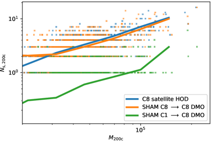
Figure 1: Satellite count $N_{\texttt{s},200c}$ $vs.$ halo mass $M_{\texttt{2}00c},$ respectively for C8 (blue coloured data), SHAM C8 DMO (orange coloured data), SHAM C8 DMO from C1 (green coloured data). Each data point represents a halo, solid lines represent the mean abundance per mass bin.

To this end, we first show that satellite HOD cannot be recovered in a DMO simulation using Subhalo Abundance Matching (SHAM) technique from a FP simulation that was run on a different cosmology. For this purpose we perform mock SHAMs (with a stellar mass cut $M_{\star}>2\cdot 10^{11}M_{\odot}$) to C8 DMO both from its FP counterpart C8, and from C1. Figure 1 shows the resulting $N_{s}-M$ relations for these setups, and as expected, we find that SHAM from C8 to C8 DMO does match the original C8 FP average values. Additionally, we see that using C1 to perform SHAM on C8 DMO leads to a too low $N_{s}$.

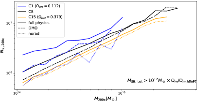
Figure 2: Satellite count $N_{\texttt{s},200c}$ $vs.$ halo mass $M_{\texttt{2}00c}$ for Box1a/mr C1 (blue higher lower lines), C8 (black intermediate lines) and C15 (orange lower lines) simulations, their non-radiative (dotted lines, abbreviated with norad) counterpart, and their DMO counterparts (dashed lines). For galaxy masses $M_{\texttt{S}H,tot}$ greater than $10^{12}{\rm M}_{\odot}\times\Omega_{m}/\Omega_{m,{\textrm{W}MAP7}}.$

The reason of this mismatch lies in the fact that cosmological parameters have a different impact on sub-haloes evolution of DMO runs and on galaxy evolution of FP runs. To prove this statement, in Figure 2 we compute $\langle N_{s}\rangle_{M}$ for two cosmologies of which we have the norad counterparts, Box1a/mr C1 and C15, and for two cosmologies of which we have the DMO counterpart, C8 and C1. Since DMO and norad simulations have no stars, here we count galaxies based on their total mass $M_{\rm GAL,tot}>10^{12}{\rm M}_{\odot},$ re-scaled by $\Omega_{m}/\Omega_{m,\rm WMAP7}.$

First of all, we note that C8 DMO $Ns-M$ relation is systematically steeper than the respective FP run, thus these kind of relations are strongly affected by the presence of baryons. Additionally, we can see that C15 and its norad counterpart have almost the same satellite count, while C1 and its norad counterpart differ of more than a factor of two, thus the effect of baryons on the $N_{s}-M$ relation does depend on cosmological parameters. These two experiments shows that studying HOD dependency on non-FP simulations would have produced a different cosmology dependency than the one found in this work.

4 Satellite abundance emulator

In this section we will train an emulator in order to extrapolate the mass-richness relation for some arbitrary cosmological parameters (that are within the range of the parameters of our simulations). We will use this emulator in the next Section, where we will estimate the benefit of using it in mock mass-calibration studies. To this end, we first searched for a stellar-mass cut that makes the richness of Box1a/mr C8 to converge with its high-resolution counter-part Box2b/hr (see Appendix A for more details), and found that if we limit ourselves to galaxies with $M_{\star}>2\cdot 10^{11}{\rm M}_{\odot},$ then the two simulations have the same mass-richness relations. This relatively-high stellar-mass cut could introduce a bias in the satellite population, however this mass-range should still be enough to constrain the normalisation and log-slope of a power-law modelling.

We found that Box2/hr satellite HOD offset between its fiducial stellar mass cut ($10^{10}{\rm M}_{\odot}$) and the C8 stellar mass cut ($2\cdot 10^{11}{\rm M}_{\odot}$) is

$$\frac{\displaystyle N_{\texttt{s}}\left(M_{\star}>10^{10}{\rm M}_{\odot}\right)}{\displaystyle N_{\texttt{s}}\left(M_{\star}>2\cdot 10^{11}{\rm M}_{\odot}\right)}\approx 31.$$ (3)

We consider this ratio useful to compare emulated satellite abundance values (based on C1–C15 MR simulations) predictions together with HR simulations in literature with a cut $M_{\star}>10^{10}{\rm M}_{\odot}$.

To estimate the satellite count and compare it consistently between different cosmologies, one must choose a minimum stellar mass cut for each set of cosmological parameters. Following Anbajagane et al. (2020) we decided to re-scale the satellite stellar mass cut with $M_{\star}>2\cdot 10^{11}{\rm M}_{\odot}\cdot f_{b}/f_{b,\texttt{WMAP7}}.$ In order to keep the satellite HOD in the power-law regime, we imposed a halo mass cut so that a given mass bin has at least one halo with $8$ satellites. After this cut, we found that two setups ended with only few haloes above the mass-cut, so we removed them from further analyses.

4.1 $N_{\texttt{s}}-M$ relation fit

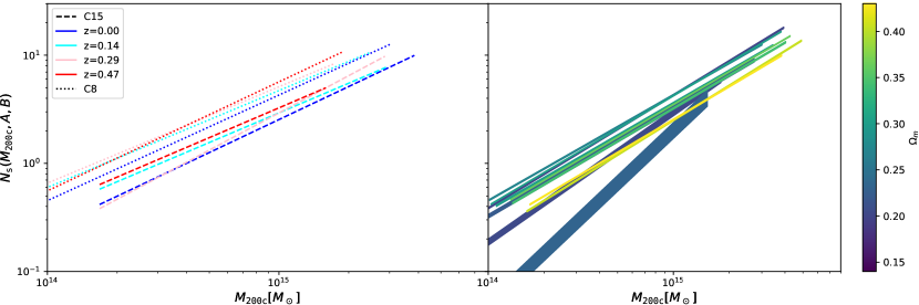
Figure 3: Average satellite count within $R_{\mathrm{200c}}$ $vs.$ halo mass for different simulations and redshifts as resulting from maximising Likelihood in Eq. (5). Left panel: relation for simulations Box1a/mr C8 (dashed lines) and C15(dotted lines) at 3 different redshifts (the redder the redshifted). Right panel: each line represents a simulation at $z=0,$ color coded with green with increasing $\Omega_{m};$ line tickness covers the gaussian scatter (poissonian scatter is omitted).

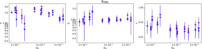
Figure 4: Fit parameters of Eqs. (5) and (4) for $N_{\texttt{s,200c}}.$ From left to right, parameters $A,B,\sigma$ as a function of $\Omega_{m}$ and colour-coded by $1+z$ (the redder, the higher the red-shift). Vertical error bars corresponds to the uncertainty given from the Likelihood posterior in Eq. (5).

We model the average satellite abundance as a power law of halo mass as in Eq. (2), with a normalisation $A$ and log-slope $\beta$ as follows

$$\langle N_{s}\rangle_{M}=N_{\texttt{s}}\left(M,A,\beta\right)=A\cdot\left(\frac{M}{M_{p}}\right)^{\beta},$$ (4)

where we use $M_{p}=5\times 10^{14}M_{\odot}$ as pivot mass, because it approximates the median mass of the haloes selected at $z=0$ in the reference cosmology $C8.$

We fit $A$ and $\beta$ parameters by maximising a likelihood $\mathcal{L}$ that models satellite HOD as the convolution of a Poisson and a positive-value Gaussian distribution, with fractional scatter $\sigma$ on the average satellite abundance. This kind of modelling has been used in the mass-calibration studies as Costanzi et al. (2019) and Abbott et al. (2020) where the positive-values Gaussian scatter accounts for different accretion histories. The likelihood results as follows:

$$\mathcal{L}\left(A,\beta,\sigma\right)=\prod_{i}{\frac{\int_{0}{\mathcal{P}\left(N_{\texttt{s},i}|n\right)\mathcal{N}\left(n\big{|}N_{\texttt{s}}\left(M_{i},A,\beta\right),\sigma N_{\texttt{s}}\left(M_{i},A,\beta\right)\right)}\mathrm{d}n}{\int_{0}{\mathcal{N}\left(n\big{|}N_{\texttt{s}}\left(M_{i},A,\beta\right),\sigma N_{\texttt{s}}\left(M_{i},A,\beta\right)\right)}}}\,,$$ (5)

where $i$ runs over all haloes that we selected in a snapshot.

We maximised the likelihood in Eq. (5) for all simulations separately and Figure 3 shows the power law fit for C8 and C15 at all available redshift (left panel) and for all simulations at $z=0$ (right panel). The shaded area corresponds to the Gaussian scatter $\sigma$, showing that average satellite abundances differ on different cosmologies. We can qualitatively see that different cosmologies and redshifts lead to values of $\beta$ that are close to $1$ and a normalisation that can vary up to a factor of two. See Appendix B for more details on the fit values.

One may argue that the dependency from cosmological parameters on $N_{s}$ is rooted on the fact that $N_{s}$ depends on halo concentration and the halo concentration depends on cosmology. However, even if concentration and assembly bias play a role in the satellite count, it cannot account completely for the dependency between cosmological parameters shown in Fig. 3. In fact, Box1a/mr C13 simulation has an outstandingly low number of satellites (it has no halo with $N_{s}\geq 8$ and in fact it is not included in the emulator), while it has not a particularly high concentration-mass normalisation (see Fig. 2 in Ragagnin et al., 2021). In Figure 4, we summarise the parameters $A,\beta,$ and $\sigma$ found by maximising Eq. (5) for $\Delta_{\texttt{200c}}$, where we can see a mild redshift evolution of $A$ and $\beta$ as found in Kravtsov et al. (2004). An increase of $N_{s}$ with redshift could be expected since at high redshift we are selecting more and more young clusters (the mass-cut does not change with redshift), and young clusters are known to be richer  (see Bose et al., 2019).

4.2 The gaussian process regression emulator

In order to model the HOD as a function of cosmological parameters and redshift, we will build an emulator based on Gaussian process regression (GPR) with the aim of predicting $A,\beta,$ and $\sigma.$ Our main motivation is that these parameters do not follow simple functional forms, as for instance a power law, as can be seen in Fig. 4.

For this purpose we train the GPR model on an array of $A_{i},\beta_{i},$ and $\sigma_{i}$ residuals with respect to a power-law fit on cosmological parameters (where $i$ runs on all setup). We present fit posteriors in Appendix C, and here below we report the results and errros from the fit:

$$\begin{split}\textrm{ln}\left(A_{\texttt{2}00c}\right)=&0.551_{-0.041}^{0.045}-1.304_{-0.224}^{0.246}\textrm{ln}\Bigl{(}\frac{\Omega_{m}}{\Omega_{m,p}}\Bigr{)}+3.008_{-1.104}^{1.093}\textrm{ln}\Bigl{(}\frac{\Omega_{b}}{\Omega_{b,p}}\Bigr{)}\\ &+4.037_{-0.823}^{0.610}\textrm{ln}\Bigl{(}\frac{\sigma_{8}}{\sigma_{8,p}}\Bigr{)}-0.803_{-1.982}^{1.974}\textrm{ln}\Bigl{(}\frac{h_{0}}{h_{0,p}}\Bigr{)}\end{split}$$ (6)

$$\begin{split}&-0.878_{-0.323}^{0.267}\textrm{ln}\Bigl{(}\frac{a}{a_{p}}\Bigr{)}\pm 0.2\\ \textrm{ln}\left(\beta_{\texttt{2}00c}\right)=&0.043_{-0.030}^{0.028}+0.288_{-0.185}^{0.177}\textrm{ln}\Bigl{(}\frac{\Omega_{m}}{\Omega_{m,p}}\Bigr{)}-0.931_{-0.826}^{0.850}\textrm{ln}\Bigl{(}\frac{\Omega_{b}}{\Omega_{b,p}}\Bigr{)}\\ &-1.056_{-0.664}^{0.690}\textrm{ln}\Bigl{(}\frac{\sigma_{8}}{\sigma_{8,p}}\Bigr{)}-0.775_{-1.586}^{1.590}\textrm{ln}\Bigl{(}\frac{h_{0}}{h_{0,p}}\Bigr{)}\\ &+0.080_{-0.155}^{0.162}\textrm{ln}\Bigl{(}\frac{a}{a_{p}}\Bigr{)}\pm 0.1,\end{split}$$ (7)

where pivot cosmology parameters are set to C8 values and pivot scale factor is $a=0.87.$

We trained our emulator on log-scaled values, as follows:

$$\begin{cases}X_{i}=\Bigl{[}\par\textrm{ln}\Bigl{(}\dfrac{\Omega_{m,i}}{\Omega_{m,p}}\Bigr{)},\textrm{ln}\Bigl{(}\dfrac{\Omega_{b,i}}{\Omega_{b,p}}\Bigr{)},\textrm{ln}\Bigl{(}\dfrac{\sigma_{8,i}}{\sigma_{8,p}}\Bigr{)},\textrm{ln}\Bigl{(}\dfrac{h_{0,i}}{h_{0,p}}\Bigr{)},\textrm{ln}\Bigl{(}\dfrac{1+z_{p}}{1+z_{i}}\Bigr{)}\Bigr{]}\\ \\ y_{i}=\Bigl{[}\textrm{ln}\Bigl{(}\dfrac{A_{i}}{A_{\Delta}}\Bigr{)},\textrm{ln}\Bigl{(}\dfrac{\beta_{i}}{\beta_{\Delta}}\Bigr{)},\textrm{ln}\Bigl{(}\dfrac{\sigma_{i}}{\sigma_{\Delta}}\Bigr{)}\Bigr{]}\ ,\end{cases}$$ (8)

where $X=\left\{X_{i}\right\}$ is the input data; $y=\left\{y_{i}\right\}$ the output data; $i$ runs over all data points (i.e. all selected snapshots) for which we maximised Likelihood in Eq. (5), and $A_{\Delta},\beta_{\Delta},$ and $\sigma_{\Delta}$ are a function of cosmology and, as pivot values, we used the same as in Eq. (6) and Eq. (7).

Concerning the GPR model, we modelled our kernel $K$ as a constant $K_{0},$ times a gaussian Radial-basis function (RBF) kernel with length scale $l$:

$$K(\mathbf{x_{1}},\mathbf{x_{2}})=K_{0}\times\mathrm{exp}\left(-\frac{\left\lVert\mathbf{x_{1}}-\mathbf{x_{2}}\right\lVert^{2}}{2l^{2}}\right),$$ (9)

where the norm $\left\lVert\dotsc\right\rVert$ is the euclidean distance.

We maximised the log marginal likelihood as proposed in Eq. 2.30 in Rasmussen & Williams (2005) and let parameters $K_{0}$ and $l$ to vary in the maximisation.

Hereafter we define the Emulator predictions as $A^{\textrm{Emu}},$ $\beta^{\textrm{Emu}},$ which themselves depends on a cosmology and scale factor $(\Omega_{m},\Omega_{b},\sigma_{8},h_{0},a).$ We define the emulated average number of satellites $N_{\mathrm{s,Emu}}$ as

$$N_{\textrm{s,Emu}}=A_{\textrm{Emu}}\times\left(\frac{M}{M_{p}}\right)^{{\beta_{\textrm{Emu}}}},$$ (10)

where $A_{\textrm{Emu}},$ and $\beta_{\textrm{Emu}}$ are predicted by our emulator an depend on cosmology and redshift.

4.3 Emulator error estimate

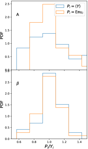
Figure 5: PDF of residuals for predictor $P_{i}=\textrm{Emu}_{i}$ and the residual based on predictions from the average values ($P_{i}=\langle Y\rangle$), with respect to the missing data point $y_{i}.$ Data is computed on overdensity $\Delta_{\mathrm{200c}}.$ Upper row show PDF for $y_{i}=A_{i},$ lower row show PDF for $y_{i}=\beta_{i}.$ The scatter obtained with the emulator is significantly smaller than the residuals on the averages

To estimate the precision of our emulator we use the same technique as used by Bocquet et al. (2020): for each data vector available $(X_{i},y_{i})$, we (i) build a predictor trained on the complete data-set but that point (i.e. $[X,Y]_{i}=[\{X\}\setminus X_{i},\{Y\}\setminus y_{i}]$), hereafter $O_{{\tt Emu},i}$ and (ii) for each predictor we compute its relative error in predicting the un-trained value $y_{i}.$

To contextualise the relative error of the emulator, we will compare it with the relative error obtained by predicting $y_{i}$ using only the average of all values (thus ignoring any cosmology dependency).

As we can see in Figure 5, the residual PDF of the $A$ from the emulator emulators (top panel, orange steps) is much more peaked around $1$ respect to the PDF from the predictor based on the averages (blue steps). This implies that the emulator is effective in predicting mass-richness normalisation $A$. On the other hand there is no significant gains in recovering the log-slope $\beta.$

The residuals distribution of the emulator within $\Delta_{\mathrm{200c}}$ corresponds to a precision of $\approx 10-20\%,$ and the average of the GPR error estimations in the missing points is of the same order of magnitude, thus the emulator is capable of correctly predicting its own uncertainty.

4.4 Mass range

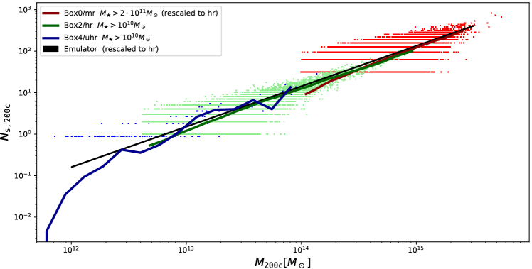
Figure 6: Satellite count $N_{\texttt{s},200c}$ $vs.$ halo mass $M_{\texttt{2}00c}$ for three Magneticum simulations, Box4/uhr (blue coloured), Box2/hr (green coloured), and Box0/mr (red colour) to account for resolution effects. Data points represents single haloes, coloured lines represents average values per mass bin. Black line is emulator prediction. Emulator and Box0/mr data are re-scaled with Eq. (3).

In this subsection we test the mass range validity of our satellite HOD across various orders of magnitude in order to identify the halo mass range of it.

Figure 6 shows that the same power law satellite abundance holds from the most massive galaxy clusters $M_{200c}\approx 6\cdot 10^{15}{\rm M}_{\odot}$ down to haloes of $M_{200c}\approx 5\cdot 10^{13}{\rm M}_{\odot}.$ At that mass there starts the low-mass drop of $M_{\star}>10^{10}{\rm M}_{\odot}$ cut, which is particularly visible in the Box4/uhr regime haloes. Both Box0/mr and C8 satellite abundances are re-scaled using in Eq. (3). The match between mass-richness relations from our emulator and various Magneticum boxes (some of which are rescaled using Equation 3), shows that Equation (3) is consistent between resolutions and that our relatively high stellar-mass cut is enough to constrain the normalisation and log-slope of the mass-richness relation.

4.5 Comparison with numerical studies

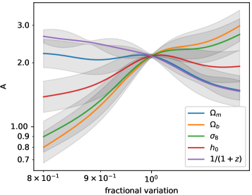
Figure 7: Variation of $N_{\mathrm{s,200c}}$ emulator $A$, $\beta$ and $\sigma$ as a function of fractional variation of cosmological parameters $\Omega_{m},\Omega_{b},\sigma_{8},h_{0}$ and scale factor. Shaded areas show $1$ standard deviation provided by the Gaussian Process error estimation.

We now investigate the effect of each cosmological parameter on the $N_{s}-M$ relation. Figure 7 shows the parameters $A_{\tt Emu},B_{\tt Emu}$ variation from WMAP7 cosmology values, as a function of fractional variation of each cosmological parameter $\Omega_{m},\Omega_{b},\sigma_{8},h_{0},$ and $a$ separately.

The normalisation decreases with scale factor, which is in agreement with the fact that BAHAMAS (that runs at $z=0.1$) has a higher normalisation than Magneticum (Anbajagane et al., 2020), yet it has very similar cosmological parameters. Note that this manuscript do not aim to predict HODs of the other simulation suites, rather, we show that their variation is comparable with the one predicted by changing cosmological parameters alone on fixed-feedback simulations. In Appendix D we compare in detail the mass-richness relation of our emulator and the one of other hydrodynamic simulations in the literature.

5 Impact on mock observations

In this section we test the cosmology-dependence of the HOD on mock catalogues, in order to estimate the impact of such dependence on the cosmological parameter constraints. To this purpose, we consider the richness, a weighted sum of the galaxy members, often used as mass proxy in photometric cluster surveys. We recast Eq. (4) in terms of a richness-mass relation:

$$\langle\lambda\rangle_{M}=A_{\lambda}\cdot\left(\frac{M}{M_{p}}\right)^{\beta_{\lambda}},$$ (11)

with $A_{\lambda}=A_{0}\cdot A_{\rm emu}=72.4\pm 0.7$ and $\beta_{\lambda}=\beta_{0}\cdot\beta_{\rm emu}=0.935\pm 0.038$ (from table IV of Costanzi et al., 2021). Here, $A_{\rm emu}$ and $\beta_{\rm emu}$ are the predictions of the emulator and contain the dependence on cosmology, while $A_{0}$ and $\beta_{0}$ represent the cosmology-independent part of the total parameters.

To perform the analysis, we extract a catalogue of halo masses corresponding to the C8 simulation at redshift $z=0$, following the Despali et al. (2016) analytical mass function. This step ensures to have a proper description of the mass function, in order to obtain an unbiased estimation of parameters. We obtain a catalogue with $\sim 2.8\cdot 10^{5}$ objects, with virial masses above $M_{\mathrm{vir}}>10^{13}{\rm M}_{\odot}$, to which we assign richness by applying Eq. (11), plus a Poisson scatter. To ease the analysis, we neglect the intrinsic scatter of the HOD, which is subdominant with respect the Poisson one. In the end, we compute the number counts by considering 5 richness bins, between $\lambda=30-300$, where the sample is complete in mass.

Then, we maximise a Gaussian likelihood

$$\mathcal{L}(x\,|\,\mu,\,C)=\frac{\displaystyle\exp{\left\{-\frac{1}{2}(\mathbf{x}-\boldsymbol{\mu})^{T}C^{-1}(\mathbf{x}-\boldsymbol{\mu})\right\}}}{\displaystyle\sqrt{2\pi\det C}}\,,$$ (12)

where $\mathbf{x}$ is the mock ”observed” number count and $\boldsymbol{\mu}$ is a MCMC test one, and $C$ is the covariance matrix, computed following the analytical model of Hu & Kravtsov (2003). Since in this test we only aim to give an estimation of the impact of the cosmology-dependent HOD, we run a simplified Monte Carlo Markov Chain (MCMC) process with only two free cosmological parameters, $\Omega_{\rm m}$ and $\log_{10}A_{s}$ (and thus $\sigma_{8}\,$), neglecting the dependence of the HOD on $\Omega_{\rm b}$ and $h_{0}$, and neglecting the redshift dependence.

Following the approach of Singh et al. (2020), we compare three different cases:

1. no cosmo case: we ignore the cosmology dependence of the HOD, so that $A_{\lambda}=A_{0}$ and $\beta_{\lambda}=\beta_{0}$. We assume flat uninformative priors both on $\Omega_{\rm m}\,$and $\log_{10}A_{\rm s}\,$and on $A_{\lambda}$ and $\beta_{\lambda}$;

2. cosmo case: we assume flat uninformative priors on $\Omega_{\rm m}\,$, $\log_{10}A_{\rm s}\,$, $A_{0}$ and $\beta_{0}$, plus Gaussian priors on $A_{\lambda}$ and $\beta_{\lambda}$, respectively given by $\mathcal{N}(72.4,7.0)$ and $\mathcal{N}(0.935,0.038)$. The cosmology-dependent parameters $A_{\rm emu}$ and $\beta_{\rm emu}$ are computed by the emulator at each step of the MCMC process, and, to take into account the emulator inaccuracy, we randomly extract a value from a Gaussian distribution with center in the emulator prediction and amplitude equal to $\sigma_{\log A_{\rm emu}}=0.06$ and $\sigma_{\log\beta_{\rm emu}}=0.09$;

3. cosmo + WL case: we add the weak lensing (WL) cosmological dependence which affects the mass calibration in the real observations, to figure out whether the combination of the cosmology-dependent HOD with other cosmological probes could improve the parameter constraints. We model such dependence by modifying the prior on $A_{\lambda}$, which becomes a Gaussian prior with the same amplitude of the previous case, but ceneterd on

   $$A^{\prime}_{\lambda}=A_{\lambda}-\ln 10^{\Delta(\Omega_{\rm m})}$$ (13)

   with $\Delta(\Omega_{\rm m})=\beta_{\lambda}\,\frac{{\rm d}\ln M_{\rm WL}}{{\rm d}\,\Omega_{\rm m}}(\Omega_{\rm m}-0.3)$, where $\frac{{\rm d}\ln M_{\rm WL}}{{\rm d}\Omega_{\rm m}}=-0.68$ is the average value from table I of Costanzi et al. (2019).

In Fig. 8, we show the posterior distributions resulting from the three analysis. As expected, the marginalised posteriors recovered by the cosmo case are similar to the ones from the no cosmo case, but in addition the former is able to constrain the cosmology-dependent and cosmology-independent components of the richness-mass relation separately. This can represent an advantage, since the components of $A_{\lambda}$ show stronger degeneracies with cosmological parameters with respect to the one of their combination; such degeneracies can be exploited when combined with other cosmological probes. On the contrary, this decomposition for $\beta_{\lambda}$ does not present the same advantage, as the full parameter has an higher degeneracy with cosmological parameters with respects to its components.

The third case presents similar posteriors to the simple cosmo case; to better compare the differences, we quantify the accuracy of the parameter estimation by computing the figure of merit (FoM, Albrecht et al., 2006)

$${\rm FoM}(\Omega_{\rm m},\sigma_{8})=\frac{\displaystyle 1}{\displaystyle\sqrt{{\rm det}\;C(\Omega_{\rm m},\sigma_{8})}}$$ (14)

where $C(\Omega_{\rm m},\sigma_{8})$ is the parameter covariance matrix obtained from the posteriors. The FoM is proportional to the inverse of the area enclosed by the ellipse representing the 68 percent confidence level: the higher the FoM, the more accurate is the parameter evaluation. The result, shown in table 3, indicates that the use of the cosmology-dependent HOD allows us to obtain more constraining posteriors, further improved with the addition of the weak lensing information. To prove that the cosmo+WL result is not achieved only thanks to the addition of WL, we show also the FoM for the no cosmo + WL case, which has a constraining power similar to the simple no cosmo case. By comparing the FoM of the three cases, we obtain an improvement of about the 6 percent for the cosmo case and of about the 11 percent for the cosmo + WL case with respect the no cosmo one.

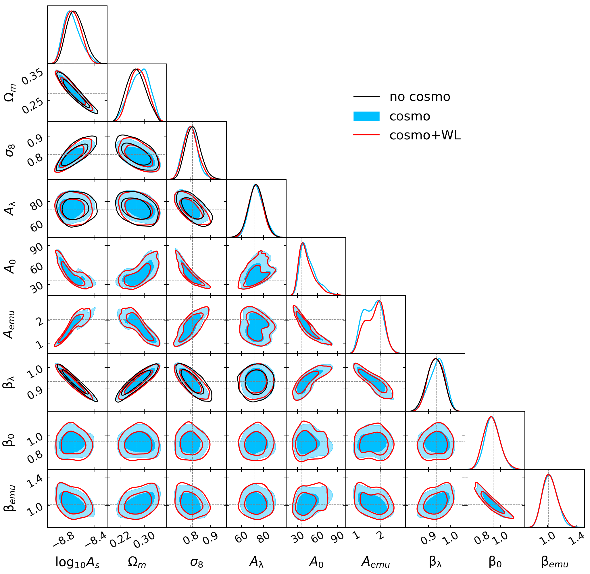
Figure 8: Contour plots at 68 and 95 per cent of confidence level for the three cases described in Sect. 5: no cosmo (black), cosmo (blue) and cosmo+WL (red) contours. The grey dashed lines represent the input values of parameters.

Table 3: Figure of merit in the $\Omega_{\rm m}\,$– $\sigma_{8}\,$ plane for the three cases of Fig. 8, plus the no cosmo + WL case. In the right column, normalised differences with respect to the no cosmo case.

Case	FoM	$\Delta$FoM/FoMnc
no cosmo	980	-
no cosmo + WL	993	0.01
cosmo	1044	0.06
cosmo + WL	1088	0.11

6 Conclusions

We tackled the problem of studying the satellite count $vs.$ halo mass relationship dependency on cosmological parameters and redshift and studied how such modelling could improve observational studies as mass-calibrations that use mass-richness relations. To this end we used FP Magneticum simulations Box1a C1–C15 (see Table 1) that were run with the same initial conditions but different cosmological parameters $\Omega_{m},\Omega_{b},\sigma_{8},h_{0}.$ We did not re-calibrate feedback parameters over the various runs, and in this study we focus on the effect of cosmological parameters on $N_{s}$ for a fixed feedback configuration. In particular:

• We showed that DMO and FP subhaloes depends differently from cosmological parameters, showing the importance of parametrising mass-richness relations with results from FP simulations rather than DMO ones.

• We built an emulator capable of predicting normalisation, log-slope and log-scatter of the high-mass power-law regime of the $N-M$ relation based on GPR modelling, in order to predict the number of satellites for a given cosmology. We estimated its error being within $\approx 20\%.$ This error is comparable with the same uncertainty predicted by the GPR, which ensures that the error estimation of the GPR is under control.

• We tested whether parametrising mass-richness relation with cosmological parameters can improve mass-calibration studies. The likelihood analysis on mock mass-calibration showed that the use of a cosmology-dependent HOD provides an improvement ($\sim$ 5 %) in the constraining power over a simple cosmology-independent HOD, which can be further improved ($\sim$ 10 %) if combined with multiple mass proxies, such as the weak lensing signal.

The study was carried out over a small number of cosmologies and with a resolution limited to the high-mass regime of haloes, and showed that mass-calibrations can benefit from modelling mass-richness relations with cosmological parameters from hydro-simulations. Future studies could focus on the dependency from cosmology of the radial distribution of substructures. The emulator log-slope predictions have a large uncertainty (see Figure 7 where $\beta$ shaded area spans between $\beta\in[0.9,1]$) which means there is the need for simulations over additional cosmological parameters and feedback parameters in order to improve GPR interpolation.

Appendix A Stellar mass cut

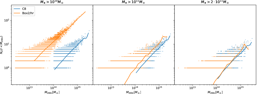
Figure 9: Galaxy abundance of HR (Box2/hr in orange) and MR (C8 in blue) simulations for varying minimum stellar mass of galaxies: $M_{\star}>10^{10}{\rm M}_{\odot}$ (left panel), $M_{\star}>10^{11}{\rm M}_{\odot}$ (middle panel), an $M_{\star}>2\cdot 10^{10}{\rm M}_{\odot}$ (right panel).

To build our HOD emulator, first of all we estimate which stellar mass cut to apply to the satellite count of our Box1a/mr C1–C15 simulations.

For this purpose we vary the stellar mass cut of both C8 and its HR counterpart (Box2/hr) until their $N_{s}-M$ relations statistically match. Figure 9 show convergence tests for stellar mass of C8 satellites. Left panel shows the $Ns-M$ relation of C8 and Box2/hr with the fiducial Box2/hr mass-cut $M_{\star}>10^{10}{\rm M}_{\odot}$ (as chosen in Anbajagane et al., 2020); central panel shows that a stellar mass cut $M_{\star}>10^{11}{\rm M}_{\odot}$ is not high enough to make C8 match its HR counter-part; right panel shows that a stellar mass cut $M_{\star}>2\cdot 10^{11}{\rm M}_{\odot}$ is capable reconciling the two simulations.

Appendix B Satellite abundance fit for each simulation

Table 4: Each row presents data for a given cosmolgy C1–C15 of Box1a/mr simulations, columns are grouped by redshift slices, and each redshift slice reports the halo mass cut $M_{\rm cut}$ in units of $10^{14}M_{\odot}$ and the corresponding parameters $A,B$ and $\sigma$ of Eq. (4). Upper rows present data for overdensity $\Delta_{v}ir$ and lower rows for overdensity 200c.

	$z=0.00$				$z=0.14$				$z=0.29$				$z=0.47$
	$M_{\rm cut}$	ln$A$	$\beta$	$\sigma$	$M_{\rm cut}$	ln$A$	$\beta$	$\sigma$	$M_{\rm cut}$	ln$A$	$\beta$	$\sigma$	$M_{\rm cut}$	ln$A$	$\beta$	$\sigma$
C1	-	-	-	-	-	-	-	-	-	-	-	-	-	-	-	-
C2	$15.2$	$-0.76$	$1.76$	$1.39$	$4.0$	$0.72$	$0.87$	$0.06$	-	-	-	-	-	-	-	-
C3	$4.8$	$0.73$	$1.05$	$0.03$	$4.5$	$0.87$	$0.98$	$0.04$	$4.5$	$0.98$	$0.98$	$0.04$	$5.0$	$1.05$	$0.88$	$0.05$
C4	$9.6$	$0.25$	$1.20$	$0.14$	$9.7$	$0.69$	$0.83$	$0.16$	-	-	-	-	$6.6$	$0.85$	$0.76$	$0.24$
C5	$8.4$	$0.49$	$1.01$	$0.08$	$7.1$	$0.50$	$1.15$	$0.07$	$9.6$	$0.49$	$1.23$	$0.10$	$7.5$	$0.33$	$1.45$	$0.10$
C6	$11.0$	$-0.41$	$1.62$	$0.33$	-	-	-	-	$7.8$	$-0.04$	$1.71$	$0.22$	-	-	-	-
C7	$16.3$	$-0.88$	$1.62$	$1.40$	$6.0$	$0.61$	$0.83$	$0.07$	$6.1$	$0.84$	$0.72$	$0.09$	$5.7$	$0.84$	$0.52$	$0.11$
C8	$4.3$	$0.78$	$0.98$	$0.03$	$4.8$	$0.93$	$0.90$	$0.03$	$5.1$	$1.01$	$0.89$	$0.03$	$4.6$	$1.04$	$1.01$	$0.04$
C9	$7.9$	$0.60$	$0.99$	$0.04$	$8.1$	$0.63$	$1.08$	$0.04$	$7.1$	$0.87$	$0.86$	$0.04$	$7.0$	$0.87$	$0.97$	$0.06$
C10	$4.8$	$0.73$	$1.02$	$0.02$	$4.0$	$0.88$	$1.00$	$0.02$	$3.6$	$0.99$	$1.02$	$0.02$	$4.5$	$1.13$	$0.94$	$0.02$
C11	$7.4$	$0.47$	$1.01$	$0.03$	$7.3$	$0.65$	$0.93$	$0.02$	$5.4$	$0.70$	$0.92$	$0.04$	$7.3$	$0.63$	$1.13$	$0.05$
C12	$4.8$	$0.56$	$1.00$	$0.02$	$6.1$	$0.70$	$0.98$	$0.02$	$7.1$	$0.83$	$0.95$	$0.03$	$5.9$	$0.85$	$1.02$	$0.04$
C13	-	-	-	-	-	-	-	-	-	-	-	-	-	-	-	-
C14	$10.4$	$0.18$	$1.06$	$0.03$	$9.4$	$0.31$	$1.04$	$0.03$	$7.6$	$0.38$	$1.02$	$0.03$	$10.2$	$0.24$	$1.33$	$0.07$
C15	$9.4$	$0.23$	$1.01$	$0.03$	$9.2$	$0.44$	$0.91$	$0.04$	$9.6$	$0.28$	$1.14$	$0.04$	$10.5$	$0.55$	$0.92$	$0.09$

Table 4 reports the fit parameters of average satellite abundance a function of halo mass, for all setups that had a $p-$value below $0.9$ and higher than $0.01.$ The problematic fits were the one at $z=0.67$ where few of them failed, probably because the resolution of our simulations are not always enough to reach this redshift. Only a total of $48$ fits were successful.

In order to fit the power-law halo-mass region of the satellite abundance relation, we imposed a halo mass cut (see Sec. LABEL:sec:conv) at $M_{\texttt{vir}}=3\cdot 10^{14}M_{\odot}$ for C8 simulation and scaled the mass cut to other simulations according to their baryon fraction. Some cuts have been modified in order to manually shrink or enlarge the halo range so to maximise the number of data points and yet do not cross the mass cut at low halo masses.

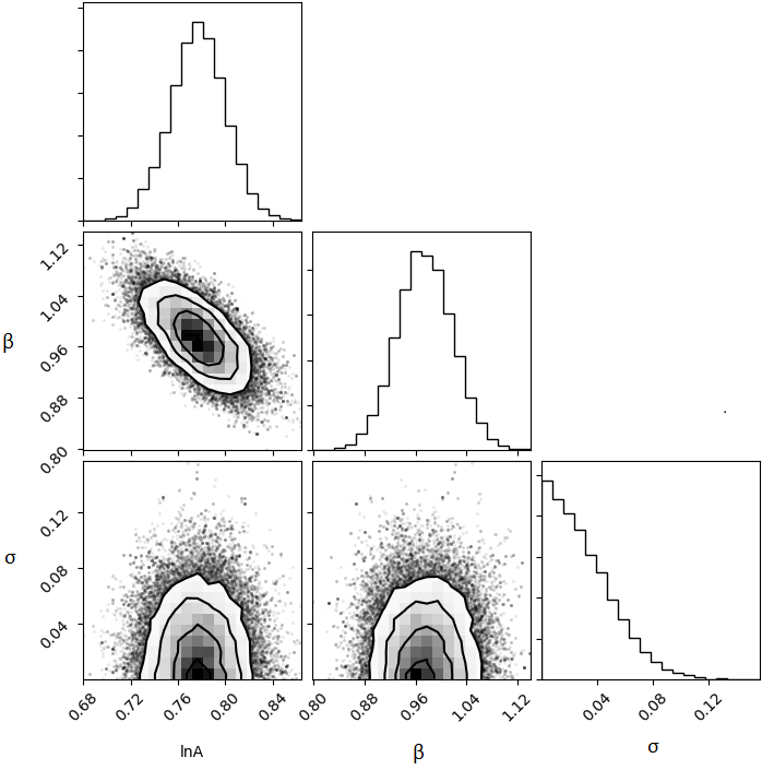
Figure 10: Posterior associated to Likelihood (5) for Box1a/mr C8 at $z=0$ for $\Delta=$ 200c. Parameters $A$ and $\beta$ are as in Eq. (4) and $\sigma$ is the fractional-scatter in the Likelihood.

Figure 10 shows the posterior of the fit for simulation Box1a/mr C8 $z=0.$ Here we can see that the fractional scatter $\sigma$ is consistent with zero.

Appendix C Cosmology dependent power-law fit posteriors

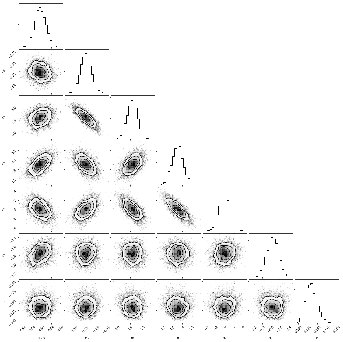
Figure 11: Posterior associated to Likelihood in Eq. (5). The parameter $lnA_{0}$ is the normalisation $0.64_{-0.03}^{+0.03}$ in Eq. 6), $\sigma$ is the gaussian-scatter of the fit, and $e_{m},e_{b},e_{\sigma},e_{h},e_{a}$ are, respectively, the exponents for logarithm of $\Omega_{m},\Omega_{b},\sigma_{8},h_{0},1/(1+z)$ divided by the respective pivot as disuccsed in Sec. 4.1.

In this appendix we report detail results of $A_{\mathrm{200c}}$ fit. To fit this, and, similarly, also $\beta$ and $\sigma$ for both $\Delta_{\mathrm{200c}}$ and $\Delta_{\mathrm{vir}},$ as in Eqs. (6) and (7), we maximised a Likelihood as follows:

$$\mathrm{ln}\mathcal{L}\left(\mathrm{ln}A_{0},e_{\mathbf{\theta}},\sigma\right)=-\frac{1}{2}\sum_{i}\left(\ln(2\pi\sigma^{2})+\left(\frac{\ln\ A_{\mathrm{200c}}\left(\mathrm{ln}A_{0},e_{\mathbf{\theta}},C_{i},z_{i}\right)-\ln\ A_{\mathrm{200c,i}}}{\sigma}\right)^{2}\right),$$ (15)

where $i$ runs over all setups, $C_{i}$ and $z_{i}$ are the cosmology and redshift of that setup, $A_{\mathrm{200c,i}}$ is the normalisation found in Section 4 for a given setup (and presented in Fig. LABEL:fig:hod_200c_megatabella_abs), $e_{\theta}$ is a set of exponents $(e_{m},e_{b},e_{\sigma},e_{h},e_{a})$ for the respective input parameters $\theta_{i}=(C_{i},a_{i})=(\Omega_{m,i},\Omega_{b,i},\sigma_{8,i},h_{0,i},a_{i}),$ and $\sigma$ is the fractional scatter, and $A_{\mathrm{200c}}$ has a power-law dependency from cosmological parameters, as follow

$$\mathrm{ln}\ A_{\mathrm{200c}}\left(\mathrm{ln}A_{0},e_{\mathbf{\theta}},\theta_{i}\right)=\mathrm{ln}A_{0}+\sum_{i}e_{i}\mathrm{ln}\frac{\theta_{i}}{\theta_{i,p}},$$ (16)

where the pivot values $\theta_{i,p}$ are presented in Sec. 4.2. Figure 11 shows an example of posterior distribution of parameters $($lnA${}_{0},e_{\theta},\sigma)$ for a single snapshot.

The evaluation of $\beta_{\textrm{200c}},\sigma_{\textrm{200c}},A_{\textrm{vir}},\beta_{\textrm{vir}}$ and $\sigma_{\textrm{200c}}$ have been performed in the same way as described above.

Appendix D Comparison with other simulation suites

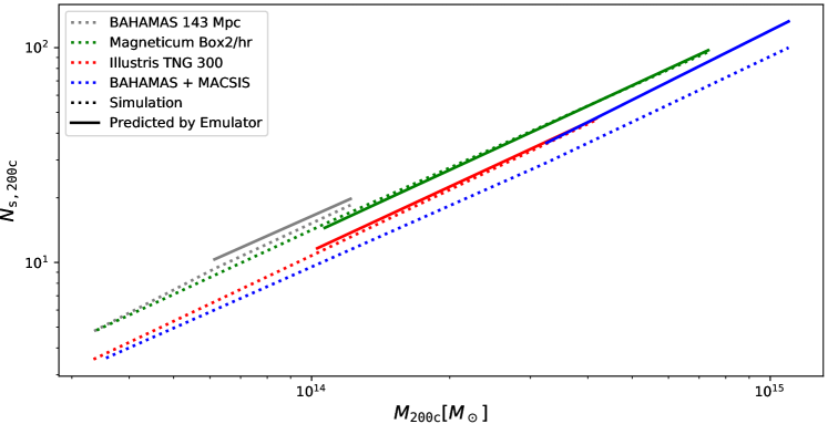
Figure 12: Dotted lines show number of satellites as a function of halo mass as taken from Fig. 2 of Anbajagane et al. (2020) for simulations BAHAMS high resolution (BM100, gray dashed line), Magneticum Box2b/hr (green dashed line), IllustrisTNG 300 (red dashed line) and BAHAMAS+MACSIS (gray dashed line). Solid lines are the same cosmologies as predicted by our emulator rescaled with Eq. (3). Normalisation of dashed lines is ordered as in the legend. Inset shows the distribution of Magneticum Box2/hr satellites and the respective prediction from $100$ realisations for each halo mass, both histogram refers to a mass range $10^{14}M_{\odot}<M_{\rm 200c}<1.2\cdot 10^{14}M_{\odot}$.

In this appendix we compare the results of our emulator against the mass-richness relations of some hydrodynamic simulations in the literature. Anbajagane et al. (2020) (see their Table 1 for more information) compared four hydrodynamic full-physics cosmological simulations: IllustrisTNG 300 (Pillepich et al., 2018; Nelson et al., 2018; Springel et al., 2018; Marinacci et al., 2018), BAHAMAS 143Mpc (McCarthy et al., 2017), BAHAMAS+MACSIS (Barnes et al., 2017) and Magneticum Box2/hr (Hirschmann et al., 2014; Dolag et al., 2009) and found a difference between $\langle N_{s}\rangle_{M}$ normalisation and slopes (see their Figure 2). In particular, their normalisation can differ of a factor $1.5,$ with BAHAMAS 143Mpc having the highest normalisation, Magneticum and BAHAMAS+MACSIS have similar slopes but different normalisation and IllustrisTNG has the highest log-slope and the only one that is steeper than unity.

Since these simulations have all different cosmological parameters, in this subsection we use the Emulator to test if the differences of satellite HODs of various simulations can be accounted, at least partially, by differences in their cosmological parameters.

In fact, BAHAMAS+MACSIS has parameters $\Omega_{m}=0.3175,f_{b}=0.154,\sigma_{8}=0.83,$ BAHAMAS has parameters $\Omega_{m}=0.279,f_{b}=0.166,\sigma_{8}=0.82$ and a redshift $z\approx 0.1,$ IllustrisTNG 300 has parameters $\Omega_{m}=0.31,f_{b}=0.16,\sigma_{8}=0.82,$ and MAGNETICUM has WMAP7 cosmological parameters.

Fig. 12 shows the $N_{\textrm{s}}$ $vs.$ halo mass of the four cosmological simulations and as predicted by our emulator at $z=0,$ when necessary, re-scaled for the different stellar mass cut according to Eq. (3)). We show the emulator prediction only for the high-mass power law regime.

The emulator matches the normalisation of IllustrisTNG and BAHAMS 143 Mpc. On the other hand, the emulator over-predicts BAHAMAS+MACSIS normalisation.