Causal connectability between quantum systems and the black hole interior in holographic duality

Abstract

In holographic duality an eternal AdS black hole is described by two copies of the boundary CFT in the thermal field double state. This identification has many puzzles, including the boundary descriptions of the event horizons, the interiors of the black hole, and the singularities. Compounding these mysteries is the fact that, while there is no interaction between the CFTs, observers from them can fall into the black hole and interact. We address these issues in this paper. In particular, we (i) present a boundary formulation of a class of in-falling bulk observers; (ii) present an argument that a sharp bulk event horizon can only emerge in the infinite $N$ limit of the boundary theory; (iii) give an explicit construction in the boundary theory of an evolution operator for a bulk in-falling observer, making manifest the boundary emergence of the black hole horizons, the interiors, and the associated causal structure. A by-product is a concept called causal connectability, which is a criterion for any two quantum systems (which do not need to have a known gravity dual) to have an emergent sharp horizon structure.

I Introduction

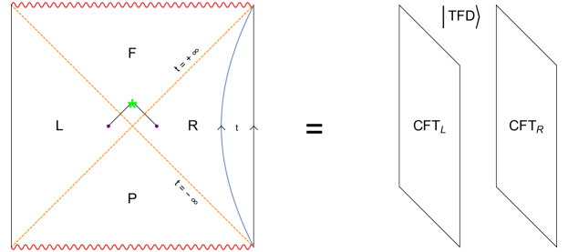
Figure 1: The Penrose diagram of an eternal black hole. The dashed lines are event horizons and the wavy lines are the singularities. Two observers from $R$ and $L$ can meet and interact behind the horizon despite the fact that there is no interaction between the left and right CFTs.

Understanding the emergence of causal structure in the bulk gravity theory from the boundary system in holographic duality has been an outstanding challenge. This issue can be formulated at many different levels. One of the most conspicuous features of bulk causal structure is the event horizon of a black hole. Understanding how these horizons and the regions beyond them emerge from the boundary theory should be a first step to address finer questions regarding bulk causal structure. Consider an eternal black hole, which is dual to two copies of the boundary CFT in the thermal field double state ${\lvert{\rm TFD}\rangle}$ Maldacena:2001kr . See Fig. 1. The boundary time, $t$, for each copy of the CFT coincides with the bulk Schwarzschild time which ends at the horizon. How is it then possible to construct an explicit evolution operator in the CFT describing a bulk observer originally in region $R$ falling through the horizon into the $F$ region? How should we interpret the black hole singularities in the bulk $F$ and $P$ regions from the boundary theory? Compounding these mysteries is the observation, first emphasized in Marolf:2012xe , that while there is no interaction between the two CFTs, observers from the $R$ and $L$ regions can fall into the $F$ region and interact with each other.

In this paper we address these questions. We first introduce a formulation of in-falling observers, which naturally leads to the concept of casual connectability: a boundary criterion for an emergent sharp horizon in the dual gravity system. We then provide an explicit boundary construction of a one-parameter family of unitary operators, $U(s)$, that play the role of evolution operators along an in-falling trajectory. More explicitly, $U(s)$ has the following properties:

1. It is generated by a Hermitian operator with a spectrum bounded from below.

2. Consider a scalar field $\phi(X)$ in the $R$ region, i.e. with $X\in R$, and its evolution under $U(s)$: $\Phi(X;s)\equiv U^{\dagger}(s)\phi(X)U(s)$. In this set-up, there exists an $s_{0}>0$, such that for $s>s_{0}$, $\Phi(X;s)$ can start having nonzero commutators with operators in CFT_L. Furthermore, $s_{0}$ coincides with the null Kruskal coordinate distance from $X$ to the horizon.

3. In the geometric optics limit (i.e. if the mass of $\phi$ is large), and with zero momentum along boundary spatial directions, $\Phi(X;s)=\phi(X_{s})$ where $X_{s}$ is a bulk point. For $s<s_{0}$, $X_{s}\in R$, while for $s>s_{0}$, $X_{s}\in F$.

The key to our discussion is the emergence, in the large $N$ limit of the boundary theory, of a type III₁ von Neumann algebraic structure from the type I boundary operator algebra and the half-sided modular translation structure associated to this type III₁ algebra. The black hole horizons, interiors, and singularities can all be understood as consequences of it. The type III₁ structure also sheds new light on the origin and nature of ultraviolet divergences in gravity. In this paper we outline the general ideas and the main results, leaving detailed expositions to LL .

II causal connectability: a boundary formulation of bulk horizon structure

In this section we introduce a boundary formulation of a class of bulk in-falling observers and the associated signature of a sharp horizon.

II.1 A boundary formulation of in-falling observers

In Marolf:2012xe a puzzle regarding the duality between the TFD state and the bulk eternal black hole geometry was raised. Consider an initial state of the form

$$\lvert{\Psi_{0}}\rangle=e^{iA_{L}}{\lvert{\rm TFD}\rangle}$$ (1)

where $A_{L}$ is a Hermitian operator in CFT_L and we assume that its insertion only changes the energy of the system by an $O(1)$ amount such that its backreaction on the geometry can be neglected. Since operators from the $R$ and $L$ sides commute, any measurement operator $M$ of the $R$ observer should commute with $e^{iA_{L}}$, i.e.

$${\left\langle{\Psi_{0}|M|\Psi_{0}}\right\rangle}={\left\langle{{\rm TFD}|M|{\rm TFD}}\right\rangle}$$ (2)

so the presence of $e^{iA_{L}}$ cannot have any consequence on the measurement. But this appears to be in contradiction with the ability of the insertion of $e^{iA_{L}}$ to influence a right observer who has fallen into the $F$ region of the eternal black hole geometry, see Fig. 1.

The above argument by itself does not directly pose a contradiction, as it assumes that the evolution of an in-falling observer from the $R$ region remains in CFT_R. It highlights, however, a seemingly counterintuitive requirement: for the identification of Fig. 1 to be correct, the description of an in-falling observer originally from the $R$ region must involve both the $R$ and $L$ systems. Indeed, from the causal structure of the black hole geometry, any operator in the $F$ region should involve degrees of freedom from both CFT_R and CFT_L. Thus whatever measurement operator, $M$, the observer uses in the $F$ region must involve degrees of freedom in CFT_L, and we cannot assume that $M$ commutes with $e^{iA_{L}}$.

In this paper we will show that the evolution of a family of in-falling observers on the gravity side can be described by a boundary “evolution operator” $U(s)=e^{-iGs},\,s\in{\mathbb{{R}}}$ that satisfies the following properties:

1. $G$ involves degrees of freedom from both CFT_R and CFT_L.

2. The Hermitian generator $G$ has a spectrum that is bounded from below,

   $$G\geq 0\ .$$ (3)

The first property is needed for the in-falling evolution $\Phi(X;s)\equiv U(-s)\phi(X)U(s)$ of a bulk operator $\phi(X)$ with $X\in R$ to have support in the $F$ region. The second property is natural from the following perspectives: (i) if we interpret the eigenvalues of $G$ as energies for a family of bulk observers, they should be bounded from below to ensure stability, (ii) the spectrum condition distinguishes $G$, as a generator of “time” flow, from operators generating spacelike displacements (such as momentum operators).

II.2 Sharp horizon structure only at infinite $N$

We will now show that the property (3) has important general implications regardless of the specific form of $U(s)$: a sharp event horizon can only emerge in the large $N$ limit of the boundary theory.

For this purpose, consider again the state (1), and the probability $p(s)$ for an in-falling observer originally from the $R$ region to observe the existence of $e^{iA_{L}}$ along their “trajectory” parameterized by $s$. To reproduce the causal structure of the black hole spacetime, $p(s)$ should have the form

$$p(s)=\begin{cases}0&s<s_{0}\cr\neq 0&s>s_{0}\end{cases},$$ (4)

with $s_{0}>0$, as it is only possible to detect the influence of $e^{iA_{L}}$ after the horizon has been crossed. The existence of such an $s_{0}$ and the non-smooth behavior of $p(s)$ at $s_{0}$ reflect the sharp causal structure from a sharp horizon.

There is a simple quantum mechanical argument Hegerfeldt:1993qe that the behavior (4) is in fact not possible. Denote the projection operator that can detect the possible existence of $e^{iA_{L}}$ as $P_{R}$. The subscript $R$ emphasizes that this is an operator in CFT_R. The probability $p(s)$ can then be written as

$$p(s)={\left\langle{\Psi_{0}|U^{\dagger}(s)P_{R}U(s)|\Psi_{0}}\right\rangle}={\left\langle{\phi(s)|\phi(s)}\right\rangle},\quad\lvert{\phi(s)}\rangle=P_{R}e^{-iGs}\lvert{\Psi_{0}}\rangle\ .$$ (5)

From (3), we can analytically continue $U(s)$ to the lower half complex-$s$ plane. Accordingly, $\lvert{\phi(s)}\rangle$ is a vector-valued analytic function of $s$ in the lower half complex $s$-plane, and is continuous along the real $s$-axis. Equation (4) means that $\lvert{\phi(s)}\rangle$ vanishes for a finite segment, $s\in(0,s_{0})$, of the real $s$-axis. Cauchy’s theorem then says if $\lvert{\phi(s)}\rangle$ is zero for any finite segment of $s$, it has to be identically zero for all $s$, incompatible with (4). Thus $p(s)$ can be zero only at isolated values of $s$ or identically zero, but cannot obey (4).

This argument is very general, independent of details of specific states or quantum systems. For example, the two CFTs can interact and have a bulk geometry described by a traversable wormhole Gao:2016bin .

Figure 2: Rindler regions of Minkowski spacetime.

Since the bulk gravity theory does have a sharp light cone, the above no-go argument must somehow be avoided in the duality relation. To understand a possible resolution, consider a closely related case: Rindler patches for a quantum field theory in Minkowski spacetime. See Fig. 2. If we discretize the theory by putting it on a lattice, the Minkowski vacuum $\lvert{\Omega}\rangle$ can be expressed as a TFD state for the $R$ and $L$ Rindler patches. In the discrete case there are no sharp light-cones. Any evolution on a lattice system has a small tail which gives rise to a nonzero commutator between two space-like separated operators. Indeed, in the discrete case, the above no-go argument applies: observers from the $R$ and $L$ Rindler systems are either always connected (for $p(s)$ having only isolated zeros) or can never be connected (for $p(s)$ identically zero). However, in the continuum limit, they are separated by sharp light-cones, and can meet in the $F$ region only after evolution by some nonzero $s_{0}$. This difference in the sharpness of the light-cone structure between the discrete case and the continuum limit can be attributed to a fundamental difference in the structure of their operator algebras. In the discrete case, the full Hilbert space factorizes into a tensor product of those of the $R$ and $L$ systems, and the operator algebras associated with the $R$ and $L$ systems are type I von Neumann algebras. In the continuum limit, there is no local Hilbert space associated with the $R$ or $L$ patch, and the local operator algebra associated to a Rindler region is a type III₁ von Neumann algebra. In the continuum case, the no-go argument does not apply, since for a type III₁ von Neumann algebra, there does not exist any projector $P_{R}$ that can be used to detect the influence of an $L$ observer. We expect that a type II von Neumann algebra will also be unable to describe operators outside of a sharp horizon but we will leave a rigorous mathematical proof elsewhere.

The above Rindler story suggests a way to go around the no-go argument regarding (4). The argument implicitly used that the full operator algebra of bounded operators of a CFT is type I (with the existence of a finite rank projector $P_{R}$), which is the case for the theory at finite $N$. But the duality with the classical black hole geometry and the associated sharp causal structure needs to hold only in the large $N$ limit. We will argue that in the $N\to\infty$ limit there is a pair of emergent type III₁ algebras, ${{\mathcal{M}}}_{R,L}$, in the boundary theory. The event horizons, black hole interior, and singularities are all consequences of this emergence.

Given that the conditions (4)–(5) for a sharp horizon structure cannot be defined for a type III₁ algebra, we need a generalization. We consider the function Buchholz:1994eb ; Yngvason:2014oia

$$F(s)=\sup\left\{\left|{\left\langle{\Psi_{0}|U^{\dagger}(s){{\mathcal{O}}}_{R}U(s)|\Psi_{0}}\right\rangle}-{\left\langle{{\rm TFD}|U^{\dagger}(s){{\mathcal{O}}}_{R}U(s)|{\rm TFD}}\right\rangle}\right|,\;{{\mathcal{O}}}_{R}\in{{\mathcal{M}}}_{R},\;||{{\mathcal{O}}}_{R}||\leq 1\right\}\ .$$ (6)

Existence of a sharp bulk horizon structure implies the existence of an $s_{0}>0$ and the behavior

$$F(s)=\begin{cases}0&s<s_{0}\cr\neq 0&s>s_{0}\end{cases}\ .$$ (7)

For infinitesimal $A_{L}$, the above equation is the same as the existence of an $s_{0}>0$ and ${{\mathcal{O}}}_{R}$ such that

$$[A_{L},U^{\dagger}(s){{\mathcal{O}}}_{R}U(s)]\neq 0\ ,\quad s>s_{0}\ .$$ (8)

The condition (7) can be used to describe an emergent sharp horizon for any two quantum systems and general states, even those without a known gravity dual. We will refer to two systems in a state which satisfies (7) as being causally connectable.

II.3 Emergent type III₁ von Neumann algebras

There is a natural candidate for the emergent type III₁ von Neumann algebra. Consider the vector space of products of single-trace operators of CFT${}_{R}.$ In the large $N$ limit, we can define an algebra of single-trace operators (see Leutheusser:2022bgi for details), ${{\mathcal{A}}}_{R},$ with respect to the thermal state, $\rho_{\beta}$ (${\beta}$ is the inverse temperature). We can build the GNS Hilbert space ${{\mathcal{H}}}^{\rm(GNS)}_{\rho_{\beta}}$ of ${{\mathcal{A}}}_{R}$ with respect to $\rho_{\beta}$. We denote the representation of ${{\mathcal{A}}}_{R}$ on ${{\mathcal{H}}}^{\rm(GNS)}_{\rho_{\beta}}$ as ${{\mathcal{M}}}_{R}$. Here are some features of ${{\mathcal{H}}}^{\rm(GNS)}_{\rho_{\beta}}$:

1. The representation of $\rho_{\beta}$ in ${{\mathcal{H}}}^{\rm(GNS)}_{\rho_{\beta}}$ is a pure state which we denote as $\lvert{\Omega_{0}}\rangle$. $\lvert{\Omega_{0}}\rangle$ is cyclic and separating for ${{\mathcal{M}}}_{R}$.

2. ${{\mathcal{H}}}^{\rm(GNS)}_{\rho_{\beta}}$ coincides with the GNS Hilbert space of the union of ${{\mathcal{A}}}_{L}$ and ${{\mathcal{A}}}_{R}$ with respect to ${\lvert{\rm TFD}\rangle}$. In particular, ${{\mathcal{M}}}_{L}$, the commutant of ${{\mathcal{M}}}_{R}$ in the operator algebra on ${{\mathcal{H}}}^{\rm(GNS)}_{\rho_{\beta}}$, can be viewed as the representation of ${{\mathcal{A}}}_{L}$ on ${{\mathcal{H}}}^{\rm(GNS)}_{\rho_{\beta}}$.

We conjecture that ${{\mathcal{M}}}_{R}$ and its commutant ${{\mathcal{M}}}_{L}$ are type III₁ in the large $N$ limit. An indication of this is the fact that the finite temperature spectral functions of single-trace operators have a continuous spectrum supported on the full real frequency axis despite the boundary CFT being defined on a compact space.

On the gravity side we quantize small metric and matter perturbations around the eternal black hole geometry. The resulting Fock space built on the Hartle-Hawking vacuum $\lvert{HH}\rangle$ is denoted as ${{\mathcal{H}}}_{\rm BH}^{\rm(Fock)}$ and the algebras of operators for the bulk theory in the $R$ and $L$ regions of the black hole are denoted as $\widetilde{{\mathcal{M}}}_{R},\widetilde{{\mathcal{M}}}_{L}$. Under the duality we identify:

$${{\mathcal{H}}}^{\rm(GNS)}_{\rho_{\beta}}={{\mathcal{H}}}_{\rm BH}^{\rm(Fock)},\quad\lvert{HH}\rangle=\lvert{\Omega_{0}}\rangle,\quad{{\mathcal{M}}}_{R}=\widetilde{{\mathcal{M}}}_{R},\quad{{\mathcal{M}}}_{L}=\widetilde{{\mathcal{M}}}_{L}\ .$$ (9)

The above identifications essentially consist of the statement of bulk reconstruction for the $R$ and $L$ regions of the black hole. They should hold perturbatively in the $1/N$ expansion (or bulk $G_{N}$ expansion). That ${{\mathcal{M}}}_{R,L}$ should be type III₁ is also required by the duality, as the bulk field algebras $\widetilde{{\mathcal{M}}}_{R,L}$, being associated with local bulk regions in a quantum field theory in curved spacetime, must be type III₁.

At the leading order in the $1/N$ expansion, the bulk algebras $\widetilde{{\mathcal{M}}}_{R,L}$ are generated by a free field theory while the boundary algebras ${{\mathcal{M}}}_{R,L}$ are generated by a generalized free field theory (since representations of single-trace operators on ${{\mathcal{H}}}^{\rm(GNS)}_{\rho_{\beta}}$ are generalized free fields). More explicitly, suppose a bulk field $\phi$ is dual to a boundary operator ${{\mathcal{O}}}$. The restrictions $\phi_{R,L}$ of $\phi$ to the $R,L$ regions of the black hole are dual respectively to the representations in ${{\mathcal{H}}}^{\rm(GNS)}_{\rho_{\beta}}$ of ${{\mathcal{O}}}_{R,L}$. They can be expanded in modes as (the sums below should be viewed as a proxy for integrals)

$$\phi_{R}(t,{\vec{x}},w)=\sum_{\omega,{\vec{k}}}e^{-i\omega t+i{\vec{k}}\cdot{\vec{x}}}v_{\omega{\vec{k}}}(w)\,a_{\omega{\vec{k}}}^{(R)},\qquad\phi_{L}(t,{\vec{x}},w)=\sum_{\omega,{\vec{k}}}e^{i\omega t-i{\vec{k}}\cdot{\vec{x}}}v_{\omega{\vec{k}}}(w)\,a_{\omega,{\vec{k}}}^{(L)},$$ (10)

$${{\mathcal{O}}}_{R}(t,{\vec{x}})=\sum_{\omega,{\vec{k}}}e^{-i\omega t+i{\vec{k}}\cdot{\vec{x}}}N_{\omega{\vec{k}}}\,a_{\omega{\vec{k}}}^{(R)},\qquad{{\mathcal{O}}}_{L}(t,{\vec{x}})=\sum_{\omega,{\vec{k}}}e^{i\omega t-i{\vec{k}}\cdot{\vec{x}}}N_{\omega{\vec{k}}}\,a_{\omega,{\vec{k}}}^{(L)},$$ (11)

where ${\vec{x}}$ collectively denotes the spatial coordinates on the boundary and $w$ denotes the bulk radial coordinate. $v_{\omega{\vec{k}}}(w)$ are the bulk mode functions and the $N_{\omega{\vec{k}}}$ are constants. The identifications (9) are reflected in the fact that $\phi$ and ${{\mathcal{O}}}$ share the same creation/annihilation operators $a_{\omega{\vec{k}}}^{(R,L)}$, and thus $\phi_{R,L}$ can be viewed as elements of boundary algebras ${{\mathcal{M}}}_{R,L}$.

The identifications (9) are shown in Fig. 3. In subsequent sections we will show that the type III₁ nature of ${{\mathcal{M}}}_{R,L}$ leads to the emergence of the $F$ and $P$ regions and the associated causal structure.

Figure 3: The identifications (9) establish duality of CFT_R,L with the exteriors of the black hole spacetime, but they do not directly say anything about the existence of the $F,P$ regions of a connected bulk.

III Emergent new times in the boundary

In this section we discuss how to generate new times in the boundary theory. Our main tool is half-sided modular translation Borchers:1991xk ; Wiesbrock:1992mg , and an extension of it. Suppose ${{\mathcal{M}}}$ is a von Neumann algebra and the vector $\Omega$ is cyclic and separating for ${{\mathcal{M}}}$. We denote the corresponding modular flow and conjugation operators as ${{\Delta}}_{{\mathcal{M}}}$ and $J_{{\mathcal{M}}}$. Now suppose there exists a von Neumann subalgebra ${{\mathcal{N}}}$ of ${{\mathcal{M}}}$ with the properties:

1. $\Omega$ is cyclic for ${{\mathcal{N}}}$ (it is automatically separating for ${{\mathcal{N}}}$ as ${{\mathcal{N}}}\subset{{\mathcal{M}}}$).

2. The half-sided modular flow of ${{\mathcal{N}}}$ under ${{\Delta}}_{{\mathcal{M}}}$ lies within ${{\mathcal{N}}}$, i.e.

   $${{\Delta}}^{-it}_{{\mathcal{M}}}{{\mathcal{N}}}{{\Delta}}^{it}_{{\mathcal{M}}}\subset{{\mathcal{N}}},\quad t\leq 0\ .$$ (12)

It can then be shown Borchers:1991xk ; Wiesbrock:1992mg ; Borchers:1998ye that there exists a unitary group $U(s),\,s\in{\mathbb{{R}}}$ with the following properties:

1. $U(s)$ has a positive generator, i.e.

   $$U(s)=e^{-iGs},\qquad G\geq 0$$ (13)

2. It leaves $\Omega$ invariant

   $$U(s)\Omega=\Omega,\quad\forall s\in{\mathbb{{R}}}$$ (14)

3. Half-sided inclusion

   $$U^{\dagger}(s){{\mathcal{M}}}U(s)\subseteq{{\mathcal{M}}},\quad\forall s\leq 0\ .$$ (15)

4. ${{\mathcal{N}}}$ can be obtained from ${{\mathcal{M}}}$ with an action of $U$

   $${{\mathcal{N}}}=U^{\dagger}(-1){{\mathcal{M}}}U(-1)$$ (16)

   and with ${{\mathcal{N}}}_{t}\equiv\Delta_{{{\mathcal{M}}}}^{-it}{{\mathcal{N}}}\Delta_{{{\mathcal{M}}}}^{it}$

   $$e^{iGs}{{\mathcal{N}}}_{t}e^{-iGs}={{\mathcal{N}}}_{f_{1}(s,t)},\quad f_{1}(s,t)=-{1\over 2\pi}\log(e^{-2\pi t}-s)\ .$$ (17)

We also note that

$$J_{{\mathcal{M}}}U(s)J_{{\mathcal{M}}}=U(-s)$$ (18)

and since ${{\mathcal{M}}}^{\prime}=J_{{\mathcal{M}}}{{\mathcal{M}}}J_{{\mathcal{M}}}$

$$U^{\dagger}(s){{\mathcal{M}}}^{\prime}U(s)\subseteq{{\mathcal{M}}}^{\prime},\quad s\geq 0\ .$$ (19)

The above structure is called half-sided modular translation and exists only if ${{\mathcal{M}}}$ is a type III₁ von Neumann algebra Borchers:1998 .

In our context, we take ${{\mathcal{M}}}={{\mathcal{M}}}_{R}$, ${{\mathcal{M}}}^{\prime}={{\mathcal{M}}}_{L}$, and $\Omega=\Omega_{0}$ (introduced in Sec. II.3), with the modular operator ${{\Delta}}_{{\mathcal{M}}}=\exp\left({\beta}(H_{R}-H_{L})\right)$ where $H_{R,L}$ are, respectively, the Hamiltonians of CFT_R,L. Thus modular evolutions of ${{\mathcal{M}}}_{R}$ under ${{\Delta}}_{{\mathcal{M}}}$ are simply the standard boundary time translations. By choosing different ${{\mathcal{N}}}$ we can construct different one-parameter group evolutions. These are candidates for new emergent “times” as the corresponding generators are bounded from below, as in (13). At leading order in the $1/N$ expansion, ${{\mathcal{M}}}_{R}$ and ${{\mathcal{M}}}_{L}$ are generated by generalized free fields. With the mode expansion (11), using (15) the action of $U(s)$ on ${{\mathcal{O}}}_{R}$ can be written in terms of a linear transform on $a_{\omega{\vec{k}}}^{(R)}$,

$$U^{\dagger}(s)a_{k}^{(R)}U(s)=\sum_{k^{\prime}}C_{kk^{\prime}}(s)a_{k^{\prime}}^{(R)},\quad k=(\omega,{\vec{k}}),\quad s\leq 0\ .$$ (20)

When $s>0$, $U(s)$ takes ${{\mathcal{O}}}_{R}$ outside ${{\mathcal{M}}}_{R}$ and the evolved operator is no longer covered by the theorem.

It turns out that when ${{\mathcal{M}}}_{R}$ is generated by generalized free fields, much more can be learned and it is possible to generalize the action of $U(s)$ to all values of $s$ LL :

1. The matrix $C_{kk^{\prime}}(s)$ can be determined up to a phase

   $$C_{kk^{\prime}}(s)={{\delta}}_{{\vec{k}},{\vec{k}}^{\prime}}\sqrt{{\sinh\pi|\omega^{\prime}|\over\sinh\pi|\omega|}}e^{i{{\gamma}}_{\omega}({\vec{k}})-i{{\gamma}}_{\omega^{\prime}}({\vec{k}})}(-s)^{-i(\omega-\omega^{\prime})}{{\Gamma}}(i(\omega-\omega^{\prime}))$$ (21)

   where the phase $e^{i{{\gamma}}_{\omega}({\vec{k}})}$ depends on the specific system and the choice of ${{\mathcal{N}}}$.

2. For all $s$, we can write

   $$U^{\dagger}(s)a_{k}^{({\alpha})}U(s)=\sum_{k^{\prime}}\sum_{{\beta}=R,L}\Lambda_{kk^{\prime}}^{{\alpha}{\beta}}(s)a_{k^{\prime}}^{({\beta})},\quad{\alpha}=R,L\ .$$ (22)

   For ${\alpha}=R$ and $s<0$, equation (22) reduces back to (20) which means that

   $$\Lambda_{kk^{\prime}}^{RR}(s)=C_{kk^{\prime}}(s),\quad\Lambda_{kk^{\prime}}^{RL}(s)=0,\quad s<0\ .$$ (23)

   $\Lambda^{R{\beta}}_{kk^{\prime}}(s)$ for $s>0$ can also be expressed in terms of $C_{kk^{\prime}}(s)$,

   $$\Lambda_{kk^{\prime}}^{RR}(s)={\sinh\pi\omega\over\sinh\pi\omega^{\prime}}C_{kk^{\prime}}(-s),\quad\Lambda_{kk^{\prime}}^{RL}(s)={\sinh\pi(\omega+\omega^{\prime})\over\sinh\pi\omega^{\prime}}C_{k,-k^{\prime}}(-s),\quad s>0\ .$$ (24)

   The action of $U(s)$ on ${{\mathcal{O}}}_{L}$, i.e. $\Lambda^{{\alpha}{\beta}}$ with ${\alpha}=L$, can be obtained from the relation

   $$\Lambda_{kk^{\prime}}^{{\alpha}{\beta}}(s)=\Lambda_{-k,-k^{\prime}}^{\bar{\alpha}\bar{\beta}}(-s)$$ (25)

   which is a consequence of (18) and ${{\mathcal{M}}}^{\prime}=J_{{\mathcal{M}}}{{\mathcal{M}}}J_{{\mathcal{M}}}$.

IV Emergence of the bulk Rindler horizon from the boundary

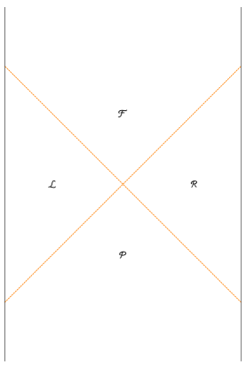
Figure 4: AdS Rindler regions of the bulk spacetime. The vertical lines denote the boundary and the dashed lines are Rindler horizons.

As a warmup for the black hole story we consider the emergence of the bulk Rindler horizon from the boundary system using the method outlined in the last section. Our input is the duality between the AdS Rindler region and the boundary CFT in the corresponding Rindler patch Hamilton:2006az ; Czech:2012be ; Morrison:2014jha . We will consider as an illustration, a bulk theory in the Poincare patch of AdS₃, dual to a two-dimensional boundary CFT on ${\mathbb{{R}}}^{1,1}$. The bulk spacetime contains two AdS Rindler regions which respectively have the two Rindler regions in ${\mathbb{{R}}}^{1,1}$ as their boundaries. The bulk theory in the bulk ${\mathcal{R}}/{{\mathcal{L}}}$ region in Fig. 4 is “reconstructible” from the boundary theory in the corresponding boundary $R/L$ region in Fig. 2. In this case, ${{\mathcal{M}}}_{R/L}$ is the algebra generated by single-trace operators in the $R/L$ Rindler regions. We note that going beyond the AdS Rindler horizon can be achieved by symmetries as the usual AdS isometries (which are dual to boundary conformal symmetries) can take an operator in the ${\mathcal{R}}$ region to the ${{\mathcal{F}}}$ region. But this example provides a nice illustration of the method of the last section and an interesting contrast for the discussion of the black hole case where such symmetries do not exist.

More explicitly, the metric for an AdS Rindler region can be written as

$$ds^{2}=\frac{R^{2}}{w^{2}}\left[-\left(1-w^{2}\right)d\eta^{2}+\left(1-w^{2}\right)^{-1}dw^{2}+d\chi^{2}\right]$$ (26)

with the Rindler horizon at $w=1$ and boundary at $w=0$. Consider a bulk scalar field $\phi$ dual to a boundary operator ${{\mathcal{O}}}$ with dimension ${{\Delta}}$. The restriction $\phi_{R}(X)$ of $\phi$ to the ${\mathcal{R}}$ region (with $X=(\eta,w,\chi)$) can be expanded in modes as

$$\phi_{R}(X)=\int\frac{d^{2}k}{(2\pi)^{2}}\,e^{ik\cdot x}v_{k}(w)a_{k}^{(R)},\quad k=(\omega,q),\quad k\cdot x=-\omega\eta+q\chi$$ (27)

$$v_{k}(w)=N_{k}f_{k}(w),\quad q_{\pm}={{\frac{1}{2}}}({{\Delta}}+i(\omega\pm q)),\quad\bar{q}_{\pm}={{\frac{1}{2}}}({{\Delta}}-i(\omega\pm q))$$ (28)

$$N_{k}={\sqrt{\sinh\pi|\omega|}\over\sqrt{2\pi}{{\Gamma}}({{\Delta}})}\left|\Gamma\left(q_{+}\right)\Gamma\left(q_{-}\right)\right|,\quad f_{k}(w)=w^{\Delta}(1-w^{2})^{-i\omega/2}{}_{2}F_{1}\left(\bar{q}_{-},\bar{q}_{+};\Delta;w^{2}\right)\ .$$ (29)

The $a_{k}^{(R)}$ are creation (for $\omega<0$) and annihilation (for $\omega>0$) operators of the boundary generalized free field theory in the $R$ region, and thus $\phi_{R}(X)$ can be interpreted as an operator in the boundary theory. There is a similar “bulk reconstruction” equation for $\phi_{L}$ in terms of $a_{k}^{(L)}$.

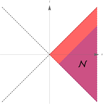
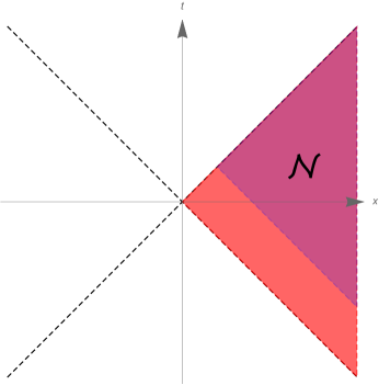
Figure 5: Boundary subregions that are used for the construction of a one-parameter group of unitaries implementing bulk Poincaré $U-$ and $V-$translations, respectively. $t,x$ are boundary Minkowski coordinates.

Our goal is to use the boundary theory in the $R,L$ regions and (27) to reconstruct the bulk theory in the full Poincare AdS spacetime, including the ${{\mathcal{F}}}$ and ${{\mathcal{P}}}$ regions in Fig. 4. For this purpose we take ${{\mathcal{M}}}={{\mathcal{M}}}_{R}$, which is type III₁ as it is the local algebra for a Rindler region. We take ${{\mathcal{N}}}$ to be the algebra of operators in the region indicated in Fig. 5, corresponding to a null shift in one of the boundary light cone directions. Clearly ${{\mathcal{N}}}\subset{{\mathcal{M}}}$. For the choice of the left plot of Fig. 5, the corresponding $C_{kk^{\prime}}$ can be computed explicitly in the boundary theory. It has the form of (21) with

$$e^{i{{\gamma}}_{k}}={{{\Gamma}}(\bar{q}_{+})\over|{{\Gamma}}(\bar{q}_{+})|}\ .$$ (30)

From our earlier discussion this fully determines $\Lambda_{kk^{\prime}}^{{\alpha}{\beta}}(s)$ for all $s$. We can then work out how a bulk field (27) transforms under the evolution of $U(s)$. From the form of $v_{k}(w)$ it can be shown that for $s<s_{0}\equiv e^{-\eta+\chi}\sqrt{1-w^{2}}$

$$U^{\dagger}(s)\phi_{R}(X)U(s)=\phi_{R}(X_{s}),$$ (31)

where $X_{s}=(\eta_{s},\chi_{s},w_{s})$ with

$$w_{s}={w\over\sqrt{1-a_{s}}},\quad e^{\eta_{s}}={e^{\eta}\sqrt{1-w^{2}}\over\sqrt{1-a_{s}-w^{2}}},\quad e^{\chi_{s}}=e^{\chi}\sqrt{1-a_{s}},\quad a_{s}\equiv{s(1-w^{2})\over s_{0}}\ .$$ (32)

It can be readily checked that the above transformation precisely corresponds to a shift $U\to U+s$ of the Poincare null coordinate $U$, in terms of which the AdS metric reads

$$ds^{2}={R^{2}\over z^{2}}\left(-dt^{2}+dx^{2}+dz^{2}\right)={R^{2}\over z^{2}}\left(-dUdV+dz^{2}\right),\quad U=t-x,\quad V=t+x\ .$$ (33)

In particular, $-s_{0}$ is the value of the $U$ coordinate for the point $X$, and thus $s=s_{0}$ takes $X$ to the Rindler horizon. The transformation (31) is smooth at $s=s_{0}$, and when $s>s_{0}$ the right hand side also involves $a_{k}^{(L)}$ with

$$U^{\dagger}(s)\phi_{R}(X)U(s)=\phi_{F}(X_{s}),$$ (34)

where $X_{s}\in{{\mathcal{F}}}$ is again obtained by a null Poincare shift $U\to U+s$ and $\phi_{F}(X_{s})$ is the restriction of $\phi$ to the ${{\mathcal{F}}}$ region.

Similarly, choosing ${{\mathcal{N}}}$ as in the right plot of Fig. 5 gives rise to null Poincare translations $V\to V+s$.

The above construction explicitly demonstrates the emergence of the AdS Rindler horizons and the associated bulk causal structure from the boundary theory.

V Emergence of the black hole event horizon and Kruskal time

We now consider the emergence of the interior of the black hole from the boundary theory. The bulk theory in the eternal black hole geometry is now dual to two copies of the boundary theory on ${\mathbb{{R}}}\times S^{d-1}$ in the state ${\lvert{\rm TFD}\rangle}$. For illustration we again take $d=2$, i.e. a BTZ black hole Banados:1992wn , whose metric has exactly the same form as (26) but now with $\chi$ compact. The bulk reconstruction formula for a scalar field $\phi$ in the $R$ region has the same form as (27) except that the integration over $q$ is replaced by a discrete sum. The corresponding boundary manifold, instead of being a Rindler patch of Minkowski spacetime, is given by ${\mathbb{{R}}}\times S^{1}$. We take ${{\mathcal{M}}}={{\mathcal{M}}}_{R}$, the algebra generated by single-trace operators in CFT_R. The corresponding algebra of bulk fields in the $R$ region is $\widetilde{{\mathcal{M}}}_{R}$.

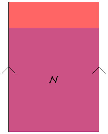
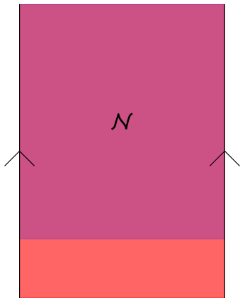
Figure 6: The left plot gives the boundary subregion that is used for the construction of a one-parameter group of unitaries that carries an observer from the $R$ region across the future horizon of the black hole into the $F$ region. The boundary is ${\mathbb{{R}}}\times S^{1}$ (vertical boundaries in the figure are identified). The relevant subalgebra is that generated by single-trace operators supported up to some maximum value of the boundary time (which we will take to be $\eta=0$). The right plot is the boundary subregion used to construct the unitaries to carry an observer from the $R$ region across the past horizon of the black hole. The relevant subalgebra is that generated by single-trace operators supported at boundary times greater than some minimum value (which we will again take to be $\eta=0$).

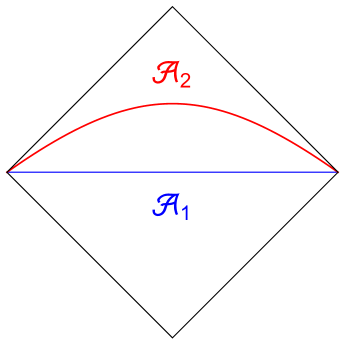
Figure 7: In a generalized free field theory, the algebras ${{\mathcal{A}}}_{1}$ and ${{\mathcal{A}}}_{2}$ of the two different slices shown are inequivalent, even though they share a causal diamond.

In this case the constructions of last section no longer apply since when $\chi$ is compact, a boundary null shift as in Fig. 5 is not well defined. We will instead take ${{\mathcal{N}}}$ to be the operator algebra associated with the region indicated in the left plot of Fig. 6. To see that this is a sensible choice, it should be emphasized that generalized free fields do not satisfy any Heisenberg equations, and thus the algebras generated by them are not defined by causal diamonds. For example, the algebras associated with the two spacetime regions in Fig. 7 are inequivalent, even though they share the same causal diamond. The state ${\lvert{\rm TFD}\rangle}$ is clearly separating with respect to ${{\mathcal{N}}}$. While we do not have a rigorous mathematical proof, we will assume that it is also cyclic with respect to ${{\mathcal{N}}}$.

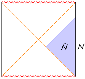
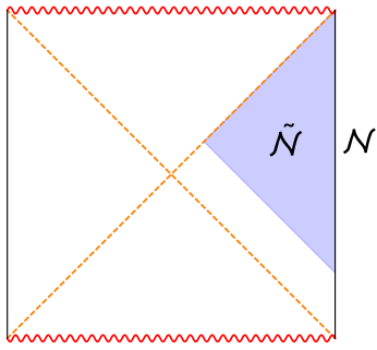
Figure 8: The respective proposed bulk duals for the boundary subregions indicated in Fig. 6.

Finding $U(s)$ for this choice of ${{\mathcal{N}}}$ is now difficult. We will find its explicit form by proposing a candidate for the dual of ${{\mathcal{N}}}$ in the bulk. We propose that the operator algebra ${{\mathcal{N}}}$ is dual to the algebra of bulk fields in the region $\widetilde{{\mathcal{N}}}$ shown in Fig. 8. This proposal is natural as this is the causal wedge associated with that part of the boundary, and we conjecture it is also the bulk subregion whose associated operator algebra is equal to ${{\mathcal{N}}}$. We emphasize that the bulk dual here is not defined by an extremal surface prescription. We will provide further support for this identification below.

Using the bulk theory it is then possible to explicitly construct $U(s)$. For a bulk scalar field (27) the corresponding matrix $C_{kk^{\prime}}$ again has the form (21) with phase ${{\gamma}}$ given by

$$e^{i{{\gamma}}_{k}}=e^{i{{\delta}}_{k}}{|{{\Gamma}}(i\omega)|\over{{\Gamma}}(i\omega)}=e^{-i\omega\log 2}{{{\Gamma}}(\bar{q}_{-}){{\Gamma}}(\bar{q}_{+})\over|{{\Gamma}}(\bar{q}_{-}){{\Gamma}}(\bar{q}_{+})|}$$ (35)

where $e^{i{{\delta}}_{k}}$ is the phase shift for the scalar field at the horizon, and in the second equality we have given the explicit expression for the case of a BTZ black hole ($\bar{q}_{\pm}$ was defined earlier in (28)). More explicitly, ${{\delta}}_{k}$ can be read from the behavior of bulk mode function $v_{k}(w)$ near $w=1$

$$v_{k}(w)={1\over\sqrt{2|\omega|}}\left(e^{-i\omega\xi+i\delta_{k}}+e^{i\omega\xi-i\delta_{k}}\right),\quad w\to 1,\quad\xi={{\frac{1}{2}}}\log{1-w\over 1+w}$$ (36)

where $\xi$ is the tortoise coordinate. With the explicit form of $C_{kk^{\prime}}$ we can then work out the action of $U(s)$ on $\phi_{R}(X)$. The resulting operator $\Phi(X,s)\equiv U^{\dagger}(s)\phi_{R}(X)U(s)$ has the following properties:

1. It is not a local operator, but may be understood as $\phi$ smeared over a certain spacetime region. Writing $X=(\eta_{0},\chi_{0},w_{0})$ in terms of Kruskal coordinates, $X=(U_{0},V_{0},\chi_{0})$ (see Appendix A for the transformation between the coordinates of (26) and the Kruskal coordinates), we find $\Phi(X;s)$ is supported only for $U<U_{0}+s$. In particular, for $s<s_{0}\equiv-U_{0}$, $\Phi(X;s)\in\widetilde{{\mathcal{M}}}_{R}$, while for $s>s_{0}$, $a_{k}^{(L)}$ is now also involved.

2. For $X$ near the horizon, i.e. $-U_{0}\ll 1$, $U(s)$ acts as a point-wise $U$ translation, $\Phi(X;s)=\phi(X_{s})$ with $X_{s}=(U_{0}+s,V_{0},\chi_{0})$, to leading order in $-U_{0}$.

3. For general points $X_{1}\in R$ and $X_{2}\in L$, we find that

   $$[U^{\dagger}(s)\phi_{R}(X_{1})U(s),\phi_{L}(X_{2})]=0$$ (37)

   for $s<s_{12}\equiv-U_{1}+U_{2}$, but the commutator becomes nonzero when $s>s_{12}$, precisely reproducing the casual structure expected from the black hole geometry. See Fig. 9. From the boundary theory perspective, this means that the two boundary systems are casually connectable in the sense of (8).

4. Acting on an operator ${{\mathcal{O}}}_{R}$ at boundary point $(\eta_{0},\chi_{0})$ it is a nonlocal transformation with support only for $\eta<-\log(e^{-\eta_{0}}-s)$. This agrees with (17), and provides a nontrivial consistency check of the identification of the shaded region $\widetilde{{\mathcal{N}}}$ in Fig. 8 as the bulk dual of the boundary subalgebra ${{\mathcal{N}}}$.

5. In the large $\Delta$ limit, with $q=0$ (i.e. if we dimensionally reduce both the bulk and boundary theories on the circle $\chi$), the transformation is point-wise

   $$\Phi(X;s)=\lambda_{X}\phi(X_{s}),\quad\lambda_{X}=\sqrt{1-s\sqrt{1-w_{0}^{2}}e^{\eta_{0}}}$$ (38)

   with $X_{s}$ given by

   $$e^{2\eta_{s}}={e^{2\eta_{0}}\over 1-{2se^{\eta_{0}}\over\sqrt{1-w^{2}_{0}}}+s^{2}e^{2\eta_{0}}},\quad w_{s}={w_{0}\over 1-s\sqrt{1-w^{2}_{0}}e^{\eta_{0}}}\ .$$ (39)

   The above transformation can be expressed in terms of Kruskal coordinates as

   $$U_{s}=U_{0}+s,\qquad V_{s}={V_{0}\over 1-sV_{0}}\ .$$ (40)

   The trajectories following from (40) are shown in Fig. 10.

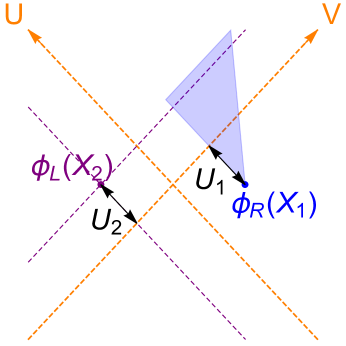
Figure 9: When a bulk field $\phi_{R}(X_{1})$ with $X_{1}\in R$ is transported by a null Kruskal coordinate distance $-U_{1}+U_{2}$ (since $U_{1}<0$), it enters the lightcone of $\phi_{L}(X_{2})$. The shaded region is a cartoon for the spread of $\Phi(X_{1};s)$. The orange dashed lines are event horizons, and the purple dashed lines give the light cones of $X_{2}$. The boundaries and singularities suppressed in the figure.

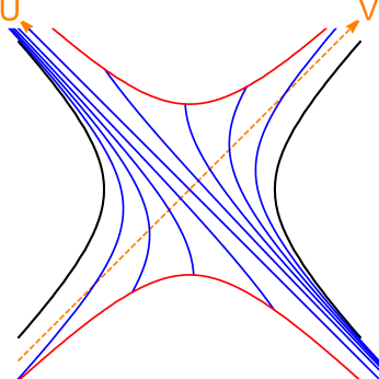
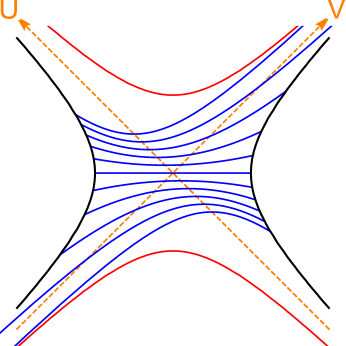
Figure 10: The left plot gives trajectories of (40). The right plot gives constant $s$ surfaces evolved from the $\eta=0$ slice. The orange dashed lines are the event horizons, black solid lines are the boundaries, while the red solid lines are the singularities.

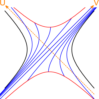
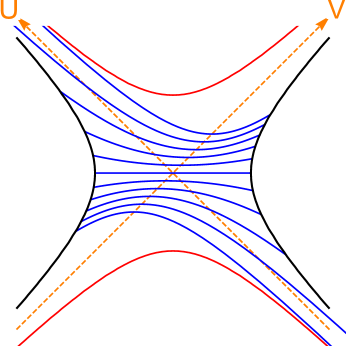
Figure 11: The counterparts of Fig. 10 when using ${{\mathcal{N}}}$ as in the right plot of Fig. 6.

By choosing ${{\mathcal{N}}}$ to be the algebra associated with region in the right plot of Fig. 6, we can similarly construct unitary evolutions as above but with the roles of Kruskal $U$ and $V$ swapped. See Fig. 11 for the corresponding flow trajectories.

VI Discussion

VI.1 Possible choices of $U(s)$ and more general states

In Sec. V we discussed two possible choices of ${{\mathcal{N}}}$ and the corresponding $U(s)$. These are only the simplest choices. There are an infinite number of others. For example, for both plots in Fig. 6 instead of letting the region describing ${{\mathcal{N}}}$ be bounded by the $\eta=0$ slice on the boundary, we can choose a slice $\eta=f(\chi)$ where $\chi$ is the boundary spatial coordinate and $f$ an arbitrary periodic function. Alternatively, instead of taking the cyclic and separating vector $\lvert{\Omega}\rangle$ to be the “vacuum” $\lvert{\Omega_{0}}\rangle$ of the GNS Hilbert space dual to the bulk Hartle-Hawking vacuum we can also choose other $\lvert{\Omega}\rangle$. The simplest possibilities are obtained by acting on $\lvert{\Omega_{0}}\rangle$ unitaries from ${{\mathcal{M}}}_{R}$ and ${{\mathcal{M}}}_{L}$, i.e.

$$\lvert{\Omega}\rangle=V_{L}W_{R}\lvert{\Omega_{0}}\rangle,\quad V_{L}\in{{\mathcal{M}}}_{L},\quad W_{R}\in{{\mathcal{M}}}_{R}$$ (41)

which results in a $U(s)=V_{L}W_{R}U_{0}(s)W_{R}^{\dagger}V_{L}^{\dagger}$ with $U_{0}$ denoting the evolution operator corresponding to $\lvert{\Omega_{0}}\rangle$.

Our discussion can also be generalized to more general entangled states of CFT_R and CFT_L. A simple variant is to act on ${\lvert{\rm TFD}\rangle}$ by a left unitary $U_{L}$ which does not change the reduced density matrix $\rho_{\beta}$ of the CFT_R, i.e.

$$\lvert{\Psi}\rangle=U_{L}{\lvert{\rm TFD}\rangle}\ .$$ (42)

The story depends on whether $\lvert{\Psi}\rangle$ lies in the GNS Hilbert space built from ${\lvert{\rm TFD}\rangle}$. If $\lvert{\Psi}\rangle$ lies in the GNS Hilbert space, the bulk geometry is still described by the eternal black hole, now with some small excitations on the left due to insertion of $U_{L}$. The construction of $U(s)$ is the same as that for ${\lvert{\rm TFD}\rangle}$. In particular, there are an infinite number of choices of $\lvert{\Omega}\rangle$ as in (41). When $\lvert{\Psi}\rangle$ does not lie in the GNS Hilbert space, for example if $U_{L}$ changes the energy of the system by an amount which scales with $N$, the story is different. We need to work with the GNS space ${{\mathcal{H}}}_{\Psi}^{\rm GNS}$ associated with $\lvert{\Psi}\rangle$, which does not overlap with that associated with ${\lvert{\rm TFD}\rangle}$, and the corresponding representations ${{\mathcal{M}}}_{L,R}$ of single-trace operator algebras are also different from those of associated with ${\lvert{\rm TFD}\rangle}$. In this case there is no simple relation between $U(s)$ for $\lvert{\Psi}\rangle$ with those for ${\lvert{\rm TFD}\rangle}$ as they act on different GNS Hilbert spaces.

VI.2 Interpretation of the black hole singularity

From a generic bulk point $X\in R$, the flow (40) reaches the future singularity for a finite value of $s$. Since we expect in general that the wave function of a bulk field should become singular at the singularity, the presence of the singularity in the black hole geometry should imply that the emergent evolution $U(s)$ breaks down at finite values of $s$.

It is instructive to contrast the nature of the $U(s)$ of Sec. V with those of Sec. IV. In the discussion of Sec. IV, while we also used generalized free fields, the evolution operator $U(s)$ from the choices of ${{\mathcal{N}}}$ in Fig. 5 can be defined for the full theory at finite $N$. Thus $U(s)$ there should be well defined for $s\in(-\infty,+\infty)$. But the $U(s)$ of Sec. V only exists in the large $N$ limit, so the associated sharp horizon and interior (i.e. causal connectability from the boundary perspective) only exist in this limit. We can thus interpret the black hole singularity as a limitation on this emergent causal connectability; the connection of left and right observers cannot be extended indefinitely, unlike the case of AdS Rindler.

VI.3 The nature of UV divergences in gravity and factorization of modular operator

The entanglement entropy, $S_{R}$, of CFT_R in ${\lvert{\rm TFD}\rangle}$ is given by the generalized entropy on the gravity side

$$S_{R}={A\over 4G_{N}}+{\mathcal{S}}_{R}$$ (43)

where $A$ is the horizon area and ${\mathcal{S}}_{R}$ denotes entropy of matter fields in the $R$ region of the black hole geometry. There is also a relation between the corresponding modular operators Jafferis:2015del

$$H_{R}={\hat{A}\over 4G_{N}}+K_{R}$$ (44)

where $H_{R}$ is the Hamiltonian of CFT_R, $K_{R}$ is the modular operator for the bulk field algebra $\widetilde{{\mathcal{M}}}_{R}$ and $\hat{A}$ is the horizon area operator. $K_{R}$ suffers from bulk UV divergences as does ${\mathcal{S}}_{R}$. But the left hand sides of (43) and (44) are well defined. For these expressions to make sense, the UV divergences of $K_{R}$ and ${\mathcal{S}}_{R}$ must exactly be canceled by those in $G_{N}$ (understood as the bare coupling) to all orders in $G_{N}$ expansion.

From the identification of ${{\mathcal{M}}}_{R}$ and $\tilde{{\mathcal{M}}}_{R}$, $K_{R}$ can be identified with the modular operator of ${{\mathcal{M}}}_{R}$, and its divergences must then originate from the emergent type III₁ structure. This provides a different perspective on the bulk UV divergences and renormalization of the Newton constant $G_{N}$. The divergence in $K_{R}$ is a reflection that, in a type III₁ algebra, the modular operator for ${{\mathcal{M}}}_{R}$ cannot be factorized into those for the $R$ and $L$ systems. Since the algebra for the full CFT is type I, the corresponding modular operator is factorizable, and thus the area term in (44) must “restore” the algebra from type III₁ to type I.

VI.4 Some future directions

There are many more questions to be understood and we mention a few here. It is clearly of great interest to understand better the emergence of the type III₁ structure in the large $N$ limit, and what becomes of the in-falling evolution operators at finite $N$. In particular, it is important to understand more precisely the emergence of singularities in the boundary theory. The discussion here should also be generalizable to single-sided black holes including evaporating ones. We expect such constructions can shed new light on the information loss problem. We also expect that the manner in which an in-falling time emerges from the boundary theory here should teach us valuable lessons about holography for asymptotically flat and cosmological spacetimes. This should be especially helpful for understanding time in cosmological spacetimes including de Sitter.

Acknowledgements

We would like to thank Netta Engelhardt, Hao Geng, Daniel Harlow, Gary Horowitz, Daniel Jafferis, Lampros Lamprou, Juan Maldacena, Donald Marolf, Leonard Susskind, Aron Wall, and Edward Witten for discussions, and Horacio Casini for communications. This work is supported by the Office of High Energy Physics of U.S. Department of Energy under grant Contract Number DE-SC0012567 and and DE-SC0019127. SL acknowledges the support of the Natural Sciences and Engineering Research Council of Canada (NSERC).

Appendix A Kruskal coordinates for the BTZ spacetime

For the BTZ metric (26), the tortoise coordinate is given by

$$\xi=-\int{dw\over 1-w^{2}}={{\frac{1}{2}}}\log{1-w\over 1+w}\ .$$ (45)

The Kruskal coordinates in the right exterior region are

$$U=-e^{\xi-\eta}=-\sqrt{1-w\over 1+w}e^{-\eta},\quad V=e^{\xi+\eta}=\sqrt{1-w\over 1+w}e^{\eta},$$ (46)

$$-e^{2\xi}=UV={w-1\over w+1},\quad w={1+UV\over 1-UV},\quad e^{2\eta}=-{V\over U}\ .$$ (47)

The singularity lies at $UV=1$ and the boundary at $UV=-1$. The event horizons are at $U,V=0$.

References

- (1) J. M. Maldacena, JHEP 04, 021 (2003) [arXiv:hep-th/0106112 [hep-th]].
- (2) J. Maldacena and X. L. Qi, [arXiv:1804.00491 [hep-th]].
- (3) H. W. Lin, J. Maldacena and Y. Zhao, JHEP 08, 049 (2019) [arXiv:1904.12820 [hep-th]].
- (4) D. Marolf and A. C. Wall, Class. Quant. Grav. 30, 025001 (2013) [arXiv:1210.3590 [hep-th]].
- (5) P. Kraus, H. Ooguri and S. Shenker, Phys. Rev. D 67, 124022 (2003) [arXiv:hep-th/0212277 [hep-th]].
- (6) L. Fidkowski, V. Hubeny, M. Kleban and S. Shenker, JHEP 02, 014 (2004) [arXiv:hep-th/0306170 [hep-th]].
- (7) G. Festuccia and H. Liu, JHEP 04, 044 (2006) [arXiv:hep-th/0506202 [hep-th]].
- (8) T. Hartman and J. Maldacena, JHEP 05, 014 (2013) [arXiv:1303.1080 [hep-th]].
- (9) H. Liu and S. J. Suh, Phys. Rev. Lett. 112, 011601 (2014) [arXiv:1305.7244 [hep-th]].
- (10) H. Liu and S. J. Suh, Phys. Rev. D 89, no.6, 066012 (2014) [arXiv:1311.1200 [hep-th]].
- (11) L. Susskind, Fortsch. Phys. 64, 24-43 (2016) [arXiv:1403.5695 [hep-th]].
- (12) M. Grinberg and J. Maldacena, JHEP 03, 131 (2021) [arXiv:2011.01004 [hep-th]].
- (13) Y. Zhao, JHEP 21, 144 (2020) [arXiv:2011.06016 [hep-th]].
- (14) F. M. Haehl and Y. Zhao, JHEP 06, 056 (2021) [arXiv:2102.05697 [hep-th]].
- (15) F. M. Haehl and Y. Zhao, Phys. Rev. D 104, no.2, L021901 (2021) doi:10.1103/PhysRevD.104.L021901 [arXiv:2104.02736 [hep-th]].
- (16) F. M. Haehl, A. Streicher and Y. Zhao, JHEP 08, 134 (2021) doi:10.1007/JHEP08(2021)134 [arXiv:2105.12755 [hep-th]].
- (17) M. Van Raamsdonk, Gen. Rel. Grav. 42, 2323-2329 (2010) [arXiv:1005.3035 [hep-th]].
- (18) J. Maldacena and L. Susskind, Fortsch. Phys. 61, 781-811 (2013) [arXiv:1306.0533 [hep-th]].
- (19) D. L. Jafferis and L. Lamprou, [arXiv:2009.04476 [hep-th]].
- (20) A. Hamilton, D. N. Kabat, G. Lifschytz and D. A. Lowe, Phys. Rev. D 73, 086003 (2006) [arXiv:hep-th/0506118 [hep-th]].
- (21) A. Hamilton, D. N. Kabat, G. Lifschytz and D. A. Lowe, Phys. Rev. D 75, 106001 (2007) [erratum: Phys. Rev. D 75, 129902 (2007)] [arXiv:hep-th/0612053 [hep-th]].
- (22) K. Papadodimas and S. Raju, JHEP 10, 212 (2013) [arXiv:1211.6767 [hep-th]].
- (23) Y. Nomura, Phys. Rev. D 99, no.8, 086004 (2019) [arXiv:1810.09453 [hep-th]].
- (24) Y. Nomura, Phys. Rev. D 101, no.6, 066024 (2020) [arXiv:1908.05728 [hep-th]].
- (25) Y. Nomura, Phys. Rev. D 102, no.2, 026001 (2020) doi:10.1103/PhysRevD.102.026001 [arXiv:1911.13120 [hep-th]].
- (26) K. Langhoff and Y. Nomura, Phys. Rev. D 102, no.8, 086021 (2020) doi:10.1103/PhysRevD.102.086021 [arXiv:2008.04202 [hep-th]].
- (27) Y. Nomura, Phys. Rev. D 103, no.6, 066011 (2021) doi:10.1103/PhysRevD.103.066011 [arXiv:2010.15827 [hep-th]].
- (28) S. Leutheusser and H. Liu, [arXiv:2112.12156 [hep-th]].
- (29) G. C. Hegerfeldt, Phys. Rev. Lett. 72, 596-599 (1994)
- (30) D. Buchholz and J. Yngvason, Phys. Rev. Lett. 73, 613-616 (1994) [arXiv:hep-th/9403027 [hep-th]].
- (31) J. Yngvason, Lect. Notes Phys. 899, 325-348 (2015) [arXiv:1401.2652 [quant-ph]].
- (32) P. Gao, D. L. Jafferis and A. C. Wall, JHEP 12, 151 (2017) [arXiv:1608.05687 [hep-th]].
- (33) R. Haag, Local quantum physics: Fields, particles, algebras, Springer, Berlin (1992)
- (34) E. Witten, Rev. Mod. Phys. 90, no.4, 045003 (2018) doi:10.1103/RevModPhys.90.045003 [arXiv:1803.04993 [hep-th]].
- (35) S. Leutheusser and H. Liu, [arXiv:2212.13266 [hep-th]].
- (36) G. Festuccia and H. Liu, JHEP 12, 027 (2007) [arXiv:hep-th/0611098 [hep-th]].
- (37) J. M. Magán and J. Simón, JHEP 05, 071 (2020) [arXiv:2002.03865 [hep-th]].
- (38) H. J. Borchers, Commun. Math. Phys. 143, 315-332 (1992)
- (39) H. W. Wiesbrock, Commun. Math. Phys. 157, 83-92 (1993) [erratum: Commun. Math. Phys. 184, 683-685 (1997)]
- (40) H. J. Borchers and J. Yngvason, J. Math. Phys. 40, 601-624 (1999) [arXiv:math-ph/9805013 [math-ph]].
- (41) H. J. Borchers, Letters in Mathematical Physics 44, 4 (1998)
- (42) B. Czech, J. L. Karczmarek, F. Nogueira and M. Van Raamsdonk, Class. Quant. Grav. 29, 235025 (2012) doi:10.1088/0264-9381/29/23/235025 [arXiv:1206.1323 [hep-th]].
- (43) A. Hamilton, D. N. Kabat, G. Lifschytz and D. A. Lowe, Phys. Rev. D 74, 066009 (2006) [arXiv:hep-th/0606141 [hep-th]].
- (44) I. A. Morrison, JHEP 05, 053 (2014) [arXiv:1403.3426 [hep-th]].
- (45) M. Banados, C. Teitelboim and J. Zanelli, Phys. Rev. Lett. 69, 1849-1851 (1992) [arXiv:hep-th/9204099 [hep-th]].
- (46) D. L. Jafferis, A. Lewkowycz, J. Maldacena and S. J. Suh, JHEP 06, 004 (2016) [arXiv:1512.06431 [hep-th]].
- (47) E. Witten, JHEP 10, 008 (2022) doi:10.1007/JHEP10(2022)008 [arXiv:2112.12828 [hep-th]].
- (48) V. Chandrasekaran, G. Penington and E. Witten, doi:10.1007/JHEP04(2023)009 [arXiv:2209.10454 [hep-th]].
- (49) N. Goheer, M. Kleban and L. Susskind, Phys. Rev. Lett. 92, 191601 (2004) [arXiv:hep-th/0310120 [hep-th]].
- (50) D. Harlow, JHEP 01, 122 (2016) [arXiv:1510.07911 [hep-th]].