Provenance in Temporal Interaction Networks

Abstract.

In temporal interaction networks, vertices correspond to entities, which exchange data quantities (e.g., money, bytes, messages) over time. Tracking the origin of data that have reached a given vertex at any time can help data analysts to understand the reasons behind the accumulated quantity at the vertex or behind the interactions between entities. In this paper, we study data provenance in a temporal interaction network. We investigate alternative propagation models that may apply to different application scenarios. For each such model, we propose annotation mechanisms that track the origin of propagated data in the network and the routes of data quantities. Besides analyzing the space and time complexity of these mechanisms, we propose techniques that reduce their cost in practice, by either (i) limiting provenance tracking to a subset of vertices or groups of vertices, or (ii) tracking provenance only for quantities that were generated in the near past or limiting the provenance data in each vertex by a budget constraint. Our experimental evaluation on five real datasets shows that quantity propagation models based on generation time or receipt order scale well on large graphs; on the other hand, a model that propagates quantities proportionally has high space and time requirements and can benefit from the aforementioned cost reduction techniques.

1. Introduction

Many real world applications can be represented as temporal interaction networks (TINs) (Holme and Saramäki, 2012), where vertices correspond to entities or hubs that exchange data over time. Examples of such graphs are financial exchange networks, road networks, social networks, communication networks, etc. Each interaction $r$ in a TIN is characterized by a source vertex $r.s$, a destination vertex $r.d$, a timestamp $r.t$ and a quantity $r.q$ (e.g., money, passengers, messages, kbytes, etc.) transferred at time $r.t$.

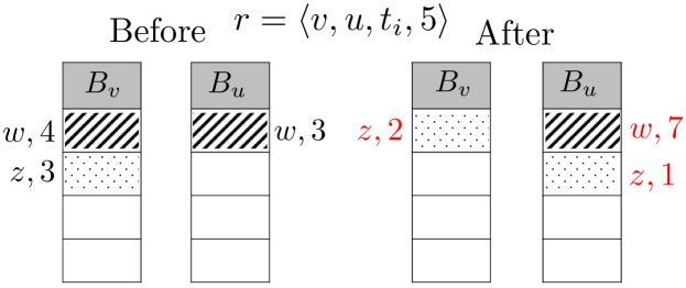
Figure 1. Example of quantity transfer (FIFO policy)

Objective and Methodology In this paper, we study a provenance problem in TINs. Our goal is to track the origin (source) of the quantities that are accumulated at the vertices over time. To do so, we first need to specify how data are transferred from one vertex to another and when new quantities are generated. In general, we assume that each vertex $v$ has a buffer $B_{v}$ (e.g., bitcoin wallet) (Decker and Wattenhofer, 2013), wherein it accumulates all incoming quantities to $v$. Naturally, the buffer $B_{v}$ changes over time. Specifically, each interaction $r$ from a vertex $r.v$ to a vertex $r.u$ transfers $r.q$ units from $B_{r.v}$ to $B_{r.u}$ at time $r.t$. If $B_{r.v}$ has less than $q$ units by time $r.t$, then the difference must be generated at $r.v$ before being transferred to $r.u$. In a financial exchange network, generation of new quantities could mean that new assets are brought into the network from external sources (e.g., a user buys bitcoins by paying USD). In a road network, new quantities are cars entering the network from a given location.

We propose solutions that proactively create and propagate lightweight provenance information in the TIN for the generated quantities, as they are transferred through the network. This way, we can obtain the origins of the quantities at vertices at any time. We define and study alternative information propagation models that may apply to different application scenarios. Specifically, consider an interaction $r$ from a vertex $r.v$ to a vertex $r.u$, which transfers $r.q$ units and assume that $r.q$ is smaller than the current number of units in buffer $B_{r.v}$. In this case, $r.q$ units should be selected from the buffer to be transferred, based on a policy. The selection policy could prioritize quantities based on the time they were first generated at their origins, or on the order they were added to $B_{r.v}$, or could select quantities proportionally based on their origins. For instance, Figure 1 shows the buffers $B_{v}$ and $B_{u}$ of two vertices $v$ and $u$ before and after an interaction $\langle v,u,t_{i},5\rangle$. The quantities in the buffers are organized as a FIFO queue based on their origins (e.g., $B_{v}$ contains 4 and 3 units originating from vertex $w$ and vertex $z$, respectively). Based on the FIFO policy, all 4 units from $w$ are selected to be transferred plus 1 unit from $z$. For each of the selection policies that we consider, we propose provenance update mechanisms and study efficient and space-economic algorithms for annotation propagation.

Previous Work To our knowledge, there is no previous work that studies data provenance in TINs. Within our framework, we define and use data transfer models for TINs, which are based on data relay, i.e., data units that move in the network are not cloned or deleted. On the other hand, most previous works define and study information diffusion models (Richardson and Domingos, 2002; Kumar and Calders, 2017), where data items (e.g., news, rumors, etc.) are spread in the network and the main objective is to identify the vertices of maximal influence in the network (Kempe et al., 2003), targeting applications such as viral marketing. Hence, previous efforts on provenance tracing for social networks (Barbier et al., 2013; Taxidou et al., 2015) are based on different information propagation models compared to our work.

Data provenance is a core concept in database query evaluation (Buneman et al., 2001) and workflow graphs (Chapman et al., 2008; Psallidas and Wu, 2018b). The main motivation is tracing the raw data which contribute to a query output. Data provenance finds use in most types of networks (e.g., threat identification in communication networks (Han et al., 2020)). Data provenance can be categorized into: where, how and why provenance (Cheney et al., 2009). Where-provenance identifies the raw data which contribute to some output, why-provenance identifies the sources (e.g., tuples) that influenced the output (Lee et al., 2020, 2018, 2019), and how-provenance explains how the input sources contribute to the output. Our work focuses on solving both the where- and why-provenance problem in TINs, i.e., find the vertices that contribute to each vertex over time. We also extend our solution to support how-provenance, i.e., capture the paths that have been followed by quantities. Our solutions can shed light to the reasons behind the accumulation of a quantity at a given vertex. Key differences to previous work on data provenance are: (i) in our problem, any vertex of the graph can be the origin of a quantity and any vertex can also be the destination of a propagated quantity; and (ii) we support the maintenance of provenance information in real-time, as new interactions take place in a streaming fashion.

Applications Solving our provenance problem in TINs finds application in various domains. In financial networks, tracking the origin of financial units that move between accounts can help in analyzing their relationships. For example, we can identify the accounts that (indirectly) contributed the most in financing a suspicious account. We can also characterize accounts based on whether they receive funds from numerous or few sources, or identify groups of users that finance other groups of users. Another example of a TIN is a communication network, where messages are transferred between vertices and there is a need to trace the origins of malicious messages that reach a vertex. Tracing the origin of such messages can be hard due to IP spoofing (Morris, 1985) and there is a need for specialized techniques (Savage et al., [n.d.]). Similarly, in transportation networks (e.g., flight networks or road networks) studying the provenance of problems (e.g., traffic, delays, etc.) may help in finding and alleviating the reasons behind them. As a provenance data analysis example, consider one of the TINs used in our experiments, which captures the transfers of passengers by taxi between NYC districts on 2019.01.01. Figure 2 shows the number of passengers that are accumulated in East Village from other districts. After each transfer, we can analyze the provenance distribution of passengers (shown as pie charts). This can be used to analyze the demographics of visitors over time (e.g., for location-aware marketing).

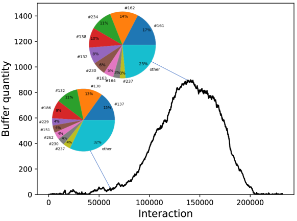
Figure 2. Buffered quantities at vertex #79 (East Village) after each interaction in Taxis Network

Contributions and outline Our main contribution is the formulation of a provenance tracking problem in temporal interaction networks with important applications. We define different selection policies for the propagation of quantities and the corresponding annotation generation and propagation algorithms. We analyze the space and time complexity of the provenance mechanism that we propose for each selection policy and find that the proportional propagation policy is infeasible for large graphs because its space complexity is quadratic to the number of vertices $|V|$ and each interaction bears a $O(|V|)$ computational cost.

We propose restricted, but practical versions of provenance tracking under the proportional propagation policy. Our selective provenance tracking approach maintains provenance data only from a designated subset of $k$ vertices, which are of interest to the analyst, reducing the space complexity to $O(k\cdot|V|)$ and the time complexity to $O(k)$ per interaction. The grouped provenance tracking approach tracks provenance from groups of vertices instead of individual vertices (e.g., categories of financial entities or accounts). Again, the space and time complexity is reduced to $O(k\cdot|V|)$ and $O(k)$ per interaction, respectively, if $k$ is the number of groups. We also propose two techniques that limit the scope of provenance tracking from all (individual) vertices. The first approach limits provenance tracking up to a certain time in the past from the current interaction (i.e., a time-window approach). The second approach allocates a provenance budget to each vertex. Both techniques save resources, while providing some guarantees with respect to either time or importance of the tracked provenance information.

We extend our propagation algorithms for provenance annotations to capture not only the origins of the generated data, but the routes (i.e., the paths) that they travelled along in the graph until they reached their destinations.

We experimentally evaluate the runtime and memory requirements of our methods on five real TINs with different characteristics. Our results show the scalability and limitations of the different selection policies and the corresponding propagation algorithms for provenance data.

The rest of the paper is organized as follows. Section 2 reviews related work on data provenance and TINs. In Section 3, we formally define the provenance problem in TINs. Section 4 presents the different information propagation policies and the corresponding provenance tracking algorithms. In Section 5, we discuss scaleable techniques for provenance tracking under the proportional propagation policy. In Section 6, we show how to track the paths of the propagated quantities in the TINs from their origin. Section 7 presents our experimental evaluation. Finally, Section 8 concludes the paper with a discussion about future work.

2. Related Work

There has been a lot of research in data provenance over the years (Rupprecht et al., 2020; Barbier et al., 2013; Chothia et al., 2016; de Paula et al., 2013; Lee et al., 2020; Psallidas and Wu, 2018a; Parulian et al., 2021; Namaki et al., 2020). However, we are the first to study the problem of tracking the origin of quantities that flow in temporal interaction networks. In this section, we summarize representative works in temporal interaction networks and provenance tracking.

2.1. Temporal Interaction Networks

Temporal interaction networks (TINs) capture the exchange of quantities between entities over time and they have been studied extensively in the literature (Akrida et al., 2017; Li et al., 2017; Masuda and Holme, 2013). For instance, Kosyfaki et al. (Kosyfaki et al., 2019) studied the problem of finding recurrent flow path patterns in a TIN, during time windows of specific length. Pattern detection in TINs with an application in social network analysis was also studied in (Züfle et al., 2018; Belth et al., [n.d.]). A related problem is how to measure the total quantity that flows between two specific vertices in a TIN (Akrida et al., 2017; Kosyfaki et al., 2021). Zhou et al. (Zhou et al., 2020) study the problem of dynamically synthesizing realistic TINs by learning from log data. Provenance in TINs can reveal data that can be combined with the structural and flow information of a TIN in order to make pattern detection and graph synthesis more accurate or explain the mining results.

2.2. Theory and Applications in Provenance

Buneman et al. (Buneman et al., 2001) were the first who defined and studied the problem of data provenance in database systems. The goal of why-provenance (a.k.a. lineage) is to explain the existence of a tuple $t$ in a query result by finding the tuples present in the input that contributed to the production of $t$. Where-provenance finds the exact attribute values from the input which were copied or transformed to produce $t$. An annotation mechanism for where-provenance was proposed in (Buneman et al., 2002) and implemented in DBNotes (Bhagwat et al., 2004). As query operators (select, project, join, etc.) are executed, annotations are propagated to eventually reach the query output tuples. Annotation propagation depends on the way the query is written/evaluated. Geerts et al. (Geerts et al., 2006) introduced another annotation-based model for the manipulation and querying of both data and provenance, which allows annotations on sets of values and for effectively querying how they are associated. The focus is on scientific database curation, where data from possibly multiple sources are integrated and annotations are used to witness the association between the base data that produced a curated tuple.

Although our solutions share some similarities to provenance approaches for database systems, there are important differences in the data and the propagation models. First, the TIN graphs that we examine are very large (as opposed to small query graphs) and we track provenance for any vertex in them (i.e., we do not distinguish between input and output vertices). Second, the data transfer model between vertices in TINs is very different compared to data transfer in query graphs. Third, interactions can happen in any order in our TINs, as opposed to query graphs, where edges have a specific order (query graphs are typically DAGs).

Data Provenance has also been studied in social networks (Barbier et al., 2013). An important application is to detect where from a rumor has started before spreading through the internet. Gundecha et al. (Gundecha et al., 2013) represent social networks as directed graphs and try to recover paths to find out how information spread through the network by isolating important nodes (less than 1%). The importance of the nodes is based on their centrality. Taxidou et al. (Taxidou et al., 2015) studied provenance within an information diffusion model, based on the W3C Provenance Data Model. A related problem in social networks is information propagation and diffusion. Domingos and Richardson (Domingos and Richardson, 2001) were the first who studied techniques for viral marketing to influence social network users. Kempe et al. (Kempe et al., 2003) solved the problem of selecting the most influential nodes by proposing a linear model, where the network is represented as a directed graph and vertices are categorized as active and inactive based on their neighbors. These approaches are not applicable to TINs, because, in social networks, information is copied and diffused, whereas in TINs data are moved (i.e., not copied) from one vertex to another. This key difference makes the provenance problem in TINs unique compared to related problems in previous work.

Savage et al. (Savage et al., [n.d.]) propose a stochastic packet marking mechanism that can be used for probabilistic tracing back packet-flooding attacks in the Internet. The problem setup is quite different than ours, since we target a more generic provenance problem in TINs where information is propagated based on various different models that may not permit backtracing. Moreover, we aim at exact provenance tracking wherever possible.

2.3. Provenance Systems

Over the years, a number of systems for provenance tracking have been developed, mainly to serve the need of efficiently storing and managing the annotation data. Chapman et al. (Chapman et al., 2008) propose a factorization technique, which identifies and unifies common query evaluation subtrees for reducing the provenance storage requirements. Heinis and Alonso (Heinis and Alonso, 2008) represent workflow provenance mechanisms as DAGs and compress DAGs with common nodes, in order to save space.

Several systems (Agrawal et al., 2006; Green et al., 2010) have been developed to support the answering of data provenance questions, where the objective is to find how a data element has appeared in the query result. Karvounarakis et al (Karvounarakis et al., 2010) developed ProQL, a query language which can be used to detect errors and side effects during the updates of a database. ProQL takes advantage of the graph representation and path expressions to simplify operations involving traversal and projection on the provenance graph. Titian (Interlandi et al., 2015) adds provenance support to Spark, aiming at identifying errors during query evaluation.

Glavic et al. (Glavic et al., 2013) present a system for provenance tracking in data stream management systems (DSMS). They propose an operator instrumentation model, which annotates data tuples that are generated or propagated by the streaming operators with their provenance. They also propose an alternative approach (called replay lazy), which uses the original operators and, whenever provenance information is needed, the approach replays query processing on the relevant inputs through a instrumented copy of the network (hence, data processing and provenance computation are decoupled). We also propose space-economic models for tracking provenance. However, our input graphs (TINs) are larger and different than DSMS graphs and our propagation models consider the transfer of quantities between vertices as a result of a stream of interactions.

Provenance has also been studied in blockchain systems especially after the huge success of Bitcoin. In (Ruan et al., 2019), a secure and efficient system called LineageChain is implemented on top of Hyperledger, for capturing the provenance during contract execution and safely storing it in a Merkle tree.

3. Definitions

In this section, we formally define the temporal interaction network (TIN) on which our problem applies. Then, we present the data propagation model, which determines the origins of the quantities which are transferred in the network. Finally, we define the provenance problem that we study in this paper. Table 1 summarizes the notation used frequently in the paper.

Definition 0 (Temporal Interaction Network).

A temporal interaction network (TIN) is a directed graph $G(V,E,R)$. Each edge $(v,u)$ in $E$ captures the history of interactions from vertex $v$ to vertex $u$. $R$ denotes the set of interactions on all edges of $E$. Each interaction $r\in R$ is characterized by a quadruple $\langle r.s,r.d,r.t,r.q\rangle$, where $r.s\in V$ ($r.d\in V$) is the source (destination) vertex of the interaction, $r.t\in{\rm I\!R}^{+}$ is the time when the interaction took place and $r.q\in{\rm I\!R}^{+}$ is the transferred quantity from vertex $r.s$ to $r.d$, due to interaction $r$.

$r.s$ $r.d$ $r.t$ $r.q$ $v_{1}$ $v_{2}$ 1 3 $v_{2}$ $v_{0}$ 3 5 $v_{0}$ $v_{1}$ 4 3 $v_{1}$ $v_{2}$ 5 7 $v_{2}$ $v_{1}$ 7 2 $v_{2}$ $v_{0}$ 8 1

(a) Interactions

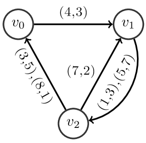
(b) TIN

Figure 3. A set of interactions and the corresponding TIN

Figure 3 shows the set $R$ of interactions in a TIN and the corresponding graph. For example, sequence $\{(1,3),(5,7)\}$ on edge $(v_{1},v_{2})$ means that $v_{1}$ transferred to $v_{2}$ a quantity of $3$ units at time $1$ and then $7$ units at time $5$. The corresponding interactions in $R$ are $\langle v_{1},v_{2},1,3\rangle$ and $\langle v_{1},v_{2},5,7\rangle$.

Table 1. Table of notations

Notation	Description
$G(V,E,R)$	TIN (vertices, edges, interactions)
$r.s$	source vertex of interaction $r\in R$
$r.d$	destination vertex of interaction $r\in R$
$r.t$	time when interaction $r\in R$ took place
$r.q$	transferred quantity during interaction $r\in R$
$B_{v}$, $|B_{v}|$	buffer of vertex $v$, total quantity in $B_{v}$
$O(t,B_{v})$	origin (provenance) data for the quantity at $B_{v}$ by time $t$
$(\tau.o,\tau.q)$	quantity $\tau.q$ originating from $\tau.o$ in $O(t,B_{v})$
$\mathbf{p}_{v}$	provenance vector of a vertex $v\in V$

We consider all interactions $R$ in the TIN in order of time and assume that throughout the timeline, each vertex $v\in V$ has a buffer $B_{v}$, which stores the total quantity that has flown into $v$ but has not been transferred yet to another vertex via an outgoing interaction from $v$. We use $|B_{v}|$ to denote the quantity buffered at $B_{v}$.

As an effect of an interaction $\langle r.s,r.d,r.t,r.q\rangle$, vertex $r.s$ transfers a quantity of $r.q$ to vertex $r.d$. Quantity $r.q$ (or part of it) could be data that have been accumulated at vertex $r.s$ by time $r.t$, or $r.q$ could (partially) be generated at $r.s$. More specifically, we distinguish between two cases:

• $|B_{r.s}|\leq r.q$. In this case, all units from $B_{r.s}$ are transferred to $B_{r.d}$ due to the interaction. In addition, $r.q-|B_{r.s}|$ units are generated by the source vertex $r.s$ and transferred to $B_{r.d}$. Hence, $|B_{r.s}|$ becomes 0 and $|B_{r.d}|$ is increased by $r.q$.

• $|B_{r.s}|>r.q$. In this case, $r.q$ units are selected from $B_{r.s}$ to be transferred to $B_{r.d}$. Hence, $|B_{r.s}|$ is decreased by $r.q$ and $|B_{r.d}|$ is increased by $r.q$. The selection policy may determine the routes of the quantities in the network and may affect the result of provenance tracking.

1:TIN $G(V,E,R)$

2:for each $v\in V$ do

3:    $|B_{v}|=0$ $\triangleright$ Initialize buffers

4:end for

5:for each interaction $r\in R$ in order of time do

6:    $q=\min\{r.q,B_{r.s}\}$ $\triangleright$ relayed quantity from $B_{r.s}$

7:    $|B_{r.s}|=|B_{r.s}|-q$ $\triangleright$ decrease by $q$

8:    $|B_{r.d}|=|B_{r.d}|+r.q$ $\triangleright$ increase by $r.q$, $r.q$$-$$q$ newborn units

9:end for

Algorithm 1 Propagation algorithm in a TIN

Algorithm 1 is a pseudocode of the data propagation procedure. Interactions in $R$ are processed in order of time. For each interaction $r\in R$, we first determine the relayed quantity $q$ from the buffer of the source vertex $r.s$ (Line 6). This quantity cannot exceed the currently buffered quantity $|B_{r.s}|$ at $r.s$. Line 7 decreases $B_{r.s}$, accordingly. The target node’s buffer $B_{r.d}$ is increased by $r.q$ (Line 8). If $r.q>q$, a new quantity $r.q-q$ is born by the source vertex $r.s$ to be transferred to $B_{r.d}$ as part of $r.q$.

Table 2 shows the changes in the buffers of the three vertices in the example TIN (Figure 3), during the application of Algorithm 1. The values in the parentheses are the newborn quantities at $r.s$, which are transferred to $r.d$. In the beginning, all buffers are empty, hence, as a result of the first interaction, 3 quantity units are born at vertex $v_{1}$ and transferred to $v_{2}$, but no previously born quantity is relayed from $B_{v_{1}}$ to $B_{v_{2}}$. At the second interaction, 3 units move from $B_{v_{2}}$ to $B_{v_{0}}$ and 2 newborn units at $v_{2}$ are also transferred to $B_{v_{0}}$. At the third interaction, 3 units are selected to be transferred from $B_{v_{0}}$ to $B_{v_{1}}$ and no new units are generated because the $B_{v_{0}}$ had more units than $r.q=3$ before the interaction.

Table 2. Changes at buffers at each Interaction

$r.s$	$r.d$	$r.t$	$r.q$	$|B_{v_{0}}|$	$|B_{v_{1}}|$	$|B_{v_{2}}|$
$v_{1}$	$v_{2}$	1	3	0	0	3 (3)
$v_{2}$	$v_{0}$	3	5	5 (2)	0	0
$v_{0}$	$v_{1}$	4	3	2	3	0
$v_{1}$	$v_{2}$	5	7	2	0	7 (4)
$v_{2}$	$v_{1}$	7	2	2	2	5
$v_{2}$	$v_{0}$	8	1	3	2	4

Definition 3.2 formally defines the provenance problem that we study in this paper.

Definition 0 (Provenance Problem).

Given a TIN $G(V,E,R)$, at any time moment $t$ and at any vertex $v\in V$ determine the origin(s) $O(t,B_{v})$ of the total quantity accumulated at buffer $B_{v}$ by time $t$. $O(t,B_{v})$ is a set of $(\tau.o,\tau.q)$ tuples $\tau$, such that each quantity $\tau.q$ was generated by vertex $\tau.o$ and $\sum_{\tau\in O(t,B_{v})}\tau.q=|B_{v}|$.

At any time $t$, during Algorithm 1, the objective is to be able to identify the origin vertices which have generated the quantities that have been accumulated at buffer $B_{v}$, for any vertex $v$. Hence, the problem is to divide the buffer $B_{v}$ into a set of $(\tau.o,\tau.q)$ (origin-quantity) pairs, such that each quantity $\tau.q$ is generated by the corresponding vertex $\tau.o$. A data analyst can then know how the total quantity buffered at $v$ has been composed.

4. Selection Policies and Provenance

For each interaction $r\in R$, the selection policy in the case where $|B_{r.s}|>r.q$ determines the provenance of the quantities that are accumulated at any vertex $v$ (and transferred from $v$) throughout the timeline. Selection does make a difference because the quantities in a buffer $B_{r.s}$ may originate from different vertices. We present possible selection policies that (i) are based on the time quantities are generated, (ii) are based on the order they are received by the vertex $r.s$ or (iii) choose quantities proportionally based on their origins. For each policy, we present annotation mechanisms that can be used to trace the provenance of the quantities accumulated at the vertices of the TIN. We also discuss applications where these selection policies may apply.

4.1. Selection based on generation time

The first selection policy is based on the time when the candidate quantities to be transferred are generated. Priority in the selection can be given to the oldest quantities or the most recently generated ones depending on the application. We will first discuss the least recently born selection policy. To implement this approach, any generated quantity should be marked with the vertex $v$ that generates it and the timestamp $t$ when it is generated. Hence, during the course of the algorithm, each buffer $B_{v}$ is modeled and managed as a set of $(o,t,q)$ triples, where $o$ is the origin of (i.e., the vertex which bore) quantity $q$ and $t$ is the time of birth of $q$. The total quantity $|B_{v}|$ accumulated at buffer $B_{v}$ is the sum of all $q$ values in the triples that constitute $B_{v}$. As a result of an interaction $r$, if $|B_{r.s}|>r.q$, the triples in $B_{r.s}$ with the smallest timestamps whose quantities sum up to $r.q$ are selected and transferred to $B_{r.d}$. The last triple may be partially transferred in order for the transferred quantity to be exactly $r.q$. The triples in each buffer $B_{v}$ are organized in a min-heap in order to facilitate the selection.

Algorithm 2 describes the whole process. For the current interaction $r\in R$ in order of time, we maintain in variable $resq$ the residue quantity, which has yet to be transferred from $r.s$ to $r.d$. Initially, $resq=r.q$. While $q>0$ and $B_{r.s}$ is not empty, we locate the least recently born triple $\tau$ in $B_{r.s}$ (with the help of the min-heap). If $\tau.q>q$, this means that we should transfer part of the quantity in the triple to $B_{r.d}$, hence, we split $\tau$, by keeping it in $B_{r.s}$ and reducing $\tau.q$ by $q$ and initializing a new triple $\tau^{\prime}$ with the same origin and birthtime as $\tau$ and quantity $q$. The new triple is added to $B_{r.d}$. If $\tau.q\leq q$, we transfer the entire triple $\tau$ from $B_{r.a}$ to $B_{r.d}$. If $B_{r.s}$ becomes empty and $resq>0$, then this means that it was $|B_{r.s}|<r.q$ in the beginning, so we should generate a newborn triple $\tau^{\prime}$ with the residue quantity $resq$, having as origin vertex $r.s$ and marked to be generated at time $r.t$.

1:TIN $G(V,E,R)$

2:for each $v\in V$ do

3:    $B_{v}=\emptyset$; $|B_{v}|=0$ $\triangleright$ Initialize buffers

4:end for

5:for each interaction $r\in R$ in order of time do

6:    $resq=r.q$ $\triangleright$ residue quantity to be transferred

7:    while $resq>0$ and $|B_{r.s}|>0$ do

8:         $\tau=$ least recent triple in $B_{r.s}$ $\triangleright$ top element in heap $B_{r.s}$

9:         if $\tau.q>resq$ then $\triangleright$ split $\tau$

10:             $\tau^{\prime}.o=\tau.o$; $\tau^{\prime}.t=\tau.t$; $\tau^{\prime}.q=resq$; $\triangleright$ new triple

11:             add $\tau^{\prime}$ to $B_{r.d}$;

12:             $\tau.q=\tau.q-r.q$;$\triangleright$ update $\tau$

13:             $resq=0$; $\triangleright$ transfers completed

14:         else

15:             remove $\tau$ from $B_{r.s}$ and add it to $B_{r.d}$;

16:             $resq=resq-\tau.q$ $\triangleright$ update residue quantity

17:         end if

18:    end while

19:    if $resq>0$ then $\triangleright$ newborn quantity and triple

20:         $\tau^{\prime}.o=r.s$; $\tau^{\prime}.t=r.t$; $\tau^{\prime}.q=resq$;

21:         add $\tau^{\prime}$ to $B_{r.d}$;

22:    end if

23:end for

Algorithm 2 Least-recently born selection model

Table 3 shows the changes in the buffers of the vertices (shown as sets here, but organized as min-heaps with their middle element $t$ as key) after each interaction of our running example. Note that the quantities in the buffers are broken based on their origins and times of birth.

Table 3. Changes at buffers (oldest-first policy)

$r.s$	$r.d$	$r.t$	$r.q$	$B_{v_{0}}$	$B_{v_{1}}$	$B_{v_{2}}$
$v_{1}$	$v_{2}$	1	3	$\emptyset$	$\emptyset$	{(1,1,3)}
$v_{2}$	$v_{0}$	3	5	{(1,1,3),(2,3,2)}	$\emptyset$	$\emptyset$
$v_{0}$	$v_{1}$	4	3	{(2,3,2)}	{(1,1,3)}	$\emptyset$
$v_{1}$	$v_{2}$	5	7	{(2,3,2)}	$\emptyset$	{(1,1,3),(1,5,4)}
$v_{2}$	$v_{1}$	7	2	{(2,3,2)}	{(1,1,2)}	{(1,1,1),(1,5,4)}
$v_{2}$	$v_{0}$	8	1	{(1,1,1),(2,3,2)}	{(1,1,2)}	{(1,5,4)}

By running Algorithm 2, we can have at any time $t$ the set of vertices that contribute to a vertex $v$ by time $t$ and the corresponding quantities (i.e., the solution to Problem 3.2). In other words, the heap contents for each vertex $v$ at time $t$ corresponds to $O(t,B_{v})$. Finally, to implement the most recently born selection policy, we should change Line 8 of Algorithm 2 to “$\tau=$ most recent triple in $B_{r.s}$” and organize each buffer as a max-heap (instead of a min-heap).

Application The least recently born policy is applicable when the generated quantities lose their value over time (or even expire), which means that the vertices prefer to keep the most recently generated data. On the other hand, the most recently born policy is relevant to applications, where quantities have antiquity value, i.e., they become more valuable as time passes by.

Complexity Analysis In the worst case, each interaction $r$ increases the total number of triples by one (i.e., by splitting the last transferred triple or by generating a new triple), hence, the space complexity of the entire process is $O(|R|)$. In terms of time, each interaction accesses in the worst case the entire set of triples at vertex $r.s$. This set is $O(|R|)$ in the worst case, but we expect it to be $O(|R|/|V|)$; for each triple in the set, we update two priority queues in the worst case (i.e, by triple transfers) at an expected cost of $O(\log|R|/|V|)$. Hence, the overall expected cost (assuming an even distribution of triples) is $O(|R|\cdot|R|/|V|\cdot\log|R|/|V|)=O(|R|^{2}/|V|\log|R|/|V|)$.

4.2. Selection based on order of receipt

Another policy would be to select the transferred quantities in order of their receipt. Specifically, the quantities at each buffer $B_{v}$ are modeled and managed as a set of $(o,q)$ pairs, where $o$ is the vertex which generated $q$. These pairs are organized based on the order by which they have been inserted to $B_{v}$. If, for the current transaction $r$, $|B_{r.s}|>r.q$, the last (or the first) quantities in $B_{r.s}$ which sum up to $r.q$ are selected and added to $B_{r.d}$ in their selection order. To implement this policy, each buffer is implemented as a FIFO (or LIFO) queue, hence, it is not necessary to keep track of the transfer-time timestamps. The algorithm is identical to Algorithm 2, except that Line 8 becomes “least recently added triple in $B_{r.s}$” in the FIFO policy and “most recently added triple in $B_{r.s}$” in the LIFO policy. Table 4 shows the changes in the buffers after each interaction when the LIFO policy is applied.

Table 4. Changes at buffers (LIFO policy)

$r.s$	$r.d$	$r.t$	$r.q$	$B_{v_{0}}$	$B_{v_{1}}$	$B_{v_{2}}$
$v_{1}$	$v_{2}$	1	3	$\emptyset$	$\emptyset$	{(1,3)}
$v_{2}$	$v_{0}$	3	5	{(1,3),(2,2)}	$\emptyset$	$\emptyset$
$v_{0}$	$v_{1}$	4	3	{(1,2)}	{(1,1),(2,2)}	$\emptyset$
$v_{1}$	$v_{2}$	5	7	{(1,2)}	$\emptyset$	{(1,1),(2,2),(1,4)}
$v_{2}$	$v_{1}$	7	2	{(1,2)}	{(1,2)}	{(1,1),(2,2),(1,2)}
$v_{2}$	$v_{0}$	8	1	{(1,2),(1,1)}	{(1,2)}	{(1,1),(2,2),(1,1)}

Application The FIFO policy is used in applications where the buffers are naturally implemented as FIFO queues (pipelines, traffic networks). The LIFO policy applies when the accumulated quantities are organized in a stack (e.g., cash registers, wallets) before being transferred.

Complexity Analysis The space complexity is $O(|R|)$, same as that of generation time selection policies (Sec. 4.1), because the only change is that we replace the heap by a FIFO queue (or a stack). This replacement changes the access and update costs from $O(\log|R|/|V|)$ to $O(1)$. Hence, the overall expected cost is reduced from $O(|R|^{2}/|V|\log|R|/|V|)$ to $O(|R|^{2}/|V|)$.

4.3. Proportional selection

The proportional selection policy, for the case where $|B_{r.s}|>r.q$, chooses the relayed quantity from $r.s$ to $r.d$ proportionally from the vertices that have contributed to $B_{r.s}$, based on their contribution.

Formally, for each vertex $v\in V$, we define a $|V|$-length vector $\mathbf{p}_{v}$, which captures the provenance of the quantity currently in its buffer $B_{v}$. The $i$-th value of $\mathbf{p}_{v}$ is the quantity fragment in $B_{v}$ which originates from the $i$-th vertex of the TIN $G$. Hence, the sum of quantities in $\mathbf{p}_{v}$ equals the total quantity $|B_{v}|$ in $B_{v}$. Initially, all values of $\mathbf{p}_{v}$ are 0.

Algorithm 3 shows how the provenance vectors are updated after each interaction $r$. We distinguish between two cases. The first one is when $r.q\geq|B_{r.s}|$, i.e., the quantity $r.q$ to be transferred by the current interaction is greater than or equal to the buffered quantity $|B_{r.s}|$ at the source buffer. In this case, the entire buffered quantity in $B_{r.s}$ is relayed to $B_{r.d}$. Hence, vector $\mathbf{p}_{r.s}$ is added to $\mathbf{p}_{r.d}$ (symbol $\oplus$ denotes vector-wise addition). If $r.q$ is strictly greater than $|B_{r.s}|$, a newborn quantity $r.q-|B_{r.s}|$ at $r.s$ is added to $B_{r.d}$, hence, we should add the corresponding provenance information to the $r.s$-th element of $\mathbf{p}_{r.d}$ (Line 7). This is denoted by the addition of vector $\mathbf{e}_{r.s,(r.q-B_{r.s})}$, where $\mathbf{e}_{v,x}$ denotes a vector with all $0$’s except having value $x$ at position $v$. The second case is when $r.q<|B_{r.s}|$. In this case, the quantity $r.q$ which is transferred from $r.s$ to $r.d$ is chosen proportionally. Specifically, if vertex $r.s$ has in its buffer $B_{r.s}$ a quantity $q$ which was born by the $i$-th vertex, then a quantity $q\cdot\frac{r.q}{|B_{r.s}|}$ should be transferred from the $i$-th position of $\mathbf{p}_{r.s}$ to the $i$-th position of $\mathbf{p}_{r.d}$. This translates into the vector-wise operations at Lines 10 and 11 of Algorithm 3. Table 5 shows the changes in the buffer vectors after each interaction when proportional selection is applied.

1:TIN $G(V,E,R)$

2:for each $v\in V$ do

3:    $|B_{v}|=0$; $\mathbf{p}_{v}=\mathbf{0}$; $\triangleright$ Initialize buffers and vectors

4:end for

5:for each interaction $r\in R$ in order of time do

6:    if $r.q\geq|B_{r.s}|$ then

7:         $\mathbf{p}_{r.d}=\mathbf{p}_{r.d}\oplus\mathbf{p}_{r.s}\oplus\mathbf{e}_{r.s,(r.q-B_{r.s})}$; $\mathbf{p}_{r.s}=\mathbf{0}$;

8:         $|B_{r.d}|=|B_{r.d}|+r.q$; $|B_{r.s}|=0$;

9:    else$\triangleright$ $r.q<|B_{r.s}|$

10:         $\mathbf{p}_{r.d}=\mathbf{p}_{r.d}\oplus(r.q/|B_{r.s}|)\mathbf{p}_{r.s}$; $B_{r.d}=B_{r.d}+r.q$;

11:         $\mathbf{p}_{r.s}=\mathbf{p}_{r.s}\ominus(r.q/|B_{r.s}|)\mathbf{p}_{r.s}$; $B_{r.s}=B_{r.s}-r.q$;

12:    end if

13:end for

Algorithm 3 Proportional selection model

Table 5. Changes at buffers (proportional selection)

$r.s$	$r.d$	$r.t$	$r.q$	$\mathbf{p}_{v_{0}}$	$\mathbf{p}_{v_{1}}$	$\mathbf{p}_{v_{2}}$
$v_{1}$	$v_{2}$	1	3	$[0,0,0]$	$[0,0,0]$	$[0,3,0]$
$v_{2}$	$v_{0}$	3	5	$[0,3,2]$	$[0,0,0]$	$[0,0,0]$
$v_{0}$	$v_{1}$	4	3	$[0,1.2,0.8]$	$[0,1.8,1.2]$	$[0,0,0]$
$v_{1}$	$v_{2}$	5	7	$[0,1.2,0.8]$	$[0,0,0]$	$[0,5.8,1.2]$
$v_{2}$	$v_{1}$	7	2	$[0,1.2,0.8]$	$[0,1.66,0.34]$	$[0,4.14,0.86]$
$v_{2}$	$v_{0}$	8	1	$[0,2.03,0.97]$	$[0,1.66,0.34]$	$[0,3.31,0.69]$

Application Proportional selection makes sense in applications where the quantities are naturally mixed in the buffers. This includes cases when the transferred data are liquids (e.g., buffers are oil tanks) or indistinguishable financial units in accounts (i.e., balances in bank accounts, capital stocks in digital portfolios). In such cases, it is reasonable to consider that the origins of the buffered quantities contribute proportionally to a transfer.

Complexity Analysis The provenance vectors $\mathbf{p}_{v}$ raise the space requirements of this model to $O(|V|^{2})$, i.e., we need a $|V|$-length vector for each vertex. In the next section, we will explore a number of directions in order to reduce the space requirements and make proportional provenance tracking feasible for large graphs with millions of vertices. The time complexity is also high, because we need one or two vector-wise operations per interaction, which accumulates to a $O(|R|\cdot|V|)$ cost. In our implementation, we exploit SIMD instructions (Polychroniou et al., 2015) to reduce the cost of vector-wise operations.

Sparse vector representations In sparse graphs, each vertex $v$ may receive quantities originating from a small subset of vertices in practice. To save space, instead of storing each space-demanding vector $\mathbf{p}_{v}$ explicitly, we can represent it by an ordered list of $(u,q)$ pairs, for each vertex $u$ contributing a quantity $q>0$ in the buffer $B_{v}$. For example, after the temporally first interaction in our running example, instead of storing $\mathbf{p}_{v_{2}}$ as $[0,3,0]$, we store it as $[(v_{1},3)]$, implying that $v_{2}$ received its 3 units from $v_{1}$. The vector update operations of Algorithm 3 can be replaced by merging the ordered lists of the corresponding sparse vector representations. This way, the space requirements are reduced from $O(|V|^{2}|)$ to $O(|V|\cdot\ell)$, where $\ell$ is the average length of the list representations of the vectors. The time complexity is reduced to $O(|R|\cdot\ell)$, accordingly. Still, as we show experimentally, in Section 7, $\ell$ can grow too large and we may not be able to accommodate the lists in memory, after a long sequence of interactions.

5. Scalable Proportional Provenance

Proportional provenance tracking (Section 4.3) has high space and time complexity compared to the models based on generation time (Section 4.1) or receipt order (Section 4.2). We investigate a number of techniques that reduce the space requirements and constitute proportional provenance feasible even on very large graphs.

5.1. Selective provenance tracking

In many applications, we may not have to track provenance from all vertices in the graph, but from a selected subset thereof. For example, in a financial network, we could limit our focus to a specific set of entities, suspected to be involved in illegal activities. Or, we may select the $k$ vertices that generate the largest total quantities. Hence, we can limit the size of the provenance tracking vectors $\mathbf{p}_{v}$ to include only a given subset of vertices having limited size $k$.

Specifically, for each vertex $v\in V$, we maintain a vector $\mathbf{p}_{v}$ of size $k+1$, where the first $k$ positions correspond to the vertices of interest and the last position represents the rest of the vertices. Algorithm 3 can now directly be applied, after the following change: if any of the source vertex $r.s$ or the destination $r.d$ is not in the set of the $k$ vertices of interest, we update the $(k+1)$-th position, which accumulates the sum of quantities from all vertices except the selected ones. This version of proportional selection algorithm has reduced space and time complexity compared to Algorithm 3. Specifically, its space requirements are $O(k\cdot|V|)$ and its time complexity is $O(k\cdot|R|)$.

5.2. Grouped provenance tracking

In practice, tracking provenance from individual vertices could provide too many details which might be hard to interpret. It might be more practical, to track provenance from groups of vertices. Hence, assuming that the vertices of the TIN have been divided into groups, we can replace the long $\mathbf{p}_{v}$ vectors by shorter vectors of length $m$, where $m$ is the number of groups. This means that, in the end, for each vertex $v$ we will have in $\mathbf{p}_{v}$ the total quantity in the buffer $B_{v}$ of $v$ which originates from each group. The grouping of vertices can be done in different ways depending on the application. For example, the values of one or more attributes that characterize the vertices in the application (e.g., gender, country) can be used for grouping. Network clustering algorithms (e.g., METIS (Karypis and Kumar, 1998)) or geographical clustering can be used to divide the vertices to groups.

Algorithm 3 can easily be adapted to operate on groups. The vertices involved at each interaction (i.e., $r.s$ and $r.d$) are mapped to group-ids and the corresponding positions are updated in the vector-wise operations. As in the case of selective provenance tracking (Section 5.1), the space and time complexity is reduced to $O(m\cdot|V|)$ and $O(m\cdot|R|)$, respectively.

5.3. Limiting the scope of provenance

If selective and grouped provenance is not an option, tracking proportional provenance in large graphs with millions of vertices could be infeasible. We investigate two techniques that limit the scope of provenance by either avoiding the tracking of quantities generated far in the past or setting a budget for provenance at each vertex. Our techniques are especially suitable for streaming data, where speed and feasibility are preferred over preciseness.

5.3.1. Windowing approach

Our first approach takes as input a parameter $W$, representing a window, which determines how far in the past we are interested in tracking provenance. Specifically, for each vertex $v$ we can guarantee finding the provenance of quantities that reach $v$, which where born up to $W$ interactions before. To achieve this, for each $v$, we initialize two sparse (i.e., list) provenance vector representations $\mathbf{p}^{odd}_{v}$ and $\mathbf{p}^{even}_{v}$. At each interaction, both lists are updated. However, whenever we reach an interaction $r$ whose order is a multiple of $W$, we reset either $\mathbf{p}^{odd}_{v}$ or $\mathbf{p}^{even}_{v}$ as follows. If the order of $r$ in the sequence $R$ of interactions is an odd multiple of $W$, for each vertex $v\in V$, we reset its provenance list $\mathbf{p}^{odd}_{v}$ by setting $\mathbf{p}^{odd}_{v}=[(\alpha,|B_{v}|)]$, where $\alpha$ is an artificial vertex, representing the entire set $V$ of vertices. This means that we assume that the entire quantity in $B_{v}$ has unknown provenance. If the order of $r$ is an even multiple of $W$, for all vertices $v$, we reset $\mathbf{p}^{even}_{v}$ by setting $\mathbf{p}^{even}_{v}=[(\alpha,|B_{v}|)]$. After any interaction $r$, we can track provenance for any vertex $v$ using whichever of $\mathbf{p}^{even}_{v}$ or $\mathbf{p}^{odd}_{v}$ was least recently reset. This guarantees that we can track the provenance of quantities born at least $W$ (and at most $2\cdot W$) interactions before. The space requirements (i.e., the total space required to store the provenance lists) are now controlled due to the provenance list resets.

Figure 4 illustrates how, for each vertex $v$, $\mathbf{p}^{odd}_{v}$ and $\mathbf{p}^{even}_{v}$ are updated and used. Assuming that $W=100$, until the $100$-th interaction, $\mathbf{p}^{odd}_{v}$ and $\mathbf{p}^{even}_{v}$ are identical and either of them can be used. Since $\mathbf{p}^{odd}_{v}$ is reset at the $100$-th interaction, between the $100$-th and the $200$-th interaction $\mathbf{p}^{even}_{v}$ is used to track the provenance of quantities which were generated since the first interaction. Similarly, between the $200$-th and the $300$-th interaction $\mathbf{p}^{odd}_{v}$ is used to track provenance up to the $100$-th interaction.

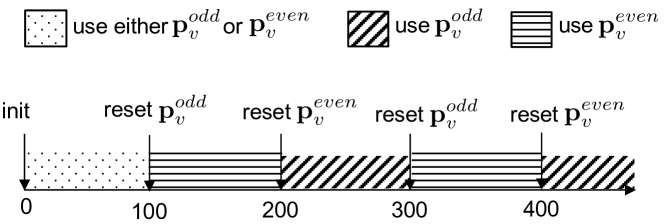
Figure 4. Windowing approach in provenance tracking

5.3.2. Budget-based provenance

Another approach which we can apply to control the memory requirements and make proportional provenance tracking feasible on large graphs is to allocate a maximum capacity $C$ (budget) to each vertex $v$ for its provenance list $\mathbf{p}_{v}$. Whenever we have to add new entries to $\mathbf{p}_{v}$, if the required capacity after the addition exceeds $C$, we select a certain fraction $f$ of entries to keep in $\mathbf{p}_{v}$. We remove the remaining entries and assume that the total quantity $Q$ which originates from them was born at an artificial vertex $\alpha$, modeling all vertices (i.e., unknown source). Hence, if $\mathbf{p}_{v}$ includes an $(\alpha,q)$ entry, the entry is updated to $(\alpha,q+Q)$; if not, a new entry $(\alpha,Q)$ is added to $\mathbf{p}_{v}$.

With this approach, the space requirements of proportional provenance tracking become $O(|V|\cdot C)$. The larger the value of $C$ the more accurate provenance tracking becomes. Parameter $f$ should be chosen such that the memory allocated at each vertex is not underutilized and, at the same time, shrinking does not happen very often. We suggest a value between $0.6$ and $0.8$. Finally, the selection of entries to keep when the budget $C$ is reached in $\mathbf{p}_{v}$ can be done using different criteria. For example, we can keep the entries with the largest quantities, or set a priority/importance order to vertices and keep provenance data for the most important ones.

As an example, assume that $\mathbf{p}_{v}=\{(v,1),(u,3),(w,2),(z,1)\}$ and let $C=5$. Let $\{(x,2),(w,1),(y,4)\}$ be the new entries that have to be added/merged into $\mathbf{p}_{v}$. After the change, $\mathbf{p}_{v}$ should become $\mathbf{p}_{v}=\{(v,1),(u,3),(w,3),(x,2),(y,4),(z,1)\}$, i.e., the capacity constraint $C=5$ is violated. If $f=0.6$, we should keep $0.6\cdot C=3$ entries; let us assume that we keep the ones with the largest quantities, i.e., $\{(u,3),(w,3),(y,4)\}$. The remaining three entries are replaced in $\mathbf{p}_{v}$ by an entry $(\alpha,4)$, since the sum of their quantities is 4. Hence, after the update, $\mathbf{p}_{v}$ becomes $\{(u,3),(w,3),(y,4),(\alpha,4)\}$. Note that selecting the entries with the largest quantities may cause a bias in favor of origins that generate quantities early over origins whose generation is spread more evenly in the timeline.

6. Tracking the paths

So far, we have studied the problem of identifying the origins of the quantities accumulated at the vertices. An additional question is which path did each of the quantities, accumulated at a vertex $v$, follow from its origin to $v$. This information can provide more detailed explanation for the reasons behind data transfers and corresponds to how-provenance in query evaluation (Cheney et al., 2009).

To implement how-provenance for the selection models of Sections 4.1 and 4.2, for each quantity element in the buffer $B_{v}$ of every node $v$, we maintain a transfer path, which captures the route that the element has followed so far from its origin to $v$. When a new quantity element is generated, either as a result of a split (i.e., Line 11 of Algorithm 2), or anew (i.e., Line 21 of Algorithm 2), its path is initialized to include just the origin vertex $r.s$. Every time a quantity element is transferred from one vertex to another as a result of an interaction $r^{\prime}$ (i.e., Line 15 of Algorithm 2), its path is extended to include the transmitter vertex $r^{\prime}.s$. This way, for each quantity element, we keep track of not just its origin but also the path which the quantity has followed.

Note that path tracking in the case of proportional selection is not meaningful, because, if $r.q<|B_{r.s}|$, all quantities in $B_{r.s}$ are split to a fraction that remains at $B_{r.s}$ and a fraction that moves to $B_{r.s}$, wherein they are combined with the corresponding quantities from the same origins. This means that quantities in a buffer from the same origin (but potentially from multiple different paths) are mixed and indistinguishable.

Complexity Analysis Path tracking does not change the time complexity, as the number of path changes is $O(|R|)$ and each path initialization or extension costs $O(1)$. On the other hand, the space complexity increases by a factor of $O(|R|/|V|)$, i.e., the expected number of quantity element transfers (executions of Line 15 of Algorithm 2). Hence, the time complexity increases to $O(|R|^{2}/|V|)$.

7. Experimental Evaluation

In this section, we experimentally evaluate the performance and scalability of our proposed provenance tracking techniques, which apply to the different selection models presented in Section 4. For this, we used five real TINs, described in Section 7.1. We compare the different selection policies for information propagation in terms of runtime cost and memory requirements in Section 7.2. In Section 7.3, we evaluate the performance of selective and grouped provenance tracking using the proportional selection policy. Section 7.4 tests the windowing and budget-based approaches for limiting the scope of provenance tracking. Section 7.5 evaluates the memory and computational overheads of tracking the paths of quantities accumulated at each vertex. Finally, Section 7.6 presents a use case that demonstrates the practicality of provenance in TINs . All provenance tracking methods were implemented in C and compiled using gcc with -O3 flag. The experiments were run on a machine with a 3.6GHz Intel i9-10850k processor and 32GB RAM.

7.1. Description of datasets

Table 6 summarizes the statistics for each of the datasets that we use in the experiments. Below, we provide a detailed description for each of them.

Bitcoin Network: This dataset includes all transactions in the bitcoin network up to 2013.12.28; we considered these transactions as interactions. The data were preprocessed and made available by the authors of (Kondor et al., 2013). We merged bitcoin addresses which belong to the same user. For each interaction, as quantity, we consider the corresponding amount of BTCs exchanged between the addresses. We converted all amounts to BTC (originally Satoshi) and we did not take into consideration transactions with insignificant flow (i.e., less than 0.0001 BTC). Data provenance in this network can unveil the funding sources of addresses and explain the reasons behind bitcoin exchanges.

CTU Network: A Botnet traffic network was extracted and created by CTU University (García et al., 2014). We used the data and we designed a TIN. The vertices are the IP addresses and the interactions are the transactions among the nodes at different time periods. The quantity of each interaction is the total amount of bytes which are transferred between the corresponding vertices. Tracing the provenance of quantities that reach vertices in such a network may help toward analysis of potential network attacks.

Prosper Loans: We downloaded this dataset from http://konect.cc and created the corresponding interaction network. The vertices of the network correspond to users and the interactions represent loans between them. The lended amounts are the quantities that are exchanged at the interactions. Tracking the provenance of amounts that reach certain nodes may help in the identification of the direct or indirect relationships between lenders and borrowers.

Flights Network: We extracted flights data from Kaggle. We converted the original file into an interaction network, where vertices are the origin and destination airports and the time of departure was used to model the time of the corresponding interaction. We used the number of passengers in each flight as the quantity in the corresponding interaction. Since this number was not given in the original data, we have put a random number between 50 and 200. Provenance information can help us understand the reasons behind potential traffic, bottlenecks, or other issues at airports.

Taxis Network: We considered NYC yellow taxi trips on January 1st 2019 as interactions in a TIN, where vertices are taxi zones (pick-up and drop-off districts), the drop-off time represents the time of interactions and the number of passengers are the corresponding quantities. Similar to the flights network, we can apply provenance tracking to investigate the reasons behind the accumulation of passengers at different zones.

Table 6. Characteristics of Datasets

Dataset	#nodes	#interactions	average $r.q$
Bitcoin	12M	45.5M	34.4 B
CTU	608K	2.8M	19.2KB
Prosper Loans	100K	3.08M	$\$$76
Flights	629	5.7M	125
Taxis	255	231K	1.53

7.2. Provenance tracking performance

In our first set of experiments, we investigate the runtime cost and the memory requirements of provenance tracking based on the different selection policies for information propagation, presented in Section 4. We executed each method by processing the entire sequence of interactions and updating the necessary information for each of them, according to the algorithms described in Section 4. Tables 7 and 8 show the runtime cost and the peak memory use by the different selection policies. As a point of reference we also included the basic propagation algorithm that does not track provenance (Algorithm 1), denoted by NoProv.

From the two tables, we observe that the methods based on generation time (Section 4.1) are scaleable, since they terminate even at very large graphs with millions of interactions (i.e., Bitcoin network). Naturally, they are one to two orders of magnitude slower than NoProv, as NoProv has $O(1)$ cost per interaction. Their space overhead compared to NoProv is not high for big and sparse graphs, like Bitcoin and CTU. On the other hand, for smaller graphs with heavy traffic between vertices, the space requirements become high.

The methods that select the information to propagate based on order of receipt (Section 4.2) are also slower than NoProv, but faster than the ones that use generation time, because they do not have to maintain a heap and select the propagated quantities from it. Instead, the simpler data structures that they use (stack, FIFO queue) are more efficient. In terms of space, their requirements are lower compared to the order-of-receipt policies mainly because they do not need to store and propagate the time of birth together with the origin vertices (i.e., each provenance tuple has two values instead of three). Their behavior in big/sparse graphs compared to small/dense ones is similar to the one of order-of-receipt policies discussed above.

As opposed to the selection policies of Sections 4.1 and 4.2, the proportional selection policy, presented in Section 4.3, performs best when the number of vertices in the graph is small (i.e., at the Flights and Taxis networks). This is expected because their storage overhead in this case is manageable (at most $O(|V|^{2})$). Specifically, the proportional policy using dense vector representations can be used only for the Flights and Taxis networks, with very good performance. Even when the sparse vector representations are used, the required memory exceeds the capacity of our machine in the Bitcoin and CTU networks. This approach can be used on the Prosper Loans network, however, it requires a lot of space (2.4GB) and it is significantly slower than the policies of Sections 4.1 and 4.2, because it needs to manage and maintain long lists. This necessitates the use of the scope limiting techniques described in Section 5.3, as tracking provenance from all vertices in the entire history of interactions becomes infeasible.

Table 7. Runtime (sec) for each selection policy

Dataset	No Provenance	Least Recently Born	Most Recently Born	LIFO	FIFO	Proportional (dense)	Proportional (sparse)
Bitcoin	0.19	31.77	9.17	3.10	3.90	–	–
CTU	0.010	0.16	0.19	0.08	0.11	–	–
Prosper Loans	0.006	0.089	0.082	0.055	0.08	–	15.7
Flights	0.009	0.75	0.77	0.077	0.15	1.58	2.91
Taxis	0.0005	0.014	0.015	0.002	0.004	0.032	0.05

Table 8. Peak memory used by each selection policy

Dataset	No Provenance	Least Recently Born	Most Recently Born	LIFO	FIFO	Proportional (dense)	Proportional (sparse)
Bitcoin	96MB	891MB	892MB	536MB	535MB	–	–
CTU	4.85MB	56.4MB	56.4MB	33.8MB	33.8MB	–	–
Prosper Loans	800KB	61.4MB	61.4MB	36.8MB	36.8MB	–	2.4GB
Flights	5KB	0.90MB	1.05MB	1.05MB	1.05MB	3.16MB	2.32MB
Taxis	2KB	0.93MB	1.02MB	0.59MB	0.6MB	0.52MB	0.44MB

7.3. Selective and grouped provenance

In the next set of experiments, we evaluate the performance of proportional provenance only for a subset of vertices or for groups of vertices as described in Sections 5.1 and 5.2. We conduct the experiments on the three largest networks (in terms of number of vertices), i.e., Bitcoin, CTU, and Prosper Loans. Recall that on these networks tracking proportional provenance from all vertices is infeasible or very expensive. Let $k$ denote the number of selected vertices (for selective provenance) or the number of groups (for grouped provenance). We measure the runtime cost and memory requirements of proportional provenance for different values of $k$. In the case of selective provenance, we select the top-$k$ contributing vertices as the set of vertices for which we will measure provenance. That is, we first run NoProv (Algorithm 1) and measure the total quantity generated by each vertex and then choose the ones that generate the largest quantity. In case of grouped provenance, we randomly allocate vertices to groups in a round-robin fashion; since the runtime performance and memory requirements are not affected by the group sizes or the way the vertices are allocated to groups, this allocation does not affect the experimental results.

Figure 5 shows the runtime performance (in sec.) and memory requirements (in MB) for the different values of $k$ on the different datasets. As expected the runtime and the memory requirements are roughly proportional to $k$. For small values of $k$ (less than 20) the runtime is roughly constant with respect to $k$ (see Figure 5(a)). This is because of the effect of SIMD instructions, which make vector operations (lines 9 and 10 of Algorithm 3) unaffected by the vector size. SIMD data parallelism is already in full action for values of $k$ greater than $20$, so we observe linear scalability from thereon.

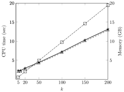
(a) Bitcoin Network

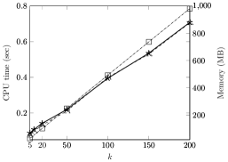
(b) CTU Network

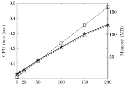
(c) Prosper Loans Network

​​​​ ​​​​

Figure 5. Selective and grouped proportional provenance

7.4. Limiting the scope of provenance tracking

As shown in Section 7.2, proportional provenance tracking throughout the entire history of interactions is infeasible, due to its high memory requirements. In addition, keeping and updating sparse representations of provenance vectors becomes expensive over time as the lists grow larger because of the higher cost of merging operations.

Figure 6 verifies this assertion, by showing the cumulative time and memory requirements while tracking proportional selection after each interaction for the first 500K interactions in Bitcoin and CTU (after this point, the memory requirements become too high), and for all interactions in Prosper Loans. Observe that the cumulative runtime increases superlinearly with the number of interactions and so do the memory requirements (these two are correlated). The average cost for handling each interaction grows as the number of processed interactions increases, which is attributed to the population of the sparse lists that keep the provenance information for each vertex; merging operations on these lists become expensive as they grow.

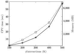
(a) Bitcoin Network

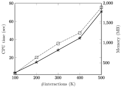
(b) CTU Network

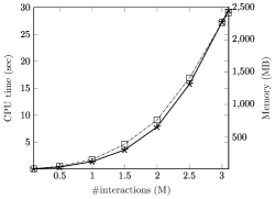
(c) Prosper Loans Network

​​​​ ​​​​

Figure 6. Cumulative time vs. number of processed interactions

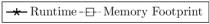
(a) Bitcoin Network

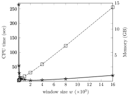
(b) CTU Network

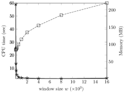
(c) Prosper Loans Network

​​ ​​

Figure 7. Windowing approach

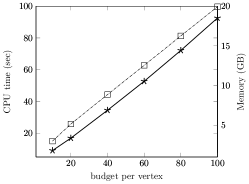
(a) Bitcoin Network

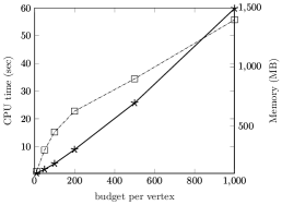
(b) CTU Network

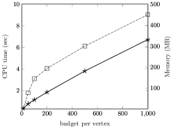
(c) Prosper Loans Network

​​ ​​

Figure 8. Budget-based provenance

We now evaluate the solutions proposed in Section 5.3 for limiting the scope of provenance tracking in order to make the maintenance of proportional provenance vectors feasible for large graphs. Once again, we experimented with the three largest networks and applied the two approaches proposed in Section 5.3 on them. Figure 7 shows the runtime cost and the memory requirements of the windowing approach for different values of the window parameter $W$. As the figure shows, by increasing the size of the window, we improve the runtime performance as the buffers have to be reset less frequently. On the other hand, increasing the window size naturally increases the memory requirements. For Bitcoin and Prosper Loans, larger window sizes are affordable, as the memory requirements do not increase a lot. On the other hand, for CTU the memory requirements almost double when $W$ doubles. In summary, the windowing technique is very useful, especially when we want to have guaranteed accurate provenance information for all vertices up to a time window in the past.

Figure 8 shows the runtime cost and the memory requirements of the budget-based approach for different values of the maximum budget $C$ given as capacity for provenance entries to each vertex. As the figure shows, by increasing the budget $C$ per vertex, the runtime cost to maintain provenance increases, as the provenance information at buffers becomes larger and merging lists becomes more expensive. The increase in the runtime cost is not very high though, because many lists remain relatively short and the number of list shrinks are less frequent. At the same time, the space requirements grow linearly with $C$, which means that very large values of $C$ are not affordable for large graphs like Bitcoin.

In order to assess the value of this approach, in Table 9, we measured for each of the three large datasets and for different values of $C$, (i) the number of times each non-empty buffer has been shrunk and (ii) the percentage of vertices (with non-empty buffer) whose buffer was shrunk at least once. Especially for the larger networks with high memory requirements (Bitcoin and CTU), we observe that the number of shrinks and the percentage of vertices where they take place converge to low values and, after some point, increasing $C$ does not offer much benefit. Overall, the budget-based approach is attractive since each buffer is shrunk only a few times on average, meaning that the provenance information loss is limited even in large graphs. For example, at the Bitcoin network, for a value of $C=50$, each buffer is shrunk 1.5 times on average after 45M interactions, meaning that each buffer tracks provenance information that traces back to tens of millions of transactions before.

Table 9. Shrinking statistics in budget-based provenance

$C$	Bitcoin Network		CTU Network		Prosper Loans Network
	avg. shrinks	% vertices	avg. shrinks	% vertices	avg. shrinks	% vertices
10	1.94	18.38	7.27	31.07	20.67	94.7
50	1.51	14.79	5.1	28.68	4.77	79.29
100	1.43	14.21	4.77	27.94	2.97	69.09
200	–	–	4.53	26.6	2.1	59.16
500	–	–	4.34	25.24	1.5	47.64
1000	–	–	4.3	25.02	1.23	41.39

7.5. Path tracking

As discussed in Section 6, in might be desirable, for each quantity that has reached the buffer of a vertex to know not just the vertex that generated the quantity, but also the path that the quantity followed in the graph until it reached its destination. In the next experiment, we evaluate the overhead of tracking the paths (i.e., how-provenance) compared to just tracking the origins of the quantities. We implemented path tracking as part of the LIFO selection policy for provenance (Section 4.2) and used it to track the paths for all (origin, quantity) pairs accumulated at vertices after processing all interactions in all datasets. Table 10 shows the runtime performance, the memory requirements, and the average path length for each quantity element. The memory requirements are split into the memory required to store the provenance entries in the lists (as in LIFO) and the memory required to store the paths. Observe that for most datasets the memory overhead for keeping the paths is not extremely high. This overhead is determined by the average path length (last column of the table), which is relatively low in four out of the five datasets. Only in Flights the storage overhead for the paths is very high because quantities travel a long way. In this dataset, the number of vertices is very small compared to the number of interactions, so we can expect very long paths. Still, on all datasets, the runtime is only up to a few times higher compared to tracking just the origins and not the paths (see Table 7, column LIFO), meaning that path tracking is feasible even for very long sequences of interactions on large graphs, like Bitcoin.

Table 10. Tracking provenance paths in LIFO

Dataset	time (sec.)	mem entries (MB)	mem paths (MB)	total mem (MB)	avg. path length
Bitcoin	13.35	534.62	847.50	1382.13	4.75
CTU	0.36	33.87	7.16	41.03	0.63
Prosper	0.4	36.85	0.74	37.59	0.06
Flights	0.17	0.627	57.09	57.72	273.17
Taxis	0.008	0.58	1.09	1.68	5.55

7.6. Use case

Figure 9 demonstrates a practical example of provenance tracing in TINs. The plot shows the total accumulated quantities at the vertices of Bitcoin after each interaction (first 100K interactions, proportional selection policy). Consider a data analyst who wants to be alerted whenever a vertex $v$ accumulates a significant amount of money, which does not originate from $v$’s direct neighbors (i.e., $v$’s neighbors just relay amounts to $v$). Hence, after each interaction, we issue an alert when the receiving vertex does not have any quantity that originates from its neighbors and the total quantity in its buffer exceeds 10K BTC. The colored dots in the figure show these alerts (89 in total) and provenance information for some of them. Red dots are alerts where the number of contributing vertices is less than five (the rest of them are blue). We observe that in most cases the amount was received from numerous vertices (an indication of possible “smurfing”). This alerting mechanism is very efficient and easy to implement, as we only have to maintain at each vertex $v$ the total quantity that originates from vertices that transfer quantities to $v$ (i.e., direct neighbors of $v$).

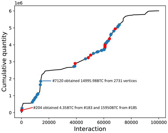
Figure 9. Provenance alerts in Bitcoin

8. Conclusions

In this paper, we introduced and studied provenance in temporal interaction networks (TINs). To the best of our knowledge, we are the first to define and study this problem, considering the data transfers among the vertices, as interactions take place over time. We investigate different selection policies for data propagation in TINs that correspond to different application scenaria. For each policy, we propose propagation mechanisms for provenance (annotation) data and analyze their space and time complexities. For the hardest policy (proportional selection), we propose to track provenance from a limited set of vertices or from groups thereof. We also propose to limit provenance tracking up to a sliding window of past interactions or to set a space budget at each vertex for provenance tracking. We evaluated our methods using five real datasets and demonstrated their scalability. In the future, we plan to investigate lazy approaches for data provenance in TINs (e.g., apply the replay lazy (Glavic et al., 2013) approach, or investigate backtracing methods). In addition, we plan to study whether our approaches for TINs can be adapted to be applied on social networks, where data are diffused, instead on being relayed from vertex to vertex. Finally, we plan to analyze in depth the computed provenance data in TINs, with the help of data mining approaches, in order find interesting insights in them.

References

- (1)
- Agrawal et al. (2006) Parag Agrawal, Omar Benjelloun, Anish Das Sarma, Chris Hayworth, Shubha U. Nabar, Tomoe Sugihara, and Jennifer Widom. 2006. Trio: A System for Data, Uncertainty, and Lineage. In Proceedings of the 32nd International Conference on Very Large Data Bases, Seoul, Korea, September 12-15, 2006. 1151–1154.
- Akrida et al. (2017) Eleni C. Akrida, Jurek Czyzowicz, Leszek Gasieniec, Lukasz Kuszner, and Paul G. Spirakis. 2017. Temporal Flows in Temporal Networks. In Algorithms and Complexity - 10th International Conference, CIAC 2017, Athens, Greece, May 24-26, 2017, Proceedings. 43–54.
- Barbier et al. (2013) Geoffrey Barbier, Zhuo Feng, Pritam Gundecha, and Huan Liu. 2013. Provenance data in social media. Synthesis Lectures on Data Mining and Knowledge Discovery (2013), 1–84.
- Belth et al. ([n.d.]) Caleb Belth, Xinyi Zheng, and Danai Koutra. [n.d.]. Mining Persistent Activity in Continually Evolving Networks. In KDD ’20: The 26th ACM SIGKDD Conference on Knowledge Discovery and Data Mining, Virtual Event, CA, USA, August 23-27, 2020, Rajesh Gupta, Yan Liu, Jiliang Tang, and B. Aditya Prakash (Eds.). 934–944.
- Bhagwat et al. (2004) Deepavali Bhagwat, Laura Chiticariu, Wang Chiew Tan, and Gaurav Vijayvargiya. 2004. An Annotation Management System for Relational Databases. In (e)Proceedings of the Thirtieth International Conference on Very Large Data Bases, VLDB 2004, Toronto, Canada, August 31 - September 3 2004. 900–911.
- Buneman et al. (2001) Peter Buneman, Sanjeev Khanna, and Wang Chiew Tan. 2001. Why and Where: A Characterization of Data Provenance. In Database Theory - ICDT 2001, 8th International Conference. 316–330.
- Buneman et al. (2002) Peter Buneman, Sanjeev Khanna, and Wang Chiew Tan. 2002. On Propagation of Deletions and Annotations Through Views. In PODS. 150–158.
- Chapman et al. (2008) Adriane Chapman, H. V. Jagadish, and Prakash Ramanan. 2008. Efficient provenance storage. In Proceedings of the ACM SIGMOD International Conference on Management of Data, SIGMOD 2008, Vancouver, BC, Canada, June 10-12, 2008. 993–1006.
- Cheney et al. (2009) James Cheney, Laura Chiticariu, and Wang Chiew Tan. 2009. Provenance in Databases: Why, How, and Where. Found. Trends Databases (2009), 379–474.
- Chothia et al. (2016) Zaheer Chothia, John Liagouris, Frank McSherry, and Timothy Roscoe. 2016. Explaining Outputs in Modern Data Analytics. Proc. VLDB Endow. (2016), 1137–1148.
- de Paula et al. (2013) Renato de Paula, Maristela Holanda, Luciana S. A. Gomes, Sérgio Lifschitz, and Maria Emília M. T. Walter. 2013. Provenance in bioinformatics workflows. BMC Bioinform. (2013), S6.
- Decker and Wattenhofer (2013) Christian Decker and Roger Wattenhofer. 2013. Information propagation in the Bitcoin network. In 13th IEEE International Conference on Peer-to-Peer Computing. 1–10.
- Domingos and Richardson (2001) Pedro M. Domingos and Matthew Richardson. 2001. Mining the network value of customers. In Proceedings of the seventh ACM SIGKDD international conference on Knowledge discovery and data mining. 57–66.
- García et al. (2014) Sebastián García, Martin Grill, Jan Stiborek, and Alejandro Zunino. 2014. An empirical comparison of botnet detection methods. Comput. Secur. (2014), 100–123.
- Geerts et al. (2006) Floris Geerts, Anastasios Kementsietsidis, and Diego Milano. 2006. MONDRIAN: Annotating and Querying Databases through Colors and Blocks. In Proceedings of the 22nd International Conference on Data Engineering, ICDE 2006, 3-8 April 2006, Atlanta, GA, USA. 82.
- Glavic et al. (2013) Boris Glavic, Kyumars Sheykh Esmaili, Peter Michael Fischer, and Nesime Tatbul. 2013. Ariadne: managing fine-grained provenance on data streams. In DEBS. ACM, 39–50.
- Green et al. (2010) Todd J. Green, Grigoris Karvounarakis, Zachary G. Ives, and Val Tannen. 2010. Provenance in ORCHESTRA. IEEE Data Eng. Bull. (2010), 9–16.
- Gundecha et al. (2013) Pritam Gundecha, Zhuo Feng, and Huan Liu. 2013. Seeking provenance of information using social media. In 22nd ACM International Conference on Information and Knowledge Management, CIKM. 1691–1696.
- Han et al. (2020) Xueyuan Han, Thomas F. J.-M. Pasquier, Adam Bates, James Mickens, and Margo I. Seltzer. 2020. Unicorn: Runtime Provenance-Based Detector for Advanced Persistent Threats. In 27th Annual Network and Distributed System Security Symposium, NDSS 2020, San Diego, California, USA, February 23-26, 2020.
- Heinis and Alonso (2008) Thomas Heinis and Gustavo Alonso. 2008. Efficient lineage tracking for scientific workflows. In Proceedings of the ACM SIGMOD International Conference on Management of Data, SIGMOD 2008, Vancouver, BC, Canada, June 10-12, 2008. 1007–1018.
- Holme and Saramäki (2012) Petter Holme and Jari Saramäki. 2012. Temporal networks. Physics reports (2012), 97–125.
- Interlandi et al. (2015) Matteo Interlandi, Kshitij Shah, Sai Deep Tetali, Muhammad Ali Gulzar, Seunghyun Yoo, Miryung Kim, Todd D. Millstein, and Tyson Condie. 2015. Titian: Data Provenance Support in Spark. Proc. VLDB Endow. (2015), 216–227.
- Karvounarakis et al. (2010) Grigoris Karvounarakis, Zachary G. Ives, and Val Tannen. 2010. Querying data provenance. In Proceedings of the ACM SIGMOD International Conference on Management of Data, SIGMOD 2010, Indianapolis, Indiana, USA, June 6-10, 2010. 951–962.
- Karypis and Kumar (1998) George Karypis and Vipin Kumar. 1998. A Fast and High Quality Multilevel Scheme for Partitioning Irregular Graphs. SIAM J. Sci. Comput. 20, 1 (1998), 359–392.
- Kempe et al. (2003) David Kempe, Jon M. Kleinberg, and Éva Tardos. 2003. Maximizing the spread of influence through a social network. In Proceedings of the Ninth ACM SIGKDD International Conference on Knowledge Discovery and Data Mining. 137–146.
- Kondor et al. (2013) Dániel Kondor, Márton Pósfai, István Csabai, and Gábor Vattay. 2013. Do the rich get richer? An empirical analysis of the BitCoin transaction network. CoRR (2013).
- Kosyfaki et al. (2019) Chrysanthi Kosyfaki, Nikos Mamoulis, Evaggelia Pitoura, and Panayiotis Tsaparas. 2019. Flow Motifs in Interaction Networks. In Advances in Database Technology - 22nd International Conference on Extending Database Technology, EDBT 2019, Lisbon, Portugal, March 26-29, 2019. 241–252.
- Kosyfaki et al. (2021) Chrysanthi Kosyfaki, Nikos Mamoulis, Evaggelia Pitoura, and Panayiotis Tsaparas. 2021. Flow Computation in Temporal Interaction Networks. In 37th IEEE International Conference on Data Engineering, ICDE 2021, Chania, Greece, April 19-22, 2021. 660–671.
- Kumar and Calders (2017) Rohit Kumar and Toon Calders. 2017. Information Propagation in Interaction Networks. In Proceedings of the 20th International Conference on Extending Database Technology, EDBT. 270–281.
- Lee et al. (2018) Seokki Lee, Bertram Ludäscher, and Boris Glavic. 2018. Provenance Summaries for Answers and Non-Answers. Proc. VLDB Endow. (2018), 1954–1957.
- Lee et al. (2019) Seokki Lee, Bertram Ludäscher, and Boris Glavic. 2019. PUG: a framework and practical implementation for why and why-not provenance. VLDB J. (2019), 47–71.
- Lee et al. (2020) Seokki Lee, Bertram Ludäscher, and Boris Glavic. 2020. Approximate Summaries for Why and Why-not Provenance. Proc. VLDB Endow. (2020), 912–924.
- Li et al. (2017) Aming Li, Sean P Cornelius, Y-Y Liu, Long Wang, and A-L Barabási. 2017. The fundamental advantages of temporal networks. (2017), 1042–1046.
- Masuda and Holme (2013) Naoki Masuda and Petter Holme. 2013. Predicting and controlling infectious disease epidemics using temporal networks. F1000Prime Reports 5, 6 (2013).
- Morris (1985) R. T. Morris. 1985. A Weakness in the 4.2BSD Unix TCP/IP Software. Technical Report #117. Bell Labs Computer Science.
- Namaki et al. (2020) Mohammad Hossein Namaki, Avrilia Floratou, Fotis Psallidas, Subru Krishnan, Ashvin Agrawal, Yinghui Wu, Yiwen Zhu, and Markus Weimer. 2020. Vamsa: Automated Provenance Tracking in Data Science Scripts. In KDD ’20: The 26th ACM SIGKDD Conference on Knowledge Discovery and Data Mining, Virtual Event, CA, USA, August 23-27, 2020. 1542–1551.
- Parulian et al. (2021) Nikolaus Nova Parulian, Timothy M. McPhillips, and Bertram Ludäscher. 2021. A Model and System for Querying Provenance from Data Cleaning Workflows. In Provenance and Annotation of Data and Processes - 8th and 9th International Provenance and Annotation Workshop, IPAW 2020 + IPAW 2021, Virtual Event, July 19-22, 2021, Proceedings. 183–197.
- Polychroniou et al. (2015) Orestis Polychroniou, Arun Raghavan, and Kenneth A Ross. 2015. Rethinking SIMD vectorization for in-memory databases. In Proceedings of the 2015 ACM SIGMOD International Conference on Management of Data. 1493–1508.
- Psallidas and Wu (2018a) Fotis Psallidas and Eugene Wu. 2018a. Demonstration of Smoke: A Deep Breath of Data-Intensive Lineage Applications. In Proceedings of the 2018 International Conference on Management of Data, SIGMOD Conference 2018, Houston, TX, USA, June 10-15, 2018. 1781–1784.
- Psallidas and Wu (2018b) Fotis Psallidas and Eugene Wu. 2018b. Smoke: Fine-grained Lineage at Interactive Speed. Proc. VLDB Endow. (2018), 719–732.
- Richardson and Domingos (2002) Matthew Richardson and Pedro M. Domingos. 2002. Mining knowledge-sharing sites for viral marketing. In Proceedings of the Eighth ACM SIGKDD International Conference on Knowledge Discovery and Data Mining. 61–70.
- Ruan et al. (2019) Pingcheng Ruan, Gang Chen, Tien Tuan Anh Dinh, Qian Lin, Beng Chin Ooi, and Meihui Zhang. 2019. Fine-grained, secure and efficient data provenance on blockchain systems. Proceedings of the VLDB Endowment (2019), 975–988.
- Rupprecht et al. (2020) Lukas Rupprecht, James C. Davis, Constantine Arnold, Yaniv Gur, and Deepavali Bhagwat. 2020. Improving Reproducibility of Data Science Pipelines through Transparent Provenance Capture. Proc. VLDB Endow. (2020), 3354–3368.
- Savage et al. ([n.d.]) Stefan Savage, David Wetherall, Anna R. Karlin, and Thomas E. Anderson. [n.d.]. Practical network support for IP traceback. In Proceedings of the ACM SIGCOMM 2000 Conference on Applications, Technologies, Architectures, and Protocols for Computer Communication, August 28 - September 1, 2000, Stockholm, Sweden. 295–306.
- Taxidou et al. (2015) Io Taxidou, Tom De Nies, Ruben Verborgh, Peter M. Fischer, Erik Mannens, and Rik Van de Walle. 2015. Modeling Information Diffusion in Social Media as Provenance with W3C PROV. In Proceedings of the 24th International Conference on World Wide Web Companion, WWW. 819–824.
- Zhou et al. (2020) Dawei Zhou, Lecheng Zheng, Jiawei Han, and Jingrui He. 2020. A Data-Driven Graph Generative Model for Temporal Interaction Networks. In KDD ’20: The 26th ACM SIGKDD Conference on Knowledge Discovery and Data Mining, Virtual Event, CA, USA, August 23-27, 2020. 401–411.
- Züfle et al. (2018) Andreas Züfle, Matthias Renz, Tobias Emrich, and Maximilian Franzke. 2018. Pattern Search in Temporal Social Networks. In Proceedings of the 21st International Conference on Extending Database Technology, EDBT 2018, Vienna, Austria, March 26-29, 2018. 289–300.