Analytical Ground- and Excited-State Gradients for Molecular Electronic Structure Theory from Hybrid Quantum/Classical Methods

Abstract

We develop analytical gradients of ground- and excited-state energies with respect to system parameters including the nuclear coordinates for the hybrid quantum/classical multistate contracted variational quantum eigensolver (MC-VQE) applied to fermionic systems. We show how the resulting response contributions to the gradient can be evaluated with a quantum effort similar to that of obtaining the VQE energy and independent of the total number of derivative parameters (e.g. number of nuclear coordinates) by adopting a Lagrangian formalism for the evaluation of the total derivative. We also demonstrate that large-step-size finite-difference treatment of directional derivatives in concert with the parameter shift rule can significantly mitigate the complexity of dealing with the quantum parameter Hessian when solving the quantum response equations. This enables the computation of analytical derivative properties of systems with hundreds of atoms, while solving an active space of their most strongly correlated orbitals on a quantum computer. We numerically demonstrate the exactness the analytical gradients and discuss the magnitude of the quantum response contributions.

I Introduction

When performing simulations, computational chemists frequently depend on a toolset of computational methods to provide observables beyond approximations to the state energies for a given arrangement of nuclear cores and electronic quantum numbers. First-order derivatives of the energy and other properties of ground- and excited-state electronic wave functions with respect to various system parameters are frequently sought after quantities. Of particularly broad interest is the nuclear gradient, i.e., the first order derivative of the state energy with respect to the nuclear positions. This nuclear gradient represents the classical force acting on point Born-Oppenheimer nuclei, and is indispensable for the determination of critical points on the potential energy surface, the exploration of reaction landscapes, and the computation of static and dynamic properties of molecular systems.

Due to the necessary layering of different numerical techniques, e.g., the combination of a Hartree-Fock-type method to identify molecular orbitals combined with a post-Hartree-Fock-type method to provide an accurate treatment of the electronic wavefunctions, the usage of intermediate computational parameters is necessary. The values of these parameters often need to be determined by means of nested optimization loops which solve particular sets of nonlinear equations. This makes precise computation of derivatives challenging in both existing classical and forthcoming quantum methods, as “response” cross terms stemming from the chain rule derivatives of the intermediate computational parameters will necessarily contribute to the target total derivatives. In the quantum methods, the difficulty is compounded due to the inability to directly access the wave function.

In classical methods, the efficient computation of the full analytical derivative of an observable with respect to arbitrary system parameters, and particularly including response contributions from the chain-rule terms involving the intermediate computational parameters, has been thoroughly established over the past several decades. A particularly efficient and robust approach for deriving and implementing these gradients is present in the “Lagrangian formalism” promoted by Helgaker and co-workers Helgaker:1982:LAG , which itself grew out of several other historical perspectives on the topic, including the Delgarno-Stewart interchange theorem Dalgarno:1958:245 , the Handy-Schaefer Z-vector formalism Handy:1984:Zvec , and the coupled-perturbed approach used by Yamaguchi and many others Schaefer:1986:new . It remains, however, to fully extend these efficient classical techniques for analytical gradients into the domain of hybrid quantum/classical algorithms for quantum chemistry.

A number of notable studies have already made considerable progress in computing derivatives in hybrid quantum/classical methods for quantum chemistry. In quantum phase estimation (QPE) methods, approaches for the derivative have been considered more than a decade ago Kassal:2009:grad . Our manuscript focuses primarily on methods for NISQ-era preskill2018quantum quantum computing, in which many different variational, semi-variational, or non-variational methods for the state energy have been developed mcclean2017hybrid ; parrish2019quantum ; nakanishi2019subspace ; parrish2019qfd ; urbanek2020chemistry ; ollitrault2020quantum ; huggins2020non ; stair2020multireference ; klymko2021real . In these cases, depending on the variational nature of the method with regard to the parameter(s) to be differentiated, considerable additional response terms may arise in the computation of the analytical gradient. the earliest days of the variational quantum eigensolver (VQE) approach, it has been known to many authors that if only the ground state energy is targeted, the nuclear gradient is analytically extractable from the active space density matrix elements that are used already in the optimization of the VQE entangler parameters, i.e., that the gradient is essentially available simultaneously with the energy due to the variational nature of state-specific VQE McClean:2016:023023 . However, when one considers approaches where the VQE entangler parameters are not optimized to minimize the observable to be differentiated, the resulting method will be non-variational, and nonzero chain rule terms will arise to reflect the response of the VQE entangler parameters to the derivative perturbations. This case commonly arises in methods that target ground and excited states simultaneously, e.g., MC-VQE parrish2019quantum or SS-VQE nakanishi2019subspace (in which case the state-averaged energy is optimized by tuning the VQE entangler parameters in an approach denoted SA-VQE), or in cases where an observable other than the energy is differentiated (e.g., in the computation of polarizabilities or non-adiabatic coupling vectors in state-specific VQE). There may also be response terms stemming from parameters other than the VQE entangler parameters, such as orbital parameters.

There seem to be three broad approaches to dealing with the response terms. The first is to simply ignore the response contribution from to the VQE entangler parameters, noting that in the limit of a universal entangler circuit, the response terms will decay to zero, and that there will be competing error sources from shot and decoherence noise that may overwhelm the magnitude of the response terms. The second is to redefine the method to eliminate the response terms. This was done, e.g., in delgado2021variational , where a state-specific CASSCF was performed to simultaneously optimize the state-specific VQE energy with respect to both the VQE entangler parameters and the orbital parameters. This yields a method which is fully variational, and which in particular does not require the solution of the classical coupled-perturbed Hartree-Fock (CPHF) equations to determine the orbital response terms. However, this method will encounter problems if one tries to differentiate observables other than the state-specific energy or if state-specific CASSCF does not provide a reliable treatment of the electronic structure.The third is to consider the response terms as a natural consequence of a non-variational method, and to try to efficiently include their contribution in the computation of the derivative. Varying levels of efficiency are obtained depending on the formalism used. For instance, a pair of studies of analytical gradients in the non-variational SS-VQE method mitarai2020theory ; Azad2021 explicitly compute the response terms, achieving a correct analytical gradient but with quantum computational cost scaling linearly in the total number of derivative directions. Another study focusing on the non-variational QSE-VQE approach o2019calculating includes the response contributions through a sum-over-states formalism that also induces significant overhead. Recently, we have begun the exploration of the Lagrangian approach for analytical derivatives in the context of the phenomonological ab initio exciton model (AIEM) solved with MC-VQE parrish2019hybrid . There we showed how the Lagrangian formalism could sever the dependency of the computational scaling of the gradient from the number of derivative parameters being sought. However, we still encountered significant computational complexity increase from the nature of the SA-VQE Hessian matrix, which is seemingly much harder to deal with in quantum methods relative to classical methods. We make some progress to mitigate this issue in the present manuscript.

As we were finalizing the present manuscript, a preprint by Arimitsu et al appeared arimitsu2021analytic , which derives and implements the gradients of orbital-optimized fermionic SS-VQE and MC-VQE through a Lagrangian formalism. Similar response equations are encountered as in our prior derivative work parrish2019hybrid or as derived below, but the authors consider neither previous approaches introducing the Lagrangian formalism for non-variational gradients in hybrid quantum/classical methods, nor efficient matrix-vector product techniques for mitigating the complexity of working with the SA-VQE parameter Hessian. The latter consideration, together with unavoidable couplings between the quantum VQE parameters and classical orbital parameters manifests as a restriction of the Arimitsu work to small test cases such as 9-atom cis-TFP. A similar Lagrangian-based approach for the non-adiabatic coupling vector has since appeared yalouz2021analytical .

In the present manuscript, we explore the deployment of the Lagrangian approach to provide the analytical gradient for non-variational hybrid quantum/classical methods with fermionic Hamiltonians. We particularly consider the case where there are nonzero response terms arising from both classical intermediate systems parameters such as orbitals determined by Hartree-Fock-type methods, as well as quantum intermediate system parameters such as VQE entangler circuit parameters determined by SA-VQE. For concreteness, we demonstrate numerical results for the case where the orbitals are chosen by the fractional occupation molecular orbital restricted Hartree-Fock (FON-RHF) method gidopoulos1994hartree ; gidopoulos2002ensemble , and then the ground and excited state wavefunctions are simultaneously optimized in an active space picture via the multistate, contracted variant of VQE (MC-VQE) This method is an analog to the popular FOMO-CASCI method barbatti2006ultrafast ; sellner2013ultrafast of classical electronic structure, for which analytical gradients and non-adiabatic coupling vectors have recently been derived hohenstein2015analytic ; hohenstein2016analytic . However, we leave sufficient detail in the theory section to show how the same approach could be adapted to many other combinations of classical and quantum methods, especially including the case where the quantum and classical intermediate system parameters are globally coupled. We also find that our recently developed quantum number preserving (QNP) approach for efficient fermionic VQE entanglers QNP2021 (itself inspired by and derived from a number of other fermionic VQE entangler approaches peruzzo2014variational ; PhysRevX.6.031007 ; Kandala2017 ; Ryabinkin2018 ; lee2018generalized ; evangelista2019exact ; ganzhorn2019gate ; salis2019short ; Bian2019 ; o2019generalized ; gard2020efficient ; xia2020qubit ; yordanov2020efficient ; khamoshi2020correlating ; matsuzawa2020jastrow ) fits particularly nicely into this framework and allow to obtain high quality ground and excited state properties already at low circuit depth, while also obviating the need to consider any constraints to keep the system responses from falling into symmetry-impure sectors of the qubit Hilbert space.

We also make progress with the SA-VQE Hessian complexity problem encountered in the AIEM gradient manuscript, by showing that a combination of iterative matrix-vector-product-based solution of the SA-VQE response equations with a widely spaced finite difference approach for the SA-VQE matrix-vector products works well in numerical practice. We close by numerically demonstrating the exactness of our method against finite difference, showing the performance of the iterative finite-difference Hessian-vector product method, and exploring the magnitude of the response terms in large test cases.

II Theory

II.1 Lagrangian Formalism for Derivative Properties

As with all gradient theory papers, the topic of the present manuscript is how to efficiently compute derivatives of observables of a quantum system with respect to system parameters, while analytically accounting for any non-physical choices made during the approximate computational description of the quantum system. To simplify the discussion, we will confine ourselves to the common case where the observable in question is the adiabatic (ground or excited) state energy $E^{\Theta}$ corresponding to an orthonormal adiabatic state $|\Psi^{\Theta}\rangle$. We will also restrict ourselves to the symmetric and linear ansatz with the property that the adiabatic energy is the expectation value over the Hamiltonian operator $\hat{H}$ .

$$E^{\Theta}\equiv\langle\Psi^{\Theta}|\hat{H}|\Psi^{\Theta}\rangle$$ (1)

We often require total derivatives of this adiabatic state energy with respect to arbitrary displacements of system parameters of the Hamiltonian $\{\xi\}$. An archetypical example of $\{\xi\}$ is the set of Cartesian positions of the positively-charged nuclei of a molecular system, in which case $E^{\Theta,\xi}$ represents the nuclear gradient of the energy, i.e., the opposite of the classical Born-Oppenheimer force on the nuclei. The desired derivative is,

$$E^{\Theta,\xi}\equiv\frac{\mathrm{d}{E^{\Theta}}}{\mathrm{d}{\xi}}=\langle\Psi^{\Theta}|\frac{\partial\hat{H}}{\partial\xi}|\Psi^{\Theta}\rangle+\langle\Psi^{\Theta}|\hat{H}|\frac{\mathrm{d}{\Psi^{\Theta}}}{\mathrm{d}{\xi}}\rangle+\mathrm{H.C.}$$ (2)

Here, the first term is the Hellmann-Feynman contribution, and is the only nonzero contribution if all parameters in $|\Psi^{\Theta}\rangle$ were chosen to make the state energy $E^{\Theta}$ stationary (definitionally true for all state-specific variational wavefunctions). However, if the wave function contains intermediate computational parameters $\{\theta_{g}\}$ that were chosen to satisfy other conditions than the stationarity of the state energy, the “wave function response” terms will arise,

$$\begin{split}E^{\Theta,\xi}\equiv\frac{\mathrm{d}{E^{\Theta}}}{\mathrm{d}{\xi}}=\langle\Psi^{\Theta}|\frac{\partial\hat{H}}{\partial\xi}|\Psi^{\Theta}\rangle\\ +\sum_{g}\langle\Psi^{\Theta}|\hat{H}|\frac{\partial\Psi^{\Theta}(\{\theta_{g}\})}{\partial\theta_{g}}\rangle\frac{\partial\theta_{g}}{\partial\xi}+\mathrm{H.C.}\end{split}$$ (3)

Structurally identical terms arise whenever the quantity of which the derivative is taken is not the one whose optimization yielded the intermediate computational parameters $\{\theta_{g}\}$.

At the moment, it seems that we will have to solve the the parameter response $\frac{\partial\theta_{g}}{\partial\xi}$ separately for each perturbation $\xi$, which will induce unacceptable rise in complexity of the gradient computation relative to the energy computation. Fortunately, the Lagrangian formalism helps us avoid this. We define,

$$\mathcal{L}^{\Theta}\equiv\langle\Psi^{\Theta}|\hat{H}|\Psi^{\Theta}\rangle+\underbrace{\sum_{g^{\prime}}\tilde{\theta}_{g^{\prime}}C_{g^{\prime}}(\{\theta_{g}\})}_{0}$$ (4)

Here $C_{g^{\prime}}(\{\theta_{g}\})=0$ is the $g^{\prime}$-th clause of a set of $n_{g}$ (nonlinear) equations used to define the parameters $\{\theta_{g}\}$. $\{\tilde{\theta}_{g}\}$ are Lagrange multipliers. Making the Lagrangian stationary with respect to the Lagrange multipliers specifies the method,

$$\frac{\partial\mathcal{L}^{\Theta}}{\partial\tilde{\theta}_{g^{\prime}}}=0\Rightarrow C_{g^{\prime}}(\{\theta_{g}\})=0$$ (5)

Making the Lagrangian stationary with respect to the wave function parameters determines the linear response equations,

$$\frac{\partial\mathcal{L}^{\Theta}}{\partial\theta_{g}}=0\Rightarrow\sum_{g^{\prime}}\frac{\partial C_{g^{\prime}}(\{\theta_{g}\})}{\partial\theta_{g}}\tilde{\theta}_{g^{\prime}}=-\frac{\partial\langle\Psi^{\Theta}|\hat{H}|\Psi^{\Theta}\rangle}{\partial\theta_{g}}$$ (6)

Once the Lagrangian (whose value always equals the energy) is stationary with respect to perturbations in non-variational wave function parameters, the desired derivatives can be taken as partial rather than total derivatives,

$$E^{\Theta,\xi} =\frac{\mathrm{d}{E^{\Theta}}}{\mathrm{d}{\xi}}=\frac{\partial\mathcal{L}}{\partial\hat{H}}\frac{\mathrm{d}{\hat{H}}}{\mathrm{d}{\xi}}$$ (7)

$$=\langle\Psi^{\Theta}|\frac{\partial\hat{H}}{\partial\xi}|\Psi^{\Theta}\rangle+\sum_{g^{\prime}}\tilde{\theta}_{g^{\prime}}\frac{\partial C_{g^{\prime}}(\{\theta_{g}\})}{\partial\hat{H}}\frac{\partial\hat{H}}{\partial\xi}$$ (8)

$$=\left(\frac{\partial E^{\Theta}}{\partial\hat{H}}+\sum_{g^{\prime}}\tilde{\theta}_{g^{\prime}}\frac{\partial C_{g^{\prime}}(\{\theta_{g}\})}{\partial\hat{H}}\right)\frac{\partial\hat{H}}{\partial\xi}$$ (9)

The quantities $\frac{\partial E^{\Theta}}{\partial\hat{H}}$ and $\frac{\partial\mathcal{L}^{\Theta}}{\partial\hat{H}}=\frac{\mathrm{d}{E^{\Theta}}}{\mathrm{d}{\hat{H}}}$ are called the “unrelaxed” and “relaxed” density matrices.

Note that the notation $\frac{\partial}{\partial\hat{H}}$ is meant to imply a sum over the partials of the linear matrix element coefficients in $\hat{H}$.

II.1.1 Nested Classical/Quantum Ansatze

It is often the case in hybrid quantum/classical methods (or even classical/classical methods) that several sequential computations are concatenated to form a complete method. For one instance, one may perform some classical computations to determine the spatial orbitals (defined in terms of classical intermediate computational parameters $\{\theta_{g}^{\mathrm{c}}\}$), and subsequently use these orbitals in a VQE-type computation with state-averaged variational entangler circuits (depending on quantum intermediate computational parameters $\{\theta_{g}^{\mathrm{q}}\}$). The resultant adiabatic energies $E^{\Theta}$ will be variational with respect to neither classical nor quantum intermediate computational parameters. However, the Lagrangian formalism will naturally guide us to a set of response equations which are succinct and maximally separated.

$$\begin{split}\mathcal{L}^{\Theta}\equiv E^{\Theta}(\{\theta_{g}^{\mathrm{q}}\},\{\theta_{g}^{\mathrm{c}}\})&+\sum_{g}\tilde{\theta}_{g}^{\mathrm{q}}C_{g}^{\mathrm{q}}(\{\theta_{g^{\prime}}^{\mathrm{c}}\};\{\theta_{g^{\prime}}^{\mathrm{c}}\})\\ &+\sum_{g}\tilde{\theta}_{g}^{\mathrm{c}}C_{g}^{\mathrm{c}}(\{\theta_{g^{\prime}}^{\mathrm{c}}\})\end{split}$$ (10)

The second line indicates that the equations defining the quantum intermediate computational parameters depend on both the quantum and classical intermediate computational parameters, but the equations defining the classical intermediate computational parameters do not depend on the quantum intermediate computational parameters. This leads to a nested and separated set of response equations,

$$\frac{\partial\mathcal{L}^{\Theta}}{\partial\theta_{g}^{\mathrm{q}}} =0\Rightarrow\sum_{g^{\prime}}\tilde{\theta}_{g^{\prime}}^{\mathrm{q}}\frac{\partial C_{g^{\prime}}^{\mathrm{q}}}{\partial\theta_{g}^{\mathrm{q}}}=-\frac{\partial E^{\Theta}}{\partial\theta_{g}^{\mathrm{q}}}$$ (11)

and

$$\frac{\partial\mathcal{L}^{\Theta}}{\partial\theta_{g}^{\mathrm{c}}} =0\Rightarrow\sum_{g^{\prime}}\tilde{\theta}_{g^{\prime}}^{\mathrm{c}}\frac{\partial C_{g^{\prime}}^{\mathrm{c}}}{\partial\theta_{g}^{\mathrm{c}}}=-\frac{\partial E^{\Theta}}{\partial\theta_{g}^{\mathrm{q}}}-\sum_{g^{\prime}}\tilde{\theta}_{g^{\prime}}^{\mathrm{q}}\frac{\partial C_{g^{\prime}}^{\mathrm{q}}}{\partial\theta_{g}^{\mathrm{c}}}.$$ (12)

Critically, this separates the response computations into quantum and classical portions, with iterative classical/quantum computations avoided in the latter.

In practice, the extra right-hand-side contributions in the classical response equations naturally are accounted for if one uses quantum-relaxed density matrices as input to the classical response equations, as we do below.

Note that if the determination of the classical intermediate computational parameters somehow relied on quantum intermediate computational parameters (e.g., if the orbitals were chosen to minimize the quantum state-averaged energy instead of a classical heuristic), the Lagrangian formalism would guide us to a single, united set of response equations resembling CP-SA-CASSCF equations. This would present no conceptual difficulty, but might require considerable additional hybrid quantum/classical computations to evaluate.

II.2 Active Space Picture

We begin from a classically-determined active space of $M$ orthonormal spatial orbitals $\{\phi_{p}(\vec{r}_{1})\}$ (defined to be real in this work). For each of these spatial orbitals, we compose a pair of spin orbitals $\{\psi_{p}(\vec{x}_{1})\equiv\phi_{p}(\vec{r}_{1})\alpha(s_{1})\}$ and $\{\psi_{\bar{p}}(\vec{x}_{1})\equiv\phi_{p}(\vec{r}_{1})\beta(s_{1})\}$, for a total of $2M$ spin orbitals. When referring to spin orbitals, we use a bar to denote $\beta$ (spin down) orbitals and no bar to denote $\alpha$ (spin up) orbitals. We define a set of fermionic composition operators $\{\hat{p}^{\pm}\}$ and $\{\hat{\bar{p}}^{\pm}\}$ for these spin orbitals obeying the usual fermionic anti-commutation relations.

We are given the classically-determined matrix elements of the active space Hamiltonian, including the self energy $E_{\mathrm{ext}}$ of the external (classically-determined) system, the one-body integrals, including the kinetic energy integrals and the potential integrals of the external system

$$(p|\hat{h}|q) \equiv(p|-\nabla_{1}^{2}/2|q)+(p|\hat{v}_{\mathrm{ext}}|q),$$ (13)

$$\equiv\int_{\mathbb{R}^{3}}\mathrm{d}\vec{r}_{1}\ \phi_{p}(\vec{r}_{1})\left[-\frac{\nabla_{1}^{2}}{2}+\hat{v}_{\mathrm{ext}}(\vec{r}_{1})\right]\phi_{q}(\vec{r}_{1})$$ (14)

and the two-body electron repulsion integrals (ERIs),

$$(pq|rs)\equiv\iint_{\mathbb{R}^{6}}\mathrm{d}\vec{r}_{1}\ \mathrm{d}\vec{r}_{2}\ \phi_{p}(\vec{r}_{1})\phi_{q}(\vec{r}_{1})\frac{1}{r_{12}}\phi_{r}(\vec{r}_{2})\phi_{s}(\vec{r}_{2})$$ (15)

In the present work these are all real quantities due to the real nature of the spatial orbitals. Specific definitions of these integrals depend on the type of active space embedding used (e.g., Hartree-Fock external particles) and on the definitions of the spatial orbitals as shown in the integrals over spatial orbitals. See Appendices A.1 and A.2 for specific definitions for the case of FON-RHF spatial orbitals and RHF core orbital embedding, respectively.

For convenience, we define the modified one-electron integrals,

$$(p|\hat{\kappa}|q)\equiv(p|\hat{h}|q)-\frac{1}{2}\sum_{r}(pr|rq)$$ (16)

The Hamiltonian can now be defined as,

$$\hat{H}\equiv E_{\mathrm{ext}}+\sum_{pq}(p|\hat{\kappa}|q)\hat{E}_{pq}^{+}+\frac{1}{2}\sum_{pqrs}(pq|rs)\hat{E}_{pq}^{+}\hat{E}_{rs}^{+}$$ (17)

where the singlet spin-adapted single substitution operator is,

$$\hat{E}_{pq}^{+}\equiv\hat{p}^{\dagger}\hat{q}+\hat{\bar{p}}^{\dagger}\hat{\bar{q}}$$ (18)

We also define the $\alpha$ number, $\beta$ number, and total spin squared quantum number operators as, respectively,

$$\hat{N}_{\alpha} \equiv\sum_{p}\hat{p}^{\dagger}\hat{p}$$ (19)

$$\hat{N}_{\alpha} \equiv\sum_{p}\hat{\bar{p}}^{\dagger}\hat{\bar{p}}$$ (20)

$$\hat{S}^{2} \equiv\hat{S}_{-}\hat{S}_{+}+\hat{S}_{z}+\hat{S}_{z}^{2}$$ (21)

where

$$\hat{S}_{-} \equiv\sum_{p}\bar{p}^{\dagger}p,\quad\hat{S}_{+}\equiv\sum_{p}p^{\dagger}\bar{p}$$ (22)

We are first tasked with solving the time-independent electronic Schrödinger equation within the active space, subject to strict quantum number constraints ($N_{\alpha}$, $N_{\beta}$, $S$),

$$\hat{H}|\Psi^{\Theta}\rangle =E^{\Theta}|\Psi^{\Theta}\rangle:$$ (23)

$$\langle\Psi^{\Theta}|\Psi^{\Theta^{\prime}}\rangle =\delta_{\Theta\Theta^{\prime}}$$ (24)

$$\hat{N}_{\alpha}|\Psi^{\Theta}\rangle =N_{\alpha}|\Psi^{\Theta}\rangle$$ (25)

$$\hat{N}_{\beta}|\Psi^{\Theta}\rangle =N_{\beta}|\Psi^{\Theta}\rangle$$ (26)

$$\hat{S}^{2}|\Psi^{\Theta}\rangle =S/2(S/2+1)|\Psi^{\Theta}\rangle$$ (27)

We will construct the wavefunctions $\{|\Psi^{\Theta}\rangle\}$ and measure observable properties thereof with the aid of a qubit-based quantum computer. There are many approaches for this hybrid quantum/classical solution of the Schrödinger equation. For concreteness, herein we use the multistate, contracted variant of the variational quantum eigensolver (MC-VQE) for its seamless simultaneous treatment of ground and excited states.

II.3 Target Gradient

We are then asked to evaluate the derivative of the state energy $E^{\Theta}$ with respect to an arbitrary system parameter $\xi$ (e.g., the position of one of the nuclei, an external electric field, etc),

$$E^{\Theta,\xi}\equiv\frac{\mathrm{d}{E^{\Theta}}}{\mathrm{d}{\xi}}$$ (28)

A key intermediate in the mixed quantum/classical methodology used here is the spin-summed active space relaxed density matrix, which has one-particle (OPDM) contribution,

$$\bar{\gamma}_{pq}^{\Theta}\equiv\frac{\mathrm{d}{E^{\Theta}}}{\mathrm{d}{(p|\hat{h}|q)}}$$ (29)

and two-particle (TPDM) contribution,

$$\bar{\Gamma}_{pqrs}^{\Theta}\equiv 2\frac{\mathrm{d}{E^{\Theta}}}{\mathrm{d}{(pq|rs)}}$$ (30)

These quantities should be understood to be relaxed up through all quantum intermediate computational parameters (i.e., to be the döppelgangers of full configuration interaction density matrices in the active space), but do not include or have any context for classical intermediate computational parameters such as orbital definitions.

The reason that these contributions are so important is that the linear, symmetrical expectation value property of our ansatz allows us to write (up through the quantum intermediate computational parameters),

$$\mathcal{L}^{\Theta}=E_{\mathrm{ext}}+\sum_{pq}\bar{\gamma}_{pq}^{\Theta}(p|\hat{h}|q)+\frac{1}{2}\sum_{pqrs}\bar{\Gamma}_{pqrs}^{\Theta}(pq|rs)$$ (31)

And therefore, after considering the properties of the Lagrangian, the desired derivative can be found as,

$$E^{\Theta,\xi}=\frac{\mathrm{d}{}}{\mathrm{d}{\xi}}E_{\mathrm{ext}}+\sum_{pq}\bar{\gamma}_{pq}^{\Theta}\frac{\mathrm{d}{}}{\mathrm{d}{\xi}}(p|\hat{h}|q)+\frac{1}{2}\sum_{pqrs}\bar{\Gamma}_{pqrs}^{\Theta}\frac{\mathrm{d}{}}{\mathrm{d}{\xi}}(pq|rs)$$ (32)

Here the total derivative symbol is used when differentiating the active space molecular integrals to emphasize that these contain both intrinsic and orbital response terms (both classical). In practice, this last line represents a call to a classical CASCI gradient computation, with relaxed active space OPDM/TPDM provided as input.

Note also that we will encounter another set of intermediates in the form of the unrelaxed OPDM,

$$\gamma_{pq}^{\Theta}\equiv\frac{\partial E^{\Theta}}{\partial(p|\hat{h}|q)}=\langle\Psi^{\Theta}|\hat{E}_{pq}^{+}|\Psi^{\Theta}\rangle$$ (33)

and TPDM,

$$\Gamma_{pqrs}^{\Theta}\equiv 2\frac{\partial E^{\Theta}}{\partial(pq|rs)}=\langle\Psi^{\Theta}|\hat{E}_{pq}^{+}\hat{E}_{rs}^{+}|\Psi^{\Theta}\rangle$$ (34)

$$-\mathcal{S}\delta_{qr}\langle\Psi^{\Theta}|\hat{E}_{ps}^{+}|\Psi^{\Theta}\rangle$$

Here the symmetrization operator (a convention) acts as,

$$\mathcal{S}T_{pqrs}=\frac{1}{4}\left[T_{pqrs}+T_{pqsr}+T_{qprs}+T_{qpsr}\right]$$ (35)

These do not include any relaxation terms within the active space, e.g., SA-VQE response terms.

II.4 Fermion-to-Qubit Operator Mapping

Within any hybrid quantum/classical approach for the electronic Schrödinger equation, we require a mapping between the spin orbitals and fermionic composition operators of the electronic structure problem to the qubits and distinguishable two-level composition operators of the quantum computer. There are myriad approaches for this mapping, including (variants of) the Jordan-Wigner, parity, and Bravyi-Kitaev maps. For concreteness, we use the Jordan-Wigner mapping in the present work, as previously outlined by many authors and as previously used within our local quantum-number-preserving (QNP) ansatz for MC-VQE in QNP2021 . This leads directly to the rather verbose representation of the Hamiltonian and quantum number operators as specific linear combinations of Pauli operators in the qubit basis, as detailed in Appendix B. Many techniques have been developed to reduce the verbosity of the representation, notably including the double factorization approach poulin2014trotter ; peng2017highly ; motta2018low ; motta2019efficient ; kivlichan2018quantum ; berry2019qubitization ; matsuzawa2020jastrow ; huggins2021efficient ; cohn2021quantum , composing the Hamiltonian as a sum of groups of simultaneously observable Pauli operators, with each leaf in the sum corresponding to a specific spin-adapted spatial orbital rotation obtained by tensor factorization of the ERIs. For our purposes herein, it is conceptually sufficient to be able to compute the density matrix in the natural representation of the qubit-basis operators, e.g., to be able to compute the expectation value of each Pauli word for a representation of the operators in terms of a linear combination of Pauli operators. In numerical practice, it would surely be advantageous to use a more advanced representation such as double factorization to reduce the measurement cost for each observable. This could be seamlessly adopted to the framework presented here, with the caveat that additional classical response terms might arise if an approximate tensor factorization scheme is used to represent the Hamiltonian operator. We defer such considerations to a later study.

II.5 MC-VQE Active Space Wavefunctions

We formally parametrize the MC-VQE active space wavefunctions as,

$$|\Psi^{\Theta}\rangle\coloneqq\sum_{\Theta^{\prime}}\hat{U}(\{\theta_{g}\})|\Phi^{\Theta^{\prime}}\rangle V_{\Theta^{\prime}\Theta}\coloneqq\sum_{\Theta^{\prime}}|\Gamma^{\Theta^{\prime}}\rangle V_{\Theta^{\prime}\Theta}$$ (36)

Here $\{|\Phi^{\Theta}\rangle\}$ are reference states which are classically and quantumly efficiently describable and preparable. The specific construction of $\{|\Phi^{\Theta}\rangle\}$ is a user choice, subject to the following requirements: (1) the reference states must have definite and proper $N_{\alpha}$, $N_{\beta}$, and $S$ quantum numbers and (2) the procedure used to define the reference states must either contain no auxiliary parameters or must be describable in terms of the solutions of a set of nonlinear equations. For concreteness, herein we choose these reference states to be configuration state functions (CSFs), and they therefore have no additional internal computational parameters. If reference states with auxiliary internal parameters are used, additional quantum response equations may arise below, as occurred when we used configuration interaction singles (CIS) reference states instead of CSFs in our AIEM work.

$\hat{U}(\{\theta_{g}\})$ is a VQE entangler circuit with quantum circuit parameters $\{\theta_{g}\}$. The specific construction of $\hat{U}(\{\theta_{g}\})$ is a user choice, subject to the following two requirements: (1) The circuit operator $\hat{U}(\{\theta_{g}\})$ must commute with the $\hat{N}_{\alpha}$, $\hat{N}_{\beta}$, and $\hat{S}^{2}$ quantum number operators for all parameter choices $\{\theta_{g}\}$ and (2) The parameters of the circuit must be simultaneously optimized as described below. For concreteness, herein we use the quantum number preserving gate fabric circuits defined in our prior work QNP2021 , though many other choices that satisfy (1) and (2) could be used within the formalism derived below.

Once the construction of the VQE entangler circuit is established, the circuits parameters $\{\theta_{g}\}$ are optimized to minimize the state-averaged VQE energy,

$$\theta_{g}^{*}\coloneqq\underset{\theta_{g}}{\mathrm{argmin}}\underbrace{\left(\sum_{\Theta}w_{\Theta}\langle\Gamma^{\Theta}|\hat{H}|\Gamma^{\Theta}\rangle\right)}_{\bar{E}(\{\theta_{g}\})}$$ (37)

Here $\{w_{\Theta}\}$ are user-defined non-increasing state averaging weights. In the above two equations, we define the “entangled reference states” $|\Gamma^{\Theta}\rangle\coloneqq\hat{U}(\{\theta_{g}\})|\Phi^{\Theta}\rangle$. $\hat{H}$ is the molecular Hamiltonian of the system, and can be written in terms of second quantized operators or Pauli operators as linear combinations of the one and two body integrals $(p|\hat{h}|q)$ and $(pq|rs)$.

The weak form of the SA-VQE energy minimization condition is the first-order stationary condition,

$$\frac{\partial}{\partial\theta_{g}}\bar{E}=\frac{\partial}{\partial\theta_{g}}\sum_{\Theta}w_{\Theta}\langle\Gamma^{\Theta}|\hat{H}|\Gamma^{\Theta}\rangle=0$$ (38)

In practice, this condition is used to define the SA-VQE entangler circuit parameters $\{\theta_{g}\}$.

The MC-VQE subspace eigenvectors $V_{\Theta^{\prime}\Theta}$ are chosen to diagonalize the MC-VQE subspace Hamiltonian $\mathcal{H}_{\Theta\Theta^{\prime}}\coloneqq\langle\Gamma^{\Theta}|\hat{H}|\Gamma^{\Theta^{\prime}}\rangle$,

$$\sum_{\Theta^{\prime}}\mathcal{H}_{\Theta\Theta^{\prime}}V_{\Theta^{\prime}\Theta^{\prime\prime}}=V_{\Theta\Theta^{\prime\prime}}E^{\Theta}$$ (39)

additionally subject to the orthonormality constraints,

$$\sum_{\Theta^{\prime\prime}}V_{\Theta\Theta^{\prime\prime}}V_{\Theta^{\prime}\Theta^{\prime\prime}}=\delta_{\Theta\Theta^{\prime}},\sum_{\Theta^{\prime\prime}}V_{\Theta^{\prime\prime}\Theta}V_{\Theta^{\prime\prime}\Theta^{\prime}}=\delta_{\Theta\Theta^{\prime}}$$ (40)

and the MC-VQE state energies $E^{\Theta}$ satisfy,

$$E^{\Theta}=\langle\Psi^{\Theta}|\hat{H}|\Psi^{\Theta}\rangle.$$ (41)

Note that it is sometimes convenient to define the rotated reference state,

$$|\Omega^{\Theta}\rangle\equiv\sum_{\Theta^{\prime}}V_{\Theta^{\prime}\Theta}|\Phi^{\Theta}\rangle:\ |\Psi^{\Theta}\rangle=\hat{U}(\{\theta_{g}\})|\Omega^{\Theta}\rangle$$ (42)

As a linear combination of classical reference states, this is usually an efficient classically and quantumly representable state. The utility of this rotated reference state is that a given MC-VQE eigenstate can be prepared with a single quantum circuit, and therefore observables, derivatives, and unrelaxed properties can be evaluated from observations of a single quantum circuit, e.g.,

$$E^{\Theta}=\langle\Omega^{\Theta}|\hat{U}^{\dagger}(\{\theta_{g}\})\hat{H}\hat{U}(\{\theta_{g}\})|\Omega^{\Theta}\rangle$$ (43)

All in all, MC-VQE can be thought of as a procedure that adjusts the parameters of the entangler circuit such that the subspace spanned by the chosen reference states is rotated into the lowest energy corner of the Hilbert space reachable with the chosen entangler ansatz. The Hamiltonian in this subspace can then be measured and classically diagonalized. This yields variational ground and excited state energies and also recipes to prepare explicitly orthogonal corresponding wave functions, without having to enforce this orthogonality via measurements of overlaps or higher powers of the Hamiltonian. Even if one is not interested in excited state properties MC-VQE can be be an attractive method because its multireference nature also means that its ground state energy may be lower than the energy of any individual state that is preparable via the entangler ansatz from a single reference state.

II.6 MC-VQE Active Space Lagrangian

The “quantum” part of the Lagrangian is,

$$\mathcal{L}^{\Theta}\equiv E^{\Theta}+\sum_{\theta_{g}}\frac{\partial\bar{E}}{\partial\theta_{g}}\lambda_{g}$$ (44)

Here $\{\lambda_{g}\}$ are Lagrange multipliers that enforce the use of the SA-VQE stationary conditions to choose the VQE entangler circuit parameters $\{\theta_{g}\}$,

$$\frac{\partial\mathcal{L}^{\Theta}}{\partial\lambda_{g}}=0\Rightarrow\frac{\partial\bar{E}}{\partial\theta_{g}}=0$$ (45)

Note that one may additionally choose to add terms corresponding to the subspace eigendecomposition (i.e., Lagrangian terms to define $V_{\Theta\Theta^{\prime}}$ as diagonalizing the subspace Hamiltonian and being orthonormal), but the response terms stemming from these contributions are zero due to the variational nature of the eigendecomposition.

II.7 MC-VQE Active Space Gradient

The target of the “quantum” part of the gradient are the spin-summed relaxed OPDM and TPDM [first defined in Eqs. (29) and (30)] in the active spatial orbitals, for which it holds that

$$\bar{\gamma}_{pq}^{\Theta} =\frac{\mathrm{d}{E^{\Theta}}}{\mathrm{d}{(p|\hat{h}|q)}}=\frac{\partial\mathcal{L}^{\Theta}}{\partial(p|\hat{h}|q)}$$ (46)

and

$$\bar{\Gamma}_{pqrs}^{\Theta} =2\frac{\mathrm{d}{E^{\Theta}}}{\mathrm{d}{(pq|rs)}}=2\frac{\partial\mathcal{L}^{\Theta}}{\partial(pq|rs)}.$$ (47)

Due to the properties of the Lagrangian formalism, we do not need to compute the parameter response portions of the following chain rule derivatives explicitly,

$$\bar{\gamma}_{pq}^{\Theta} =\sum_{g}\frac{\partial E^{\Theta}}{\partial\theta_{g}}\frac{\partial\theta_{g}}{\partial(p|\hat{h}|q)}$$ (48)

and

$$\bar{\Gamma}_{pqrs}^{\Theta} =2\sum_{g}\frac{\partial E^{\Theta}}{\partial\theta_{g}}\frac{\partial\theta_{g}}{\partial(pq|rs)}$$ (49)

Instead, the properties of the Lagrangian formalism allow us to compute, e.g.,

$$\bar{\gamma}_{pq}^{\Theta} =\frac{\partial E^{\Theta}}{\partial(p|\hat{h}|q)}+\sum_{g}\frac{\partial^{2}\bar{E}}{\partial(p|\hat{h}|q)\partial\theta_{g}}\lambda_{g}$$ (50)

$$\equiv\gamma_{pq}^{\Theta}+\tilde{\gamma}_{pq}^{\Theta}$$ (51)

directly. The last line shows the popular partition of the density matrix into unrelaxed and response contributions.

II.8 Quantum Observables Required for MC-VQE Energies and Gradients

Inspection of the above reveals that the following classes of quantum observables are needed to compute MC-VQE energies and gradients:

(1) Diagonal Expectation Values:

$$\mathcal{O}^{\Theta}=\langle\Phi^{\Theta}|\hat{U}^{\dagger}(\{\theta_{g}\})\hat{O}\hat{U}^{\dagger}(\{\theta_{g}\})|\Phi^{\Theta}\rangle$$ (52)

Here $\hat{O}$ is usually the Hamiltonian, but could optionally be a quantum number operator or any other symmetric operator. $|\Phi^{\Theta}\rangle$ can be either a reference state or a rotated reference state.

(2) Off-Diagonal Expectation Values:

$$\mathcal{O}^{\Theta\Theta^{\prime}}=\langle\Phi^{\Theta}|\hat{U}^{\dagger}(\{\theta_{g}\})\hat{O}\hat{U}^{\dagger}(\{\theta_{g}\})|\Phi^{\Theta^{\prime}}\rangle$$ (53)

$$=\langle\chi_{+}^{\Theta\Theta^{\prime}}|\hat{U}^{\dagger}(\{\theta_{g}\})\hat{O}\hat{U}^{\dagger}(\{\theta_{g}\})|\chi_{+}^{\Theta\Theta^{\prime}}\rangle/2$$

$$-\langle\chi_{-}^{\Theta\Theta^{\prime}}|\hat{U}^{\dagger}(\{\theta_{g}\})\hat{O}\hat{U}^{\dagger}(\{\theta_{g}\})|\chi_{-}^{\Theta\Theta^{\prime}}\rangle/2$$

Where the classically and quantumly tractable interfering combinations of reference states are,

$$|\chi_{\pm}^{\Theta\Theta^{\prime}}\rangle\equiv\frac{1}{\sqrt{2}}\left[|\Phi^{\Theta}\rangle\pm|\Phi^{\Theta^{\prime}}\rangle\right]$$ (54)

(3) Diagonal Density Matrix Expectation Values:

$$\gamma_{I}\equiv\frac{\partial\mathcal{O}^{\Theta}}{\partial O_{I}}=\langle\Phi^{\Theta}|\hat{U}^{\dagger}(\{\theta_{g}\})\hat{\Pi}_{I}\hat{U}^{\dagger}(\{\theta_{g}\})|\Phi^{\Theta}\rangle$$ (55)

For cases where the operator $\hat{O}$ is composed as a weighted linear combination of “basis operators.”

$$\hat{O}\equiv\sum_{I}O_{I}\hat{\Pi}_{I}$$ (56)

Here the basis operators $\{\hat{\Pi}_{I}\}$ could be, e.g., Pauli words, spin-summed single substitution operators $\hat{E}_{pq}^{+}$, etc. Note in particular that one can classically obtain the density matrix in terms of spin-summed single substitution operators (or products thereof) from the corresponding density matrix in terms of Pauli words if the details of the mapping of the second quantized composition operators to Pauli words is known. We refer to this process as “backtransforming” the density matrix, and refer the reader to Appendix B for more details on the procedure. This procedure can also be adapted to the case where the density matrix is expressed in double factorized representation instead of Pauli word representation.

(4) Diagonal Parameter Gradients:

$$\frac{\partial\mathcal{O}^{\Theta}}{\partial\theta_{g}}=\sum_{P}v_{P}\mathcal{O}^{\Theta}(\{\theta_{g^{\prime}}+\delta_{gg^{\prime}}t_{P}\})$$ (57)

This usually refers to the case where $\{\theta_{g}\}$ are the parameters of the SA-VQE entangler circuit. The equality shows the analytical expression of parameter gradients for quantum circuits in terms of the well-known parameter shift rule or one of its generalizations PhysRevLett.118.150503 ; PhysRevA.98.032309 ; PennyLane ; Mari2021 ; wierichs2021general . Within such rules the derivative of the expectation value with respect to each circuit parameter can be analytically computed as a weighted linear combination of separate observable expectation values evaluated along a widely spaced stencil of displacements of that parameter. The fact that the displacements are widely spaced (e.g., not finite difference) implies that statistical noise does not specifically magnify in this process. The parameter shift displacements and weights $\{<t_{P},v_{P}>\}$ are specific to the eigenstructure of each gate element, and in particular to the corresponding number of unique frequencies in the trigonometric polynomial of the observable tomography along the gate parameter. E.g., simple $\hat{R}_{y}(\theta)$ gates require a 2-point parameter shift rule, a diagonal pair substitution gate $\mathrm{QNP_{PX}}(\theta)$ requires a 4-point parameter shift rule, and a spin-adapted orbital rotation $\mathrm{QNP_{OR}}(\theta)$ requires an 8-point parameter shift rule QNP2021 . Two notes of emphasis are appropriate here for contrast with the later section on approximate parameter shift rules for directional derivatives: (1) for gradients evaluated along single parameter directions, the parameter shift rule is exact with a constant number of stencil points but (2) as soon as a directional derivative that involves a linear combinations of parameter directions is involved, it appears that an exact parameter shift rule requires a linear number of stencil points (essentially computing the full gradient with the original parameter shift rule, and then classically contracting with the desired direction vector).

(5) Diagonal Parameter Hessians:

$$\frac{\partial^{2}\mathcal{O}^{\Theta}}{\partial\theta_{g}\partial\theta_{g^{\prime}}}=\sum_{P}\sum_{Q}v_{P}v_{Q}\mathcal{O}^{\Theta}(\{\theta_{g^{\prime\prime}}+\delta_{gg^{\prime\prime}}t_{P}+\delta_{g^{\prime}g^{\prime\prime}}t_{Q}\})$$ (58)

I.e., a double application of the parameter shift rule. It should be noted that evaluation of the diagonal elements of the Hessian can be obtained in essentially the same linear-scaling effort as the gradient, but the evaluation of the full Hessian requires quadratic-scaling effort Mari2021 ; wierichs2021general . Below we consider an approach to try to reduce the scaling of computations involving the Hessian by considering a Hessian matrix-vector product formalism in concert with widely-spaced finite difference stencils for directional derivatives. The connection between finite difference and parameter-shift gradients have recently been discussed in Mari2021 ; Hubregtsen2021 , albeit in the context of single parameter gradients and not directional derivatives. Note that off-diagonal density matrix elements and/or observable derivatives are also easily obtained by a combination of appropriate rule and the off-diagonal observable expectation value rule.

II.9 SA-VQE Response Equations

In order to obtain the target relaxed density matrices of the quantum gradient, we must first solve the SA-VQE response equations,

$$\frac{\partial\mathcal{L}^{\Theta}}{\partial\theta_{g^{\prime}}}=0\Rightarrow\sum_{g}\frac{\partial^{2}\bar{E}}{\partial\theta_{g^{\prime}}\partial\theta_{g}}\lambda_{g}=-\frac{\partial E^{\Theta}}{\partial\theta_{g}}$$ (59)

As written, the SA-VQE response equations appear to require evaluation and storage of the $\mathcal{O}(N_{\theta}^{2})$ SA-VQE Hessian matrix,

$$\mathcal{A}_{gg^{\prime}}\equiv\frac{\partial^{2}\bar{E}}{\partial\theta_{g^{\prime}}\partial\theta_{g}}$$ (60)

Note that there are a few important limits in which the RHS of the SA-VQE response equations,

$$b_{g}\equiv-\frac{\partial E^{\Theta}}{\partial\theta_{g}}$$ (61)

will be zero and where we can avoid the solution of the SA-VQE response equations: (1) In the case that we only include a single state in the SA-VQE optimization, i.e., using VQE instead of MC-VQE. In this case, the state averaged gradient that is optimized is equivalent to the state-specific RHS gradient, and is therefore zero at the conclusion of the VQE parameter optimization. (2) In the limit that we use a powerful enough entangler circuit to exactly solve the Schrödinger equation for the targeted states. (3) In the limit that we are not at the complete entangler circuit limit, but where the state-specific RHS gradient is accidentally zero for all states sought due to external considerations such as the targeted states being in different spatial symmetry irreps.

II.10 Iterative Solution of the SA-VQE Response Equations

Over the next two sections we will introduce an approach to remove the explicit need for the generation, storage, and manipulation of the SA-VQE Hessian. The aim is to remove the need for a double application of the parameter shift rule, which currently scales as $\mathcal{O}(N_{\theta}^{2})$. This is formally higher scaling than the single application of the parameter shift rule needed for the SA-VQE energy gradient, $\mathcal{O}(N_{\theta})$, i.e., as needed in gradient-based optimization of the SA-VQE entangler circuit parameters. Put another way, the computation of the gradient currently seems to scale higher [$\mathcal{O}(N_{\theta}^{2})$] than the computation of the energy [$\mathcal{O}(N_{\theta})$] due to the cost of evaluating the SA-VQE Hessian before the solution of the response equations. In most classical electronic structure methods, the same scaling can be achieved in both the energy and the gradient. The following procedure is one approach to realizing this scaling reduction for SA-VQE response:

The first step needed in this scaling reduction is to replace the explicit solution of the SA-VQE response equations with an iterative method based on matrix-vector products, e.g., a Krylov-type method. There are many possible and common choices to accomplish this, including but not limited to GMRES, MINRES, BiCGSTAB, SOR, Jacobi, or Gauss-Seidel approaches. Note that we cannot use standard conjugate gradient (CG or PCG) methods here, as the SA-VQE Hessian might be indefinite for numerical reasons. Here we focus on the particularly simple choice of a fixed-point iteration accelerated by Pulay’s Direct Inversion of the Iterative Subspace (DIIS) extrapolation method Pulay:1980:393 ; Pulay:1982:556 , as is often used in the solution of response equations (and also nonlinear parameter optimization equations) in classical electronic structure methods.

The specific procedure is as follows for solving $\hat{A}\vec{\lambda}=\vec{b}$, with a symmetric indefinite linear operator $\hat{A}$ (the SA-VQE Hessian), a RHS of $\vec{b}$ (the negative to the state-specific VQE parameter gradient), a LHS of $\vec{\lambda}$ (the target Lagrangian vector), and an easily obtained and pseudoinverted symmetric preconditioner $\hat{P}$ that approximates $\hat{A}$ in a spectral sense:

1. Initialize the solution vector to the trivial initial guess $\vec{\lambda}=\vec{0}$.

2. Compute the residual $\vec{r}\equiv\vec{b}-\hat{A}\vec{\lambda}$.

3. If the maximum residual is less than a user specified convergence threshold $\delta$, i.e., if $\|\vec{r}\|_{\infty}<\delta$, exit the procedure with the current $\vec{\lambda}$ as the converged Lagrangian solution vector.

4. Compute the preconditions residual $\vec{d}\equiv\hat{P}^{-1}\vec{r}$.

5. Compute the updated solution vector $\vec{\lambda}\leftarrow\vec{\lambda}+\vec{d}$.

6. Add the current values of the state vector $\vec{\lambda}$ and error vector $\vec{r}$ to the DIIS history (note that some implementations may prefer to use $\vec{d}$ as the error vector).

7. Query the DIIS protocol for an extrapolated guess to the solution vector $\vec{\lambda}$.

8. Repeat from Step 2 until convergence is achieved in Step 3 or a maximum number of iterations is reached and the iterative procedure reports failure.

Note the key dependence on the SA-VQE Hessian matrix-vector product operation $\vec{\sigma}(\vec{x})\equiv\hat{A}\vec{x}$ in Step 2. For the preconditioner, herein we use the diagonal of the Hessian (obtainable in $\mathcal{O}(N_{\Theta})$ scaling via the double parameter shift rule PhysRevLett.118.150503 ; PhysRevA.98.032309 ; PennyLane ; Mari2021 ; wierichs2021general as sketched for simpler entangler circuits in our previous derivative work parrish2019hybrid ), conditioned to remove elements with extremely small magnitude. The use of more-advanced preconditioners to improve convergence is an important topic for future research.

The well-known DIIS extrapolation protocol holds a limited history of state and error vector pairs. At each step in the fixed point iteration, the DIIS procedure builds a linear error model, and solves norm-constrained least-squares equations to provide an extrapolated prediction of the converged limit of the fixed-point iteration. The DIIS protocol is easily constructed with a handful of classical linear algebra operations, and can be made to be completely agnostic of the details of the fixed point iteration being considered. DIIS can solve nonlinear systems equations effectively in many cases, and when applied to linear indefinite systems of equations in the manner described above, has been shown to be a form of GMRES. For more information on DIIS, the reader is referred to a number of articles on the classical use of DIIS in classical electronic structure methods Pulay:1980:393 ; Pulay:1982:556 ; csaszar1984geometry ; hamilton1986direct ; hutter1994electronic ; scuseria1986accelerating ; kudin2002black ; chen2011listb ; hu2017projected , as well as our hybrid quantum/classical Jacobi parameter optimization approach which uses DIIS as a convergence accelerator parrish2019jacobi . A complete numerical recipe for the DIIS protocol is laid out in the last of these papers.

II.11 Finite-Difference Approximation of SA-VQE Hessian-Vector Products

Now that we have transformed the SA-VQE response equations into a matrix-vector product formalism, we have a chance at reducing the scaling by considering the specifics of the SA-VQE Hessian-vector product, shown here for an arbitrary trial vector $x_{g}$,

$$\sigma_{g}[x_{g^{\prime}}]\equiv\sum_{g^{\prime}}\mathcal{A}_{gg^{\prime}}x_{g^{\prime}}=\sum_{g^{\prime}}\frac{\partial^{2}\bar{E}}{\partial\theta_{g}\partial\theta_{g^{\prime}}}x_{g^{\prime}}$$ (62)

Considering the specific normalized linear combination of parameters along an auxiliary parameter $\tilde{t}$,

$$\theta_{g^{\prime}}(\tilde{t})\equiv\theta_{g^{\prime}}^{0}+\frac{x_{g^{\prime}}}{\|\vec{x}\|_{2}}\tilde{t}$$ (63)

Then our task is to compute the gradient of the scaled directional derivative of the state-averaged energy in the direction of the trial vector,

$$\sigma_{g}[x_{g^{\prime}}]=\frac{\partial}{\partial\theta_{g}}\frac{\partial\bar{E}}{\partial\tilde{t}}\|\vec{x}\|_{2}$$ (64)

It would be ideal to express the directional derivative $\partial_{\tilde{t}}\bar{E}$ as a widely-spaced parameter-shift-rule-type stencil in $t$,

$$\frac{\partial\bar{E}}{\partial\tilde{t}}\stackrel{{\scriptstyle?}}{{\approx}}\sum_{P}v_{P}\bar{E}(\{\theta_{g^{\prime}}^{0}+\tilde{t}_{P}x_{g}^{\prime}/\|\vec{x}\|_{2}\})$$ (65)

Here $\{<\tilde{t}_{P},\tilde{v}_{P}>\}$ are the points and weights of the parameter-shift-rule-type stencil. If such a stencil is possible with a constant number of points for the directional derivative, the complete SA-VQE Hessian matrix-vector product could be formed in $\mathcal{O}(N_{\theta})$ effort by then applying the usual first-derivative parameter shift rule $\{<t_{Q},v_{Q}>\}$ to each point in the directional derivative stencil to obtain the second derivative in $\theta_{g}$,

$$\sigma_{g}[x_{g^{\prime}}]\approx\sum_{Q}\sum_{P}v_{Q}\tilde{v}_{P}\bar{E}(\{\theta_{g^{\prime}}^{0}+\tilde{t}_{P}x_{g^{\prime}}/\|\vec{x}\|_{2}+\delta_{gg^{\prime}}t_{Q}\})\|\vec{x}\|_{2}$$ (66)

I.e., for each needed SA-VQE Hessian matrix-vector product, we first parameter shift in a constant-scaling stencil along the normal direction of the trial vector $\vec{x}$, and then perform a second parameter shift along each parameter direction to obtain the needed second derivative vector. The second shift can be performed with the usual exact parameter shift rule appropriate for the parameter/gate in question. The first proposed parameter shift rule along the arbitrary trial vector direction does not appear to have an exact solution in less than exponential effort, due to the exponential number of combinations of trigonometric functions in an arbitrary direction in the $N_{\theta}$-dimensional trigonometric landscape of $E(\{\theta_{g}\})$. However, we argue that it is plausible that a widely spaced-finite-difference stencil in $\tilde{t}$ may provide for a highly accurate approximate computation of the directional derivative due to the directionally bandlimited nature of the $N_{\theta}$-dimensional trigonometric landscape of $E(\{\theta_{g}\})$. In particular, if we consider the case of gates all with maximum angular frequency oscillation (i.e., trigonometric polynomial basis function) in parameter space in parameter space of $M(\theta)=\exp(-i\omega\theta)$, where $\omega$ is the maximum angular frequency, then the cut through the parameter space along $\tilde{t}$ is composed of a linear combination of an exponential number of trigonometric polynomial basis functions, but with a maximum angular frequency oscillation of $M^{\prime}(t)=\exp(-i\omega\|\vec{x}\|_{1}/\|\vec{x}\|_{2})$. I.e., the maximum angular frequency along $\tilde{t}$ is $\omega\|\vec{x}\|_{1}/\|\vec{x}\|_{2}\leq\omega\sqrt{N_{\theta}}$. The worst case is achieved for the major diagonal trial vector $x_{g}=1\ \forall\ g$. Overall, the $\sqrt{N_{\theta}}$ worst-case scaling of the maximum frequency of $\bar{E}(\tilde{t})$ indicates that the function is significantly bandlimited along any direction. This leads to the ability to apply widely-spaced finite difference stencils without significant loss of accuracy.

In future work, it may be worth considering an adaptive form of finite difference stencil that changes the step size as a function of $\|\vec{x}\|_{1}/\|\vec{x}\|_{2}$. However, we have empirically found that the application of a simple Newton-Cotes symmetric finite difference stencil with a large and isotropic step size for all $\vec{x}$ works surprisingly well for this application in the numerical examples encountered below.

II.12 Procedure for MC-VQE Energies and Gradients

For clarity, we provide this section to explicitly enumerate the full time-ordered procedure for MC-VQE energies and gradients. Many of these operations have been discussed mathematically above, but the time order and preferred approach for each required quantum observable are highlighted in this section.

MC-VQE Energies:

1. Classically obtain a description of the active space spatial orbitals $\{\phi_{p}(\vec{r}_{1})\}$.

2. Classically obtain the active space matrix elements $E_{\mathrm{ext}}$, $\{(p|\hat{h}|q)\}$, and $\{(pq|rs)\}$.

3. Determine the details of the fermion-to-qubit mapping of the composition operators, Hamiltonian operator, and quantum number operators.

4. Construct the quantum number pure reference states $\{|\Phi^{\Theta}\rangle\}$ for the $N_{\Theta}$ targeted states and for the target quantum numbers $N_{\alpha}$, $N_{\beta}$, and $S$ (the quantum numbers may vary from state to state, though this is not explicitly considered in this work). This included classically determining the ansatz any internal parameters of the reference states, and also designing quantum circuits to efficiently prepare these reference states from the qubit fiducial state $|\vec{0}\rangle$.

5. Construct the conceptual design of a quantum number preserving SA-VQE entangler circuit $\hat{U}(\{\theta_{g}\})$, including gate layout and composition and initial parameter guess.

6. Optimize the SA-VQE energy $\bar{E}(\{\theta_{g}\})$ with user-supplied state averaging weights $\{w_{\Theta}\}$ with respect to the entangler circuit parameters $\{\theta_{g}\}$. There are myriad iterative approaches for this parameter optimization which may rely on quantum expectation values of the Hamiltonian over the diagonal entangled reference states $\bar{E}(\{\theta_{g}\})\equiv\sum_{\Theta}w_{\Theta}\langle\Gamma^{\Theta}|\hat{H}|\Gamma^{\Theta}\rangle$, and/or gradients thereof $\partial_{\theta_{g}}\bar{E}$ as computed by the parameter shift rule.

7. Compute the off-diagonal elements of the MC-VQE subspace Hamiltonian $\{\mathcal{H}_{\Theta\Theta^{\prime}}\equiv\langle\Gamma^{\Theta}|\hat{H}|\Gamma^{\Theta^{\prime}}\rangle\}$ by using differences of Hamiltonian expectation values over entangled interfering combinations of reference states.

8. Classically diagonalize $\mathcal{H}_{\Theta\Theta^{\prime}}$ to obtain the eigenvectors $V_{\Theta^{\prime}\Theta}$ and the corresponding eigenvalues $E^{\Theta}$. The diagonal elements of the subspace Hamiltonian will likely already be available from the SA-VQE energy computation in the previous parameter optimization step. Note that the entangled reference states are defined as $\{|\Gamma^{\Theta}(\{\theta_{g}\})\rangle\equiv\hat{U}(\{\theta_{g}\})|\Phi^{\Theta}\rangle\}$.

9. Optionally classically compute the rotated reference states $\{|\Omega^{\Theta}\rangle\equiv\sum_{\Theta^{\prime}}V_{\Theta^{\prime}\Theta}|\Phi^{\Theta^{\prime}}\rangle\}$, including classical composition and description of corresponding quantum circuit.

MC-VQE Gradients:

1. Compute the state-specific VQE entangler parameter gradient $\partial_{\theta_{g}}E^{\Theta}$, e.g., using the parameter shift rule in concert with Hamiltonian expectation values over the entangled rotated reference state for state $\Theta$.

2. Solve the SA-VQE response equations for RHS of $b_{g}\equiv-\partial_{\theta_{g}}E^{\Theta}$ to obtain the Lagrangian $\lambda_{g}$. This can be accomplished by any combination of the explicit, iterative, or iterative + finite difference SA-VQE Hessian-vector product methods described in Sections II.10 or II.11 above.

3. Compute the unrelaxed state-specific OPDM and TPDM $\gamma_{pq}^{\Theta}\equiv\partial_{(p|\hat{h}|q)}E^{\Theta}$ and $\Gamma_{pqrs}^{\Theta}\equiv\partial_{(pq|rs)}E^{\Theta}$, e.g., using Pauli word expectation values over the entangled rotated reference state for state $\Theta$, followed by backtransformation of the Pauli word expectation values to the spin-summed spatial orbital density matrices.

4. Compute the SA-VQE response contributions to the OPDM and TPDM, e.g., $\tilde{\gamma}_{pq}^{\Theta}\equiv\sum_{g}[\partial_{\theta_{g}}\partial_{(p|\hat{h}|q)}\bar{E}]\lambda_{g}$. This can be done efficiently with a combination of the Pauli-word-type procedure for the unrelaxed OPDM/TPDM and a single application of the parameter shift rule.

5. Add the unrelaxed and SA-VQE response contributions to form the “quantum” relaxed OPDM and TPDM, e.g., $\bar{\gamma}_{pq}^{\Theta}\equiv\gamma_{pq}^{\Theta}+\tilde{\gamma}_{pq}^{\Theta}$.

6. Send the relaxed quantum OPDM and TPDM to the classical electronic structure code to determine the classical response (e.g., orbital response), basis set (e.g., Pulay term), and intrinsic contributions to the gradient. Formally this computes $\mathrm{d}_{\xi}E^{\theta}=\mathrm{d}_{\xi}E_{\mathrm{ext}}+\sum_{pq}\bar{\gamma}_{pq}^{\Theta}\mathrm{d}_{\xi}(p|\hat{h}|q)+\frac{1}{2}\sum_{pqrs}\bar{\Gamma}_{pqrs}^{\Theta}\mathrm{d}_{\xi}(pq|rs)$.

Note that double factorization or other Hamiltonian compression approaches could be substituted anywhere Hamiltonian expectation values or Pauli-to-orbital density matrix computations are encountered.

III Computational Details

For the classical orbital determination, Hamiltonian matrix element evaluation, and gradient evaluation steps, we used RHF and FON-RHF methods in atom-centered Gaussian atomic orbital basis sets as implemented in the Lightspeed + TeraChem code stack. The quantum portions of the MC-VQE energy and gradient approaches defined above were implemented in two independent code stacks; An in-house C++/Python quantum circuit simulator code. This code is capable of evaluating Hamiltonian expectation values via either Pauli expectation value expansion or by direct application of the Hamiltonian to an arbitrary qubit statevector with known $N_{\alpha}$ and $N_{\beta}$ via a Knowles-Handy matrix-vector product method. This is similar in spirit to other implementations proposed recently rubin2021fermionic ; stair2021qforte , though we choose to retain the full $2^{N}$ statevector memory during the computation of the quantum circuit simulation to allow for arbitrary gate decompositions (including intermediate non-number-preserving gates) to be simulated. A code stack leveraging PennyLane PennyLane for automatic differentiation and and OpenFermion OpenFermion for Hamiltonian transformations. Both implementations were cross-checked against each other. As the focus of the present work is to enumerate the complete response-including analytical gradient and to probe the size of response terms for realistic systems, we perform the quantum circuit simulations in the limit of infinite statistical sampling and without decoherence noise channels. Consideration of shot and decoherence noise within the complete MC-VQE energy + gradient workflow is an important topic that we leave for future study.

IV Results

IV.1 Moderate-Scale Test Case

To validate our analytical gradient methodology within a challenging and physically relevant system, we consider the case of cyclohexadiene (specifically cyclohexa-1-3-diene) near one of its minimal energy conical intersections (MECI). Cyclohexadiene exhibits an interesting electrocyclic ring opening reaction with strong enantomeric selectivity upon photoexcitation with UV light near 267 nm. This photochemical reaction is likely representative of general electrocyclic ring-opening reactions in generic 1-3-cyclodiene compounds such as terpenine, pro-vitamin-D3, and many others. Understanding of the non-adiabatic dynamics of this reaction, including yields, timescales, stereochemistry and mechanisms involves significant efforts on both the dynamics and electronic structure.

Herein, we take the geometry of the “ring-closing” MECI from SA-2-$\alpha$-CASSCF(6e, 4o)/6-31G* from Ref wolf2019photochemical . We then treat the system with FOMO-CASCI(6e, 4o, $\beta=0.3$)/6-31G* (Gaussian blurring and same active space and $N_{\mathrm{FOMO}}$ as forthcoming CASCI during the FON-RHF procedure). As FON-RHF and SA-$\alpha$-CASSCF use different metrics for determining the orbitals, the FOMO-CASCI $S_{0}$ and $S_{1}$ states are not exactly at a conical intersection - this is useful as it provides a sort of “canonicalization” of the $S_{0}$ and $S_{1}$ states and allows us to robustly consider FCI vs. MC-VQE treatments within the active space without considering degenerate rotations between states.

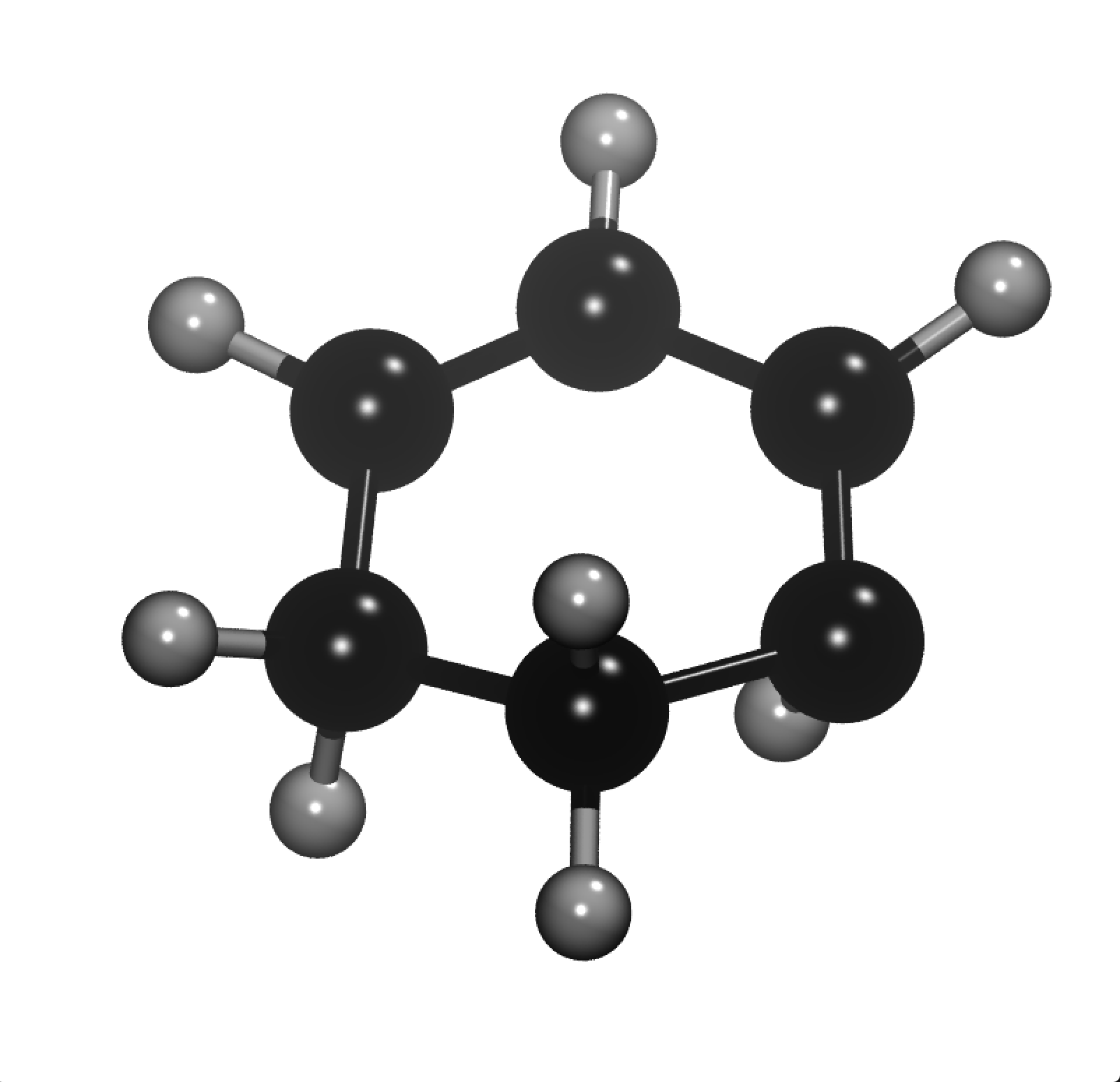
Figure 1: Geometry of “ring-closing” cyclohexadiene MECI computed at SA-2-$\alpha$-CASSCF(6e, 4o)/6-31G* in Ref. wolf2019photochemical and used as a test case within the present manuscript. The lower-right C-H bond is distorted well out of plane, bringing $S_{0}$ and $S_{1}$ states into coincidence without promoting ring-opening photochemistry. A different MECI is responsible for the ring-opening channel of the dynamics.

IV.2 Finite Difference Validation

To validate the correctness of the derived and implemented methodology, we performed finite difference computations with and without SA-VQE response, with finite difference perturbations performed at the level of second-quantized Hamiltonian matrix elements $(p|\hat{h}|q)$ and $(pq|rs)$ and at the level of nuclear gradient computations. These computations indicate that the complete gradient, including SA-VQE response, is concordant with the analytical gradient.

For instance, for the MC-VQE nuclear gradient of the ground state for the cyclohexadiene system considered above, with one “double layer” of QNP entangler gates (one complete layer of even- and odd-pairing QNP gates between spatial orbitals) and two states considered in SA-VQE, the maximum absolute deviation (defined for two nuclear gradients $\vec{G}_{1}$ and $\vec{G}_{2}$ as $M\equiv\|\vec{G}_{1}-\vec{G}_{1}\|_{\infty}$) between the analytical or finite difference CASCI and MC-VQE gradients is $0.016$ a.u., reflecting the incompleteness of the MC-VQE entanglers at this rather coarse level of theory. The maximum absolute deviation between the bare (not including SA-VQE response) MC-VQE gradients and analytical or finite difference MC-VQE gradients is $0.0016$ a.u., indicating that the bare and response-including MC-VQE gradients agree internally to about $10\times$ better than the CASCI and MC-VQE gradients, but that there are still nontrivial response contributions to the gradient. Finally, the SA-VQE-response-including MC-VQE gradients agree with the finite difference MC-VQE gradients to a maximum absolute deviation of $4.6\times 10^{-5}$. This last $~{}\sim 35\times$ reduction in maximum absolute deviation reveals the need for the SA-VQE response contributions to produce the analytical gradient. Further analysis indicates that the conservative maximum magnitude of the response contribution for this case is $\Gamma\equiv\|G_{\mathrm{VQE-Resp}}-G_{\mathrm{VQE-Bare}}\|_{\infty}/\|G_{\mathrm{VQE-Resp}}\|_{\infty}=0.02$, i.e., that the response contribution for this case is $\sim 2\%$ of the maximum analytical gradient entry. This contribution is small but already nontrivial, and will likely become more important in larger cases where VQE entangler is further from completeness, and/or in other derivative contributions that are less stationary than the state energy, e.g., the polarizability or non-adiabatic coupling vector.

IV.3 SA-VQE Hessian Matrix-Vector Product Response Methodology

To probe the potential utility of the iterative solution of the SA-VQE response equations with finite-difference Hessian matrix-vector products and DIIS acceleration, we consider the application of this method to the cyclohexadiene test case with various finite difference stencil sizes $n_{\mathrm{FD}}$ ranging from $2$ to $10$ by even integers and various large finite difference stencil sizes $\Delta_{\mathrm{FD}}\in[0.05,0.1,0.2,0.3]$. As a preliminary, solving the SA-VQE response equations with DIIS without any approximation in the matrix-vector product yields essentially double precision machine epsilon agreement with the explicit pseudoinversion of the full SA-VQE response equation, and requires 5 full iterations of DIIS to reach a convergence in the SA-VQE residual of $\|\vec{r}\|_{\infty}<10^{-9}$.

As Figure 2 shows, the addition of finite difference approximations in the matrix vector products does not appear to significantly affect the accuracy of the resultant gradient, even with small $n_{\mathrm{FD}}$ or large $\Delta_{\mathrm{FD}}$. The maximum absolute errors in the total $S_{0}$ gradient appear to converge roughly geometrically in both the size of the finite difference stencil $n_{\mathrm{FD}}$ and the inverse of the finite difference spacing $\Delta_{\mathrm{FD}}^{-1}$. Remarkably course finite difference grids with, e.g., $(n_{\mathrm{FD}},\Delta_{FD})=(4,0.2)$ already exhibit maximum absolute deviations in the gradient of $<10^{-6}$, i.e., far smaller than the magnitude of the response terms.

One additional potential concern is that the extrinsic introduction of finite difference matrix-vector product formalism might significantly inhibit the convergence of the DIIS iterative procedure. This is addressed in Figures 3 and 4. Here it is found that medium-quality finite difference stencils all show the same convergence behavior, which is qualitative indistinguishable from that of ideal matrix-vector products. Only the coarsest finite difference grids in $\Delta_{\mathrm{FD}}$ and $n_{\mathrm{FD}}$ exhibit noticeable deviations from the ideal convergence behavior. These require only 1 to 2 additional iterations to converge, and the early convergence behavior that this most relevant for the shot-noise limited deployment of VQE is quite similar for all cases.

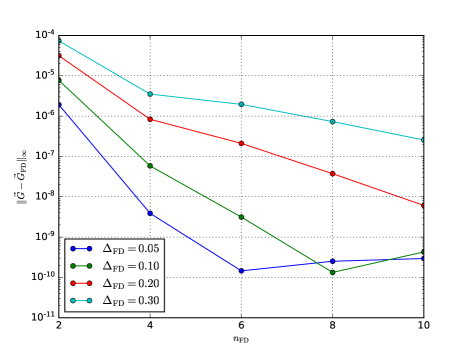
Figure 2: Maximum absolute error in complete nuclear gradient for $S_{0}$ state of cyclohexadiene ring-closing MECI computed with FOMO-CAS-MC-VQE(6e, 4o)/6-31G* with 1 complete layer in the QNP entangler circuit. Here the error is shown as a function of finite difference stencil sizes ($n_{\mathrm{FD}}$) and finite difference step sizes ($\Delta_{\mathrm{FD}}$).

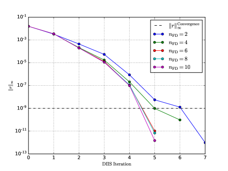
Figure 3: Convergence in the SA-VQE response equations for $S_{0}$ state of cyclohexadiene ring-closing MECI computed with FOMO-CAS-MC-VQE(6e, 4o)/6-31G* with 1 complete layer in the QNP entangler circuit. Here the SA-VQE response residual is shown as a function of DIIS iteration for various finite difference stencil sizes $n_{\mathrm{FD}}$ for finite different step size of $\Delta_{\mathrm{FD}}=0.3$. THe DIIS equations terminate at a convergence criterion of $|\vec{r}|_{\infty}<10^{-9}$.

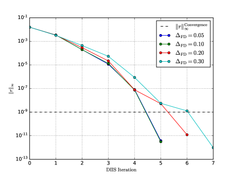
Figure 4: Convergence in the SA-VQE response equations for $S_{0}$ state of cyclohexadiene ring-closing MECI computed with FOMO-CAS-MC-VQE(6e, 4o)/6-31G* with 1 complete layer in the QNP entangler circuit. Here the SA-VQE response residual is shown as a function of DIIS iteration for various finite difference step sizes $\Delta_{\mathrm{FD}}$ for finite difference stencil size of $n_{\mathrm{FD}}=2$. THe DIIS equations terminate at a convergence criterion of $|\vec{r}|_{\infty}<10^{-9}$.

IV.4 Large-Scale Test Case

For a large-scale test case we consider octatetraene solvated by 50 MeOH solvent molecules, with the geometry from snyder2017direct , with 318 atoms. We compute the orbitals with FON-RHF($\beta=0.15$, Gaussian broadening)/6-31G, which comprises 1392 atomic orbitals. This level of theory for classical orbital determination and active space integral preparation/derivative postprocessing is tractable within a few minutes of GPU-accelerated compute time. An active space of (6e, 6o) orbitals is used - note that the intuitively-preferred active space of (8e, 8o) orbitals experiences orbital instabilities between the LUMO+4 and LUMO+5 orbitals with this basis set and geometry.

IV.5 Large-Scale Results

Figure 5 depicts the ground-state gradients of the octatetraene@MeOH${}_{5}0$ test case with a (6e, 6o) active space. Particularly, we compare FCI treatment of the active space wavefunction (red), MC-VQE with two states averaged in SA-VQE and three total layers of QNP entangler gates (blue), and the same MC-VQE without response terms (turquoise). The full Hessian is used in the computation of the response terms, i.e., no finite difference approximations are used. Generally, all three layers of theory agree qualitatively, with some exceptions on the nearest OH group in the prominent lower right MeOH solvent molecule (where an FON-RHF active orbital is hybridizing with those on the octatetraene). The agreement between SA-vQE-response-including and bare MC-VQE gradients are generally within $\sim 2\%$ of the maximum gradient element, and this agreement is much tighter than the agreement between CASCI and MC-VQE for this short depth of SA-VQE entangler. The main conclusion is that external classical system size is not a major issue in computing analytical MC-VQE gradients.

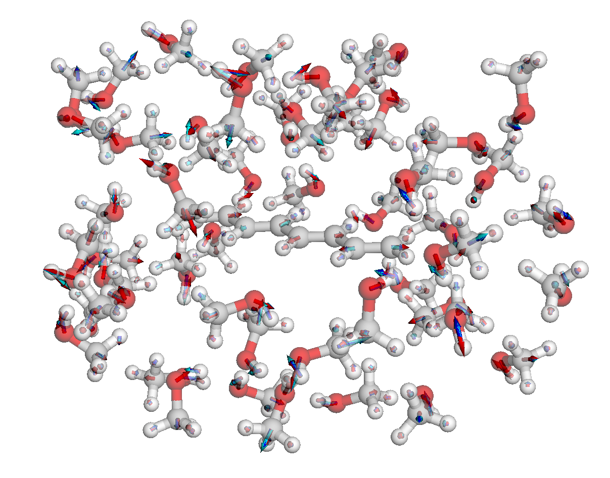
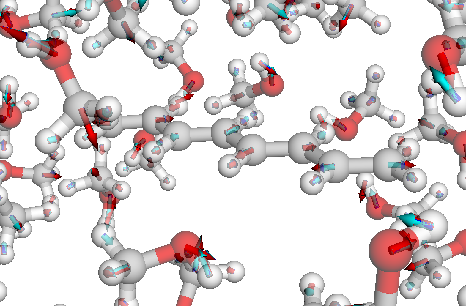
Figure 5: Gradients of singlet ground state of (6e, 6o) active space of octatetraene@MeOH₅₀ with orbitals computed at FON-RHF($\beta=0.15$, Gaussian broadening)/6-31G. Within the active space, gradients are computed with FCI (red), MC-VQE including SA-VQE response (blue) and MC-VQE without SA-VQE response (turquoise). Three total layers of QNP entangler gates are used in SA-VQE response. (Upper panel) Full system. (Lower panel) Inset zoomed in on octatetraene.

V Summary and Outlook

In the present work, we have laid out a complete procedure for the efficient evaluation of analytical first-order derivative properties for nonstationary VQE-type methods with active space embeddings. The use of the Lagrangian formalism is found to remove formal scaling dependencies on the number of derivative perturbations in the computation of the response terms, and also maximally separates the quantum and classical response contributions. Importantly it makes the quantum computational effort independent of the total number of derivative properties, which, e.g., enables the computation of analytical gradients of systems of hundreds of atoms, whose few most important orbitals are accurately simulated on a quantum computer.

The use of a novel iterative SA-VQE Hessian matrix-vector product formalism with widely-spaced finite difference approximations for the needed matrix-vector products is found to remove the need for explicit treatment of the SA-VQE Hessian while retaining an accurate solution of the SA-VQE response equations. Taken together, the Lagrangian approach and iterative matrix-vector product formalism appear to yield a method with similar computational resource requirements for the energy and gradient. Such methodology can be relatively easily adapted to other hybrid quantum/classical approaches, including other non-stationary algorithms such as certain variants of QSE-VQE, SS-VQE, NO-VQE, QFD, or VQPE, and can be extended to other underlying classical methods such as CIS-NO shu2015configuration ; fales2017complete or UNO bofill1989unrestricted orbital determination. Additionally many other target observables and derivative perturbations can be efficiently accessed with this methodology, including polarizabilities, non-adiabatic coupling vectors, and NMR chemical shifts.

There are many interesting directions to pursue from this point. One is an obvious need for a thorough quantification and mitigation of shot-noise and decoherence-noise errors in all steps of the energy and gradient computation. It may well be that much more efficient procedures can be developed if consideration of quantum circuit shot cost is woven throughout the methodology, as has been explored by a number of authors in other context. e.g., Bayesian methods. Another straightforward direction to consider is the use of more-advanced representations of the qubit-basis Hamiltonian operator to reduce measurement burden. Double factorization is surely an interesting direction to pursue along these lines, though additional classical response terms may arise to reflect the approximate nature of the truncated, tensor factorized Hamiltonian in such cases. Higher derivatives could be considered, though it should be noted that in classical electronic structure methodology, higher derivatives are much less prevalent than first derivatives due to the verbosity of implementation and necessary increase in computational scaling when pursuing second and higher-order derivatives.

Another important question is where exactly the SA-VQE response terms need to be explicitly computed. For small systems with deep SA-VQE entangler circuits on very near-term hardware, the shot noise and decoherence noise channels will surely dominate the error, and the simple expedient of using unrelaxed VQE density matrices can be sufficient. I.e., in the simple cases considered herein, the response terms constituted only $\sim 2\%$ of the total gradient. In the longer term, in our opinion (based on numerous experiences with classical methods where response terms can become quite significant in larger systems), it is likely that response terms in VQE methods will eventually become required.

Acknowledgements: QC Ware Corp. acknowledges generous research funding from Covestro Deutschland AG for this project. Covestro acknowledges funding from the German Ministry for Education and Research (BMBF) under the funding program quantum technologies as part of project HFAK (13N15630).

Conflict of Interest: The hybrid quantum/classical Lagrangian technique described in this work is the focus of a US provisional application for patent filed jointly by QC Ware Corp. and Covestro Deutschland AG. RMP and Covestro Deutschland AG own stock/options in QC Ware Corp.

Appendix A Technical Notes: Specific FON-RHF-MC-VQE Ansatz Choices

A.1 Orbital Determination: Fractional Occupation Number Restricted Hartree Fock (FON-RHF)

The fractional occupation number restricted Hartree Fock (FON-RHF) method constructs the real spatial molecular orbitals $\{\phi_{p}(\vec{r}_{1})\equiv\sum_{\mu}C_{\mu p}\chi_{\mu}(\vec{r}_{1})\}$ from the real non-orthogonal atomic orbitals $\{\chi_{\mu}(\vec{r}_{1})\}$, subject to constraints to diagonalize the Fock matrix,

$$f_{pq}\equiv(p|\hat{h}|q)+\sum_{r}2(pq|rr)n_{r}-\sum_{r}(pr|qr)n_{r}=\delta_{pq}\epsilon_{p}$$ (67)

to keep the orbitals orthonormal,

$$(p|q)=\delta_{pq}$$ (68)

and to preserve a target total number of occupied electrons,

$$\sum_{r}n_{r}=N_{\mathrm{FOMO}}$$ (69)

Note that $N_{\mathrm{FOMO}}$ is a user-specified parameter that in practice may be different than the total number of electrons in a subsequent CASCI procedure. However, herein, we use the simple choice of $N_{\mathrm{FOMO}}\equiv N_{\mathrm{T}}$.

The fractional orbital occupation number $n_{r}\in[0,1]$ for each orbital index $r$ is determined by a strictly nonincreasing function in the orbital energy $\epsilon_{r}$. Several popular occupation number functions are used, including the Fermi-Dirac cutoff function,

$$n_{r}^{\mathrm{Fermi-Dirac}}\equiv\frac{1}{1+\exp[\beta(\epsilon_{r}-\mu)]}$$ (70)

and the Gaussian smearing cutoff function,

$$n_{r}^{\mathrm{Gaussian}}\equiv\frac{1}{2}\mathrm{erfc}\left[\beta(\epsilon_{r}-\mu)\right]$$ (71)

In both of these cases, the constant $\beta$ is supplied by the user, and may be roughly interpreted as inverse electronic temperature. The wavefunction parameter $\mu$ is varied to conserve the total electron number constraint, and may be roughly interpreted as the Fermi energy. The FON-RHF occupation numbers may be applied within an active space picture, i.e., the user may elect to clamp the occupation numbers to $1$ for a set of core orbitals, the occupation numbers to $0$ for a set of virtual orbitals, and to let the smooth cutoff procedure provide fractional occupation numbers for a set of active orbitals. Note that the partitions into core/active/virtual subsets may be different from those used in any subsequent CASCI operations, though herein we use the simple choice of coincident core/active/virtual partitions for both the FON-RHF and CASCI/MC-VQE portions of the method.

The FON-RHF orbitals are fully analytically differentiable (except at a topologically small subset of parameter cases involved edge core/active and active/virtual degeneracies in occupation numbers), as shown in several works by other authors. Typically a CASCI analytical gradient procedure built on FON-RHF orbitals involves the following steps: (1) determination of the relaxed density matrix in the active space (e.g., including SA-VQE response) (2) determination of the diagonal relaxed CASCI OPDM and TPDM contributions to the gradient (3) construction and solution of the CP-FON-RHF equations (i.e., classical orbital response) (4) accumulation of the orbital response contributions to the gradient through modified Fock matrix gradients. In particular, once the active-space relaxed MC-VQE TPDM is determined (relaxed to include SA-VQE response), the existing classical FOMO-CASCI gradient code stack handles all of the rest of the computation of the gradient, including all details of the chain-rule gradient contributions of the FON-RHF orbital response, spatial molecular integrals, and nuclear positions. The interested reader is referred for example to Hohenstein’s FOMO-CASCI gradient paper for more details hohenstein2015analytic .

A.2 External System Embedding: Restricted Hartree-Fock

Once the orbitals $\{\phi_{p}(\vec{r}_{1})\}$ have been determined, we partition them into core ($i$, $j$, $k$, $l$), active ($p$, $q$, $r$, $s$) and virtual ($a$, $b$, $c$, $d$) subsets. Using conventional RHF-level embedding of the core orbitals, the active space molecular integrals are,

$$E_{\mathrm{ext}}\equiv E_{\mathrm{Nuc}}+\sum_{i}2(i|\hat{h}|i)+\sum_{ij}2(ii|jj)-\sum_{ij}(ij|ij)$$ (72)

and the one-body Hamiltonian is,

$$(p|\hat{h}|q)\equiv(p|-\nabla_{1}^{2}/2+v_{\mathrm{Nuc}}(\vec{r}_{1})|q)+2\sum_{i}(pq|ii)-\sum_{i}(pi|qi)$$ (73)

Here $E_{\mathrm{Nuc}}$ is the nuclear-nuclear self interaction energy, and $v_{\mathrm{Nuc}}(\vec{r}_{1})$ is the electrostatic potential of the nuclei.

A.3 MC-VQE Reference State Determination: Configuration State Functions

With the spatial orbitals defined and partitioned, we now need to define a pragmatic set of active-space reference states for MC-VQE. Desired characteristics of these states include:

• Classical tractability: These states must be efficiently able to be determined and represented by a polynomial number of classical operations.

• Quantum tractability: These states should be preparable by simple/short quantum circuits, with all needed quantum circuit gate parameters determined a priori by classical computation.

• Orthogonality: For the specific flavor of MC-VQE used here, we require that the reference states be orthonormal. This restriction could be lifted in future work by using a metric-based variant of MC-VQE.

• Physical Relevance: Insofar as possible, these states should approximately span the space of the target Hamiltonian eigenfunctions.

• Quantum number preservation: These states must all be proper eigenfunctions of $\hat{N}_{\alpha}$, $\hat{N}_{\beta}$, and $\hat{S}^{2}$ with the target quantum numbers as eigenvalues.

One pragmatic (but certainly not unique) choice for MC-VQE in fermionic systems is the set of certain configuration state functions (CSFs) in the given qubit orbital basis (i.e., the FON-RHF orbital basis). For instance, for singlet states, we will include the RHF CSF,

$$|\Phi_{0}\rangle\equiv\sum_{i}^{N_{\alpha}}i^{\dagger}\bar{i}^{\dagger}|\rangle$$ (74)

the set of singlet singly-excited CSFs,

$$|\Phi_{i\rightarrow a}^{\mathrm{S}}\rangle\equiv\frac{1}{\sqrt{2}}\left[a^{\dagger}i+\bar{a}^{\dagger}\bar{i}\right]|\Phi_{0}\rangle$$ (75)

and the set of diagonal doubly-excited CSFs,

$$|\Phi_{i\rightarrow a}^{\mathrm{D}}\rangle\equiv a^{\dagger}i\bar{a}^{\dagger}\bar{i}|\Phi_{0}\rangle$$ (76)

For a given target number of MC-VQE states, we limit ourselves to a discrete subset of these via a selection procedure. For instance, we may elect to sort the energies of the reference states and then take lowest few sorted reference states to be the working set for MC-VQE. We may also choose the reference states according to character, i.e., by choosing those that maximize the overlap with states from a nearby geometry during dynamics or geometry optimization.

Appendix B Technical Notes: Jordan Wigner Hamiltonian

For complete details on the logically $\alpha$-then-$\beta$ and physically interleaved flavor of the Jordan-Wigner mapping used herein, and for additional definitions of the Jordan-Wigner forms of the fermionic composition, substitution, $\hat{N}_{\alpha}$, $\hat{N}_{\beta}$, and $\hat{S}^{2}$ operators, the reader is referred to Appendix B of our manuscript on quantum number preserving entangler circuit.

In order to provide a completely closed procedure for the computation of the active space density matrices, we must provide a differentiable mapping between the second-quantized Hamiltonian operator and corresponding qubit compatible operators such as Pauli operators. The primary reason for this is to provide a closed recipe for the backtransformation from qubit-basis observables to the unrelaxed OPDM/TPDM. E.g., if the Hamiltonian is written in Pauli words $\{\hat{\Pi}_{I}\}$ as $\hat{H}\equiv\sum_{I}\mathcal{H}_{I}\hat{\Pi}_{I}$, and we define the Pauli-basis unrelaxed density matrix elements $\{\Gamma_{I}\}$ as,

$$\Gamma_{I}\equiv\langle\Psi^{\Theta}|\hat{\Pi}_{I}|\Psi^{\Theta}\rangle$$ (77)

then we can exploit the equality of the energy trace formulae,

$$E^{\Theta}=E_{\mathrm{ext}}+\sum_{pq}\gamma_{pq}^{\Theta}(p|\hat{h}|q)+\frac{1}{2}\sum_{pqrs}\Gamma_{pqrs}^{\Theta}(pq|rs)$$ (78)

$$=\sum_{I}\mathcal{H}_{I}\Gamma_{I}$$

to obtain the backtransformation formulae,

$$\Rightarrow\gamma_{pq}^{\Theta}=\sum_{I}\frac{\partial\mathcal{H}_{I}}{\partial(p|\hat{h}|q)}\Gamma_{I}^{\Theta}$$ (79)

and,

$$\Rightarrow\Gamma_{pqrs}^{\Theta}=2\sum_{I}\frac{\partial\mathcal{H}_{I}}{\partial(pq|rs)}\Gamma_{I}^{\Theta}$$ (80)

These backtransformation formulae are highly sparse, and are easily performed in classical postprocessing. Below, we show the simplified definition of the Hamiltonian operator in terms of qubit Pauli operators under the Jordan-Wigner mapping.

As discussed in the main text, such a laborious enumeration in Pauli operators is conceptually straightforward, but has been superseded in numerical practice by more-advanced techniques such as double factorization (DF). This does not present any theoretical barrier to computing the active space density matrices, so long as the qubit basis operators of the more advanced representation are fully differentiable with respect to $(p|\hat{h}|q)$ and $(pq|rs)$.

After expansion in labelled spin orbitals, the Hamiltonian is,

$$\hat{H}=\sum_{pq}(p|\hat{h}|q)\left(p^{+}q+\bar{p}^{+}\bar{q}\right)$$ (81)

$$+\frac{1}{2}\sum_{pqrs}(pq|rs)\left[p^{+}r^{+}sq+p^{+}\bar{r}^{+}\bar{s}q+\bar{p}^{+}r^{+}s\bar{q}+\bar{p}^{+}\bar{r}^{+}\bar{s}\bar{q}\right]$$

$$=\sum_{pq}(p|\hat{h}|q)\left(p^{+}q+\bar{p}^{+}\bar{q}\right)$$

$$+\frac{1}{2}\sum_{pqrs}(pq|rs)\left[2\bar{p}^{+}\bar{q}r^{+}s+p^{+}r^{+}sq+\bar{p}^{+}\bar{r}^{+}\bar{s}\bar{q}\right]$$

The following terms enter the Jordan-Wigner Hamiltonian:

One-particle $\alpha$,

$$\hat{H}\leftarrow+\frac{1}{2}\sum_{p}(p|\hat{h}|p)\hat{I}-\frac{1}{2}\sum_{p}(p|\hat{h}|p)\hat{Z}_{p}$$ (82)

$$+\frac{1}{2}\sum_{p<q}(p|\hat{h}|q)\hat{X}_{p}\otimes\hat{Z}_{p+1,q-1}^{\leftrightarrow}\otimes\hat{X}_{q}$$

$$+\frac{1}{2}\sum_{p<q}(p|\hat{h}|q)\hat{Y}_{p}\otimes\hat{Z}_{p+1,q-1}^{\leftrightarrow}\otimes\hat{Y}_{q}$$

One-particle $\beta$,

$$\hat{H}\leftarrow+\frac{1}{2}\sum_{p}(p|\hat{h}|p)\hat{I}-\frac{1}{2}\sum_{p}(p|\hat{h}|p)\hat{Z}_{\bar{p}}$$ (83)

$$+\frac{1}{2}\sum_{p<q}(p|\hat{h}|q)\hat{X}_{\bar{p}}\otimes\hat{Z}_{\bar{p}+1,\bar{q}-1}^{\leftrightarrow}\otimes\hat{X}_{\bar{q}}$$

$$+\frac{1}{2}\sum_{p<q}(p|\hat{h}|q)\hat{Y}_{\bar{p}}\otimes\hat{Z}_{\bar{p}+1,\bar{q}-1}^{\leftrightarrow}\otimes\hat{Y}_{\bar{q}}$$

Two-particle $\alpha$-$\beta$,

$$\hat{H}\leftarrow\frac{1}{4}\sum_{p}\sum_{r}(pp|rr)-\frac{1}{4}\sum_{p}\sum_{r}(pp|rr)\hat{Z}_{\bar{r}}$$ (84)

$$-\frac{1}{4}\sum_{p}\sum_{r}(pp|rr)\hat{Z}_{p}+\frac{1}{4}\sum_{p}\sum_{r}(pp|rr)\hat{Z}_{p}\otimes\hat{Z}_{\bar{r}}$$

$$+\frac{1}{4}\sum_{p}\sum_{r<s}(pp|rs)\hat{X}_{\bar{r}}\leftrightarrow\hat{X}_{\bar{s}}+\frac{1}{4}\sum_{p}\sum_{r<s}(pp|rs)\hat{Y}_{\bar{r}}\leftrightarrow\hat{Y}_{\bar{s}}$$

$$-\frac{1}{4}\sum_{p}\sum_{r<s}(pp|rs)\hat{Z}_{p}\hat{X}_{\bar{r}}\leftrightarrow\hat{X}_{\bar{s}}-\frac{1}{4}\sum_{p}\sum_{r<s}(pp|rs)\hat{Z}_{p}\hat{Y}_{\bar{r}}\leftrightarrow\hat{Y}_{\bar{s}}$$

$$+\frac{1}{4}\sum_{p<q}\sum_{r}(pq|rr)\hat{X}_{p}\leftrightarrow\hat{X}_{q}+\frac{1}{4}\sum_{p<q}\sum_{r}(pq|rr)\hat{Y}_{p}\leftrightarrow\hat{Y}_{q}$$

$$-\frac{1}{4}\sum_{p<q}\sum_{r}(pq|rr)\hat{Z}_{\bar{r}}\hat{X}_{p}\leftrightarrow\hat{X}_{q}-\frac{1}{4}\sum_{p<q}\sum_{r}(pq|rr)\hat{Z}_{\bar{r}}\hat{Y}_{p}\leftrightarrow\hat{Y}_{q}$$

$$+\frac{1}{4}\sum_{p<q}\sum_{r<s}(pq|rs)\hat{X}_{p}\leftrightarrow\hat{X}_{q}\hat{X}_{\bar{r}}\leftrightarrow\hat{X}_{\bar{s}}$$

$$+\frac{1}{4}\sum_{p<q}\sum_{r<s}(pq|rs)\hat{X}_{p}\leftrightarrow\hat{X}_{q}\hat{Y}_{\bar{r}}\leftrightarrow\hat{Y}_{\bar{s}}$$

$$+\frac{1}{4}\sum_{p<q}\sum_{r<s}(pq|rs)\hat{Y}_{p}\leftrightarrow\hat{Y}_{q}\hat{X}_{\bar{r}}\leftrightarrow\hat{X}_{\bar{s}}$$

$$+\frac{1}{4}\sum_{p<q}\sum_{r<s}(pq|rs)\hat{Y}_{p}\leftrightarrow\hat{Y}_{q}\hat{Y}_{\bar{r}}\leftrightarrow\hat{Y}_{\bar{s}}$$

The same-spin terms are, e.g., for $\alpha\alpha$,

$$\hat{H}\leftarrow\frac{1}{4}\sum_{p<q}\langle pq||pq\rangle$$ (85)

$$-\frac{1}{4}\sum_{p}\left[\sum_{q}\langle pq||pq\rangle\right]\hat{Z}_{p}$$

$$+\frac{1}{4}\sum_{p<q}\langle pq||pq\rangle\hat{Z}_{p}\otimes\hat{Z}_{q}$$

$$\frac{1}{4}\sum_{q<r}\left[\sum_{p}\langle pq||pr\rangle\right]\hat{X}_{q}\leftrightarrow\hat{X}_{r}$$

$$+\frac{1}{4}\sum_{q<r}\left[\sum_{p}\langle pq||pr\rangle\right]\hat{Y}_{q}\leftrightarrow\hat{Y}_{r}$$

$$-\frac{1}{4}\sum_{q<r}\sum_{p\neq q,r}\langle pq||pr\rangle\hat{Z}_{p}\hat{X}_{q}\leftrightarrow\hat{X}_{r}$$

$$-\frac{1}{4}\sum_{q<r}\sum_{p\neq q,r}\langle pq||pr\rangle\hat{Z}_{p}\hat{Y}_{q}\leftrightarrow\hat{Y}_{r}$$

$$+\frac{1}{4}\sum_{p<q<r<s}[(pq|rs)-(ps|qr)]X_{p}\leftrightarrow X_{q}X_{r}\leftrightarrow X_{s}$$

$$+\frac{1}{4}\sum_{p<q<r<s}[(pq|rs)-(pr|qs)]X_{p}\leftrightarrow X_{q}Y_{r}\leftrightarrow Y_{s}$$

$$+\frac{1}{4}\sum_{p<q<r<s}[(pr|qs)-(ps|qr)]X_{p}\leftrightarrow Y_{q}Y_{r}\leftrightarrow X_{s}$$

$$+\frac{1}{4}\sum_{p<q<r<s}[(pr|qs)-(ps|qr)]Y_{p}\leftrightarrow X_{q}X_{r}\leftrightarrow Y_{s}$$

$$+\frac{1}{4}\sum_{p<q<r<s}[(pq|rs)-(pr|qs)]Y_{p}\leftrightarrow Y_{q}X_{r}\leftrightarrow X_{s}$$

$$+\frac{1}{4}\sum_{p<q<r<s}[(pq|rs)-(ps|qr)]Y_{p}\leftrightarrow Y_{q}Y_{r}\leftrightarrow Y_{s}$$

And similarly in $\beta\beta$ by “barring” of indices.

Here, the antisymmetrized two-electron integrals are,

$$\langle pq||rs\rangle\equiv\langle pq|rs\rangle-\langle pq|sr\rangle=(pr|qs)-(ps|qr)$$ (86)

Note the 8-fold antisymmetry,

$$\langle pq||rs\rangle=-\langle pq||sr\rangle=-\langle qp||rs\rangle=\langle qp||sr\rangle$$ (87)

$$=\langle rs||pq\rangle=-\langle rs||qp\rangle=-\langle sr||pq\rangle=\langle sr||qp\rangle$$

Also note that the antisymmetry mandates,

$$\langle pp||rs\rangle=\langle pq||rr\rangle=0$$ (88)

B.1 Detailed Derivation of Same-Spin Two-Electron Hamiltonian Term

The same-spin two-electron component of the Hamiltonian can be written (e.g., in $\alpha$) as,

$$\hat{H}^{\alpha\alpha}\equiv\sum_{pqrs}\frac{1}{4}\langle pq||rs\rangle p^{+}q^{+}sr$$ (89)

$$=\sum_{p<q}\sum_{r<s}\langle pq||rs\rangle p^{+}q^{+}sr$$

First up, the cases with full contraction, $(p=r),\ (q=s)$, and $(p=s),\ (q=r)$, but (enforced by the antisymmetrized integrals) $(p\neq q)$ and $(r\neq s)$.

$$H^{\alpha\alpha}\leftarrow\frac{1}{4}\sum_{pq}\langle pq||pq\rangle p^{+}q^{+}qp+\langle pq||qp\rangle p^{+}q^{+}pq$$ (90)

$$=\frac{1}{2}\sum_{pq}\langle pq||pq\rangle p^{+}pq^{+}q$$

$$=\frac{1}{8}\sum_{pq}\langle pq||pq\rangle(\hat{I}_{p}-\hat{Z}_{p})(\hat{I}_{q}-\hat{Z}_{q})$$

$$=\frac{1}{4}\sum_{p<q}\langle pq||pq\rangle-\frac{1}{4}\sum_{p}\left(\sum_{q}\langle pq||pq\rangle\right)\hat{Z}_{p}$$

$$+\frac{1}{4}\sum_{p<q}\langle pq||pq\rangle\hat{Z}_{p}\otimes\hat{Z}_{q}$$

Now, let us consider the case with a single contraction. There are four cases:
$p=r$ $p\neq q$, $r\neq s$ $\Rightarrow p\neq s$
$p=s$ $p\neq q$, $r\neq s$ $\Rightarrow p\neq r$
$q=r$ $p\neq q$, $r\neq s$ $\Rightarrow q\neq s$
$q=s$ $p\neq q$, $r\neq s$ $\Rightarrow q\neq r$

Below $\sum_{pqr}^{\prime}\equiv\sum_{p\neq q\neq r}$,

$$H^{\alpha\alpha}\leftarrow\frac{1}{4}\sum_{pqs}^{\prime}\langle pq||ps\rangle p^{+}q^{+}sp+\frac{1}{4}\sum_{pqr}^{\prime}\langle pq||rp\rangle p^{+}q^{+}pr$$ (91)

$$+\frac{1}{4}\sum_{pqs}^{\prime}\langle pq||qs\rangle p^{+}q^{+}sq+\frac{1}{4}\sum_{pqr}^{\prime}\langle pq||rq\rangle p^{+}q^{+}qr$$

$$=\sum_{pqr}^{\prime}\langle pq||pr\rangle p^{+}pq^{+}r$$

$$=\frac{1}{4}\sum_{p}\sum_{q<r}\langle pq||pr\rangle(\hat{I}_{p}-\hat{Z}_{p})\left[\hat{X}_{q}\leftrightarrow\hat{X}_{r}+\hat{Y}_{q}\leftrightarrow\hat{Y}_{r}\right]$$

$$=\frac{1}{4}\sum_{q<r}\left[\sum_{p}\langle pq||pr\rangle\right]\hat{X}_{q}\leftrightarrow\hat{X}_{r}+\frac{1}{4}\sum_{q<r}\left[\sum_{p}\langle pq||pr\rangle\right]\hat{Y}_{q}\leftrightarrow\hat{Y}_{r}$$

$$-\frac{1}{4}\sum_{q<r}\sum_{p\neq q,r}\langle pq||pr\rangle\hat{Z}_{p}\hat{X}_{q}\leftrightarrow\hat{X}_{r}-\frac{1}{4}\sum_{q<r}\sum_{p\neq q,r}\langle pq||pr\rangle\hat{Z}_{p}\hat{Y}_{q}\leftrightarrow\hat{Y}_{r}$$

Note how the $\hat{Z}_{p}$ puts a hole in the $\leftrightarrow$ string if $q<p<r$.

Finally, let us consider the case with no contraction, $p\neq q\neq r\neq s$,

$$H^{\alpha\alpha}\leftarrow\sum_{p<q<r<s}2\langle pq||rs\rangle p^{+}q^{+}sr$$ (92)

$$+2\langle pr||qs\rangle p^{+}r^{+}sq+2\langle ps||qr\rangle p^{+}s^{+}rq$$

This can be obtained by enumerating all 24 permutations of $pqrs$ and then simplifying to 3 terms by the 8-fold antisymmetry of the integrals/composition operators, or by enumerating all 24 permutations of $pqrs$ and sieving by $p^{\prime}<q^{\prime}$ and $r^{\prime}<q^{\prime}$ restrictions in the bra/ket of the antisymmetrized integrals. Expanding the antisymmetrized integrals,

$$\hat{H}^{\alpha\alpha}\leftarrow 2\sum_{p<q<r<q}\left[(pr|qs)-(ps|qr)\right]p^{+}q^{+}sr$$ (93)

$$+\left[(pq|rs)-(ps|rq)\right]p^{+}r^{+}sq+\left[(pq|sr)-(pr|qs)\right]p^{+}s^{+}rq$$

$$2\sum_{p<q<r<s}(pq|rs)[p^{+}r^{+}sq+p^{+}s^{+}rq]$$

$$+(pr|qs)[p^{+}q^{+}sr-p^{+}s^{+}rq]$$

$$+(ps|qr)[-p^{+}q^{+}sr-p^{+}r^{+}sq]$$

$$=\frac{1}{4}\sum_{p<q<r<q}(pq|rs)[X_{p}\leftrightarrow X_{q}X_{r}\leftrightarrow X_{s}+X_{p}\leftrightarrow X_{q}Y_{r}\leftrightarrow Y_{s}$$

$$+Y_{p}\leftrightarrow Y_{q}X_{r}\leftrightarrow X_{s}+Y_{p}\leftrightarrow Y_{q}Y_{r}\leftrightarrow Y_{s}]$$

$$+(pr|qs)[-X_{p}\leftrightarrow X_{q}Y_{r}\leftrightarrow Y_{s}+X_{p}\leftrightarrow Y_{q}Y_{r}\leftrightarrow X_{s}$$

$$+Y_{p}\leftrightarrow X_{q}X_{r}\leftrightarrow Y_{s}-Y_{p}\leftrightarrow Y_{q}X_{r}\leftrightarrow X_{s}]$$

$$+(ps|qr)[-X_{p}\leftrightarrow X_{q}X_{r}\leftrightarrow X_{s}-X_{p}\leftrightarrow Y_{q}Y_{r}\leftrightarrow X_{s}$$

$$-Y_{p}\leftrightarrow X_{q}X_{r}\leftrightarrow Y_{s}-Y_{p}\leftrightarrow Y_{q}Y_{r}\leftrightarrow Y_{s}]$$

$$=\frac{1}{4}\sum_{p<q<r<s}[(pq|rs)-(ps|qr)]X_{p}\leftrightarrow X_{q}X_{r}\leftrightarrow X_{s}$$

$$+[(pq|rs)-(pr|qs)]X_{p}\leftrightarrow X_{q}Y_{r}\leftrightarrow Y_{s}$$

$$+[(pr|qs)-(ps|qr)]X_{p}\leftrightarrow Y_{q}Y_{r}\leftrightarrow X_{s}$$

$$+[(pr|qs)-(ps|qr)]Y_{p}\leftrightarrow X_{q}X_{r}\leftrightarrow Y_{s}$$

$$+[(pq|rs)-(pr|qs)]Y_{p}\leftrightarrow Y_{q}X_{r}\leftrightarrow X_{s}$$

$$+[(pq|rs)-(ps|qr)]Y_{p}\leftrightarrow Y_{q}Y_{r}\leftrightarrow Y_{s}$$

Aggregrating,

$$\hat{H}^{\alpha\alpha}=$$ (94)

$$\frac{1}{4}\sum_{p<q}\langle pq||pq\rangle$$

$$-\frac{1}{4}\sum_{p}\left[\sum_{q}\langle pq||pq\rangle\right]\hat{Z}_{p}$$

$$+\frac{1}{4}\sum_{p<q}\langle pq||pq\rangle\hat{Z}_{p}\otimes\hat{Z}_{q}$$

$$\frac{1}{4}\sum_{q<r}\left[\sum_{p}\langle pq||pr\rangle\right]\hat{X}_{q}\leftrightarrow\hat{X}_{r}$$

$$+\frac{1}{4}\sum_{q<r}\left[\sum_{p}\langle pq||pr\rangle\right]\hat{Y}_{q}\leftrightarrow\hat{Y}_{r}$$

$$-\frac{1}{4}\sum_{q<r}\sum_{p\neq q,r}\langle pq||pr\rangle\hat{Z}_{p}\hat{X}_{q}\leftrightarrow\hat{X}_{r}$$

$$-\frac{1}{4}\sum_{q<r}\sum_{p\neq q,r}\langle pq||pr\rangle\hat{Z}_{p}\hat{Y}_{q}\leftrightarrow\hat{Y}_{r}$$

$$+\frac{1}{4}\sum_{p<q<r<s}[(pq|rs)-(ps|qr)]X_{p}\leftrightarrow X_{q}X_{r}\leftrightarrow X_{s}$$

$$+\frac{1}{4}\sum_{p<q<r<s}[(pq|rs)-(pr|qs)]X_{p}\leftrightarrow X_{q}Y_{r}\leftrightarrow Y_{s}$$

$$+\frac{1}{4}\sum_{p<q<r<s}[(pr|qs)-(ps|qr)]X_{p}\leftrightarrow Y_{q}Y_{r}\leftrightarrow X_{s}$$

$$+\frac{1}{4}\sum_{p<q<r<s}[(pr|qs)-(ps|qr)]Y_{p}\leftrightarrow X_{q}X_{r}\leftrightarrow Y_{s}$$

$$+\frac{1}{4}\sum_{p<q<r<s}[(pq|rs)-(pr|qs)]Y_{p}\leftrightarrow Y_{q}X_{r}\leftrightarrow X_{s}$$

$$+\frac{1}{4}\sum_{p<q<r<s}[(pq|rs)-(ps|qr)]Y_{p}\leftrightarrow Y_{q}Y_{r}\leftrightarrow Y_{s}$$

References

- (1) Trygve Ulf Helgaker. Simple derivation of the potential energy gradient for an arbitrary electronic wave function. Int. J. Quant. Chem., 21(5):939–940, 1982. doi:10.1002/qua.560210520.
- (2) Alexander Dalgarno and AL Stewart. A perturbation calculation of properties of the helium iso-electronic sequence. Proceedings of the Royal Society of London. Series A. Mathematical and Physical Sciences, 247(1249):245–259, 1958. doi:10.1098/rspa.1958.0182.
- (3) Nicholas C Handy and Henry F Schaefer III. On the evaluation of analytic energy derivatives for correlated wave functions. J. Chem. Phys., 81(11):5031–5033, 1984. doi:10.1063/1.447489.
- (4) Henry F Schaefer III and Yukio Yamaguchi. A new dimension to quantum chemistry: Theoretical methods for the analytic evaluation of first, second, and third derivatives of the molecular electronic energy with respect to nuclear coordinates. J. Mol. Struct., 135:369–390, 1986. doi:10.1021/ed072pA42.6.
- (5) Ivan Kassal and Alán Aspuru-Guzik. Quantum algorithm for molecular properties and geometry optimization. J. Chem. Phys., 131(22):224102, 2009. doi:10.1063/1.3266959.
- (6) John Preskill. Quantum computing in the nisq era and beyond. Quantum, 2:79, 2018. URL: https://doi.org/10.22331/q-2018-08-06-79, doi:10.22331/q-2018-08-06-79.
- (7) Jarrod R McClean, Mollie E Kimchi-Schwartz, Jonathan Carter, and Wibe A De Jong. Hybrid quantum-classical hierarchy for mitigation of decoherence and determination of excited states. Physical Review A, 95(4):042308, 2017. URL: https://doi.org/10.1103/PhysRevA.95.042308, doi:10.1103/PhysRevA.95.042308.
- (8) Robert M Parrish, Edward G Hohenstein, Peter L McMahon, and Todd J Martínez. Quantum computation of electronic transitions using a variational quantum eigensolver. Physical review letters, 122(23):230401, 2019. URL: https://doi.org/10.1103/PhysRevLett.122.230401, doi:10.1103/PhysRevLett.122.230401.
- (9) Ken M Nakanishi, Kosuke Mitarai, and Keisuke Fujii. Subspace-search variational quantum eigensolver for excited states. Physical Review Research, 1(3):033062, 2019. URL: https://doi.org/10.1103/PhysRevResearch.1.033062, doi:10.1103/PhysRevResearch.1.033062.
- (10) Robert M Parrish and Peter L McMahon. Quantum filter diagonalization: Quantum eigendecomposition without full quantum phase estimation. arXiv preprint arXiv:1909.08925, 2019. URL: https://arxiv.org/abs/1909.08925.
- (11) Miroslav Urbanek, Daan Camps, Roel Van Beeumen, and Wibe A de Jong. Chemistry on quantum computers with virtual quantum subspace expansion. Journal of Chemical Theory and Computation, 16(9):5425–5431, 2020. URL: https://doi.org/10.1021/acs.jctc.0c00447, doi:10.1021/acs.jctc.0c00447.
- (12) Pauline J Ollitrault, Abhinav Kandala, Chun-Fu Chen, Panagiotis Kl Barkoutsos, Antonio Mezzacapo, Marco Pistoia, Sarah Sheldon, Stefan Woerner, Jay M Gambetta, and Ivano Tavernelli. Quantum equation of motion for computing molecular excitation energies on a noisy quantum processor. Physical Review Research, 2(4):043140, 2020. URL: https://doi.org/10.1103/PhysRevResearch.2.043140, doi:10.1103/PhysRevResearch.2.043140.
- (13) William J Huggins, Joonho Lee, Unpil Baek, Bryan O’Gorman, and K Birgitta Whaley. A non-orthogonal variational quantum eigensolver. New Journal of Physics, 22(7):073009, 2020. doi:10.1088/1367-2630/ab867b.
- (14) Nicholas H Stair, Renke Huang, and Francesco A Evangelista. A multireference quantum krylov algorithm for strongly correlated electrons. Journal of chemical theory and computation, 16(4):2236–2245, 2020. URL: https://doi.org/10.1021/acs.jctc.9b01125, doi:10.1021/acs.jctc.9b01125.
- (15) Katherine Klymko, Carlos Mejuto-Zaera, Stephen J Cotton, Filip Wudarski, Miroslav Urbanek, Diptarka Hait, Martin Head-Gordon, K Birgitta Whaley, Jonathan Moussa, Nathan Wiebe, et al. Real time evolution for ultracompact hamiltonian eigenstates on quantum hardware. arXiv preprint arXiv:2103.08563, 2021. arXiv:https://arxiv.org/abs/2103.08563.
- (16) Jarrod R McClean, Jonathan Romero, Ryan Babbush, and Alán Aspuru-Guzik. The theory of variational hybrid quantum-classical algorithms. New J. Phys., 18(2):023023, 2016. doi:10.1088/1367-2630/18/2/023023.
- (17) Alain Delgado, Juan Miguel Arrazola, Soran Jahangiri, Zeyue Niu, Josh Izaac, Chase Roberts, and Nathan Killoran. Variational quantum algorithm for molecular geometry optimization, 2021. arXiv:2106.13840.
- (18) Kosuke Mitarai, Yuya O Nakagawa, and Wataru Mizukami. Theory of analytical energy derivatives for the variational quantum eigensolver. Physical Review Research, 2(1):013129, 2020. doi:10.1103/PhysRevResearch.2.013129.
- (19) Utkarsh Azad and Harjinder Singh. Quantum chemistry calculations using energy derivatives on quantum computers. arXiv preprint arXiv:2106.06463, 2021. arXiv:2106.06463.
- (20) Thomas E O’Brien, Bruno Senjean, Ramiro Sagastizabal, Xavier Bonet-Monroig, Alicja Dutkiewicz, Francesco Buda, Leonardo DiCarlo, and Lucas Visscher. Calculating energy derivatives for quantum chemistry on a quantum computer. npj Quantum Information, 5(1):1–12, 2019. doi:10.1038/s41534-019-0213-4.
- (21) Robert M. Parrish, Edward G. Hohenstein, Peter L. McMahon, and Todd J. Martinez. Hybrid quantum/classical derivative theory: Analytical gradients and excited-state dynamics for the multistate contracted variational quantum eigensolver, 2019. arXiv:1906.08728.
- (22) Keita Arimitsu, Yuya O Nakagawa, Sho Koh, Wataru Mizukami, Qi Gao, and Takao Kobayashi. Analytic energy gradient for state-averaged orbital-optimized variational quantum eigensolvers and its application to a photochemical reaction. arXiv preprint arXiv:2107.12705, 2021. arXiv:https://arxiv.org/abs/2107.12705.
- (23) Saad Yalouz, Emiel Koridon, Bruno Senjean, Benjamin Lasorne, Francesco Buda, and Lucas Visscher. Analytical nonadiabatic couplings and gradients within the state-averaged orbital-optimized variational quantum eigensolver. arXiv preprint arXiv:2109.04576, 2021. arXiv:https://arxiv.org/abs/2109.04576.
- (24) Nikitas Gidopoulos and Andreas Theophilou. Hartree-fock equations determining the optimum set of spin orbitals for the expansion of excited states. Philosophical Magazine B, 69(5):1067–1074, 1994. doi:10.1080/01418639408240176.
- (25) Nikitas I Gidopoulos, Petros G Papaconstantinou, and Eberhardt KU Gross. Ensemble-hartree–fock scheme for excited states. the optimized effective potential method. Physica B: Condensed Matter, 318(4):328–332, 2002. doi:10.1016/S0921-4526(02)00799-8.
- (26) Mario Barbatti, Adélia JA Aquino, and Hans Lischka. Ultrafast two-step process in the non-adiabatic relaxation of the ch2 molecule. Molecular Physics, 104(5-7):1053–1060, 2006. doi:10.1080/00268970500417945.
- (27) Bernhard Sellner, Mario Barbatti, Thomas Müller, Wolfgang Domcke, and Hans Lischka. Ultrafast non-adiabatic dynamics of ethylene including rydberg states. Molecular physics, 111(16-17):2439–2450, 2013. doi:10.1080/00268976.2013.813590.
- (28) Edward G Hohenstein, Marine EF Bouduban, Chenchen Song, Nathan Luehr, Ivan S Ufimtsev, and Todd J Martínez. Analytic first derivatives of floating occupation molecular orbital-complete active space configuration interaction on graphical processing units. The Journal of chemical physics, 143(1):014111, 2015. doi:10.1063/1.4923259.
- (29) Edward G Hohenstein. Analytic formulation of derivative coupling vectors for complete active space configuration interaction wavefunctions with floating occupation molecular orbitals. The Journal of chemical physics, 145(17):174110, 2016. doi:10.1063/1.4966235.
- (30) Gian-Luca R. Anselmetti, David Wierichs, Christian Gogolin, and Robert M. Parrish. Local, expressive, quantum-number-preserving vqe ansatze for fermionic systems. arXiv preprint arXiv:2104.05695, 2021. doi:10.1088/1367-2630/ac2cb3.
- (31) Alberto Peruzzo, Jarrod McClean, Peter Shadbolt, Man-Hong Yung, Xiao-Qi Zhou, Peter J Love, Alán Aspuru-Guzik, and Jeremy L O’brien. A variational eigenvalue solver on a photonic quantum processor. Nature communications, 5(1):1–7, 2014. doi:10.1038/ncomms5213.
- (32) P. J. J. O’Malley, R. Babbush, I. D. Kivlichan, J. Romero, J. R. McClean, R. Barends, J. Kelly, P. Roushan, A. Tranter, N. Ding, B. Campbell, Y. Chen, Z. Chen, B. Chiaro, A. Dunsworth, A. G. Fowler, E. Jeffrey, E. Lucero, A. Megrant, J. Y. Mutus, M. Neeley, C. Neill, C. Quintana, D. Sank, A. Vainsencher, J. Wenner, T. C. White, P. V. Coveney, P. J. Love, H. Neven, A. Aspuru-Guzik, and J. M. Martinis. Scalable quantum simulation of molecular energies. Phys. Rev. X, 6:031007, Jul 2016. URL: https://link.aps.org/doi/10.1103/PhysRevX.6.031007, doi:10.1103/PhysRevX.6.031007.
- (33) Abhinav Kandala, Antonio Mezzacapo, Kristan Temme, Maika Takita, Markus Brink, Jerry M. Chow, and Jay M. Gambetta. Hardware-efficient variational quantum eigensolver for small molecules and quantum magnets. Nature, 549(7671):242–246, September 2017. doi:10.1038/nature23879.
- (34) Ilya G. Ryabinkin, Tzu-Ching Yen, Scott N. Genin, and Artur F. Izmaylov. Qubit coupled cluster method: A systematic approach to quantum chemistry on a quantum computer. Journal of Chemical Theory and Computation, 14(12):6317–6326, November 2018. URL: https://doi.org/10.1021/acs.jctc.8b00932, doi:10.1021/acs.jctc.8b00932.
- (35) Joonho Lee, William J Huggins, Martin Head-Gordon, and K Birgitta Whaley. Generalized unitary coupled cluster wave functions for quantum computation. Journal of chemical theory and computation, 15(1):311–324, 2018. URL: https://pubs.acs.org/doi/abs/10.1021/acs.jctc.8b01004.
- (36) Francesco A Evangelista, Garnet Kin-Lic Chan, and Gustavo E Scuseria. Exact parameterization of fermionic wave functions via unitary coupled cluster theory. The Journal of chemical physics, 151(24):244112, 2019. URL: https://doi.org/10.1063/1.5133059, doi:10.1063/1.5133059.
- (37) Marc Ganzhorn, Daniel J Egger, Panagiotis Barkoutsos, Pauline Ollitrault, Gian Salis, Nikolaj Moll, M Roth, A Fuhrer, P Mueller, Stefan Woerner, et al. Gate-efficient simulation of molecular eigenstates on a quantum computer. Physical Review Applied, 11(4):044092, 2019. URL: https://doi.org/10.1103/PhysRevApplied.11.044092, doi:10.1103/PhysRevApplied.11.044092.
- (38) Gian Salis and Nikolaj Moll. Short-depth trial-wavefunctions for the variational quantum eigensolver based on the problem hamiltonian. arXiv preprint arXiv:1908.09533, 2019. URL: https://arxiv.org/abs/1908.09533.
- (39) Teng Bian, Daniel Murphy, Rongxin Xia, Ammar Daskin, and Sabre Kais. Quantum computing methods for electronic states of the water molecule. Molecular Physics, 117(15-16):2069–2082, February 2019. URL: https://doi.org/10.1080/00268976.2019.1580392, doi:10.1080/00268976.2019.1580392.
- (40) Bryan O’Gorman, William J Huggins, Eleanor G Rieffel, and K Birgitta Whaley. Generalized swap networks for near-term quantum computing. arXiv preprint arXiv:1905.05118, 2019. URL: https://arxiv.org/abs/1905.05118.
- (41) Bryan T Gard, Linghua Zhu, George S Barron, Nicholas J Mayhall, Sophia E Economou, and Edwin Barnes. Efficient symmetry-preserving state preparation circuits for the variational quantum eigensolver algorithm. npj Quantum Information, 6(1):1–9, 2020. doi:10.1038/s41534-019-0240-1.
- (42) Rongxin Xia and Sabre Kais. Qubit coupled cluster singles and doubles variational quantum eigensolver ansatz for electronic structure calculations. Quantum Science and Technology, 6(1):015001, 2020. doi:10.1088/2058-9565/abbc74.
- (43) Yordan S Yordanov, David RM Arvidsson-Shukur, and Crispin HW Barnes. Efficient quantum circuits for quantum computational chemistry. Physical Review A, 102(6):062612, 2020. URL: https://doi.org/10.1103/PhysRevA.102.062612, doi:10.1103/PhysRevA.102.062612.
- (44) Armin Khamoshi, Francesco A Evangelista, and Gustavo E Scuseria. Correlating agp on a quantum computer. Quantum Science and Technology, 6(1):014004, 2020. URL: https://doi.org/10.1088/2058-9565/abc1bb, doi:10.1088/2058-9565/abc1bb.
- (45) Yuta Matsuzawa and Yuki Kurashige. Jastrow-type decomposition in quantum chemistry for low-depth quantum circuits. Journal of chemical theory and computation, 16(2):944–952, 2020. URL: https://doi.org/10.1021/acs.jctc.9b00963, doi:10.1021/acs.jctc.9b00963.
- (46) David Poulin, Matthew B. Hastings, Dave Wecker, Nathan Wiebe, Andrew C. Doberty, and Matthias Troyer. The trotter step size required for accurate quantum simulation of quantum chemistry. 15(5–6):361–384, April 2015. URL: https://dl.acm.org/doi/10.5555/2871401.2871402.
- (47) Bo Peng and Karol Kowalski. Highly efficient and scalable compound decomposition of two-electron integral tensor and its application in coupled cluster calculations. 13(9):4179–4192, 2017. URL: https://pubs.acs.org/doi/10.1021/acs.jctc.7b00605.
- (48) Mario Motta, Erika Ye, Jarrod R. McClean, Zhendong Li, Austin J. Minnich, Ryan Babbush, and Garnet Kin-Lic Chan. Low rank representations for quantum simulation of electronic structure. npj Quantum Information, 7(1):83, May 2021. doi:10.1038/s41534-021-00416-z.
- (49) Mario Motta, James Shee, Shiwei Zhang, and Garnet Kin-Lic Chan. Efficient ab initio auxiliary-field quantum monte carlo calculations in gaussian bases via low-rank tensor decomposition. 15(6):3510–3521, 2019. URL: https://pubs.acs.org/doi/abs/10.1021/acs.jctc.8b00996.
- (50) Ian D Kivlichan, Jarrod McClean, Nathan Wiebe, Craig Gidney, Alán Aspuru-Guzik, Garnet Kin-Lic Chan, and Ryan Babbush. Quantum simulation of electronic structure with linear depth and connectivity. 120(11):110501, 2018. URL: https://journals.aps.org/prl/abstract/10.1103/PhysRevLett.120.110501.
- (51) Dominic W Berry, Craig Gidney, Mario Motta, Jarrod R McClean, and Ryan Babbush. Qubitization of arbitrary basis quantum chemistry leveraging sparsity and low rank factorization. Quantum, 3:208, 2019. URL: https://quantum-journal.org/papers/q-2019-12-02-208/.
- (52) William J Huggins, Jarrod R McClean, Nicholas C Rubin, Zhang Jiang, Nathan Wiebe, K Birgitta Whaley, and Ryan Babbush. Efficient and noise resilient measurements for quantum chemistry on near-term quantum computers. 7(1):1–9, 2021. URL: https://www.nature.com/articles/s41534-020-00341-7.
- (53) Jeffrey Cohn, Mario Motta, and Robert M Parrish. Quantum filter diagonalization with double-factorized hamiltonians. arXiv preprint arXiv:2104.08957, 2021. arXiv:https://arxiv.org/abs/2104.08957.
- (54) Jun Li, Xiaodong Yang, Xinhua Peng, and Chang-Pu Sun. Hybrid quantum-classical approach to quantum optimal control. Phys. Rev. Lett., 118:150503, Apr 2017. URL: https://link.aps.org/doi/10.1103/PhysRevLett.118.150503, doi:10.1103/PhysRevLett.118.150503.
- (55) K. Mitarai, M. Negoro, M. Kitagawa, and K. Fujii. Quantum circuit learning. Phys. Rev. A, 98:032309, Sep 2018. URL: https://link.aps.org/doi/10.1103/PhysRevA.98.032309, doi:10.1103/PhysRevA.98.032309.
- (56) Ville Bergholm, Josh Izaac, Maria Schuld, Christian Gogolin, M Sohaib Alam, Shahnawaz Ahmed, Juan Miguel Arrazola, Carsten Blank, Alain Delgado, Soran Jahangiri, et al. Pennylane: Automatic differentiation of hybrid quantum-classical computations. arXiv preprint arXiv:1811.04968, 2018. URL: https://arxiv.org/abs/1811.04968.
- (57) Andrea Mari, Thomas R. Bromley, and Nathan Killoran. Estimating the gradient and higher-order derivatives on quantum hardware. Physical Review A, 103(1), January 2021. URL: https://doi.org/10.1103/physreva.103.012405, doi:10.1103/physreva.103.012405.
- (58) David Wierichs, Josh Izaac, Cody Wang, and Cedric Yen-Yu Lin. General parameter-shift rules for quantum gradients, 2021. arXiv:2107.12390.
- (59) Thomas Hubregtsen, Frederik Wilde, Shozab Qasim, and Jens Eisert. Single-component gradient rules for variational quantum algorithms. arXiv preprint arXiv:2106.01388, 2021. arXiv:2106.01388.
- (60) Péter Pulay. Convergence acceleration of iterative sequences. the case of scf iteration. Chem. Phys. Lett., 73(2):393 – 398, 1980. doi:https://doi.org/10.1016/0009-2614(80)80396-4.
- (61) P. Pulay. Improved scf convergence acceleration. J. Comp. Chem., 3(4):556–560, 1982. doi:10.1002/jcc.540030413.
- (62) Pál Császár and Péter Pulay. Geometry optimization by direct inversion in the iterative subspace. J. Mol. Struct., 114:31–34, 1984. doi:10.1016/S0022-2860(84)87198-7.
- (63) Tracy P Hamilton and Peter Pulay. Direct inversion in the iterative subspace (diis) optimization of open-shell, excited-state, and small multiconfiguration scf wave functions. J. Chem. Phys., 84(10):5728–5734, 1986. doi:10.1063/1.449880.
- (64) Jürg Hutter, Hans Peter Lüthi, and Michele Parrinello. Electronic structure optimization in plane-wave-based density functional calculations by direct inversion in the iterative subspace. Comp. Mat. Sci., 2(2):244–248, 1994. doi:10.1016/0927-0256(94)90105-8.
- (65) Gustavo E Scuseria, Timothy J Lee, and Henry F Schaefer III. Accelerating the convergence of the coupled-cluster approach: The use of the diis method. Chem. Phys. Lett., 130(3):236–239, 1986. doi:10.1016/0009-2614(86)80461-4.
- (66) Konstantin N Kudin, Gustavo E Scuseria, and Eric Cances. A black-box self-consistent field convergence algorithm: One step closer. J. Chem. Phys., 116(19):8255–8261, 2002. doi:10.1063/1.1470195.
- (67) Ya Kun Chen and Yan Alexander Wang. Listb: a better direct approach to list. J. Chem. Theory Comput., 7(10):3045–3048, 2011. doi:10.1021/ct2004512.
- (68) Wei Hu, Lin Lin, and Chao Yang. Projected commutator diis method for accelerating hybrid functional electronic structure calculations. J. Chem. Theory Comput., 13(11):5458–5467, 2017. doi:10.1021/acs.jctc.7b00892.
- (69) Robert M Parrish, Joseph T Iosue, Asier Ozaeta, and Peter L McMahon. A jacobi diagonalization and anderson acceleration algorithm for variational quantum algorithm parameter optimization. arXiv preprint arXiv:1904.03206, 2019. arXiv:https://arxiv.org/abs/1904.03206.
- (70) Nicholas C Rubin, Toru Shiozaki, Kyle Throssell, Garnet Kin Chan, and Ryan Babbush. The fermionic quantum emulator. arXiv preprint arXiv:2104.13944, 2021. arXiv:https://arxiv.org/abs/2104.1394.
- (71) Nicholas H Stair and Francesco A Evangelista. Qforte: an efficient state simulator and quantum algorithms library for molecular electronic structure. arXiv preprint arXiv:2108.04413, 2021. arXiv:https://arxiv.org/abs/2108.04413.
- (72) Jarrod R McClean, Nicholas C Rubin, Kevin J Sung, Ian D Kivlichan, Xavier Bonet-Monroig, Yudong Cao, Chengyu Dai, E Schuyler Fried, Craig Gidney, Brendan Gimby, Pranav Gokhale, Thomas Häner, Tarini Hardikar, Vojtěch Havlíček, Oscar Higgott, Cupjin Huang, Josh Izaac, Zhang Jiang, Xinle Liu, Sam McArdle, Matthew Neeley, Thomas O’Brien, Bryan O’Gorman, Isil Ozfidan, Maxwell D Radin, Jhonathan Romero, Nicolas P D Sawaya, Bruno Senjean, Kanav Setia, Sukin Sim, Damian S Steiger, Mark Steudtner, Qiming Sun, Wei Sun, Daochen Wang, Fang Zhang, and Ryan Babbush. OpenFermion: the electronic structure package for quantum computers. Quantum Science and Technology, 5(3):034014, June 2020. URL: https://doi.org/10.1088/2058-9565/ab8ebc, doi:10.1088/2058-9565/ab8ebc.
- (73) Thomas JA Wolf, David M Sanchez, J Yang, RM Parrish, JPF Nunes, M Centurion, R Coffee, JP Cryan, Markus Gühr, Kareem Hegazy, et al. The photochemical ring-opening of 1, 3-cyclohexadiene imaged by ultrafast electron diffraction. Nature chemistry, 11(6):504–509, 2019. doi:10.1038/s41557-019-0252-7.
- (74) James W Snyder Jr, B Scott Fales, Edward G Hohenstein, Benjamin G Levine, and Todd J Martínez. A direct-compatible formulation of the coupled perturbed complete active space self-consistent field equations on graphical processing units. The Journal of chemical physics, 146(17):174113, 2017.
- (75) Yinan Shu, Edward G Hohenstein, and Benjamin G Levine. Configuration interaction singles natural orbitals: An orbital basis for an efficient and size intensive multireference description of electronic excited states. The Journal of chemical physics, 142(2):024102, 2015. doi:10.1063/1.4905124.
- (76) B Scott Fales, Yinan Shu, Benjamin G Levine, and Edward G Hohenstein. Complete active space configuration interaction from state-averaged configuration interaction singles natural orbitals: Analytic first derivatives and derivative coupling vectors. The Journal of chemical physics, 147(9):094104, 2017. doi:10.1063/1.5000476.
- (77) Josep M Bofill and Peter Pulay. The unrestricted natural orbital–complete active space (uno–cas) method: An inexpensive alternative to the complete active space–self-consistent-field (cas–scf) method. The Journal of Chemical Physics, 90(7):3637–3646, 1989. doi:10.1063/1.455822.