Meta-learning an Intermediate Representation for Few-shot Block-wise Prediction of Landslide Susceptibility

Abstract

Predicting a landslide susceptibility map (LSM) is essential for risk recognition and disaster prevention. Despite the successful application of data-driven approaches for LSM prediction, most methods generally apply a single global model to predict the LSM for an entire target region. However, in large-scale areas with significant environmental change, various parts of the region hold different landslide-inducing environments, and therefore, should be predicted with respective models. This study first segmented target scenarios into blocks for individual analysis. Then, the critical problem is that in each block with limited samples, conducting training and testing a model is impossible for a satisfactory LSM prediction, especially in dangerous mountainous areas where landslide surveying is costly. To solve the problem, we trained an intermediate representation by the meta-learning paradigm, which is superior for capturing information valuable for few-shot adaption from LSM tasks. We hypothesized that there are more general and vital concepts concerning landslide causes and are sensitive to variations in input features. Thus, we can quickly adapt the models from the intermediate representation for different blocks or even unseen tasks using very few exemplar samples. Experimental results on the two study areas demonstrated the validity of our block-wise analysis in large scenarios and revealed the top few-shot adaption performances of the proposed methods.

1 Introduction

Landslide susceptibility evaluates the likelihood of landslide occurrence, is useful for potential disaster recognition and prevention, land-use planning, and regional decision (Reichenbach et al., 2018; Ray et al., 2010). Considering whether to involve the landslide mechanism, the landslide susceptibility prediction methods are classified into handcrafted-feature-based and data-driven approaches. Handcrafted features (Van Westen et al., 2003) are artificially designed using expert knowledge associated with a complex mechanism of landslide causes. Data-driven methods (Merghadi et al., 2020) collect samples from geographic spatial data and train their models to predict landslide susceptibility. These methods (Huang and Zhao, 2018; Zhu et al., 2021; Van Dao et al., 2020; Pham et al., 2019b; Zhu et al., 2020b; Merghadi et al., 2018; Ge and Zhu, 2021) gradually spring up in part because of the access to masses of thematic information benefited by the development of remote sensing technologies, and in part because of the deep learning method’s automaticity in exploring innate causative aspects of a landslide from data analysis.

Currently, most data-driven methods predict the LSM based on global analysis, denoted in this study as using a single model to predict landslide susceptibility of an administrative region. Most of these methods can provide good predictive results based on the premise that sufficient landslide/non-landslide points are fed as input samples, and each part of the target area shares similar landslide causes. However, considering large-scale scenarios, such as a whole province in China or other countries and regions with more than 100,000 square kilometers, a landslide-inducing environment would be expected to vary due to the territory’s large span. In this case, the global model inferred from a specific region would fail to generalize to other areas, thus losing veracity or even rationality. There are a few works (Shahri et al., 2019; Shahri and Moud, 2021) dividing study areas into pieces for analysis, but lack of consideration when there are very few samples. Generally, adequate landslide records are available only in certain administrative regions (a few parts of large scenarios) (Qing et al., 2019), which would lead to the training of the model suffering from limited labeled samples in other regions. Accordingly, the principal objective of this study is to design a strategy for predicting the LSM to raise the rationality of modeling the overall landslide-inducing environment and overcoming the problem of having few available samples.

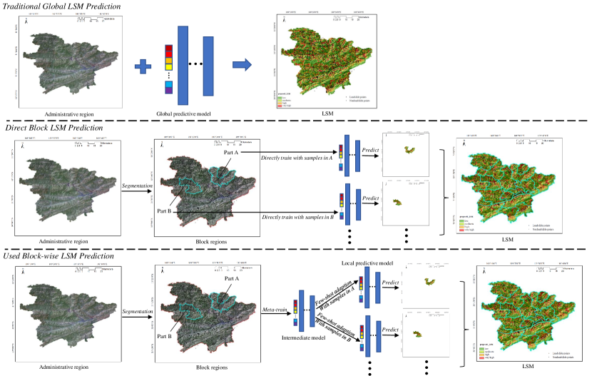
Figure 1: Three manners of predicting the LSM. Traditional global LSM prediction could lose veracity or even rationality in complex large scenarios with different landslide-inducing environments. When considering segmenting the scenarios for individual analysis, directly training predictive models for each block would suffer from having few available samples. Our method trains an intermediate model that can be quickly adapted to each block.

1.1 Limited generalization ability of a single model

Global analysis can elevate the fitting performance of a single model on given samples, but it limits the transferability of the model for being generalized to various scenarios. Because the landslide-inducing environments of various parts of a region may be different, it might be unreasonable to use only one model to represent multiple landslide causes. For example, suppose that the occurrence of a landslide in one region is extremely sensitive to the slope, while the occurrence in other regions is not. The model fed with similar input features should give the same output, but in this case, the occurrence of a landslide in two areas could be different states, that one input caused a landslide prediction, whereas the other did not. One possible reason is that the dominant causative factors, for example, lithology or rainfall, resulting in such discrepancy were not captured as feeding to the training model. Intuitively, to solve the generalization limitation, we divide the region into blocks and build models, respectively. We denoted this as block-wise analysis in this article.

1.2 Few samples for block-wise analysis

In large mountainous scenarios, access to landslide events is costly and limited. Because the collection of historical or assumptive landslide points requires not only expert knowledge but also involves an investigation of the probably dangerous site (Ciampalini et al., 2016). Therefore, the related issue is how the current model can be quickly adapted to unseen areas with only a few labeled samples. For this question, we considered whether there is an intermediate representation that is conditionally sensitive to variations in some aspects concerning general and vital landslide causes; thus, within these concepts, the representation could be few-shot adapted to new tasks.

1.3 Contribution

To solve the problems mentioned above, we proposed to decompose the global analysis into local analysis (whole study area into blocks, single task into multitasks), and meta-learns an intermediate representation that can be few-shot adapted to each task. The proposed pipeline contains unsupervised pretraining, scene segmentation and meta-task sampling, intermediate model meta-training, and few-shot adaption. Specifically, we first execute unsupervised pretraining with unlabeled samples to initialize the base model for subsequent meta-learning, with good properties, such as noise proof, disentangling correlated input features, stability to variations in training configuration, improving transferability of the base model, and embedding a more discriminative metric space. Then, to recast the global analysis and the model, we utilized a modified simple linear iterative clustering (SLIC) (Achanta et al., 2012) to effectively segment the large-scale scenario into superpixels for block-wise analysis. Finally, for the validity of applying meta-learner to solve the few-shot learning problem (Sung et al., 2018), we meta-learn an intermediate model so that local tasks in unseen areas could be quickly adapted. Meta-learning, as well as learning to learn, means learning concepts that can better or faster guide the model to learn desired representations. The intuition is that a more general representation is better suited for landslide susceptibility few-shot adaption.

The main contributions are listed as follows: (1) We propose a block-wise LSM approach to raise the veracity for modeling different parts of a scenario; and (2) more crucial is that we propose to meta-learn an intermediate representation that can be quickly adapted to unseen tasks with very few samples and gradient descent updates. It is feasible and efficient for large-scale LSM tasks where landslide records are limited. The remainder of this paper is organized as follows: In Section 2, related works are reviewed. In Section 3, the study area and dataset are introduced, while Section 4 presents the proposed method. Results and discussions are presented in Section 5, and section 6 concludes the paper.

2 Related works

This section reviews related statistical landslide susceptibility prediction methods and summarizes their characteristics.

Supervised Regression

Supervised regression refers to the prediction of the LSM with end-to-end nonlinear mapping trained by labeled samples (Chang et al., 2020). These methods are widely applied, for example, logistical regression (Chen et al., 2018), decision trees (Hong et al., 2020), support vector machines (Pham et al., 2019a), and evidential belief functions (Chen et al., 2019). Despite their outstanding performance in the face of simple scenarios, these models would lose veracity to fit the nonlinearity of complex landslide causes. To improve the representative power, researchers have either applied ensemble techniques (Hu et al., 2021) or increased the depth and width of the model. For example, in Pham et al. (2017), different base classifiers were combined, and in Wyner et al. (2017), an expanded multilayer perceptron (MLP) was applied, both to increase the precision of fitting the training data in a complex environment. The state-of-the-art random forest (RF) (Dou et al., 2019) is also regarded as a bagging method in ensemble techniques. Recently, convolutional neural networks (CNN) have also been applied for landslide susceptibility prediction (Fang et al., 2020; Yi et al., 2020). These methods are competent, but they can suffer from the deficiency of labeled samples to train large-capacity models in practice. In addition, poor quality of thematic information, such as non-uniform resolution, noise disturbance, the less rigorous feeding of correlated thematic features, and inaccurate supervision where labeled samples are not always the ground truth, would adversely impact predicting reasonable landslide susceptibility.

Unsupervised Representation Learning

Unsupervised learning takes a good insight into the unlabeled data structure and learns representations that are more suitable as a side effect for subsequent supervised learning (Amruthnath and Gupta, 2018) Some landslide susceptibility evaluations applied unsupervised representation learning before training the labeled samples. For example, Xu et al. (2015) used a sparse autoencoder to reduce redundancy and correlation in the conditioning factors and applied regularized greedy forests (Sameen et al., 2020) to predict landslide susceptibility with sparse representation. Wang et al. (2020) applied a deep belief network to disentangle independent concepts in a relatively low-dimensional space. Impressively, Zhu et al. (2020a) applied an adversarial manner to urge the model to learn a representation that shares as many underlying factors between source and target scenarios, which improved the transferability of the model to unseen areas. These unsupervised techniques open up a new way for potential hazard analysis. However, they neglect the irrationality to apply one global model to describe multi-environmental tasks and the very limited samples situation.

Meta Learning

Learning quickly from very few samples is a hallmark of human intelligence (Hospedales et al., 2020). For example, a child would recognize a horse picture based on the previous reading of an animal brochure. In contrast to the classifier trained with thousands of labeled samples, meta-learning aims to learn more general concepts among the tasks so that the desired model can be learned from only a few samples. Different from uninterpretable output trained by black-box supervised regression, it is worth researching if a landslide can also be quickly identified based on some meta-trained cognitive patterns. Model-agnostic meta-learning (MAML) (Finn et al., 2017) is a heuristic and typical work of meta-learning science, which innerly trains each meta-task and whose meta-objective is to minimize the sum of losses from related tasks. To generalize the ideology of meta-training, Metz et al. (2018) introduced an unsupervised weight update rule that applies an MLP for hyperparameter meta-training. Despite its superiority, few studies have discussed the potential and advantages of applying meta-learning techniques to solve the problems above in LSM prediction. In this study, we explored the superiority of meta-learning in capturing general concepts from LSM tasks and tested the few-shot adaption and generalization performance.

3 Study areas and datasets

There were two study areas (Fig. 2), the Fengjie County (FJ) and Fuling District (FL), both located in Chongqing City, China. Chongqing City is the largest city in China and features mountainous areas with complex landslide-inducing environments. In the past, many devastating landslide events have occurred, for example, the typical Tangjiewan, Xinmo, and Mabian landslides (Fan et al., 2018; Scaringi et al., 2018; Wei et al., 2019).

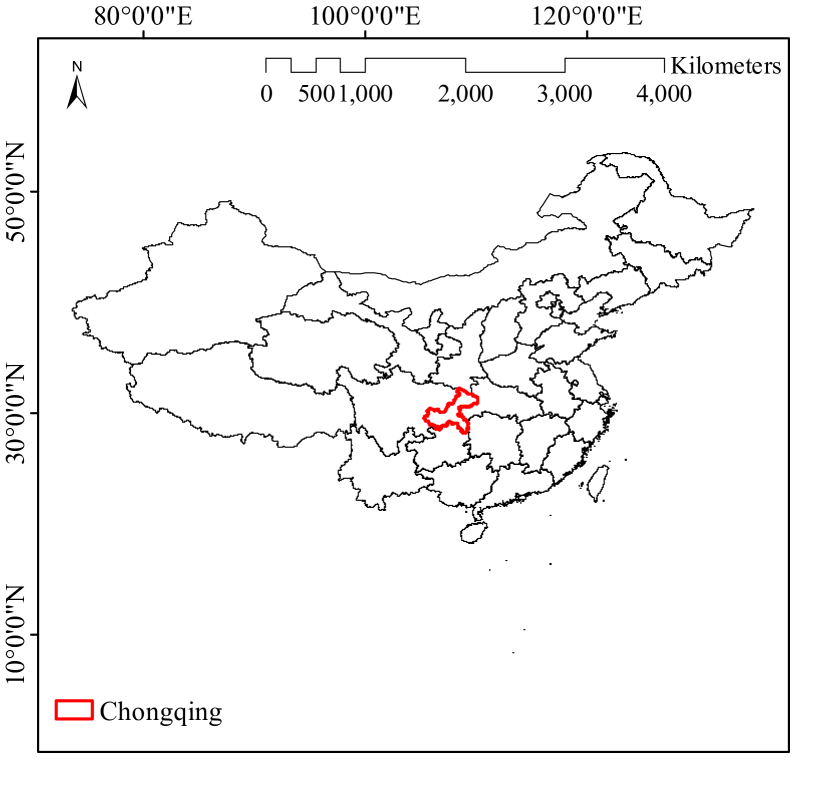
(a) Administrative districts of China

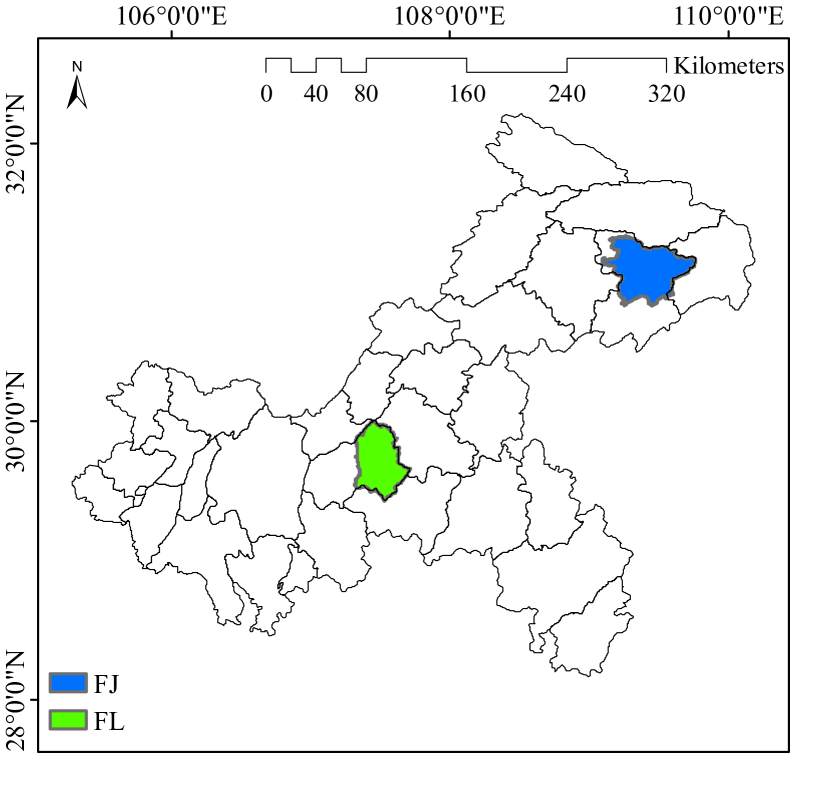
(b) Chongqing City

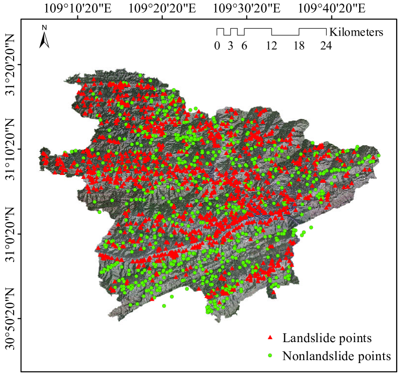
(c) Fengjie County (FJ)

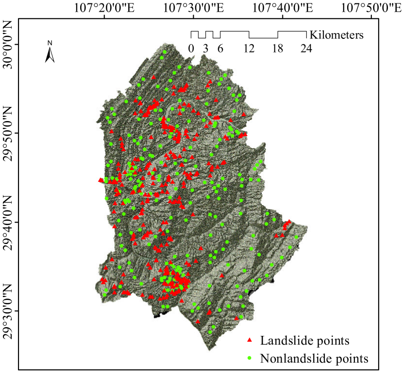
(d) Fuling District (FL)

Figure 2: Location of the two study areas FJ and FL: (a) administrative map of China and the location of Chongqing City; (b)admistrative map of Chongqing City and the locations of FJ and FL; (c) (non)landslide distribution in FJ and FL.

The landslide inventory was collected from the Chongqing Geomatics and Remote Sensing Center. In addition to historical landslide records, potential landslide locations inferred by expert knowledge and on-site investigation were also collected. There were approximately 1200 available landslide records in FJ, and approximately 400 landslide records for FL, as positive samples. We randomly selected the same amount of non-landslide points as the negative samples.

The thematic maps related to landslide susceptibility analysis were downloaded from online platforms Computer Network Information Center (CNIC), Chinese Academy of Science, and U.S. Geological Survey (USGS) (CNIC, 2021; USGS, 2021). According to Jebur et al. (2014), the thematic maps used to feature an input sample vector in this study consisted of landslide occurrence frequency, strata type, digital elevation model (DEM), aspect, slope, curvature, normalized difference vegetation index (NDVI), vegetation coverage, soil erodibility, sand coverage, clay coverage, silt coverage, topographic wetness index (TWI), stream power index (SPI), distance to drainage, and distance to the road. Each thematic map is thought to contain some aspects possibly related to the occurrence of a landslide. The thematic maps of FJ and FL are shown in Fig. 3 and Fig. 4, respectively, together with the distribution of the landslide locations. The sampling method for each landslide record of this article refers to Zhu et al. (2020a). It is worth mentioning that different thematic maps have different resolutions, but it does not affect the sampling process. Our method dealt directly with the original numerical values featured in the thematic maps. Further, to avoid numerical problems, all sample vector dimensions were normalized (Sun et al., 2021).

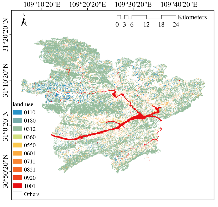
(a) land use

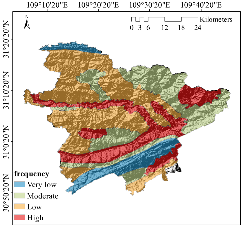
(b) frequency

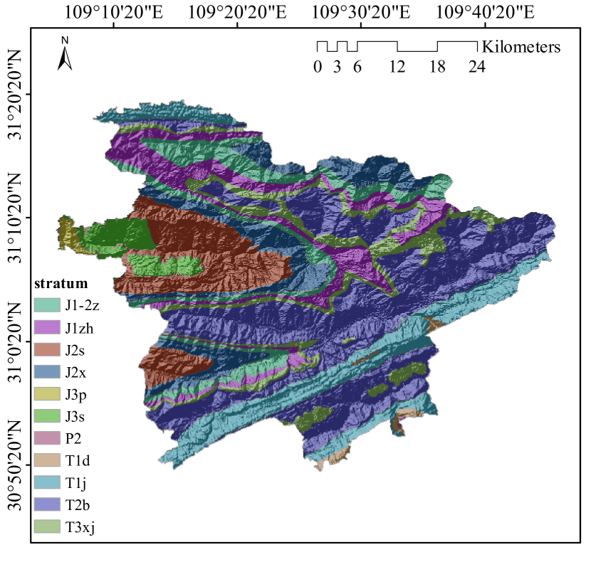
(c) strata type

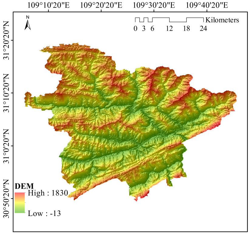
(d) DEM

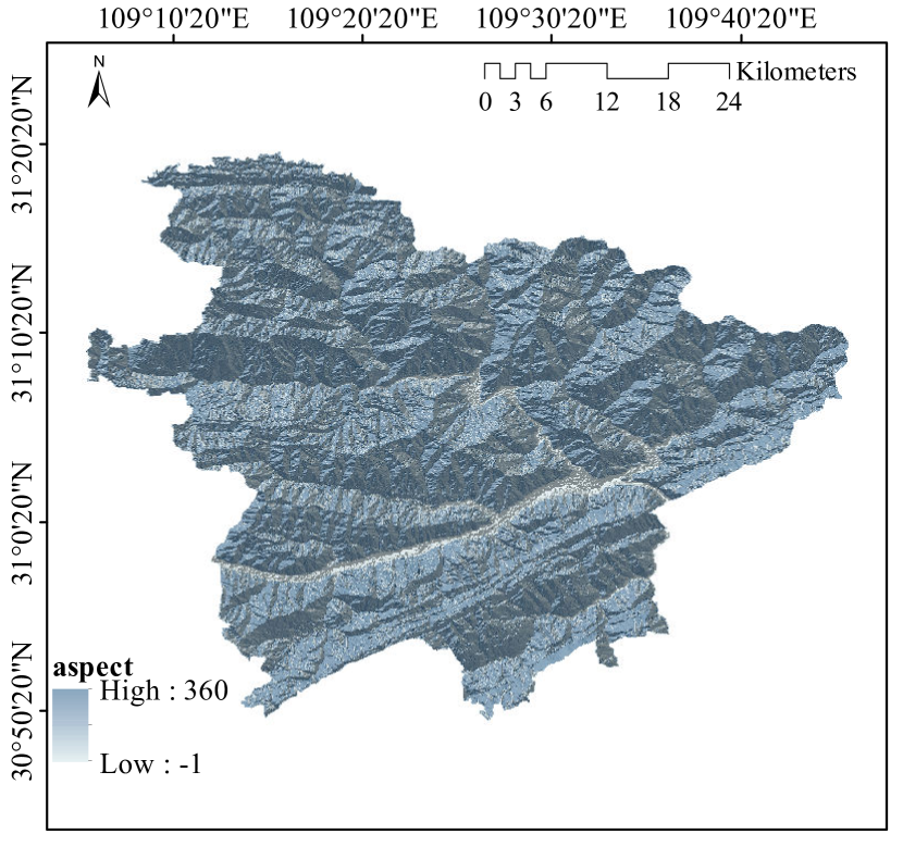
(e) aspect

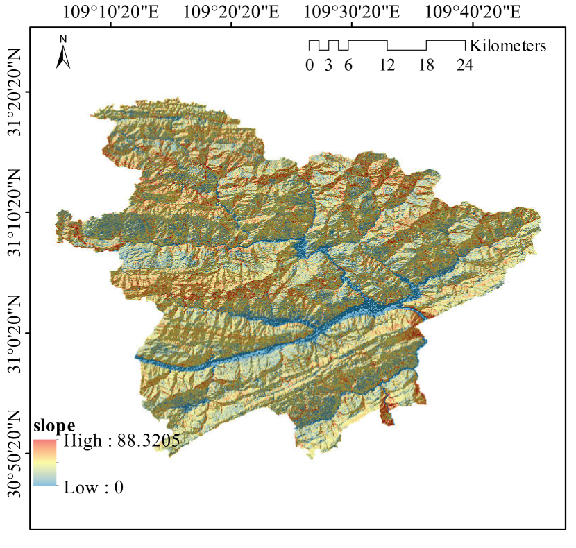
(f) slope

(g) curvature

(h) NDVI

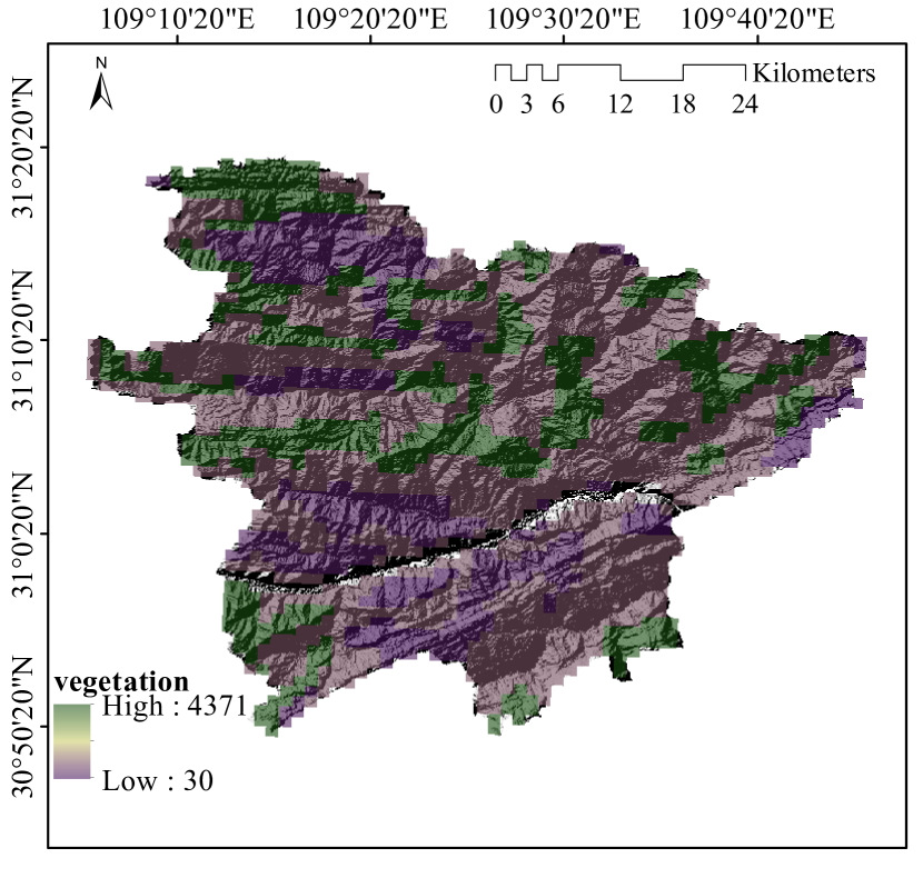
(i) vegetation coverage

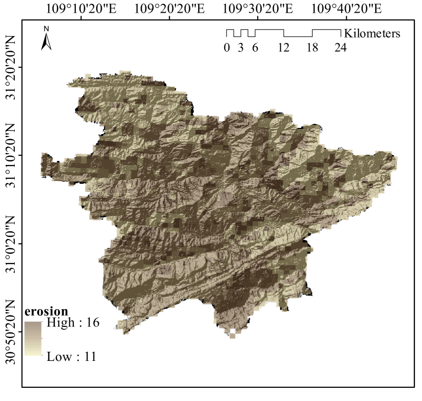
(j) soil erodibility

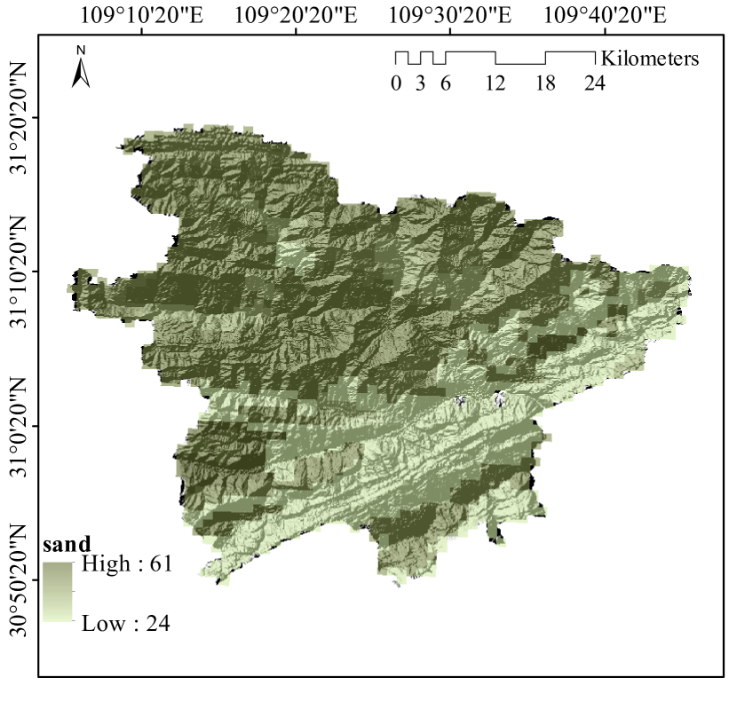
(k) sand coverage

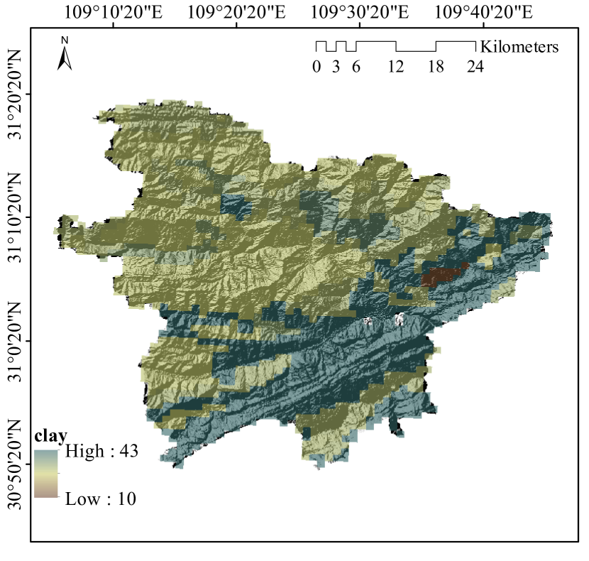
(l) clay coverage

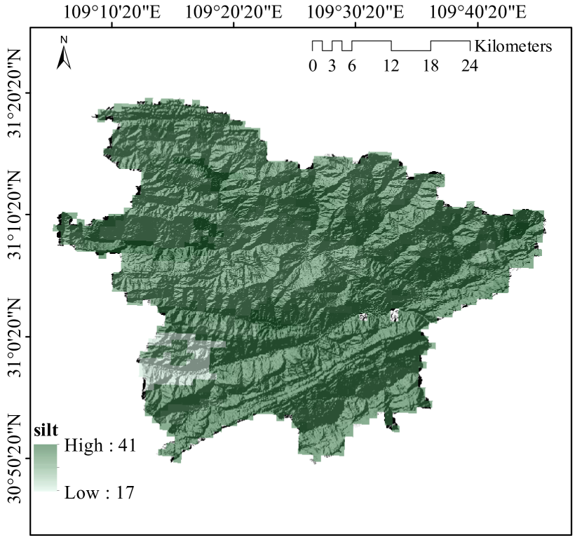
(m) silt coverage

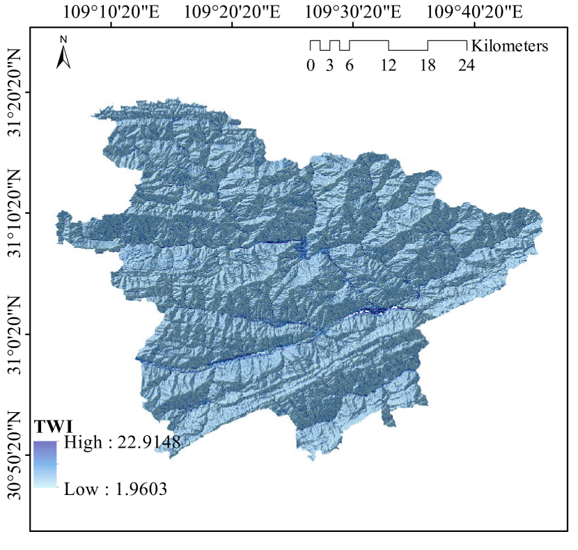
(n) TWI

(o) SPI

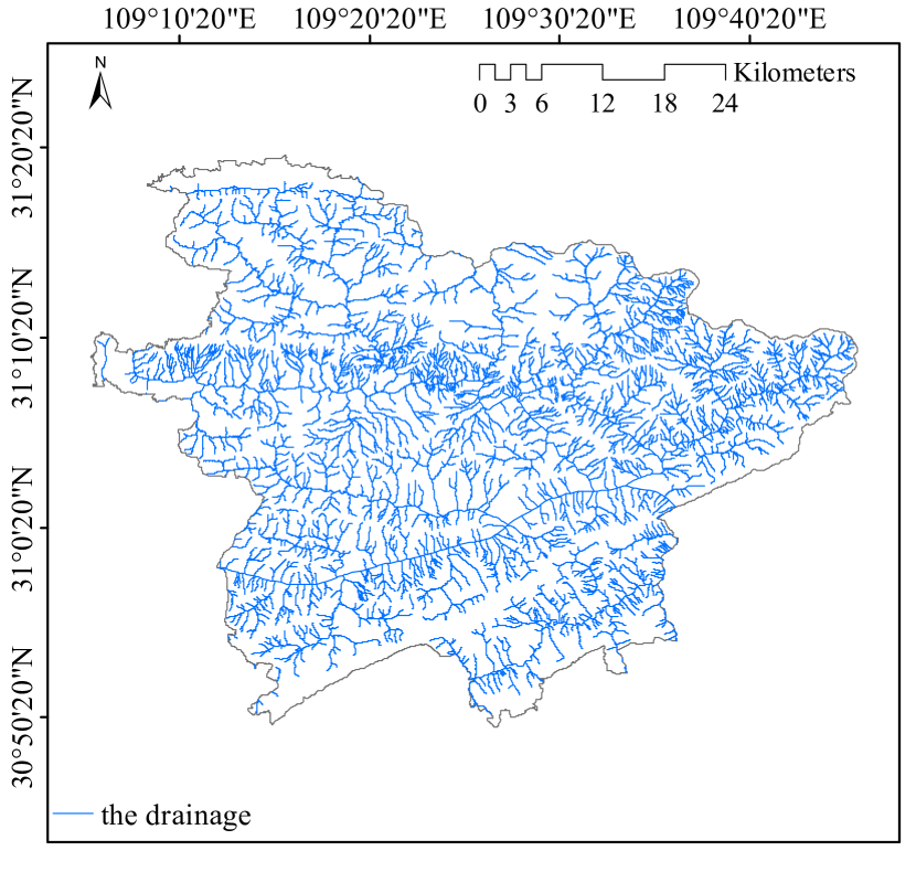
(p) drainage

Figure 3: Thematic maps of Fengjie County. (a) Land use, (b) landslide occurrence frequency, (c) strata type, (d) DEM, (e) aspect, (f) slope, (g) curvature, (h) NDVI, (i) vegetation coverage, (j) soil erodibility, (k)sand coverage, (l) clay coverage, (m) silt coverage, (n) TWI, (o) SPI, and (p) drainage.

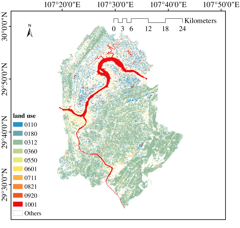
(a) land use

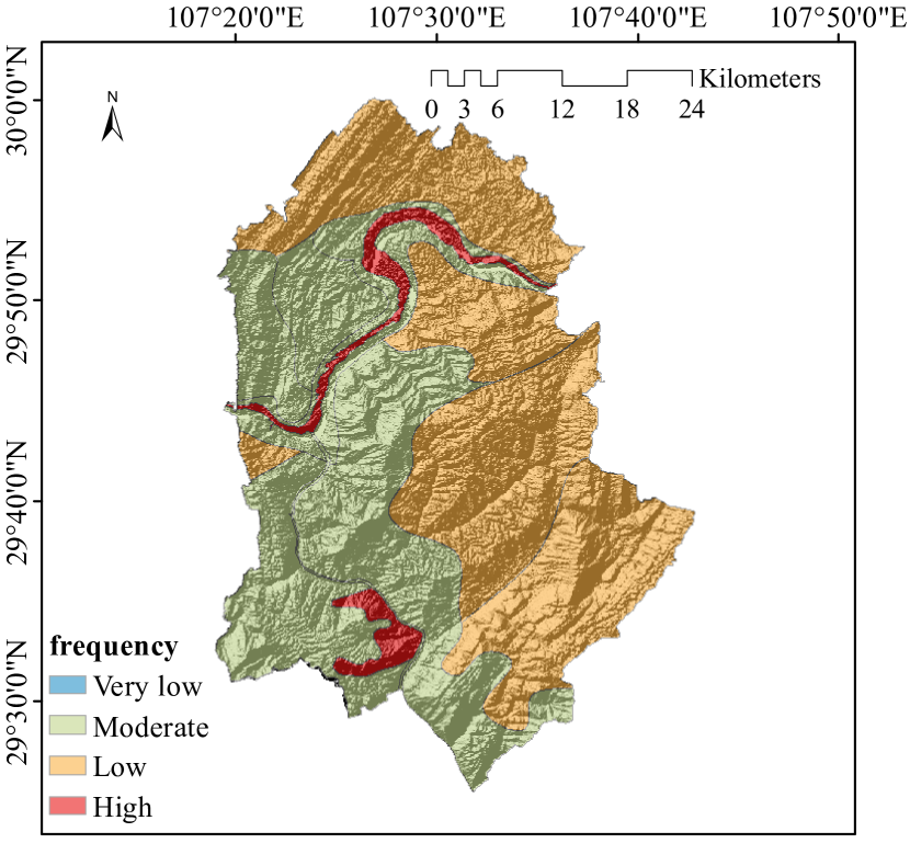
(b) frequency

(c) strata type

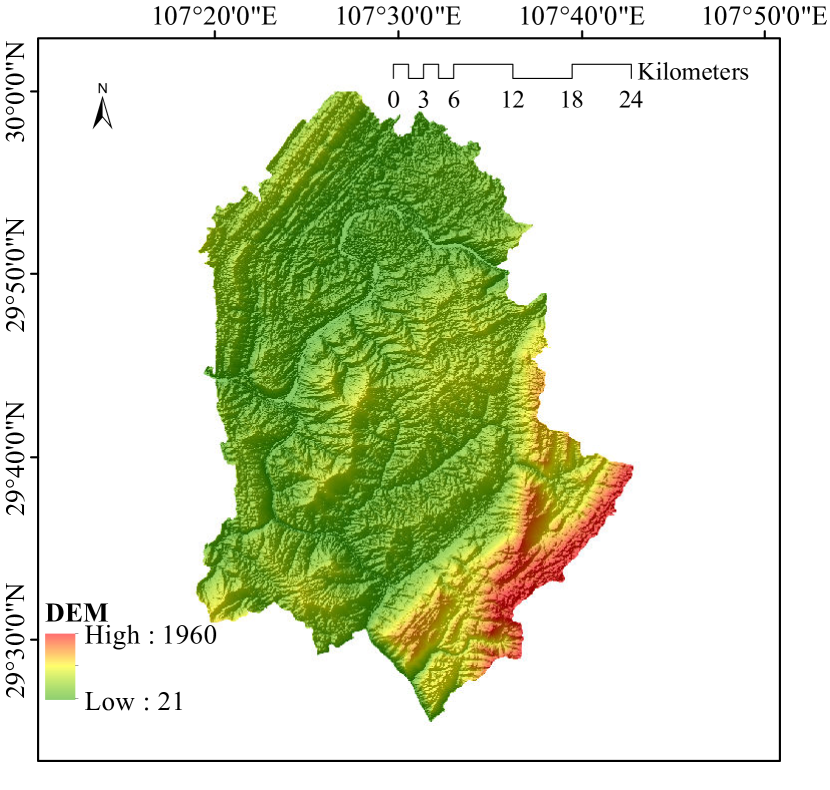
(d) DEM

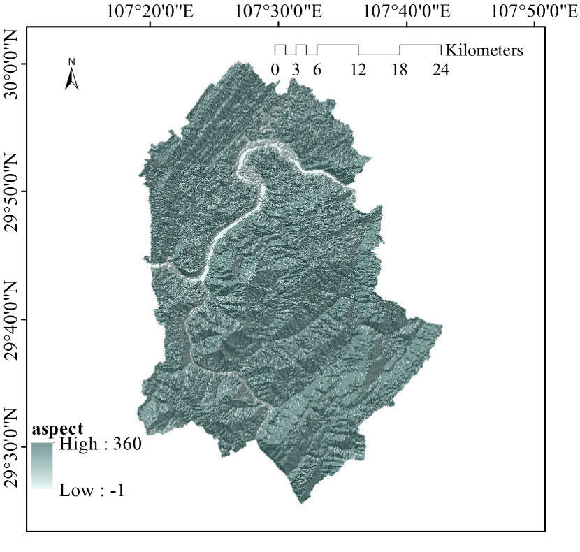
(e) aspect

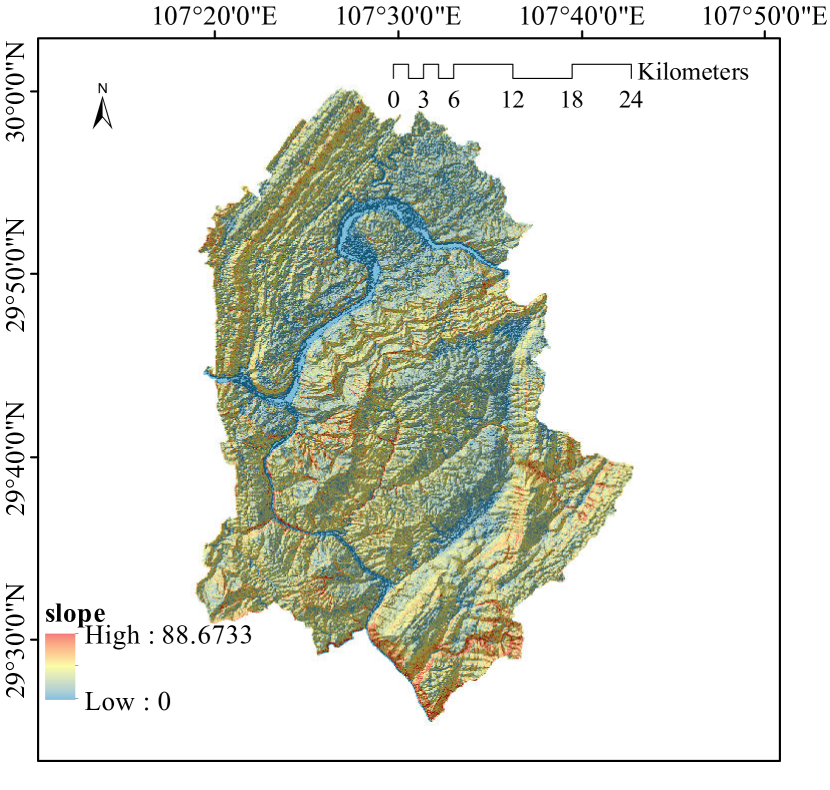
(f) slope

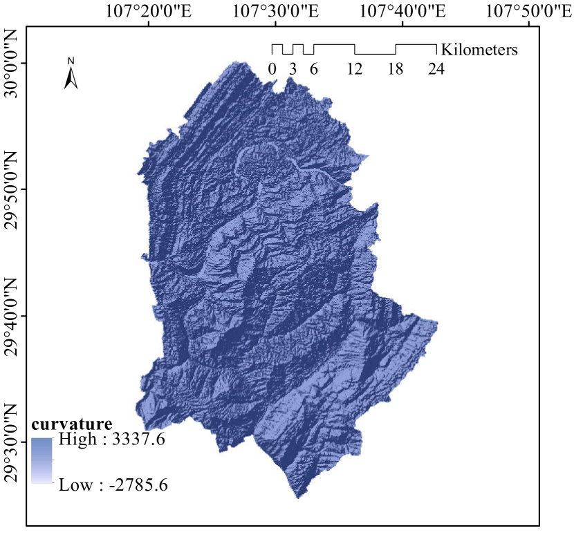
(g) curvature

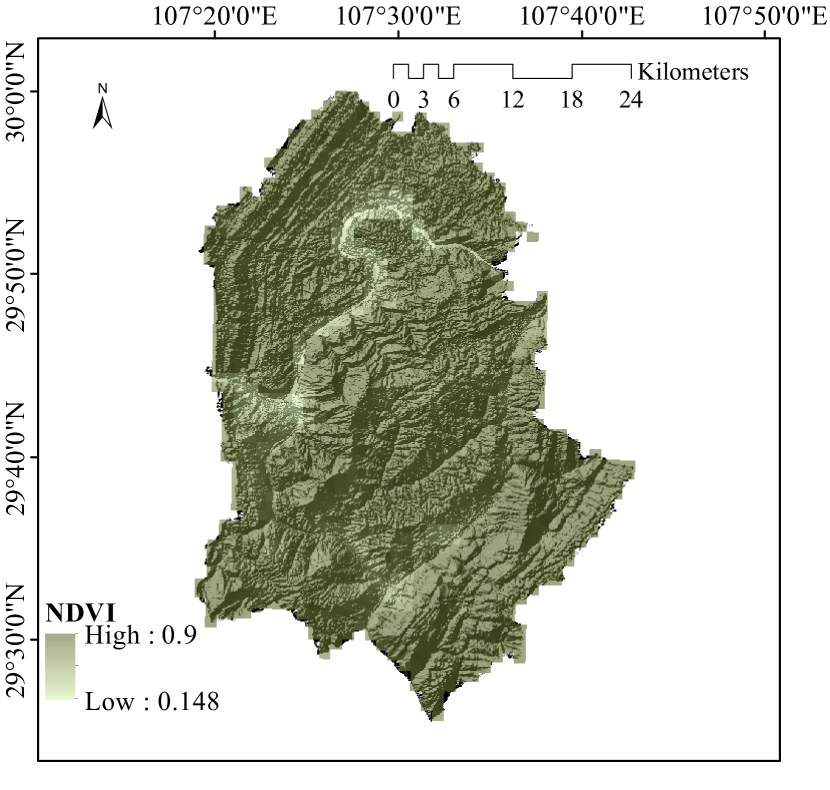
(h) NDVI

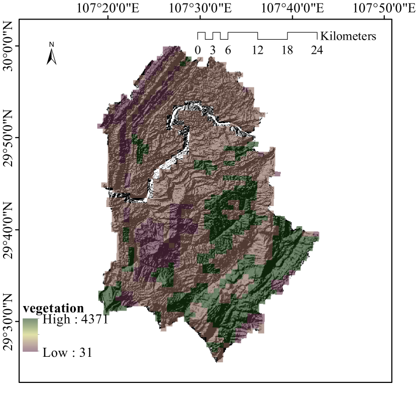
(i) vegetation coverage

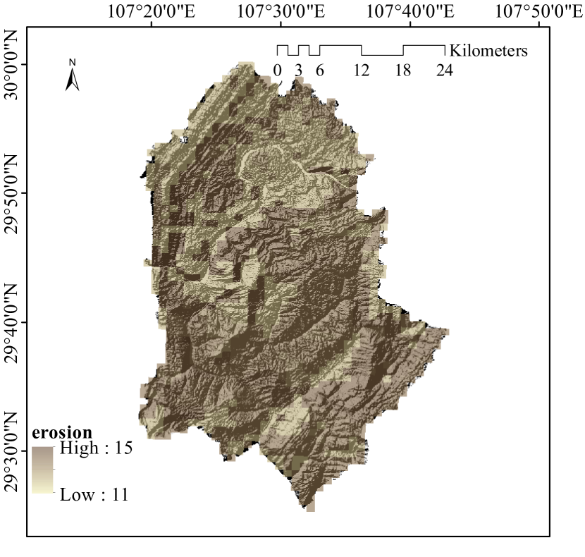
(j) soil erodibility

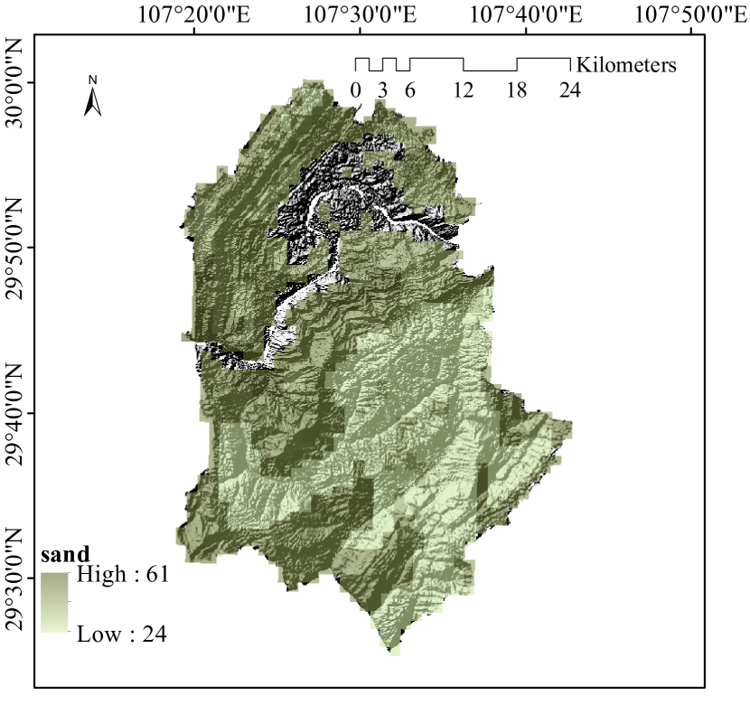
(k) sand coverage

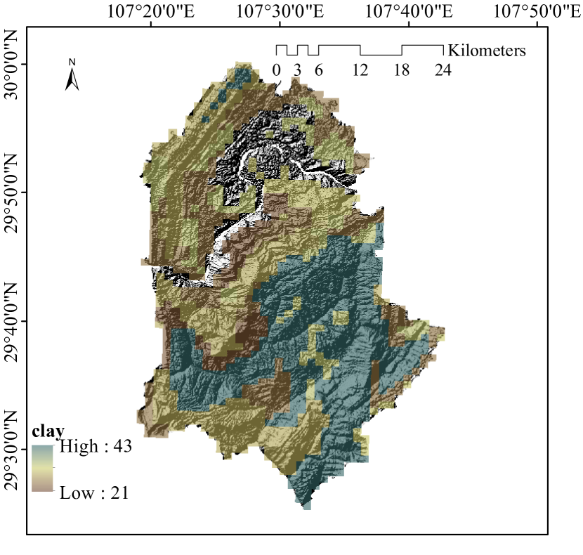
(l) clay coverage

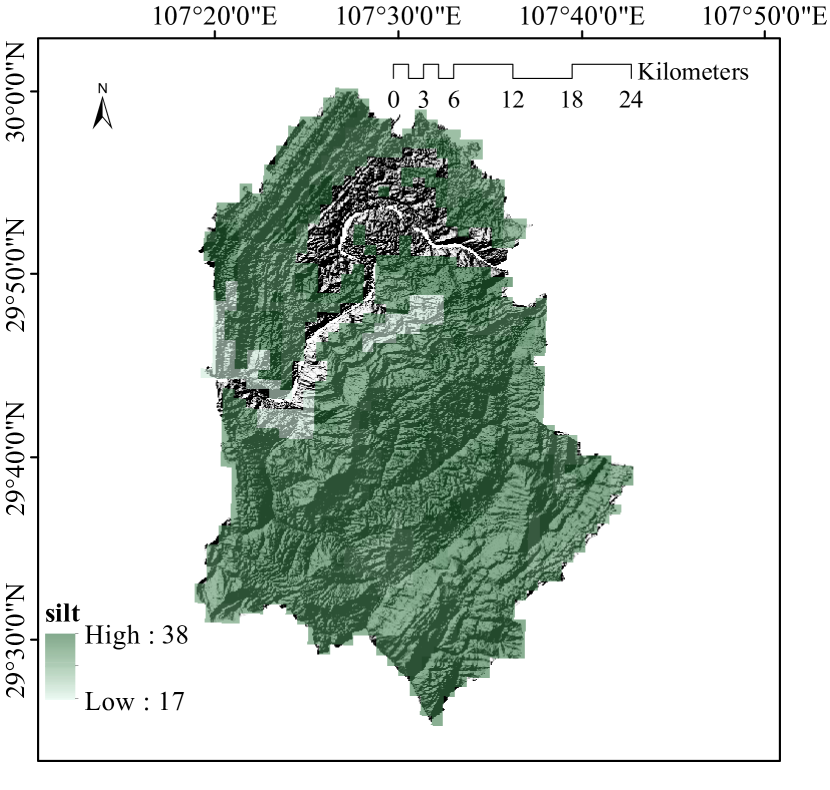
(m) silt coverage

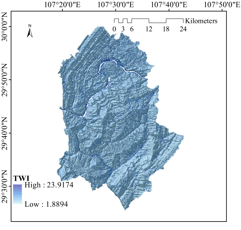
(n) TWI

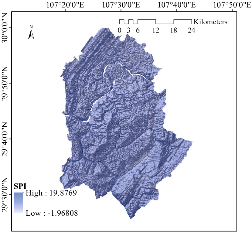
(o) SPI

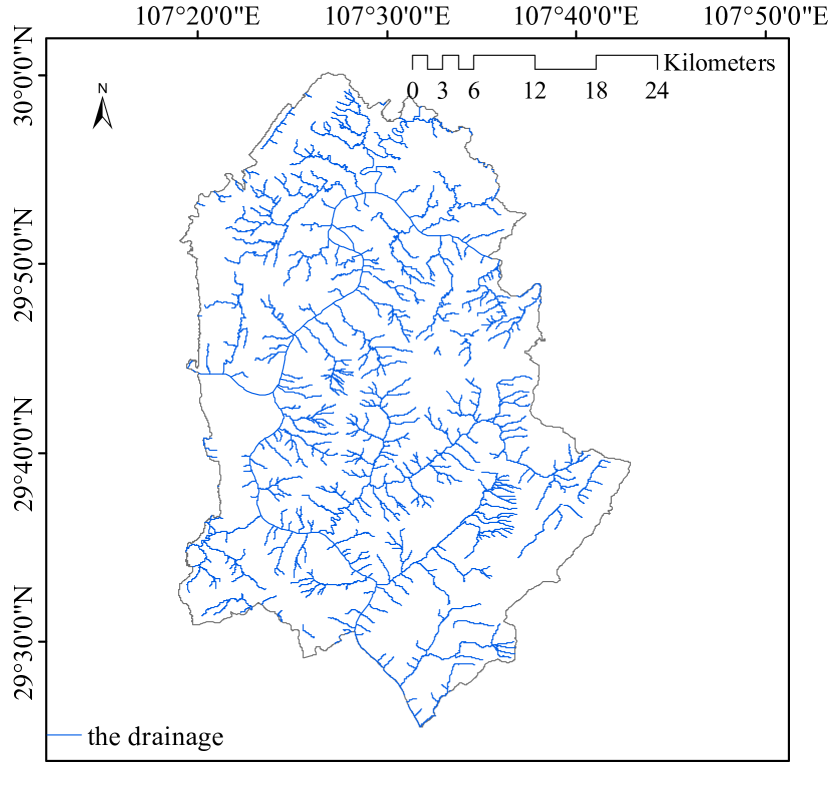
(p) drainage

Figure 4: Thematic maps of Fuling District. (a) land use, (b) landslide occurrence frequency, (c) strata type, (d) DEM, (e) aspect, (f) slope, (g) curvature, (h) NDVI, (i) vegetation coverage, (j) soil erodibility, (k) sand coverage, (l) clay coverage, (m) silt coverage, (n) TWI, (o) SPI, and (p) drainage.

4 Proposed method

4.1 Overview and problem setup

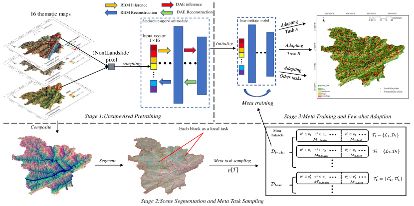
Figure 5: Overview of the proposed method. Our method contains an unsupervised pretraining stage for learning superior representations with good properties; a scene segmentation and task sampling stage for producing meta-datasets; and the meta-training stage for learning intermediate model suited for few-shot adaption of block-wise LSM prediction, which is further explained in Section 4.4.

4.1.1 Overview of the methods

The global prediction of the LSM would lose veracity and even rationality in circumstances where various parts of the target region hold different landslide-inducing environments. Thus, we used multiple models to learn the LSM predictive model for different parts of the region. Based on this, however, the model of each part of the region would be vulnerable to very few labeled samples. To solve this problem, we introduced meta-learning technology for few-shot adaption (Ren et al., 2018). An overview of the proposed method is presented in Fig. 5, containing three steps: (1) unsupervised pretraining to transform original data into embedding space with good properties; (2) scene segmentation for local task sampling to generate meta-datasets; (3) and meta-training to obtain an intermediate representation that is suited for few-shot adaption to unseen tasks.

4.1.2 Problem setup

Formally, the initial inputs consist of $M$ thematic maps $\varGamma\{\varGamma_{1},...,\varGamma_{M}\}$ and $N$ landslide (and non-landslide) samples $\mathcal{S}\in\mathbb{Z}^{2\times N}$ with latitude and longitude information within the World Geodetic System. Each sample $s_{i}$ in $\mathcal{S}\in\mathbb{Z}^{2\times N}$ features from $\varGamma$ such that sample vectors $\mathcal{V}\in\mathbb{Z}^{M\times N}$ are generated. Within our framework, $\mathcal{V}$ is first fed as unlabeled samples into the unsupervised pretraining stage to initialize the base model, denoted $f$, which maps input features to output representation $f_{0}$. After the initialization, we apply SLIC (Achanta et al., 2012) to segment the target scenarios into blocks $\mathcal{B}\{b_{1},...,b_{K}\}$, and then divide the vectors $\mathcal{V}$, labeled as $\mathcal{V}_{l}\{v_{1},...,v_{K}\}$, according to their location in $\mathcal{B}$, thus building meta-task distribution $\mathcal{T}_{k}\{\mathcal{L}_{k},\mathcal{D}_{k}\}\sim p(\mathcal{T})$. $\mathcal{L}_{k}$ is the inner loop loss function, and $\mathcal{D}_{k}$ is the meta-datasets. The purpose is then to meta-learn an intermediate model $f^{\prime}$ that can be adapted to unseen tasks $\mathcal{T^{\prime}}_{k}$, which is further discussed in Section 4.4. Next, we fine-tune $f^{\prime}$ with $v_{i}\in\mathcal{V}_{l}$ to obtain the adapted model $f^{\prime}_{i}$ for each block $b_{i}\in\mathcal{B}$. Finally, we use $f^{\prime}_{i}$ to predict the LSM of the region associated with $b_{i}\in\mathcal{B}$.

4.2 Representation learning for initialization of meta-learner

Despite the convenience to be available to online data, several problems remain, for example, (1) data are generally noisy with various resolutions, owing to the high cost of access to high-quality thematic information of large-scale areas; (2) inducing factors inferred from thematic maps can be correlated and explain the same aspect of the occurrence of a landslide; and (3) unreasonable selection of thematic information would be expected to lead to redundant or confusing conceptions for supervised regression.

The first stage of the proposed method serves as a pretraining process to train the base model of the meta-learner with unlabeled samples for learning the representation $f_{0}$ featuring robustness, independence, and compactness. Specifically, the model is composed of sequential stacked unsupervised learning modules, which include two restricted Boltzmann machines (RBMs) (Nair and Hinton, 2010) and a denoising autoencoder (DAE) (Vincent et al., 2008). Regarding the RBM, the objective is to minimize the Kullback-Leibler divergence (Hinton, 2002) between a given sample distribution and the distribution inferred from the model. The essential problem in the objective is to calculate the two intractable expectations in Eq. 1,

$$\begin{split}\frac{\partial{lnP{v^{i}}}}{\partial\theta}&=\mathbb{E}_{P_{data}}[\cdot]+\mathbb{E}_{P_{model}}[\cdot]\end{split}$$ (1)

where $P{v^{i}}$ is the probability of the $i$th sample vector $v^{i}\in\mathcal{V}$, $\mathbb{E}_{P_{data}}[\cdot]$, and $\mathbb{E}_{P_{model}}[\cdot]$ denote data-dependent expectation and model’s expectation. A standard method is to approximate the intractable expectation $\sum_{v}[\cdot]$ using Gibbs sampling (Nair and Hinton, 2010), which describes the Markov process carrying out many state transfers between visible and hidden states to approach the stationary distribution represented by the model. Nevertheless, a stochastic state still requires too many cycles to reach Gibbs distribution. Aiming to improve the learning efficiency, Hinton (2002) proposed Contrastive Divergence (CD-k algorithm), in which data sample is used as initial visible state and proved that by just applying $k$ ($k=1$ usually) step(s) Gibbs sampling, we could sufficiently approach the distribution that the model represents. Regarding the DAE, the objective is to minimize the reconstruction error between the corrupted input and the reconstructed representation (Vincent et al., 2008).

The unsupervised training strategy follows the greedy layerwise pretraining rule in Salakhutdinov and Hinton (2009) to train unsupervised modules sequentially. We were based on the premise of RBM that the hidden units are conditionally independent of each other (Hinton, 2007), thus disentangling correlated input units and making the hidden space more discriminative. We applied DAE to enhance the noise-proof of the model and compress the output representation. The stacked modules will enhance the representative power of the model to fit complex tasks. Futhermore, we increased hidden units to generate more independent and descriptive hidden units, which borrows the part of thought in the $1\times 1$ convolution (Lin et al., 2013).

4.3 Scene segmentation and meta-task sampling

The global analysis will build a reasonable predictive model if there are plenty of landslide/non-landslide points within a single scene, where most landslides occurred for the same causes. However, in most cases, especially for the large-scale scenario, the causes of a landslide in each part of that scenario are pretty different. Accordingly, we segmented the scenario into several parts and modeled them respectively.

4.3.1 Scene segmentation using combined feature and spatial distance

The segmentation approach is based on simple linear iterative clustering (SLIC) (Achanta et al., 2012) for its simplicity and efficiency. It is superior when processing large-scale areas. The collected thematic maps $\varGamma=\{\varGamma_{1},...,\varGamma_{M}\}$ are first clipped with the study areas and then merged into a composition. Next, according to the input parameters $K$, which denotes the number of output superpixels (blocks), the study area is evenly divided into $K$ grids $\mathcal{B}\{b_{1},...,b_{K}\}$ with a size of $S=\sqrt{N/K}$, where $N$ denotes the number of pixels within the study area. The cluster center $C_{k}$ of each block $b_{K}$ is then initialized by the grid center with features $ft_{k}(z_{1},...,z_{M})$ and position ($x_{k}$, $y_{k}$). To refine this rough initialization for the subsequent pixel assignment process, we move the cluster centers to the lowest gradient position in a $5\times 5$ neighborhood, in case the cluster centers lie on the edge of the scene or noisy pixels, which could cause a negative effect when calculating the distance measure $D$, $D$ is given as in Eq. 2:

$$\begin{split}\begin{aligned} d_{f}&=\|ft_{j}(w_{1}z_{1},w_{2}z_{2},...)-ft_{i}(w_{1}z_{1},w_{2}z_{2},...)\|^{2},\\ d_{s}&=\sqrt{(x_{j}-x_{i})^{2}+(y_{j}-y_{i})^{2}},\\ D&=\sqrt{d_{f}^{2}+(\frac{d_{s}}{S})^{2}M^{2}},\end{aligned}\end{split}$$ (2)

where $d_{f}$ is the feature distance, $x_{k}$ is the $k$th dimension of $f$, $w_{k}$ is the weighting value of the $i$th dimension, $d_{s}$ is the spatial distance, and $M$ weights the relative importance between feature similarity and spatial proximity. Notice that inducing factors could exert different levels of contribution to the occurrence of a landslide. Thus, each considered feature $x_{m}$ is weighted with $w_{m}$ based on (Popescu, 2002) in this study.

In the pixel assignment process, for each pixel $P_{i}$, the corresponding sample vector $v_{i}\in\mathcal{V}_{l}$ is located in, $l_{i}$ is initialized as -1 and $d_{i}$ as $\infty$, where $l_{i}$ denotes which block $b_{i}$ is the pixel belonging to, and $d_{i}$ denotes the closest distance from a superpixel center $C_{k}$ to that pixel. Next, we search in a $2S\times 2S$ region around the cluster center $C_{k^{\prime}}$ to identify the pixels that have the closest distance $D_{min}$ to that center compared to others. Then, we assign $l_{i}$ with $k^{\prime}$, $d_{i}$ with $D_{min}$. Once the assignment is completed, labeled sample vectors are grouped into $\mathcal{V}_{l}\{v_{1},...,v_{K}\}$ by $l_{i}$.

4.3.2 Meta-task generation

After the scene segmentation process, $\mathcal{B}\{b_{1},...,b_{K}\}$ is used for meta-task sampling $\mathcal{T}_{k}\sim p(\mathcal{T})$. Specifically, each segmented superpixel is simply regarded as a task scenario $\mathcal{T}_{k}=\{\mathcal{L}_{k},\mathcal{D}_{k}\}$, where $\mathcal{L}_{k}$ is the inner loop loss function and $\mathcal{D}_{k}$ is the collection of sample vectors $v_{i}\in\mathcal{V}_{label}$ of $\mathcal{T}_{k}$. From these meta-datasets, we randomly choose 60% of $\mathcal{D}$ as the training set $\mathcal{D}_{train}$ for meta-training, and the other as the testing set $\mathcal{D}_{test}$ for validation. For each task $\mathcal{T}_{k}$ in $\mathcal{D}_{train}$, $\mathcal{D}_{k}$ is divided into a training part $\mathcal{M}_{k\_train}$ (also known as the support set), and a testing part $\mathcal{M}_{k\_test}$ (also known as the query set) serving separately for the inner and outer loop optimization. The meta-datasets are organized as in Fig. 5. $\mathcal{D}_{k}$ has only a few samples.

4.4 The meta-learner

In particular, utilizing only one predictive model can lose veracity when large-scale scenarios consist of districts with various landslide-inducing environments. In addition, the traditional data-driven method is vulnerable to the deficiency of high-quality thematic information and historical landslide records because of the vast costs of data collection. As a resolution, the meta-learner, shown in Fig. 6, is designed for learning a general intermediate model for few shot adaption. The meta-learning strategy consists of two levels of loops of computation (Goldblum et al., 2020), an inner loop for the optimization process, and an outer loop for optimizing some aspects of the inner loop, for example, the hyperparameters or even the optimization manner.

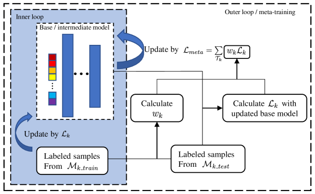
Figure 6: The meta-learner.

Formally, concerning the inner loop, suppose that we have constructed a model parameterized with $\theta$ that is initialized by $f_{0}$, pre-trained in Section 4.2, we use $\mathcal{M}_{k\_train}$ in $\mathcal{D}_{k}$ to train the model with few gradient descent updates by $\mathcal{L}_{k}$. Eq. 3 gives the optimization,

$$\begin{split}\theta_{k}^{{}^{\prime}}=\theta-\alpha\nabla_{\theta}\mathcal{L}_{k},\end{split}$$ (3)

where $\theta_{k}^{{}^{\prime}}$ denotes the updated parameter, which can be represented by $\theta$, $\alpha$ denotes the inner learning rate, and we choose cross entropy as $\mathcal{L}_{k}$, as given in Eq. 4,

$$\begin{split}\mathcal{L}_{k}=\frac{1}{N}\sum\limits_{k}-[y_{k}\cdot log(p_{k})+(1-y_{k})\cdot log(1-p_{k})],\end{split}$$ (4)

where $y_{k}$ denotes the label of the $k$th sample, $p_{k}$ represents the probability that the $k$th sample is predicted to be positive.

With such few samples and training steps, the meta-objective is then to minimize the sum of test errors of tasks in $\mathcal{D}_{train}$, which urges the model to excavate the conception sensitive to task variations so that a few samples and iterations could make large improvements to new task adaption. For this study, we consider the circumstances of inaccurate supervision, where the given landslide labels are not always the ground truth, which could cause highly adverse effects on meta-learning because only very few samples are used in the inner optimization or model fine-tuning (Hoffmann et al., 2011). In other words, the losses computed from wrong labels could account for a large proportion of the task loss $\mathcal{L}_{k}$, thus misleading the gradient in the descending direction. To alleviate the adverse effect, we introduce a method of weighting $\mathcal{L}_{k}$ to restrain tasks with very few samples, assuming that it is more likely to neutralize the wrong loss in a task with relatively more samples. Accordingly, the meta-objective $\mathcal{L}_{meta}$ is given by Eq. 5,

$$\begin{split}\mathcal{L}_{meta}=min\sum\limits_{\mathcal{T}_{k}\sim p(\mathcal{T})}w_{k}\mathcal{L}_{k},\end{split}$$ (5)

where $w_{k}$ is the weight of $\mathcal{T}_{k}$. This promotes the stability and reliability of training an intermediate model, which is further discussed in Section 5.3. In this study, during the iteration when generating the task batch, $w_{k}$ of task $\mathcal{L}_{k}$ is given by Eq. 6,

$$\begin{split}w_{k}=\frac{exp(n^{k}/n_{total})}{\sum\limits_{i}exp(n^{i}/n_{total})},\end{split}$$ (6)

where $n_{total}$ is the number of total samples in FJ and FL, $n^{k}$ is the number of samples in $\mathcal{T}_{k}$, and $i$ denotes the index of the task in a meta-training batch.

4.5 Few-shot adaption and block-wise LSM prediction

Once the intermediate model $f^{\prime}$ is meta-trained, the few-shot adaption or validation process for $\mathcal{T}_{k}$ and $\mathcal{T^{\prime}}_{k}$ simply repeats the optimization in Eq. 3, using sample vectors $\mathcal{M}_{k\_train}$ and $\mathcal{M^{\prime}}_{k\_train}$, and with very few iterations. Thus, we obtain adapted model $f^{\prime}_{i}$ for each block $b_{i}\in\mathcal{B}$. We then rasterize the FJ and FL areas and feature grids within each block $b_{i}$ into $g_{i}\in G\{g_{1},...,g_{K}\}$ by means introduced in Section 3. Next, for each block $b_{i}$, we match corresponding predictive model $f^{\prime}_{i}$ to predict the landslide susceptibility of $g_{i}$. Finally, we integrate $G\{g_{1},...,g_{K}\}$ and output the landslide susceptibility map. The intermediate model $f^{\prime}$ is meta-trained together with FJ and FL tasks, such that more general concepts can be learned from various landslide-inducing environments.

4.6 Implement details

The proposed method was implemented based on the tensorflow framework (version Tensorflow-gpu 1.9.0). In the stage of initializing the meta learner (unsupervised pretraining stage), RBMs and DAE were trained sequentially by the Adam optimizer from the bottom to top, with learning rates of 1e-3 and 1e-5, respectively. Both training epochs were set to 20. In the scene segmentation stage, limited to the number of samples, $K$ of FL and FJ were set to 196 and 64, respectively. The iteration loop of the pixel assignment process was set to 5. In the meta-learning stage, we initialized the inner learning rate $\alpha$ as 1e-1, which was relatively large and suited for quick adaption. The numbers of iterations of the inner optimization and few-shot adaption were both set to 5. The epoch of training meta-objective was set to 5000 with a learning rate of 1e-4. The code and data were made publicly available on the website.

5 Results and discussion

In this section, we first predict landslide susceptibility and evaluate the performance. Then, we analyze the effect of unsupervised pretraining and how our meta-learner weakens the adverse effects of inaccurate supervision and realizes faster adaption to new unseen local tasks.

5.1 Evaluation and comparison

5.1.1 LSM predction results

We compare our method with MLP-based (Zare et al., 2013), state-of-the-art RF-based (Catani et al., 2013), and an unsupervised representation-learning-based (RL-based) (Zhu et al., 2020a) approaches. In addition, to further demonstrate the validity of the proposed method, we compare it with the typical few-shot learning approach MAML (Finn et al., 2017). Fig. 7 and Fig. 8 depict the LSMs of FJ and FL by different approaches. There are four levels of susceptibility separated by predictive value, with a nearly equal number of raster samples in each susceptibility range, for intuitive comparison.

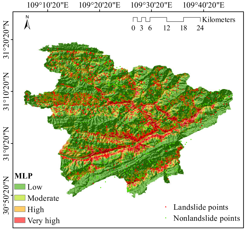
(a) MLP-based

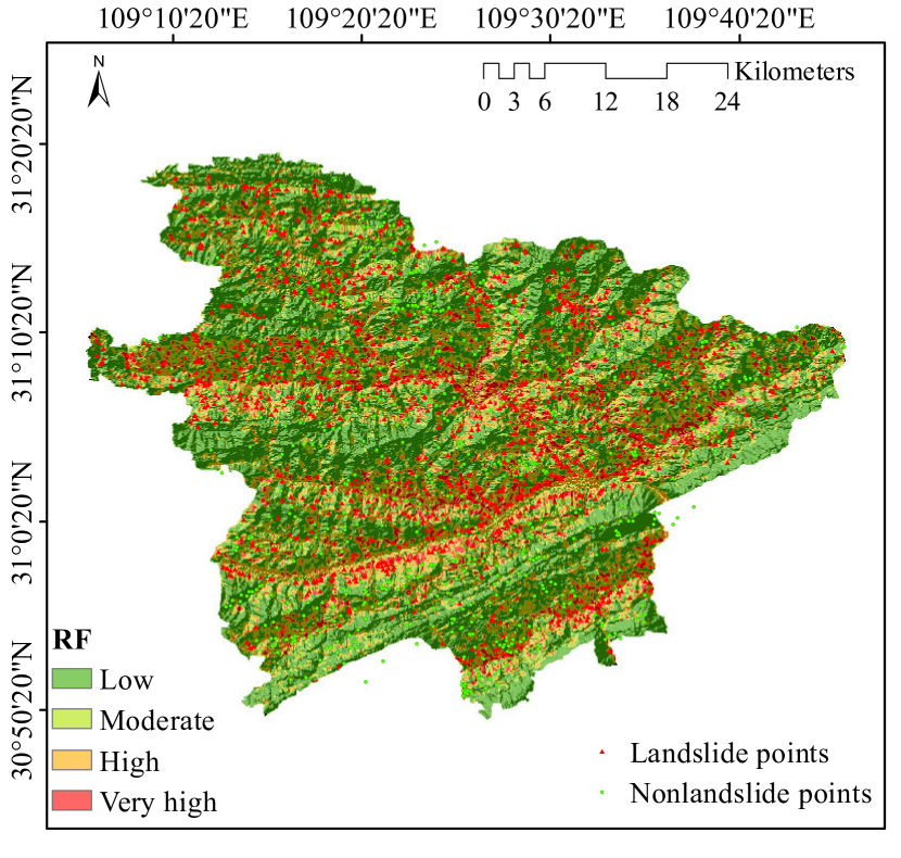
(b) RF-based

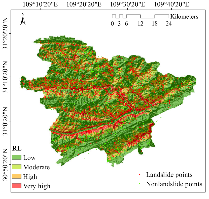
(c) RL-based

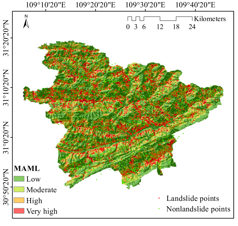
(d) MAML-based

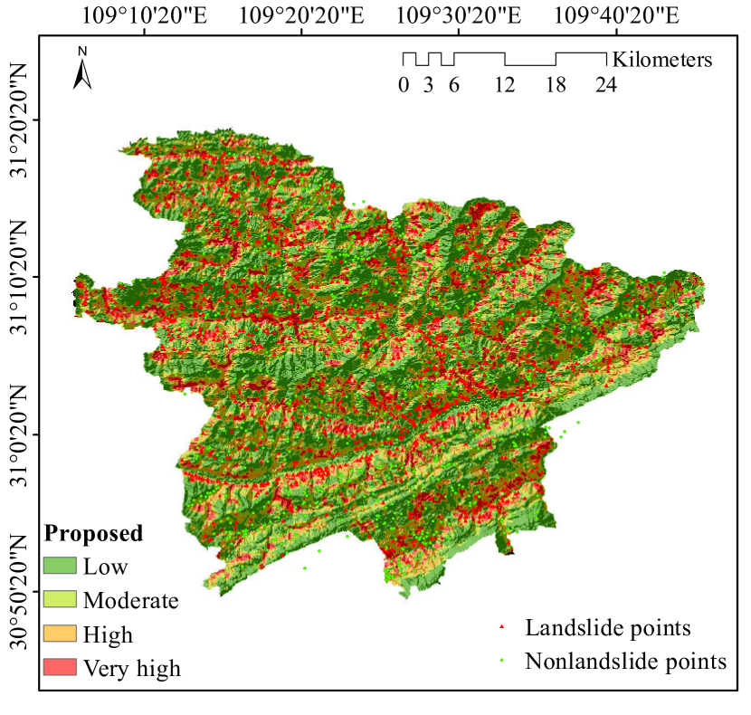
(e) proposed

Figure 7: LSM prediction in FJ with various methods.

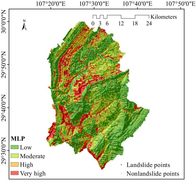
(a) MLP-based

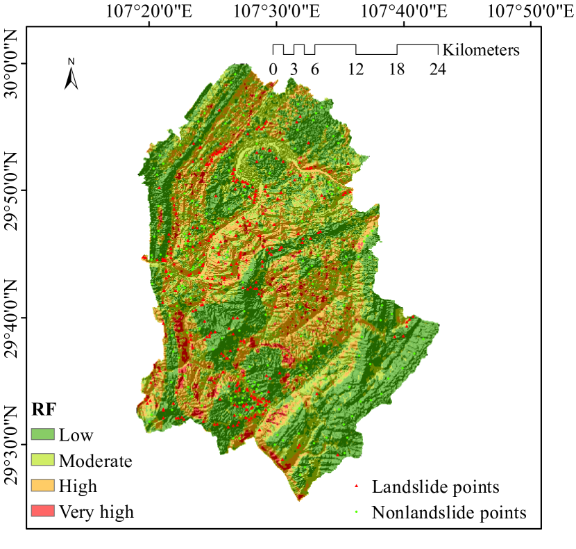
(b) RF-based

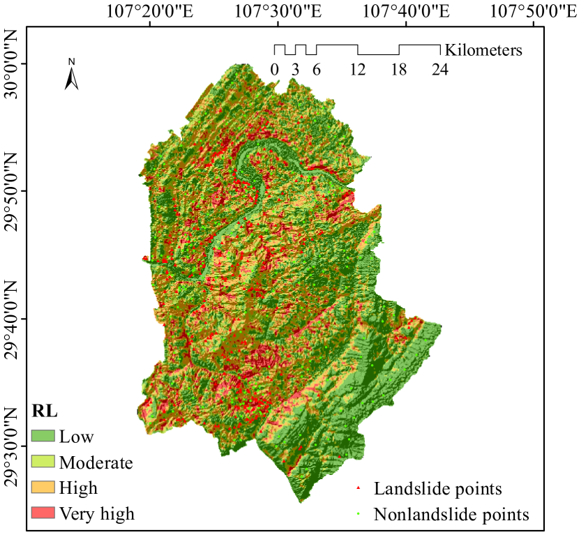
(c) RL-based

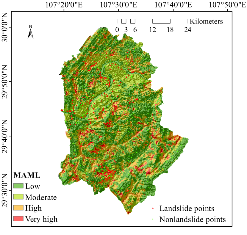
(d) MAML-based

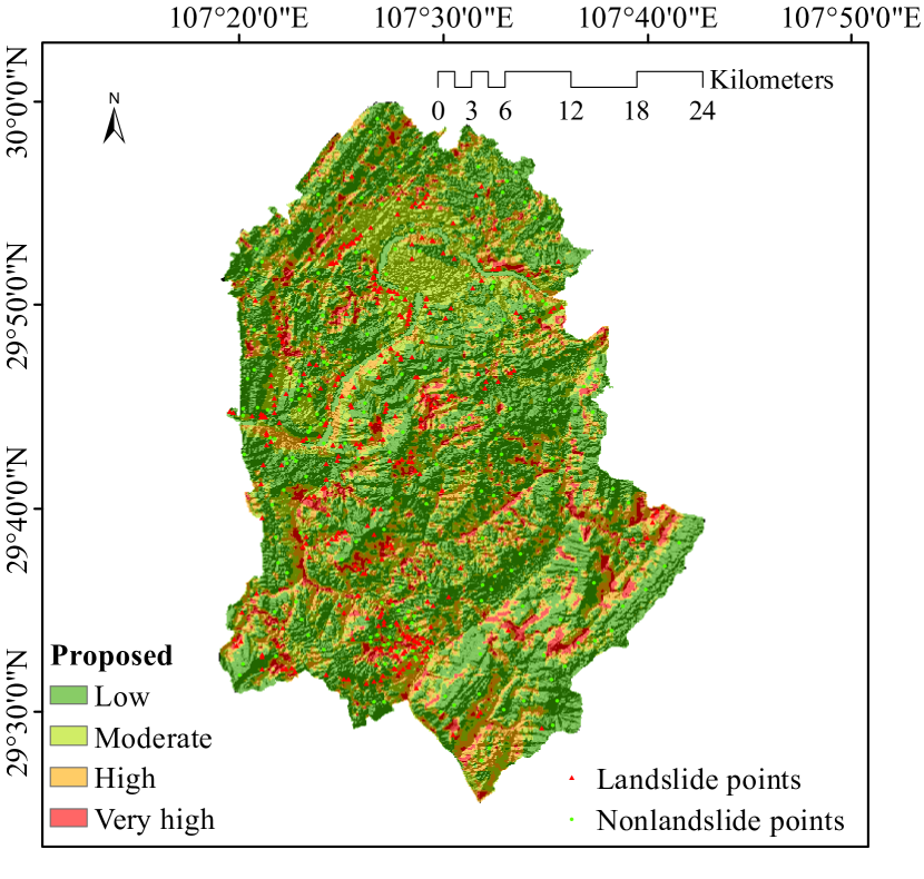
(e) proposed

Figure 8: LSM prediction in FL with various methods.

All methods predicted plausible LSMs in the FJ area with numerous evenly distributed samples, whereas in the sample-scarce area FL, the predictions were noticeably different. The MLP-based method showed a preference for positive prediction to the west of FL, where landslide samples were concentrated, while negative prediction was shown to the east of FL, where landslide samples were scarce, indicating that the predictive model was trapped in the local minimum. The LSM predicted by RF tended to produce discontinuous patches, reflecting from the side that the model suffered from overfitting. Zhu et al. (2020a) gives a more evident and interpretable result, in that some dominant causative factors, for example, distance to the drainage, slope, and strata type, should exert more significant influence on predicting the LSM. However, that method was also vulnerable to having very few samples because it failed to capture prominent conceptions in the east FL quickly. Additionally, the model lost sight of the discrepancy between landslide-inducing environments in different parts of the FL. In comparison, our method learns a general intermediate model such that vital conception can be quickly learned for local tasks with fewer samples and iterations.

For the intuitionistic perception of the landslide susceptibility prediction results, the LSMs of some parts of the FJ and FL regions are displayed in Fig. 9 and Fig. 10. The distance to the river and road has played an important role in landslides, whereas the residential areas are normally assigned with low landslide susceptibility. The proposed model has likely captured certain vital aspects in the few-shot adaption process. In addition, the figures also highlight indeed occurred landslides with high susceptibility, which proves the validity and reasonability of our method.

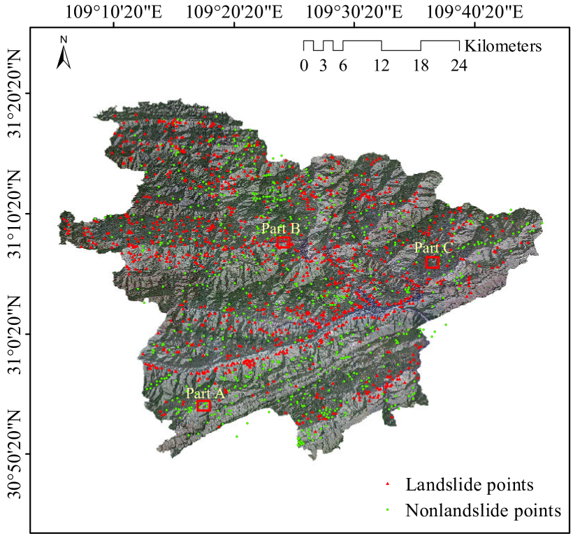
(a) FJ area

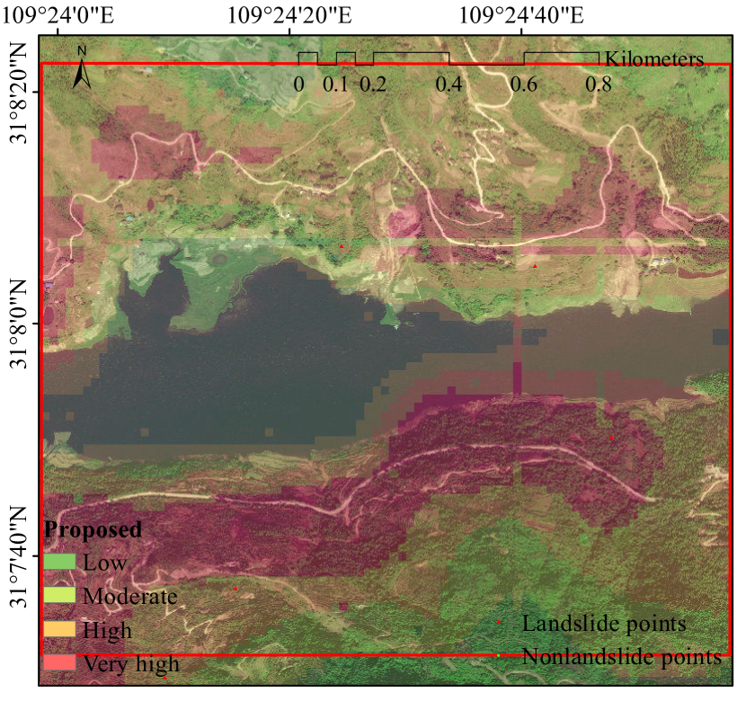
(b) LSM of Part A

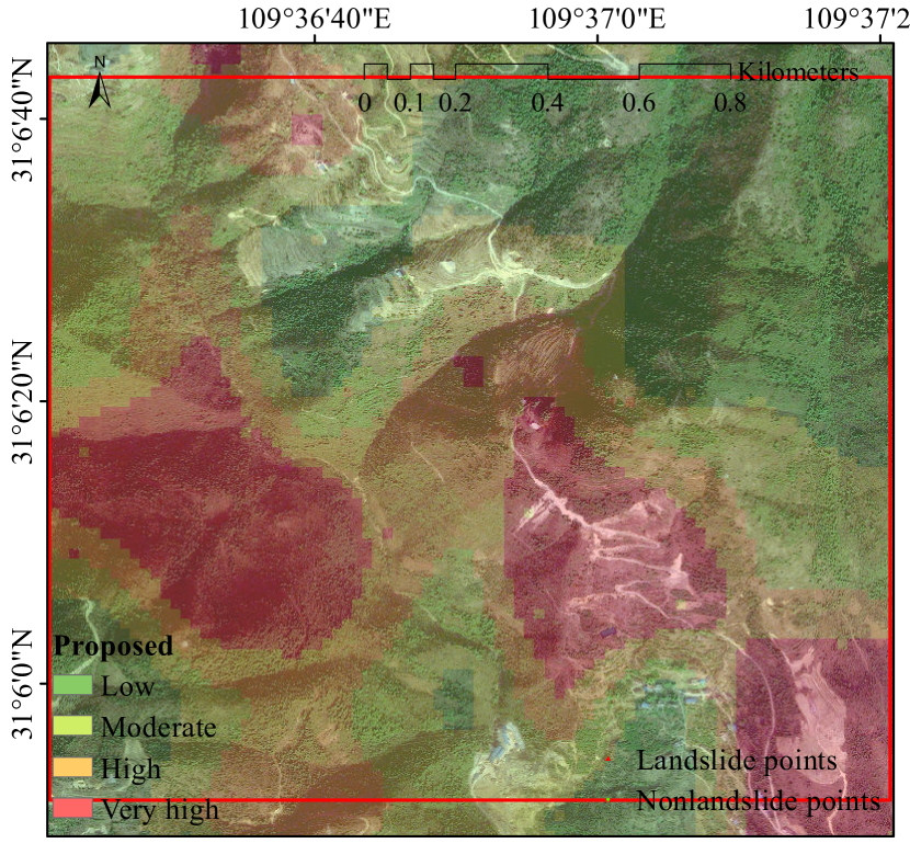
(c) LSM of Part B

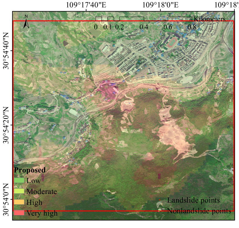
(d) LSM of Part C

Figure 9: Display of LSMs in various parts of FJ. Specifically, we chose three typical landforms: water (part A), mountainous (part B), and residential areas (part C).

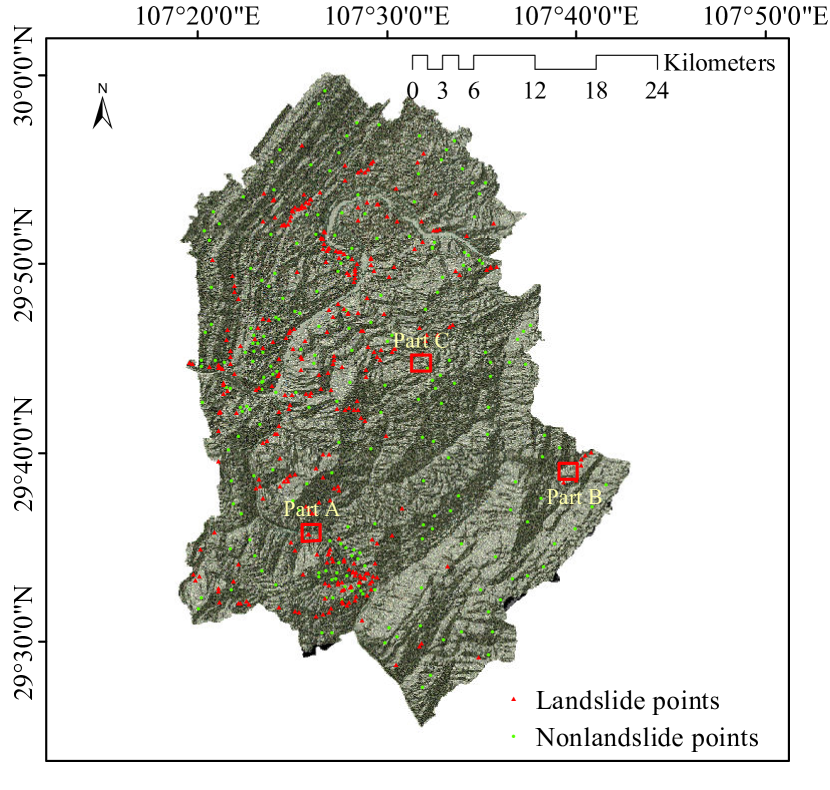
(a) FJ area

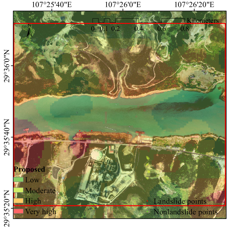
(b) LSM of Part A

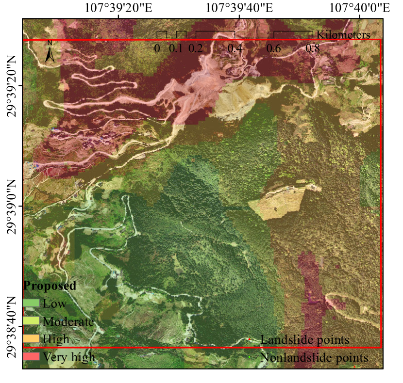
(c) LSM of Part B

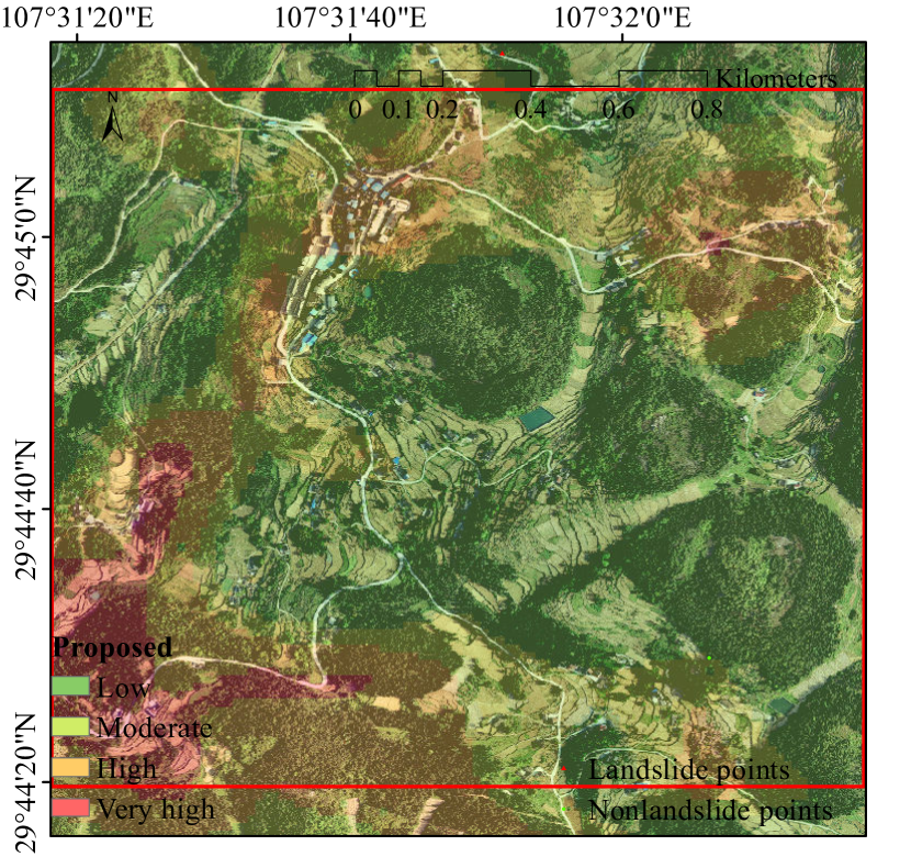
(d) LSM of Part C

Figure 10: Display of LSMs in various parts of FL. Specifically, we chose three typical landforms: water (part A), mountainous (part B), and residential areas (part C).

5.1.2 Performance evaluation

In this section, we bring in (Merghadi et al., 2018) some statistical measures to prove the validity of our method, which includes accuracy, precision, recall, and F1-score. They are given in Eq. 7,

$$\begin{split}\begin{aligned} Accuracy&=\frac{TP+TN}{TP+FP+TN+FN},\\ Precision&=\frac{TP}{TP+FP},\\ Recall&=\frac{TP}{TP+FN},\\ F1-score&=\frac{2TP}{2TP+FP+FN},\end{aligned}\end{split}$$ (7)

where $TN$, $TP$, $FN$, and $FP$ denote the Ture negative, true positive, false negative, and false positive, respectively.

Table 1: Performance comparison of various LSM models in FJ and FL. Despite the difficulties to few-shot learn the predictive models, our method still reaches the state-of-the-art.

Study areas	Models	Accuracy(%)	Precision(%)	Recall(%)	F1-score(%)
FJ	MLP	73.5	72.3	69.9	70.9
	RF	74.8	74.7	65.3	69.4
	RL	74.9	70.2	77.5	77.3
	MAML	72.6	69.3	72.7	68.3
	Proposed	75.1	72.0	76.6	74.0
FL	MLP	76.7	77.1	76.6	76.6
	RF	77.8	80.1	73.3	76.3
	RL	81.6	78.7	85.6	81.2
	MAML	76.4	83.7	83.4	82.0
	Proposed	78.4	86.9	83.5	85.0

Table 1 shows the performance of various methods in FJ and FL. The proposed method provides the highest accuracy of 75.1% in FJ. Also, it performs pretty well on other statistical measures, even with a few samples and gradient updates for adaption. It is different from MLP-based (Zare et al., 2013), RF-based (Catani et al., 2013), and RL-based (Zhu et al., 2020a) methods trained by whole samples within a ministrative region with hundreds or thousands of update iterations. It verifies the feasibility of assuming that various parts of a ministrative region could possess different landslide causes, and the LSM predictive model of each block could be few-shot learned. In addition, compared to the typical few-shot learning approach MAML (Finn et al., 2017), the adopted tricks realize distinct improvements in performance.

5.2 Effect of unsupervised pretraining

To explore the properties of unsupervised learned representation, we utilized some visualization approaches, including principal component analysis (PCA) (Wold et al., 1987), Isomap (Balasubramanian et al., 2002), t-distributed stochastic neighbor embedding (t-SNE) (Van der Maaten and Hinton, 2008), and uniform manifold approximation and projection (UMAP) (McInnes et al., 2018), to visualize the embedding spaces of the original data, the MAML-based method without an unsupervised training process, and the proposed method, as shown in Table 2. The left column shows the embedding results inferred from the original input space. The middle column shows the embedding results inferred from representations learned by the MAML-based method. The right column shows the embedding results inferred from the proposed learned representation. The red and blue points respectively denote landslide and non-landslide samples.

Table 2: Three-dimensional visualization of embedding space when given only 5 samples ($K=5$) for adaption in FJ.

Embedding	Original data	Without pretraining	Proposed
PCA
Isomap
t-SNE
UMAP

Table 3: The ablation experiment where we meta-train part of FJ and FL, and test the other part of FJ and FL. ($M$ is the number of samples within a task)

Ablation experiment	Backbone	Number of labelled samples
		$K=1$	$K=5$	$K=M/2$
Without unsupervised pretraining	MAML-based	67.1$\pm$4.5	68.8$\pm$4.2	72.3$\pm$3.4
	proposed	67.4$\pm$3.6	72.1$\pm$3.1	75.5$\pm$3.3
With unsupervised pretraining	MAML-based	69.0$\pm$3.7	70.9$\pm$3.1	73.7$\pm$2.9
	proposed	69.5$\pm$2.8	73.4$\pm$2.4	76.9$\pm$2.1

The essence of these visualization approaches is to explore a discriminative embedding space, wherein the consecutiveness or aggregation of points of the same kind can reflect the performance of the visualization approach (Becht et al., 2019). Certainly, the unsupervised training process finds a representation that is easier to be embedded in a discriminative space that is suited for supervision tasks. In addition, we present the measurement performance of the ablation experiment, as shown in Table 3. The overall performance improvements proved the validity of the unsupervised pretraining process.

5.3 Analysis of the meta-learner

5.3.1 Weakening the adverse effect of inaccurate supervision

One crucial problem this study aims to deal with is inaccurate supervision, in which labeled samples do not always reflect the ground truth (Zhang et al., 2021). It occurs because landslide samples are collected from historical records and potential inferred landslides. The occurrence of historical landslides is a certain contingency, and experts infer potential landslides according to prior knowledge, both of which would lead to certain inaccuracies in the marking of landslide samples. That is different from a picture sample from which precise contents and objects can be confirmed, or samples can be identified with definite labeling meanings. Given this, the proposed meta-learner designed a trick to weigh the task losses to alleviate the adverse effects of inaccurate supervision, as discussed in Section 4.4. To compare the performance in terms of stability and overall accuracy (OA), we (meta) train part of the samples of FJ and FL and then test the other part of the samples of FJ and FL. The performance can be seen in Fig. 11.

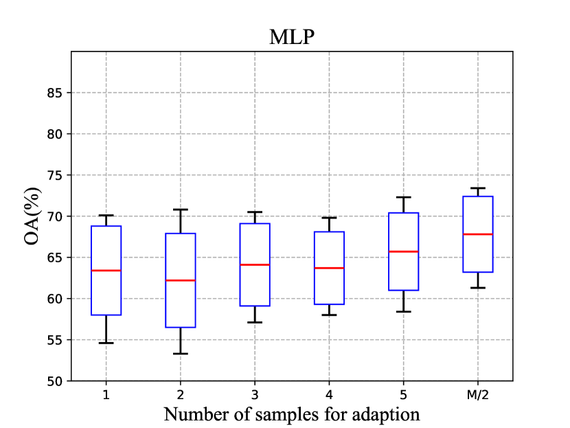
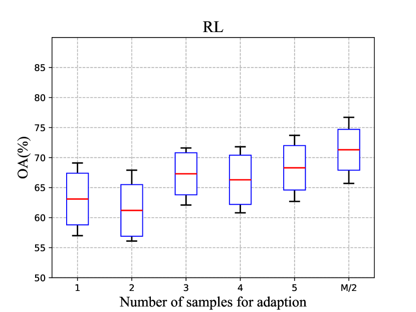
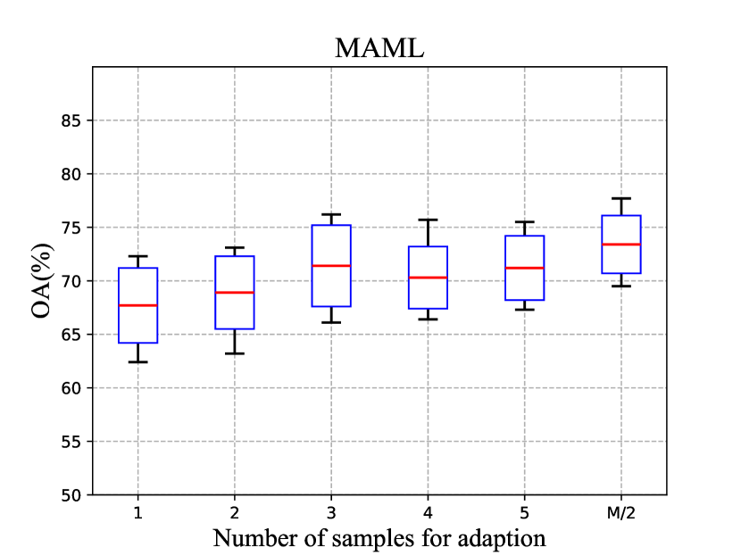
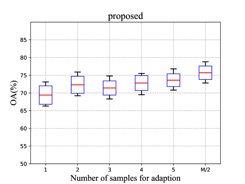
Figure 11: The candle charts for evaluating the overall performance of different methods. The red line represents the mean OA, which lies in the middle of the bar. The height of the bar indicates two times the standard deviation. The horizontal black line indicates the maximum OA and minimum OA.

The OA of the MLP-based method did not improve significantly as the number of samples increased, illustrating the limitation of learning with only a few samples. The RL-based method slightly improves but is unstable with a high standard deviation. The MAML-based method increases the OA to a new height but also suffers from instability owing to the adverse effect of inaccurate supervision. Instead, the proposed method realizes the best OA and stability. Because of the correlation of input features, direct feeding of the original data to the supervision task would mislead the learner to weigh the contribution of the features wrongly. It can reflect the embedding space of the MAML-based method that not a few positive and negative samples are still confusedly mixed in some dimensions.

5.3.2 Few-shot learning performance and generalization ability comparison

To comprehensively explore the few-shot learning performance and generalization ability comparison of various methods, we designed four groups of comparative experiments, as shown in Tables 4, 5, 6, and 7, where $K$ denotes the number of samples used for adaptation, and $M$ ($M>5$) denotes the number of samples within a task. The methods that participated in the comparison were classified as transferring-based and meta-learning-based for their adaption. The four experiments were: A. (meta) training part samples of FJ, and then testing the other part samples of FJ; B. (meta) training all samples of FJ, and then testing all samples of FL; C. (meta) training part samples of FJ and part samples of FL, then testing the other part samples of FJ; D. (meta) training all samples of FJ and part samples of FL, then testing the other part samples of FL. The number of gradient descent updates for adaption in all experiments was set to 5. Fig. 16 gives the receiver operating characteristic (ROC) curves of these methods in each experiment, where class 1 and class 2 represent the non-landslide and landslide classes, respectively. Also, Fig. 12 present the OA performance with a different number of labeled samples.

Table 4: Overall accuracy (OA) of various methods in experiment A: (meta) training part samples of FJ, and then testing the other part of FJ.

Experiment	Categories	Backbone	Number of labelled samples
			$K=1$	$K=5$	$K=M/2$
A	Transferring-based	MLP-based	62.2$\pm$4.8	64.5$\pm$4.9	65.6$\pm$4.2
		RL-based	66.9$\pm$4.3	68.2$\pm$3.5	70.2$\pm$3.1
	Meta-learning-based	MAML-based	67.9$\pm$3.4	69.9$\pm$2.3	70.7$\pm$1.7
		Proposed	68.3$\pm$2.4	72.2$\pm$1.6	74.7$\pm$0.7

Table 5: Overall accuracy (OA) of various methods in experiment B: (meta) training all samples of FJ, then testing all samples of FL.

Experiment	Categories	Backbone	Number of labelled samples
			$K=1$	$K=5$	$K=M/2$
B	Transferring-based	MLP-based	64.2$\pm$6.2	66.5$\pm$5.4	67.9$\pm$4.1
		RL-based	70.1$\pm$4.6	69.8$\pm$4.7	70.5$\pm$3.2
	Meta-learning-based	MAML-based	69.9$\pm$3.2	70.7$\pm$2.9	72.4$\pm$2.6
		Proposed	71.3$\pm$2.5	72.7$\pm$2.3	75.1$\pm$1.9

Table 6: Overall accuracy (OA) of various methods in experiment C: (meta) training part samples of FJ and part samples of FL, then testing the other part of FJ.

Experiment	Categories	Backbone	Number of labelled samples
			$K=1$	$K=5$	$K=M/2$
C	Transferring-based	MLP-based	63.2$\pm$5.5	63.9$\pm$5.9	65.4$\pm$4.5
		RL-based	63.7$\pm$4.9	66.7$\pm$3.1	69.5$\pm$3.2
	Meta-learning-based	MAML-based	67.1$\pm$3.2	68.9$\pm$2.7	72.6$\pm$2.4
		Proposed	67.5$\pm$2.0	71.5$\pm$1.4	75.3$\pm$1.7

Table 7: Overall accuracy (OA) of various methods in experiment D: (meta) training all samples of FJ and part samples of FL, then testing the other part FL.

Experiment	Categories	Backbone	Number of labelled samples
			$K=1$	$K=5$	$K=M/2$
D	Transferring-based	MLP-based	64.5$\pm$6.2	70.4$\pm$6.1	72.8$\pm$5.4
		RL-based	65.8$\pm$5.6	71.9$\pm$4.1	74.3$\pm$4.6
	Meta-learning-based	MAML-based	72.1$\pm$4.2	73.2$\pm$3.8	76.4$\pm$3.5
		Proposed	72.8$\pm$3.0	75.3$\pm$2.6	78.4$\pm$2.5

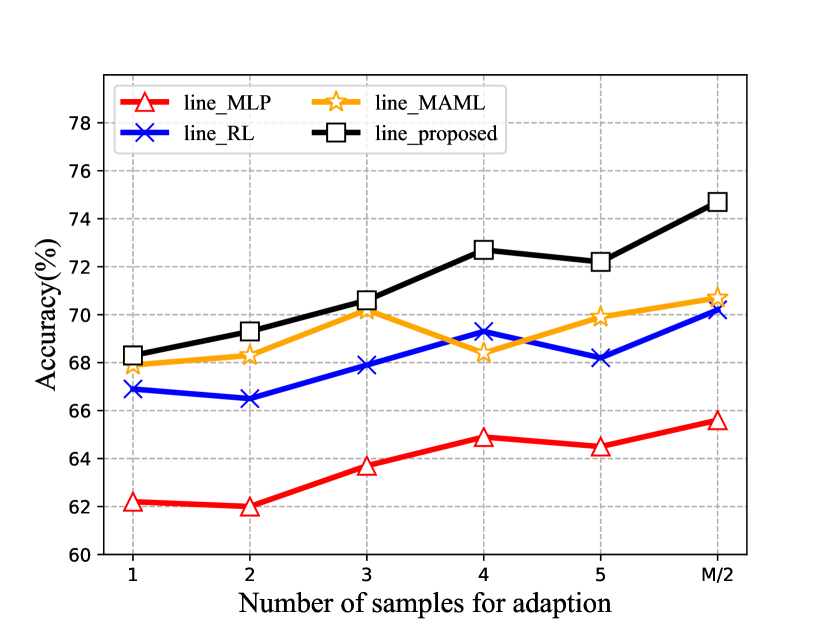
(a) Experiment A

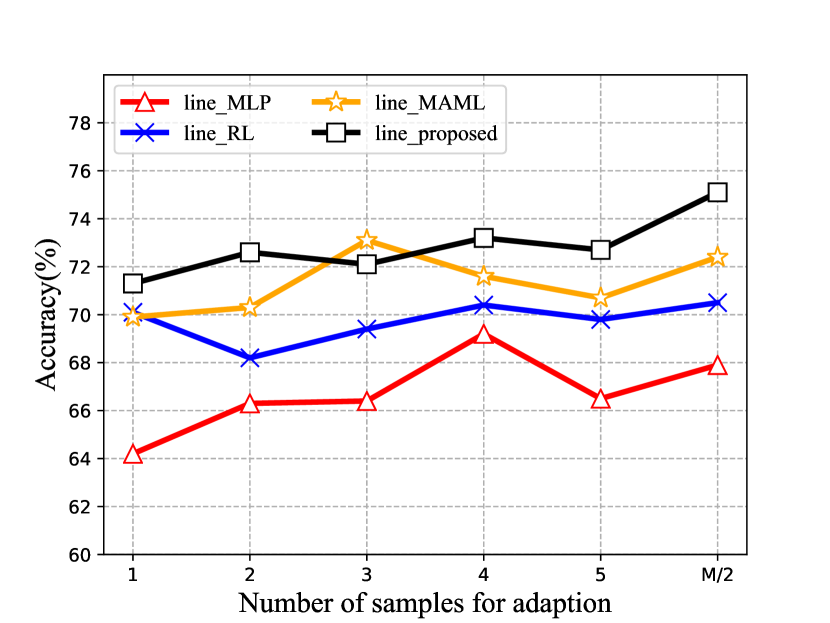
(b) Experiment B

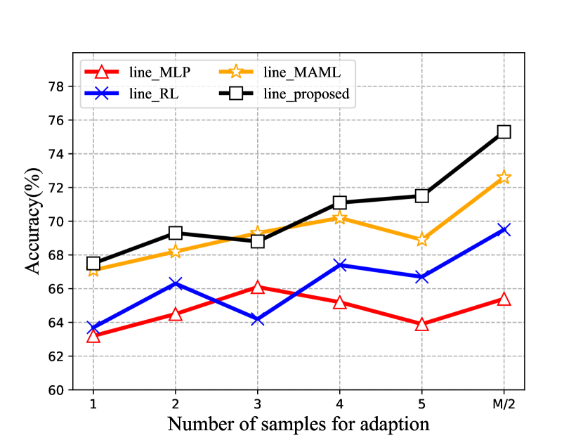
(c) Experiment C

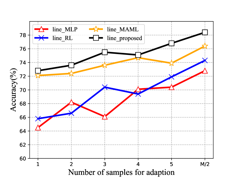
(d) Experiment D

Figure 12: OA performance with different numbers of labeled samples.

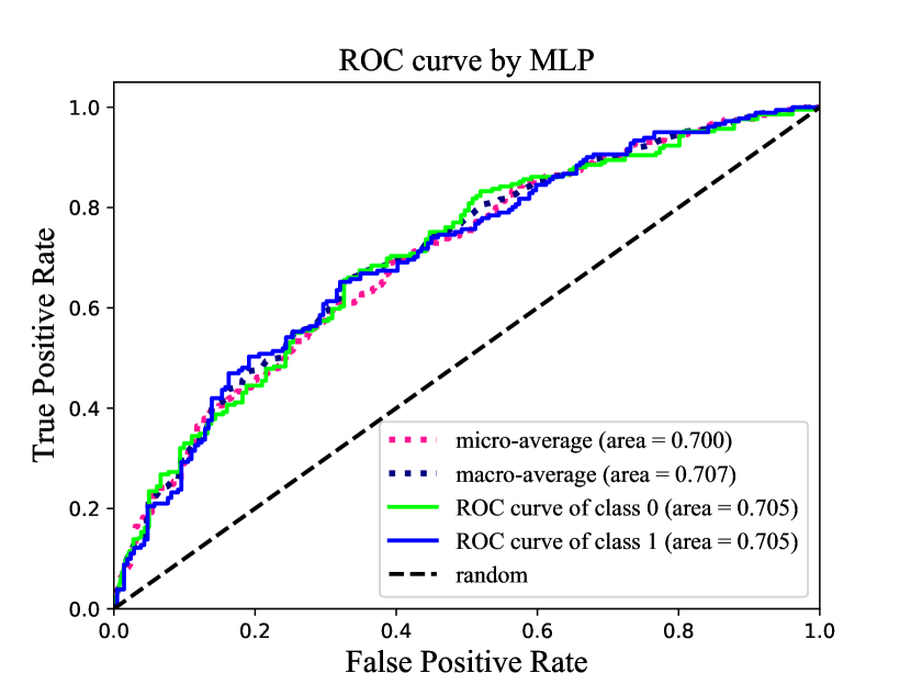
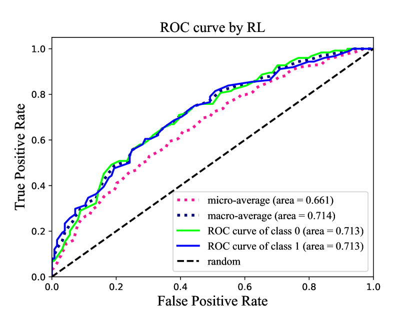
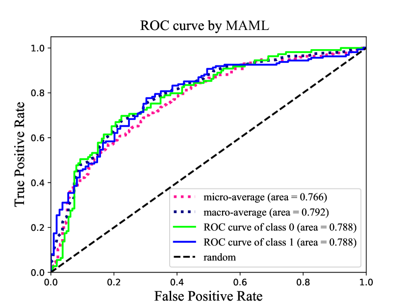
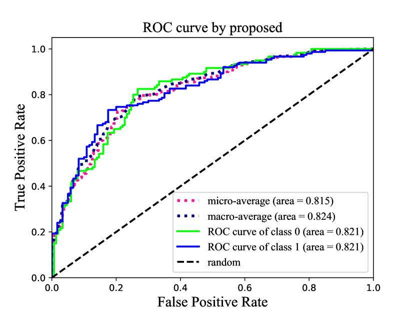
Figure 13: ROC curves of Experiment A.

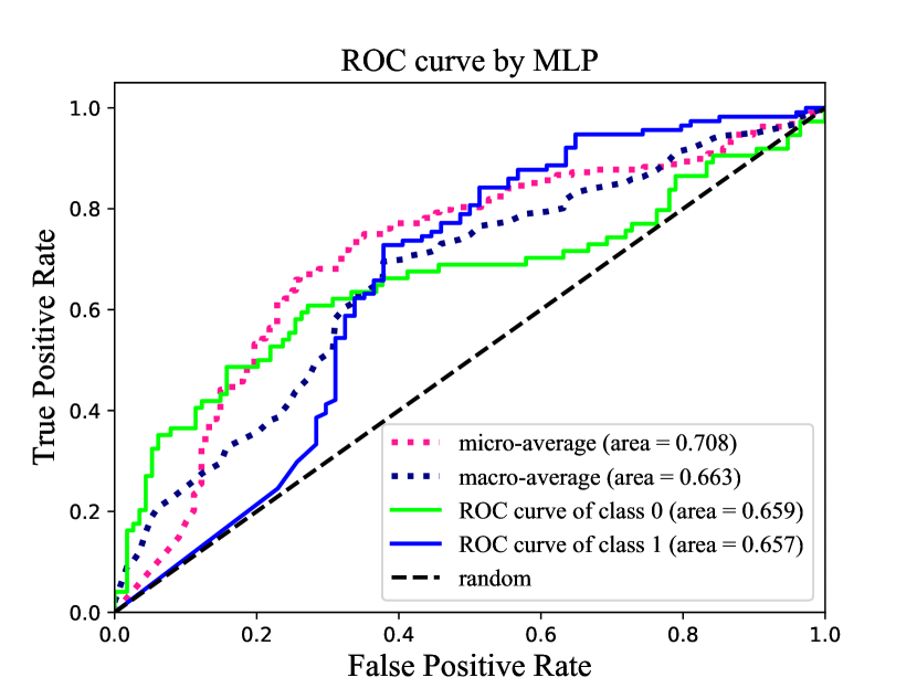
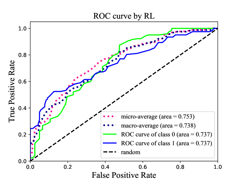
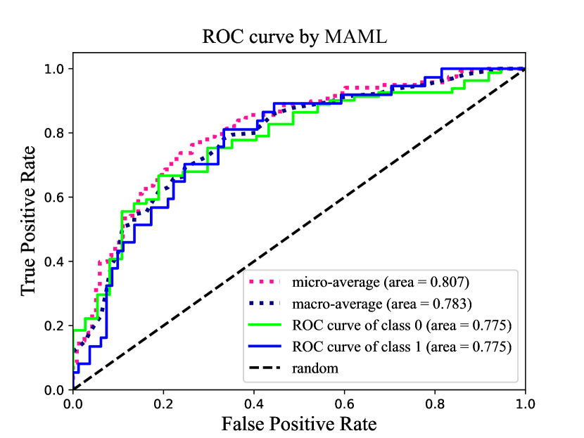
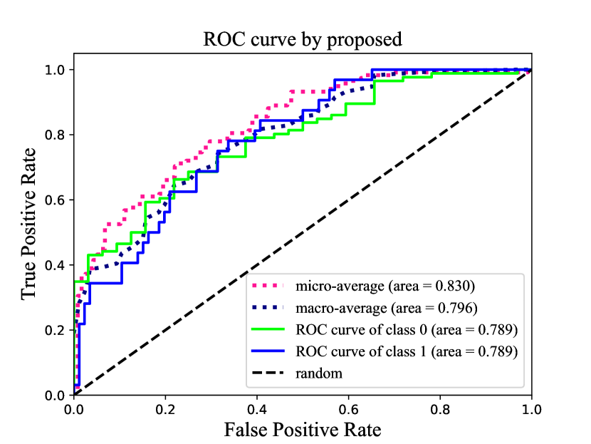
Figure 14: ROC curves of Experiment B.

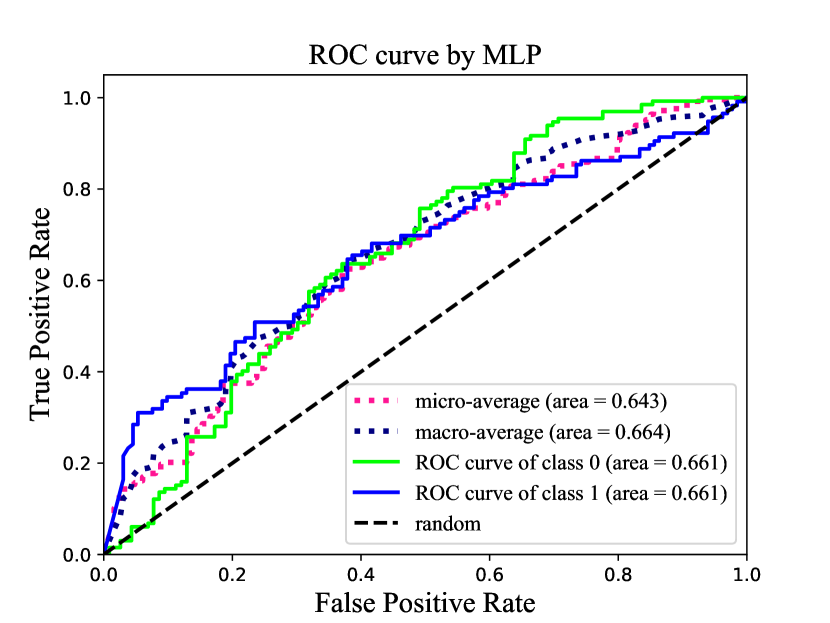
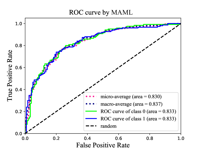
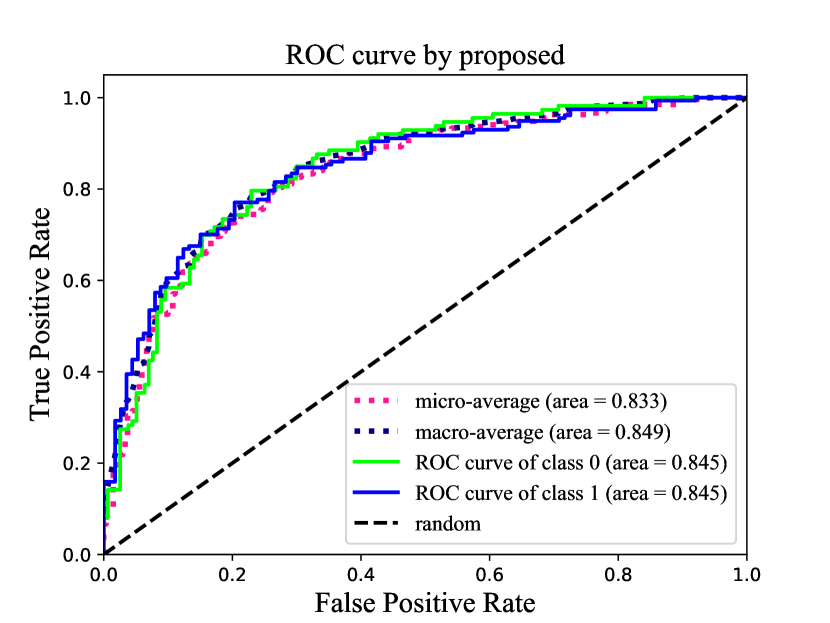
Figure 15: ROC curves of Experiment C.

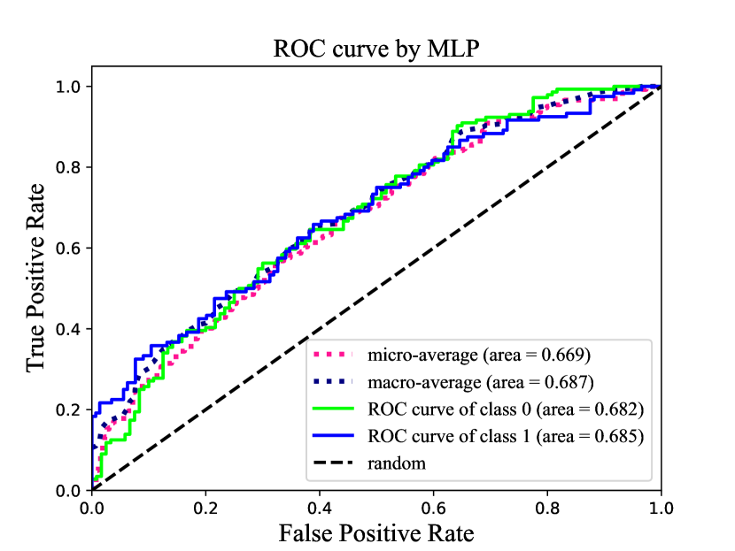
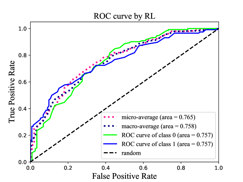
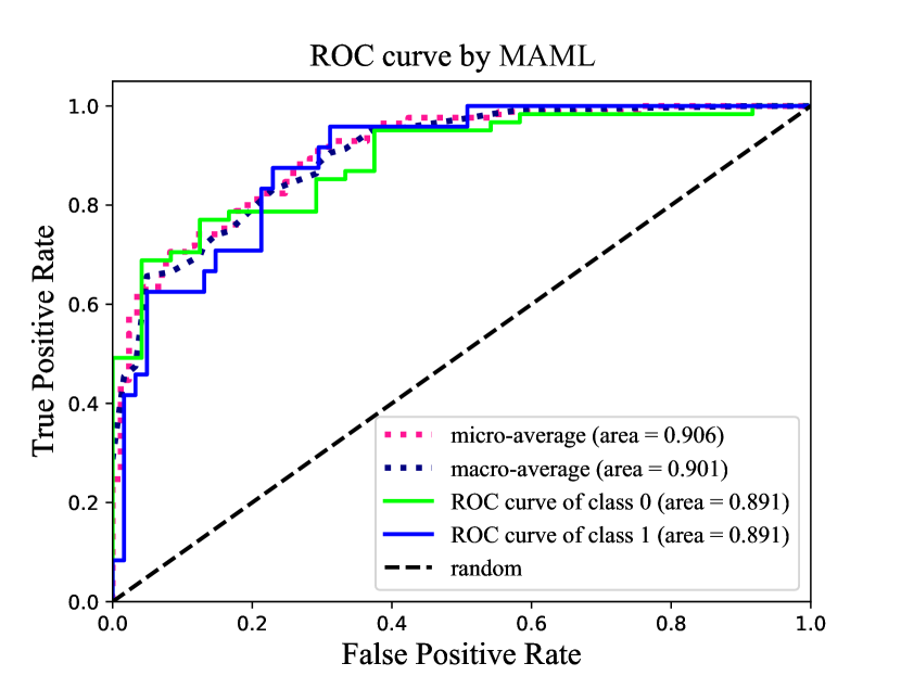
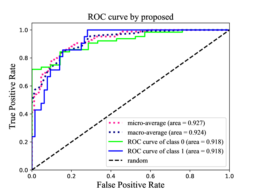
Figure 16: ROC curves of Experiment D.

From all the experiments, we find that the meta-learning-based methods evidently improve their performance with an increase in $K$, whereas the transferring-based methods improve relatively little. That demonstrates the validity of applying the meta-learning ideology to realize fast adaption with very few samples and iterations in the LSM territory. In addition, with our proposed tricks, we further improve the performance to the top level.

In experiments A and B, where there are plenty of samples in FJ, the few-shot learning performance of the proposed method is better than the others. From experiment B, we find that the generalization ability of the proposed methods from FJ to FL also outperforms the others. It is worth noting that the accuracy in Zhu et al. (2020a) is close to meta-learning-based methods when $K=1$ because the applied adversarial training has learned shared factors that can be directly transferred between FJ and FL scenarios (Goodfellow et al., 2014).

From the comparison with experiment A and C, we can see that meta-training together with FJ and FL tasks improves the overall performance of meta-learning-based methods. In this study, we attribute this to the fact that productive tasks containing various landslide-inducing environments contribute to a more general intermediate model, that is, improving the generalization ability of the intermediate model. This claim can also be confirmed from a comparison with experiments B and D. Thus, experiment C was used to predict the LSM of FJ, while experiment D was used to predict the LSM of FL.

6 Conclusion

In response to the two problems mentioned in Section 1.1 and 1.2, our proposed method meta-learns an intermediate representation for the few-shot prediction of landslide susceptibility. The experiment and results demonstrate the validity of (1) applying unsupervised pretraining to discover discriminative embedding space; (2) segmenting large scenarios into pieces for individual analysis; and (3) meta-learning an intermediate representation for fast adaptation to new local tasks.

This study presents the first example of a block-wise prediction of landslide susceptibility in a meta-learning manner to the best of our knowledge. Considering the tiny amount of samples and gradient descent updates used when adapting to a new task, the proposed architecture outperforms in terms of stability to inaccurate supervision, generalization ability, and fast adaption performance. It proves the validity and superiority of applying our method to large scenarios where the landslide-inducing environment is various and complex, and landslide samples are very few. We also summarize the limitations of our proposed method as follows.

(1) Samples in meta-training were limited in FJ and FL, thus if possible, samples from other areas, accounting for different landslide causes, could be added into the meta-learner to improve the generalization ability and fast adaption ability of the intermediate model.

(2) Because many of the parameter settings, for example, the update learning rate, number of meta tasks, and number of adapting updates, are not determined automatically, but experimentally, it becomes necessary to validate the appropriate value by repeating the running of the code.

(3) The unbalanced distribution of positive and negative samples would cause an adverse tendency to predict LSM. For example, if one block is only full of positive samples, the adapted model will tend to give a positive prediction of that block. It is demonstrated in Fig. 8. Nevertheless, the proposed method still performs better than the other methods.

CRediT author statement

Li Chen: Conceptualization, Methodology, Software, Investigation, Writing - Original Draft, Data Curation. Yulin Ding: Supervision, Project administration, Funding acquisition. Saeid Pirasteh: Formal analysis, Writing - Review & Editing. Han Hu: Methodology, Writing - Review & Editing, Funding acquisition. Qing Zhu: Project administration, Funding acquisition. Xuming Ge: Resources. Haowei Zeng: Validation. Haojia Yu: Formal analysis. Qisen Shang: Formal analysis. Yongfei Song: Funding acquisition.

Declaration of Competing Interest

The authors declare that they have no known competing financial interests or personal relationships that could have appeared to influence the work reported in this paper.

References

- Achanta et al. (2012) Achanta, R., Shaji, A., Smith, K., Lucchi, A., Fua, P., Süsstrunk, S., 2012. Slic superpixels compared to state-of-the-art superpixel methods. IEEE transactions on pattern analysis and machine intelligence 34, 2274–2282.
- Amruthnath and Gupta (2018) Amruthnath, N., Gupta, T., 2018. A research study on unsupervised machine learning algorithms for early fault detection in predictive maintenance, in: 2018 5th International Conference on Industrial Engineering and Applications (ICIEA), IEEE. pp. 355–361.
- Balasubramanian et al. (2002) Balasubramanian, M., Schwartz, E.L., Tenenbaum, J.B., de Silva, V., Langford, J.C., 2002. The isomap algorithm and topological stability. Science 295, 7–7.
- Becht et al. (2019) Becht, E., McInnes, L., Healy, J., Dutertre, C.A., Kwok, I.W., Ng, L.G., Ginhoux, F., Newell, E.W., 2019. Dimensionality reduction for visualizing single-cell data using umap. Nature biotechnology 37, 38–44.
- Catani et al. (2013) Catani, F., Lagomarsino, D., Segoni, S., Tofani, V., 2013. Landslide susceptibility estimation by random forests technique: sensitivity and scaling issues. Natural Hazards and Earth System Sciences 13, 2815–2831.
- Chang et al. (2020) Chang, Z., Du, Z., Zhang, F., Huang, F., Chen, J., Li, W., Guo, Z., 2020. Landslide susceptibility prediction based on remote sensing images and gis: Comparisons of supervised and unsupervised machine learning models. Remote Sensing 12, 502.
- Chen et al. (2018) Chen, W., Shahabi, H., Zhang, S., Khosravi, K., Shirzadi, A., Chapi, K., Pham, B.T., Zhang, T., Zhang, L., Chai, H., et al., 2018. Landslide susceptibility modeling based on gis and novel bagging-based kernel logistic regression. Applied Sciences 8, 2540.
- Chen et al. (2019) Chen, Z., Liang, S., Ke, Y., Yang, Z., Zhao, H., 2019. Landslide susceptibility assessment using evidential belief function, certainty factor and frequency ratio model at baxie river basin, nw china. Geocarto International 34, 348–367.
- Ciampalini et al. (2016) Ciampalini, A., Raspini, F., Lagomarsino, D., Catani, F., Casagli, N., 2016. Landslide susceptibility map refinement using psinsar data. Remote Sensing of Environment 184, 302–315.
- CNIC (2021) CNIC, C., 2021. Geospatial data cloud. http://www.gscloud.cn/.
- Dou et al. (2019) Dou, J., Yunus, A.P., Bui, D.T., Merghadi, A., Sahana, M., Zhu, Z., Chen, C.W., Khosravi, K., Yang, Y., Pham, B.T., 2019. Assessment of advanced random forest and decision tree algorithms for modeling rainfall-induced landslide susceptibility in the izu-oshima volcanic island, japan. Science of the total environment 662, 332–346.
- Fan et al. (2018) Fan, X., Zhan, W., Dong, X., van Westen, C., Xu, Q., Dai, L., Yang, Q., Huang, R., Havenith, H.B., 2018. Analyzing successive landslide dam formation by different triggering mechanisms: The case of the tangjiawan landslide, sichuan, china. Engineering geology 243, 128–144.
- Fang et al. (2020) Fang, Z., Wang, Y., Peng, L., Hong, H., 2020. Integration of convolutional neural network and conventional machine learning classifiers for landslide susceptibility mapping. Computers & Geosciences 139, 104470.
- Finn et al. (2017) Finn, C., Abbeel, P., Levine, S., 2017. Model-agnostic meta-learning for fast adaptation of deep networks, in: International Conference on Machine Learning, PMLR. pp. 1126–1135.
- Ge and Zhu (2021) Ge, X., Zhu, Q., 2021. Target-based automated matching of multiple terrestrial laser scans for complex forest scenes. ISPRS Journal of Photogrammetry and Remote Sensing 179, 1–13.
- Goldblum et al. (2020) Goldblum, M., Reich, S., Fowl, L., Ni, R., Cherepanova, V., Goldstein, T., 2020. Unraveling meta-learning: Understanding feature representations for few-shot tasks, in: International Conference on Machine Learning, PMLR. pp. 3607–3616.
- Goodfellow et al. (2014) Goodfellow, I.J., Pouget-Abadie, J., Mirza, M., Xu, B., Warde-Farley, D., Ozair, S., Courville, A., Bengio, Y., 2014. Generative adversarial networks. arXiv preprint arXiv:1406.2661 .
- Hinton (2002) Hinton, G.E., 2002. Training products of experts by minimizing contrastive divergence. Neural computation 14, 1771–1800.
- Hinton (2007) Hinton, G.E., 2007. Boltzmann machine. Scholarpedia 2, 1668.
- Hoffmann et al. (2011) Hoffmann, R., Zhang, C., Ling, X., Zettlemoyer, L., Weld, D.S., 2011. Knowledge-based weak supervision for information extraction of overlapping relations, in: Proceedings of the 49th annual meeting of the association for computational linguistics: human language technologies, pp. 541–550.
- Hong et al. (2020) Hong, H., Liu, J., Zhu, A.X., 2020. Modeling landslide susceptibility using logitboost alternating decision trees and forest by penalizing attributes with the bagging ensemble. Science of the total environment 718, 137231.
- Hospedales et al. (2020) Hospedales, T., Antoniou, A., Micaelli, P., Storkey, A., 2020. Meta-learning in neural networks: A survey. arXiv preprint arXiv:2004.05439 .
- Hu et al. (2021) Hu, X., Mei, H., Zhang, H., Li, Y., Li, M., 2021. Performance evaluation of ensemble learning techniques for landslide susceptibility mapping at the jinping county, southwest china. Natural Hazards 105, 1663–1689.
- Huang and Zhao (2018) Huang, Y., Zhao, L., 2018. Review on landslide susceptibility mapping using support vector machines. Catena 165, 520–529.
- Jebur et al. (2014) Jebur, M.N., Pradhan, B., Tehrany, M.S., 2014. Optimization of landslide conditioning factors using very high-resolution airborne laser scanning (lidar) data at catchment scale. Remote Sensing of Environment 152, 150–165.
- Lin et al. (2013) Lin, M., Chen, Q., Yan, S., 2013. Network in network. arXiv preprint arXiv:1312.4400 .
- Van der Maaten and Hinton (2008) Van der Maaten, L., Hinton, G., 2008. Visualizing data using t-sne. Journal of machine learning research 9.
- McInnes et al. (2018) McInnes, L., Healy, J., Melville, J., 2018. Umap: Uniform manifold approximation and projection for dimension reduction. arXiv preprint arXiv:1802.03426 .
- Merghadi et al. (2018) Merghadi, A., Abderrahmane, B., Tien Bui, D., 2018. Landslide susceptibility assessment at mila basin (algeria): a comparative assessment of prediction capability of advanced machine learning methods. ISPRS International Journal of Geo-Information 7, 268.
- Merghadi et al. (2020) Merghadi, A., Yunus, A.P., Dou, J., Whiteley, J., ThaiPham, B., Bui, D.T., Avtar, R., Abderrahmane, B., 2020. Machine learning methods for landslide susceptibility studies: A comparative overview of algorithm performance. Earth-Science Reviews , 103225.
- Metz et al. (2018) Metz, L., Maheswaranathan, N., Cheung, B., Sohl-Dickstein, J., 2018. Meta-learning update rules for unsupervised representation learning. arXiv preprint arXiv:1804.00222 .
- Nair and Hinton (2010) Nair, V., Hinton, G.E., 2010. Rectified linear units improve restricted boltzmann machines, in: Icml.
- Pham et al. (2017) Pham, B.T., Bui, D.T., Prakash, I., Dholakia, M., 2017. Hybrid integration of multilayer perceptron neural networks and machine learning ensembles for landslide susceptibility assessment at himalayan area (india) using gis. Catena 149, 52–63.
- Pham et al. (2019a) Pham, B.T., Jaafari, A., Prakash, I., Bui, D.T., 2019a. A novel hybrid intelligent model of support vector machines and the multiboost ensemble for landslide susceptibility modeling. Bulletin of Engineering Geology and the Environment 78, 2865–2886.
- Pham et al. (2019b) Pham, B.T., Prakash, I., Singh, S.K., Shirzadi, A., Shahabi, H., Bui, D.T., et al., 2019b. Landslide susceptibility modeling using reduced error pruning trees and different ensemble techniques: Hybrid machine learning approaches. Catena 175, 203–218.
- Popescu (2002) Popescu, M.E., 2002. Landslide causal factors and landslide remediatial options, in: 3rd International Conference on Landslides, Slope Stability and Safety of Infra-Structures, Citeseer. pp. 61–81.
- Qing et al. (2019) Qing, Z., Haowei, Z., Yulin, D., Xiao, X., Fei, L., Liguo, Z., Haifeng, L., Han, H., Junxiao, Z., Li, C., et al., 2019. A review of major potential landslide hazards analysis. Acta Geodaetica et Cartographica Sinica 48, 1551.
- Ray et al. (2010) Ray, R.L., Jacobs, J.M., Cosh, M.H., 2010. Landslide susceptibility mapping using downscaled amsr-e soil moisture: A case study from cleveland corral, california, us. Remote sensing of environment 114, 2624–2636.
- Reichenbach et al. (2018) Reichenbach, P., Rossi, M., Malamud, B.D., Mihir, M., Guzzetti, F., 2018. A review of statistically-based landslide susceptibility models. Earth-Science Reviews 180, 60–91.
- Ren et al. (2018) Ren, M., Triantafillou, E., Ravi, S., Snell, J., Swersky, K., Tenenbaum, J.B., Larochelle, H., Zemel, R.S., 2018. Meta-learning for semi-supervised few-shot classification. arXiv preprint arXiv:1803.00676 .
- Salakhutdinov and Hinton (2009) Salakhutdinov, R., Hinton, G., 2009. Deep boltzmann machines, in: Artificial intelligence and statistics, PMLR. pp. 448–455.
- Sameen et al. (2020) Sameen, M.I., Sarkar, R., Pradhan, B., Drukpa, D., Alamri, A.M., Park, H.J., 2020. Landslide spatial modelling using unsupervised factor optimisation and regularised greedy forests. Computers & Geosciences 134, 104336.
- Scaringi et al. (2018) Scaringi, G., Fan, X., Xu, Q., Liu, C., Ouyang, C., Domènech, G., Yang, F., Dai, L., 2018. Some considerations on the use of numerical methods to simulate past landslides and possible new failures: the case of the recent xinmo landslide (sichuan, china). Landslides 15, 1359–1375.
- Shahri and Moud (2021) Shahri, A.A., Moud, F.M., 2021. Landslide susceptibility mapping using hybridized block modular intelligence model. Bulletin of engineering geology and the environment 80, 267–284.
- Shahri et al. (2019) Shahri, A.A., Spross, J., Johansson, F., Larsson, S., 2019. Landslide susceptibility hazard map in southwest sweden using artificial neural network. Catena 183, 104225.
- Sun et al. (2021) Sun, D., Xu, J., Wen, H., Wang, D., 2021. Assessment of landslide susceptibility mapping based on bayesian hyperparameter optimization: A comparison between logistic regression and random forest. Engineering Geology 281, 105972.
- Sung et al. (2018) Sung, F., Yang, Y., Zhang, L., Xiang, T., Torr, P.H., Hospedales, T.M., 2018. Learning to compare: Relation network for few-shot learning, in: Proceedings of the IEEE conference on computer vision and pattern recognition, pp. 1199–1208.
- USGS (2021) USGS, 2021. Products. https://www.usgs.gov/.
- Van Dao et al. (2020) Van Dao, D., Jaafari, A., Bayat, M., Mafi-Gholami, D., Qi, C., Moayedi, H., Van Phong, T., Ly, H.B., Le, T.T., Trinh, P.T., et al., 2020. A spatially explicit deep learning neural network model for the prediction of landslide susceptibility. Catena 188, 104451.
- Van Westen et al. (2003) Van Westen, C., Rengers, N., Soeters, R., 2003. Use of geomorphological information in indirect landslide susceptibility assessment. Natural hazards 30, 399–419.
- Vincent et al. (2008) Vincent, P., Larochelle, H., Bengio, Y., Manzagol, P.A., 2008. Extracting and composing robust features with denoising autoencoders, in: Proceedings of the 25th international conference on Machine learning, pp. 1096–1103.
- Wang et al. (2020) Wang, W., He, Z., Han, Z., Li, Y., Dou, J., Huang, J., 2020. Mapping the susceptibility to landslides based on the deep belief network: a case study in sichuan province, china. Natural Hazards 103, 3239–3261.
- Wei et al. (2019) Wei, J., Zhao, Z., Xu, C., Wen, Q., 2019. Numerical investigation of landslide kinetics for the recent mabian landslide (sichuan, china). Landslides 16, 2287–2298.
- Wold et al. (1987) Wold, S., Esbensen, K., Geladi, P., 1987. Principal component analysis. Chemometrics and intelligent laboratory systems 2, 37–52.
- Wyner et al. (2017) Wyner, A.J., Olson, M., Bleich, J., Mease, D., 2017. Explaining the success of adaboost and random forests as interpolating classifiers. The Journal of Machine Learning Research 18, 1558–1590.
- Xu et al. (2015) Xu, J., Xiang, L., Liu, Q., Gilmore, H., Wu, J., Tang, J., Madabhushi, A., 2015. Stacked sparse autoencoder (ssae) for nuclei detection on breast cancer histopathology images. IEEE transactions on medical imaging 35, 119–130.
- Yi et al. (2020) Yi, Y., Zhang, Z., Zhang, W., Jia, H., Zhang, J., 2020. Landslide susceptibility mapping using multiscale sampling strategy and convolutional neural network: A case study in jiuzhaigou region. Catena 195, 104851.
- Zare et al. (2013) Zare, M., Pourghasemi, H.R., Vafakhah, M., Pradhan, B., 2013. Landslide susceptibility mapping at vaz watershed (iran) using an artificial neural network model: a comparison between multilayer perceptron (mlp) and radial basic function (rbf) algorithms. Arabian Journal of Geosciences 6, 2873–2888.
- Zhang et al. (2021) Zhang, Z.Y., Zhao, P., Jiang, Y., Zhou, Z.H., 2021. Learning from incomplete and inaccurate supervision. IEEE Transactions on Knowledge and Data Engineering .
- Zhu et al. (2020a) Zhu, Q., Chen, L., Hu, H., Pirasteh, S., Li, H., Xie, X., 2020a. Unsupervised feature learning to improve transferability of landslide susceptibility representations. IEEE Journal of Selected Topics in Applied Earth Observations and Remote Sensing 13, 3917–3930.
- Zhu et al. (2021) Zhu, Q., Huang, S., Hu, H., Li, H., Chen, M., Zhong, R., 2021. Depth-enhanced feature pyramid network for occlusion-aware verification of buildings from oblique images. ISPRS Journal of Photogrammetry and Remote Sensing 174, 105–116.
- Zhu et al. (2020b) Zhu, Q., Liao, C., Hu, H., Mei, X., Li, H., 2020b. Map-net: Multiple attending path neural network for building footprint extraction from remote sensed imagery. IEEE Transactions on Geoscience and Remote Sensing .