Nonparametric kernel estimation of Weibull-tail coefficient in presence of the right random censoring

Abstract

In this paper, nonparametric estimation of the conditional Weibull-tail coefficient when the variable of interest is right random censored is addressed. A Weissman-type estimator of conditional extreme quantile is also proposed. In addition, a simulation study is conducted to assess the finite-sample behavior of the proposed estimators and a comparison with alternative strategies is provided. Finally, the practical applicability of the methodology is presented using a real datasets of men suffering from a larynx cancer.

1 Introduction

In statistics, the result of Fisher & Tippett [1928] on the laws of sample maximum, have been shown that the idea of extreme value theory has a big impact in analysis of the extreme events. Several application of rare events reappeared in different fields of real life situation such as in non-life insurance, survival analysis and system or material reliability.

Due to multiple sources of the information, some datasets of rare events are presented with missing or incomplete information. Therefore, there have been numerous publications in the field of extreme value theory studying the conditional extreme value index and the conditional extreme quantile under random right censoring, as presented in Stupfler [2016].

According to the literature several authors dealt with problem of estimation of conditional extreme values under censorship for heavy tailed distributions; for instance see Ndao et al. [2014, 2016] among others. In their studies, they estimated the conditional extreme value index and conditional extreme quantile under random right censorship for heavy tailed distributions in case of fixed and/or random design. While Stupfler [2016] generalized the work of Ndao [2015], by investigating whether its conditional distribution belongs to the Fréchet, Weibull or Gumbel domain of attraction when the response variable is right-censored.

However, most of studies were based on the assumption that the observed data come from heavy-tailed distributions (for both the censored and the censoring samples) for instance Diebolt et al. [2008], Cabras & Castellanos [2011], Coles & Powell [1996]. Nevertheless, in Stephenson & Tawn [2004] the authors proposed the Bayesian estimation extreme value index and extreme quantile for the case of uncensored data by identifying three distinct types of extremal behaviour. Besides, Worms & Worms [2014], Gomes & Neves [2011], Matthys et al. [2004] investigated the estimation of conditional extreme value index and conditional extreme quantile by considering non covariate information as well as censored data are taking into account. In some real life applications where the rare events need to be studied, the tail heaviness of the conditional distribution is not verified, particularly in the survival analysis, where the censored data are lifetimes of patients or of animals, or time-to-failure of systems or items. For example, in Gomes & Neves [2011], Worms & Worms [2019], the authors have shown that the datasets of men suffering from a larynx cancer did not exhibit a heavy right-tail.

This study is motivated by the works of Gardes & Girard [2016], de Wet et al. [2016] and Worms & Worms [2019]. In fact, Gardes & Girard [2016] estimated the conditional tail coefficient of Weibull-type distributions when functional covariate is available. de Wet et al. [2016] considered the estimation of the tail coefficient of a Weibull-type distribution in the presence of real random covariates. Worms & Worms [2019] proposed an estimator of the Weibull-tail coefficient when the Weibull-tail distribution of interest is censored from the right by another Weibull-tail distribution.

Our contribution in this paper is the estimation of the conditional extreme quantile and conditional tail coefficient for Weibull-type distributions under random right censoring, when real covariate is available.

This paper is organized as follows. Section 2 is devoted to the theoretical framework, while Section 3 dealt with the construction of our proposed estimators. The finite sample behaviour of the proposed estimators is examined in Section 4 in a simulation study. A real data application illustrate the use of our estimators in Section 5. Finally, Section 6 concludes the paper and gives some perspectives.

2 Framework

Let $(X_{i},Y_{i})\quad i=1,\cdots,n$ be the independent copies of the random pairs $(X,Y)$, where $Y$ is positive real random variable and $X$ be a real random variable, $X\in\mathbb{R}^{d},d\geq 1$. We assume that $Y$ can be right-censored by a non-negative random variable $C$.

Let us consider the observation of sample of $n$ independent triplets $(X_{i},Z_{i},\delta_{i})_{1\leqslant i\leqslant n}$ where $Z_{i}=\min(Y_{i},C_{i})$ and $\delta_{i}=\mathds{1}_{\{Y_{i}\leqslant C_{i}\}}$ for $i=1\cdots,n$ where $\mathds{1}_{\{A\}}$ is the indicator function of the event A.

By considering that the i.i.d sample $(Y_{i})_{i\leqslant n}$ and $(C_{i})_{i\leqslant n}$ respectively has continuous distribution function. Let $F$ and $G$ be distribution function of the variable of interest $Y$ and the censoring variable $C$ respectively. The variable $Y$ and $C$ are supposed to be independent as adopted in [Ndao et al., 2014].

In this paper, we will use $Z_{1,n}\leqslant\cdots\leqslant Z_{n,n}$ as the ordered statistics associated to the observed sample and $(\delta_{1},\cdots,\delta_{n})$ the corresponding observed non-censoring indicators.

The main goal of this work is to investigate the behavior of the right tail of the conditional distribution of $F$ given $X=x$. Suppose that

$$\bar{F}(y|x)=1-F(y|x)=\exp(-\Lambda_{F}(y|x))$$ (1)

$$\bar{G}(c|x)=1-G(c|x)=\exp(-\Lambda_{G}(c|x)),$$ (2)

where $\Lambda_{F}(\cdot|x)$ and $\Lambda_{G}(\cdot|x)$ are conditional cumulative hazard function of $Y$ and $C$ given $X=x$ respectively. In this work we assume that both the censored and censoring variables have the Weibull-tail type distribution.
Let us suppose that the conditional cumulative distribution function $F(\cdot|x)$ has a Weibull tail if the following condition in (3) holds and there exists a function $\gamma_{Y}(x)>0$ such that for all $\lambda>0$

$$\lim_{y\rightarrow\infty}\frac{\log(1-F(\lambda y|x))}{\log(1-F(y|x))}=\lambda^{1/\gamma_{Y}(x)}$$ (3)

or can be written as

$$\lim_{y\rightarrow\infty}\frac{\Lambda_{F}(\lambda y|x)}{\Lambda_{F}(y|x)}=\lambda^{1/\gamma_{Y}(x)}$$

where $\Lambda_{F}(\cdot|x)$ is the cumulative hazard function of random variable $Y$ given $X=x$. The parameter $\gamma_{Y}(x)$ is referred as the conditional Weibull tail coefficient.

There exists some positive parameters $\gamma_{Y}(x)$ and $\gamma_{C}(x)$ and some slowly varying function at infinity $\ell_{F}(\cdot|x)$ and $\ell_{G}(\cdot|x)$ such that for every $y$ and $c$

$$\Lambda_{F}(y|x)=y^{1/\gamma_{Y}(x)}\ell_{F}(y|x)\quad\textit{and}\quad\Lambda_{G}(c|x)=y^{1/\gamma_{c}(x)}\ell_{G}(c|x).$$ (4)

Then let $H$ be the cumulative distribution function of the observed variable $Z$ and

$$\bar{H}(y|x)=1-H(y|x)=P(Z>y|x),$$ (5)

the independence of the samples $Y$ and $C$ given $X=x$ allows us to write

$$\bar{H}(y|x)=\bar{F}(y|x)\bar{G}(y|x)=\exp(-\Lambda_{H}(y|x)),$$ (6)

with

$$\Lambda_{H}(y|x)=\Lambda_{F}(y|x)+\Lambda_{G}(y|x)=y^{1/\gamma_{Y}(x)}\ell_{F}(y|x)+y^{1/\gamma_{c}(x)}\ell_{G}(y|x)=y^{1/\gamma_{Z}(x)}\ell_{H}(y|x)$$ (7)

$\Lambda_{H}(\cdot|X=x)$ of $Z$ given $X=x$ is also a regularly varying function at infinity with index $1/\gamma_{Z}(x)$ where $\gamma_{Z}(x)=\min(\gamma_{Y}(x),\gamma_{C}(x))$.

The associated conditional quantile is defined as follows

$$q(\alpha|x)=\bar{H}^{-1}(\alpha|x)=\Lambda_{H}^{-1}(\log(1/\alpha)|x)$$ (8)

for all $\alpha\in(0,1)$. Here, we are dealing with the Weibull tail distribution, then $\Lambda_{H}(\cdot|x)$ is a regularly varying function at infinity with index $1/\gamma_{Z}(x)$:

$$\lim_{y\rightarrow\infty}\frac{\Lambda_{H}(ty|x)}{\Lambda_{H}(y|x)}=t^{1/\gamma_{Z}(x)}\quad\forall t\geq 0$$ (9)

with $\gamma_{Z}(x)$ is an unknown positive function of the covariate $x\in\mathbb{R}^{d}$.

This implies that $\Lambda_{H}^{-1}(\cdot|x)$ is also a regularly varying function at infinity with index $\gamma_{Z}(x)$ and the below relation hold:

$$q(e^{-y}|x)=\Lambda_{H}^{-1}(y|x)=y^{\gamma_{Z}(x)}\ell(y|x)$$ (10)

where $\ell(\cdot|x)$ is a regularly varying function at infinity such that

$$\lim_{y\rightarrow\infty}\frac{\ell(ty|x)}{\ell(y)}=1\quad\forall t\geq 0.$$ (11)

3 Construction of the estimators

In literature there exists several estimators of the tail coefficient of type of the Weibull-tail distribution. The first estimator was proposed by Berred [1991] where the estimator was constructed based on the record values. The most used one was proposed by Beirlant et al. [1996], it is constructed based on the definition of the quantile function of distribution of the tail of type Weibull. Later Beirlant et al. [2004] introduce other estimator which was based on the logarithmic of the threshold excess of the $k_{n}$ highest ordered statistics in the sample.

$$\log Y_{n-i+1,n}-\log Y_{n-k_{n}+1,n}$$ (12)

The most popular is the estimator proposed by Goegebeur et al. [2014b], Gardes & Girard [2012], this estimator was derived based on the log spacings

$$\log Y_{n-i+1,n}-\log Y_{n-i,n}$$ (13)

Let $\alpha$ and $\beta$ be a real numbers closed to zero and define

$$q(\alpha)=\log(1/\alpha)^{\gamma}\ell(\log(1/\alpha))$$ (14)

$$q(\beta)=\log(1/\beta)^{\gamma}\ell(\log(1/\beta)).$$ (15)

By taking logarithmic for Equation (14) and (15) then subtract Equation (14) into (15) , we obtained

$$\log(q(\beta))-\log(q(\alpha)) = \gamma\log\log(1/\beta)+\log(\ell(\log(1/\beta)))-\gamma\log\log(1/\alpha)-\log(\ell(\log(1/\alpha)))$$

$$= \gamma\left[\log\log(1/\beta)-\log\log(1/\alpha)\right]+\log\left[\frac{\ell(\log(1/\beta))}{\ell(\log(1/\alpha))}\right]$$

Since $\ell$ is a slowly varying function at infinity and consider $\alpha=i/n$ and $\beta=k_{n}/n$, $\log_{2}(\cdot)=\log\log(\cdot)$ therefore,

$$\log(q(\beta))-\log(q(\alpha)) \approx \gamma\left[\log_{2}(n/i)-\log_{2}(n/k_{n})\right]$$ (16)

$$\gamma \approx \frac{\log(q(\beta))-\log(q(\alpha))}{\log_{2}(n/i)-\log_{2}(n/k_{n})}$$ (17)

then the estimator of $\gamma$ is given by

$$\hat{\gamma}=\sum_{i=1}^{k_{n}}\left[\log(Y_{n-i+1,n})-\log(Y_{n-k_{n}+1,n})\right]/\sum_{i=1}^{k_{n}}\left[\log_{2}(n/i)-\log_{2}(n/k_{n})\right]$$ (18)

By controlling the presence of the covariate, we adopted the estimator proposed by Goegebeur et al. [2014a] for a Hill’s type estimator for conditional extreme value index expressed as follows. Let $y_{n}$ be a non-random sequence such that $y_{n}\rightarrow\infty$ as $n\rightarrow\infty$

$$\hat{\gamma}_{Y}^{(complete)}(x)=\frac{\sum_{i=1}^{n}K((x-X_{i})/h)\left[\log(Y_{i})-\log(y_{n})\right]\mathds{1}_{\{Y_{i}\geqslant y_{n}\}}}{\sum_{i=1}^{n}K((x-X_{i})/h)\left[\log_{2}(n/i)-\log_{2}(n/k_{n})\right]\mathds{1}_{\{Y_{i}\geqslant y_{n}\}}}.$$ (19)

where $K$ is a kernel density function and $h$ a positive sequence of non-random bandwidth such that $h$ goes to zero as $n\rightarrow\infty$.

The estimator (19) is not consistent for $\gamma_{Y}(x)$ if it is directly applied to the censored sample $(X_{i},\delta_{i},Z_{i}),i=1,\cdots,n$. Indeed, under appropriate regularity assumptions, in our censored framework, we propose the following estimator

$$\hat{\gamma}_{Y}(x)=\frac{\sum_{i=1}^{n}K((x-X_{i})/h)\left[\log(Z_{i})-\log(y_{n})\right]\mathds{1}_{\{Z_{i}\geqslant y_{n}\}}}{\sum_{i=1}^{n}K((x-X_{i})/h)\left[\log\hat{\Lambda}_{n,F}(Z_{i}|x)-\log\hat{\Lambda}_{n,F}(y_{n}|x)\right]\mathds{1}_{\{Z_{i}\geqslant y_{n}\}}}$$ (20)

where

$$\hat{\Lambda}_{n,F}(y_{n}|x)=\sum_{i:Z_{(i)}\leq y_{n}}^{n}\frac{B_{i}(x)\mathds{1}_{\{Z_{i}>y_{n},\delta_{i}=1\}}}{1-\sum_{j=1}^{i-1}B_{j}(x)\mathds{1}_{\{Zj\leqslant y_{n}\}}}.$$ (21)

$\hat{\Lambda}_{n,F}(\cdot|x)$ is a nonparametric estimator of $\Lambda_{F}(\cdot|x)$ which is known as the Beran estimator of conditional cumulative hazard function. However, for sake of simplicity in our simulation we will use $\hat{\Lambda}_{n,F}(\cdot|x)=-\log\widehat{\bar{F}}_{n}(\cdot|x)$, with $\widehat{\bar{F}}_{n}$ is the kernel conditional Kaplan-Meier estimator adapted in Ndao et al. [2016] which depends on parameter $h$. We can also use

$$\hat{\Lambda}_{n,F}(y_{n}|x) = \int_{0}^{y_{n}}\frac{dH_{1n}(s|x)}{1-H_{n}(s|x)}\qquad\textit{with}$$ (22)

$$H_{n}(y_{n}|x) = \sum_{i=1}^{n}B_{i}(x)\mathds{1}_{\{Zj\leqslant y_{n}\}}$$

$$H_{1n}(y_{n}|x) = \sum_{i=1}^{n}B_{i}(x)\mathds{1}_{\{Zj\leqslant y_{n},\delta=1\}}$$

and

$$B_{i}(x)=\frac{K(h^{-1}(x-X_{i}))}{\sum^{n}_{j=1}K(h^{-1}(x-X_{j}))}.$$ (23)

with $B_{i}(x)$ is well known the Nadaraya Watson weighted [Nadaraya, 1964, Watson, 1964].

Using the abovementioned estimators $\hat{\gamma}_{Y}(x)$ of $\gamma_{Y}(x)$, let us now consider the estimation of extreme quantiles for Weibull-tail under right random censored data. For any given small probability $\alpha_{n}$, we can now adapt the classical estimator of $q(\alpha_{n}|x)=F^{\leftarrow}(\alpha_{n}|x)$ proposed in Worms & Worms [2019] as follows:

$$\hat{q}_{w}(\alpha_{n}|x)=y_{n}\left[\frac{-\log(\alpha_{n})}{\hat{\Lambda}_{n,F}(y_{n}|x)}\right]^{\hat{\gamma}_{Y}(x)}.$$ (24)

4 Simulation studies

4.1 Simulation design

In this section, the main purpose is to illustrate our methodology with a simulation experiment. The finite sample performances of our proposed estimators $\hat{\gamma}_{Y}(x)$ and $\hat{q}_{w}(\alpha_{n}|x)$ (for small $\alpha_{n}$) in terms of mean absolute errors (MAE) and mean squared error (MSE) are performed.

To achieve our goal, we consider the simulation of $N=500$ replications of the sample of size $n(n=500,300,100)$ of random triplets $(Z_{i},\;\delta_{i},\;X_{i})$, where $Z_{i}=\min(Y_{i},C_{i})$ and $X_{i}$ is uniformly distributed on $[0,1]$. The conditional distribution of $Y$ given $X=x$ is Weibull distribution with conditional cumulative distribution function $1-\exp(-y^{1/\gamma_{Y}(x)})$. The parameter $\gamma_{Y}(x)$ is given in the following equation

$$\gamma_{Y}(x)=0.5(0.1+\sin(\pi x))(1.1-0.5\exp(-64(x-0.5)^{2})).$$ (25)

Figure 1 illustrates the pattern of the theoretical value of $\gamma_{Y}(\cdot)$ and $q(1/1000|\cdot)$ on $[0,1]$.

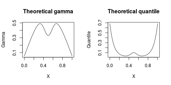
Figure 1: Pattern of $\gamma_{Y}(\cdot)$ and $q(1/1000|\cdot)$ on $[0,1]$ .

The conditional distribution of $C$ given $X=x$ is also Weibull and its parameter $\gamma_{C}(x)$ is chosen to yield three scenarios such as $\gamma_{Y}(x)<\gamma_{C}(x),\gamma_{Y}(x)=\gamma_{C}(x)$ and $\gamma_{Y}(x)>\gamma_{C}(x)$, corresponding to different intensities of censoring in the tail. For each of the $N$ samples, we estimate $\gamma_{Y}(\cdot)$ at different value of $x=(0.1,0.2,0.3,0.4,0.5,0.6,0.7,0.8,0.9)$ for example $x=0.5\quad(\gamma_{Y}(0.5)=0.33)$ using our estimator presented in Equation (20).

In this simulation experiment, we are interest to estimate $\gamma_{Y}(x)$ using the estimators $\hat{\gamma}_{Y}^{(complete)}(x)$, $\hat{\gamma}_{Z}^{(complete)}(x)$ and $\hat{\gamma}_{Y}(x)$, with an asymmetric linear kernel defined as $K(u)=(1.9-1.8u)\mathds{1}_{u\in[-1,1]}$.
Our proposed estimators depend on the bandwidth parameter $h_{n}=h$ which is chosen using a data-driven method since it does not require any prior knowledge about the function $\gamma_{Y}(x)$. However, the bandwidth parameter $h$ is chosen using the cross-validation method which were implemented in Gardes & Girard [2012].

$$h^{opt}=\arg\min_{h_{n}\in\mathcal{H}}\sum_{i=1}^{n}\sum_{j=1}^{n}\left(\mathbb{\textbf{1}}_{\{Z_{i}>Z_{j}\}}-\widehat{\bar{F}}_{n,-i}(Z_{j}|x_{i})\right)^{2},$$

where $\mathcal{H}$ is a grid of values for $h_{n}$ and $\widehat{\bar{F}}_{n,-i}$ is the kernel conditional Kaplan-Meier estimator adapted in Ndao et al. [2016], which depends on parameter $h_{n}$.

In case the bandwidth has already been selected, we adopt the method used in Ndao et al. [2016] to choose the threshold excess $k_{x}=k$ and described as follows:

1. we compute the estimate $\hat{\gamma}_{Y}(x)$ with $k=1,\cdots,n-1$,

2. we form several successive ”blocks” of estimates $\hat{\gamma}_{Y}(x)$ (one block for $k\in\{1,\ldots,10\}$, a second block for $k\in\{11,\ldots,20\}$ and so on),

3. we calculate the standard deviation of the estimates within each block,

4. we determine the $k$-value to be used (thereafter denoted by $k^{*}$) from the block with minimal standard deviation. Precisely, we take the middle value of the $k$-values in the block (see Ndao et al. [2016], Goegebeur et al. [2014a])

In simulation experiences, the choice of kernel density function does not shown any impact in performance of our proposed estimators. By rerun our experiments with other kernel density function for example of a bi-quadratic kernel defined as $K(u)=\frac{15}{16}(1-u^{2})^{2}\mathds{1}_{u\in[-1,1]}$ and there is no impact in the results.

Regarding the estimation of the upper extreme quantile, we performed different experiment by examining the behaviors of $\hat{q}_{w}(1-\alpha_{n}|x)$ with respect to the value of $\hat{\gamma}_{Y}^{(complete)}(x)$, $\hat{\gamma}_{Z}^{(complete)}(x)$ and $\hat{\gamma}_{Y}(x)$ where $\alpha_{n}=1/1000$.

4.2 Results

Table 1 and Table 2 give an overview of the performances of our estimators of the conditional Weibull-tail coefficient $\gamma_{Y}(x)$ and conditional extreme quantile $q(\alpha_{n}|x)$ for small probability $\alpha_{n}$. Based on the value of empirical Mean Squared Error (MSE) and empirical Mean Absolute Error (MAE) over the $N$ estimates, we access the accuracy of our proposed estimators based on the different censoring intensities.

To demonstrate the effectiveness of our estimator $\hat{\gamma}_{Y}(x)$ presented in Equation (20), we also compare it with $\hat{\gamma}^{(comp)}_{Y}(x)$ defined in Equation (19), by considering that the sample $Y$ is observed but practically is wrong, since we can not observed a sample $Y$ in censored framework. Again we make the comparison with $\hat{\gamma}^{(comp)}_{Z}(x)$ which is the same expression as $\hat{\gamma}^{(comp)}_{Y}(x)$ but applied to the observed sample $Z$ instead to sample $Y$. For each experiment, we considered three scenario $\gamma_{Y}(x)<\gamma_{C}(x),\gamma_{Y}(x)=\gamma_{C}(x)$ and $\gamma_{Y}(x)>\gamma_{C}(x)$ .

Table 1 illustrate the different value of empirical MSE and empirical MAE of our estimators of Weibull tail coefficient $\gamma_{Y}(x)$ at different sample size with respect to the different censoring intensities respectively. As expected the simulation study show that an estimator $\hat{\gamma}^{(comp)}_{Z}(x)$ not adapted to censoring framework yields inaccurate results, even in the case $\gamma_{Y}(x)<\gamma_{C}(x)$ , where $\hat{\gamma}^{(comp)}_{Z}(x)$ is consistent for estimating $\gamma_{Y}(x)$.

As illustrated from Table 1, the Hill’s kernel version estimator under censorship proposed estimator presented in Equation (20) of $\gamma_{Z}(x)$ shows to be well performed in almost simulation cases. As result, it performs quite better on the scenario $\gamma_{Y}(x)<\gamma_{C}(x)$ for large enough sample size and its quality becomes worst as $\gamma_{Y}(x)>\gamma_{C}(x)$ and sample size decreases.

According to the Boxplot of the estimators of $\gamma_{Y}(x)$ for $N=500$ random sample of sample size $n=100,300,500$ presented in Figure 2, 3 and 4 for the case $\gamma_{Y}(x)<\gamma_{C}(x)$, $\gamma_{Y}(x)=\gamma_{C}(x)$ and $\gamma_{Y}(x)>\gamma_{C}(x)$ respectively. As expected, the figures show that the proposed estimator for $\gamma_{Y}(x)$ in framework of censorship is well performed for all scenarios as the sample size is large enough.

In Table 2, we present different value of empirical MSE and empirical MAE of our estimators of extreme conditional quantile $q(\cdot|x)$ at different sample size increases with respect to the different censoring intensities respectively. As expected the simulation study show that an estimator correspondent to (here $\hat{\gamma}^{(comp)}_{Z}(x)$) not adapted to censoring yields inaccurate results, even in the case $\gamma_{Y}(x)<\gamma_{C}(x)$.

As illustrated from Table 2, Weissman quantile estimator under censorship proposed estimator presented in Equation (24) of $q(\cdot|x)$ shows to be well performed in almost simulation cases. As result, it performs quite better on the scenario $\gamma_{Y}(x)<\gamma_{C}(x)(x)$ for large enough sample size and its quality becomes worst as $\gamma_{Y}(x)>\gamma_{C}(x)$ and sample size decreases.

According to the Boxplot of the estimators of $q(\cdot|x)$ for $N=500$ random sample of sample size $n=100,300,500$ presented in Figures 5, 6 and 7 for the case $\gamma_{Y}(x)<\gamma_{C}(x)$, $\gamma_{Y}(x)=\gamma_{C}(x)$ and $\gamma_{Y}(x)>\gamma_{C}(x)$ respectively. The result shows that the proposed estimator for $q(\cdot|x)$ in framework of censorship is well performed for all scenarios as the sample size is large enough.

Table 1: simulation results for the estimator of $\gamma_{Y}(x)$: empirical MSE, empirical MAE for $N=500$ replications.

	estimator	$\gamma_{Y}(0.1)=0.2249$		$\gamma_{Y}(0.2)=0.3777$		$\gamma_{Y}(0.3)=0.4823$		$\gamma_{Y}(0.4)=0.4395$		$\gamma_{Y}(0.5)=0.3300$		$\gamma_{Y}(0.6)=0.4395$		$\gamma_{Y}(0.7)=0.4823$		$\gamma_{Y}(0.8)=0.3777$		$\gamma_{Y}(0.9)=0.2249$
$n$		MSE	MAE	MSE	MAE	MSE	MAE	MSE	MAE	MSE	MAE	MSE	MAE	MSE	MAE	MSE	MAE	MSE	MAE
For $\gamma_{Y}<\gamma_{C}$
	$\hat{\gamma}^{(comp)}_{Y}(x)$	0.0019	0.0340	0.0053	0.0565	0.0086	0.0713	0.0081	0.0701	0.0047	0.0529	0.0074	0.0682	0.0085	0.0721	0.0068	0.0644	0.0021	0.0362
100	$\hat{\gamma}_{Z}^{(comp)}(x)$	0.0145	0.1043	0.0437	0.1777	0.0658	0.2188	0.0640	0.2151	0.0315	0.1529	0.0600	0.2108	0.0684	0.2209	0.0400	0.1733	0.0138	0.0982
	$\hat{\gamma}_{Y}(x)$	0.0019	0.0339	0.0047	0.0525	0.0084	0.0719	0.0081	0.0685	0.0038	0.0476	0.0067	0.0640	0.0083	0.0721	0.0058	0.0608	0.0017	0.0329
For $\gamma_{Y}=\gamma_{C}$
	$\hat{\gamma}^{(comp)}_{Y}(x)$	0.0023	0.0376	0.0066	0.0651	0.0116	0.0847	0.0093	0.0744	0.0056	0.0572	0.0105	0.0788	0.01508	0.0952	0.0094	0.0733	0.0032	0.0445
100	$\hat{\gamma}_{Z}^{(comp)}(x)$	0.0024	0.0378	0.0069	0.0644	0.0111	0.0819	0.0101	0.0781	0.0057	0.0580	0.0121	0.0850	0.0155	0.1002	0.0096	0.0764	0.0044	0.0506
	$\hat{\gamma}_{Y}(x)$	0.0020	0.0353	0.0053	0.0560	0.0088	0.0734	0.0076	0.0670	0.0043	0.0506	0.0073	0.0677	0.0099	0.0750	0.0056	0.0576	0.0024	0.0381
For $\gamma_{Y}>\gamma_{C}$
	$\hat{\gamma}^{(comp)}_{Y}(x)$	0.0017	0.0326	0.0048	0.0551	0.0092	0.0748	0.0064	0.0628	0.0045	0.0528	0.0078	0.0697	0.0085	0.0742	0.0058	0.0599	0.0020	0.0362
100	$\hat{\gamma}_{Z}^{(comp)}(x)$	0.0048	0.0632	0.0132	0.1024	0.0211	0.1311	0.0184	0.1216	0.0099	0.0893	0.0197	0.1279	0.0229	0.1329	0.0147	0.1074	0.0051	0.0636
	$\hat{\gamma}_{Y}(x)$	0.0022	0.0372	0.0079	0.0672	0.0119	0.0834	0.0099	0.0763	0.0053	0.0564	0.01028	0.0755	0.0121	0.0869	0.0070	0.0636	0.0029	0.04036
For $\gamma_{Y}<\gamma_{C}$
	$\hat{\gamma}^{(comp)}_{Y}(x)$	0.0006	0.0206	0.0018	0.0345	0.0026	0.0410	0.00229	0.0377	0.00119	0.0274	0.0025	0.0404	0.0028	0.0427	0.0017	0.03377	0.0006	0.0211
300	$\hat{\gamma}_{Z}^{(comp)}(x)$	0.0101	0.0873	0.0277	0.1452	0.0468	0.1923	0.0369	0.1698	0.0213	0.1293	0.0365	0.1643	0.0446	0.1884	0.0268	0.1417	0.0095	0.0860
	$\hat{\gamma}_{Y}(x)$	0.0005	0.0181	0.0015	0.0303	0.0025	0.0402	0.00222	0.0373	0.00112	0.0260	0.0020	0.0341	0.0024	0.0394	0.0016	0.0318	0.0005	0.0182
For $\gamma_{Y}=\gamma_{C}$
	$\hat{\gamma}^{(comp)}_{Y}(x)$	0.00076	0.0218	0.00222	0.0363	0.0032	0.0452	0.0027	0.0417	0.0016	0.0324	0.0031	0.0444	0.0037	0.0478	0.0026	0.0399	0.0011	0.0265
300	$\hat{\gamma}_{Z}^{(comp)}(x)$	0.00075	0.0213	0.00225	0.0377	0.0033	0.0460	0.0029	0.0419	0.0017	0.033	0.0034	0.0457	0.0040	0.0502	0.0027	0.0410	0.0009	0.0239
	$\hat{\gamma}_{Y}(x)$	0.00059	0.0193	0.0017	0.0334	0.0026	0.0412	0.0019	0.0357	0.0013	0.0287	0.0025	0.0391	0.0026	0.0405	0.0017	0.0327	0.0005	0.0185
For $\gamma_{Y}>\gamma_{C}$
	$\hat{\gamma}^{(comp)}_{Y}(x)$	0.0006	0.0195	0.0018	0.0348	0.0034	0.0453	0.0025	0.0410	0.0015	0.0305	0.0032	0.0452	0.0036	0.0470	0.0025	0.0400	0.0009	0.0235
300	$\hat{\gamma}_{Z}^{(comp)}(x)$	0.0038	0.0593	0.0115	0.1029	0.0174	0.1255	0.0147	0.1162	0.0083	0.0874	0.0140	0.1122	0.0165	0.1224	0.0094	0.0914	0.0035	0.0560
	$\hat{\gamma}_{Y}(x)$	0.0007	0.0207	0.0019	0.0343	0.0038	0.0499	0.0024	0.0385	0.0013	0.0295	0.0031	0.0437	0.0033	0.0461	0.0022	0.0361	0.00071	0.0213
For $\gamma_{Y}<\gamma_{C}$
	$\hat{\gamma}^{(comp)}_{Y}(x)$	0.00038	0.0155	0.0012	0.0278	0.0019	0.0355	0.0017	0.0338	0.0008	0.0233	0.0020	0.0360	0.0019	0.0349	0.0014	0.0297	0.0006	0.0199
500	$\hat{\gamma}_{Z}^{(comp)}(x)$	0.0091	0.0831	0.0257	0.1406	0.0405	0.1749	0.0359	0.1657	0.0189	0.1222	0.0354	0.1644	0.0410	0.1721	0.0258	0.1369	0.0096	0.0818
	$\hat{\gamma}_{Y}(x)$	0.00030	0.0138	0.0010	0.0251	0.0015	0.0315	0.0012	0.0271	0.0006	0.0205	0.0012	0.0282	0.0015	0.0305	0.0009	0.0237	0.0003	0.0145
For $\gamma_{Y}=\gamma_{C}$
	$\hat{\gamma}^{(comp)}_{Y}(x)$	0.00040	0.0161	0.00109	0.0261	0.0023	0.0389	0.0016	0.0327	0.0008	0.0234	0.0016	0.0314	0.0022	0.0373	0.0013	0.0284	0.0006	0.0200
500	$\hat{\gamma}_{Z}^{(comp)}(x)$	0.00041	0.0158	0.00109	0.0260	0.0019	0.0351	0.0015	0.0315	0.0009	0.0244	0.0015	0.0307	0.0023	0.0380	0.0013	0.0297	0.0005	0.0188
	$\hat{\gamma}_{Y}(x)$	0.00033	0.0145	0.00102	0.02549	0.0014	0.0308	0.0012	0.0276	0.0007	0.0220	0.0012	0.0274	0.0016	0.0315	0.0009	0.0248	0.0003	0.0151
For $\gamma_{Y}>\gamma_{C}$
	$\hat{\gamma}^{(comp)}_{Y}(x)$	0.0004	0.0162	0.0010	0.0247	0.0019	0.0346	0.0013	0.0295	0.0009	0.0241	0.0015	0.0315	0.0020	0.0365	0.0012	0.0276	0.0004	0.0167
500	$\hat{\gamma}_{Z}^{(comp)}(x)$	0.0040	0.0624	0.011	0.1057	0.0183	0.1318	0.0151	0.1199	0.0085	0.0900	0.0148	0.1187	0.0181	0.1309	0.0105	0.0998	0.0038	0.0600
	$\hat{\gamma}_{Y}(x)$	0.0004	0.0162	0.0012	0.0277	0.0021	0.0359	0.0018	0.0345	0.0009	0.0240	0.0018	0.0342	0.0017	0.0339	0.0014	0.0296	0.0004	0.0166

Figure 2: Pattern simulation for $N=500$ of estimates of $\gamma_{Y}(\cdot)$ on $[0,1]$ with $n=100$ first line, $n=300$ second line, $n=500$. Left $\hat{\gamma}_{Y}(x)$, center $\hat{\gamma}^{(comp)}_{Z}(x)$ and right $\hat{\gamma}^{(comp)}_{Y}(x)$ where $\gamma_{Y}<\gamma_{C}$.

Figure 3: Pattern simulation for $N=500$ of estimates of $\gamma_{Y}(\cdot)$ on $[0,1]$ with $n=100$ first line, $n=300$ second line, $n=500$. Left $\hat{\gamma}_{Y}(x)$, center $\hat{\gamma}^{(comp)}_{Z}(x)$ and right $\hat{\gamma}^{(comp)}_{Y}(x)$ where $\gamma_{Y}>\gamma_{C}$.

Figure 4: Pattern simulation for $N=500$ of estimates of $\gamma_{Y}(\cdot)$ on $[0,1]$ with $n=100$ first line, $n=300$ second line, $n=500$. Left $\hat{\gamma}_{Y}(x)$, center $\hat{\gamma}^{(comp)}_{Z}(x)$ and right $\hat{\gamma}^{(comp)}_{Y}(x)$ where $\gamma_{Y}=\gamma_{C}$.

Table 2: Simulation results for the estimator of $q(\alpha_{n}|\cdot)$ where $\alpha_{n}=1/1000$: empirical MSE and empirical MAE for $N=500$ replications.

	estimator	$q(\alpha_{n}|0.1)=0.2114$		$q(\alpha_{n}|0.2)=0.0735$		$q(\alpha_{n}|0.3)=0.0357$		$q(\alpha_{n}|0.4)=0.0480$		$q(\alpha_{n}|0.5)=0.1023$		$q(\alpha_{n}|0.6)=0.0480$		$q(\alpha_{n}|0.7)=0.0357$		$q(\alpha_{n}|0.8)=0.0735$		$q(\alpha_{n}|0.9)=0.2114$
$n$		MSE	MAE	MSE	MAE	MSE	MAE	MSE	MAE	MSE	MAE	MSE	MAE	MSE	MAE	MSE	MAE	MSE	MAE
For $\gamma_{Y}<\gamma_{C}$
	$\hat{\gamma}^{(comp)}_{Y}(x)$	0.0037	0.0453	0.0012	0.0256	0.0004	0.0152	0.0007	0.0197	0.0016	0.0313	0.0006	0.0193	0.00039	0.0145	0.0011	0.0259	0.0037	0.0449
100	$\hat{\gamma}_{Z}^{(comp)}(x)$	0.0093	0.0813	0.0018	0.0384	0.0005	0.0206	0.0009	0.0262	0.0032	0.0499	0.0009	0.0273	0.00054	0.0206	0.0019	0.0381	0.0090	0.0796
	$\hat{\gamma}_{Y}(x)$	0.0033	0.0425	0.0008	0.0220	0.0003	0.0144	0.0006	0.0182	0.0013	0.0286	0.0006	0.0181	0.00035	0.0139	0.0010	0.0243	0.0031	0.0421
For $\gamma_{Y}=\gamma_{C}$
	$\hat{\gamma}^{(comp)}_{Y}(x)$	0.0040	0.0496	0.00108	0.0263	0.00048	0.0158	0.00059	0.0193	0.0019	0.0346	0.0007	0.0212	0.00048	0.0169	0.0012	0.0279	0.0044	0.0545
100	$\hat{\gamma}_{Z}^{(comp)}(x)$	0.0037	0.0484	0.00105	0.0258	0.00046	0.0164	0.00059	0.0198	0.0016	0.0337	0.0006	0.0201	0.00048	0.0170	0.0011	0.0278	0.0047	0.0560
	$\hat{\gamma}_{Y}(x)$	0.0034	0.0456	0.00103	0.0265	0.00039	0.0157	0.00070	0.0199	0.0017	0.0324	0.0007	0.0201	0.00044	0.0160	0.0009	0.0252	0.0034	0.0455
For $\gamma_{Y}>\gamma_{C}$
	$\hat{\gamma}^{(comp)}_{Y}(x)$	0.0038	0.0485	0.0012	9 0.0275	0.0006	0.0182	0.0008	0.0214	0.0020	0.0357	0.0009	0.0231	0.0006	0.0189	0.0016	0.0308	0.0044	0.0519
100	$\hat{\gamma}_{Z}^{(comp)}(x)$	0.0151	0.1025	0.0077	0.0697	0.0040	0.0497	0.0056	0.0595	.0096	0.0806	0.0066	0.0663	0.0047	0.0531	0.0096	0.0776	0.0165	0.1071
	$\hat{\gamma}_{Y}(x)$	0.0039	0.0505	0.0012	0.0283	0.0006	0.0186	0.0007	0.0215	0.0018	0.0337	0.0008	0.0220	0.0005	0.0183	0.0015	0.0306	0.0046	0.0531
For $\gamma_{Y}<\gamma_{C}$
	$\hat{\gamma}^{(comp)}_{Y}(x)$	0.0015	0.0275	0.0004	0.0155	0.0001	0.0091	0.0002	0.0107	0.0005	0.0169	0.0002	0.0115	0.00015	0.0094	0.0004	0.0150	0.0013	0.0278
300	$\hat{\gamma}_{Z}^{(comp)}(x)$	0.0067	0.0723	0.0015	0.0353	0.0004	0.0199	0.0007	0.0251	0.0027	0.0471	0.0007	0.0246	0.0004	0.0197	0.0014	0.0338	0.0066	0.0714
	$\hat{\gamma}_{Y}(x)$	0.0010	0.0236	0.0003	0.0136	0.0001	0.0088	0.0002	0.0110	0.0005	0.0172	0.0001	0.0101	0.0001	0.0084	0.0003	0.0145	0.0009	0.0242
For $\gamma_{Y}=\gamma_{C}$
	$\hat{\gamma}^{(comp)}_{Y}(x)$	0.0012	0.0272	0.00041	0.0160	0.0001	0.0096	0.000198	0.0115	0.0006	0.0194	0.00023	0.0122	0.00013	0.0093	0.00040	0.0162	0.0015	0.0326
300	$\hat{\gamma}_{Z}^{(comp)}(x)$	0.0012	0.0272	0.00044	0.0165	0.0001	0.0093	0.000194	0.0113	0.00056	0.0192	0.00023	0.0126	0.00015	0.0102	0.00044	0.0173	0.0014	0.0303
	$\hat{\gamma}_{Y}(x)$	0.0011	0.0258	0.00040	0.0154	0.0001	0.0093	0.0002	0.0110	0.00051	0.0180	0.00021	0.0114	0.00013	0.0089	0.00041	0.0157	0.0010	0.0253
For $\gamma_{Y}>\gamma_{C}$
	$\hat{\gamma}^{(comp)}_{Y}(x)$	0.0011	0.0264	0.00040	0.0160	0.00016	0.0098	0.00023	0.0121	0.00061	0.0194	0.00023	0.0126	0.00013	0.0092	0.00044	0.0170	0.0014	0.0303
300	$\hat{\gamma}_{Z}^{(comp)}(x)$	0.0104	0.0936	0.0054	0.0671	0.00236	0.0429	0.0033	0.0519	0.0067	0.0748	0.0031	0.0494	0.0022	0.0415	0.0041	0.0571	0.0094	0.0866
	$\hat{\gamma}_{Y}(x)$	0.0012	0.0286	0.00043	0.0163	0.00019	0.011	0.00026	0.0123	0.00064	0.0198	0.00030	0.0132	0.00017	0.0103	0.00045	0.0169	0.0013	0.0293
For $\gamma_{Y}<\gamma_{C}$
	$\hat{\gamma}^{(comp)}_{Y}(x)$	0.0007	0.0196	0.0002	0.0122	9.6e-05	0.0074	0.00013	0.0092	0.0003	9 0.0138	0.00014	0.0093	8.6e-05	0.0072	0.00029	0.0132	0.0009	0.0239
500	$\hat{\gamma}_{Z}^{(comp)}(x)$	0.0066	0.0731	0.0015	0.0361	4.7e-04	0.0200	0.00079	0.0260	0.0025	0.0451	0.00077	0.0255	4.2e-04	0.0183	0.00136	0.0322	0.0063	0.0706
	$\hat{\gamma}_{Y}(x)$	0.0006	0.0196	0.0002	0.0119	8.7e-05	0.0072	0.00011	0.0083	0.0003	0.0140	0.00011	0.0082	7.4e-05	0.0066	0.00021	0.0113	0.0007	0.0195
For $\gamma_{Y}=\gamma_{C}$
	$\hat{\gamma}^{(comp)}_{Y}(x)$	0.00069	0.0210	0.0002	0.0118	1.0e-04	0.0084	0.00013	0.0092	0.0003	0.0146	0.00012	0.0088	1.0e-04	0.0081	0.00025	0.0125	0.0009	0.0252
500	$\hat{\gamma}_{Z}^{(comp)}(x)$	0.00072	0.0208	0.0002	0.0118	9.0e-05	0.0076	0.00012	0.0090	0.0003	0.0152	0.00012	0.0087	8.9e-05	0.0077	0.00025	0.0128	0.0009	0.0236
	$\hat{\gamma}_{Y}(x)$	0.00062	0.0198	0.0002	0.0120	8.1e-05	0.0071	0.00012	0.0086	0.0003	0.0146	0.00011	0.0082	8.2e-05	0.0070	0.00020	0.0114	0.0006	0.0209
For $\gamma_{Y}>\gamma_{C}$
	$\hat{\gamma}^{(comp)}_{Y}(x)$	0.0007	0.0217	0.0002	0.0115	9.71e-05	0.0077	0.0001	0.0092	0.0003	0.0149	0.0001	0.0095	1.06e-04	0.0080	0.0002	0.0124	0.0007	0.0226
500	$\hat{\gamma}_{Z}^{(comp)}(x)$	0.0104	0.0964	0.0051	0.0666	2.1e-03	0.0445	0.0032	0.0530	0.0065	0.0753	0.0031	0.0523	2.4e-03	0.0449	0.0045	0.0633	0.0102	0.0945
	$\hat{\gamma}_{Y}(x)$	0.0008	0.0225	0.0002	0.0132	1.05e-04	0.0078	0.0001	0.0104	0.0003	0.0153	0.0001	0.0104	9.4e-05	0.0075	0.0003	0.0138	0.0007	.0218

Figure 5: Pattern simulation for $N=500$ of estimates of $q(1/1000|\cdot)$ on $[0,1]$ with $n=100$ first line, $n=300$ second line, $n=500$. For each $\hat{q}_{w}(1/1000|\cdot)$ corresponding to left by $\hat{\gamma}_{Y}(x)$, center by $\hat{\gamma}^{(comp)}_{Z}(x)$ and right by $\hat{\gamma}^{(comp)}_{Y}(x)$ where $\gamma_{Y}<\gamma_{C}$.

Figure 6: Pattern simulation for $N=500$ of estimates of $q(1/1000|\cdot)$ on $[0,1]$ with $n=100$ first line, $n=300$ second line, $n=500$. For each $\hat{q}_{w}(1/1000|\cdot)$ corresponding to left by $\hat{\gamma}_{Y}(x)$, center by $\hat{\gamma}^{(comp)}_{Z}(x)$ and right by $\hat{\gamma}^{(comp)}_{Y}(x)$ where $\gamma_{Y}>\gamma_{C}$.

Figure 7: Pattern simulation for $N=500$ of estimates of $q(1/1000|\cdot)$ on $[0,1]$ with $n=100$ first line, $n=300$ second line, $n=500$. For each $\hat{q}_{w}(1/1000|\cdot)$ corresponding to left by $\hat{\gamma}_{Y}(x)$, center by $\hat{\gamma}^{(comp)}_{Z}(x)$ and right by $\hat{\gamma}^{(comp)}_{Y}(x)$ where $\gamma_{Y}=\gamma_{C}$.

5 Illustration on real data

The main goal of this section is to illustrate our methodology on real dataset of men suffering from a larynx cancer. According to the literature, this dataset was previously analyzed by Worms & Worms [2019], where the authors considered $Z$ as the time to death if $\delta=1$ or on-study time if $\delta=0$ in months. The comparison of our results with the existence results in literature will be considered. The dataset contains $n=90$ male patients diagnosed with a larynx cancer, the dataset is available and fully presented in John P. Klein [2005]. Gomes & Neves [2011] introduced the aspect of the estimation of extreme values using this datasets. The information on each patient includes the time on study in month, the age at diagnosis, the age of diagnosed, stage of disease as indicator which equals $1$ if the patient died and 0 otherwise. In this dataset $50$ patients died; the other survival times are right-censored. Worms & Worms [2019] estimated the extreme value index $\gamma_{Y}$ and Weissman extreme quantile (with $\alpha_{n}=0.05$) of the (unconditional) distribution $\bar{F}_{y}(\cdot)$ of the survival time $Y$, then they considered $k_{n}=37$ which gives $\hat{x}_{p}(0.05)=22$ as presented in Worms & Worms [2019].

The Weibull quantile-quantile plots for the data is considered, we plot the points $(\log\log(n/i)$, $\log(Z_{n-i+1,n}))$, for $i=1,\cdots,k_{n}$ , for well chosen value of $k_{n}$ the graphical presentation is illustrated in Figure 8 to support the assumption that a Weibull-tail distribution is a possible to the dataset of men suffering from a larynx cancer. The remaining challenge is the right choice of the $k_{n}$ and $h$. In this section, to determine optimum values of $h$ and threshold excess $k$, we use the same methods as mentioned in Section 4.1.
By taking into consideration of the presence of covariate and using the aforementioned strategy to determine the appropriate value of $k$, we get $k=54$.

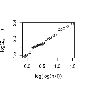
Figure 8: Weibull Quantile-Quantile for $k_{n}=54$ with dataset of men suffering from a larynx cancer .

We rerun these data, taking account of the age at diagnosis denoted by x in what follows. For illustration of our proposed estimator, We estimate the quantile $q(0.05|x)$ of order $1-0.05$ of the conditional distribution of $Z$ given $x$ for the case $x=65$ (median of the $(x,\cdots,x_{n})$, $x=54.20\;(median-sd(x_{1},\cdots,x_{n}))$ and $x=75.80\;(median+sd(x_{1},\cdots,x_{n}))$ where $sd(x_{1},\cdots,x_{n}$ is the empirical standard deviation of $x_{1},\cdots,x_{n}$. The results are presented in Table 3.

Table 3: Estimation of the Weibull-tail coefficient and conditional extreme quantile, first column: $median(x)-sd(x)$, second column: $median(x)$ and third column: $median(x)+sd(x)$.

x	54.20	65	75.80
For $k=54$
$\hat{\gamma}_{Y}(x)$	0.8219978	0.8225810	0.8210728
$\hat{q}_{w}(0.05|x)$	17.6013366	17.6222551	17.5682097
For $k=37$
$\hat{\gamma}_{Y}(x)$	1.0164362	1.017575	1.0146309
$\hat{q}_{w}(0.05|x)$	23.1668062	23.209382	23.0994800

Finally, from Table 3, we observe that for every $x$ the estimates (24) are smaller than the unconditional estimate obtained by Worms & Worms [2019], thus providing less optimistic perspectives for being infected. But we expect our results to be more representative of the real chance of being survive of these larynx cancer patients, since our analysis takes account of the influent variable ”age at diagnosis”.

6 Conclusion and Perspectives

In this paper, the estimation of the Weibull tail coefficient and extreme quantiles of a Weibull tail type distribution when some covariate information is available and the data are randomly right-censored are considered. The proposed estimators for conditional Weibull tail coefficient and conditional Weissman quantile are derived. The parameter estimation method is proposed to prove its performance. We assessed their finite-sample performance via simulations. A comparison with two estimation strategies has been provided. Our intensive simulation study shows that the proposed estimators are competitive in all scenario as the sample size becomes large enough.

A future possible work would be to exploit our proposed methodology in presence of functional random covariate. Some additional research is needed to establish asymptotic normality of our proposed estimators.

References

References

- Beirlant et al. [1996] Beirlant, J., Teugels, J. L., & Vynckier, P. (1996). Practical analysis of extreme values volume 50. Leuven University Press Leuven.
- Beirlant et al. [2004] Beirlant, J., Yuri, G., Jozef, T., Johan, S., Daniel, D. W., & Chris, F. (2004). Statistics of extremes. John Wiley & Sons Ltd, 10, 151–174.
- Berred [1991] Berred, M. (1991). Record values and the estimation of the weibull tail-coefficient. Comptes rendus de l’Académie des sciences. Série 1, Mathématique, 312, 943–946.
- Cabras & Castellanos [2011] Cabras, S., & Castellanos, M. E. (2011). A bayesian approach for estimating extreme quantiles under a semiparametric mixture model. ASTIN Bulletin, 41, 87–106. doi:10.2143/AST.41.1.2084387.
- Coles & Powell [1996] Coles, S. G., & Powell, E. A. (1996). Bayesian methods in extreme value modelling: a review and new developments. International Statistical Review/Revue Internationale de Statistique, (pp. 119–136).
- Diebolt et al. [2008] Diebolt, J., Gardes, L., Girard, S., & Guillou, A. (2008). Bias-reduced extreme quantile estimators of weibull tail-distributions. Journal of Statistical Planning and Inference, 138, 1389–1401.
- Fisher & Tippett [1928] Fisher, R. A., & Tippett, L. H. C. (1928). Limiting forms of the frequency distribution of the largest or smallest member of a sample. Mathematical Proceedings of the Cambridge Philosophical Society, 24, 180–190. doi:10.1017/S0305004100015681.
- Gardes & Girard [2012] Gardes, L., & Girard, S. (2012). Functional kernel estimators of large conditional quantiles. Electronic Journal of Statistics, 6, 1715–1744.
- Gardes & Girard [2016] Gardes, L., & Girard, S. (2016). On the estimation of the functional weibull tail-coefficient. Journal of Multivariate Analysis, 146, 29–45.
- Goegebeur et al. [2014a] Goegebeur, Y., Guillou, A., & Osmann, M. (2014a). A local moment type estimator for the extreme value index in regression with random covariates. Canadian Journal of Statistics, 42, 487–507.
- Goegebeur et al. [2014b] Goegebeur, Y., Guillou, A., & Schorgen, A. (2014b). Nonparametric regression estimation of conditional tails: the random covariate case. Statistics, 48, 732–755.
- Gomes & Neves [2011] Gomes, M. I., & Neves, M. M. (2011). Estimation of the extreme value index for randomly censored data. Biometrical Letters, 48, 1–22.
- John P. Klein [2005] John P. Klein, M. L. M. (2005). Survival Analysis: Techniques for Censored and Truncated Data. Statistics for Biology and Health (2nd ed.). Springer. URL: http://gen.lib.rus.ec/book/index.php?md5=8a70c414ede17984621958bdc45688e0.
- Matthys et al. [2004] Matthys, G., Delafosse, E., Guillou, A., & Beirlant, J. (2004). Estimating catastrophic quantile levels for heavy-tailed distributions. Insurance: Mathematics and Economics, 34, 517–537.
- Nadaraya [1964] Nadaraya, E. A. (1964). On estimating regression. Theory of Probability & Its Applications, 9, 141–142.
- Ndao [2015] Ndao, P. (2015). Modélisation de valeurs extrêmes conditionnelles en présence de censure. PhD thesis, Université Gaston Berger de Saint-Louis.
- Ndao et al. [2014] Ndao, P., Diop, A., & Dupuy, J.-F. (2014). Nonparametric estimation of the conditional tail index and extreme quantiles under random censoring. Computational Statistics & Data Analysis, 79, 63–79.
- Ndao et al. [2016] Ndao, P., Diop, A., & Dupuy, J.-F. (2016). Nonparametric estimation of the conditional extreme-value index with random covariates and censoring. Journal of Statistical Planning and Inference, 168, 20–37.
- Stephenson & Tawn [2004] Stephenson, A., & Tawn, J. (2004). Bayesian inference for extremes: accounting for the three extremal types. Extremes, 7, 291–307.
- Stupfler [2016] Stupfler, G. (2016). Estimating the conditional extreme-value index under random right-censoring. Journal of Multivariate Analysis, 144, 1–24.
- Watson [1964] Watson, G. S. (1964). Smooth regression analysis. Sankhyā: The Indian Journal of Statistics, Series A, (pp. 359–372).
- de Wet et al. [2016] de Wet, T., Goegebeur, Y., Guillou, A., & Osmann, M. (2016). Kernel regression with weibull-type tails. Annals of the Institute of Statistical Mathematics, 68, 1135–1162.
- Worms & Worms [2014] Worms, J., & Worms, R. (2014). New estimators of the extreme value index under random right censoring, for heavy-tailed distributions. Extremes, 17, 337–358.
- Worms & Worms [2019] Worms, J., & Worms, R. (2019). Estimation of extremes for weibull-tail distributions in the presence of random censoring. Extremes, 22, 667–704.