Accurate effective harmonic potential treatment of the high-temperature cubic phase of Hafnia
Abstract
\ceHfO_2 is an important high- dielectric and ferroelectric, exhibiting a complex potential energy landscape with several phases close in energy. It is, however, a strongly anharmonic solid, and thus describing its temperature-dependent behavior is methodologically challenging. We propose an approach based on self-consistent, effective harmonic potentials and higher-order corrections to study the potential energy surface of anharmonic materials. The introduction of a reweighting procedure enables the usage of unregularized regression methods and efficiently harnesses the information contained in every data point obtained from density functional theory. This renders the approach highly efficient and a promising candidate for large-scale studies of materials and phase transitions. We detail the approach and test it on the example of the high-temperature cubic phase of \ceHfO_2. Our results for the thermal expansion coefficient, , are in agreement with existing experimental () and theoretical () work. Likewise, the bulk modulus agrees well with experiment. We show the detailed temperature dependence of these quantities.
I Introduction
One of the biggest drawbacks of density functional theory (DFT) calculations is the lack of temperature-induced effects. However, due to the exponential growth in computing power and continuous methodological developments, the previously prohibitively expensive calculations necessary to remedy that shortcoming are becoming viable for the investigation of new materials. Consequently, the inclusion of temperature is a prominent theme in many current computational efforts Xie et al. (1999); Grabowski et al. (2007); Souvatzis et al. (2008); Grabowski et al. (2009); Hellman et al. (2011, 2013); van Roekeghem et al. (2021); Ehsan et al. (2021).
In the present study we focus on hafnia, \ceHfO_2, which has a multi-faceted phase diagram Tobase et al. (2018) and numerous industrially relevant applications, ranging from a high- gate dielectric for semiconductors in its amorphous Wilk et al. (2001) and (more recently suggested) tetragonal phase Fischer and Kersch (2008), to a ferroelectric in its orthorhombic states Böscke et al. (2011) for e. g. nonvolatile memory applications Müller et al. (2015).
An accurate DFT treatment of its temperature-dependent behavior has proven difficult to achieve in previous theoretical efforts Huan et al. (2014). In the simplest approach, the effect of temperature is included by means of the harmonic approximation (HA), where the phonon modes of the system are described as independent harmonic oscillators. The second-order interatomic force constants (IFCs) are obtained by applying small displacements and mapping the corresponding forces induced by them. However, in the case of structures governed by anharmonic potential energy surfaces (PES), the HA might yield imaginary frequencies, thus indicating mechanical instability, even when experiments confirm the existence of those structures.
Ab-initio molecular dynamics (AIMD) approaches Iftimie et al. (2005) can, in principle, treat such temperature-stabilized structures, but obtaining the free energy of reasonably complex systems through thermodynamic integration proves to be a resource-intensive task and quickly becomes intractable. Moreover, AIMD treats the nuclear motion in a completely classical fashion, and therefore cannot capture effects such as zero-point motion, which can be relevant for e.g. accurately describing the vibrations of light and strongly bonded atoms.
An emerging category of alternatives to AIMD can be labelled as effective harmonic potentials (EHP). The idea goes back to 1955 Hooton (1955) and in essence involves determining the best HA to the part of the PES which dominates nuclear motion. Temperature dependent contributions to the free energy are then included using independent harmonic oscillators based on these EHPs. EHPs have proven to be a rich starting point for understanding temperature dependent behavior using ab-initio methods and, as computational power has become available, prompted various implementations and formulations of the underlying theory Souvatzis et al. (2008); Hellman et al. (2013); Errea et al. (2013); Tadano and Tsuneyuki (2015); Stern and Madsen (2016); van Roekeghem et al. (2021); Monacelli et al. (2021). The implementations mainly differ in how the PES is sampled with methods including stochastic sampling and molecular dynamics trajectories as well as how the deviation between the EHP and the PES is accounted for.
In the present study we focus on the high-temperature cubic (Fmm) hafnia phase (c-\ceHfO_2). c-\ceHfO_2 is an example of a temperature stabilized structure where the small displacement HA yields imaginary frequencies Huan et al. (2014). We show how the use of reweighting in combination with unregularized regression can be employed to obtain the temperature-dependent EHP. Furthermore, the correction for the deviation between the EHP and the true DFT PES is discussed in detail. We compare our results to the available AIMD calculations and experiments.
II Method
II.1 Background
A system described by a Hamiltonian is in a state of thermal equilibrium at constant volume, temperature and number of particles when its free energy
| (1) |
is at a minimum. This equilibrium state is described by a particular quantum mechanical density matrix, , which, were it known, would provide access to the whole thermodynamics of the system. However, it is impossible for all but trivial model systems to solve this problem exactly.
The EHP can be formulated as a variational problem Errea et al. (2014); Monacelli et al. (2021) where a trial density matrix, , which exactly solves a corresponding trial Hamiltonian, , is introduced. differs from the true Hamiltonian only by the form of the potential energy operator , as opposed to . Minimizing the free energy with respect to the trial density matrix is guaranteed by the Gibbs-Bogoliubov inequality Isihara (1968) to provide an upper bound on the free energy
| (2) |
In the harmonic approximation, the trial potential is parametrized as
| (3) |
in terms of the displacements from the minimum-energy configuration, , and the second-order force constants, , whose eigenvalues and eigenvectors
| (4) |
will hereafter be denoted by and . The indices denote the ions and the Cartesian directions. Within the harmonic approximation, the projection onto real space of the trial density matrix can be expressed in closed form
| (5) |
The covariance matrix can be obtained from the aforementioned and through a well-known result of quantum statistical mechanics
| (6) |
where correspond to the masses of the ions. Furthermore, the expression for the free energy, , is given by
II.2 Temperature-dependent effective potentials
We implement the search for the optimal EHP by approximating the real-space density matrix by means of canonical importance sampling and treating the interdependence of and as a self-consistent problem. When self consistency is reached, this corresponds to minimizing van Roekeghem et al. (2021).
The starting point is the second-order force-constant matrix, and corresponding potential , obtained through small displacements as implemented in Phonopy Togo and Tanaka (2015). From the eigenvalues and eigenvectors and the temperature of interest the associated trial density, , is obtained through Eqs. 5 and 6. We replace the imaginary square roots of possible negative eigenvalues from intermediate steps with their modulus. From this probability density the first set of displacements, , are drawn. A new EHP is obtained by calculating the potential energies and forces corresponding to the displacements using DFT and finding the parametrization of the force constants in Eq. 4 which best represent the relationship between forces and displacements, as will be discussed below. The iterative process then progresses by contructing a new density matrix using Eqs. 6 and 5. To aid convergence, the new trial density matrix, , is obtained through a Pulay mixing scheme Pulay (1982) with a memory of and a mixing parameter of , as commonly used. A new set of displacements is now drawn and the process continues until convergence is reached.
To efficiently use all the data obtained from DFT, the reweighting factor Errea et al. (2013) is introduced
| (8) |
Thereby displacement vectors, , belonging to a set drawn in a previous iteration, , and their corresponding forces and potential energies can be included as if they belong to the current set, .
Using the reweighting factors significantly increases the amount of available data and allows using an unregularized fitting procedure to obtain the force constant matrix. The trial potential for iteration is found by finding the force constants which minimize the weighted sum of the least-squares deviations from the calculated forces, i. e. ,
| (9) |
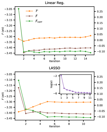
In Fig. 1 the free energy evaluated according to Eq. 7 is shown as a function of the iterations until convergence for the equilibrium volume using a temperature of . Typically the convergence criterion of is reached in iterations when 5 structures are added per iteration for the initial temperature point, totaling 50 - 75 DFT runs.
Alternatively, a penalty
| (10) |
can be defined. This is known as the LASSO minimization target function. The parameter determines the strength of the regularization and promotes sparsity of the force constant matrix, which can be a computational advantage Fransson et al. (2020). By partitioning the data into five complementary subsets and minimizing Eq. 10 for a range of -values, the regularization strength can be tuned to provide the model which generalizes best, i.e. has the best performance on the subsets not used for obtaining the force constants. This so-called 5-fold cross validation procedure Pedregosa et al. (2011) is performed at every step of the iteration. In Fig. 1 we compare the convergence behaviour at for the equilibrium structure. Notably, the parameter quickly approaches zero as the calculation progresses. This is understandable as regularization is typically applied when fitting samples which insufficiently cover the sample space. Thus, as the amount of data points available for fitting increases, every fold in the cross validation procedure will be more and more equally representative of the rest, so the penalty will actually hinder minimizing Eq. 10 and will be forced towards zero by the algorithm itself, effectively resulting in Eq. 9.
We have chosen the unregularized least-squares approach, Eq. 9 for two reasons: We are, for all but the first few iterations, confronted with an overdetermined system, as only a total of independent force constants remain after considering symmetry and the cut-off and every sample provides force-displacement pairs. Furthermore, if a non-zero -penalty was indeed used throughout the calculation, the force constants obtained would not fulfill the property of minimizing the free energy once self-consistency is reached van Roekeghem et al. (2021). As argued above, the regularization parameter must approach zero, because the coverage increases with every iteration. While we would presumably not have arrived at an artificially increased free energy, using LASSO only provided a minor speed up, while introducing additional uncertainty in the results.
The correction term, , has previously been calculated by representing the DFT PES by a simpler form Errea et al. (2013); Monacelli et al. (2021) or by using the trajectory obtained from AIMD Hellman et al. (2013); Metsanurk and Klintenberg (2019). We calculate directly from the DFT potential energies obtained from the same sampling as used for determining the trial EHP, Eq. 9, as a weighted average
| (11) |
where is the sum of all the weights. Similar to the EHP the reweighting allows all DFT calculations to be used for obtaining and Fig. 1 illustrates that the convergence is also comparable, meaning that convergence of the total free energy, , is reached within iterations.
It is straightforward to extend the formalism described above to reuse samples drawn at temperature for a different temperature , by building reweighting factors accounting for this. This provides a fast way to calculate force constants at temperatures near . At temperatures more different from the sample set might not be adequate anymore, necessitating augmentation by additional DFT runs. As an example we mention that using the displacements and forces obtained for , Fig. 1, at , but reweighted according to Eq. 8 results in convergence after adding only two additional iterations. Once convergence has been obtained for a mesh of temperatures, free energies can be obtained at intermediate temperatures without additional DFT calculations. As a measure for when additional calculations are necessary, we use the effective number of samples,
| (12) |
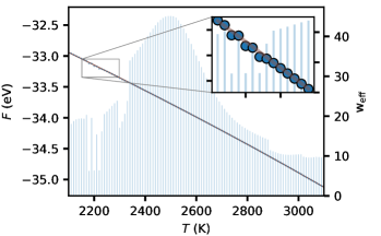
As can be observed in in Fig. 2, the number of effective samples is indeed an excellent metric for the trustworthiness of the data at a given temperature. However, it would be grossly inefficient to augment the data if the poorly-sampled regions are small and constrained and the surrounding points are described by the existing samples well-enough. To prevent this, we apply a smoothing spline weighted with the effective samples to . This procedure avoids artifactual oscillations in later results.
II.3 Computational details
The DFT calculations were performed using the Vienna Ab Initio Simulation Package (VASP) Kresse and Furthmüller (1996); Blöchl (1994); Kresse and Joubert (1999), where we utilized the Perdew-Berke-Ernzerhof (PBE) exchange and correlation potential Perdew et al. (1996) along with an energy cutoff of . The force calculations for the phonons were performed in a supercell using just the -point. We used Phonopy Togo and Tanaka (2015) with the non-analytical correction described in Wang et al. (2010) for obtaining the initial small displacements force constants. The descriptors for fitting the force constants [Eq. 9 and Eq. 10] are obtained using scikit-learn Pedregosa et al. (2011) and the cluster formalism established in Ref. Eriksson et al., 2019 given a pre-defined cutoff .
We performed the steps outlined above for various deformations of the equilibrium structure; we included volumes from , as well as various temperatures ranging from . To arrive at a simple but general analytical expression we then fit the free energies using,
| (13) |
achieving an average deviation between actual and fitted free energy of less than , which corresponds to less than . This allows for finding the equilibrium lattice parameter and volume at every temperature point of interest with a high accuracy.
III Results
We settled on a temperature range from to ensure full coverage of the stable region of c-\ceHfO_2, Wang et al. (2006), with the upper bound close to the melting temperature. To accurately treat this temperature range, we performed an initial self-consistent run at , augmented it with samples at and, guided by the effective sample size, Eq. 12, included for some deformations.
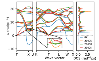
As an example, we show the phonon band structure of the equilibrium structure in Fig. 3, as obtained using small displacements and using the EHP at elevated temperatures. As can be seen c-\ceHfO_2 shows an instability in the small displacements () phonon spectrum at in the Brillouin zone, which, in the structurally very similar \ceZrO_2 has been linked to the cubic-to-tetragonal phase transition Kuwabara et al. (2005). Within the studied temperature range, we see a continuous hardening (shown in the inset) of said mode indicating that temperature-induced anharmonic effects are stabilizing this phase. For the additional volumes that were studied ( volume changes) we find a similar behaviour and can report stable phonon spectra for the whole volume and temperature range.
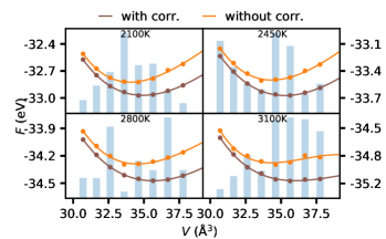
The absence of imaginary phonon frequencies make it possible to calculate the vibrational contribution to the free energy according to Eq. 7. Fig. 4 depicts the volume dependence of the free energy at four different temperatures. Eq. 13, captures the behavior of c-\ceHfO_2 across the studied temperature range and as expected the equilibrium volume increases with temperature. Interestingly, not only shifts the curve to lower energies, , but it also changes the positions of the minima. As expected, gets larger with temperature, i. e. with increasing anharmonic contributions to the relevant parts of the PES. As a result, the contribution generally favors larger volumes and can be expected to be important for a correct predicting of thermal expansion.
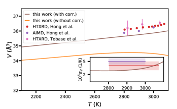
The role of the correction term becomes even more apparent when looking at the thermal expansion in Fig. 5. Comparing the unit-cell volume of c-\ceHfO_2 with experimental and theoretical results from literature, Hong et al. (2018); Tobase et al. (2018) illustrates how neglecting will provide underestimated unit cell volume in situations where anharmonicities contribute a significant portion of the total energy. Such situations can arise when describing materials that are inherently anharmonic, or generally for materials at elevated temperatures. \ceHfO_2 is in our study subject to both of these circumstances and thus any description not taking the anharmonic correction into account is bound to lead to inaccurate conclusions. Even when is included, a constant offset of about , or , can be observed. This can be attributed to inherent approximations of the chosen DFT functional. It is not possible to prove this as no experimental data exists to compare with. However, it is worth noting that the AIMD study reported in Ref. Hong et al., 2018 (employing the same PBE functional), also finds slightly lower volumes than experiment.
The calculated thermal expansion coefficient [see inset in Fig. 5] is approximately constant, , until an increase in thermal expansion can be seen as the melting temperature, , is approached. The thermal expansion coefficient is not impacted by a small constant offset, and our results are within or very close to the uncertainty, indicated by a red bar, of the experimental average over the range from , , obtained by Hong. et al. Hong et al. (2018). The volume data from Tobase et. al Tobase et al. (2018) would result in , over the region of approximately . However, due to the large uncertainty in the volume measurements, the error bar would span about , and hence it is not shown in the graph.
Finally, we report the temperature dependence of the c-\ceHfO_2 bulk modulus. Due to the fact that the second derivative of Eq. 13 w.r.t. lattice parameter (or volume) is not linear, the bulk modulus obtained by our method is naturally dependent on the volume at a given pressure at which it is evaluated. Evaluated at we find a bulk modulus of , which decreases to over the range of . This drastic softening is expected as we are approaching the melting point of the material. In their recent study, Irshad et al. Irshad et al. (2020), have measured the bulk modulus of pressure-stabilized, nanocrystalline c-\ceHfO_2 at ambient temperature, finding . Applying a small pressure of (corresponding to a volume change of ) to our result, yields a comparable bulk modulus of about at , decreasing to at .
IV Conclusion
The behavior of c-\ceHfO_2 in the high-temperature regime was studied using effective harmonic potentials. At elevated temperatures the unstable mode exhibited by the cubic structure hardens, resulting in a stable phonon spectrum. It was shown that, without consideration of the anharmonic correction term, an accurate description of this phase is not possible and it is conjectured that this term is crucial throughout a broad spectrum of high-temperature materials studies.
The thermal expansion behavior reported, , is in good agreement with the existing experimental and theoretical data, if averaged over the same temperature range. In the range of the bulk modulus of c-\ceHfO_2 exhibits a drastic elastic softening from to , which can be expected as the melting point of the compound is estimated to be around .
Ultimately, taking into consideration the difficulties of precise measurements at these high temperatures, as well as the computational cost of the alternatives, effective harmonic potentials can provide valuable insights at manageable cost when studying high-temperature phases.
Acknowledgements
AI4DI receives funding within the Electronic Components and Systems for European Leadership Joint Undertaking (ESCEL JU) in collaboration with the European Union’s Horizon2020 Framework Programme and National Authorities, under grant agreement n° 826060.
References
- Xie et al. (1999) J. Xie, S. de Gironcoli, S. Baroni, and M. Scheffler, Phys. Rev. B 59, 970 (1999).
- Grabowski et al. (2007) B. Grabowski, T. Hickel, and J. Neugebauer, Phys. Rev. B 76, 024309 (2007).
- Souvatzis et al. (2008) P. Souvatzis, O. Eriksson, M. I. Katsnelson, and S. P. Rudin, Phys. Rev. Lett. 100, 095901 (2008).
- Grabowski et al. (2009) B. Grabowski, L. Ismer, T. Hickel, and J. Neugebauer, Phys. Rev. B 79, 134106 (2009).
- Hellman et al. (2011) O. Hellman, I. A. Abrikosov, and S. I. Simak, Phys. Rev. B 84, 180301 (2011).
- Hellman et al. (2013) O. Hellman, P. Steneteg, I. A. Abrikosov, and S. I. Simak, Phys. Rev. B 87, 104111 (2013).
- van Roekeghem et al. (2021) A. van Roekeghem, J. Carrete, and N. Mingo, Computer Physics Communications 263, 107945 (2021).
- Ehsan et al. (2021) S. Ehsan, M. Arrigoni, G. K. H. Madsen, P. Blaha, and A. Tröster, Phys. Rev. B 103, 094108 (2021).
- Tobase et al. (2018) T. Tobase, A. Yoshiasa, H. Arima, K. Sugiyama, O. Ohtaka, T. Nakatani, K.-i. Funakoshi, and S. Kohara, physica status solidi (b) 255, 1800090 (2018).
- Wilk et al. (2001) G. D. Wilk, R. M. Wallace, and J. M. Anthony, Journal of Applied Physics 89, 5243 (2001).
- Fischer and Kersch (2008) D. Fischer and A. Kersch, Journal of Applied Physics 104, 084104 (2008).
- Böscke et al. (2011) T. S. Böscke, J. Müller, D. Bräuhaus, U. Schröder, and U. Böttger, Applied Physics Letters 99, 102903 (2011).
- Müller et al. (2015) J. Müller, P. Polakowski, S. Mueller, and T. Mikolajick, ECS Journal of Solid State Science and Technology 4, N30 (2015).
- Huan et al. (2014) T. D. Huan, V. Sharma, G. A. Rossetti, and R. Ramprasad, Phys. Rev. B 90, 064111 (2014).
- Iftimie et al. (2005) R. Iftimie, P. Minary, and M. E. Tuckerman, Proceedings of the National Academy of Sciences 102, 6654 (2005).
- Hooton (1955) D. Hooton, The London, Edinburgh, and Dublin Philosophical Magazine and Journal of Science 46, 422 (1955).
- Errea et al. (2013) I. Errea, M. Calandra, and F. Mauri, Phys. Rev. Lett. 111, 177002 (2013).
- Tadano and Tsuneyuki (2015) T. Tadano and S. Tsuneyuki, Phys. Rev. B 92, 054301 (2015).
- Stern and Madsen (2016) R. Stern and G. K. H. Madsen, Phys. Rev. B 94, 144304 (2016).
- Monacelli et al. (2021) L. Monacelli, R. Bianco, M. Cherubini, M. Calandra, I. Errea, and F. Mauri, Journal of Physics: Condensed Matter 33, 363001 (2021).
- Errea et al. (2014) I. Errea, M. Calandra, and F. Mauri, Phys. Rev. B 89, 064302 (2014).
- Isihara (1968) A. Isihara, Journal of Physics A: General Physics 1, 539 (1968).
- Togo and Tanaka (2015) A. Togo and I. Tanaka, Scripta Materialia 108, 1 (2015).
- Pulay (1982) P. Pulay, Journal of Computational Chemistry 3, 556 (1982).
- Fransson et al. (2020) E. Fransson, F. Eriksson, and P. Erhart, npj Computational Materials 6, 135 (2020).
- Pedregosa et al. (2011) F. Pedregosa, G. Varoquaux, A. Gramfort, V. Michel, B. Thirion, O. Grisel, M. Blondel, P. Prettenhofer, R. Weiss, V. Dubourg, J. Vanderplas, A. Passos, D. Cournapeau, M. Brucher, M. Perrot, and E. Duchesnay, Journal of Machine Learning Research 12, 2825 (2011).
- Metsanurk and Klintenberg (2019) E. Metsanurk and M. Klintenberg, Phys. Rev. B 99, 184304 (2019).
- Kresse and Furthmüller (1996) G. Kresse and J. Furthmüller, Phys. Rev. B 54, 11169 (1996).
- Blöchl (1994) P. E. Blöchl, Phys. Rev. B 50, 17953 (1994).
- Kresse and Joubert (1999) G. Kresse and D. Joubert, Phys. Rev. B 59, 1758 (1999).
- Perdew et al. (1996) J. P. Perdew, K. Burke, and M. Ernzerhof, Phys. Rev. Lett. 77, 3865 (1996).
- Wang et al. (2010) Y. Wang, J. J. Wang, W. Y. Wang, Z. G. Mei, S. L. Shang, L. Q. Chen, and Z. K. Liu, Journal of Physics: Condensed Matter 22, 202201 (2010).
- Eriksson et al. (2019) F. Eriksson, E. Fransson, and P. Erhart, Advanced Theory and Simulations 2, 1800184 (2019).
- Wang et al. (2006) C. Wang, M. Zinkevich, and F. Aldinger, Journal of the American Ceramic Society 89, 3751 (2006).
- Kuwabara et al. (2005) A. Kuwabara, T. Tohei, T. Yamamoto, and I. Tanaka, Phys. Rev. B 71, 064301 (2005).
- Hong et al. (2018) Q.-J. Hong, S. V. Ushakov, D. Kapush, C. J. Benmore, R. J. K. Weber, A. van de Walle, and A. Navrotsky, Scientific Reports 8, 14962 (2018).
- Irshad et al. (2020) K. A. Irshad, V. Srihari, D. S. Kumar, K. Ananthasivan, and H. Jena, Journal of the American Ceramic Society 103, 5374 (2020).