Nonminimally coupled ultralight axions as cold dark matter

Abstract

We consider a nonminimally coupled scalar field as a potential cold dark matter candidate. These models are natural extensions of the ultralight axion models which are based on minimally coupled scalar fields. Such ultralight scalar fields are motivated by string theory and, in particular, have been studied in the context of the axiverse scenario. For a nonminimally coupled field, the scalar-field energy density behaves as radiation at early times, which yields a bound on the coupling constant, $\xi\lesssim 10$, from the primordial nucleosynthesis theory. The first-order perturbations of the nonminimally coupled field with adiabatic initial conditions cause the gravitational potential to decay on large scales. A comparison of the cosmological data with the theoretical matter power spectrum yields the following constraint on the coupling constant: $\xi\lesssim 0.01$. We also consider isocurvature modes in our analysis. We argue that a mix of adiabatic and isocurvature initial conditions for a nonminimally coupled scalar field might allow one to obtain the usual adiabatic CDM power spectrum.

I Introduction

A multitude of evidence from astrophysical and cosmological observations supports the existence of dark matter. Such evidence includes galaxy rotation curves [1], large-scale galaxy clustering [2, 3, 4, 5, 6], cosmological weak gravitational lensing [7, 8], high-redshift supernova 1a [9], and cosmic microwave background anisotropies [10, 11, 12, 13, 14, 15, 16]. Cold dark matter (CDM) provides a dominant contribution to the dark matter in the concordance $\Lambda$CDM model (e.g. [17] and references therein). However, even after decades of laboratory and astronomical searches, the nature of cold dark matter has yet to be directly determined.

One of the current leading candidates of cold dark matter is the weakly interacting massive particle (WIMP), which is partly motivated by the so-called WIMP miracle [18]. The WIMP miracle refers to the coincidence that many supersymmetric extensions of the standard particle physics model predict the correct cold dark matter abundance for the self-annihilation cross section $\langle\sigma v\rangle\sim 3\times 10^{-26}\rm{cm^{3}s^{-1}}$ and masses in the range 100–1000 GeV.The WIMP miracle led to an increased interest in the search of dark matter particles through terrestrial particle physics experiments [19, 20, 21, 22, 23, 24, 25, 26, 27, 28, 29, 30, 31, 32, 33, 34]. However, despite orders-of-magnitude improvement in the sensitivity of these experiments, they have not yet succeeded.

While CMB anisotropy and galaxy clustering data show the CDM to be a viable candidate of dark matter for large scales $k<0.1\ \rm Mpc^{-1}$, there could be multiple issues with the model at smaller scales. N-body simulations based on the CDM model overpredict the number of satellite galaxies of the Milky Way by over an order of magnitude [35, 36, 37, 38, 39, 40]. Many other results also suggest that the WIMP picture of cold dark matter predicts more power at galactic scales than has been inferred from observations/N-body simulations [41], e.g. the cusp-core problem [42] and the “too big to fail” issue [43, 44]. All these issues have motivated particle physicists and cosmologists to look beyond the standard CDM paradigm and to consider alternatives which modify the CDM model on galactic scales but reproduce its success on cosmological scales.

In this paper, we study ultralight axions (ULA) as a potential candidate for cold dark matter. These ultralight scalar fields arise naturally in string theory [45, 46] and become interesting for cosmological observables when their masses lie in the range $10^{-33}<m_{\phi}<10^{-19}\,\rm eV$. In particular, these fields have found extensive applications within the framework of the axiverse [47, 48]. Various studies have shown that the ULA are viable candidates of cold dark matter on large scales at late times [49, 50, 51, 52, 53, 54, 55]. At smaller scales, the ULA behave like an effective fluid with a scale-dependent sound speed that approaches the speed of light at very small scales [53, 55]. This implies the suppression of matter power at small scales, leading to a potential solution to the small-scale problems. The mass range of interest from this perspective is $m_{\phi}\gtrsim 10^{-24}\,\rm eV$, and these models have been studied extensively for various astrophysical and cosmological applications [49, 50, 51, 52, 56, 57, 58, 59, 60, 61, 62, 63, 55, 64, 65, 66, 67].

The main focus of all the studies involving ULA as potential CDM candidates has been the minimally coupled scalar fields. It is conceivable that the gravity sector is more complicated with additional couplings (e.g. [68]). The resulting impact of the more complex dynamics that occur in such models has been studied for inflationary cosmology, the growth of perturbations at later times, and the dark energy models close to the current epoch (e.g. [68, 48, 69, 70, 71]). In the current study, we extend the analysis to nonminimally coupled scalar fields. In these models, the scalar field has an additional coupling to the gravity sector (for a more recent application of this additional coupling for cosmological observables, see [72]; for details of the relevant formulation in gauge-invariant theory, see [73]). This results in more complex evolution of both the background and perturbed components and allows one to consider a wider range of initial conditions. Our main aim is to compute the matter power spectrum in this case for adiabatic and isocurvature initial conditions. We also compare our findings against the previous studies and the observed power spectrum.

This paper has been organized as follows. In Sec. II, we discuss in detail the mathematical formulation needed to study the dynamics of nonminimally coupled scalar fields. In particular, we explicitly derive the relevant equations to study the background and the perturbed equations and describe the variables employed to make the problem more tractable. In Sec. III, we present our main results. In Sec. IV, we summarize our results and outline future perspectives. In Appendix A, we list the Einstein’s equations along with the dynamical equations for the other components. In Appendix B, we derive the necessary initial conditions and discuss salient aspects of the numerical implementation needed to solve the coupled Einstein-Boltzmann equations in Appendix C. Throughout the paper, we assume a spatially flat universe and the best-fit Planck parameters corresponding to it [13].

II Nonminimally coupled real scalar field

In this paper, we solve the multiple component system comprised of photons, massless neutrinos, baryons, cosmological constant, and a nonminimally coupled real scalar field along with Einstein’s equations. In this section, we describe the scalar-field dynamics in detail. The relevant equations for other components along with the initial conditions are given in the Appendixes A and B. For our work we employ the Newtonian gauge (e.g. [74, 73, 75, 17]). In this gauge, the perturbed FRW line element for a spatially flat universe is given by:

$${\rm d}s^{2}=-a^{2}(\eta)(1+2\Psi){\rm d}\eta^{2}+a^{2}(\eta)(1+2\Phi)\delta_{ij}{\rm d}x^{i}{\rm d}x^{j}.$$ (1)

Here $\eta=\int dt/a$ is the conformal time. The functions $\Psi(\eta,\ {\bf x})$ and $\Phi(\eta,\ {\bf x})$ fully specify the scalar metric perturbations at first order.

The Lagrangian for the nonminimally coupled scalar field, $\phi$, is chosen to be (e.g. Kodama and Sasaki [73])

$$\mathcal{L}_{\phi}=-\frac{1}{2}\sqrt{-g}\big{[}g^{\mu\nu}\partial_{\mu}\phi\partial_{\nu}\phi+m_{\phi}^{2}\phi^{2}+\xi R\phi^{2}\big{]}.$$ (2)

Here, $g_{\mu\nu}$ is the metric [Eq. (1)], $g$ its determinant, and $m_{\phi}$ is the axion mass. The last term represents the coupling of the scalar field with the Ricci scalar $R$, with $\xi$ being the dimensionless coupling constant. The scalar field is minimally coupled when $\xi=0$. The scalar field is not coupled to any other component.

By varying the Lagrangian with the field $\phi$, we obtain the field equation given by

$$\Box{\phi}-\xi R\phi-m_{\phi}^{2}\phi=0,$$ (3)

where $\Box$ is the d’Alembert operator. We can also compute the scalar-field energy-momentum tensor from the Lagrangian by varying it with respect to the metric $g_{\mu\nu}$. The energy-momentum tensor is computed to be [73]

$$T^{\mu}_{(\phi)\nu}=\partial^{\mu}\phi\partial_{\nu}\phi-\frac{1}{2}{\delta^{\mu}}_{\nu}\big{(}\partial^{\lambda}\phi\partial_{\lambda}\phi+m_{\phi}^{2}\phi^{2}\big{)}+$$

$$\xi\big{[}{G^{\mu}}_{\nu}\phi^{2}-{{(\phi^{2})_{;}}^{\mu}}_{\nu}+{\delta^{\mu}}_{\nu}\Box(\phi^{2})\big{]}.$$ (4)

Here ${G^{\mu}}_{\nu}$ is the Einstein tensor, and the semicolon represents the covariant derivative. In this paper, we solve the coupled system up to first order in perturbation theory. Therefore, the scalar field can be decomposed into a homogeneous and an inhomogeneous component, $\phi(\eta,\ {\bf x})=\phi_{0}(\eta)+\delta\phi(\eta,\ {\bf x})$, and all the terms that are second order in $\delta\phi(\eta,\ {\bf x})$ are dropped.

II.1 Background equations

The zeroth order equation of motion for the scalar field can be obtained from Eq. (3):

$$\ddot{\phi}_{0}+2aH\dot{\phi}_{0}+a^{2}m_{\phi}^{2}\phi_{0}+3\xi a^{2}H^{2}(1-3w)\phi_{0}=0.$$ (5)

The overdot represents a derivative with respect to $\eta$. Note that $H$ is the Hubble parameter defined as $H=\dot{a}/a^{2}$, and $w$ is the equation of state of the universe defined as the ratio of the total pressure to the total energy density of all the components constituting the universe:

$$w=\frac{\sum_{i}p_{i}}{\sum_{i}\rho_{i}}.$$ (6)

The scalar-field energy density can be computed using Eq. (4):

$$\rho_{\phi}=\frac{1}{2}\frac{\dot{\phi_{0}}^{2}}{a^{2}}+\frac{1}{2}m_{\phi}^{2}\phi_{0}^{2}+3\xi H^{2}\bigg{[}\phi_{0}^{2}+\frac{2}{aH}\phi_{0}\dot{\phi_{0}}\bigg{]}.$$ (7)

Equations (5)–(7), (26), (31), and (32) describe the background evolution of all the relevant variables. This system of equations could be stiff even for the minimally coupled case. To overcome this issue, we define a new set of variables—$\widetilde{\Omega}_{\phi}$ and $\theta$; the choice of these variables is motivated by similar variables used by Ureña-López and Gonzalez-Morales [54]:

$$\sqrt{\widetilde{\Omega}_{\phi}}\sin\bigg{(}\frac{\theta}{2}\bigg{)}=\sqrt{\frac{4\pi G}{3}}\frac{\dot{\phi}_{0}}{aH},$$ (8)

$$\sqrt{\widetilde{\Omega}_{\phi}}\cos\bigg{(}\frac{\theta}{2}\bigg{)}=-\sqrt{\frac{4\pi G}{3}}\frac{m_{\phi}\phi_{0}}{H}.$$ (9)

Here $G$ is the gravitational constant. The background equation of motion, Eq. (5), in terms of the new variables is given by

$$\widetilde{\Omega}_{\phi}^{\prime}=3(w+\cos\theta)\widetilde{\Omega}_{\phi}+6\frac{\xi}{y}(1-3w)\widetilde{\Omega}_{\phi}\sin\theta,$$ (10)

$$\theta^{\prime}=-3\sin\theta+y+6\frac{\xi}{y}(1-3w)(1+\cos\theta).$$ (11)

Here the prime denotes a derivative with respect to $\ln{a}$ and $y=2m_{\phi}/H$. Since $a$ is a monotonically increasing function of $\eta$, we can use $\ln{a}$ as a time variable instead of $\eta$.

The scalar-field energy density $\rho_{\phi}$ and the equation of state of the scalar field $w_{\phi}$ can be expressed in terms of these new variables as

$$\Omega_{\phi}=\frac{8\pi G\rho_{\phi}}{3H^{2}}=\widetilde{\Omega}_{\phi}\bigg{[}1+12\xi\bigg{(}\frac{1+\cos\theta}{y^{2}}-\frac{\sin\theta}{y}\bigg{)}\bigg{]},$$ (12)

$$\bigg{[}1+12\frac{\xi}{y^{2}}(1+\cos\theta)\{1-(1-6\xi)\Omega_{\phi}\}-12\frac{\xi}{y}\sin\theta\bigg{]}w_{\phi}\\ =-(1-4\xi)\cos\theta+12\frac{\xi}{y^{2}}(1-6\xi)(1+\cos\theta)\bigg{(}\frac{\Omega_{\gamma}+\Omega_{\nu}}{3}-\Omega_{\Lambda}\bigg{)}\\ +24\frac{\xi^{2}}{y^{2}}(1+\cos\theta).$$ (13)

Note that $\Omega_{\gamma}$, $\Omega_{\nu}$, and $\Omega_{\Lambda}$ are the photon, neutrino and dark energy density parameters, respectively. Note that for the minimally coupled scalar field ($\xi=0$), these equations can be simplified to $\widetilde{\Omega}_{\phi}=\Omega_{\phi}$ and $w_{\phi}=-\cos\theta$, respectively (for details, see Ureña-López and Gonzalez-Morales [54]).

By numerically solving Eqs.(10) and (11) along with the background Einstein equations and the equations of motion for other components in the universe given in Appendix A.1, we obtain the evolution of all the relevant background variables.

II.2 First order equations

Using the perturbed metric [Eq. (1)], Eq. (3) yields the following equation of motion for the scalar field in the Fourier space at first order:

$$\delta\ddot{\phi}+2aH\delta\dot{\phi}+\big{[}k^{2}+a^{2}m_{\phi}^{2}+3\xi a^{2}H^{2}(1-3w)\big{]}\delta\phi=\\ \big{(}\dot{\Psi}-3\dot{\Phi}\big{)}\dot{\phi}_{0}-a^{2}\big{[}2m_{\phi}^{2}\Psi+\xi\big{\{}\delta R+6H^{2}(1-3w)\Psi\big{\}}\big{]}\phi_{0}.$$ (14)

Here, $k$ is the wave number of the mode, and $\delta R$ is the perturbed part of the Ricci scalar.

To solve Eq. (14), which could be stiff, we again define two new variables, $\alpha$ and $\beta$, which are motivated by similar variables used by Ureña-López and Gonzalez-Morales [54]:

$$\sqrt{\widetilde{\Omega}_{\phi}}\alpha\cos\bigg{(}\frac{\theta-\beta}{2}\bigg{)}=-\sqrt{\frac{16\pi G}{3}}\frac{\delta\dot{\phi}}{aH},$$ (15)

$$\sqrt{\widetilde{\Omega}_{\phi}}\alpha\sin\bigg{(}\frac{\theta-\beta}{2}\bigg{)}=-\sqrt{\frac{16\pi G}{3}}\frac{m_{\phi}\delta\phi}{H}.$$ (16)

We can express Eq. (14) in terms of the new variables:

$$\alpha^{\prime}=-\frac{3}{2}\alpha[\cos\theta+\cos(\theta-\beta)]-\frac{k^{2}}{2k_{J}^{2}}\alpha\sin(\theta-\beta)\\ -(\Psi^{\prime}-3\Phi^{\prime})\bigg{[}\sin\bigg{(}\theta-\frac{\beta}{2}\bigg{)}+\sin\bigg{(}\frac{\beta}{2}\bigg{)}\bigg{]}\\ -y\Psi\bigg{[}\cos\bigg{(}\theta-\frac{\beta}{2}\bigg{)}+\cos\bigg{(}\frac{\beta}{2}\bigg{)}\bigg{]}\\ -\xi\bigg{[}\frac{3\alpha}{y}(1-3w)\{\sin\theta+\sin(\theta-\beta)\}\\ +\frac{2}{y}\bigg{(}\frac{\delta R}{H^{2}}+6(1-3w)\Psi\bigg{)}\bigg{\{}\cos\bigg{(}\theta-\frac{\beta}{2}\bigg{)}+\cos\bigg{(}\frac{\beta}{2}\bigg{)}\bigg{\}}\bigg{]},$$ (17)

$$\beta^{\prime}=-3[\sin\theta+\sin(\theta-\beta)]-\frac{k^{2}}{k_{J}^{2}}[1-\cos(\theta-\beta)]\\ -2\bigg{(}\frac{\Psi^{\prime}-3\Phi^{\prime}}{\alpha}\bigg{)}\bigg{[}\cos\bigg{(}\frac{\beta}{2}\bigg{)}-\cos\bigg{(}\theta-\frac{\beta}{2}\bigg{)}\bigg{]}\\ -2\frac{y\Psi}{\alpha}\bigg{[}\sin\bigg{(}\theta-\frac{\beta}{2}\bigg{)}-\sin\bigg{(}\frac{\beta}{2}\bigg{)}\bigg{]}\\ +\frac{2\xi}{\alpha}\bigg{[}\frac{3\alpha}{y}(1-3w)\{\cos\theta+\cos(\theta-\beta)\}\\ -\frac{2}{y}\bigg{(}\frac{\delta R}{H^{2}}+6(1-3w)\Psi\bigg{)}\bigg{\{}\sin\bigg{(}\theta-\frac{\beta}{2}\bigg{)}-\sin\bigg{(}\frac{\beta}{2}\bigg{)}\bigg{\}}\bigg{]}.$$ (18)

Here $k_{J}=a\sqrt{m_{\phi}H}$; $k_{J}$ acts as an effective Jeans’ scale in the dynamics of a perturbed scalar field. In the minimally coupled case, perturbations corresponding to scales $k>k_{J}$ cannot grow. The definition of $k_{J}$ adequately captures the dependence of this scale on time and the mass of the scalar field even in the more general case we consider here.

From the energy-momentum tensor, Eq. (4), we can define four fluid quantities at first order. These quantities are the density perturbation $\delta_{\phi}$, the irrotational component of the bulk velocity $v_{\phi}$, the isotropic pressure perturbation $\pi_{\phi}$ and the anisotropic stress $\Pi_{\phi}$. These quantities can be expressed in terms of the new variables as follows:

$$\bigg{[}1+12\frac{\xi}{y}\bigg{(}\frac{1+\cos\theta}{y}-\sin\theta\bigg{)}\bigg{]}\delta_{\phi}=-\Psi(1-\cos\theta)-\\ \alpha\sin\bigg{(}\frac{\beta}{2}\bigg{)}+12\frac{\xi}{y}\bigg{[}2\bigg{(}\frac{1+\cos\theta}{y}\bigg{)}\bigg{(}\Phi^{\prime}-\Psi+\frac{k^{2}}{3a^{2}H^{2}}\Phi\bigg{)}\\ -(\Phi^{\prime}-2\Psi)\sin\theta+\frac{\alpha}{y}\bigg{(}1+\frac{k^{2}}{3a^{2}H^{2}}\bigg{)}\bigg{\{}\sin\bigg{(}\theta-\frac{\beta}{2}\bigg{)}-\\ \sin\bigg{(}\frac{\beta}{2}\bigg{)}\bigg{\}}+\alpha\cos\bigg{(}\theta-\frac{\beta}{2}\bigg{)}\bigg{]}$$ (19)

$$\bigg{[}1+12\frac{\xi}{y}\bigg{(}\frac{1+\cos\theta}{y}-\sin\theta\bigg{)}\bigg{]}(1+w_{\phi})v_{\phi}=\\ \frac{ak}{H}\frac{\alpha}{y}\bigg{[}\cos\bigg{(}\theta-\frac{\beta}{2}\bigg{)}-\cos\bigg{(}\frac{\beta}{2}\bigg{)}\bigg{]}-4\frac{k}{aH}\frac{\xi}{y}\bigg{[}\Psi\sin\theta\\ +\alpha\cos\bigg{(}\theta-\frac{\beta}{2}\bigg{)}+\frac{2}{y}(\Phi^{\prime}-\Psi)(1+\cos\theta)-\\ \frac{\alpha}{y}\bigg{\{}\sin\bigg{(}\theta-\frac{\beta}{2}\bigg{)}-\sin\bigg{(}\frac{\beta}{2}\bigg{)}\bigg{\}}\bigg{]}$$ (20)

$$\bigg{[}1+12\frac{\xi}{y}\bigg{(}\frac{1+\cos\theta}{y}-\sin\theta\bigg{)}\bigg{]}w_{\phi}\pi_{\phi}=-\Psi(1-\cos\theta)\\ -\alpha\sin\bigg{(}\theta-\frac{\beta}{2}\bigg{)}+2\xi\bigg{[}2\Psi(1-\cos\theta)+2\alpha\sin\bigg{(}\theta-\frac{\beta}{2}\bigg{)}-\\ \frac{9}{y^{2}}(1+\cos\theta)\bigg{(}\Phi^{\prime\prime}+3\Phi^{\prime}-\Psi^{\prime}-3\Psi-\frac{3}{2}(1+w)(\Phi^{\prime}-2\Psi)+\\ \frac{k^{2}}{3a^{2}H^{2}}(\Phi+\Psi)\bigg{)}+6\frac{\alpha}{y^{2}}\bigg{\{}\sin\bigg{(}\theta-\frac{\beta}{2}\bigg{)}-\sin\bigg{(}\frac{\beta}{2}\bigg{)}\bigg{\}}\times\\ \bigg{\{}w+2\xi(1-3w)+\frac{k^{2}}{9a^{2}H^{2}}\bigg{\}}+2\xi\frac{\delta R}{m_{\phi^{2}}}(1+\cos\theta)\bigg{]}$$ (21)

$$\bigg{[}1+12\frac{\xi}{y}\bigg{(}\frac{1+\cos\theta}{y}-\sin\theta\bigg{)}\bigg{]}w_{\phi}\Pi_{\phi}=-\frac{\xi k^{2}}{a^{2}m_{\phi}^{2}}\times\\ \bigg{[}(1+\cos\theta)(\Phi+\Psi)+\alpha\bigg{\{}\sin\bigg{(}\theta-\frac{\beta}{2}\bigg{)}-\sin\bigg{(}\frac{\beta}{2}\bigg{)}\bigg{\}}\bigg{]}$$ (22)

Equations (19)–(22) provide source terms to the first order Einstein’s equations [Eqs. (41)–(44)]. We note that the anisotropic stress $\Pi_{\phi}$ is nonzero only for the nonminimally coupled case.

The system of relevant equations constitutes the first order Klein-Gordon equation, Eqs. (17) and (18), along with the first order Einstein equations and the Boltzmann equations for other components of the universe given in Appendix A.2. For comparison with the observed matter power spectrum at the current epoch, the quantity of direct interest is the scalar-field density perturbation $\delta_{\phi}$ [Eq. (19)], which can be determined from the solutions of $\alpha$ and $\beta$.

III Results

In addition to the zeroth and the first order dynamical equations for the nonminimally coupled scalar field, we need to consider other components in the universe which either dominate at early times (photons and neutrinos), make a comparable contribution (baryons), or dominate at late times (cosmological constant). For the cosmological constant, we only consider the background evolution as it does not couple to first order equations (e.g. [75]). The coupled zeroth and first order Boltzmann equations of all these components along with Einstein’s equations are given in Appendix A. These equations are solved along with the scalar-field equations in Secs. II.1 and II.2. In Appendix B, we derive the relevant initial conditions. For our work, we consider two initial conditions: adiabatic and isocurvature.

We first discuss the zeroth order solutions.

III.1 Background solution

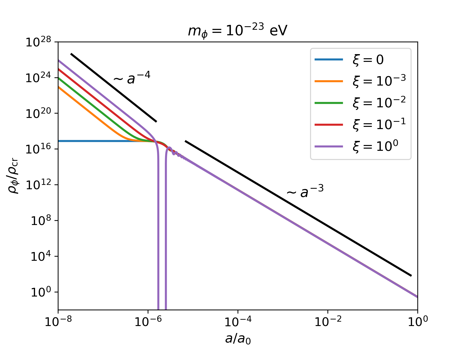
(a) Energy density as a function of scale factor for different values of $\xi$.

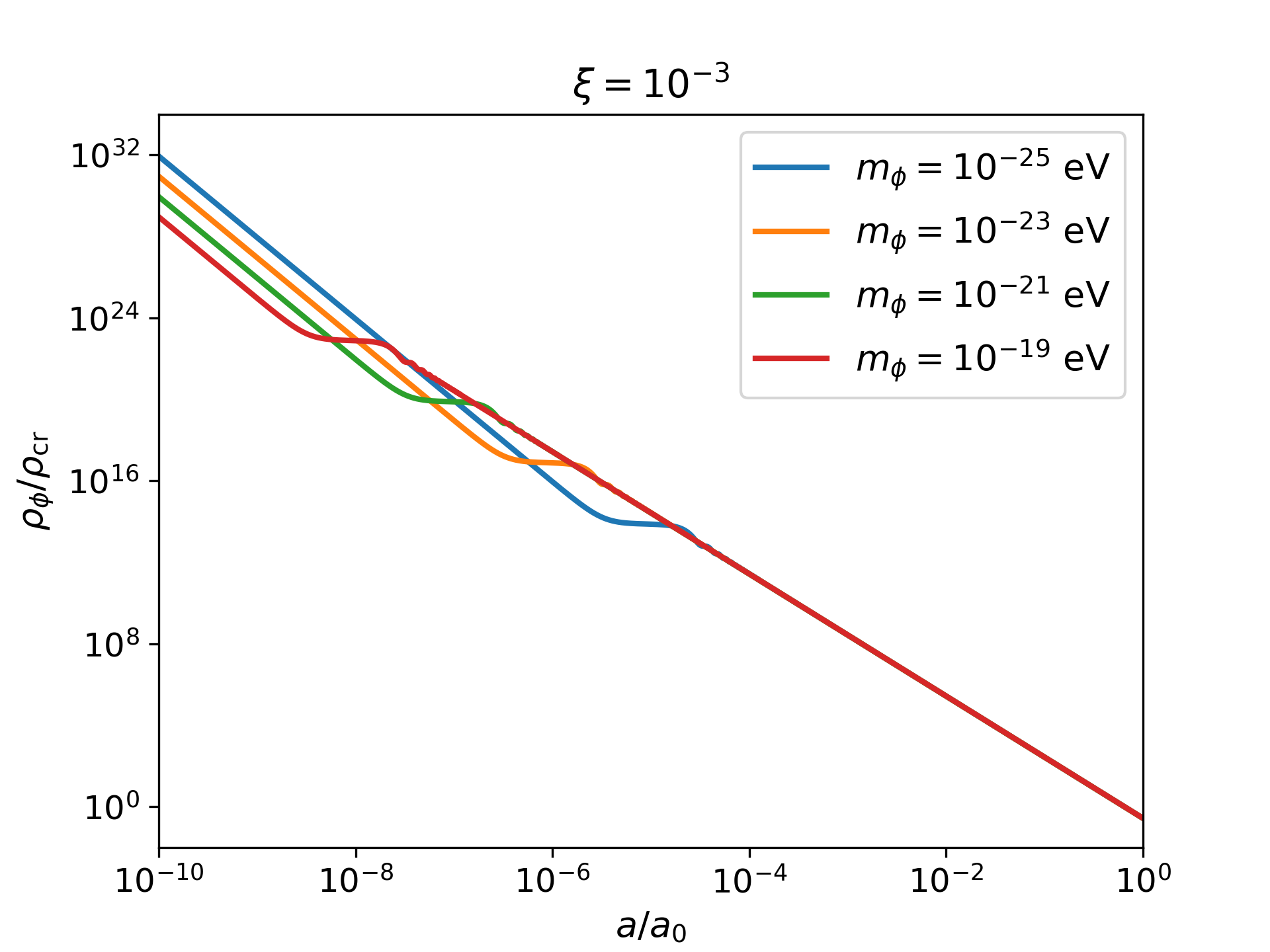
(b) Energy density as a function of scale factor for different values of $m_{\phi}$.

Figure 1: Evolution of ULA energy density displayed in terms of the critical density at the current epoch: $\rho_{\rm cr}=3H^{2}(t_{0})/8\pi G$

Figures 1(a) and 1(b) display the evolution of the energy density of the scalar field for different values of $\xi$ and scalar-field masses. First, we briefly summarize the well-known behavior for a minimally coupled field. During the initial phase, $y\ll 1$ and $\theta\ll 1$ (see Appendix B.1 for details). During this phase, the friction term [the term proportional to $\dot{\phi}_{0}$ in Eq. (5)] dominates. This causes the scalar-field energy density [Eq. (7)] to be nearly constant, resulting in the scalar field behaving as a cosmological constant. For $m_{\phi}\gtrsim H$, the scalar field starts oscillating around $\phi_{0}=0$. This phase culminates with the oscillation frequency converging to $\simeq m_{\phi}t$. For $m_{\phi}t\gg 1$, the rate of this oscillation far exceeds the expansion timescale, and as our aim is to track the evolution of relevant quantities on the expansion timescale, we define time-averaged quantities where the time average is over rapid oscillations. During this phase, the time-averaged $\phi_{0}$ vanishes and the time-averaged scalar-field energy density falls as $a^{-3}$ or it behaves as nonrelativistic matter as cold dark matter. For numerical stability, we employ the WKB approximation during the oscillatory phase and switch from the oscillatory solutions to the time-averaged evolution at $\theta=\pi/2$ (for further details see e.g. [54]).

Figure 1(a) shows that for nonzero $\xi$, the scalar-field energy density scales as $a^{-4}$ during the initial phase like the energy density of relativistic components (photons and neutrinos). In the intermediate phase, for $\xi\lesssim 10^{-1}$, the scalar field makes a transition to a phase in which its energy density is constant. For $\xi\gtrsim 1$, the energy density in the intermediate phase can become negative. At a later stage, $a\simeq 10^{-6}$, the energy density starts falling off as $a^{-3}$ for all values of $\xi$ for $m_{\phi}=10^{-23}$ eV. Figure 1(b) shows the impact of changing $m_{\phi}$ for a fixed $\xi$ on the energy density. For larger $m_{\phi}$, the field enters both the constant energy density phase and the $a^{-3}$ phase earlier.

In this paper, we focus on the range of values of $\xi$ for which the scalar-field energy density is always a positive quantity. Thus, we work with $\xi\lesssim 1$.

In Fig. 2, we further investigate the relative contribution of different terms in the equation of motion of nonminimally coupled scalar fields (Eq. (5)). It is seen that the term proportional to the nonminimal coupling $\xi$ always dominates at initial times. This term is $\propto H^{2}$ and follows from the corresponding term in the scalar-field Lagrangian, Eq. (2), which is proportional to the Ricci scalar $R\propto H^{2}$. This causes the energy density of the scalar field to behave as radiation during early times. At later times, the nonminimal coupling term becomes smaller than other terms, mainly owing to the rapid decrease in $H^{2}$, and the nonminimally coupled model behaves as a minimally coupled model.

This shows that the main difference in the background evolution between the minimally and nonminimally coupled scalar fields is during the initial phase: The energy density of the minimally coupled scalar field ($\xi=0$) is constant during this phase while it falls as $a^{-4}$ for nonzero $\xi$.

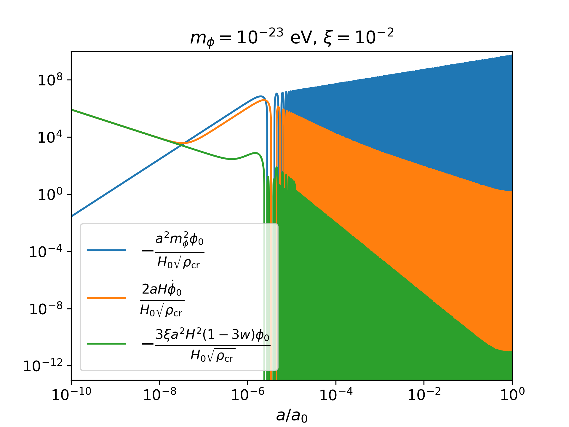
Figure 2: Different terms of Eq. (5) shown as a function of time.

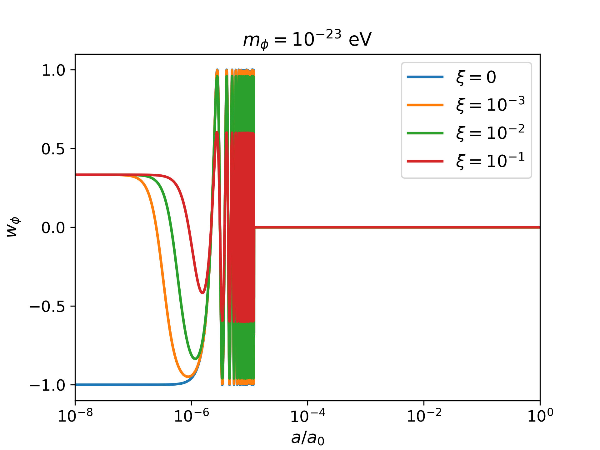
Figure 3: Evolution of the scalar-field equation of state $w_{\phi}$ displayed for different values of $\xi$. The plot is exact for $a\lesssim 10^{-5}$. For $a\gtrsim 10^{-5}$, the time average of $w_{\phi}$ is shown (see text for more details).

The evolution of the scalar-field equation of state $w_{\phi}$ is shown in Fig. 3. In the figure, we switch from the full solution to the time-averaged solution at $a=10^{-5}$. We tried to show the oscillations in $w_{\phi}$; for the actual solution, we switch to the time-averaged solution at $\theta=\pi/2$, as discussed above. As follows from the discussion above, the minimally coupled scalar field starts as a cosmological constant with $w_{\phi}=-1$ while the nonminimally coupled scalar field has the equation of state, $w_{\phi}=1/3$ (or it mimics radiation) during the initial phase, irrespective of the value of $\xi$. This radiationlike behaviour of a nonminimally coupled scalar field at early times can also be inferred from Eq. (13). At early times, $y\ll 1$ and $\theta\ll 1$ (Appendix B.1). Further, using the fact that $\Omega_{\gamma}$ and $\Omega_{\nu}$ dominate other density parameters during the radiation-dominated era, $w_{\phi}$ becomes

$$w_{\phi}\simeq\frac{8\frac{\xi}{y^{2}}(1-6\xi)+48\frac{\xi^{2}}{y^{2}}}{24\frac{\xi}{y^{2}}}=\frac{1}{3}.$$ (23)

During intermediate times, the equation of state $w_{\phi}$ tends to $-1$ for the nonminimally coupled case also. For $m_{\phi}\gtrsim H$, $w_{\phi}$ oscillates between positive and negative values, averaging to zero, for all the cases.

III.2 First order solution

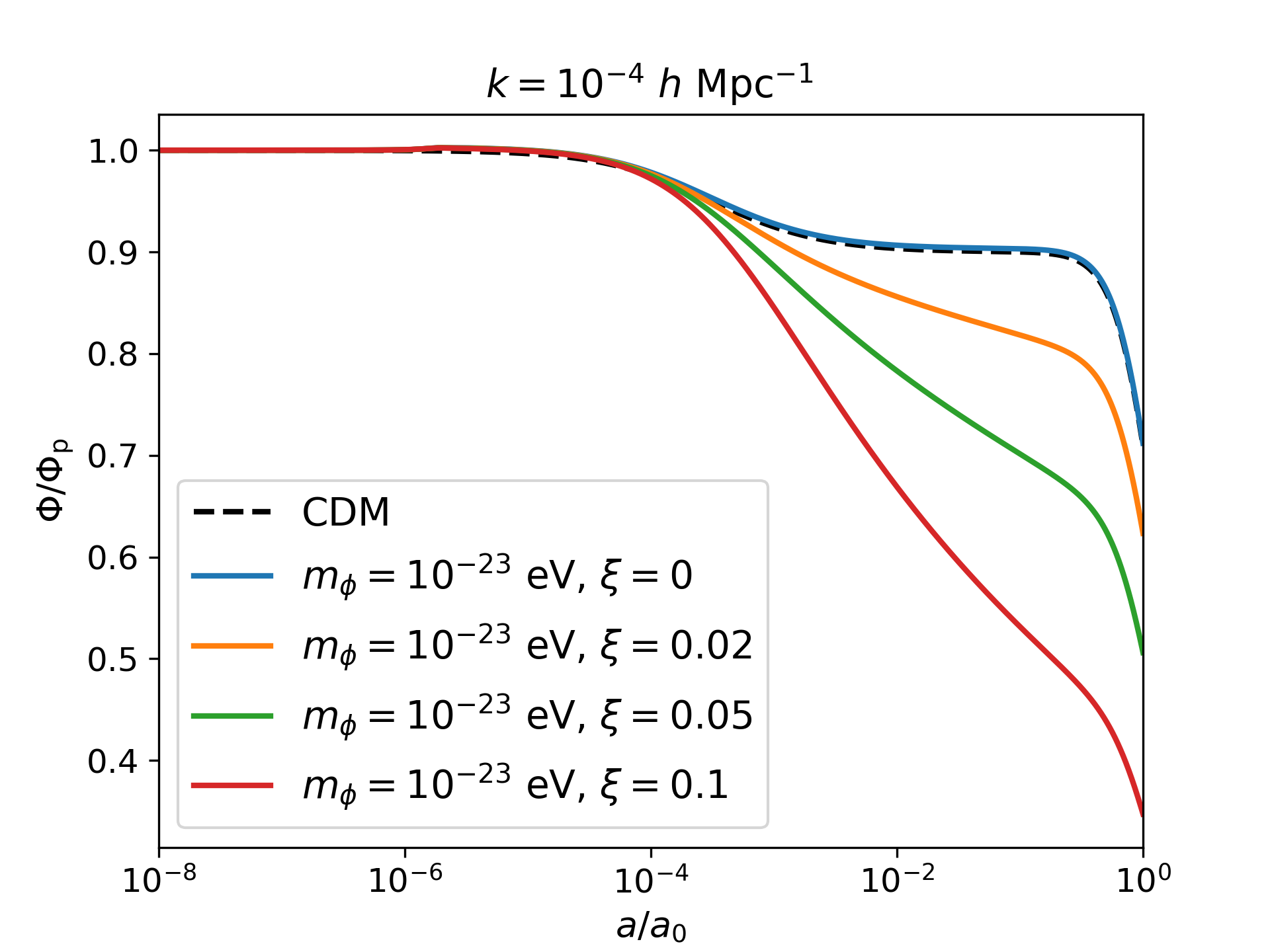
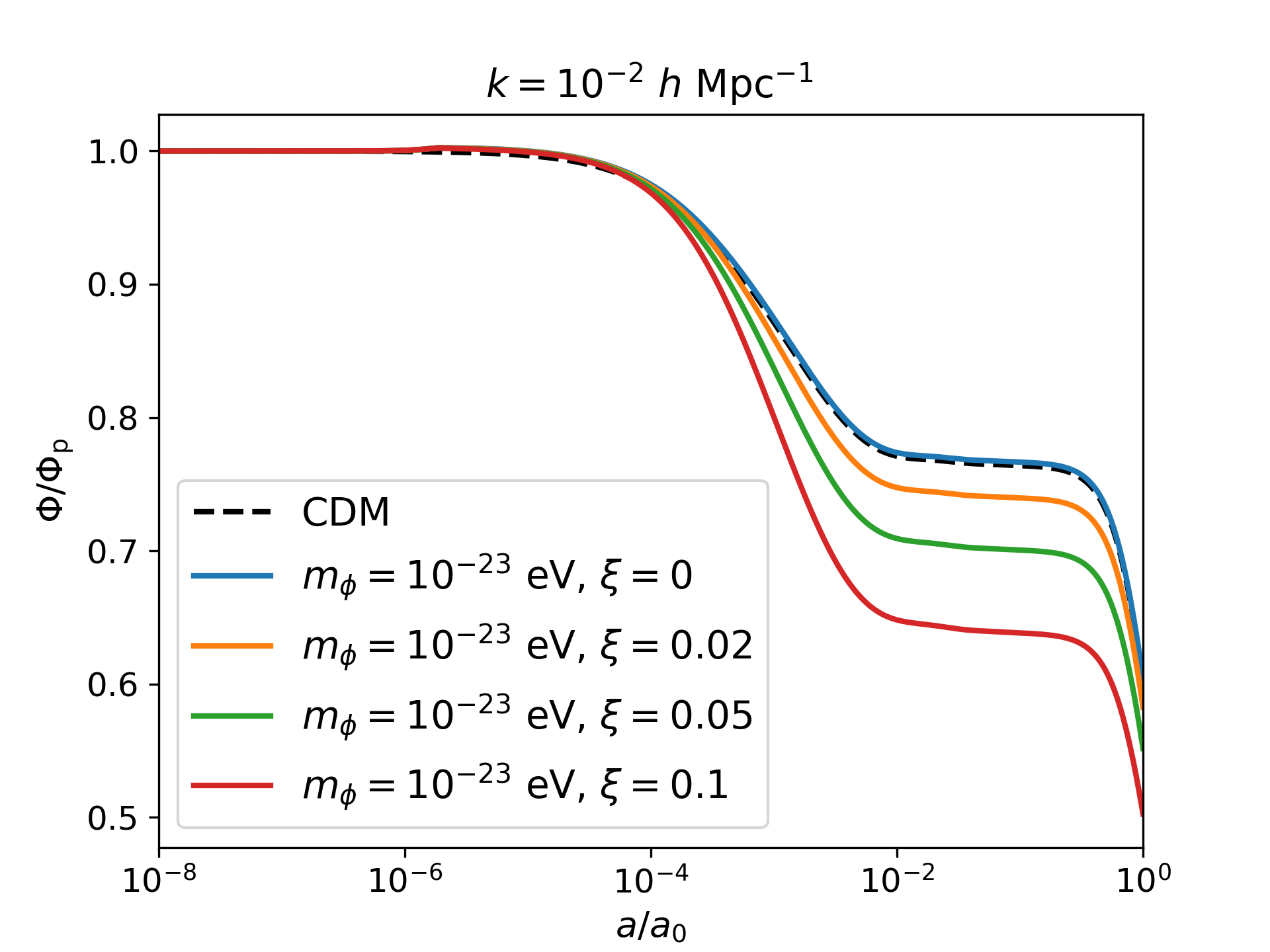
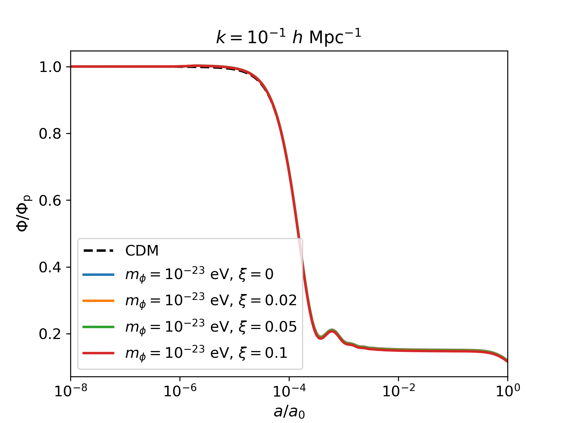
Figure 4: Scalar metric perturbation $\Phi$ (adiabatic mode) shown as a function of the scale factor for different values of $k$. Note that $\Phi_{p}$ is the primordial value of $\Phi$.

To gauge the impact of nonminimal coupling, we show the evolution of the metric perturbation $\Phi$ and the scalar-field density perturbation $\delta_{\phi}$ for the adiabatic mode for $k=10^{-4}\ h$ Mpc^-1, $10^{-2}\ h$ Mpc^-1, and $10^{-1}\ h$ Mpc^-1 in Figs. 4 and 5, respectively. We show four different $\xi$ values with $m_{\phi}=10^{-23}$ eV. We also plot the evolution of $\Phi$ and $\delta_{\rm{CDM}}$ in the usual $\Lambda$CDM case for reference.

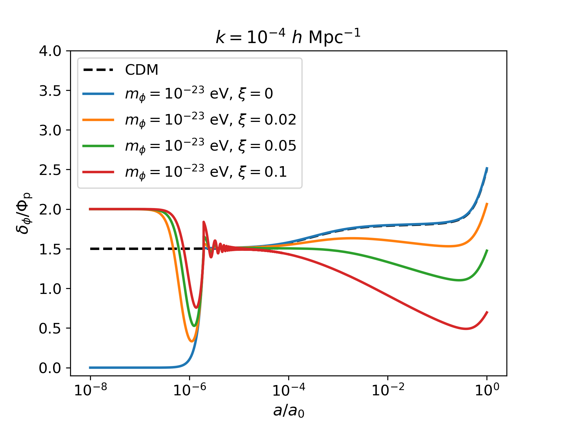
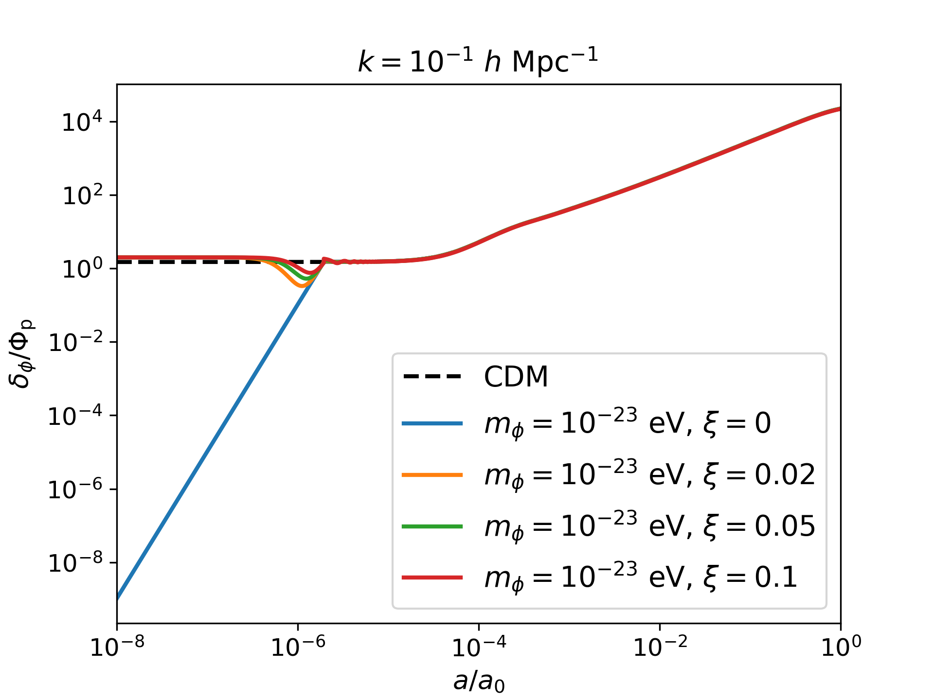
Figure 5: Evolution of ULA density perturbation $\delta_{\phi}$ (adiabatic mode) displayed for different values of $k$. Note that $\Phi_{p}$ is the primordial value of the metric perturbation $\Phi$.

We first summarize the features seen in Figs. 4 and 5: (a) The evolution of $\Phi$ for a minimally coupled scalar field ($\xi=0$) agrees with the CDM case for all values of $k$. (b) After the matter-radiation equality, the density perturbations for the minimally coupled scalar field coincide with the CDM model. (c) For the nonminimally coupled case, both $\Phi$ and $\delta_{\phi}$ are suppressed after the matter-radiation equality for small $k$. The suppression is seen to scale with $\xi$ for a given $k$. The impact of the nonminimal coupling decreases for smaller scales for a fixed $\xi$. The scales that enter the horizon before the matter-radiation equality ($k\geq 10^{-1}\ h$ Mpc^-1) are not affected appreciably by the nonminimal coupling. (d) For a minimally coupled scalar field, the initial density perturbation $\delta_{\phi}$ is zero, whereas for the nonminimally coupled case, it has an initial value of $2\Phi_{\rm p}$, the same initial condition as for $\delta_{\gamma}$, the photon density perturbation (for further details see Appendix B). Thus, even at first order, a nonminimally coupled scalar field behaves like radiation at early times.

The main impact of nonminimal coupling is on large scales, in particular scales that enter the horizon at late times. We focus on this issue below.

To understand Figs. 4 and 5, we first consider the evolution of the potential, $\Phi$, for the $\Lambda$CDM model. In the $\Lambda$CDM model, the potential drops by a factor of 9/10 after matter-radiation equality for scales that enter the horizon deep in the matter-dominated era ($k=10^{-4}\ h\ \rm Mpc^{-1}$ in Fig. 4), while the decay is larger for smaller scales (e.g. [76, 17]). The potential decays again when the universe becomes dominated by the cosmological constant at $z\lesssim 0.7$.

The decay of $\Phi$ by a factor of 9/10 for the long wavelength modes can be understood within the framework of multicomponent fluids in the $\Lambda$CDM model. In the $\Lambda$CDM model, both the background and the first order perturbations (on superhorizon scales) are dominated by relativistic components, photons and neutrinos, in the radiation-dominated era with an effective equation of state $w\simeq 1/3$ [Eq. (6)] and an adiabatic sound velocity $c_{s}^{2}\equiv\delta p/\delta\rho\simeq 1/3$. In the matter-dominated era, cold dark matter dominates the dynamics and both $w$ and $c_{s}^{2}$ vanish. In addition, the initial conditions for all components are assumed to be adiabatic, which implies that the pressure perturbations are entirely specified by density perturbations: $\delta p=c_{s}^{2}\delta\rho$. Under these conditions, it can be shown analytically that the initial potential at large scales falls by a factor of 9/10 after the matter-radiation equality (for details, see [76]).

In the ULA model, the background evolution of the scalar field behaves as a pressureless fluid, $\langle w\rangle=0$, for $z\lesssim 10^{5}$ (Fig. 3). However, many of the other conditions satisfied by the $\Lambda$CDM model do not hold for this model. In particular, the behavior of pressure perturbations is more complicated in this case (Eq. (21)). While the pressure perturbations become negligible for small scales for $z\lesssim 10^{5}$, they could be significant for large scales even after the matter-radiation equality. In addition, for ULA models, it is not possible to express pressure perturbations entirely in terms of density perturbations [Eqs. (19) and (21)]. This means the pressure perturbations in the scalar field are not purely “adiabatic” and the “entropy” part of the perturbation provides an additional source of perturbations. An important distinction between the minimal and nonminimal coupling is that for the minimal coupling this split renders both $c_{s}^{2}$ and entropy perturbations singular. However, for the nonminimally coupled case, the split is well behaved (for detailed discussion, see [73]).

These additional features of the ULA model could cause the potential to behave differently from the usual case. For a minimally coupled case, the impact of these additional features is negligible and we notice that the behavior of $\Phi$ is similar to the CDM case. However, for the nonminimally coupled case, pressure perturbations of the scalar field could play an important role during the transition from radiation to matter domination and cause the potential to decay for a longer period extending into the matter domination. As the pressure perturbations are related to other perturbations through energy-momentum conservation conditions, we expect a significant impact on other components of matter perturbations also. In particular, Fig. 5 shows that the density contrast for the scalar field also decays for $k\simeq 10^{-4}h\,\rm Mpc^{-1}$. This anomalous behavior of density perturbations for large scales results in a significant change in the observable matter power spectrum.

From density contrasts of different components, we can compute the matter power spectrum $P(k,t_{0})$ (e.g. [17]):

$$P(k,t_{0})=\frac{A}{k^{3}}\bigg{(}\frac{k}{H_{0}}\bigg{)}^{n-1}\Omega_{m}^{2}\delta_{\rm net}^{2}(k,t_{0}).$$ (24)

Here $\delta_{\rm net}=\sum_{i}f_{i}\delta_{i}$ with $f_{i}\equiv\Omega_{i}/\sum_{i}\Omega_{i}$ and $\delta_{i}$ being the fraction and density contrast of different components. At the current epoch, only the scalar field and baryons provide important contributions to the density contrast, and we use values of $f_{i}$ given by the best-fit Planck parameters for baryons and CDM. Here $\Omega_{m}=\Omega_{\phi}(t_{0})+\Omega_{b}(t_{0})$ is the value of the total matter density parameter at the current epoch, $A$ is a constant whose value is determined by matching the theoretical matter power spectrum to cosmological observables, and $n$ is the scalar spectral index of the initial matter power spectrum generated during the inflationary era: $P(k,t_{i})\propto k^{n}$ with $n\simeq 1$. In this paper, we use the best-fit value obtained by the Planck Collaboration, $n=0.96$ [13].

The matter power spectrum is probed by the Planck CMB data for scales in the range $k\simeq 10^{-4}\hbox{--}10^{-1}h\,\rm Mpc^{-1}$ (e.g. [12]). Using Planck data, the matter power spectrum can be reconstructed in the aforementioned range [77]. The SDSS galaxy clustering data measure the power spectrum for $k\simeq 10^{-2}\hbox{--}0.4h\,\rm Mpc^{-1}$ [2]. We note that only the galaxy data for $k\lesssim 0.1\,\rm Mpc^{-1}$ can be directly compared with the prediction of linear perturbation theory, as linear theory fails for smaller scales at the current epoch (e.g. [17]). The CMB and galaxy clustering data are compatible with each other using the results of general relativistic perturbation theory for the usual $\Lambda$CDM model (which includes the inflation-generated initial power-law matter power spectrum [see the discussion following Eq. (24), e.g. [12]]). One can normalize the matter power spectrum using Planck CMB temperature anisotropy and CMB lensing measurements (e.g. [77]). Alternatively, it can be normalized using the abundance of low-redshift massive clusters and cosmological weak lensing data at $z\lesssim 1$ (e.g. [17] and references therein). These data can be used to construct $\sigma_{8}$, the mass dispersion at the scale $8h^{-1}\rm Mpc$. Planck results give $\sigma_{8}=0.81$ [12], which is in agreement with the low redshift data.

In Fig. 6, we show the matter power spectra for $\xi=0$. Both the adiabatic and isocurvature modes are shown for a fixed ULA mass, $m_{\phi}=10^{-23}$ eV. The matter power for the two modes is matched at large scales to the $\Lambda$CDM model. For the range of scales shown in Fig. 6, $k\lesssim 0.3h\,\rm Mpc^{-1}$, the matter power spectrum for the minimally coupled scalar field agrees with the power spectrum for the usual $\Lambda$CDM case. This inference is compatible with existing results in the literature (e.g. [54]). We note that, for the case shown in Fig. 6, the ULA matter power spectrum has a power deficit as compared to the $\Lambda$CDM model at smaller scales, $k\gtrsim 1$ Mpc^-1 (these scales are not shown in the figure), and multiple studies have considered the implications of this small-scale matter power suppression [49, 50, 51, 52, 56, 57, 61, 62, 63, 55, 64]. However, our focus in this paper is on large scales.

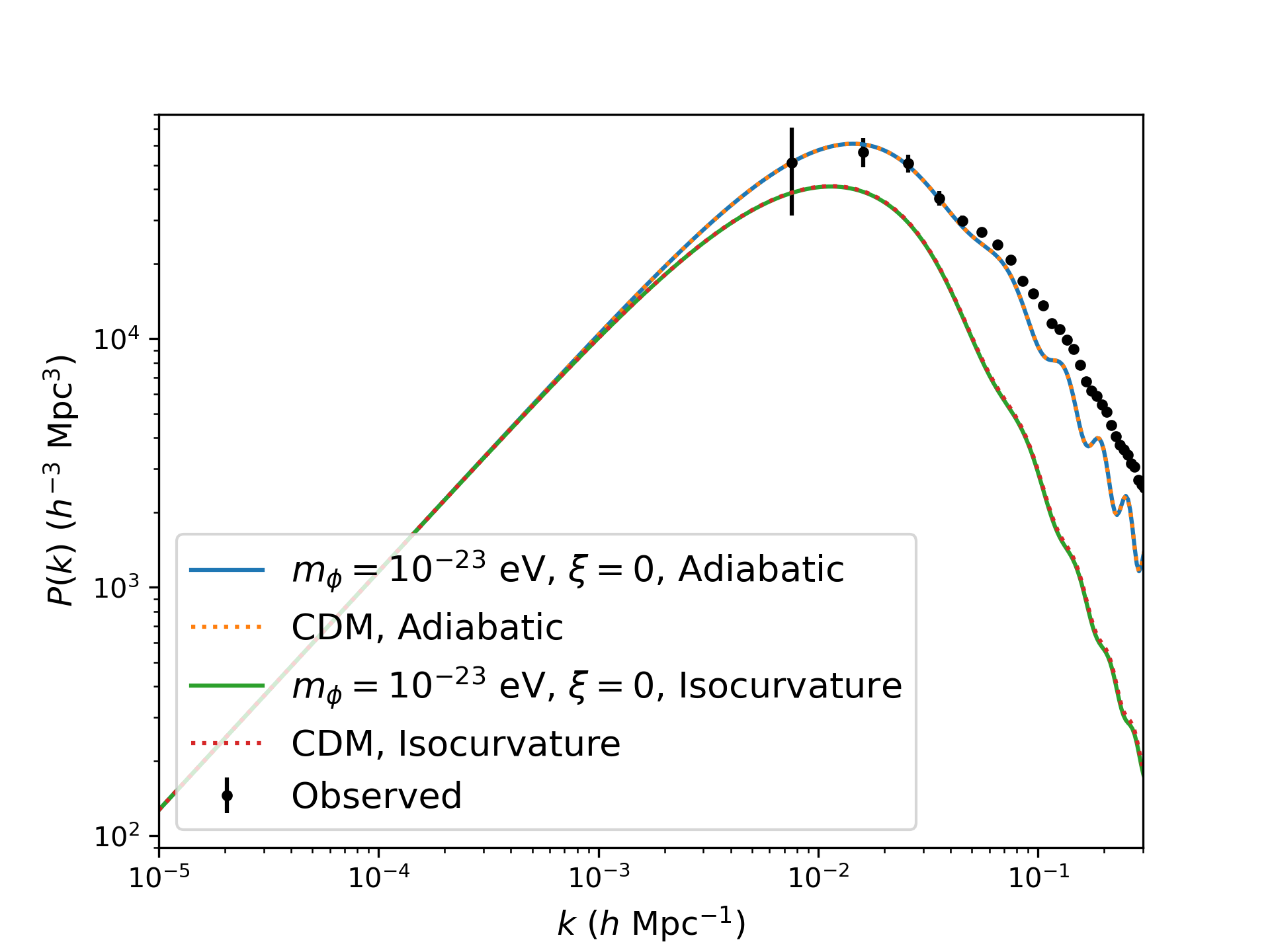
Figure 6: Adiabatic and isocurvature matter power spectra shown for minimally coupled axions for $m_{\phi}=10^{-23}$ eV. The $\Lambda$CDM model results are also shown for comparison. The data points corresponding to the monopole of the measured galaxy power spectrum from SDSS are also shown (e.g. [78]).

In Fig. 7, we display the matter power spectrum for the nonminimally coupled case for $m_{\phi}=10^{-23}$ eV. As discussed above, in this case, the density perturbations in the scalar field deviate from the CDM density perturbations at large scales but reproduce the results of the CDM model at small scales. This leaves observable traces on the observed matter power spectrum. We match the matter power spectrum to the $\Lambda$CDM model at large scales. Given the decay of density perturbations on large scales for the nonminimally coupled scalar field (Fig. 5), the matter power is expected to differ between the nonminimal coupling case and the $\Lambda$CDM (or minimal coupling case) at small scales. As a result, the matter power is found to be significantly larger at small scales as compared to the CDM power spectrum. Alternatively, if we had chosen to normalize the power spectrum at small scales (e.g. by choosing the measured value of $\sigma_{8}$ by cluster abundance data), we would find a deficit of matter power at large scales. The power excess in Fig. 7 is proportional to the value of $\xi$. To obtain agreement with both the large- and small-scale data, we obtain the following constraint on the nonminimal coupling for the adiabatic mode: $\xi\lesssim 0.01$.

Figure 7 also shows that, for nonminimal coupling, the matter power spectrum for the isocurvature mode is in much better agreement with the usual adiabatic CDM mode. For instance, the isocurvature mode for $\xi=0.05$ agrees well with the $\xi=0$ adiabatic mode at large scales. We do not carry out a more detailed comparison here but our results suggest that a mix of adiabatic and isocurvature initial conditions for the nonminimally coupled ULAs might behave similarly to the CDM adiabatic mode.

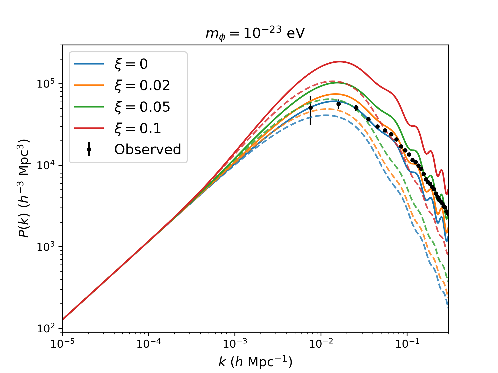
Figure 7: Adiabatic and isocurvature matter power spectra for the nonminimally coupled ULAs shown for different values of $\xi$. The solid lines denote the adiabatic power spectra and the dashed lines show the isocurvature power spectra.

In Figs. 4, 5, and 7, we show results for a fixed ULA mass $m_{\phi}=10^{-23}\,\rm eV$ as a function of the nonminimal coupling. For our work we consider a mass range $10^{-25}\,{\rm eV}<m_{\phi}<10^{-19}\,\rm eV$. We note that the large-scale behavior shown in the figures is obtained for this entire range of masses. The best reported upper limit on the mass $m_{\phi}\gtrsim 10^{-20}\,\rm eV$ arises from the small-scale behavior of the power spectrum using the Lyman-$\alpha$ data [64]. Our main results are compatible with this upper limit.

IV Conclusion

In this paper, we study a nonminimally coupled scalar-field as a potential cold dark matter candidate. The minimal scalar field models have been extensively studied as ultralight axions in the literature and are known to alleviate well-known small-scale issues with the usual $\Lambda$CDM model. Our study is a natural extension of such models.

The dynamics of both the background and the perturbed components of the scalar field change substantially for the nonminimally coupled case. Initially, the background scalar field behaves as radiation, unlike the usual case in which the scalar-field energy starts as a cosmological constant. For a scale factor in the range $a\simeq 10^{-5}\hbox{--}10^{-7}$, the nonminimally coupled scalar field makes a transition to the cosmological-constant domination phase (Fig. 1). The altered initial evolution yields a new constraint on such models from primordial nucleosynthesis. During primordial nucleosynthesis, the final abundance of helium-4 and deuterium is a sensitive function of the total radiation content of the universe at $a\simeq 10^{-9}$. A comparison of current data with the theory of formation of light elements suggest that the amount of “dark radiation” could not exceed 10% of the radiation energy density given by photons and the standard model neutrinos during that era (e.g. see [79] and references therein). This constrains the strength of the gravity-scalar-field coupling $\xi\lesssim 10$ for the range of scalar-field masses we consider here.

The first order perturbation theory of a nonminimally coupled scalar field adds multiple new complexities as compared to the usual case. One of the new features is the presence of anisotropic stress, which mainly impacts small scales [Eq. (22)]. Our most important finding in this paper relates to large scales. For nonzero $\xi$, the perturbations on scales that enter the horizon after the matter-radiation equality could have radically different behavior (Figs. 4 and 5). This causes the matter power spectrum to deviate significantly from the minimal coupling case (Fig. 7). For adiabatic initial conditions, a comparison of the computed matter power spectrum with galaxy clustering and CMB anisotropy data puts strong constraints on the nonminimal coupling: $\xi\lesssim 0.01$.

We also consider isocurvature initial conditions. More specifically, we consider the scalar-field isocurvature mode in which only the scalar-field density contrast is nonzero initially. Figure 7 shows that this isocurvature mode for nonzero $\xi$ agrees with the adiabatic CDM (or minimally coupled) mode at large scales. This means that a mix of isocurvature and adiabatic initial conditions might explain the observed matter power spectrum for a nonminimally coupled ULA.

In the current work, we focus on computing the matter power spectrum for nonminimally coupled ULAs and compare the prediction of the model with the galaxy power spectrum and CMB results. This yields an approximate bound on the strength of nonminimal coupling. A more detailed multiparameter analysis based on either the Fisher matrix or MCMC methods will give more precise constraints. This work also needs to be extended to CMB temperature and polarization anisotropies, as a direct comparison with the CMB anisotropy data would help quantify our results further. In particular, the new physics our model introduces might result in novel outcomes such as the following: (a) the integrated Sachs-Wolfe effect would be altered owing to the time dependence of the potential at large scales, (b) the sound horizon close to the era of recombination might change such that it would have a bearing on the issue of Hubble tension between the CMB and low-redshift data (e.g. [80] and references therein). We hope to return to these issues with the theoretical computation of the CMB temperature and polarization anisotropies and a more detailed statistical comparison with cosmological data in a future work.

V Acknowledgement

We thank Dr. Florian Beutler for providing us with the data points for the observed galaxy power spectrum.

Appendix A EINSTEIN AND FLUID EQUATIONS

In this section, we give the necessary cosmological equations, including Einstein equations and the relevant equations for photons, baryons, neutrinos, and cosmological constant at zeroth and first order (for details, see e.g. [74, 73, 75, 17, 54]).

A.1 Background equations

For the sake of completeness and consistency of notations, we list the relevant equations for the background evolution of the universe.

We have already defined the scalar field, photon, and neutrino density parameters in Sec. II.1. We can similarly define the density parameter for any component of the universe by

$$\Omega_{i}=\frac{8\pi G\rho_{i}}{3H^{2}}.$$ (25)

We denote the baryon density parameter by $\Omega_{b}$ and the cosmological-constant density parameter by $\Omega_{\Lambda}$.

In general, the density parameter for the $i$th component evolves as

$$\Omega_{i}^{\prime}=3(w-w_{i})\Omega_{i},$$ (26)

where $w_{i}$ is the equation of state of the $i$th component. Thus, the density parameters evolve according to the following equations:

$$\Omega_{\gamma}^{\prime}=3\bigg{(}w-\frac{1}{3}\bigg{)}\Omega_{\gamma},$$ (27)

$$\Omega_{\nu}^{\prime}=3\bigg{(}w-\frac{1}{3}\bigg{)}\Omega_{\nu},$$ (28)

$$\Omega_{b}^{\prime}=3w\Omega_{b},$$ (29)

$$\Omega_{\Lambda}^{\prime}=3(w+1)\Omega_{\Lambda}.$$ (30)

Using Eq. (6), these equations specify the evolution of all the density parameters. In addition to these fluid equations, we have two Einstein equations given by

$$H^{2}=\frac{\dot{a}^{2}}{a^{4}}=\frac{8\pi G}{3}\sum_{i}\rho_{i},$$ (31)

$$\dot{H}=-4\pi Ga\sum_{i}(\rho_{i}+p_{i}).$$ (32)

Equation (31) can be written in terms of the density parameters as

$$\Omega_{\gamma}+\Omega_{\nu}+\Omega_{\phi}+\Omega_{b}+\Omega_{\Lambda}=1.$$ (33)

On the other hand, Eq. (32) converts to an equation for $y$, defined in Sec. II.1 as $y=2m_{\phi}/H$. We obtain

$$y^{\prime}=\frac{3}{2}(1+w)y.$$ (34)

Equations (10)–(13), along with Eqs. (27)–(30) and (33)–(34), constitute the complete set of background equations.

A.2 First order equations

In Fourier space, the first order equations for photons, neutrinos, and baryons are (for details, see e.g. [74, 73, 75, 17])

$$\Theta_{0}^{\prime}+\frac{k}{aH}\Theta_{1}=-\Phi^{\prime},$$ (35)

$$\Theta_{1}^{\prime}-\frac{k}{3aH}\Theta_{0}=\frac{k}{3aH}\Psi-\frac{n_{e}\sigma_{T}}{H}\bigg{(}\Theta_{1}-\frac{iv_{b}}{3}\bigg{)},$$ (36)

$$\mathcal{N}_{0}^{\prime}+\frac{k}{aH}\mathcal{N}_{1}=-\Phi^{\prime},$$ (37)

$$\mathcal{N}_{1}^{\prime}-\frac{k}{3aH}\left(\mathcal{N}_{0}-\mathcal{N}_{2}\right)=\frac{k}{3aH}\Psi,$$ (38)

$$\delta_{b}^{\prime}+\frac{ik}{aH}v_{b}=-3\Phi^{\prime},$$ (39)

$$v_{b}^{\prime}+v_{b}=-\frac{ik}{aH}\Psi-\frac{n_{e}\sigma_{T}}{HR}(v_{b}+3i\Theta_{1}).$$ (40)

Our notation is consistent with that of Dodelson [17]. Here $\Theta_{0}$ and $\Theta_{1}$ are the monopole and the dipole components of the photon temperature perturbation, respectively; $\mathcal{N}_{0}$ and $\mathcal{N}_{1}$ are the monopole and dipole components of the neutrino temperature perturbation, and $\mathcal{N}_{2}$ is the quadrupole moment. The quadrupole moment for photons is omitted as it is negligible in the tight-coupling approximation [17]. Note that $\delta_{b}=\delta\rho_{b}/\rho_{b}$ is the baryon overdensity, $v_{b}$ is the bulk velocity of baryons, $n_{e}$ is the electron number density, $\sigma_{T}$ is the Thomson scattering cross section, and $R=3\Omega_{b}/4\Omega_{\gamma}$ is the baryon-energy-to-photon-energy ratio.

We simplify photon equations further in the tight-coupling approximation and retain terms up to the first order in the scattering timescale, $1/(n_{e}\sigma_{T}c)$. This procedure neglects Silk damping, which is needed for accurate treatment of CMB anisotropies and the matter power spectrum at small scales. However, it makes a negligible impact on our treatment as the main impact of our results is at large scales. For massless neutrinos, we adopt $\mathcal{N}_{2}=0$ and neglect higher multipoles. These modes play an important role for subhorizon modes, $k\eta>1$. For $\ell\geq 2$, these modes decay as $j_{\ell}(k\eta)$ after the horizon entry (e.g. Ma and Bertschinger [75]). We check the efficacy of our procedure by putting neutrino perturbation to zero after the horizon entry, and we find that a more precise treatment of higher neutrino multipoles does not significantly affect the predicted matter power spectrum on the scales of interest to us.

The perturbed metric components, $\Phi$ and $\Psi$, obey the following first order Einstein equations.

$$\Phi^{\prime}-\Psi+\frac{k^{2}}{3a^{2}H^{2}}\Phi=\frac{1}{2}(4\Omega_{\gamma}\Theta_{0}+4\Omega_{\nu}\mathcal{N}_{0}\\ +\Omega_{\phi}\delta_{\phi}+\Omega_{b}\delta_{b}),$$ (41)

$$\Phi^{\prime}-\Psi=-\frac{3}{2}\frac{aH}{k}[4\Omega_{\gamma}\Theta_{1}+4\Omega_{\nu}\mathcal{N}_{1}\\ +\Omega_{\phi}(1+w_{\phi})v_{\phi}+\Omega_{b}v_{b}],$$ (42)

$$\Phi^{\prime\prime}+3\Phi^{\prime}-\Psi^{\prime}-3\Psi-\frac{3}{2}(1+w)(\Phi^{\prime}-2\Psi)+\\ \frac{k^{2}}{3a^{2}H^{2}}(\Phi+\Psi)=-\frac{3}{2}\bigg{(}\frac{4}{3}\Omega_{\gamma}\Theta_{0}+\frac{4}{3}\Omega_{\nu}\mathcal{N}_{0}+\Omega_{\phi}w_{\phi}\pi_{\phi}\bigg{)},$$ (43)

$$-\frac{k^{2}}{3a^{2}H^{2}}(\Phi+\Psi)=\Omega_{\phi}w_{\phi}\Pi_{\phi}.$$ (44)

Equations (17)–(22), along with Eqs. (35)–(44), constitute the complete set of first order equations. Not all of these first order equations are independent of each other. In particular, we solve two Einstein’s equations [Eqs. (41) and (44)] along with the fluid equations. The other two Einstein’s equations can be derived from the equations we use (for details, see e.g. Kodama and Sasaki [73]).

Appendix B INITIAL CONDITIONS

To obtain the initial conditions, we analytically solve the set of background and first order equations in the radiation-dominated era such that $k\eta\ll 1$ for all scales of interest to us. However, for nonminimally coupled scalar fields, the complex nature of equations does not always permit an analytic solution even at early times. In such cases, we choose the initial condition for $\xi=0$ and numerically search for the suitable initial conditions for the nonminimally coupled case. We assume that the correct solution is an attractor solution and the approximate initial conditions allow us to reach the relevant solution once the nonminimally coupled field enters the cosmological-constant-dominated phase.

We follow the work of Ureña-López and Gonzalez-Morales [54] to obtain the initial conditions for variables related to ULAs. For initial conditions for other variables, we follow the work of Dodelson [17].

B.1 Background initial conditions

We find the initial conditions at the scale factor $a=a_{i}$ such that $m_{\phi}/H_{i}\ll 1$, that is, $y_{i}\ll 1$. This is expected deep in the radiation-dominated epoch. Thus, we expect $\Omega_{\gamma i}+\Omega_{\nu i}\simeq 1$, and $\Omega_{ai}\ll 1$ for $a\neq\gamma,\ \nu$. The initial condition for the scalar field is chosen such that $\dot{\phi}_{i}=0$ and $\phi_{i}<0$. Therefore, the initial value of $\theta$ satisfies the condition: $\theta_{i}\ll 1$ [Eqs. (8) and (9)].

Using these approximations, we have, at early times, $H=H_{0}\sqrt{\Omega_{\gamma 0}+\Omega_{\nu 0}}/a^{2}$. Thus, we have the initial condition for $y$,

$$y_{i}=\frac{2m_{\phi}}{H_{i}}=\frac{2m_{\phi}a_{i}^{2}}{H_{0}\sqrt{\Omega_{\gamma 0}+\Omega_{\nu 0}}}.$$ (45)

Both Eqs. (10) and (11) contain a term $(1-3w)/y$. This term can be approximated at early times as follows.

$$1-3w =1-(\Omega_{\gamma}+\Omega_{\nu}+\Omega_{\phi})+3\Omega_{\Lambda}=\Omega_{b}+4\Omega_{\Lambda}.$$ (46)

Here, we have used Eq. (33) and the fact that, at early times, $w_{\phi}=1/3$ [see Eq. (23)]. From Eq. (25), we have $\Omega_{b}/(\Omega_{\gamma}+\Omega_{\nu})=\rho_{b}/(\rho_{\gamma}+\rho_{\nu})=a\rho_{b0}/(\rho_{\gamma 0}+\rho_{\nu 0})$. Thus, the initial condition for $\Omega_{b}$ is

$$\Omega_{bi}=\frac{\Omega_{b0}a_{i}}{\Omega_{\gamma 0}+\Omega_{\nu 0}}.$$ (47)

Similarly,

$$\Omega_{\Lambda i}=\frac{\Omega_{\Lambda 0}a_{i}^{4}}{\Omega_{\gamma 0}+\Omega_{\nu 0}}.$$ (48)

So, we obtain

$$\frac{1-3w}{y}=\frac{H_{0}}{2m_{\phi}\sqrt{\Omega_{\gamma 0}+\Omega_{\nu 0}}}\bigg{(}\frac{\Omega_{b0}}{a}+4\Omega_{\Lambda 0}a^{2}\bigg{)}$$ (49)

deep in the radiation-dominated epoch.

Finally, using the approximation $\theta_{i}\ll 1$, Eq. (11) gives

$$\theta^{\prime}=-3\theta+\frac{2m_{\phi}a^{2}}{H_{0}\sqrt{\Omega_{\gamma 0}+\Omega_{\nu 0}}}\\ +\frac{6\xi H_{0}}{m_{\phi}\sqrt{\Omega_{\gamma 0}+\Omega_{\nu 0}}}\bigg{(}\frac{\Omega_{b0}}{a}+4\Omega_{\Lambda 0}a^{2}\bigg{)}.$$ (50)

The solution to this ODE is

$$\theta=\frac{2}{5\sqrt{\Omega_{\gamma 0}+\Omega_{\nu 0}}}\bigg{(}\frac{m_{\phi}}{H_{0}}+\frac{12\xi H_{0}\Omega_{\Lambda 0}}{m_{\phi}}\bigg{)}a^{2}\\ +\frac{3\xi H_{0}\Omega_{b0}}{m_{\phi}\sqrt{\Omega_{\gamma 0}+\Omega_{\nu 0}}}\frac{1}{a}+\frac{C}{a^{3}},$$ (51)

where $C$ is the constant of integration. We neglect the fastest decaying mode, which is the last term in the solution. This gives the initial condition for $\theta$,

$$\theta_{i}=\frac{2}{5\sqrt{\Omega_{\gamma 0}+\Omega_{\nu 0}}}\bigg{(}\frac{m_{\phi}}{H_{0}}+\frac{12\xi H_{0}\Omega_{\Lambda 0}}{m_{\phi}}\bigg{)}a_{i}^{2}\\ +\frac{3\xi H_{0}\Omega_{b0}}{m_{\phi}\sqrt{\Omega_{\gamma 0}+\Omega_{\nu 0}}}\frac{1}{a_{i}}.$$ (52)

Obtaining the initial condition for $\widetilde{\Omega}_{\phi}$ in this manner is difficult. Thus, we put $\xi=0$ and follow the method used in the work of Ureña-López and Gonzalez-Morales [54]. This gives the following initial condition for $\widetilde{\Omega}_{\phi}$:

$$\widetilde{\Omega}_{\phi i}=K\frac{\Omega_{\phi 0}}{\Omega_{\gamma 0}+\Omega_{\nu 0}}a_{i}\bigg{[}\frac{4\theta_{i}^{2}}{\pi^{2}}\bigg{(}\frac{9+\pi^{2}/4}{9+\theta_{i}^{2}}\bigg{)}\bigg{]}^{3/4},$$ (53)

where $K$ is a constant that needs to be found numerically. We can use a binary search in order to find the value of $K$ which gives the correct value of $\Omega_{\phi 0}$, the present value of scalar-field density parameter. For the range of cases we consider for the nonminimally coupled ULAs, the value of $K$ can vary by many orders of magnitude.

The initial condition for $\Omega_{\nu}$ is given by

$$\Omega_{\nu i}=\frac{\Omega_{\nu 0}}{\Omega_{\gamma 0}+\Omega_{\nu 0}}.$$ (54)

B.2 First order initial conditions

For the first order equations, we consider two initial conditions: adiabatic and isocurvature. In a multicomponent fluid, these initial conditions can refer to different components. We adopt the usual adiabatic initial conditions in which the ratio of the number densities of different components is chosen to be the same (for a detailed discussion, see e.g. [75] or [76]). On the other hand, for isocurvature initial conditions, only the density perturbations associated with either the baryons or ULAs are nonzero initially. For instance, the ULA isocurvature mode has only $\delta_{\phi}\neq 0$ during very early times, while all other perturbation variables are set to zero. We consider only this isocurvature mode in our analysis.

Obtaining initial conditions at first order using analytic solutions for nonminimally coupled scalar fields is difficult. Therefore, as in the background case, we start our search for the suitable initial conditions with the $\xi=0$ case for both modes.

B.2.1 Adiabatic mode

Using Eqs. (22) and (44), we obtain $\Psi=-\Phi$ for $\xi=0$. For the adiabatic mode, the metric perturbation is constant deep in the radiation-dominated era. Therefore, $\Phi_{i}^{\prime}=0$. Further, we know from the previous section that as $a\to 0$, $y\to 0$ and $\theta\to 0$. Thus, at early times, from Eq. (18), we obtain

$$\lim_{a\to 0}\beta^{\prime}=-3\sin(\theta-\beta)-\frac{k^{2}}{k_{J}^{2}}[1-\cos(\theta-\beta)].$$ (55)

Note that $\theta=\beta$ is a critical point of the system. Substituting this value in Eq. (17), we obtain:

$$\alpha^{\prime}=-\frac{3}{2}\alpha(1+\cos\theta)+2y\cos\bigg{(}\frac{\theta}{2}\bigg{)}\Phi.$$ (56)

Considering $\theta$ to be negligible, we have

$$\alpha^{\prime}=-3\alpha+2y\Phi.$$ (57)

From Eqs. (45) and (52), we see that, at early times, $y=5\theta=5\theta_{i}(a/a_{i})^{2}$ for $\xi=0$. Substituting this value of $y$ in Eq. (57) and solving the resultant ODE, we obtain the following initial condition for $\alpha$:

$$\alpha_{i}=2\theta_{i}\Phi_{i}.$$ (58)

Here we have neglected a decaying mode.

Substituting the initial condition for $\alpha$ in Eq. (18), we get

$$\beta^{\prime}=-6\theta+3\beta+\frac{y}{\theta}(\theta-\beta)=-2\beta-\theta$$ (59)

for the $\xi=0$ case. Thus,

$$\beta^{\prime}=-2\beta-\theta_{i}\bigg{(}\frac{a}{a_{i}}\bigg{)}^{2}.$$ (60)

Solving this equation, and neglecting the decaying mode, we have

$$\beta_{i}=-\frac{\theta_{i}}{4}.$$ (61)

The initial conditions for other variables are given in the work of Dodelson [17]:

$$3\Theta_{0i}=3\mathcal{N}_{0i}=\delta_{bi}=\frac{3}{2}\Phi_{i},$$ (62)

$$3\Theta_{1i}=3\mathcal{N}_{1i}=iv_{bi}=-\frac{k}{2aH}\Phi_{i}.$$ (63)

Since $k/aH$ is negligible at very early times, $\Theta_{1i}=\mathcal{N}_{1i}=v_{bi}\approx 0$.

B.2.2 ULA isocurvature mode

For the ULA isocurvature case, we choose $\alpha_{i}=1$ and $\beta_{i}=-\pi$. This gives us $\delta_{\phi i}=1$ [see Eq. (19)]. All the other perturbation variables are set to zero initially, including the metric perturbations, $\Phi$ and $\Psi$.

Appendix C NUMERICAL IMPLEMENTATION

In this section, we briefly summarize the salient aspects of numerical implementation of the coupled Einstein-Boltzmann equations along with the scalar-field dynamics. We perform numerical integration of the relevant equations using PYTHON codes.

The background and first order initial conditions are set using the procedures described in Appendixes B.1 and B.2. We implement the initial conditions to the lowest order in $k\eta$ for the relevant variables, which means zeroth order for potentials and the density field, first order for bulk velocities, and second order for the anisotropic stress (for details, see e.g. [75]). Using matrix methods, one can systematically develop initial conditions to higher orders in $k\eta$ [81, 82, 83, 84, 55], which is harder for us to implement as the initial conditions for the ULA have to be determined numerically in our case.

We verify the robustness of our initial conditions by checking that the final results do not depend on the choice of starting time. One novel initial condition in our case corresponds to the early-time radiationlike behavior of the nonminimally coupled scalar field. In all the cases we studied, the field makes a transition to the cosmological-constant phase before the onset of the oscillatory phase. To check the numerical stability of the initial conditions, we slowly switch off the nonminimal coupling and verify that we obtain the relevant results for the minimal coupling case. An additional numerical issue for the ULA models is to establish the smooth transition from the oscillatory phase to the time-averaged phase. As noted above, we follow the procedure given by the numerical implementation of [54] and find a satisfactory outcome.

References

- Begeman et al. [1991] K. G. Begeman, A. H. Broeils, and R. H. Sanders, Extended rotation curves of spiral galaxies : dark haloes and modified dynamics., Mon. Not. R. Astron. Soc. 249, 523 (1991).
- Alam et al. [2017] S. Alam et al., The clustering of galaxies in the completed SDSS-III Baryon Oscillation Spectroscopic Survey: cosmological analysis of the DR12 galaxy sample, Mon. Not. R. Astron. Soc. 470, 2617 (2017), arXiv:1607.03155 [astro-ph.CO] .
- Sánchez et al. [2017] A. G. Sánchez et al., The clustering of galaxies in the completed SDSS-III Baryon Oscillation Spectroscopic Survey: combining correlated Gaussian posterior distributions, Mon. Not. R. Astron. Soc. 464, 1493 (2017), arXiv:1607.03146 [astro-ph.CO] .
- Beutler et al. [2017] F. Beutler et al., The clustering of galaxies in the completed SDSS-III Baryon Oscillation Spectroscopic Survey: baryon acoustic oscillations in the Fourier space, Mon. Not. R. Astron. Soc. 464, 3409 (2017), arXiv:1607.03149 [astro-ph.CO] .
- Satpathy et al. [2017] S. Satpathy et al., The clustering of galaxies in the completed SDSS-III Baryon Oscillation Spectroscopic Survey: on the measurement of growth rate using galaxy correlation functions, Mon. Not. R. Astron. Soc. 469, 1369 (2017), arXiv:1607.03148 [astro-ph.CO] .
- Cuesta et al. [2016] A. J. Cuesta et al., The clustering of galaxies in the SDSS-III Baryon Oscillation Spectroscopic Survey: baryon acoustic oscillations in the correlation function of LOWZ and CMASS galaxies in Data Release 12, Mon. Not. R. Astron. Soc. 457, 1770 (2016), arXiv:1509.06371 [astro-ph.CO] .
- Benjamin et al. [2007] J. Benjamin, C. Heymans, E. Semboloni, L. van Waerbeke, H. Hoekstra, T. Erben, M. D. Gladders, M. Hetterscheidt, Y. Mellier, and H. K. C. Yee, Cosmological constraints from the 100-deg2 weak-lensing survey, Mon. Not. R. Astron. Soc. 381, 702 (2007), arXiv:astro-ph/0703570 [astro-ph] .
- Bartelmann and Schneider [2001] M. Bartelmann and P. Schneider, Weak gravitational lensing, Phys.Rept. 340, 291 (2001), arXiv:astro-ph/9912508 [astro-ph] .
- Conley et al. [2011] A. Conley, J. Guy, M. Sullivan, N. Regnault, P. Astier, C. Balland, S. Basa, R. Carlberg, D. Fouchez, D. Hardin, et al., Supernova constraints and systematic uncertainties from the first three years of the supernova legacy survey, The Astrophysical Journal Supplement Series 192, 1 (2011).
- Hinshaw et al. [2013] G. Hinshaw et al. (WMAP), Nine-Year Wilkinson Microwave Anisotropy Probe (WMAP) Observations: Cosmological Parameter Results, Astrophys.J.Suppl. 208, 19 (2013), arXiv:1212.5226 [astro-ph.CO] .
- Planck Collaboration et al. [2020a] Planck Collaboration et al., Planck 2018 results. I. Overview and the cosmological legacy of Planck, Astron. Astrophys. 641, A1 (2020a), arXiv:1807.06205 [astro-ph.CO] .
- Planck Collaboration et al. [2020b] Planck Collaboration et al., Planck 2018 results. V. CMB power spectra and likelihoods, Astron. Astrophys. 641, A5 (2020b), arXiv:1907.12875 [astro-ph.CO] .
- Planck Collaboration et al. [2020c] Planck Collaboration et al., Planck 2018 results. VI. Cosmological parameters, Astron. Astrophys. 641, A6 (2020c), arXiv:1807.06209 [astro-ph.CO] .
- Planck Collaboration et al. [2020d] Planck Collaboration et al., Planck 2018 results. VIII. Gravitational lensing, Astron. Astrophys. 641, A8 (2020d), arXiv:1807.06210 [astro-ph.CO] .
- Planck Collaboration et al. [2020e] Planck Collaboration et al., Planck 2018 results. X. Constraints on inflation, Astron. Astrophys. 641, A10 (2020e), arXiv:1807.06211 [astro-ph.CO] .
- Sievers et al. [2013] J. L. Sievers et al. (Atacama Cosmology Telescope), The Atacama Cosmology Telescope: Cosmological parameters from three seasons of data, JCAP 1310, 060, arXiv:1301.0824 [astro-ph.CO] .
- Dodelson [2003] S. Dodelson, Modern Cosmology (Academic Press, 2003).
- Craig and Katz [2015] N. Craig and A. Katz, The Fraternal WIMP Miracle, JCAP 1510 (10), 054, arXiv:1505.07113 [hep-ph] .
- Angloher et al. [2012] G. Angloher et al., Results from 730 kg days of the CRESST-II Dark Matter search, European Physical Journal C 72, 1971 (2012), arXiv:1109.0702 [astro-ph.CO] .
- Aprile et al. [2010] E. Aprile et al., First Dark Matter Results from the XENON100 Experiment, Phys. Rev. Lett. 105, 131302 (2010), arXiv:1005.0380 [astro-ph.CO] .
- Aprile et al. [2012] E. Aprile et al., Dark Matter Results from 225 Live Days of XENON100 Data, Phys. Rev. Lett. 109, 181301 (2012), arXiv:1207.5988 [astro-ph.CO] .
- Ahmed et al. [2011] Z. Ahmed et al., Results from a Low-Energy Analysis of the CDMS II Germanium Data, Phys. Rev. Lett. 106, 131302 (2011), arXiv:1011.2482 [astro-ph.CO] .
- Akerib et al. [2014] D. S. Akerib et al., First Results from the LUX Dark Matter Experiment at the Sanford Underground Research Facility, Phys. Rev. Lett. 112, 091303 (2014), arXiv:1310.8214 [astro-ph.CO] .
- Adriani et al. [2009a] O. Adriani et al., An anomalous positron abundance in cosmic rays with energies 1.5-100GeV, Nature (London) 458, 607 (2009a), arXiv:0810.4995 [astro-ph] .
- Adriani et al. [2010] O. Adriani et al., PAMELA Results on the Cosmic-Ray Antiproton Flux from 60 MeV to 180 GeV in Kinetic Energy, Phys. Rev. Lett. 105, 121101 (2010), arXiv:1007.0821 [astro-ph.HE] .
- Adriani et al. [2009b] O. Adriani et al., New Measurement of the Antiproton-to-Proton Flux Ratio up to 100 GeV in the Cosmic Radiation, Phys. Rev. Lett. 102, 051101 (2009b), arXiv:0810.4994 [astro-ph] .
- Adriani et al. [2011] O. Adriani et al., Cosmic-Ray Electron Flux Measured by the PAMELA Experiment between 1 and 625 GeV, Phys. Rev. Lett. 106, 201101 (2011), arXiv:1103.2880 [astro-ph.HE] .
- Ackermann et al. [2012] M. Ackermann et al., Measurement of Separate Cosmic-Ray Electron and Positron Spectra with the Fermi Large Area Telescope, Phys. Rev. Lett. 108, 011103 (2012), arXiv:1109.0521 [astro-ph.HE] .
- Ackermann et al. [2010] M. Ackermann et al., Fermi LAT observations of cosmic-ray electrons from 7 GeV to 1 TeV, Phys. Rev. D 82, 092004 (2010), arXiv:1008.3999 [astro-ph.HE] .
- Abdo et al. [2009] A. A. Abdo et al., Measurement of the Cosmic Ray e++e- Spectrum from 20GeV to 1TeV with the Fermi Large Area Telescope, Phys. Rev. Lett. 102, 181101 (2009), arXiv:0905.0025 [astro-ph.HE] .
- Barwick et al. [1997] S. W. Barwick et al., Measurements of the Cosmic-Ray Positron Fraction from 1 to 50 GeV, Astrophys. J. Lett. 482, L191 (1997), arXiv:astro-ph/9703192 [astro-ph] .
- AMS-01 Collaboration et al. [2007] AMS-01 Collaboration et al., Cosmic-ray positron fraction measurement from 1 to 30 GeV with AMS-01, Physics Letters B 646, 145 (2007), arXiv:astro-ph/0703154 [astro-ph] .
- Goodman et al. [2011] J. Goodman, M. Ibe, A. Rajaraman, W. Shepherd, T. M. P. Tait, and H.-B. Yu, Constraints on light Majorana dark matter from colliders, Physics Letters B 695, 185 (2011), arXiv:1005.1286 [hep-ph] .
- Fox et al. [2012] P. J. Fox, R. Harnik, J. Kopp, and Y. Tsai, Missing energy signatures of dark matter at the LHC, Phys. Rev. D 85, 056011 (2012), arXiv:1109.4398 [hep-ph] .
- Moore et al. [1999] B. Moore, S. Ghigna, F. Governato, G. Lake, T. Quinn, J. Stadel, and P. Tozzi, Dark matter substructure within galactic halos, The Astrophysical Journal Letters 524, L19 (1999).
- Klypin et al. [1999] A. Klypin, A. V. Kravtsov, O. Valenzuela, and F. Prada, Where are the missing galactic satellites?, The Astrophysical Journal 522, 82 (1999).
- Peebles and Nusser [2010] P. Peebles and A. Nusser, Nearby galaxies as pointers to a better theory of cosmic evolution, Nature 465, 565 (2010).
- Diemand et al. [2007] J. Diemand, M. Kuhlen, and P. Madau, Formation and evolution of galaxy dark matter halos and their substructure, The Astrophysical Journal 667, 859 (2007).
- McGaugh and van Dokkum [2021] S. S. McGaugh and P. van Dokkum, Dark Matter Halo Masses from Abundance Matching and Kinematics: Tensions for the Milky Way and M31, Research Notes of the American Astronomical Society 5, 23 (2021).
- Müller and Jerjen [2020] O. Müller and H. Jerjen, Abundance of dwarf galaxies around low-mass spiral galaxies in the Local Volume, Astron. Astrophys. 644, A91 (2020), arXiv:2008.08954 [astro-ph.GA] .
- Perivolaropoulos and Skara [2021] L. Perivolaropoulos and F. Skara, Challenges for CDM: An update, arXiv e-prints , arXiv:2105.05208 (2021), arXiv:2105.05208 [astro-ph.CO] .
- de Blok [2010] W. J. G. de Blok, The Core-Cusp Problem, Advances in Astronomy 2010, 1 (2010), arXiv:0910.3538 [astro-ph.CO] .
- Garrison-Kimmel et al. [2014] S. Garrison-Kimmel, M. Boylan-Kolchin, J. S. Bullock, and E. N. Kirby, Too Big to Fail in the Local Group, (2014), arXiv:1404.5313 [astro-ph.GA] .
- Boylan-Kolchin et al. [2011] M. Boylan-Kolchin, J. S. Bullock, and M. Kaplinghat, Too big to fail? The puzzling darkness of massive Milky Way subhaloes, Mon. Not. R. Astron. Soc. 415, L40 (2011), arXiv:1103.0007 [astro-ph.CO] .
- Svrcek and Witten [2006] P. Svrcek and E. Witten, Axions in string theory, Journal of High Energy Physics 06, 051 (2006), arXiv:hep-th/0605206 [hep-th] .
- Douglas and Kachru [2007] M. R. Douglas and S. Kachru, Flux compactification, Reviews of Modern Physics 79, 733 (2007), arXiv:hep-th/0610102 [hep-th] .
- Arvanitaki et al. [2010] A. Arvanitaki, S. Dimopoulos, S. Dubovsky, N. Kaloper, and J. March-Russell, String axiverse, Physical Review D 81, 123530 (2010).
- Marsh et al. [2012] D. J. E. Marsh, E. R. M. Tarrant, E. J. Copeland, and P. G. Ferreira, Cosmology of axions and moduli: A dynamical systems approach, Phys. Rev. D 86, 023508 (2012), arXiv:1204.3632 [hep-th] .
- Frieman et al. [1995] J. A. Frieman, C. T. Hill, A. Stebbins, and I. Waga, Cosmology with ultralight pseudo nambu-goldstone bosons, Physical Review Letters 75, 2077 (1995).
- Coble et al. [1997] K. Coble, S. Dodelson, and J. A. Frieman, Dynamical models of structure formation, Physical Review D 55, 1851 (1997).
- Hu et al. [2000] W. Hu, R. Barkana, and A. Gruzinov, Fuzzy cold dark matter: the wave properties of ultralight particles, Physical Review Letters 85, 1158 (2000).
- Marsh and Ferreira [2010] D. J. Marsh and P. G. Ferreira, Ultralight scalar fields and the growth of structure in the universe, Physical Review D 82, 103528 (2010).
- Marsh [2016] D. J. E. Marsh, Axion cosmology, Physics Reports 643, 1 (2016), arXiv:1510.07633 [astro-ph.CO] .
- Ureña-López and Gonzalez-Morales [2016] L. A. Ureña-López and A. X. Gonzalez-Morales, Towards accurate cosmological predictions for rapidly oscillating scalar fields as dark matter, Journal of Cosmology and Astroparticle Physics 2016, 048 (2016), arXiv:1511.08195 [astro-ph.CO] .
- Hlozek et al. [2015] R. Hlozek, D. Grin, D. J. E. Marsh, and P. G. Ferreira, A search for ultralight axions using precision cosmological data, Phys. Rev. D 91, 103512 (2015), arXiv:1410.2896 [astro-ph.CO] .
- Park et al. [2012] C.-G. Park, J.-c. Hwang, and H. Noh, Axion as a cold dark matter candidate: low-mass case, Physical Review D 86, 083535 (2012).
- Kobayashi et al. [2017] T. Kobayashi, R. Murgia, A. De Simone, V. Iršič, and M. Viel, Lyman- constraints on ultralight scalar dark matter: Implications for the early and late universe, Physical Review D 96, 123514 (2017).
- Iršič et al. [2017] V. Iršič, M. Viel, M. G. Haehnelt, J. S. Bolton, and G. D. Becker, First Constraints on Fuzzy Dark Matter from Lyman- Forest Data and Hydrodynamical Simulations, Phys. Rev. Lett. 119, 031302 (2017), arXiv:1703.04683 [astro-ph.CO] .
- Armengaud et al. [2017] E. Armengaud, N. Palanque-Delabrouille, C. Yèche, D. J. E. Marsh, and J. Baur, Constraining the mass of light bosonic dark matter using SDSS Lyman- forest, Mon. Not. R. Astron. Soc. 471, 4606 (2017), arXiv:1703.09126 [astro-ph.CO] .
- Zhang et al. [2018] J. Zhang, J.-L. Kuo, H. Liu, Y.-L. Sming Tsai, K. Cheung, and M.-C. Chu, The Importance of Quantum Pressure of Fuzzy Dark Matter on Ly Forest, Astrophys. J. 863, 73 (2018), arXiv:1708.04389 [astro-ph.CO] .
- Hui et al. [2016] L. Hui, J. P. Ostriker, S. Tremaine, and E. Witten, Ultralight scalars as cosmological dark matter, arXiv preprint arXiv:1610.08297 (2016).
- Sarkar et al. [2016] A. Sarkar, R. Mondal, S. Das, S. K. Sethi, S. Bharadwaj, and D. J. Marsh, The effects of the small-scale dm power on the cosmological neutral hydrogen (hi) distribution at high redshifts, Journal of Cosmology and Astroparticle Physics 2016 (04), 012.
- Sarkar et al. [2017] A. Sarkar, S. K. Sethi, and S. Das, The effects of the small-scale behaviour of dark matter power spectrum on cmb spectral distortion, Journal of Cosmology and Astroparticle Physics 2017 (07), 012.
- Rogers and Peiris [2020] K. K. Rogers and H. V. Peiris, Strong bound on canonical ultra-light axion dark matter from the lyman-alpha forest, arXiv preprint arXiv:2007.12705 (2020).
- Bar et al. [2018] N. Bar, D. Blas, K. Blum, and S. Sibiryakov, Galactic rotation curves versus ultralight dark matter: Implications of the soliton-host halo relation, Phys. Rev. D 98, 083027 (2018), arXiv:1805.00122 [astro-ph.CO] .
- Bar et al. [2019] N. Bar, K. Blum, J. Eby, and R. Sato, Ultralight dark matter in disk galaxies, Phys. Rev. D 99, 103020 (2019), arXiv:1903.03402 [astro-ph.CO] .
- Bar et al. [2021] N. Bar, K. Blum, and C. Sun, Galactic rotation curves vs. ultralight dark matter ii (2021), arXiv:2111.03070 [hep-ph] .
- Bean et al. [2007] R. Bean, D. Bernat, L. Pogosian, A. Silvestri, and M. Trodden, Dynamics of linear perturbations in f(R) gravity, Phys. Rev. D 75, 064020 (2007), arXiv:astro-ph/0611321 [astro-ph] .
- Agarwal and Bean [2008] N. Agarwal and R. Bean, The dynamical viability of scalar tensor gravity theories, Classical and Quantum Gravity 25, 165001 (2008), arXiv:0708.3967 [astro-ph] .
- Harnois-Déraps et al. [2015] J. Harnois-Déraps, D. Munshi, P. Valageas, L. van Waerbeke, P. Brax, P. Coles, and L. Rizzo, Testing modified gravity with cosmic shear, Mon. Not. R. Astron. Soc. 454, 2722 (2015), arXiv:1506.06313 [astro-ph.CO] .
- Capozziello et al. [2015] S. Capozziello, M. de Laurentis, and O. Luongo, Connecting early and late universe by f(R) gravity, International Journal of Modern Physics D 24, 1541002-91 (2015), arXiv:1411.2822 [gr-qc] .
- Ji [2021] L. Ji, Wave Dark Matter Non-minimally Coupled to Gravity, arXiv e-prints , arXiv:2106.11971 (2021), arXiv:2106.11971 [astro-ph.CO] .
- Kodama and Sasaki [1984] H. Kodama and M. Sasaki, Cosmological Perturbation Theory, Progress of Theoretical Physics Supplement 78, 1 (1984).
- Bardeen [1980] J. M. Bardeen, Gauge-invariant cosmological perturbations, Phys. Rev. D 22, 1882 (1980).
- Ma and Bertschinger [1995] C.-P. Ma and E. Bertschinger, Cosmological Perturbation Theory in the Synchronous and Conformal Newtonian Gauges, Astrophys. J. 455, 7 (1995), arXiv:astro-ph/9506072 [astro-ph] .
- Mukhanov [2005] V. Mukhanov, Physical Foundations of Cosmology, by Viatcheslav Mukhanov, pp. 442. Cambridge University Press, November 2005. ISBN-10: 0521563984. ISBN-13: 9780521563987. LCCN: QB981 .M89 2005 (2005) p. 442.
- Ade et al. [2014] P. Ade et al. (Planck), Planck 2013 results. XVI. Cosmological parameters, Astron.Astrophys. 10.1051/0004-6361/201321591 (2014), arXiv:1303.5076 [astro-ph.CO] .
- Beutler and McDonald [2021] F. Beutler and P. McDonald, Unified galaxy power spectrum measurements from 6dfgs, boss, and eboss (2021), arXiv:2106.06324 [astro-ph.CO] .
- Steigman [2012] G. Steigman, Neutrinos And Big Bang Nucleosynthesis, Adv. High Energy Phys. , 268321 (2012), arXiv:1208.0032 [hep-ph] .
- Di Valentino et al. [2021] E. Di Valentino, O. Mena, S. Pan, L. Visinelli, W. Yang, A. Melchiorri, D. F. Mota, A. G. Riess, and J. Silk, In the realm of the Hubble tension-a review of solutions, Classical and Quantum Gravity 38, 153001 (2021), arXiv:2103.01183 [astro-ph.CO] .
- Chluba and Grin [2013] J. Chluba and D. Grin, CMB spectral distortions from small-scale isocurvature fluctuations, Mon. Not. R. Astron. Soc. 434, 1619 (2013), arXiv:1304.4596 [astro-ph.CO] .
- Miranda et al. [2018] V. Miranda, M. C. González, E. Krause, and M. Trodden, Finding structure in the dark: Coupled dark energy, weak lensing, and the mildly nonlinear regime, Phys. Rev. D 97, 063511 (2018), arXiv:1707.05694 [astro-ph.CO] .
- Doran et al. [2003] M. Doran, C. M. Müller, G. Schäfer, and C. Wetterich, Gauge-invariant initial conditions and early time perturbations in quintessence universes, Phys. Rev. D 68, 063505 (2003), arXiv:astro-ph/0304212 [astro-ph] .
- Hložek et al. [2018] R. Hložek, D. J. E. Marsh, and D. Grin, Using the full power of the cosmic microwave background to probe axion dark matter, Mon. Not. R. Astron. Soc. 476, 3063 (2018), arXiv:1708.05681 [astro-ph.CO] .