Primordial black holes from bubble collisions during a first-order phase transition

Abstract

We find that collisions of near-horizon-sized bubbles with a thick fluid shell can produce primordial black holes (PBHs) during a first-order phase transition. We predict an approximately monochromatic PBH mass spectrum. In terms of a few parameters to be obtained from future numerical simulation, we estimate the PBH abundance in an Abelian Higgs benchmark model and show that it can be significant. In particular, the PBHs can constitute entire dark matter or even over-close the universe. Our result thus shows that models with a first-order phase transition can be constrained by over-abundant PBHs or null results of other PBH searches.

Introduction: First-order phase transition in the early universe is a well motivated field of study both theoretically and experimentally. Since a generic quantum field theory has multiple phases, it is natural to expect the early universe to undergo various stages of phase transitions, some of which may well be at first order. A first-order phase transition necessarily leads to nucleation of true-vacuum bubbles and their subsequent expansions, and they must eventually collide to fill the universe with the true vacuum. This can result in many cosmological implications such as dark matter [1, 2, 3, 4, 5, 6] and baryogenesis [7, 8, 9, 10, 11, 12]. Since gravitational wave production from bubble collisions during a first-order phase transition is generically expected [13, 14, 15, 16, 17, 18, 19, 20], these ideas may be testable by near-future gravitational wave experiments [21, 22, 23, 24, 25, 26, 27, 28, 29, 30, 31, 32, 33, 34, 35, 36, 37, 38, 39, 40, 41, 42, 43, 44, 45, 46, 47, 48, 49, 50, 51, 52, 53, 54, 55, 56, 57, 58, 59, 60] (see [19, 20] for reviews).

Since every first-order phase transition must end with bubble collisions, it is important to seek other significant outcomes of bubble collisions. In particular, given many PBH bounds and searches [61, 62, 63, 64, 65, 66, 67, 68, 69, 70, 71, 72, 73, 74, 75, 76, 77, 78, 79, 80, 81, 82, 83, 84, 85, 86, 87, 88, 89, 90], we would like to know whether or not bubble collisions can produce an observationally significant abundance of PBHs, a subject initiated by [91]. One might be tempted to disregard this possibility and favor other PBH formation mechanisms [92, 93, 94, 95, 96] [97, 98] [99, 100, 101, 102] [103, 104, 105, 106, 107, 108, 109, 110] as it seems highly improbable for a large amount of energy to be compressed into a small volume by bubble collisions. In fact, the number of PBHs per Hubble volume at the time of their formation must be extremely small:

$$\frac{n_{\mathrm{PBH}}}{H^{3}}\sim 10^{-15}f_{\mathrm{PBH}}\!\left(\frac{10^{-11}M_{\odot}}{M_{\mathrm{PBH}}}\right)\!\!\left(\frac{10^{5}\,\rm GeV}{T_{*}}\right)^{\!\!3}\!\!\left(\frac{100}{g_{*}}\right)^{\!\!\frac{1}{2}}\!\!,$$ (1)

where $f_{\mathrm{PBH}}\equiv\rho_{\mathrm{PBH}}/\rho_{\mathrm{DM}}$, and $T_{*}$ and $g_{*}$ are respectively the temperature and radiation degrees of freedom at the reheating after the phase transition. Therefore, the high improbableness may be exactly what we need to explain this required rarity of PBHs. The rarity means a careful estimation is necessary, and in this Letter we wish to provide such an estimate and identify necessary conditions for an observationally significant PBH production from bubble collisions.

The hoop conjecture: As a criterion for black hole formation, we employ the hoop conjecture [111] — a black hole will form in a dense region ${\cal D}$ if ${\cal D}$ contains mass $M$ satisfying $2\pi\cdot 2GM\gtrsim C_{\cal D}$, where $C_{\cal D}$ is the largest circumference of ${\cal D}$. The whole utility of this criterion relies on guesstimating ${\cal D}$, $C_{\cal D}$, and $M$ without having precise knowledge of $g_{\mu\nu}$ or $T_{\mu\nu}$, because if we knew $g_{\mu\nu}$ or $T_{\mu\nu}$ precisely we would already know whether or not there is a black hole in the spacetime. In particular, we do not need to consider the curvature of spacetime due to a black hole that might form in ${\cal D}$, because the inequality in the hoop criterion is an expression of inconsistency in the assumption of the absence of a black hole. In [112], expectations from the hoop conjecture are shown to agree with numerical simulation in the simple case of the collision of two ultrarelativistic balls of perfect fluid.

Necessity for near-horizon-sized bubbles with a thick fluid shell: Adopting the hoop conjecture, we would like to argue that in order to have any chance of producing a PBH, colliding bubbles must each have a radius of a near horizon size and a thick shell of plasma on the bubble wall.

Consider the collision of two bubbles as shown schematically in Fig. 1. After the two bubbles collided, part of the region that experienced the collision may form a dense region ${\cal D}$ as marked in red. Let $M$ and $C_{\cal D}$ be the mass and largest circumference of this dense region, while $\Delta\Omega$ be the solid angle of ${\cal D}$ seen from the center of one of the bubbles. For simplicity the two radii are assumed to be equal, but this is not essential for our argument here, and our detailed analysis in Sec. S2.1 of the Supplemental Material is done without this simplification.

It should be already clear here that the formation of ${\cal D}$ with any significant $M$ is possible only if the bubble walls come with a macroscopically thick fluid shell (depicted in light blue in Fig. 1.) If the bubble walls were made only of the scalar field underlying the phase transition, they would only have a microscopic thickness and hence would only give a negligible $M$. In a flat spacetime background, it is known that a macroscopically thick fluid shell can be formed if there is a large friction that increases linearly or faster with the $\gamma$ factor of the wall velocity [17, 18]. This is a very nontrivial property and hence restricts possible models (see, e.g., Ref. [113] for the case where it is only a logarithmic increase). It is known in the flat spacetime case that such property can be realized if the phase transition spontaneously breaks gauge symmetry [114, 115, 116, 117]. For horizon-sized bubbles relevant to our scenario, however, it is important to re-investigate this problem in a curved background, which we leave for future work.

We now demonstrate the necessity of horizon-sized bubbles by arguing that if the bubbles’ radii are small and well within $H^{-1}$ the hoop criterion would lead to contradiction. If the bubbles are small, we could assume a flat spatial geometry and energy conservation to guesstimate $M$ and $C_{\cal D}$. Then, $M$ would be some fraction $\kappa$ of the total energy of the false vacuum that had ever been contained within the red cone given by $C_{\cal D}$ and $\Delta\Omega$, multiplied by two. Thus, using Euclidean geometry, we would have

$$M\sim 2\kappa\cdot\frac{4\pi R^{3}}{3}\Delta V\!\cdot\!\frac{\Delta\Omega}{4\pi}\,,$$ (2)

where $R$ is the (slant) height of the red cone as depicted in Fig. 1, and $\Delta V$ is the energy density of the false vacuum, taking that of the true vacuum to be zero. We could also guesstimate that $C_{\cal D}\simeq 2\pi r$ with $\pi r^{2}\simeq R^{2}\Delta\Omega$. Then, the application of the hoop criterion to this situation would give

$$1\lesssim\frac{2\pi\cdot 2GM}{C_{\cal D}}\sim\kappa H^{2}R^{2}\sqrt{\frac{\Delta\Omega}{4\pi}}\,$$ (3)

with $H^{2}\sim 8\pi G\Delta V/3$. But since $\kappa<1$ and $\Delta\Omega<4\pi$, this inequality is severely violated for $R\ll H^{-1}$.

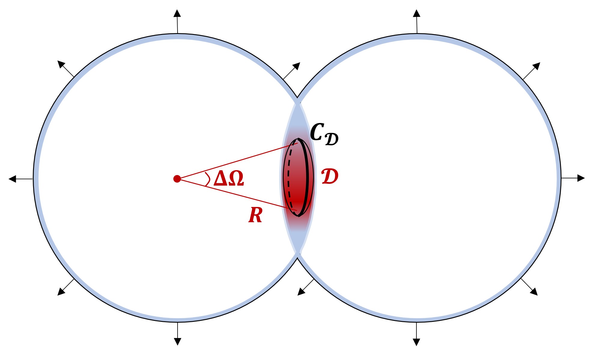
Figure 1: Collision of two bubbles. The bubble walls come with thick fluid shells indicated by light blue. The red region indicated by ${\cal D}$ describes the energetically dense region that will collapse and form a PBH. $C_{\cal D}$ denotes the maximum circumference of ${\cal D}$, while $R$ and $\Delta\Omega$ denote the distance to and solid angle of ${\cal D}$ from the center of one of the bubbles.

Therefore, we must have $R\gtrsim\!H^{-1}$ to have any chance of satisfying (3). For $R\gtrsim\!H^{-1}$, we must carefully take into account the curvature of the spacetime and define what we mean by $R$. We should also pay attention to causal relations between the two bubbles.

The necessity for $R\gtrsim\!H^{-1}$ has important physical implications for the nature of the phase transition. On the one hand, in order for such large bubbles to have grown so much by eating up the false vacuum energy, the universe must have been in the false vacuum for a long time. On the other hand, for a successful completion of the phase transition without eternal inflation, the universe must be filled in by many small bubbles quickly. The latter means that the nucleation time $t_{\rm n}$ (i.e., when one or more bubbles begin to pop up in every horizon) must not be too different from the end time $t_{\rm f}$ of the transition, i.e., $t_{\rm f}-t_{\rm n}\lesssim O(H^{-1})$. The former then requires that those large bubbles must have been growing for a long time before $t_{\rm n}$, so the universe must have been in the false vacuum, or in a supercooled phase, for a long duration before $t_{\rm n}$.

To summarize, PBH formation from bubble collisions require near-horizon-sized bubbles with a thick fluid shell. This means that the scalar field responsible for the phase transition must possess the following three properties. First, it must have sufficient couplings to other particles to generate a thick fluid shell on bubble walls. Second, it must give rise to a long supercooled phase upon the phase transition. Third, the potential barrier between the true and false vacua must decrease sufficiently rapidly as the temperature drops after $t=t_{\rm n}$ to ensure a successful percolation of the true vacuum without eternal inflation.

Effects of spacetime curvature for large bubbles: Here we discuss how the naive expressions (2) and (3) should be modified for horizon-sized bubbles to take into account the spacetime curvature.

Fig. 2 schematically shows the structure of one of the colliding bubbles before the collision, where $\mathcal{H}_{\rm t}$ is the 3d hypersurface given by the trajectory of the outer surface of the shell, and $\mathcal{H}_{\rm s}(R)$ is a spacelike 3d hypersurface on which the bubble appears spherically symmetric with radius $R$, where $R$ is defined such that the area of the intersection of $\mathcal{H}_{\rm s}(R)$ and $\mathcal{H}_{\rm t}$ is given by $4\pi R^{2}$. Finally, $\mathcal{V}_{\rm 4b}$ denotes the 4d world-volume of the bubble shell bounded by $\mathcal{H}_{\rm s}(R)$.

Then, in (2), the naive factor of $4\pi R^{3}\Delta V/3$ representing the total energy of a single bubble with radius $R$ should be replaced as

$$\frac{4\pi R^{3}}{3}\Delta V\>\longrightarrow\>E(R)\equiv\int_{\mathcal{H}_{\rm s}(R)}\mathrm{d}^{3}x\sqrt{\gamma}\;T^{\mu\nu}N_{\mu}N_{\nu}\,,$$ (4)

where $T^{\mu\nu}$ is the energy-momentum tensor, $\gamma_{\mu\nu}$ denotes the 3d metric on $\mathcal{H}_{\rm s}(R)$, and $N_{\mu}$ is a normalized timelike 4-vector field orthogonal to $\mathcal{H}_{\rm s}(R)$.

To calculate $E(R)$, we make use of the Gauss theorem on $\nabla_{\!\mu}(T^{\mu\nu}v_{\nu})$, where $v^{\mu}$ is a timelike 4-velocity field with the boundary condition that $v^{\mu}=N^{\mu}$ on $\mathcal{H}_{\rm s}(R)$. (The boundary condition of $v^{\mu}$ at $\mathcal{H}_{\rm t}$ will be specified later.) Then, $E(R)$ can be rewritten as

$$E(R)=\!\int_{\mathcal{H}_{\rm t}}\mathrm{d}^{3}x\sqrt{-\gamma}\,n_{\mu}T^{\mu\nu}v_{\nu}+\!\int_{\mathcal{V}_{\rm 4b}}\mathrm{d}^{4}x\sqrt{-g}\,\nabla_{\!\mu}(T^{\mu\nu}v_{\nu}),$$ (5)

where $n_{\mu}$ is a normalized spacelike 4-vector field orthogonal to $\mathcal{H}_{\rm t}$ and pointing inward into the bubble. We have set $T^{\mu\nu}=0$ in the interior of the bubble (i.e., between $\mathcal{H}_{\rm s}(R)$ and the inner surface of the shell ${\cal V}_{\rm 4b}$), where the spacetime is in the true vacuum.

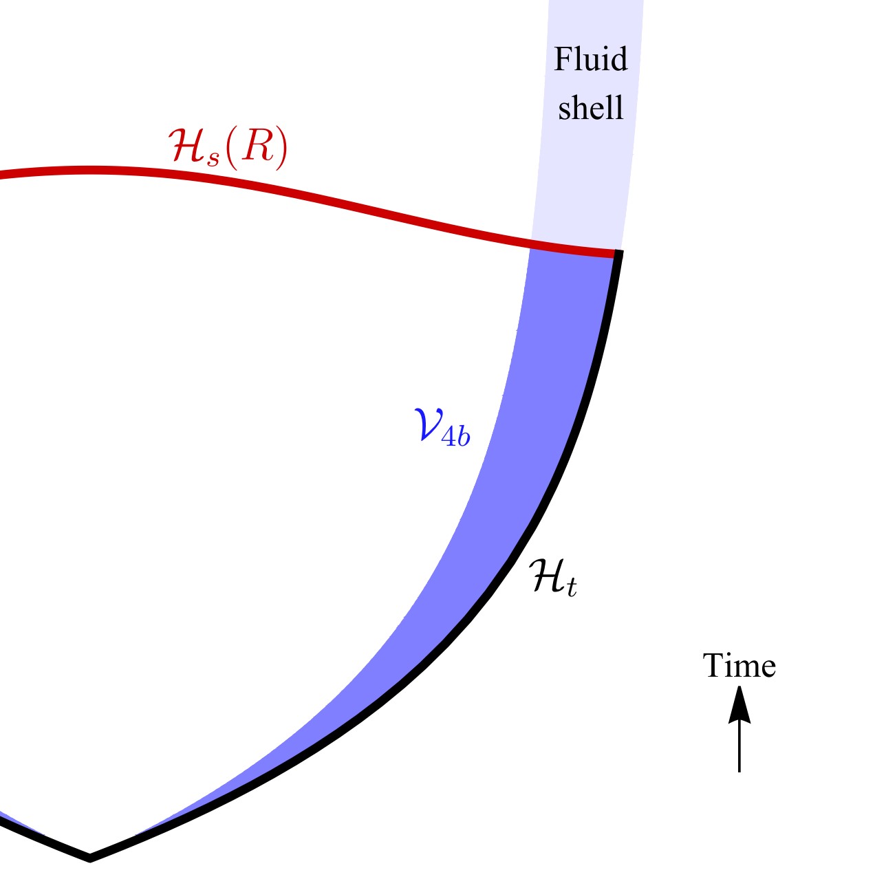
Figure 2: Schematic picture of a single bubble expansion. ${\cal H}_{\rm s}(R)$ is a spacelike hypersurface on which the bubble appears spherically symmetric with radius $R$, ${\cal H}_{\rm t}$ is the hypersurface along the outer surface of the shell, and ${\cal V}_{\rm 4b}$ is the world volume of the fluid shell bounded by $\mathcal{H}_{\rm s}(R)$.

While we cannot calculate the $\mathcal{V}_{\rm 4b}$ term in (5) without a numerical simulation of the bubble shell, the $\mathcal{H}_{\rm t}$ term can be analytically evaluated as follows. Since the exterior of bubbles must be in a highly supercooled phase as we discussed earlier, we can approximate $T^{\mu\nu}$ outside $\mathcal{H}_{\rm t}$ as $T^{\mu\nu}=-\Delta Vg^{\mu\nu}$. Then, the metric outside $\mathcal{H}_{\rm t}$ can be approximated as de Sitter:

$$\mathrm{d}s^{2}=-\mathrm{d}t^{2}+\mathrm{e}^{2Ht}\bigl{[}\mathrm{d}r^{2}+r^{2}(\mathrm{d}\theta^{2}+\sin^{2\!}\theta\,\mathrm{d}\phi^{2})\bigr{]}$$ (6)

with $H^{2}=8\pi G\Delta V/3$, where, without loss of generality thanks to the symmetry of the de Sitter spacetime, we have chosen the coordinate system in which the bubble appears spherically symmetric. We take $v^{\mu}$ on and outside $\mathcal{H}_{\rm t}$ to be at rest in this coordinate system. While the value of $E(R)$ evidently depends on the choice of $v^{\mu}$, our choice is arguably the most natural one. With this choice and in the de Sitter approximation, the calculation detailed in Sec. S1 of Supplemental Material gives

$$\int_{\mathcal{H}_{\rm t}}\mathrm{d}^{3}x\sqrt{-\gamma}\,n_{\mu}T^{\mu\nu}v_{\nu}\>=\>-4\pi\Delta V\!\int_{0}^{r_{0}}\mathrm{d}r\;r^{2}\mathrm{e}^{3Ht(r)}\,,$$ (7)

where $t(r)$ describes $\mathcal{H}_{\rm t}$ as a function of $r$, and $r_{0}$ is given via $R=r_{0}\mathrm{e}^{Ht(r_{0})}$. The strongly supercooled universe permits us to approximate that the bubble expands at the speed of light, i.e., $\mathrm{d}r=\mathrm{e}^{-Ht}\mathrm{d}t$ on $\mathcal{H}_{\rm t}$, which gives $\mathrm{e}^{Ht(r)}=1/(1-Hr)$. With this approximation, the right-hand side of (7) becomes

$$-4\pi\Delta V\frac{1}{H^{3}}\!\left[\frac{H^{2}R^{2}}{2}-HR+\ln(1+HR)\right].$$ (8)

This is negative for all values of $HR$, which in the large $HR$ limit approaches to

$$-\frac{4\pi R^{3}}{3}\Delta V\frac{3}{2HR}\,.$$ (9)

We can now estimate $E(R)$ as follows. Since the $\mathcal{H}_{\rm t}$ contribution in (5) is negative, the $\mathcal{V}_{\rm 4b}$ contribution must be positive with its order of magnitude being at least that of the $\mathcal{H}_{\rm t}$ contribution in order for $E(R)$ to be positive. We can thus use the magnitude of (9) as our estimate of $E(R)$ for $HR\gtrsim 1$. Since we want conditions for PBH formation, this estimate will lead to conservative conditions unless there is a fine cancellation between the positive and negative contributions, which seems extremely unlikely because the $\mathcal{V}_{\rm 4b}$ contribution would depend on the details of the bubble structure and dynamics while the $\mathcal{H}_{\rm t}$ contribution does not, as our above calculation shows.

We thus conclude that we have

$$E(R)\sim\frac{4\pi R^{3}}{3}\Delta V\frac{1}{HR}\,$$ (10)

for $HR\gtrsim 1$, implying that (2) should be modified as

$$M\sim 2\kappa\cdot\frac{4\pi R^{3}}{3}\Delta V\frac{1}{HR}\cdot\frac{\Delta\Omega}{4\pi}\,.$$ (11)

The naive criterion (3) is then corrected as

$$1\lesssim\kappa HR\sqrt{\frac{\Delta\Omega}{4\pi}}\,.$$ (12)

This is one of the main results of this work. We did not modify our guesstimate for the circumference $C_{\cal D}$, because $C_{\cal D}$ is measured outside the dense region that may form a PBH so we can still use the flat-space guesstimate of $C_{\cal D}$ as a good approximation. Similarly, we did not modify the definition of $\Delta\Omega$ as the solid angle seen from the center in the interior of the bubble as the spacetime is approximately flat there.

PBH mass spectrum: Combining the PBH mass (11) with the inequality (12), we get $M_{\mathrm{PBH}}\gtrsim\frac{8\pi}{3\kappa}H^{-3}\Delta V$. We expect this inequality to be saturated because larger bubbles have to be born earlier but the bubble nucleation rates at earlier times are more exponentially suppressed than those for the bubbles that are barely large enough to satisfy (12). Therefore, we predict that the PBH mass spectrum should be monochromatic at the value given by the threshold of the above inequality:

$$M_{\mathrm{PBH}}\approx\frac{8\pi}{3\kappa}H^{-3}\Delta V\,.$$ (13)

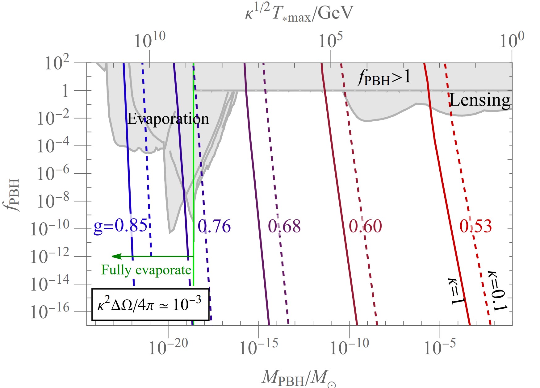
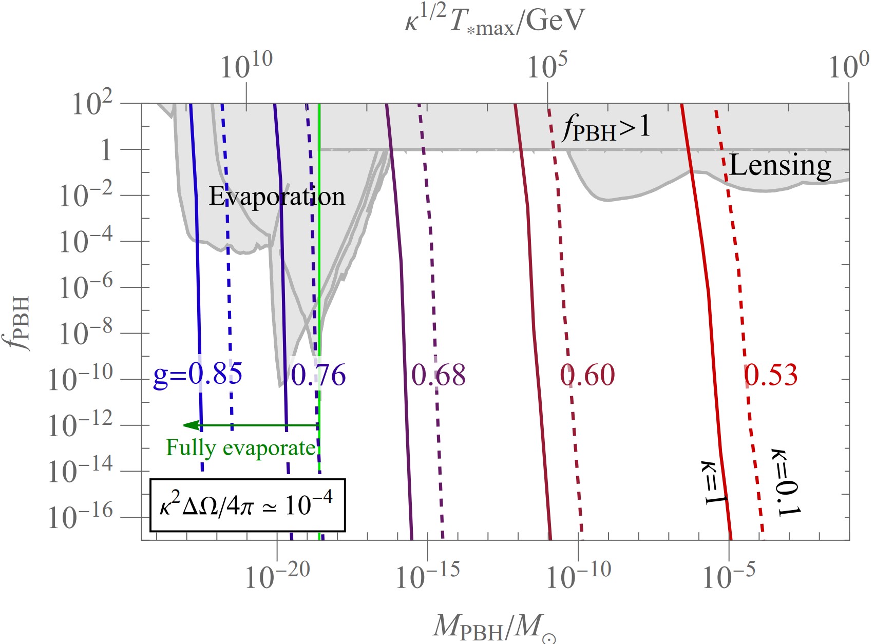
Figure 3: The predicted relation between the PBH abundance $f_{\mathrm{PBH}}$ and $M_{\mathrm{PBH}}$ (bottom axis) or $\sqrt{\kappa}\,T_{*\mathrm{max}}$ (top axis) for $\kappa^{2}\Delta\Omega/4\pi=10^{-3}$ (left), and $10^{-4}$ (right). The relation further depends on the U(1) gauge coupling $g$ and the parameter $\kappa$. Different values of $g$ are represented by lines of different colors, where for each color two different values of $\kappa$ are represented by solid ($\kappa=1$) and dashed ($\kappa=0.1$) lines. These results are for $T_{*}=T_{*\mathrm{max}}$ and $g_{*}=g_{*{\rm SM}}$. The $T_{*}$ and $g_{*}$ dependencies can be obtained by simple rescaling. Current observational constraints, taken from [61, 62], are depicted by gray shaded regions. The vertical axis in each pane denotes the values of $f_{\mathrm{PBH}}$ that we would observe today if we ignored Hawking evaporation, and the PBHs lighter than $M_{\mathrm{PBH}}=5\times 10^{14}\>{\rm g}$ [81, 82] (depicted by the green solid vertical line) would actually have fully evaporated by today.

PBH abundance: We now have all ingredients necessary to estimate $f_{\mathrm{PBH}}\equiv M_{\mathrm{PBH}}\,n_{\mathrm{PBH}}/\rho_{\mathrm{DM}}$. We have the prediction of mass (13) and, as it is derived in Sec. S2 of Supplemental Material, $n_{\mathrm{PBH}}$ is given by

$$n_{\mathrm{PBH}}\sim\int_{t_{\mathrm{c}}}^{t_{\rm f}}\mathrm{d}t\;\mathrm{e}^{3H(t-t_{\rm f})}\,\Gamma_{\rm n}(t)\,P_{\mathrm{PBH}}(t)\,,$$ (14)

where $P_{\mathrm{PBH}}(t)$ is the probability for a bubble born at time $t$ to eventually collide with another bubble and form a PBH, $\Gamma_{\rm n}(t)$ is the bubble nucleation rate per unit volume at time $t$, and $t_{\rm f}$ is the end of the phase transition. The definition of $t_{\rm f}$ and the form of $P_{\mathrm{PBH}}(t)$ are discussed in Sec. S2 of Supplemental Material, and in particular the latter depends on the criterion (12) in an essential way.

For the reader familiar with the literature, we should mention that we do not adopt the commonly used parametrization for $\Gamma_{\rm n}$ proposed by [118, 17]: $\Gamma_{\rm n}(t)=H^{4}\mathrm{e}^{\beta(t-t_{\rm n})}$, where $\beta$ is a free parameter and $t_{\rm n}$ the nucleation time. The reason is the following. This parametrization is essentially a Taylor expansion around $t=t_{\rm n}$ in the exponent, so it is a good model-independent parametrization if $t$ is sufficiently near $t_{\rm n}$. But we are interested in large bubbles that were born much earlier than $t_{\rm n}$, so the Taylor expansion is not justified. Since there is no good model-independent way to parametrize $\Gamma_{\rm n}(t)$ at such early times, we must choose a benchmark model. We adopt a simple Abelian Higgs model as our benchmark because, as we already mentioned, a thick fluid shell may be realized by a phase transition that breaks gauge symmetry, and the phase transition can be made strongly first order. The benchmark model is described in detail in Sec. S3 of Supplemental Material.

Next, we treat $\kappa$ and $\kappa^{2}\Delta\Omega$ as free parameters because we would need detailed numerical relativity+fluid dynamics simulations to calculate them, which we save for future work. The reason for treating the combination $\kappa^{2}\Delta\Omega$ as an independent parameter rather than $\Delta\Omega$ itself is because the PBH formation criterion (12) depends only on the combination $\kappa^{2}\Delta\Omega$ and not on $\kappa$ or $\Delta\Omega$ separately, so the PBH number density depends only on $\kappa^{2}\Delta\Omega$. On the other hand, the PBH mass depends only on $\kappa$ in (13). There is still a potentially serious complication that in reality $\kappa$ and $\kappa^{2}\Delta\Omega$ are likely to depend also on the quantities that vary collision-by-collision like the time elapsed since $t_{\rm n}$, the bubble radii at the time of the collision, etc. In this work we ignore this complication and use the same values of $\kappa$ and $\kappa^{2}\Delta\Omega$ for all collisions.

Lastly, the reheating temperature $T_{*}$ is also a free parameter. Reheating occurs as the phase transition ends by a large number of small bubbles colliding and filling up the universe with the true vacuum, during which the energy of the bubble shells, which were originally the false vacuum energy, are being converted to heat in the plasma permeating in the true vacuum. Since this end stage of the phase transition is not instantaneous but lasts for a time of $O(H^{-1})$, not 100% of the original energy of the false vacuum would be converted to heat but some fraction of it would be lost to the expansion of the universe. The value of $T_{*}$ also depends on $g_{*}$, the radiation degrees of freedom at $T=T_{*}$, which is necessarily larger than that of the SM, $g_{*{\rm SM}}=106.75$. Therefore, we have $T_{*}<T_{*\mathrm{max}}$, where $T_{*\mathrm{max}}$ is defined via $\frac{\pi^{2}}{30}g_{*\rm SM}T_{*\mathrm{max}}^{4}=\Delta V$. Since the value of $T_{*}$ depends on details of the model and reheating dynamics, in this work we treat $T_{*}$ as a free parameter bounded by $T_{*{\rm max}}$.

With these limitations in mind, we show in Fig. 3 our results for the PBH abundance $f_{\mathrm{PBH}}$ vs the PBH mass $M_{\mathrm{PBH}}$ for several benchmark values of $\kappa^{2}\Delta\Omega/4\pi$. Since $M_{\mathrm{PBH}}$ and $\sqrt{\kappa}\,T_{*\mathrm{max}}$ has a one-to-one correspondence (see Sec. S2.3 of Supplemental Material), we also show the values of $\sqrt{\kappa}\,T_{*\mathrm{max}}$ in the upper horizontal axes. At given $M_{\mathrm{PBH}}$ or $\sqrt{\kappa}\,T_{*\mathrm{max}}$, the abundance depends on the U(1) gauge coupling constant $g$ of the Abelian Higgs benchmark model and also on $\kappa$. Different values of $g$ are distinguished by lines of different colors, while different values of $\kappa$ are shown in lines of different forms (solid or dashed). To avoid too much clatter in the plots, we show the results only for $T_{*}=T_{*\mathrm{max}}$, and $g_{*}=g_{*{\rm SM}}$. There is no real loss of generality, however, because both $M_{\mathrm{PBH}}$ and $f_{\mathrm{PBH}}$ scale very simply in terms of $g_{*}/g_{*{\rm SM}}$ and $T_{*}/T_{*\mathrm{max}}$. As shown in Sec. S2.3 of Supplemental Material, $f_{\mathrm{PBH}}$ should be multiplied by $(T_{*\mathrm{max}}/T_{*})^{3}(g_{*{\rm SM}}/g_{*})$. The dependences of $f_{\mathrm{PBH}}$ on $\kappa$ and $\kappa^{2}\Delta\Omega$ are very complicated as discussed in detail in Sec. S2.1 of Supplemental Material, and it is not possible to express them by simple re-scalings.

The vertical axes in Fig. 3 represent the values of $f_{\mathrm{PBH}}$ that we would observe if we ignored the evaporation of the PBHs by Hawking radiation [119, 120]. As discussed in [81, 82], the PBHs lighter than about $5\times 10^{14}\,{\rm g}$ (indicated by the green solid vertical line in each pane of Fig. 3) would have fully evaporated by today.

The gray regions in Fig. 3 represent constraints on $f_{\mathrm{PBH}}$ taken from [61, 62]. The PBH abundance in the mass range of $10^{-10}M_{\odot}\lesssim M_{\mathrm{PBH}}\lesssim 10M_{\odot}$, corresponding to $0.1\,\mathrm{GeV}\lesssim\sqrt{\kappa}\,T_{*\mathrm{max}}\lesssim 10^{5}\,\mathrm{GeV}$, is constrained by gravitational lensing [63, 64, 65, 66, 67, 68, 69, 70, 71, 72, 73, 74, 75, 76, 77, 78, 79], while the range below $10^{-16}M_{\odot}$, corresponding to $\sqrt{\kappa}\,T_{*\mathrm{max}}\gtrsim 10^{8}\,\mathrm{GeV}$, is strongly constrained by Hawking evaporation as those PBHs would have partially or fully evaporated with observable signals in various channels [80, 81, 82, 83, 84, 85, 86, 87, 88, 89, 90]. Those in the range $M_{\mathrm{PBH}}\lesssim 10^{-19}M_{\odot}$ (or $\sqrt{\kappa}\,T_{*\mathrm{max}}\gtrsim 10^{9}\,\mathrm{GeV}$) on the left of the green solid line would have completely evaporated by today [81, 82] so they could not constitute dark matter even if we disregarded the evaporation signals.

The most interesting range for us is $10^{-16}M_{\odot}\lesssim M_{\mathrm{PBH}}\lesssim 10^{-10}M_{\odot}$, corresponding to $10^{5}\,\mathrm{GeV}\lesssim\sqrt{\kappa}\,T_{*\mathrm{max}}\lesssim 10^{8}\,\mathrm{GeV}$, which is currently unconstrained by any PBH searches. The value of the U(1) gauge coupling $g$ only needs to be mildly tuned to 10% level to have $f_{\mathrm{PBH}}=1$ in this mass window. But as we can see from the steepness of the colored lines in Fig. 3, the value of $f_{\mathrm{PBH}}$ for given $g$ is exponentially sensitive to $M_{\mathrm{PBH}}$ or the overall mass scale of the theory. This seems inevitable in our scenario not only because our PBH production is due to large bubbles that were born long before $t_{\rm n}$ and hence extremely rare, but also because the rarity itself, $\Gamma_{\rm n}$, is exponentially sensitive to the underlying parameters of the theory. Therefore, we conclude that

• Dark matter may be (entirely) comprised of PBHs of a monochromatic mass spectrum produced from bubble collisions during a cosmological first-order phase transition in a rather mundane field theory like a U(1) gauge theory with an $O(1)$ gauge coupling spontaneously broken at an intermediate energy scale above the electroweak scale.

• At the same time, it is highly non-generic to land near $f_{\mathrm{PBH}}=1$ and/or in the allowed window of $M_{\mathrm{PBH}}$, so PBH production from bubble collisions can put severe constraints on field-theoretic models with cosmological first-order phase transitions.

These are the main messages of our work.

Prospects for future work: While we have shown that bubble collisions during a first-order phase transition could produce a sizable abundance of PBHs or even over-close the universe, there are a few important loose ends that need to be worked out in future work. The first important problem is to understand the dynamics of a single, large bubble, especially the friction on the expanding bubble wall and the thickness of the fluid shell, because a macroscopically thick fluid shell is necessary for PBH production. The challenge is to study this in a curved spacetime, because our bubbles are near horizon-sized.

Next step will be to perform a numerical relativity simulation of collision of two large bubbles to get the parameters $\kappa$ and $\kappa^{2}\Delta\Omega$. It will be also interesting and important to simulate collisions of many small bubbles to study reheating. Recall that PBHs are produced from rare collisions of large bubbles, while nearly all collisions are collisions of small bubbles happening near the end of the phase transition, which reheat the universe. The question is how close $T_{*}$ is to $T_{*\mathrm{max}}$.

Another direction is to explore other benchmarks. While our U(1) benchmark model appears to be one of the simplest possible models, it is completely an independent module and not connected to the Standard Model. Perhaps it would be more satisfactory if it is more integrated into a bigger structure including the Standard Model and other crucial elements such as inflation.

As for PBH signals and constraints, the currently open region between $10^{-16}M_{\odot}$ and $10^{-10}M_{\odot}$ may be partly probed through Hawking evaporation by future MeV gamma-ray telescopes [121, 122, 123] such as AdEPT [124], AMEGO [125], eASTROGAM [126], GECCO [127], MAST  [128], PANGU [129], GRAMS [130] and XGIS [131, 132], as well as through a future extension of the analysis of Ref. [69] with more data. This region may also be covered by future gravitational wave experiments because first-order phase transitions with $t_{\rm f}-t_{\rm n}$ comparable to $H^{-1}$ like in our scenario can enhance gravitational wave production [19, 20]. Moreover, such phase transition can lead to a distribution of bubble radii that may give rise to distinct features in the gravitational wave spectrum. We leave these interesting questions for future work.

Acknowledgement: THJ thanks Chang Sub Shin for helpful discussions regarding the hoop conjecture. We also thank Kiyoharu Kawana for his valuable feedback and discussions on our earlier version of the paper. This work is supported by the US Department of Energy (DOE) grant DE-SC0010102, by the Japan Society for Promotion of Science (JSPS) grant KAKENHI 21H01086, and by the Institute for Basic Science (IBS) under the project code IBS-R018-D1.

Primordial black holes from bubble collisions during a first-order phase transition
Supplemental Material
Tae Hyun Jung and Takemichi Okui

S1 Derivation of Eq. (7)

As discussed in the main text around Eq. (6), we take the metric outside the outer surface of the bubble shell, $\mathcal{H}_{\rm t}$, to be given by (6). Since the hypersurface $\mathcal{H}_{\rm t}$ does not appear simple in this coordinate system, we consider the following coordinate transformation:

$$\!\begin{pmatrix}\mathrm{d}t\\ \mathrm{d}r\\ \mathrm{d}\theta\\ \mathrm{d}\phi\end{pmatrix}\!=\!\begin{pmatrix}\mathrm{e}^{Ht}&\mathrm{e}^{Ht}v&0&0\\ v&1&0&0\\ 0&0&1&0\\ 0&0&0&1\end{pmatrix}\!\!\begin{pmatrix}\mathrm{d}t^{\prime}\\ \mathrm{d}r^{\prime}\\ \mathrm{d}\theta^{\prime}\\ \mathrm{d}\phi^{\prime}\end{pmatrix}\!\equiv\Lambda\!\begin{pmatrix}\mathrm{d}t^{\prime}\\ \mathrm{d}r^{\prime}\\ \mathrm{d}\theta^{\prime}\\ \mathrm{d}\phi^{\prime}\end{pmatrix}\!.$$ (S.1)

The primed coordinates are valid only in an infinitesimal region of $\mathcal{H}_{\rm t}$ around a given point on $\mathcal{H}_{\rm t}$. Let us call this infinitesimal region $\delta\mathcal{H}_{\rm t}$, and $v$ is constant within $\delta\mathcal{H}_{\rm t}$. We would like $\delta\mathcal{H}_{\rm t}$ to be locally described as a surface on which $\mathrm{d}r^{\prime}=0$. Through (S.1), this corresponds to $v=\mathrm{e}^{Ht}\mathrm{d}r/\mathrm{d}t$. Thus, $v$ can be interpreted as the “proper speed” of the expansion of the bubble’s outer surface as measured in the unprimed coordinates under the metric (S.2). In other words, the primed coordinates can be regarded as the instantaneous rest frame of a point on the outer surface. Since $\Lambda$ is not invertible at $v=1$, we take $v$ in the range $0\leq v<1$, which is also physical because the bubble expansion speed is near 1 but not exactly 1.

In (S.1), the $\Lambda^{t}_{~{}t^{\prime}}$ component has been chosen such that $t^{\prime}$ would be the conformal time, while the $\Lambda^{r}_{~{}r^{\prime}}$ component has been chosen such that $\mathrm{d}r=\mathrm{d}r^{\prime}$ on any spacelike 3d hypersurface with a constant $t^{\prime}$. The $\Lambda^{r}_{~{}t^{\prime}}$ component simply defines $v$ as discussed above. The $\Lambda^{t}_{~{}r^{\prime}}$ component has been chosen such that the metric remains diagonal in the primed coordinates:

$$(g_{\mu^{\prime}\nu^{\prime}})=\Lambda^{\mathrm{\!T}}\!\begin{pmatrix}-1&0&0&0\\ 0&\mathrm{e}^{2Ht}&0&0\\ 0&0&\mathrm{e}^{2Ht}r^{2}&0\\ 0&0&0&\mathrm{e}^{2Ht}r^{2}\sin^{2\!}\theta\end{pmatrix}\!\Lambda=\!\begin{pmatrix}-\mathrm{e}^{2Ht}(1-v^{2})&0&0&0\\ 0&\mathrm{e}^{2Ht}(1-v^{2})&0&0\\ 0&0&\mathrm{e}^{2Ht}r^{2}&0\\ 0&0&0&\mathrm{e}^{2Ht}r^{2}\sin^{2\!}\theta\end{pmatrix}\!.$$ (S.2)

Now, since $\mathrm{d}r^{\prime}=0$ on $\delta\mathcal{H}_{\rm t}$, the 3d induced metric in $\delta\mathcal{H}_{\rm t}$ can be immediately read off from (S.2) by removing the second row and second column from it:

$$(\gamma_{\mu^{\prime}\nu^{\prime}})=\!\begin{pmatrix}-\mathrm{e}^{2Ht}(1-v^{2})&0&0\\ 0&\mathrm{e}^{2Ht}r^{2}&0\\ 0&0&\mathrm{e}^{2Ht}r^{2}\sin^{2\!}\theta\end{pmatrix}\!,$$ (S.3)

where $\mu^{\prime},\nu^{\prime}=t^{\prime},\theta^{\prime},\phi^{\prime}$. Hence,

$$\sqrt{-\gamma^{\prime}}=\mathrm{e}^{3Ht}\sqrt{1-v^{2}}\,r^{2}\sin\theta\,.$$ (S.4)

In the primed coordinates, the normal vector on $\delta\mathcal{H}_{\rm t}$ can also be easily found from (S.2):

$$(n_{\mu\prime})=(0,-\mathrm{e}^{Ht}\sqrt{1-v^{2}},0,0)\,,$$ (S.5)

where the negative sign is due to our convention that this vector should point inward from $\mathcal{H}_{\rm t}$ into $\mathcal{V}_{\rm 4b}$. We also need $v^{\mu}$, which is by definition the 4-velocity of the observer who has been outside of the bubble and at rest in the unprimed coordinates. So, it is given in the primed coordinates at $\delta\mathcal{H}_{\rm t}$ by

$$(v^{\mu\prime})=\Lambda^{\!-1}\!\begin{pmatrix}1\\ 0\\ 0\\ 0\end{pmatrix}\!=\frac{1}{\mathrm{e}^{Ht}(1-v^{2})}\!\begin{pmatrix}1\\ -v\\ 0\\ 0\end{pmatrix}\!.$$ (S.6)

Hence, with our approximation $T^{\mu\nu}=-\Delta Vg^{\mu\nu}$ on $\mathcal{H}_{\rm t}$, we have

$$n_{\mu}T^{\mu\nu}v_{\nu}\>=\>-\Delta V\,n\!\cdot\!v\>=\>-\Delta V\frac{v}{\sqrt{1-v^{2}}}\,,$$ (S.7)

which, together with (S.4), gives

$$\mathrm{d}^{3}x\sqrt{-\gamma}\;n_{\mu}T^{\mu\nu}v_{\nu}\>=\>\mathrm{d}t^{\prime}\,\mathrm{d}\theta^{\prime}\,\mathrm{d}\phi^{\prime}\,\mathrm{e}^{3Ht}\sqrt{1-v^{2}}\,r^{2}\sin\theta\,\frac{-\Delta V\,v}{\sqrt{1-v^{2}}}\>=\>-\Delta V\,\mathrm{d}r\,\mathrm{d}\Omega\;\mathrm{e}^{3Ht}r^{2}\,,$$ (S.8)

where in the last step we have used the relation $\mathrm{d}r=v\,\mathrm{d}t^{\prime}$, which follows readily from (S.1) as $\mathrm{d}r^{\prime}=0$ on $\delta\mathcal{H}_{\rm t}$. Since the rightmost expression in (S.8) no longer has any reference to the primed coordinates or to $\delta\mathcal{H}_{\rm t}$, it can be directly integrated over the entire $\mathcal{H}_{\rm t}$ in the original unprimed coordinates. This concludes the derivation of Eq. (7) of the main text.

S2 The PBH abundance

S2.1 $n_{\mathrm{PBH}}$

In this section, we explain how we estimate the number density of PBHs based on our criterion (12) discussed in the main text.

Consider a bubble that was born at time $t$, and let $P_{\mathrm{PBH}}(t)$ be the probability for this bubble to eventually form a PBH by colliding with another bubble that was born later (and hence younger and smaller). To express the probability for the first, older and bigger, bubble to be born, we introduce $\Gamma_{\rm n}(t)$ as the bubble nucleation rate at time $t$ per unit volume of the false vacuum, and $P_{\rm f}(t)$ as the co-moving 3-volume of false-vacuum regions per unit co-moving 3-volume at time $t$. Then, with our approximation that bubbles are born at rest in the coordinates (6), the final number of PBHs within a large 3-volume ${\rm CoV}_{\!3}$ co-moving with those coordinates is given by

$$N_{\mathrm{PBH}}=\int_{t_{\mathrm{c}}}^{t_{\rm f}}\mathrm{d}t\int_{{\rm CoV}_{\!3}}\mathrm{d}^{3}x\,\sqrt{-g}\;P_{\rm f}(t)\,\Gamma_{\rm n}(t)\,P_{\mathrm{PBH}}(t)\,,$$ (S.9)

where $t_{\rm f}$ marks the end of the PBH formation period (to be defined shortly), while $t_{\mathrm{c}}$ denotes the time corresponding to the critical temperature $T_{\mathrm{c}}$ marking the beginning of the phase transition. Taking ${\rm CoV}_{\!3}$ to be sufficiently large, it is justified to disregard the “fringe effects” of how to count, or not count, the PBHs from the bubbles born near the boundary of ${\rm CoV}_{\!3}$.

Let us now discuss how we should like to define $t_{\rm f}$. Since PBHs are extremely rare, we neglect the curvatures induced by the PBHs and just use the background metric for the $\sqrt{-g}$ factor. As explained in the main text, we have a long super-cooled phase so the background metric remains de Sitter for a long time to allow for the rare and large bubbles to grow, until when a large number of small bubbles begin to form rapidly to bring the whole universe into the true vacuum. The time $t_{\rm f}$ represents this time when small bubbles begin to fill the universe. Clearly there is no way to define such time sharply in a unique manner, but one reasonable definition may be motivated by observing that the ratio of the volume of a sphere of diameter $\ell$ to that of a cube of side $\ell$ is given by $\pi/6\simeq 1/2$. On average, when the volume fraction of small bubbles begin to exceed this ratio, some of the small bubbles must collide and overlap with one another, initiating the end of the phase transition (which must complete rapidly to avoid eternal inflation). We thus define $t_{\rm f}$ as

$$P_{\rm f}(t_{\rm f})\equiv\frac{1}{2}\,.$$ (S.10)

With this and the approximation of taking the background metric to be de Sitter before $t_{\rm f}$, we estimate $N_{\mathrm{PBH}}$ as

$$N_{\mathrm{PBH}}\sim\int_{t_{\mathrm{c}}}^{t_{\rm f}}\mathrm{d}t\int_{{\rm CoV}_{\!3}}\mathrm{d}^{3}x\;\mathrm{e}^{3Ht}\,\Gamma_{\rm n}(t)\,P_{\mathrm{PBH}}(t)\,.$$ (S.11)

To get the PBH number density $n_{\mathrm{PBH}}$, we divide this by the volume of ${\rm CoV}_{\!3}$ at $t=t_{\rm f}$:

$$n_{\mathrm{PBH}}\sim\frac{\displaystyle{\int_{t_{\mathrm{c}}}^{t_{\rm f}}\mathrm{d}t\;\mathrm{e}^{3Ht}\,\Gamma_{\rm n}(t)\,P_{\mathrm{PBH}}(t)}}{\mathrm{e}^{3Ht_{\rm f}}}\>=\>\int_{t_{\mathrm{c}}}^{t_{\rm f}}\mathrm{d}t\;\mathrm{e}^{3H(t-t_{\rm f})}\,\Gamma_{\rm n}(t)\,P_{\mathrm{PBH}}(t)\,.$$ (S.12)

But we should emphasize that the definition of $t_{\rm f}$ has an intrinsic arbitrariness of $O(H^{-1})$ and, therefore, the above estimate has an uncertainty of $O(\mathrm{e}^{\pm\text{a few}})$.

In (S.12), $\Gamma_{\rm n}(t)$ is a quantity that should be computed in quantum field theory once the scalar sector responsible for the phase transition is specified, which we will discuss in section S3. Here, our task is to find $P_{\mathrm{PBH}}(t)$, namely, the probability for a bubble born at time $t$ to collide with another bubble born later and form a PBH. Since $\Gamma_{\rm n}(t)$ is the conditional probability for a bubble to form per unit volume per unit time given that the volume is in the false vacuum and $P_{\rm f}(t)$ is the co-moving volume of false vacuum regions per unit co-moving volume at time $t$, we can express $P_{\mathrm{PBH}}(t)$ in the coordinate system (6) as

$$P_{\mathrm{PBH}}(t_{1})=\int_{t_{1}}^{t_{\rm f}}\!\!\!\mathrm{d}t_{2}\int_{r_{\rm min}}^{r_{\rm max}}\mathrm{d}r\;4\pi r^{2}\,\mathrm{e}^{3Ht_{2}}\,P_{\rm f}(t_{\rm coll})\,\Gamma_{\rm n}(t_{2})\,,$$ (S.13)

where $t_{1}$ ($t_{2}$) is the time when the older (younger) bubble was born, $r$ denotes the co-moving distance between the birth location of the younger bubble and that of the older, and $t_{\rm coll}$ is the time when the two bubbles collide. The limits $r_{\rm min}$ and $r_{\rm max}$ provide the range of $r$ in which the criterion (12) of the main text is satisfied. The presence of $P_{\rm f}(t_{\rm coll})$ discounts the PBH production if the universe is (partially) in the true vacuum at the time of the collision. This is necessary because the bubbles grow and acquire mass by eating up the energy of the false vacuum.

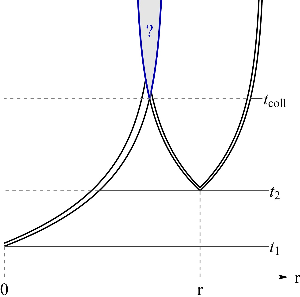
Figure S-1: The collision of two bubbles where with the coordinates and metric outside the bubbles are given by Eq. (6) of the main text. A PBH forms in the region with “?” if our criterion (12) is satisfied. Constant time hypersurfaces are denoted by dashed lines inside the bubbles, as opposed to solid lines, to indicate the fact that the coordinate system used in (6) is defined and used only outside the bubbles.

Let’s now find $r_{\rm min}$ and $r_{\rm max}$. Since we are approximating bubble trajectories as lightlike, they satisfy $\mathrm{d}r=e^{-Ht}\mathrm{d}t$ under the metric (6) of the main text. Then, the co-moving radii $r_{1}$ and $r_{2}$ of the older and younger bubbles at the moment of the collision are given by

$$Hr_{1} =\mathrm{e}^{-Ht_{1}}-\mathrm{e}^{-Ht_{\rm coll}}\,,$$ (S.14)

$$Hr_{2} =\mathrm{e}^{-Ht_{2}}-\mathrm{e}^{-Ht_{\rm coll}}\,.$$

Then, since $r_{1}+r_{2}=r$ by definition, we find

$$\mathrm{e}^{-Ht_{\rm coll}}=\frac{1}{2}(\mathrm{e}^{-Ht_{1}}+\mathrm{e}^{-Ht_{2}}-Hr)\,.$$ (S.15)

Recall that the physical radius $R$ appearing in the criterion (12) is defined such that the surface area of a sphere of radius $R$ is given by $4\pi R^{2}$. Thus, under the metric (6) outside the bubbles, the physical radii $R_{i}$ corresponding to $r_{i}$ ($i=1,2$) at the moment of the collision are given by $R_{i}=r_{i}\,\mathrm{e}^{Ht_{\rm coll}}$. Then, from (S.14) and (S.15), we find

$$H\!R_{1}=\frac{\mathrm{e}^{-Ht_{1}}-\mathrm{e}^{-Ht_{2}}+Hr}{\mathrm{e}^{-Ht_{1}}+\mathrm{e}^{-Ht_{2}}-Hr}\,,\quad H\!R_{2}=\frac{-\mathrm{e}^{-Ht_{1}}+\mathrm{e}^{-Ht_{2}}+Hr}{\mathrm{e}^{-Ht_{1}}+\mathrm{e}^{-Ht_{2}}-Hr}\,.$$ (S.16)

In the criterion (12), we assumed that the two bubbles have an equal radius $R$ for simplicity. Here, since the bubbles have different radii, we should use the smaller radius $R_{2}$ instead of $R$, and redefine $\Delta\Omega$ as the solid angle of ${\cal D}$ as seen from the center of the smaller bubble. Therefore, with (S.16), the criterion (12) can be expressed as

$$1\lesssim\kappa H\!R_{2}\sqrt{\frac{\Delta\Omega}{4\pi}}\quad\Longleftrightarrow\quad(1+\kappa^{\prime})\mathrm{e}^{-Ht_{1}}+(1-\kappa^{\prime})\mathrm{e}^{-Ht_{2}}\lesssim(1+\kappa^{\prime})Hr\,,$$ (S.17)

where $\kappa^{\prime}\equiv\kappa\sqrt{\Delta\Omega/4\pi}$ for brevity. Since we expect that $\kappa^{\prime}\ll 1$, this is equivalent at $O(\kappa^{\prime})$ to

$$\mathrm{e}^{-Ht_{1}}+(1-2\kappa^{\prime})\mathrm{e}^{-Ht_{2}}\lesssim Hr\,,$$ (S.18)

which gives $r_{\rm min}$ as

$$Hr_{\rm min}\simeq\mathrm{e}^{-Ht_{1}}+\biggl{(}1-2\kappa\sqrt{\frac{\Delta\Omega}{4\pi}}\biggr{)}\mathrm{e}^{-Ht_{2}}\,.$$ (S.19)

On the other hand, $r_{\rm max}$ can be found from (S.15) by taking $t_{\rm coll}$ in (S.15) to infinity:

$$Hr_{\rm max}\simeq\mathrm{e}^{-Ht_{1}}+\mathrm{e}^{-Ht_{2}}\,.$$ (S.20)

One might object to the $t_{\rm coll}\to\infty$ limit because the de Sitter expansion does not last forever as the phase transition ends and the universe becomes radiation dominated. In our treatment this “cutoff” is effectively provided by $P_{\rm f}(t_{\rm coll})$ in (S.13).

S2.2 $P_{\rm f}(t)$

The last remaining ingredient we need to complete the expression (S.13) is $P_{\rm f}(t)$, the co-moving volume of false-vacuum regions per unit co-moving volume at time $t$. We can obtain $P_{\rm f}(\tau)$, where $\tau$ is the conformal time, as follows. Between the times $\tau^{\prime}$ and $\tau^{\prime}+\mathrm{d}\tau^{\prime}$, the number of newly nucleated bubbles per unit co-moving volume is given by $\Gamma_{\rm n}(\tau^{\prime})\cdot a(\tau^{\prime})^{4}\,P_{\rm f}(\tau^{\prime})\,\mathrm{d}\tau^{\prime}$. After the time $\tau^{\prime}$, in any interval between $\tau^{\prime\prime}$ and $\tau^{\prime\prime}+\mathrm{d}\tau^{\prime\prime}$, the bubbles born at $\tau^{\prime}$ grow by “eating” part of the false vacuum. The eaten co-moving volume is given by $P_{\rm f}(\tau^{\prime\prime})\cdot 4\pi r(\tau^{\prime\prime},\tau^{\prime})^{2}\,\mathrm{d}r$, where $r(\tau^{\prime\prime},\tau^{\prime})$ is the co-moving radius at time $\tau^{\prime\prime}$ of a bubble born at time $\tau^{\prime}$, $\mathrm{d}r$ is the growth in $r(\tau^{\prime\prime},\tau^{\prime})$ during the interval $\mathrm{d}\tau^{\prime\prime}$, and the factor of $P_{\rm f}(\tau^{\prime\prime})$ is there because the bubbles cannot eat a volume that is already in the true vacuum. Therefore, we obtain

$$P_{\rm f}(\tau)=1-\int_{\tau_{\mathrm{c}}}^{\tau}\!\!d\tau^{\prime}\,P_{\rm f}(\tau^{\prime})\,a(\tau^{\prime})^{4}\,\Gamma_{\rm n}(\tau^{\prime})\int_{\tau^{\prime}}^{\tau}\!\!d\tau^{\prime\prime}\,P_{\rm f}(\tau^{\prime\prime})\cdot 4\pi r(\tau^{\prime\prime},\tau^{\prime})^{2}\,\frac{\partial r(\tau^{\prime\prime},\tau^{\prime})}{\partial\tau^{\prime\prime}}\,,$$ (S.21)

where, since we approximate the bubble wall trajectories to be lightlike, we have

$$r(\tau^{\prime\prime},\tau^{\prime})\simeq\tau^{\prime\prime}-\tau^{\prime}\quad\text{and}\quad\frac{\partial r(\tau^{\prime\prime},\tau^{\prime})}{\partial\tau^{\prime\prime}}\simeq 1\,.$$ (S.22)

Furthermore, we also approximate that $a(\tau)$ is given by the de Sitter expansion, i.e.,

$$a(\tau)=\frac{a_{0}}{1-Ha_{0}(\tau-\tau_{0})}\,,$$ (S.23)

where for convenience we choose the convention that $\tau_{0}=\tau_{\rm n}$ (the nucleation time) and $a_{0}=1$, although the results are convention independent.

S2.3 $M_{\mathrm{PBH}}$ and $f_{\mathrm{PBH}}$

We would first like to rewrite the prediction of $M_{\mathrm{PBH}}$ (Eq. (13) of the main text) by eliminating $H$ from it using $H^{2}=8\pi\Delta V/(3M_{\mathrm{Pl}}^{2})$ with $M_{\mathrm{Pl}}=1.22\times 10^{19}\>\mathrm{GeV}$, and then eliminating $\Delta V$ in favor of the highest possible reheating temperature $T_{*\mathrm{max}}$ defined via $\Delta V=\frac{\pi^{2}}{30}g_{*{\rm SM}}T_{*\mathrm{max}}^{4}$. This leads to

$$M_{\mathrm{PBH}}=\frac{M_{\mathrm{Pl}}^{3}}{\kappa}\sqrt{\frac{3}{8\pi\Delta V}}=\frac{1}{\kappa}\sqrt{\frac{45}{4\pi^{3}g_{*{\rm SM}}}}\frac{M_{\mathrm{Pl}}^{3}}{T_{*\mathrm{max}}^{2}}\,.$$ (S.24)

For the PBH number density, it is the ratio $n_{\mathrm{PBH}}/H^{3}$ that is most easily obtainable from the method described in Sec. S2.1 by working in the units where $H=1$. Then, multiplying the right-hand side of Eq. (13) of the main text by $n_{\mathrm{PBH}}$ and combining the $H^{-3}$ with $n_{\mathrm{PBH}}$, and then eliminating the $\Delta V$ in favor of $T_{*\mathrm{max}}$, we get

$$f_{\mathrm{PBH}}\equiv\frac{M_{\mathrm{PBH}}\,n_{\mathrm{PBH}}}{\rho_{\mathrm{DM}}}=\frac{8\pi}{3\kappa}\frac{\frac{\pi^{2}}{30}g_{*{\rm SM}}T_{*\mathrm{max}}^{4}}{\rho_{\mathrm{DM}}}\,\frac{n_{\mathrm{PBH}}}{H^{3}}=\frac{2\pi}{\kappa}\frac{T_{*\mathrm{max}}}{\rho_{\mathrm{DM}}/s_{*}}\!\left(\frac{T_{*\mathrm{max}}}{T_{*}}\right)^{\!\!3}\frac{g_{*{\rm SM}}}{g_{*}}\frac{n_{\mathrm{PBH}}}{H^{3}}\,,$$ (S.25)

where we have introduced the entropy density $s_{*}=(2\pi^{2}/45)g_{*}T_{*}^{3}$ at the reheating, and the value of $\rho_{\mathrm{DM}}/s_{*}$ is $\simeq 0.44\>{\rm eV}$ from observation.

S3 The benchmark model and its properties

Here we describe the benchmark model to generate the results presented in the paper.

S3.1 The model

We introduce a complex scalar field $\Phi$ charged under a U(1) gauge symmetry whose gauge field and coupling are $A_{\mu}$ and $g$. We work at 1-loop in dimensional regularization in $4-\epsilon$ dimensions with $\overline{\text{MS}}$ subtraction. Our model is defined in this scheme by the following lagrangian:

$$\mathcal{L}=-({\rm D}_{\!\mu}\Phi)^{*}\,{\rm D}^{\mu}\Phi-\frac{\lambda}{4}|\Phi|^{4}+\frac{1}{g^{2}}\biggl{[}-\frac{1}{4}F^{\mu\nu}F_{\mu\nu}-\frac{1}{2\xi}(\partial_{\mu}A^{\mu})^{2}\biggr{]}+\mathcal{L}_{\rm ct}\,,$$ (S.26)

where ${\rm D}_{\!\mu}\Phi\equiv(\partial_{\mu}-\mathrm{i}A_{\mu})\Phi$, and $\mathcal{L}_{\rm ct}$ denotes the 1-loop counterterms:

$$\mathcal{L}_{\rm ct}=\frac{1}{16\pi^{2}\epsilon}\biggl{[}-2(3-\xi)g^{2}({\rm D}_{\!\mu}\Phi)^{*}\,{\rm D}^{\mu}\Phi-\bigl{(}5\lambda^{2}-4\xi\lambda g^{2}+24g^{4}\bigr{)}\frac{|\Phi|^{4}}{4}+\frac{2}{3}\,\frac{1}{4}F^{\mu\nu}F_{\mu\nu}\biggr{]}\,,$$ (S.27)

where the $1/\epsilon$ poles above are only the UV poles, and the treatment of IR divergence is implicit. The ghost terms are implicit as they do not involve $\Phi$ nor $A_{\mu}$. The coefficient of $|\Phi|^{2}$ has been set to be zero in (S.26) and (S.27) for simplicity so that a first-order phase transition may be realized by adjusting the gauge coupling alone. Although the absence of $|\Phi|^{2}$ (or the smallness of the $\Phi$ mass compared to all other scales in the problem) may be argued as fine-tuned, it is nonetheless completely unambiguous in the specified scheme at 1-loop, which is good enough for a benchmark model.

We would first like to calculate the 1PI effective potential $V_{\text{eff}}(\varphi)$ for $\varphi\equiv\sqrt{2}\,Z^{-1/2}\langle 0\lvert{\rm Re}[\Phi]\rvert 0\rangle$ at 1-loop, where $\sqrt{Z}$ is the field-strength renormalization of $\Phi$, normalized such that $Z=1$ at tree level. We also take $\varphi$ to be positive. There is no loss of generality in looking at only the real and positive part of $\Phi$ because the effective potential is invariant under the global part of the U(1). It is not invariant, however, under the gauged part of the U(1). Nevertheless, physical quantities we need for our PBH calculation such as $\Gamma_{\rm n}$ and $\Delta V$ are gauge invariant (although not manifestly invariant), so we take the Landau gauge ($\xi\to 0$) to facilitate our calculation. Then, neglecting 2-loop contributions and beyond, we find

$$V_{\text{eff}}(\varphi)=\frac{\tilde{\lambda}}{16}\varphi^{4}+\frac{1}{64\pi^{2}}\!\sum_{i=1}^{3}g_{i}\bigl{[}M^{2}_{i}(\varphi)\bigr{]}^{2}\biggl{(}\ln\frac{M^{2}_{i}(\varphi)}{\mu^{2}}-c_{i}\biggr{)}\,,$$ (S.28)

where $\tilde{\lambda}\equiv\lambda Z^{2}$, $\mu$ denotes the $\overline{\text{MS}}$ scale, $(c_{1},c_{2},c_{3})=(3/2,\,3/2,\,5/6)$, $(g_{1},g_{2},g_{3})=(1,1,3)$, and

$$M^{2}_{1}(\varphi)=\frac{3\lambda\varphi^{2}}{4}\,,\quad M^{2}_{2}(\varphi)=\frac{\lambda\varphi^{2}}{4}\,,\quad M^{2}_{3}(\varphi)=g^{2}\varphi^{2}\,,$$ (S.29)

representing the 1-loop contributions from ${\rm Re}\,\Phi$, ${\rm Im}\,\Phi$, and $A_{\mu}$, respectively. The couplings and $Z$ are $\mu$ dependent, for which the RG equations can be read off from (S.27) as

$$\mu\frac{\mathrm{d}\ln Z}{\mathrm{d}\mu}=\frac{1}{16\pi^{2}}2\!\cdot\!3g^{2}\,,\quad\mu\frac{\mathrm{d}\lambda}{\mathrm{d}\mu}=\frac{1}{16\pi^{2}}\bigl{(}5\lambda^{2}-12\lambda g^{2}+24g^{4}\bigr{)}\,,\quad\mu\frac{\mathrm{d}}{\mathrm{d}\mu}\frac{1}{g^{2}}=-\frac{1}{16\pi^{2}}\frac{2}{3}$$ (S.30)

at 1-loop. These in particular imply that

$$\mu\frac{\mathrm{d}\tilde{\lambda}}{\mathrm{d}\mu}=\frac{1}{16\pi^{2}}\bigl{(}5\tilde{\lambda}^{2}+24g^{4}\bigr{)}\,.$$ (S.31)

These RG evolutions guarantee at the 1-loop level that the effective potential $V_{\text{eff}}(\varphi)$ is independent of $\mu$, which then permits us to set $\mu$ to any scale we like. We especially like $\mu=\mu_{*}$, where $\mu_{*}$ is the scale at which $\tilde{\lambda}=0$, because that makes both $M_{1}(\varphi)$ and $M_{2}(\varphi)$ vanish, leaving us with only the $M_{3}$ contribution to $V_{\rm eff}$. Such value of $\mu_{*}$ always exists according to (S.31) with $\xi=0$, provided that $g\neq 0$. In terms of $\mu_{*}$, we simply have

$$V_{\rm eff}(\varphi) = \frac{3}{64\pi^{2}}\!\left(\ln\frac{g^{2}\varphi^{2}}{\mu_{*}^{2}}-\frac{5}{6}\right)\!\varphi^{4}\,.$$ (S.32)

This simple expression of $V_{\rm eff}(\varphi)$ shows that $V_{\rm eff}(\varphi)$ has no meta-stable minima but has a unique global minimum at $\varphi=v_{\varphi}$, where

$$v_{\varphi}=\mathrm{e}^{1/6}\frac{\mu_{*}}{g}\,.$$ (S.33)

The point $\varphi=0$ is a local maximum, so there are no false vacua. All we have is the true vacuum at $\varphi=v_{\varphi}$. The height of the local maximum with respect to the vacuum, $\Delta V$, is given by

$$\Delta V\equiv V_{\rm eff}(0)-V_{\rm eff}(v_{\varphi})=\frac{3v_{\varphi}^{4}}{128\pi^{2}}\simeq\!\left(\!0.26\,\frac{\mu_{*}}{g}\!\right)^{\!\!4}\,.$$ (S.34)

Now, with a non-zero temperature, a meta-stable local minimum develops at $\varphi=0$. In the path-integral representation of the partition function, we integrate over $A_{\mu}$ and ${\rm Im}[\Phi]$, but not over ${\rm Re}[\Phi]$, to get the effective Hamiltonian $H_{\rm eff}[\phi,T]$ for $\phi\equiv{\rm Re}[\Phi]$. This $\phi$ should be distinguished from $\varphi$. The former is the microscopic label “$i$” on $E_{i}$ in $\sum_{i}\mathrm{e}^{-\beta E_{i}}$, while the latter is a macroscopic thermodynamic quantity obtained from averaging over $\phi$ with the weight $\propto\mathrm{e}^{-\beta E[\phi]}$. Repeating a calculation formally similar to that for $V_{\rm eff}(\varphi)$ on a periodic imaginary time in the $\xi=0$ gauge with $\mu=\mu_{*}$, we find $V_{\rm eff}(\phi,T)$ inside $H_{\rm eff}[\phi,T]$ to be given by

$$V_{\rm eff}(\phi,T)=V_{\rm eff}(\phi)+\frac{3T^{4}}{2\pi^{2}}\,J_{\rm B\,}\!\!\left(\!\frac{g^{2}\phi^{2}}{T^{2}}\!\right)\!$$ (S.35)

with

$$J_{\rm B}(x^{2})\equiv\int_{0}^{\infty}\!\!\!\mathrm{d}y\,y^{2}\ln\Bigl{(}1-\mathrm{e}^{-\sqrt{y^{2}+x^{2}}}\Bigr{)}\,.$$ (S.36)

Since $J_{\rm B}(0)=-\pi^{4}/45<0$ and $J_{\rm B}(x^{2})$ is a monotonically increasing function of $x^{2}$, a shallow local minimum develops at $x=0$ for $T>0$. The depth of the local minimum is given by

$$V_{\rm eff}(0)-V_{\rm eff}(0,T)=-\frac{3T^{4}}{2\pi^{2}}J_{\rm B}(0)=\frac{\pi^{2}}{30}T^{4}\,.$$ (S.37)

S3.2 The bubble nucleation rate

To compute the bubble nucleation rate per unit volume, $\Gamma_{\rm n}$, there are two processes that can contribute to $\Gamma_{\rm n}$. One is via thermal fluctuation, while the other is through quantum tunnelling. Let us begin with the former. For simplicity we approximate that $\phi$ can be treated classically. (This approximation will be retroactively justified by the largeness of $E[\phi_{\mathrm{c}}]/T$ defined below and plotted in Fig. S-2.) Then, since the system before the phase transition is nearly in statistical equilibrium, $\Gamma_{\rm n}$ is proportional to the Boltzmann factor $\mathrm{e}^{-E[\phi_{\mathrm{c}}]/T}$, where $E[\phi]$ is the energy in a classical field configuration $\phi$, and $\phi_{\mathrm{c}}$ is a specific configuration to be described shortly. In calculating $E[\phi]$, we ignore loop corrections to the kinetic term $(\partial\phi)^{2}$ and all loop-induced terms containing derivatives of $\phi$ in the 1PI effective Lagrangian by assuming that they do not modify the physics provided by the tree-level kinetic term unlike the loop corrections to the potential that qualitatively alter the physics expected from the tree-level potential. Then, with $(\partial\phi)^{2}$, minimizing the energy to maximize $\mathrm{e}^{-E[\phi_{\mathrm{c}}]/T}$ leads us to considering only a static and spherically symmetric classical field configuration of $\phi$, while still keeping the dependence on $r$ to accommodate the boundary condition that $\phi$ should approach the false vacuum as $r\to\infty$ without making everywhere the false vacuum. For such $\phi$, then, $E[\phi]$ is given by

$$E[\phi]=4\pi\!\int_{0}^{\infty}\!\!\!\!\mathrm{d}r\>r^{2}\biggl{[}\frac{1}{2}\Bigl{(}\frac{\mathrm{d}\phi}{\mathrm{d}r}\Bigr{)}^{\!2}+V_{\mathrm{eff}}(\phi,T)-V_{\rm eff}(0,T)\biggr{]}\,.$$ (S.38)

Now, $\phi_{\mathrm{c}}(r)$ is so-called the critical bubble solution, i.e., the lowest-energy static bubble that is unstable and would expand and fill the universe with the true vacuum if the value of $\phi$ at the center were slightly larger, or would collapse back to a point and leave the universe in the false vacuum if it were slightly smaller. In other words, $\phi_{\mathrm{c}}(r)$ is the $\phi(r)$ that minimizes $E[\phi]$ and satisfies the boundary conditions $\phi(0)=\phi_{0}\neq 0$ and $\phi(\infty)=0$. Here, $\phi_{0}$ is not arbitrary but must be fixed by the condition that $\phi_{\mathrm{c}}(r)$ be smooth at the center, $\phi^{\prime}_{\mathrm{c}}(0)=0$, to avoid an infinite gradient energy density at the center. We use the CosmoTransitions package [133] to compute $\phi_{\mathrm{c}}(r)$ and $E[\phi_{\mathrm{c}}]$ numerically. (In the package, and also commonly in the literature, $E[\phi]$ is called $S_{3}[\phi]$ because this is a mechanics problem in which $S_{3}$ is the “action” with $r$ and $\phi$ being the “time” and “position” of a particle.)

The prefactor of the exponential in $\Gamma_{\rm n}\propto\mathrm{e}^{-E[\phi_{\mathrm{c}}]/T}$ is difficult to calculate. Since the bubble nucleation is inherently a non-equilibrium process, the proportionality factor cannot be calculated using statistical mechanics alone as it must involve kinetic quantities like how frequently the interaction of a region of the false vacuum with its environment gives enough energy to the region for it to fluctuate into a critical bubble. To remove extreme dimensionless quantities from the consideration, we assume that the U(1) gauge coupling $g$ in (S.26) is roughly $O(1)$. (Recall that the other dimensionless coupling, $\lambda$, has been traded for a dimensionful parameter $\mu_{*}$ via the condition $\lambda(\mu_{*})=0$.) We are then left with two dimensionful quantities $\mu_{*}$ and $T$. Since we are interested in a supercooled phase, in which the depth of the false vacuum (S.37) is much smaller than the $\Delta V$ in (S.34), we have $T\ll\mu_{*}$.

So, the question is which of the two scales governs the prefactor. We would like to argue that it should be $T$. In order for $\phi$ to escape from the false vacuum, it needs to “collide” with something in the bath and pick up enough energy to go over the potential barrier. The Boltzmann factor $\mathrm{e}^{-E[\phi_{\mathrm{c}}]/T}$ accounts for the rarity for $\phi$ to pick up enough energy $E[\phi_{\mathrm{c}}]$ from any given collision, but it does not account for the rate of how often collisions themselves occur. The latter is encoded in the prefactor. Before the system escapes from the false vacuum, $\phi$ is only fluctuating around $\phi=0$ where $V_{\rm eff}(\phi)$ is nearly flat. Thus, the dynamics of the system before the escape is nearly insensitive to $\mu_{*}$, which makes $T$ the only relevant dimensionful quantity in the problem. Therefore, it seems reasonable to argue that the collision rate is governed by $T$, and hence the dimensionful part of the prefactor should be $T^{4}$. The prefactor also contains the dimensionless normalization factor of the probabilities $\propto\mathrm{e}^{-E[\phi]/T}$. But, again, since the system before the escape is nearly in statistical equilibrium at temperature $T$, the normalization factor is dominated by the low-energy states with $E\sim T$ fluctuating around $\phi=0$ so it cannot sensitively depend on $\mu_{*}$. The normalization factor, being dimensionless, should then be nearly constant. The prefactor, overall, can have a mild logarithmic dependence on $\mu_{*}/T$ because from (S.35) with (S.32) we see that a significant deviation from $O(1)$ in the value of $\phi/T$, when it happens, would be via $\ln(\mu_{*}/T)\gg 1$. We ignore such mild dependences as well as any possible numerical factors like $\pi$. Therefore, for our estimates, we use the expression

$$\Gamma_{\rm n}(T)=T^{4}\,\mathrm{e}^{-E[\phi_{\mathrm{c}}]/T}\,.$$ (S.39)

Next, we define the nucleation temperature $T_{\rm n}$ via $\Gamma_{\rm n}(T_{\rm n})=H^{4}$, where $H^{2}=8\pi\Delta V/(3M_{\rm Pl}^{2})$, neglecting both the dip of $\pi^{2}T^{4}/30$ and the energy density in radiation compared to $\Delta V$, which is a good approximation in a supercooled phase. This definition combined with (S.39) can then be inverted to express the required value of $E[\phi_{\mathrm{c}}]/T$ for the bubble nucleation rate to match the expansion rate at $T=T_{\rm n}$:

$$\frac{E[\phi_{\mathrm{c}}]}{T}\biggr{|}_{T=T_{\rm n}}=\>\ln\!\left[\!\left(\frac{3M_{\rm Pl}^{2}T_{\rm n}^{2}}{8\pi\Delta V}\right)^{\!\!2}\right]\!\>\simeq\>6.5+4\ln\!\left[\frac{gT_{\rm n}}{\mu_{*}}\frac{gM_{\rm Pl}}{\mu_{*}}\right]\!\,,$$ (S.40)

where $M_{\rm Pl}=1.22\times 10^{19}\,\mathrm{GeV}$, and we have used (S.34) in the last step.

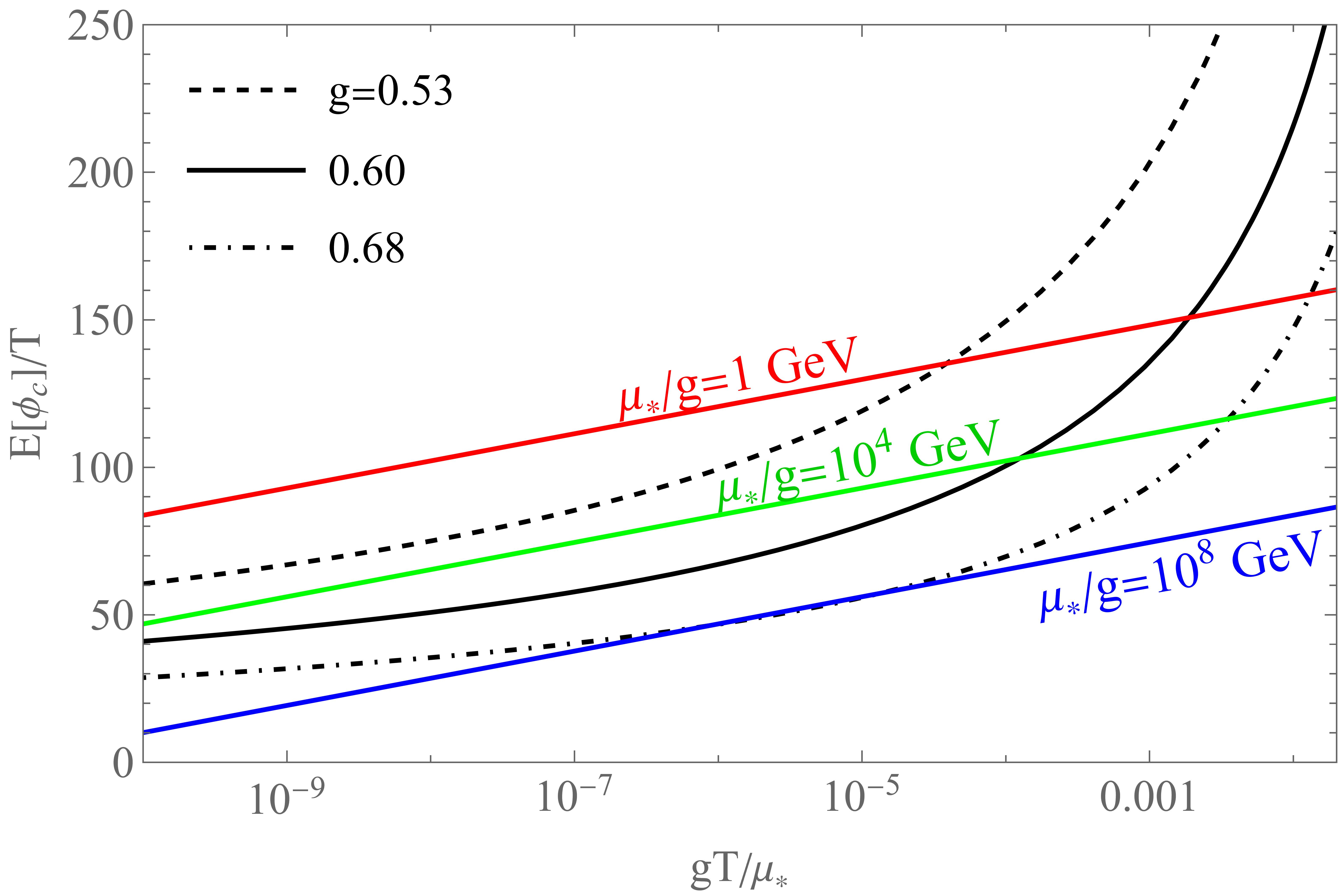
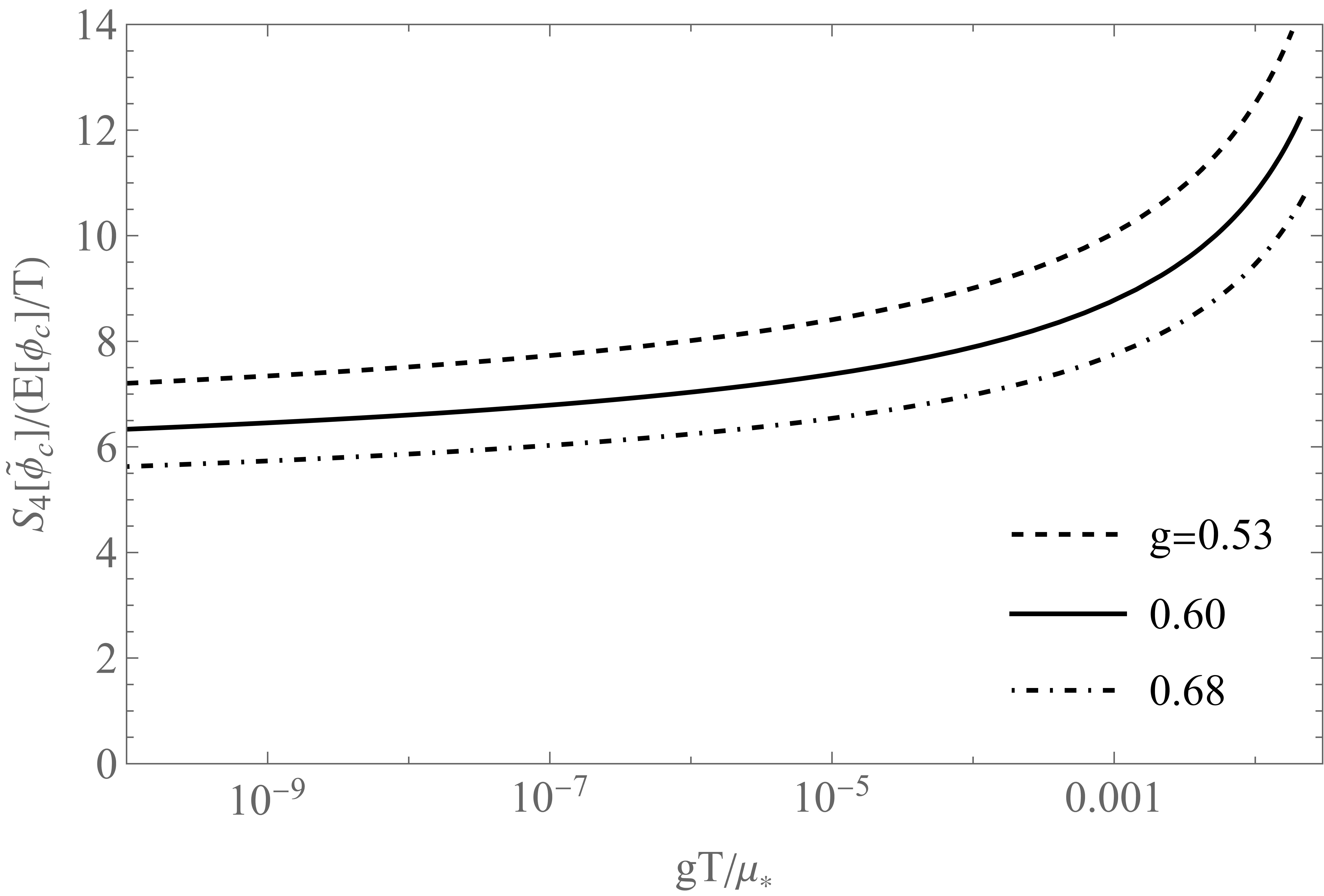
Figure S-2: [Left]: The black curves show $E[\phi_{\mathrm{c}}]/T$ for $g=0.53$ (dashed), $0.60$ (solid), and $0.68$ (dot-dashed) as a function of $gT/\mu_{*}$. The straight lines in different colors show the required values of $E[\phi_{\mathrm{c}}]/T$ for the bubble nucleation rate to match the expansion rate of the universe when $\mu_{*}/g=1\,\mathrm{GeV}$ (red), $10^{4}\,\mathrm{GeV}$ (green), and $10^{8}\,\mathrm{GeV}$ (blue). For given value of $\mu_{*}/g$, the nucleation rate is larger (smaller) than the expansion rate when the curve is below (above) the line. [Right]: Comparison between $E[\phi_{\mathrm{c}}]/T$ and $S_{4}[\tilde{\phi}_{\mathrm{c}}]$ as a function of $gT/\mu_{*}$ for different values of $g$. $S_{4}[\tilde{\phi}_{\mathrm{c}}]$ is always greater than $E[\phi_{\mathrm{c}}]/T$, so the quantum tunnelling contribution to $\Gamma_{\rm n}$ is always exponentially smaller than the thermal one.

It is clear from dimensional analysis that $E[\phi_{\mathrm{c}}]/T$ depends on $T$ and $\mu_{*}$ only through the combination $T/\mu_{*}$. Moreover, $\mu_{*}$ always comes in the combination $\mu_{*}/g$. In Fig. S-2 left, the black curves show $E[\phi_{\mathrm{c}}]/T$ as a function of $gT/\mu_{*}$ for different values of $g$, while the straight lines show the value of the right-hand side of (S.40) as a function of $gT/\mu_{*}$ for different values of $\mu_{*}/g$. For each value of $g$, as we lower the temperature and follow its black curve from top-right to lower-left, when the curve meets the line of given $\mu_{*}/g$, that intersection gives $T_{\rm n}$ for that $\mu_{*}/g$. Since the right-hand side of (S.40) says that the vertical offset of the line increases as $\mu_{*}/g$ decreases, the curve is guaranteed to intersect with the line for any given $g$ if we choose $\mu_{*}/g$ to be sufficiently low. When $\mu_{*}/g$ gets too high, no intersections exist and the bubble nucleation rate would never be large enough to catch up with the expansion rate of the universe. This feature was also pointed out in Ref. [134, 135].

Let us now discuss the quantum tunneling contribution to $\Gamma_{\rm n}$. The exponential part of that contribution is given by $\mathrm{e}^{-S_{4}[\tilde{\phi}_{\mathrm{c}}]}$, where $S_{4}[\phi]$ is given by (S.38) with the replacement $4\pi r^{2}\to 2\pi^{2}r^{3}$ and $\tilde{\phi}_{\mathrm{c}}$ is like $\phi_{\mathrm{c}}$ except that it is from minimizing $S_{4}$ instead. We take the prefactor of the exponential to be $T^{4}$ again by the same argument. In Fig. S-2 right, we see that $S_{4}$ is always greater than $E/T$ so the quantum tunneling contribution is negligible.

To use $\Gamma_{\rm n}$ for the estimation of the PBH abundance described in S2, we need $\Gamma_{\rm n}$ as a function of $t$ rather than $T$. To relate them we use $T(t)=T_{\rm n}\,\mathrm{e}^{-H(t-t_{\rm n})}$. This should be a good approximation as long as the universe is dominated by the vacuum energy, which is the case during the bubble formation period except near the very end of the phase transition when the spacetime is no longer approximately de Sitter.

Once $\Gamma_{\rm n}(t)$ is thus obtained, we calculate $P_{\rm f}(t)$, $P_{\mathrm{PBH}}(t)$, and $n_{\mathrm{PBH}}$ by (S.21), (S.13), and (S.12), respectively. In Fig. S-3, $P_{\rm f}(t)$, $P_{\mathrm{PBH}}(t)$, and the integrand of $n_{\mathrm{PBH}}$ are plotted for the benchmark values of $\mu_{*}=10^{6}\,\mathrm{GeV}$ and three different values of $g$, all with $\kappa=1$ and $\Delta\Omega/4\pi=10^{-3}$.

Fig. 3 in the main text is then obtained by scanning over different values of $g$ and $\mu_{*}$ with various assumptions on $\kappa$ and $\kappa^{2}\Delta\Omega/4\pi$, and trade $\mu_{*}$ for $M_{\mathrm{PBH}}$ or $T_{*\mathrm{max}}$ via (S.24) combined with (S.34). In Fig. S-4, we put some of those result together within a larger plot range, where different values of $g$ are represented by different colors, and for each value of $g$, the solid, dotted, and dashed curves correspond to $\Delta\Omega/4\pi=10^{-2}$, $10^{-3}$ and $10^{-4}$, respectively, all with $\kappa=1$. In particular, we can see in this plot how the sensitivity of $f_{\mathrm{PBH}}$ on the values of $g$ and $\mu_{*}$ rapidly increases as $\Delta\Omega/4\pi$ is reduced, reflecting the fact that $f_{\mathrm{PBH}}$ gets exponentially suppressed as $\Delta\Omega$ decreases. Notice that all the curves terminate as we follow them in the upper-left direction. Those endpoints correspond to the values of $\mu_{*}/g$ beyond which the two intersections of the line with the black curve in Fig. S-2 are too close to each other to have a long enough bubble nucleation period.

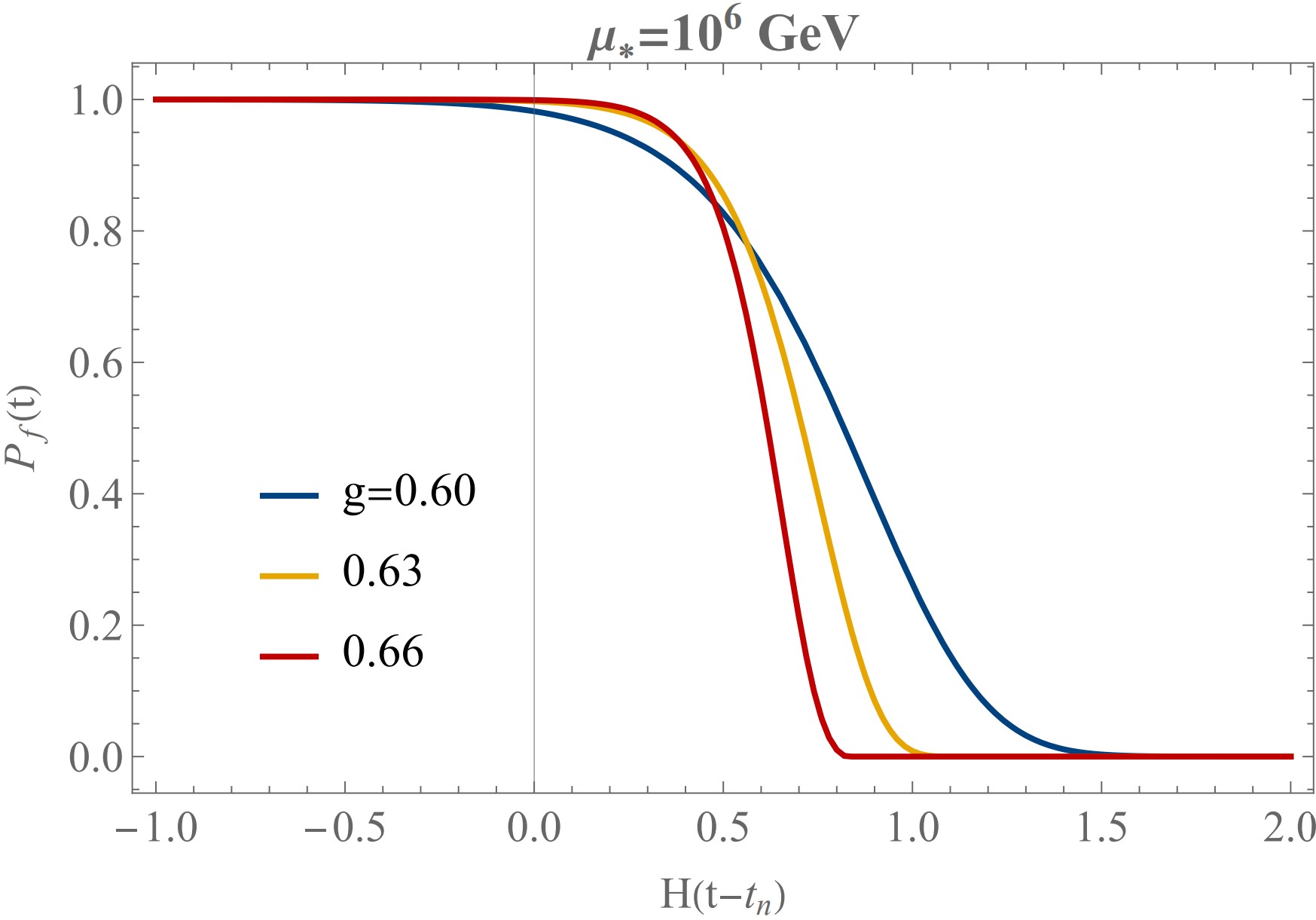
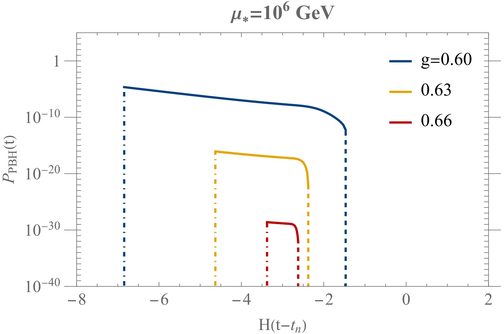
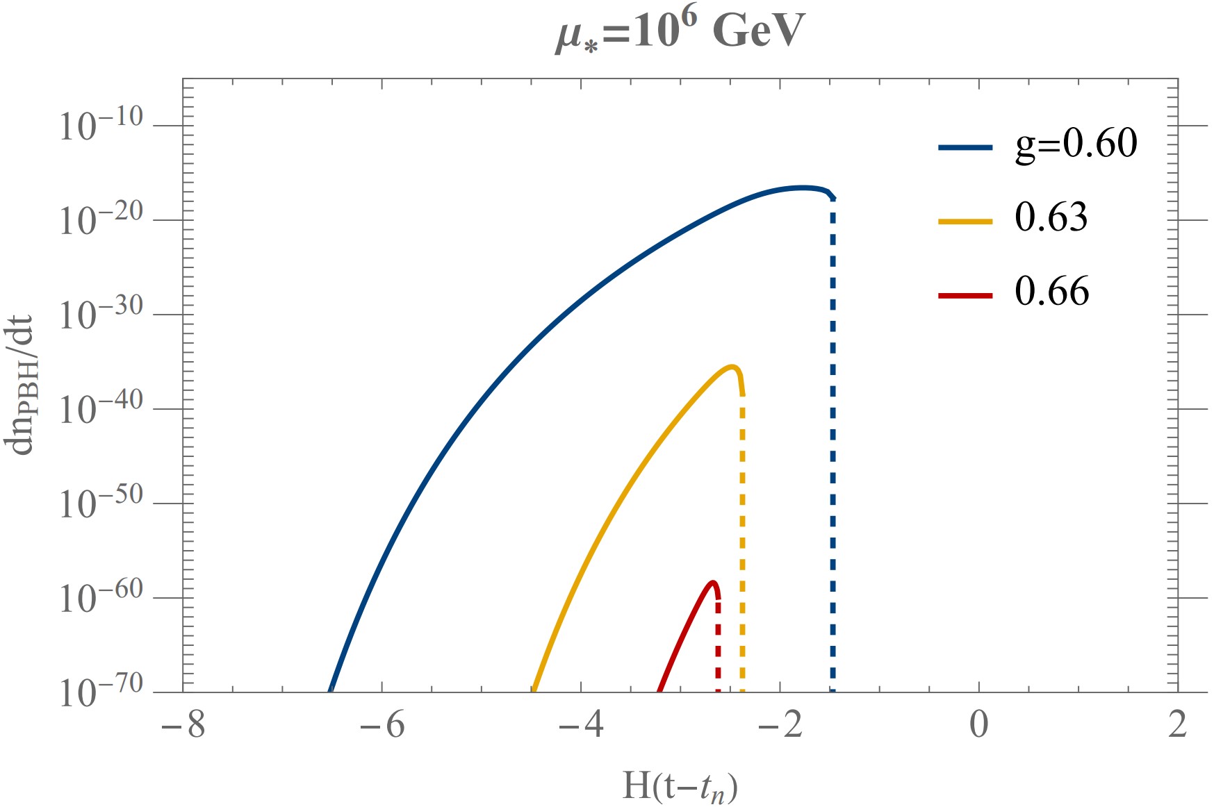
Figure S-3: $P_{\rm f}(t)$ (top), $P_{\mathrm{PBH}}(t)$ (middle), and $\mathrm{d}n_{\mathrm{PBH}}/\mathrm{d}t$ (bottom) as a function of $H(t-t_{\rm n})$ with $\kappa=1$ and $\Delta\Omega/4\pi=10^{-3}$, where $\mathrm{d}n_{\mathrm{PBH}}/\mathrm{d}t$ is the integrand of the right-most expression in (S.12). The dashed lines in the middle and bottom plots indicate the fact that $P_{f}(t_{\rm coll})$ effectively goes to zero in our numerical accuracy. The dot-dashed lines in the middle plot correspond to $t_{\rm c}$.

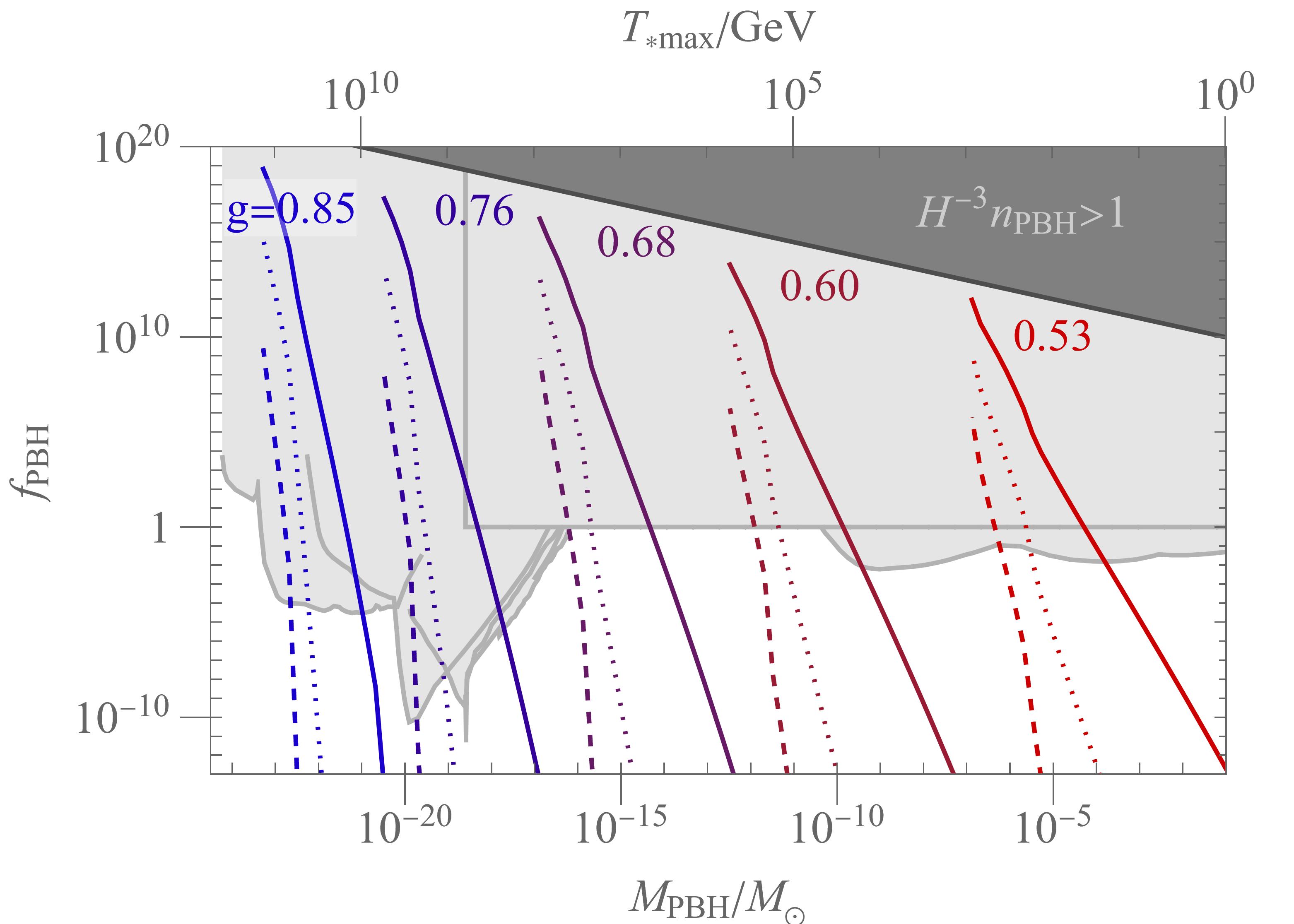
Figure S-4: The PBH abundance $f_{\mathrm{PBH}}$ versus $M_{\mathrm{PBH}}$ (bottom axis) or $T_{*\mathrm{max}}$ (top axis) for $\kappa=1$ and various values of $g$ represented by different colors. For each color, the solid, dotted, and dashed lines correspond to $\Delta\Omega/4\pi=10^{-2}$, $10^{-3}$ and $10^{-4}$, respectively.

References

- [1] D. Chway, T. H. Jung, and C. S. Shin, “Dark matter filtering-out effect during a first-order phase transition,” Phys. Rev. D 101 no. 9, (2020) 095019, arXiv:1912.04238 [hep-ph].
- [2] M. J. Baker, J. Kopp, and A. J. Long, “Filtered Dark Matter at a First Order Phase Transition,” Phys. Rev. Lett. 125 no. 15, (2020) 151102, arXiv:1912.02830 [hep-ph].
- [3] M. Ahmadvand, “Filtered asymmetric dark matter during the Peccei-Quinn phase transition,” arXiv:2108.00958 [hep-ph].
- [4] J.-P. Hong, S. Jung, and K.-P. Xie, “Fermi-ball dark matter from a first-order phase transition,” Phys. Rev. D 102 no. 7, (2020) 075028, arXiv:2008.04430 [hep-ph].
- [5] A. Azatov, M. Vanvlasselaer, and W. Yin, “Dark Matter production from relativistic bubble walls,” JHEP 03 (2021) 288, arXiv:2101.05721 [hep-ph].
- [6] P. Asadi, E. D. Kramer, E. Kuflik, G. W. Ridgway, T. R. Slatyer, and J. Smirnov, “Thermal Squeezeout of Dark Matter,” arXiv:2103.09827 [hep-ph].
- [7] M. E. Shaposhnikov, “Baryon Asymmetry of the Universe in Standard Electroweak Theory,” Nucl. Phys. B 287 (1987) 757–775.
- [8] J. M. Cline, “TASI Lectures on Early Universe Cosmology: Inflation, Baryogenesis and Dark Matter,” PoS TASI2018 (2019) 001, arXiv:1807.08749 [hep-ph].
- [9] E. Hall, T. Konstandin, R. McGehee, H. Murayama, and G. Servant, “Baryogenesis From a Dark First-Order Phase Transition,” JHEP 04 (2020) 042, arXiv:1910.08068 [hep-ph].
- [10] K. Fujikura, K. Harigaya, Y. Nakai, and R. Wang, “Electroweak-like Baryogenesis with New Chiral Matter,” arXiv:2103.05005 [hep-ph].
- [11] J. Arakawa, A. Rajaraman, and T. M. P. Tait, “Annihilogenesis,” arXiv:2109.13941 [hep-ph].
- [12] A. Azatov, M. Vanvlasselaer, and W. Yin, “Baryogenesis via relativistic bubble walls,” JHEP 10 (2021) 043, arXiv:2106.14913 [hep-ph].
- [13] E. Witten, “Cosmic Separation of Phases,” Phys. Rev. D 30 (1984) 272–285.
- [14] C. J. Hogan, “Gravitational radiation from cosmological phase transitions,” Mon. Not. Roy. Astron. Soc. 218 (1986) 629–636.
- [15] A. Kosowsky, M. S. Turner, and R. Watkins, “Gravitational radiation from colliding vacuum bubbles,” Phys. Rev. D 45 (1992) 4514–4535.
- [16] A. Kosowsky and M. S. Turner, “Gravitational radiation from colliding vacuum bubbles: envelope approximation to many bubble collisions,” Phys. Rev. D 47 (1993) 4372–4391, arXiv:astro-ph/9211004.
- [17] M. Kamionkowski, A. Kosowsky, and M. S. Turner, “Gravitational radiation from first order phase transitions,” Phys. Rev. D 49 (1994) 2837–2851, arXiv:astro-ph/9310044.
- [18] J. R. Espinosa, T. Konstandin, J. M. No, and G. Servant, “Energy Budget of Cosmological First-order Phase Transitions,” JCAP 06 (2010) 028, arXiv:1004.4187 [hep-ph].
- [19] C. Caprini et al., “Detecting gravitational waves from cosmological phase transitions with LISA: an update,” JCAP 03 (2020) 024, arXiv:1910.13125 [astro-ph.CO].
- [20] K. Schmitz, “New Sensitivity Curves for Gravitational-Wave Signals from Cosmological Phase Transitions,” JHEP 01 (2021) 097, arXiv:2002.04615 [hep-ph].
- [21] LIGO Scientific Collaboration, G. M. Harry, “Advanced LIGO: The next generation of gravitational wave detectors,” Class. Quant. Grav. 27 (2010) 084006.
- [22] LIGO Scientific Collaboration, J. Aasi et al., “Advanced LIGO,” Class. Quant. Grav. 32 (2015) 074001, arXiv:1411.4547 [gr-qc].
- [23] VIRGO Collaboration, F. Acernese et al., “Advanced Virgo: a second-generation interferometric gravitational wave detector,” Class. Quant. Grav. 32 no. 2, (2015) 024001, arXiv:1408.3978 [gr-qc].
- [24] LISA Collaboration, P. Amaro-Seoane et al., “Laser Interferometer Space Antenna,” arXiv:1702.00786 [astro-ph.IM].
- [25] J. Baker et al., “The Laser Interferometer Space Antenna: Unveiling the Millihertz Gravitational Wave Sky,” arXiv:1907.06482 [astro-ph.IM].
- [26] N. Seto, S. Kawamura, and T. Nakamura, “Possibility of direct measurement of the acceleration of the universe using 0.1-Hz band laser interferometer gravitational wave antenna in space,” Phys. Rev. Lett. 87 (2001) 221103, arXiv:astro-ph/0108011.
- [27] S. Kawamura et al., “The Japanese space gravitational wave antenna: DECIGO,” Class. Quant. Grav. 28 (2011) 094011.
- [28] K. Yagi and N. Seto, “Detector configuration of DECIGO/BBO and identification of cosmological neutron-star binaries,” Phys. Rev. D 83 (2011) 044011, arXiv:1101.3940 [astro-ph.CO]. [Erratum: Phys.Rev.D 95, 109901 (2017)].
- [29] S. Isoyama, H. Nakano, and T. Nakamura, “Multiband Gravitational-Wave Astronomy: Observing binary inspirals with a decihertz detector, B-DECIGO,” PTEP 2018 no. 7, (2018) 073E01, arXiv:1802.06977 [gr-qc].
- [30] J. Crowder and N. J. Cornish, “Beyond LISA: Exploring future gravitational wave missions,” Phys. Rev. D 72 (2005) 083005, arXiv:gr-qc/0506015.
- [31] V. Corbin and N. J. Cornish, “Detecting the cosmic gravitational wave background with the big bang observer,” Class. Quant. Grav. 23 (2006) 2435–2446, arXiv:gr-qc/0512039.
- [32] G. M. Harry, P. Fritschel, D. A. Shaddock, W. Folkner, and E. S. Phinney, “Laser interferometry for the big bang observer,” Class. Quant. Grav. 23 (2006) 4887–4894. [Erratum: Class.Quant.Grav. 23, 7361 (2006)].
- [33] KAGRA Collaboration, K. Somiya, “Detector configuration of KAGRA: The Japanese cryogenic gravitational-wave detector,” Class. Quant. Grav. 29 (2012) 124007, arXiv:1111.7185 [gr-qc].
- [34] KAGRA Collaboration, Y. Aso, Y. Michimura, K. Somiya, M. Ando, O. Miyakawa, T. Sekiguchi, D. Tatsumi, and H. Yamamoto, “Interferometer design of the KAGRA gravitational wave detector,” Phys. Rev. D 88 no. 4, (2013) 043007, arXiv:1306.6747 [gr-qc].
- [35] KAGRA Collaboration, T. Akutsu et al., “KAGRA: 2.5 Generation Interferometric Gravitational Wave Detector,” Nature Astron. 3 no. 1, (2019) 35–40, arXiv:1811.08079 [gr-qc].
- [36] KAGRA Collaboration, T. Akutsu et al., “First cryogenic test operation of underground km-scale gravitational-wave observatory KAGRA,” Class. Quant. Grav. 36 no. 16, (2019) 165008, arXiv:1901.03569 [astro-ph.IM].
- [37] Y. Michimura et al., “Prospects for improving the sensitivity of KAGRA gravitational wave detector,” in 15th Marcel Grossmann Meeting on Recent Developments in Theoretical and Experimental General Relativity, Astrophysics, and Relativistic Field Theories. 6, 2019. arXiv:1906.02866 [gr-qc].
- [38] LIGO Scientific Collaboration, B. P. Abbott et al., “Exploring the Sensitivity of Next Generation Gravitational Wave Detectors,” Class. Quant. Grav. 34 no. 4, (2017) 044001, arXiv:1607.08697 [astro-ph.IM].
- [39] D. Reitze et al., “Cosmic Explorer: The U.S. Contribution to Gravitational-Wave Astronomy beyond LIGO,” Bull. Am. Astron. Soc. 51 no. 7, (2019) 035, arXiv:1907.04833 [astro-ph.IM].
- [40] M. Punturo et al., “The Einstein Telescope: A third-generation gravitational wave observatory,” Class. Quant. Grav. 27 (2010) 194002.
- [41] S. Hild et al., “Sensitivity Studies for Third-Generation Gravitational Wave Observatories,” Class. Quant. Grav. 28 (2011) 094013, arXiv:1012.0908 [gr-qc].
- [42] B. Sathyaprakash et al., “Scientific Objectives of Einstein Telescope,” Class. Quant. Grav. 29 (2012) 124013, arXiv:1206.0331 [gr-qc]. [Erratum: Class.Quant.Grav. 30, 079501 (2013)].
- [43] M. Maggiore et al., “Science Case for the Einstein Telescope,” JCAP 03 (2020) 050, arXiv:1912.02622 [astro-ph.CO].
- [44] S. Burke-Spolaor et al., “The Astrophysics of Nanohertz Gravitational Waves,” Astron. Astrophys. Rev. 27 no. 1, (2019) 5, arXiv:1811.08826 [astro-ph.HE].
- [45] M. A. McLaughlin, “The North American Nanohertz Observatory for Gravitational Waves,” Class. Quant. Grav. 30 (2013) 224008, arXiv:1310.0758 [astro-ph.IM].
- [46] NANOGRAV Collaboration, Z. Arzoumanian et al., “The NANOGrav 11-year Data Set: Pulsar-timing Constraints On The Stochastic Gravitational-wave Background,” Astrophys. J. 859 no. 1, (2018) 47, arXiv:1801.02617 [astro-ph.HE].
- [47] K. Aggarwal et al., “The NANOGrav 11-Year Data Set: Limits on Gravitational Waves from Individual Supermassive Black Hole Binaries,” Astrophys. J. 880 (2019) 2, arXiv:1812.11585 [astro-ph.GA].
- [48] A. Brazier et al., “The NANOGrav Program for Gravitational Waves and Fundamental Physics,” arXiv:1908.05356 [astro-ph.IM].
- [49] R. N. Manchester et al., “The Parkes Pulsar Timing Array Project,” Publ. Astron. Soc. Austral. 30 (2013) 17, arXiv:1210.6130 [astro-ph.IM].
- [50] R. M. Shannon et al., “Gravitational waves from binary supermassive black holes missing in pulsar observations,” Science 349 no. 6255, (2015) 1522–1525, arXiv:1509.07320 [astro-ph.CO].
- [51] M. Kramer and D. J. Champion, “The European Pulsar Timing Array and the Large European Array for Pulsars,” Class. Quant. Grav. 30 (2013) 224009.
- [52] L. Lentati et al., “European Pulsar Timing Array Limits On An Isotropic Stochastic Gravitational-Wave Background,” Mon. Not. Roy. Astron. Soc. 453 no. 3, (2015) 2576–2598, arXiv:1504.03692 [astro-ph.CO].
- [53] S. Babak et al., “European Pulsar Timing Array Limits on Continuous Gravitational Waves from Individual Supermassive Black Hole Binaries,” Mon. Not. Roy. Astron. Soc. 455 no. 2, (2016) 1665–1679, arXiv:1509.02165 [astro-ph.CO].
- [54] G. Hobbs et al., “The international pulsar timing array project: using pulsars as a gravitational wave detector,” Class. Quant. Grav. 27 (2010) 084013, arXiv:0911.5206 [astro-ph.SR].
- [55] R. N. Manchester, “The International Pulsar Timing Array,” Class. Quant. Grav. 30 (2013) 224010, arXiv:1309.7392 [astro-ph.IM].
- [56] J. P. W. Verbiest et al., “The International Pulsar Timing Array: First Data Release,” Mon. Not. Roy. Astron. Soc. 458 no. 2, (2016) 1267–1288, arXiv:1602.03640 [astro-ph.IM].
- [57] J. S. Hazboun, C. M. F. Mingarelli, and K. Lee, “The Second International Pulsar Timing Array Mock Data Challenge,” arXiv:1810.10527 [astro-ph.IM].
- [58] C. L. Carilli and S. Rawlings, “Science with the Square Kilometer Array: Motivation, key science projects, standards and assumptions,” New Astron. Rev. 48 (2004) 979, arXiv:astro-ph/0409274.
- [59] G. Janssen et al., “Gravitational wave astronomy with the SKA,” PoS AASKA14 (2015) 037, arXiv:1501.00127 [astro-ph.IM].
- [60] A. Weltman et al., “Fundamental physics with the Square Kilometre Array,” Publ. Astron. Soc. Austral. 37 (2020) e002, arXiv:1810.02680 [astro-ph.CO].
- [61] B. Carr, K. Kohri, Y. Sendouda, and J. Yokoyama, “Constraints on Primordial Black Holes,” arXiv:2002.12778 [astro-ph.CO].
- [62] B. Carr and F. Kuhnel, “Primordial Black Holes as Dark Matter: Recent Developments,” Ann. Rev. Nucl. Part. Sci. 70 (2020) 355–394, arXiv:2006.02838 [astro-ph.CO].
- [63] G. F. Marani, R. J. Nemiroff, J. P. Norris, K. Hurley, and J. T. Bonnell, “Gravitationally lensed gamma-ray bursts as probes of dark compact objects,” Astrophys. J. Lett. 512 (1999) L13, arXiv:astro-ph/9810391.
- [64] R. J. Nemiroff, G. F. Marani, J. P. Norris, and J. T. Bonnell, “Limits on the cosmological abundance of supermassive compact objects from a millilensing search in gamma-ray burst data,” Phys. Rev. Lett. 86 (2001) 580, arXiv:astro-ph/0101488.
- [65] A. Barnacka, J. F. Glicenstein, and R. Moderski, “New constraints on primordial black holes abundance from femtolensing of gamma-ray bursts,” Phys. Rev. D 86 (2012) 043001, arXiv:1204.2056 [astro-ph.CO].
- [66] A. Katz, J. Kopp, S. Sibiryakov, and W. Xue, “Femtolensing by Dark Matter Revisited,” JCAP 12 (2018) 005, arXiv:1807.11495 [astro-ph.CO].
- [67] K. Griest, A. M. Cieplak, and M. J. Lehner, “New Limits on Primordial Black Hole Dark Matter from an Analysis of Kepler Source Microlensing Data,” Phys. Rev. Lett. 111 no. 18, (2013) 181302.
- [68] K. Griest, A. M. Cieplak, and M. J. Lehner, “Experimental Limits on Primordial Black Hole Dark Matter from the First 2 yr of Kepler Data,” Astrophys. J. 786 no. 2, (2014) 158, arXiv:1307.5798 [astro-ph.CO].
- [69] H. Niikura et al., “Microlensing constraints on primordial black holes with Subaru/HSC Andromeda observations,” Nature Astron. 3 no. 6, (2019) 524–534, arXiv:1701.02151 [astro-ph.CO].
- [70] B. Paczynski, “Gravitational microlensing by the galactic halo,” Astrophys. J. 304 (1986) 1–5.
- [71] C. Hamadache et al., “Galactic bulge microlensing optical depth from eros-2,” Astron. Astrophys. 454 (2006) 185–199, arXiv:astro-ph/0601510.
- [72] L. Wyrzykowski et al., “The OGLE View of Microlensing towards the Magellanic Clouds. I. A Trickle of Events in the OGLE-II LMC data,” Mon. Not. Roy. Astron. Soc. 397 (2009) 1228–1242, arXiv:0905.2044 [astro-ph.GA].
- [73] S. Calchi Novati, L. Mancini, G. Scarpetta, and L. Wyrzykowski, “LMC self lensing for OGLE-II microlensing observations,” Mon. Not. Roy. Astron. Soc. 400 (2009) 1625, arXiv:0908.3836 [astro-ph.GA].
- [74] L. Wyrzykowski et al., “The OGLE View of Microlensing towards the Magellanic Clouds. II. OGLE-II SMC data,” Mon. Not. Roy. Astron. Soc. 407 (2010) 189–200, arXiv:1004.5247 [astro-ph.GA].
- [75] L. Wyrzykowski et al., “The OGLE View of Microlensing towards the Magellanic Clouds. III. Ruling out sub-solar MACHOs with the OGLE-III LMC data,” Mon. Not. Roy. Astron. Soc. 413 (2011) 493, arXiv:1012.1154 [astro-ph.GA].
- [76] L. Wyrzykowski et al., “The OGLE View of Microlensing towards the Magellanic Clouds. IV. OGLE-III SMC Data and Final Conclusions on MACHOs,” Mon. Not. Roy. Astron. Soc. 416 (2011) 2949, arXiv:1106.2925 [astro-ph.GA].
- [77] H. Niikura, M. Takada, S. Yokoyama, T. Sumi, and S. Masaki, “Constraints on Earth-mass primordial black holes from OGLE 5-year microlensing events,” Phys. Rev. D 99 no. 8, (2019) 083503, arXiv:1901.07120 [astro-ph.CO].
- [78] M. Zumalacarregui and U. Seljak, “Limits on stellar-mass compact objects as dark matter from gravitational lensing of type Ia supernovae,” Phys. Rev. Lett. 121 no. 14, (2018) 141101, arXiv:1712.02240 [astro-ph.CO].
- [79] J. Garcia-Bellido, S. Clesse, and P. Fleury, “Primordial black holes survive SN lensing constraints,” Phys. Dark Univ. 20 (2018) 95–100, arXiv:1712.06574 [astro-ph.CO].
- [80] D. N. Page and S. W. Hawking, “Gamma rays from primordial black holes,” Astrophys. J. 206 (1976) 1–7.
- [81] B. J. Carr, K. Kohri, Y. Sendouda, and J. Yokoyama, “New cosmological constraints on primordial black holes,” Phys. Rev. D 81 (2010) 104019, arXiv:0912.5297 [astro-ph.CO].
- [82] B. J. Carr, K. Kohri, Y. Sendouda, and J. Yokoyama, “Constraints on primordial black holes from the Galactic gamma-ray background,” Phys. Rev. D 94 no. 4, (2016) 044029, arXiv:1604.05349 [astro-ph.CO].
- [83] M. Boudaud and M. Cirelli, “Voyager 1 Further Constrain Primordial Black Holes as Dark Matter,” Phys. Rev. Lett. 122 no. 4, (2019) 041104, arXiv:1807.03075 [astro-ph.HE].
- [84] W. DeRocco and P. W. Graham, “Constraining Primordial Black Hole Abundance with the Galactic 511 keV Line,” Phys. Rev. Lett. 123 no. 25, (2019) 251102, arXiv:1906.07740 [astro-ph.CO].
- [85] R. Laha, “Primordial Black Holes as a Dark Matter Candidate Are Severely Constrained by the Galactic Center 511 keV -Ray Line,” Phys. Rev. Lett. 123 no. 25, (2019) 251101, arXiv:1906.09994 [astro-ph.HE].
- [86] B. Dasgupta, R. Laha, and A. Ray, “Neutrino and positron constraints on spinning primordial black hole dark matter,” Phys. Rev. Lett. 125 no. 10, (2020) 101101, arXiv:1912.01014 [hep-ph].
- [87] R. Laha, J. B. Muñoz, and T. R. Slatyer, “INTEGRAL constraints on primordial black holes and particle dark matter,” Phys. Rev. D 101 no. 12, (2020) 123514, arXiv:2004.00627 [astro-ph.CO].
- [88] M. H. Chan and C. M. Lee, “Constraining Primordial Black Hole Fraction at the Galactic Centre using radio observational data,” Mon. Not. Roy. Astron. Soc. 497 no. 1, (2020) 1212–1216, arXiv:2007.05677 [astro-ph.HE].
- [89] K. M. Belotsky and A. A. Kirillov, “Primordial black holes with mass g and reionization of the Universe,” JCAP 01 (2015) 041, arXiv:1409.8601 [astro-ph.CO].
- [90] H. Kim, “A constraint on light primordial black holes from the interstellar medium temperature,” arXiv:2007.07739 [hep-ph].
- [91] S. W. Hawking, I. G. Moss, and J. M. Stewart, “Bubble Collisions in the Very Early Universe,” Phys. Rev. D 26 (1982) 2681.
- [92] K. Sato, M. Sasaki, H. Kodama, and K.-i. Maeda, “Creation of Wormholes by First Order Phase Transition of a Vacuum in the Early Universe,” Prog. Theor. Phys. 65 (1981) 1443.
- [93] K.-i. Maeda, K. Sato, M. Sasaki, and H. Kodama, “Creation of De Sitter-schwarzschild Wormholes by a Cosmological First Order Phase Transition,” Phys. Lett. B 108 (1982) 98–102.
- [94] H. Kodama, M. Sasaki, and K. Sato, “Abundance of Primordial Holes Produced by Cosmological First Order Phase Transition,” Prog. Theor. Phys. 68 (1982) 1979.
- [95] L. J. Hall and S. Hsu, “Cosmological Production of Black Holes,” Phys. Rev. Lett. 64 (1990) 2848–2851.
- [96] A. Kusenko, M. Sasaki, S. Sugiyama, M. Takada, V. Takhistov, and E. Vitagliano, “Exploring Primordial Black Holes from the Multiverse with Optical Telescopes,” Phys. Rev. Lett. 125 (2020) 181304, arXiv:2001.09160 [astro-ph.CO].
- [97] M. Y. Khlopov, R. V. Konoplich, S. G. Rubin, and A. S. Sakharov, “First order phase transitions as a source of black holes in the early universe,” Grav. Cosmol. 2 (1999) S1, arXiv:hep-ph/9912422.
- [98] M. Lewicki and V. Vaskonen, “On bubble collisions in strongly supercooled phase transitions,” Phys. Dark Univ. 30 (2020) 100672, arXiv:1912.00997 [astro-ph.CO].
- [99] C. Gross, G. Landini, A. Strumia, and D. Teresi, “Dark Matter as dark dwarfs and other macroscopic objects: multiverse relics?,” JHEP 09 (2021) 033, arXiv:2105.02840 [hep-ph].
- [100] M. J. Baker, M. Breitbach, J. Kopp, and L. Mittnacht, “Primordial Black Holes from First-Order Cosmological Phase Transitions,” arXiv:2105.07481 [astro-ph.CO].
- [101] K. Kawana and K.-P. Xie, “Primordial black holes from a cosmic phase transition: The collapse of Fermi-balls,” Phys. Lett. B 824 (2022) 136791, arXiv:2106.00111 [astro-ph.CO].
- [102] M. J. Baker, M. Breitbach, J. Kopp, and L. Mittnacht, “Detailed Calculation of Primordial Black Hole Formation During First-Order Cosmological Phase Transitions,” arXiv:2110.00005 [astro-ph.CO].
- [103] J. Liu, L. Bian, R.-G. Cai, Z.-K. Guo, and S.-J. Wang, “Primordial black hole production during first-order phase transitions,” Phys. Rev. D 105 no. 2, (2022) L021303, arXiv:2106.05637 [astro-ph.CO].
- [104] K. Hashino, S. Kanemura, and T. Takahashi, “Primordial black holes as a probe of strongly first-order electroweak phase transition,” Phys. Lett. B 833 (2022) 137261, arXiv:2111.13099 [hep-ph].
- [105] P. Huang and K.-P. Xie, “Primordial black holes from an electroweak phase transition,” Phys. Rev. D 105 no. 11, (2022) 115033, arXiv:2201.07243 [hep-ph].
- [106] V. De Luca, G. Franciolini, and A. Riotto, “Heavy Primordial Black Holes from Strongly Clustered Light Black Holes,” Phys. Rev. Lett. 130 no. 17, (2023) 171401, arXiv:2210.14171 [astro-ph.CO].
- [107] K. Kawana, T. Kim, and P. Lu, “PBH formation from overdensities in delayed vacuum transitions,” Phys. Rev. D 108 no. 10, (2023) 103531, arXiv:2212.14037 [astro-ph.CO].
- [108] M. Lewicki, P. Toczek, and V. Vaskonen, “Primordial black holes from strong first-order phase transitions,” JHEP 09 (2023) 092, arXiv:2305.04924 [astro-ph.CO].
- [109] Y. Gouttenoire and T. Volansky, “Primordial Black Holes from Supercooled Phase Transitions,” arXiv:2305.04942 [hep-ph].
- [110] R. Jinno, J. Kume, and M. Yamada, “Super-slow phase transition catalyzed by BHs and the birth of baby BHs,” arXiv:2310.06901 [hep-ph].
- [111] K. S. Thorne, “Nonspherical gravitational collapse: A short review,” in Magic Without Magic: John Archibald Wheeler, J. Klauder, ed., p. 231. Freeman, San Francisco, 1972.
- [112] W. E. East and F. Pretorius, “Ultrarelativistic black hole formation,” Phys. Rev. Lett. 110 no. 10, (2013) 101101, arXiv:1210.0443 [gr-qc].
- [113] W.-Y. Ai, “Logarithmically divergent friction on ultrarelativistic bubble walls,” arXiv:2308.10679 [hep-ph].
- [114] D. Bodeker and G. D. Moore, “Electroweak Bubble Wall Speed Limit,” JCAP 05 (2017) 025, arXiv:1703.08215 [hep-ph].
- [115] S. Höche, J. Kozaczuk, A. J. Long, J. Turner, and Y. Wang, “Towards an all-orders calculation of the electroweak bubble wall velocity,” JCAP 03 (2021) 009, arXiv:2007.10343 [hep-ph].
- [116] Y. Gouttenoire, R. Jinno, and F. Sala, “Friction pressure on relativistic bubble walls,” JHEP 05 (2022) 004, arXiv:2112.07686 [hep-ph].
- [117] A. Azatov, G. Barni, R. Petrossian-Byrne, and M. Vanvlasselaer, “Quantisation Across Bubble Walls and Friction,” arXiv:2310.06972 [hep-ph].
- [118] M. S. Turner, E. J. Weinberg, and L. M. Widrow, “Bubble nucleation in first order inflation and other cosmological phase transitions,” Phys. Rev. D 46 (1992) 2384–2403.
- [119] S. W. Hawking, “Black hole explosions,” Nature 248 (1974) 30–31.
- [120] S. W. Hawking, “Particle Creation by Black Holes,” Commun. Math. Phys. 43 (1975) 199–220. [Erratum: Commun.Math.Phys. 46, 206 (1976)].
- [121] A. Coogan, L. Morrison, and S. Profumo, “Direct Detection of Hawking Radiation from Asteroid-Mass Primordial Black Holes,” Phys. Rev. Lett. 126 no. 17, (2021) 171101, arXiv:2010.04797 [astro-ph.CO].
- [122] A. Ray, R. Laha, J. B. Muñoz, and R. Caputo, “Near future MeV telescopes can discover asteroid-mass primordial black hole dark matter,” Phys. Rev. D 104 no. 2, (2021) 023516, arXiv:2102.06714 [astro-ph.CO].
- [123] D. Ghosh, D. Sachdeva, and P. Singh, “Future Constraints on Primordial Black Holes from XGIS-THESEUS,” arXiv:2110.03333 [astro-ph.CO].
- [124] S. D. Hunter et al., “A Pair Production Telescope for Medium-Energy Gamma-Ray Polarimetry,” Astropart. Phys. 59 (2014) 18–28, arXiv:1311.2059 [astro-ph.IM].
- [125] AMEGO Collaboration, R. Caputo et al., “All-sky Medium Energy Gamma-ray Observatory: Exploring the Extreme Multimessenger Universe,” arXiv:1907.07558 [astro-ph.IM].
- [126] e-ASTROGAM Collaboration, M. Tavani et al., “Science with e-ASTROGAM: A space mission for MeV–GeV gamma-ray astrophysics,” JHEAp 19 (2018) 1–106, arXiv:1711.01265 [astro-ph.HE].
- [127] A. Moiseev, S. Profumo, A. Coogan, and L. Morrison, “Snowmass 2021 Letter of Interest: Searching for Dark Matter and New Physics with GECCO, 2020,”. https://www.snowmass21.org/docs/files/summaries/CF/SNOWMASS21-CF3_CF1_Stefano_Profumo-007.pdf.
- [128] T. Dzhatdoev and E. Podlesnyi, “Massive Argon Space Telescope (MAST): A concept of heavy time projection chamber for -ray astronomy in the 100 MeV–1 TeV energy range,” Astropart. Phys. 112 (2019) 1–7, arXiv:1902.01491 [astro-ph.HE].
- [129] X. Wu, M. Su, A. Bravar, J. Chang, Y. Fan, M. Pohl, and R. Walter, “PANGU: A High Resolution Gamma-ray Space Telescope,” Proc. SPIE Int. Soc. Opt. Eng. 9144 (2014) 91440F, arXiv:1407.0710 [astro-ph.IM].
- [130] T. Aramaki, P. Hansson Adrian, G. Karagiorgi, and H. Odaka, “Dual MeV Gamma-Ray and Dark Matter Observatory - GRAMS Project,” Astropart. Phys. 114 (2020) 107–114, arXiv:1901.03430 [astro-ph.HE].
- [131] C. Labanti et al., “The X/Gamma-ray Imaging Spectrometer (XGIS) on-board THESEUS: design, main characteristics, and concept of operation,” in SPIE Astronomical Telescopes + Instrumentation 2020. 2, 2021. arXiv:2102.08701 [astro-ph.IM].
- [132] THESEUS Consortium Collaboration, L. Amati et al., “The THESEUS space mission: science goals, requirements and mission concept,” arXiv:2104.09531 [astro-ph.IM].
- [133] C. L. Wainwright, “CosmoTransitions: Computing Cosmological Phase Transition Temperatures and Bubble Profiles with Multiple Fields,” Comput. Phys. Commun. 183 (2012) 2006–2013, arXiv:1109.4189 [hep-ph].
- [134] J. Ellis, M. Lewicki, and J. M. No, “On the Maximal Strength of a First-Order Electroweak Phase Transition and its Gravitational Wave Signal,” JCAP 04 (2019) 003, arXiv:1809.08242 [hep-ph].
- [135] M. Lewicki, O. Pujolàs, and V. Vaskonen, “Escape from supercooling with or without bubbles: gravitational wave signatures,” Eur. Phys. J. C 81 no. 9, (2021) 857, arXiv:2106.09706 [astro-ph.CO].