Fast emulation of quantum three-body scattering

Abstract

We develop a class of emulators for solving quantum three-body scattering problems. They are based on combining the variational method for scattering observables and the recently proposed eigenvector continuation concept. The emulators are first trained by the exact scattering solutions of the governing Hamiltonian at a small number of points in its parameter space, and then employed to make interpolations and extrapolations in that space. Through a schematic nuclear-physics model with finite-range two and three-body interactions, we demonstrate the emulators to be extremely accurate and efficient. The computing time for emulation is on the scale of milliseconds (on a laptop), with relative errors ranging from $10^{-13}$ to $10^{-4}$ depending on the case. The emulators also require little memory. We argue that these emulators can be generalized to even more challenging scattering problems. Furthermore, this general strategy may be applicable for building the same type of emulators in other fields, wherever variational methods can be developed for evaluating physical models.

I Introduction

Methods to solve quantum three-body scattering problems, i.e., the Faddeev approach Glöckle (1983); Gloeckle et al. (1996); Nielsen et al. (2001); Deltuva et al. (2014), are well developed but are complex and computationally expensive in terms of both time and memory costs. This is a severe barrier to applications that require many evaluations in the parameter space of the governing Hamiltonian $H$, such as Bayesian uncertainty quantification. An alternative to direct solutions of the three-body equations for each parameter set is to use emulators. These are models trained on the full solutions for a small number of parameter sets that provide predictions elsewhere in the parameter space for a small fraction of the computational time and memory requirements. In this work, we demonstrate effective emulation of three-body scattering by generalizing the eigenvector continuation (EC) method originally proposed for bound-state calculations Frame (2019).

Emulators based on Gaussian processes (GP) MacKay (1998); Rasmussen and Williams (2006) and on neural networks (e.g., Bogojeski et al. (2020); Breen et al. (2020)) have been widely used in physics and other fields. A different type of emulator is based on EC applied to variational calculations. In short, the eigenvectors from the training solutions can be used as an extremely effective basis for variational estimates. In nuclear physics, fast and accurate EC emulators have been developed recently for few- and many-body ground states König et al. (2020); Ekström and Hagen (2019); Wesolowski et al. (2021), excited states Franzke et al. (2021), and transitions Wesolowski et al. (2021); for shell-model calculations Yoshida and Shimizu (2021); and, of particular relevance here, for two-body scattering Furnstahl et al. (2020); Melendez et al. (2021); Drischler et al. (2021). They are particularly efficacious for Bayesian statistical analyses, where extensive sampling in the parameter space is typically needed for parameter estimation, propagation of errors to observables, and experimental design.

An extension of EC emulators to three-body scattering would have broad impact. Potential applications in nuclear physics include parameter estimation for chiral effective field theory Epelbaum et al. (2009); Hebeler (2021)—which is the foundation for modern ab initio calculations—and for phenomenological reaction models needed in analyzing data from rare isotope facilities King et al. (2019); analyzing Lattice QCD simulations of three-nucleon or hadron systems Eliyahu et al. (2020); and facilitating the generalization of a new approach for ab initio scattering calculations Zhang et al. (2020a) to three-cluster systems.

Considered in a even broader context, three-body scattering, and particle scattering from a two-particle bound system in particular, represents a process of one particle probing a compound target. The EC emulators with proper generalization for the compound systems could expedite scattering data analyses and the extraction of the structure information for a wide range of targets. This study is the first step towards constructing EC emulators for general reactions including inelastic and breakup processes. More generally, as discussed in the end of this paper, a complete set of EC emulators would enable a new type of workflow in nuclear physics and beyond.

The variational method for quantum ground states is well-known from introductory courses in quantum mechanics. Less familiar are the variational approaches for scattering observables due to Kohn, Schwinger, and others. The Kohn variational principle (KVP) is based on a stationary functional at fixed energy. It does not provide bounds to S-matrix elements but nevertheless has been effectively applied, particular in atomic physics Nesbet (1980). As with any variational approach, the key to success is choosing a good ansatz or basis for the trial function. The secret of EC is that the subspace covered by the wave functions of interest when sweeping through the parameters is a much smaller space than the full Hilbert space of wave functions. This subspace is well-spanned by a small subset of these wave functions (the training points), which comprise the EC trial function. The effectiveness of EC emulation applying the KVP has been demonstrated for two-body scattering observables Furnstahl et al. (2020), and for $R$ matrix theory calculations of fusion observables Bai and Ren (2021).

Here we extend the EC with KVP to three-body scattering and give a proof-of-principle demonstration for spin-zero bosons with separable potentials. The relative errors for emulating $S$ matrix elements and the computing time and memory costs for each emulation are summarized in Table 1 for three different cases. The time cost is generally milliseconds on a laptop, and the memory costs are tiny. When the Hamiltonian’s parametric dependence can be factorized from individual potential operators (the “linear” case in the table), e.g., with linear coupling strengths for the potential, the EC emulator works at its full advantage with an extremely small error. The accuracy deteriorates when varying the interaction operators (“nonlinear-1”), e.g., the ranges of interactions, and varying the structure of the subclusters (“nonlinear-2”), but they are still far better than needed in most nuclear physics applications. For emulating more complicated realistic calculations, the costs and accuracy would be similar. This is elaborated further in Sec. V.

In comparison, solving three-body scattering Faddeev equations is computationally expensive. For example, nucleon-deuteron ($N$-$d$) scattering is generally computed using supercomputers Gloeckle et al. (1996); Witala and Gloeckle (2012); Pomerantsev et al. (2016).. Performing such calculations many thousands or even millions of times, as required in (Bayesian) data analysis and experimental design, is so expensive that no such calculation has appeared to date. The emulators developed here can solve this bottleneck issue.

EC emulators	$S$ Relative error	Time	Memory
linear	$10^{-14}\sim 10^{-13}$	ms	$<$ MB
nonlinear-1	$10^{-6}\sim 10^{-5}$	ms	MB
nonlinear-2	$10^{-4}$	ms	10s MB

Table 1: A summary of the accuracy, and time and memory costs of the emulators that we have developed for varying the interaction parameters. The values listed here are representative and reflect their means for test points in the parameter space and for the typical numbers of trainings we employed in this work. Details can be found in Sec. IV.

In Sec. II, we elaborate on the formulation of emulators combining EC and KVP. The necessary elements of three-body scattering and the KVP are reviewed in Sec. III and exemplary results for the EC emulators are shown in Sec. IV. Our summary and outlook is in Sec. V. Additional details on conventions, three-body scattering wave functions, and EC emulators are given in the appendices and Supplementary Material (SM). The self-contained set of codes that can be used to generate our results will be made public BUQEYE collaboration .

II Variational-plus-EC emulation

The general emulator strategy we use starts with a functional $\mathcal{F}_{\bm{\theta}}[\Psi]$ characterizing the physical system of interest. Here $\Psi$ specifies a state of the system and $\bm{\theta}$ is a vector of parameters to be varied for emulation. For example, $\bm{\theta}$ could determine the Hamiltonian and $\Psi$ could be the ground-state eigenvector or a scattering state solution at a specified energy. The functional is stationary at the exact $\Psi$, but not necessarily an extremum. The insight from EC, or the reduced basis method Rheinboldt (1993); Chen et al. (2017) more generally, is in constructing a trial basis for $\Psi$ that enables the relevant physical observables to be calculated more efficiently for many instances of $\bm{\theta}$ than possible by direct solution.

That is, EC suggests that a very effective way of choosing a variational trial function $\Psi_{t}$ for solving the problem at $\bm{\theta}$ is to use

$$\Psi_{t}=\sum_{i=1}^{N_{b}}c_{i}\,\Psi^{(i)},$$ (2)

where the $\Psi^{(i)}$ are exact solutions determined at $N_{b}$ parameter vectors $\bm{\theta}_{i}$ for $i=1,2,...,N_{b}$. If there are constraints on the trial state in the form $\mathcal{G}[\Psi_{t}]=0$, they can be enforced with the Lagrange multiplier method; the final functional we need to work with is $\mathcal{F}_{\bm{\theta}}[\Psi_{t}]+\lambda_{\text{L}}\mathcal{G}[\Psi_{t}]$. To find the stationary point with $\Psi_{t}$, we need to find $c_{i}$ and $\lambda_{\text{L}}$ that make the first derivatives zero, i.e.,

$$\frac{\partial\bigl{(}\mathcal{F}_{\bm{\theta}}[\Psi_{t}]+\lambda_{\text{L}}\mathcal{G}[\Psi_{t}]\bigr{)}}{\partial c_{i}} =0,$$ (3)

$$\mathcal{G}[\Psi_{t}] =0.$$ (4)

Knowing the $c_{i}$, we can compute $\Psi_{t}$ and evaluate the functional to get estimates of quantities of interest, such as the energy. The efficiency of EC originates from $N_{b}$ being a small number in practice to get high accuracy, much smaller than needed for a typical basis spanning the full Hilbert space.

II.1 Many-body bound state emulators

In few- and many-body bound-state calculations, the functional for estimating the ground-state energy is

$$\mathcal{F}_{\bm{\theta}}[\Psi_{t}] =\langle\Psi_{t}|H(\bm{\theta})|\Psi_{t}\rangle,$$ (5)

$$\mathcal{G}[\Psi_{t}] =\langle\Psi_{t}|\Psi_{t}\rangle-1,$$ (6)

The resulting equation for evaluating the EC emulator is a $N_{b}$-dimensional generalized eigenvalue problem, which can be solved extremely fast and with little memory for small $N_{b}$. In the previous bound-state emulator studies König et al. (2020); Ekström and Hagen (2019) treating chiral potentials and their to-be-fitted low-energy constants (LECs), the $\bm{\theta}$ dependence of the potential term in $H$ is linear, i.e., $V(\bm{\theta})=\sum_{n=1}^{N}\theta_{n}\,O_{n}$. The coefficients of the resulted linear equations depend on $\langle\Psi^{(i)}|O_{n}|\Psi^{(j)}\rangle$ and $\langle\Psi^{(i)}|\Psi^{(j)}\rangle$. These matrix elements, even though possibly costly to evaluate, can be computed and saved at the emulator-training stage and tabulated for use in the emulating stage. The resulting emulators are extremely fast and accurate Frame et al. (2018); König et al. (2020); Ekström and Hagen (2019).

II.2 Two-body scattering emulator

For the two-body scattering calculation, the KVP functional for estimating the $S$ matrix takes the form (and similarly for the $T$ or $K$ matrices),

$$\mathcal{F}_{\bm{\theta}}[\Psi_{t}] =S_{t}-\frac{i}{\mathcal{C}}\langle\Psi_{t}|E-H(\bm{\theta})|\Psi_{t}\rangle.$$ (7)

$S_{t}$ is the $S$-matrix of the scattering wave function $\Psi_{t}$, which can be inferred from the asymptotic behavior of $\Psi_{t}$ at large separation; i.e., in a particular partial wave $\ell$ channel,

$$\Psi_{t}(r)\underset{r\rightarrow\infty}{\longrightarrow}\frac{1}{\sqrt{v}}\bigl{(}-\hat{h}_{\ell}^{(-)}(pr)+S_{t}\,\hat{h}_{\ell}^{(+)}(pr)\bigr{)}\;.$$ (8)

$\hat{h}_{\ell}^{(\pm)}$ are the outgoing and incoming spherical waves Descouvemont (2016), $v$ is the relative velocity, and the coefficient $\mathcal{C}=1$ for this particular normalization of the scattering wave function. In this case

$$\mathcal{G}[\Psi_{t}]=\sum_{i=1}^{N_{b}}c_{i}-1.$$ (9)

The functional with the EC trial wave function becomes

$$\mathcal{F}_{\bm{\theta}} =\sum_{i=1}^{N_{b}}c_{i}S^{(i)}-\sum_{i,j=1}^{N_{b}}c_{i}c_{j}\delta\tilde{U}_{i,j},$$ (10)

$$\delta{U}_{i,j} \equiv\frac{1}{2i\mathcal{C}}\langle\Psi^{(i)}|H-E|\Psi^{(j)}\rangle.$$ (11)

$$\delta\tilde{U}_{i,j} =\delta{U}_{i,j}+\delta{U}_{j,i}.$$ (12)

$S^{(i)}$ is the $S$ matrix at the $i$th training point. We then get a set of linear equations for finding the stationary point of the functional:

$$2\sum_{j=1}^{N_{b}}\delta\tilde{U}_{i,j}c_{j}+\lambda_{\text{L}} =S^{(i)}\ \text{with}\ i=1,,,N_{b}$$ (13)

$$\sum_{i=1}^{N_{b}}c_{i} =1,$$ (14)

which can be directly solved using a linear equation solver. The equations can become ill-conditioned as $N_{b}$ increases; here we precondition them using nugget regularization Furnstahl et al. (2020).

As with the bound-state emulators, if the $\bm{\theta}$ dependence in $H(\bm{\theta})$ is factorized from individual potential operators, i.e., $V(\bm{\theta})=\sum_{n=1}^{N}\theta_{n}O_{n}$, the $\langle\Psi^{(i)}|O_{n}|\Psi^{(j)}\rangle$ pieces in $\delta{U}_{i,j}$ can be computed and stored at the training stage and directly reused when emulating. These emulators can be extremely fast and needs little memory, because the only cost is solving the low-dimension linear equations. In Sec. IV we explore ways to construct efficient EC emulators when the parameter factorization condition is not met.

III Three-body scattering

III.1 Exact solution of Faddeev scattering equations

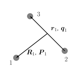
Figure 1: A schematic layout of a 3-body system with a particular choice of coordinate and momentum variables for describing the internal dynamics.

There are three equivalent sets of kinetic variables describing a three-body system. In Fig. 1, we consider particles ‘2’ and ‘3’ a dimer system and particle ‘1’ a spectator. The variables $\bm{r}_{1}$ and $\bm{q}_{1}$ are the relative coordinate and momentum vector between ‘2’ and ‘3’, while $\bm{R}_{1}$ and $\bm{P}_{1}$ are those between the spectator and the center-of-mass (CM) of the dimer. The other two sets of coordinates arise from permutations of the particle indices. See Appendix A for further details. The notation conventions in Ref. Glöckle (1983) will be followed here generally, except that the assignments of momentum variables are different: $P\leftrightarrow q_{\text{Ref.\,\cite[cite]{\@@bibref{Authors Phrase1YearPhrase2}{Glockle:1983}{\@@citephrase{(}}{\@@citephrase{)}}}}}$, $q\leftrightarrow p_{\text{Ref.\,\cite[cite]{\@@bibref{Authors Phrase1YearPhrase2}{Glockle:1983}{\@@citephrase{(}}{\@@citephrase{)}}}}}$.

In this work, we focus on the case where there is a bound state in each of the three dimer systems, and study the scattering between the spectator and the dimers below the dimer-breakup thresholds. We further assume for now that the particles are distinguishable spinless bosons and then consider the case of identical bosons in the next subsection.

The full Hamiltonian for the three-body system in its CM frame is

$$H=H_{0}+\sum_{\alpha=1}^{3}V_{\alpha}+V_{4}.$$ (15)

$H_{0}$ is the full kinetic energy operator. In the momentum-space representation, $H_{0}=\frac{P_{\beta}^{2}}{2\mu^{\beta}}+\frac{q_{\beta}^{2}}{2\mu_{\beta}}$, with $\beta=1$, $2$, or $3$, and with $\mu_{\beta}$ and $\mu^{\beta}$ the reduced masses for the relative motions described by $\bm{q}_{\beta}$ and $\bm{P}_{\beta}$, respectively. $V_{\alpha}$ is the two-body interaction (e.g., $V_{1}$ is for particle 2 and 3), and $V_{4}$ the three-body interaction. The sum of all these potentials is $V$.

To calculate the transition amplitudes and wave functions—both are required for training the EC emulators—one can directly solve the three-body Faddeev equations in coordinate space at a given scattering energy Faddeev (1960) by treating them as coupled partial differential equations. The scattering phase shift Gignoux et al. (1974); Lazauskas and Carbonell (2019) is then extracted from the scattering wave function solution.

Here, we take a different route by starting with the transition amplitudes and working in momentum space. The transition operators describing particle-dimer scatterings are usually defined through Glöckle (1983)

$$U_{\beta\alpha}|\phi_{\alpha}\rangle =(V-V_{\beta})|\Psi_{\alpha}^{(+)}\rangle.$$ (16)

The indices $\alpha,\beta=1,2,3$ label the reaction channels in which spectators $\alpha$ and $\beta$ scatter from the associated dimer. $|\phi_{\alpha}\rangle$ and $|\Psi_{\alpha}^{(+)}\rangle$ are the asymptotic and full scattering states in the $\alpha$-channel, respectively. That is, they are the eigenstates of $H_{0}+V_{\alpha}$ and $H_{0}+V$. For example, $|\phi_{1}\rangle=|\bm{P}_{1}\rangle|\varphi_{B}\rangle$ with $|\bm{P}_{1}\rangle$ the scattering plane wave between 1 and the 23 dimer, and $|\varphi_{B}\rangle$ the dimer bound state. The on-shell transition amplitudes between the $\alpha$ and $\beta$ channels then take the form $\langle\phi_{\beta}|U_{\beta\alpha}|\phi_{\alpha}\rangle$. For later use, a $U_{4\alpha}$ operator is defined in the same way, i.e., with $\beta$ set to 4 in Eq. (16).

These operators satisfy the so-called AGS Alt et al. (1967); Glöckle (1983) coupled integral equations (equivalent to the Faddeev equations Faddeev (1960); Deltuva et al. (2014)):

$$U_{\beta\alpha} =\overline{\delta}_{\beta\alpha}G_{0}^{-1}+t_{4}+\sum_{\gamma=1}^{3}\left(\overline{\delta}_{\beta\gamma}+t_{4}G_{0}\right)t_{\gamma}G_{0}U_{\gamma\alpha}.$$ (17)

Here $G_{0}\equiv 1/(E+i0^{+}-H_{0})$ is the free Green’s function, $t_{\gamma}$ and $t_{4}$ the full $T$-matrix associated with $V_{\gamma}$ and $V_{4}$ interactions, and $\overline{\delta}_{\beta\gamma}\equiv 1-\delta_{\beta\gamma}$ (i.e., only nonzero when $\beta\neq\gamma$).

A separable two-body potential is employed in this work to simplify the full calculation:

$$V_{\gamma} =\lambda_{\gamma}\int d\bm{P}_{\gamma}|\bm{P}_{\gamma},g_{\gamma}\rangle\langle\bm{P}_{\gamma},g_{\gamma}|,$$ (18)

where $\langle\bm{q}_{\gamma}|g_{\gamma}\rangle=g_{\gamma}(\bm{q}_{\gamma})$, usually called form factors, depend only on the inter-particle motions within the corresponding dimers. The state normalization conventions are detailed in Appendix A. The asymptotic state in channel $\gamma$ then has an analytical form Watson and Nuttall (1967); Glöckle (1983):

$$|\phi_{\gamma}\rangle=\xi_{\gamma}G_{0}(E)|\bm{P}_{\gamma},g_{\gamma}\rangle,$$ (19)

with $E=\frac{P_{\gamma}^{2}}{2\mu^{\gamma}}-B_{\gamma}$ the total on-shell energy and $B_{\gamma}$ the dimer binding energy. The parameter $\xi_{\gamma}$ guarantees the proper normalization of the dimer bound state. The $T$-matrix associated with $V_{\gamma}$, which showed up in Eq. (17), becomes Watson and Nuttall (1967); Glöckle (1983)

$$t_{\gamma}(E) =\int d\bm{P}_{\gamma}\,\tau_{\gamma}\bigl{(}E-\frac{P_{\gamma}^{2}}{2\mu^{\gamma}}\bigr{)}|\bm{P}_{\gamma},g_{\gamma}\rangle\langle\bm{P}_{\gamma},g_{\gamma}|,$$

$$\frac{1}{\tau_{\gamma}(e_{2})} =\frac{1}{\lambda_{\gamma}}-\int d\bm{q}_{\gamma}\frac{|g_{\gamma}(\bm{q}_{\gamma})|^{2}}{e_{2}-\frac{q_{\gamma}^{2}}{2\mu_{\gamma}}}.$$ (20)

The variable $e_{2}$ is the energy of the two scattering particles; in the three-body setting it turns into $E-P_{\gamma}^{2}/(2\mu^{\gamma})$. (Note that $\{\lambda_{\gamma},\tau_{\gamma},g_{\gamma},\xi_{\gamma}\}\rightarrow\{\lambda,\tau,g,\xi\}$ when discussing the identical bosons later.) We also take a separable form for the three-body interaction Phillips (1966): $V_{4}=\lambda_{4}|g_{4}\rangle\langle g_{4}|$. $t_{4}$ is also separable: $t_{4}=\tau_{4}|g_{4}\rangle\langle g_{4}|$ with

$$\tau_{4}^{-1} =\left[\lambda_{4}^{-1}-\langle g_{4}|G_{0}(E)|g_{4}\rangle\right].$$ (21)

Based on the separable potentials and Eq. (19), Eq. (17) is then transformed to the so-called Lovelace equations Lovelace (1964); Glöckle (1983) ($X_{\beta\alpha}(\bm{P}_{\beta},\bm{P}_{\alpha})\equiv\langle\phi_{\beta}|U_{\beta\alpha}|\phi_{\alpha}\rangle$),

$$X_{\beta\alpha}(\bm{P}_{\beta},\bm{P}_{\alpha}) =Z_{\beta\alpha}(\bm{P}_{\beta},\bm{P}_{\alpha})+Z_{\beta 4}(\bm{P}_{\beta})\,\tau_{4}(E)\,Z_{4\alpha}(\bm{P}_{\alpha})$$

$$+\sum_{\gamma}\int d\bm{P}_{\gamma}\ \left[Z_{\beta\gamma}(\bm{P}_{\beta},\bm{P}_{\gamma})+Z_{\beta 4}(\bm{P}_{\beta})\,\tau_{4}(E)\,Z_{4\gamma}(\bm{P}_{\gamma})\right]\,\hat{\tau}_{\gamma}(E-\frac{P_{\gamma}^{2}}{2\mu^{\gamma}})\,X_{\gamma\alpha}(\bm{P}_{\gamma},\bm{P}_{\alpha}),$$ (22)

with

$$Z_{\beta\alpha}(\bm{P}_{\beta},\bm{P}_{\alpha}) \equiv\overline{\delta}_{\beta\alpha}\langle\phi_{\beta}|G_{0}^{-1}|\phi_{\alpha}\rangle,\ Z_{\beta 4}(\bm{P}_{\beta})\equiv\langle\hat{g}_{\beta},\bm{P}_{\beta}|G_{0}(E)|g_{4}\rangle,\ Z_{4\alpha}(\bm{P}_{\alpha})\equiv\langle g_{4}|G_{0}(E)|\hat{g}_{\alpha},\bm{P}_{\alpha}\rangle.$$ (23)

To keep the notation succinct, the following redefinitions have been made:

$$|\hat{g}_{\alpha}\rangle \equiv\xi_{\alpha}|g_{\alpha}\rangle\ \text{and}\ \hat{\tau}_{\alpha}(e_{2})\equiv\xi^{-2}_{\alpha}\,\tau_{\alpha}(e_{2}).$$ (24)

Given the $X$s as the solution of Eq. (22), we can infer the full scattering wave function $|\Psi_{\alpha}^{(+)}\rangle$ for an arbitrary incoming channel $\alpha$. First, $|\Psi_{\alpha}^{(+)}\rangle$ is decomposed into three different Faddeev components (FCs) Glöckle (1983):

$$|\Psi_{\alpha}^{(+)}\rangle=\, G_{0}\left(V_{4}+\sum_{\mu=1}^{3}V_{\mu}\right)|\Psi_{\alpha}^{(+)}\rangle\equiv\sum_{\mu}|\psi_{\alpha,\mu}\rangle.$$ (25)

For separable potentials, the $\mu^{\text{th}}$ FC is then

$$|\psi_{\alpha,\mu}\rangle=\, \delta_{\alpha\mu}(1+G_{0}t_{4})\,G_{0}|\bm{P}_{\alpha},\hat{g}_{\alpha}\rangle$$

$$+(1+G_{0}t_{4})\,G_{0}t_{\mu}G_{0}U_{\mu\alpha}G_{0}|\bm{P}_{\alpha},\hat{g}_{\alpha}\rangle.$$ (26)

Derivations can be found in Appendix B. Also see Ref. Watson and Nuttall (1967) for the case without a three-body interaction.

III.2 Identical bosons and s-wave scattering

When the particles are distinguishable, for a fixed initial channel, say 1, there exist three different scattering processes: one elastic, $1\to 1$, and two inelastic (known as rearrangement), $1\to 2$ and $1\to 3$. For identical particles, however, only elastic scattering exists below the break-up threshold. To compute its amplitude, all the transitions in the distinguishable case need to be summed coherently (see Sec. (1.7) in Ref. Thomas (1977)):

$$X(\bm{P}_{\mathrm{out}},\bm{P}_{\mathrm{in}})\equiv X_{\mathrm{d}}(\bm{P}_{\mathrm{out}},\bm{P}_{\mathrm{in}})+2X_{\text{ex}}(\bm{P}_{\mathrm{out}},\bm{P}_{\mathrm{in}}),$$ (27)

with $X_{\mathrm{d}}\equiv X_{11}$ labeling all the elastic amplitudes and $X_{\text{ex}}\equiv X_{12}$ labeling all the inelastic ones. Similarly, all the $Z_{\alpha\beta}$ with $\alpha\neq\beta$ are defined as $Z_{\text{ex}}$. Other quantities, such as the two-body interaction strengths $\lambda$ and the associated form factors $g$, do not have channel dependence either and will not carry channel indices anymore.

Based on Eq. (22), we can find the equation for $X$:

$$X(\bm{P}_{\mathrm{out}},\bm{P}_{\mathrm{in}})=\, \overline{Z}(\bm{P}_{\mathrm{out}},\bm{P}_{\mathrm{in}})$$

$$+ \int d\bm{P}\ \overline{Z}(\bm{P}_{\mathrm{out}},\bm{P})\hat{\tau}(E-\frac{P^{2}}{2\mu^{1}})X(\bm{P},\bm{P}_{\mathrm{in}}),$$ (28)

where

$$\overline{Z}(\bm{P}^{\prime},\bm{P})\equiv 2Z_{\text{ex}}(\bm{P}^{\prime},\bm{P})+3Z_{14}(\bm{P}^{\prime})\tau_{4}(E)Z_{41}(\bm{P}).$$ (29)

The symmetrized FCs are now:

$$|\psi_{\mu}\rangle=\sum_{\alpha}|\psi_{\alpha,\mu}\rangle.$$ (30)

Since the particles are identical, it is evident Glöckle (1983) (or c.f. Eq. (26)) that the ${}_{\mu}\langle\bm{P},\bm{q}|\psi_{\mu}\rangle$ have the same analytical forms in terms of the variable $\bm{P}$ and $\bm{q}$ for $\mu=1,2,3$ and so do the ${}_{\mu}\langle\bm{R},\bm{r}|\psi_{\mu}\rangle$ in terms of $\bm{R}$ and $\bm{r}$. (The basis states ${}_{\mu}\langle\bm{P},\bm{q}|$ and ${}_{\mu}\langle\bm{R},\bm{r}|$ are discussed in Appendix A.) The full scattering wave function, in the representation of a given coordinate systems (e.g., with particle 1 as the spectator), can be constructed from one FC via

$$\langle\bm{R}_{1},\bm{r}_{1}|\Psi^{(+)}_{\bm{P}_{\mathrm{in}}}\rangle =\langle\bm{R}_{1},\bm{r}_{1}|\psi_{\bm{P}_{\mathrm{in}},1}\rangle+{}_{2}\langle\bm{R}_{2},\bm{r}_{2}|\psi_{\bm{P}_{\mathrm{in}},2}\rangle$$

$$\quad\hbox{}+{}_{3}\langle\bm{R}_{3},\bm{r}_{3}|\psi_{\bm{P}_{\mathrm{in}},3}\rangle$$

$$=\langle\bm{R}_{1},\bm{r}_{1}|\psi_{\bm{P}_{\mathrm{in}},1}\rangle+{}_{1}\langle\bm{R}_{2},\bm{r}_{2}|\psi_{\bm{P}_{\mathrm{in}},1}\rangle$$

$$\quad\hbox{}+{}_{1}\langle\bm{R}_{3},\bm{r}_{3}|\psi_{\bm{P}_{\mathrm{in}},1}\rangle,$$ (31)

with $\bm{R}_{2,3}$ and $\bm{r}_{2,3}$ determined by $\bm{R}_{1}$ and $\bm{r}_{1}$ through Eq. (57). The first step uses the fact that $|\bm{R}_{\mu},\bm{r}_{\mu}\rangle_{\mu}$ with $\mu=1,2,3$ are the same states. The $\bm{P}_{\mathrm{in}}$ subscripts in the wave function and FCs are kept to identify the asymptotic momentum. They should not be confused with the channel index, e.g., $\alpha$ in Eq. (25).

In particular, we focus on the s-wave particle-dimer scattering. The dimer bound state is spinless as well. This three-body configuration has zero total angular momentum and is fully decoupled from any other states. $X$s, $Z$s, and Eq. (28) can be projected into this subspace by properly averaging over the angular dependence. We use a simplified notation such that whenever their momentum or coordinate variables are reduced to the corresponding magnitudes, they have implicitly been projected to this subspace, e.g., $Z_{\text{ex}}(P^{\prime},P)\equiv 1/2\int d(\cos\theta)\,Z_{\text{ex}}(\bm{P}^{\prime},\bm{P})$ with $\theta$ the relative angle between the two momenta.

The full wave function and the FCs in both momentum and coordinate space are discussed in Appendix B. Here we just note as an example that when $R_{1}$ becomes much larger than the interaction range, the first FC in the partial wave basis has the asymptotic form

$$\langle{R}_{1},{r}_{1}|\psi_{\bm{P}_{\mathrm{in}},1}\rangle\overset{R_{1}\to\infty}{\longrightarrow}\frac{\mathcal{N}}{\sqrt{v}}\frac{u_{B}({r}_{1})}{r_{1}R_{1}}\bigl{(}-e^{-iP_{\mathrm{in}}R_{1}}+S\,e^{iP_{\mathrm{in}}R_{1}}\bigr{)},$$ (32)

where $v\equiv P_{\mathrm{in}}/\mu^{1}$ is the relative velocity and

$$\mathcal{N}\equiv\frac{\sqrt{v}}{i2\sqrt{2}\pi P_{\mathrm{in}}},\ \varphi_{B}({r}_{1})=\frac{u_{B}(r_{1})}{r_{1}}\frac{1}{\sqrt{4\pi}},$$ (33)

with $\varphi_{B}$ the dimer bound-state wave function. In momentum space, $\varphi_{B}(q_{1})=\hat{g}({q_{1}})/\left(-B-\frac{q_{1}^{2}}{2\mu_{1}}\right)$, but in coordinate space $\varphi_{B}(r_{1})$ needs to be computed numerically. The $S$-matrix $S=e^{2i\delta_{0}}$ is related to $X$ via $X(P_{\mathrm{in}},P_{\mathrm{in}})=\frac{(-)}{4\pi^{2}\mu^{1}}\frac{S-1}{2iP_{\mathrm{in}}}$.

Since ${}_{\mu}\langle\bm{R},\bm{r}|\psi_{\bm{P}_{\mathrm{in}},\mu}\rangle$ has the same analytical forms for all the $\mu$’s, $|\psi_{\bm{P}_{\mathrm{in}},2}\rangle$ and $|\psi_{\bm{P}_{\mathrm{in}},3}\rangle$ in coordinate space have the same oscillating behavior as the first FC’s shown in Eq. (32) but with $R_{2,3}\to+\infty$ and $r_{2,3}$ being fixed respectively. According to Eq. (57), with $R_{1}\to\infty$, $R_{2}$, $r_{2}$, $R_{3}$ and $r_{3}\to\infty$ as well. Thus, the other two FCs, $\langle{R}_{1},{r}_{1}|\psi_{\bm{P}_{\mathrm{in}},2}\rangle$ and $\langle{R}_{1},{r}_{1}|\psi_{\bm{P}_{\mathrm{in}},3}\rangle$ approach zero, since the $\varphi_{B}({r}_{2})$ and $\varphi_{B}({r}_{3})$ terms in the two FC asymptotic forms behave as $\exp(-r_{2}\sqrt{2\mu_{1}B})$ and $\exp(-r_{3}\sqrt{2\mu_{1}B})$ respectively. Therefore, the full scattering wave function has three different asymptotic regions, determined by $R_{\mu}\to\infty$ and $r_{\mu}$ fixed for $\mu=1,2,3$. In each of these regions, Eq. (32) with $\{R_{1},r_{1}\}\to\{R_{\mu},r_{\mu}\}$ is the asymptotic form.

The oscillating behavior of each FC gives rise to the singularities in its momentum space representation, ${}_{\mu}\langle\bm{P}_{\mu},\bm{q}_{\mu}|\psi_{\bm{P}_{\mathrm{in}},\mu}\rangle$. All the three sets of singularities are present in the full wave function in its momentum space representation. To facilitate later discussion, we isolate these singularities by subtracting the singular pieces from the FCs, i.e., $|\psi^{\mathrm{sub}}_{\bm{P}_{\mathrm{in}},1}\rangle\equiv|\psi_{\bm{P}_{\mathrm{in}},1}\rangle-|\psi^{\mathrm{asym}}_{\bm{P}_{\mathrm{in}},1}\rangle$, with

$$\langle{P}_{1},{q}_{1}|\psi^{\mathrm{asym}}_{\bm{P}_{\mathrm{in}},1}\rangle \equiv\frac{4\pi\hat{g}({q}_{1})}{E+i\epsilon-\frac{P_{\mathrm{in}}^{2}}{2\mu^{1}}-\frac{q_{1}^{2}}{2\mu_{1}}}\left[\frac{\delta({P}_{1}-P_{\mathrm{in}})}{4\pi P_{\mathrm{in}}^{2}}+\frac{2\mu^{1}}{P_{\mathrm{in}}^{2}-P_{1}^{2}+i0^{+}}\frac{P_{\mathrm{in}}^{2}+\tilde{\Lambda}^{2}}{P_{1}^{2}+\tilde{\Lambda}^{2}}X(P_{\mathrm{in}},P_{\mathrm{in}})\right],$$ (34)

which has singularities at $P_{1}=P_{\mathrm{in}}$. The subtracted FC, $|\psi^{\mathrm{sub}}_{\bm{P}_{\mathrm{in}},1}\rangle$, is smooth along the real axis in the $P_{1}$ complex plane. The behavior of $|\psi^{\mathrm{asym}}_{\bm{P}_{\mathrm{in}},1}\rangle$ at large $R_{1}$ (see Eq. (70)) is the same as Eq. (32). However, because the $\frac{P_{\mathrm{in}}^{2}+\tilde{\Lambda}^{2}}{P_{1}^{2}+\tilde{\Lambda}^{2}}$ factor regularizes the large $P_{1}$ behavior in Eq. (34), $|\psi^{\mathrm{asym}}_{\bm{P}_{\mathrm{in}},1}\rangle$ is finite at $R_{1}=0$, satisfying the boundary condition for a physical full wave function. In contrast, Eq. (32) diverges at $R_{1}=0$.

III.3 Kohn variational approach

In this section, we show that the functional

$$\mathcal{F}[\Psi_{t}]\equiv S_{t}-\frac{i}{3\mathcal{N}^{2}}\langle\Psi_{t}|E-H|\Psi_{t}\rangle$$ (35)

can be used to estimate the s-wave scattering $S$-matrix at the functional’s stationary point with a second-order error in terms of the wave function error. It takes the same form as Eq. (7) with $\mathcal{C}=3\mathcal{N}^{2}$, but the overlap integrals in computing $\langle\Psi_{t}|E-H|\Psi_{t}\rangle$ are much more involved. Similar functionals for the three-body system can also be found in previous studies, such as Kohn (1948); Kievsky (1997).

It is clear that when $\Psi_{t}$ is the exact solution $\Psi$, the functional returns the exact $S$-matrix because the second term vanishes. The nontrivial step is to demonstrate that when $\Psi_{t}=\Psi$,

$$\frac{\delta\mathcal{F}[\Psi_{t}]}{\delta\Psi_{t}}=0,\ \text{so that}\ \delta\mathcal{F}[\Psi_{t}]=O\left[(\delta\Psi_{t})^{2}\right].$$ (36)

Let us first redefine $u(R_{1},r_{1})\equiv R_{1}r_{1}\langle R_{1},r_{1}|\psi_{\bm{P}_{\mathrm{in}},1}\rangle$. Its behavior with $R_{1}\to+\infty$ can be inferred from Eq. (32) directly, while $u_{B}(r_{1}\to\infty)=0$. At small particle separations Gignoux et al. (1974),

$$u(R_{1}=0,r_{1})= \,u(R_{1},r_{1}=0)=0.$$ (37)

Now we consider the variation of the FC. At large $R_{1}$,

$$\delta u\overset{R_{1}\to\infty}{=} \mathcal{N}u_{B}(r_{1})\frac{1}{\sqrt{v}}\delta S\,e^{iP_{\mathrm{in}}R_{1}}.$$ (38)

Note that the dimer bound-state wave function, $u_{B}$, is not varied (in Eq. (5.9) of Ref. Kohn (1948), the deuteron wave function is not varied).

The trick of integrating by parts is repeatedly used to compute $\delta\left[\langle\Psi_{t}|E-H|\Psi_{t}\rangle\right]$. For an individual FC, the following equation holds:

$$\langle\psi_{\bm{P}_{\mathrm{in}},1}|E-H|\delta\psi_{\bm{P}_{\mathrm{in}},1}\rangle-\langle\delta\psi_{\bm{P}_{\mathrm{in}},1}|E-H|\psi_{\bm{P}_{\mathrm{in}},1}\rangle$$

$$= \int dr_{1}\frac{1}{2\mu^{1}}\left.\left(u\frac{\partial\delta u}{\partial R_{1}}-\delta u\frac{\partial u}{\partial R_{1}}\right)\right|^{R_{1}=\infty}=-i\delta S\mathcal{N}^{2}.$$ (39)

The contribution of the $\frac{1}{2\mu_{1}}\frac{\partial^{2}}{\partial r_{1}^{2}}$ piece in the derivation, in particular the surface term, is zero because $u$ and $\delta u$ are zero at $r_{1}=0$ and $\infty$. Furthermore, we also have

$$\langle\psi_{\bm{P}_{\mathrm{in}},2}|E-H|\delta\psi_{\bm{P}_{\mathrm{in}},1}\rangle-\langle\delta\psi_{\bm{P}_{\mathrm{in}},2}|E-H|\psi_{\bm{P}_{\mathrm{in}},1}\rangle$$

$$= \int dr_{1}\frac{1}{2\mu^{1}}\left.\left(\tilde{u}\frac{\partial\delta u}{\partial R_{1}}-\delta\tilde{u}\frac{\partial u}{\partial R_{1}}\right)\right|^{R_{1}=\infty}=0.$$ (40)

Here, $\tilde{u}(r_{1},R_{1})\equiv\frac{r_{1}R_{1}}{r_{2}R_{2}}u(r_{2},R_{2})$. Similar to the derivation of Eq. (39), the $\frac{1}{2\mu_{1}}\frac{\partial^{2}}{\partial r_{1}^{2}}$ piece does not contribute since $\tilde{u},\delta\tilde{u}=0$ at $r_{1}=0$ and $\infty$ as well. The important difference between the two derivations is that when $R_{1}\to\infty$ with $r_{1}$ fixed, $\frac{r_{1}R_{1}}{r_{2}R_{2}}\propto\frac{r_{1}}{R_{1}}$ and thus the corresponding surface term becomes zero here.

By using $(E-H)|\Psi_{\bm{P}_{\mathrm{in}}}^{(+)}\rangle=0$ and combining the above two relationships, which also holds for other FCs, we get

$$\sum_{\mu,\nu=1}^{3}\left[\langle\psi_{\bm{P}_{\mathrm{in}},\mu}|E-H|\delta\psi_{\bm{P}_{\mathrm{in}},\nu}\rangle-\langle\delta\psi_{\bm{P}_{\mathrm{in}},\mu}|E-H|\psi_{\bm{P}_{\mathrm{in}},\nu}\rangle\right]$$

$$=\langle\Psi_{\bm{P}_{\mathrm{in}}}^{(+)}|E-H|\delta\Psi_{\bm{P}_{\mathrm{in}}}^{(+)}\rangle=-3i\mathcal{N}^{2}\delta S$$ (41)

This, together with $\langle\delta\Psi_{\bm{P}_{\mathrm{in}}}^{(+)}|E-H|\Psi_{\bm{P}_{\mathrm{in}}}^{(+)}\rangle=0$, gives $\delta\mathcal{F}[\Psi_{t}]/\delta\Psi_{t}=0$ when $\Psi_{t}$ is the exact solution $\Psi_{\bm{P}_{\mathrm{in}}}^{(+)}$.

In Eqs. (39) and (40), the Coulomb interactions and the centrifugal terms, if present in $H_{0}$, would be cancelled out on their left sides. Therefore, the functional in Eq. (35) applies to scattering in general partial waves and with the Coulomb interaction between the projectile and target, just as Eq. (7) can be used to estimate the scattering $S$ matrix in all these cases.

The functional in Eq. (35) also works for higher-body elastic scattering, e.g., a particle scattering off a three-particle bound state (trimer)—with the proper definition of $\mathcal{N}$ depending on the normalization of the wave function. In general, the asymptotic wave function at large target-projectile separation will have the same factorized form as Eq. (32) but with $\varphi_{B}$ changed to the product of the projectile and target bound-state wave functions (e.g., three-particle bound state in particle-trimer scattering). The derivation follows Eq. (39) and Eq. (41) and the desired functional takes the form of Eq. (35). A general proof can be found in Sec. V of Ref. Gerjuoy et al. (1983).

The construction of emulators for particle-dimer scattering directly follows the discussion in Sec. II.2.

The next section discusses the testing of the EC emulators. The focus is on s-wave scattering, but we expect similar results for the other general scattering cases.

IV Three-body scattering emulators

Gaussian forms are employed for the two- and three-body potential form factors in this work. A series of analytical formulas related to these form factors can be found in the SM. For the two-body interaction,

$$g(\bm{q})=\frac{C}{\Lambda_{2}}\exp\left[-\frac{q^{2}}{2\Lambda_{2}^{2}}\right]\ \text{with}\ C^{2}\equiv\frac{\Lambda_{2}}{4\pi^{\frac{3}{2}}\mu_{1}}.$$ (42)

Here $C$ is chosen such that at low energy, the scattering length and effective range terms are related to $\Lambda_{2}$ and the interaction strength parameter $\lambda$ (see Eq. (18)) via Eqs. (S2) and (S3) in the SM. Again, $\lambda$ and $g$ have no channel indices for a system of identical particles.

The form factor of the three-body interaction is

$$\langle\bm{P}_{1},\bm{q}_{1}|g_{4}\rangle =\frac{1}{\sqrt{M\Lambda_{4}^{4}}}\exp\left[-\frac{ME_{4}}{2\Lambda_{4}^{2}}\right],$$ (43)

with $E_{4}\equiv\frac{P_{1}^{2}}{2\mu^{1}}+\frac{q_{1}^{2}}{2\mu_{1}}$. Evidently,

$${}_{2}\langle\bm{P}_{2},\bm{q}_{2}|g_{4}\rangle={}_{3}\langle\bm{P}_{3},\bm{q}_{3}|g_{4}\rangle={}_{1}\langle\bm{P}_{1},\bm{q}_{1}|g_{4}\rangle,$$ (44)

i.e., $V_{4}$ takes the same form in all the coordinate systems.

We now turn to the EC emulators that we have developed for three different cases: (1) varying the strength of only the three-body potential, $\lambda_{4}$; (2) varying both $\Lambda_{4}$ and $\lambda_{4}$ but not $\Lambda_{2}$; and (3) varying, $\lambda_{4}$, $\Lambda_{4}$ and $\Lambda_{2}$. The two-body binding energy is fixed throughout, considering that in most data analysis cases it should be known or measured separately or determined by examining the threshold location in the particle-dimer scattering cross sections. The three cases will be discussed separately owing to their different characteristics. Our focus will be on three main aspects: the emulation accuracy and time and memory costs. A brief discussion on the computing costs at the training stage is provided at the end.

Two distinct parameter sets are explored. The first one, called the nucleon case, has two-body binding energy $B=2$ MeV and the range of interactions of order 1 fm such that $\Lambda_{2}$ and $\Lambda_{4}$ are in the range of several 100 MeV. This set mimics $N$-$d$ scattering. The second one, called the nuclear case, has $B=10$ MeV and multiple-fermi interaction ranges with $\Lambda_{2}$ and $\Lambda_{4}$ less than 100 MeV. In all the cases, the particle mass is fixed to be the nucleon mass, 940 MeV. The nucleon case is elaborated below, while the nuclear case, as presented in the SM, has similar results in general.

IV.1 Vary $\lambda_{4}$: the “linear” case

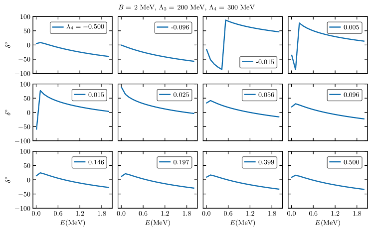
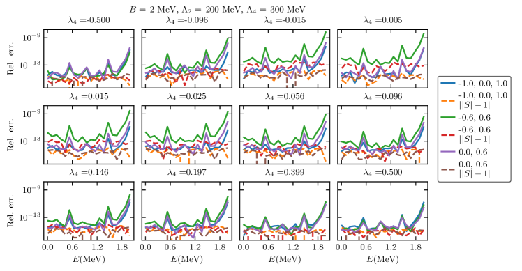
Figure 2: Particle-dimer s-wave scattering phase shifts vs. scattering energy $E$ for different $\lambda_{4}$ values (three-body interaction strength). The two-body interaction has fixed $\Lambda_{2}=200\,$MeV, and $\lambda$ is determined by the dimer binding energy $B=2\,$MeV. $\Lambda_{4}$ is fixed at 300 MeV.

Figure 3: The EC emulator errors for various $\lambda_{4}$ values (shown at the top of each panel), for which the exact phase shifts have been plotted in Fig. 3. Three different training sets have been used for constructing the EC emulators. Their $\lambda_{4}$ values are shown in the legends. The solid curves are the relative errors of the $S$ matrix, while the dashed curves plot $||S|-1|$, i.e., the unitarity violation.

Figure 3 shows the particle-dimer scattering phase shifts for the nucleon case, for 12 representative $\lambda_{4}$ values with $\Lambda_{2}=200$ and $\Lambda_{4}=300$ MeV. The phase shifts are sensitive to $\lambda_{4}$ when $|\lambda_{4}|\lessapprox 0.1$, but beyond that the dependence becomes much weaker. This can be understood from Eq. (21); we can make the estimate,

$$\langle g_{4}|G_{0}(E)|g_{4}\rangle =-\frac{4\pi^{3}}{3\sqrt{3}}\left(\frac{M}{\Lambda_{4}^{2}}\right)^{2}\int_{0}^{\infty}dE_{4}\frac{E_{4}^{2}\,e^{-\frac{ME_{4}}{\Lambda_{4}^{2}}}}{E_{4}-E^{+}}$$

$$\sim-\frac{4\pi^{3}}{3\sqrt{3}}\approx-20,$$ (45)

which is independent of $M$ and $\Lambda_{4}$. Thus when $|\lambda_{4}|\gg\frac{1}{20}$, $\tau_{4}$ becomes independent of $\lambda_{4}$. Therefore, we always choose $|\lambda_{4}|\leq 0.5$ when defining our parameter space.

Three sets of training points have been tried: (1) $\lambda_{4}=\{-1,0,1\}$, (2) $\lambda_{4}=\{-0.6,0.6\}$, and (3) $\lambda_{4}=\{0,0.6\}$. The errors of thus trained emulators at the 12 points from Fig. 3 are shown in Fig. 3, with solid and dashed lines for the relative errors of $S$ and the unitarity-violation error ($||S|-1|$), respectively. The errors are tiny: the $S$ errors are mostly on the order of $10^{-13}$ and increase to $10^{-10}$ near the breaking-up threshold. For the third training, the test points with $\lambda_{4}<0$ should be considered as extrapolations, while the other tests points as interpolations. The errors are similar for both interpolations and extrapolations. The unitarity-violation errors are generally smaller than the $S$ relative errors, which is also true in all the tests discussed in this work.

Besides the great accuracy, the other benefit of the emulator is its extreme efficiency. As mentioned in Sec. II, since $\lambda_{4}$ is a linear parameter in $V_{4}$, the $\delta U$ matrix can be computed once for a particular $\lambda_{4}$ value and then stored in the training period. At the emulating stage, the stored (low-dimensional) $\delta U$ can be rescaled quickly to get the correct $\delta U$ for the emulation point. The computational cost of the emulator is $10^{-3}$ seconds, which is for solving the $N_{b}$-dimensional linear equations in Eqs. (13) and (14). The memory costs during emulation are tiny. For example, the memory for storing $\delta U$ with $N_{b}=2$ and $3$ is negligible (cf. Table 1).

Such a scenario applies directly to the fitting of the low-energy constants in chiral three-nucleon interactions to measurements of $N$-$d$ scattering. Thus the EC emulators could play a key role in a full Bayesian treatment of these interactions. The generalization of the EC emulator to the energy region above the breakup-threshold, including for both elastic scattering and break-up reactions, will be desirable as well for this purpose and perhaps will help to resolve the long-standing $A_{y}$ puzzle Hebeler (2021).

IV.2 Vary $\lambda_{4}$ and $\Lambda_{4}$

Figure 4: The EC emulator errors for a few test points in the two-dimensional parameter space for the nucleon case. The solid and dashed curves in the same color are the $S$ matrix relative errors and the unitarity violation errors respectively with a fixed $N_{b}$ (see the legend). Here $B=2$ MeV and $\Lambda_{2}=200$ MeV. $\Lambda_{4}$ varies between 200 and 500 MeV, with $|\lambda_{4}|\leq 0.5$.

To further challenge the emulators, we now test them in a two-dimensional parameter space. The (nucleon case) parameter space is chosen with $|\lambda_{4}|\leq 0.5$ and $200\leq\Lambda_{4}\leq 500$ MeV and with $\Lambda_{2}=200$ MeV fixed.

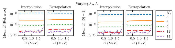
Figure 5: The mean of the EC emulator errors (the left two for $S$ and the right two for the unitarity violation) in the two-dimensional parameter space for the same five training sets as in Fig. 4 (see legend). In total, 200 points have been sampled and tested. $\Lambda_{2}$ is fixed at 200 MeV. The number of interpolation points grows with $N_{b}$. For $N_{b}=14$, the interpolation and extrapolations have a similar number of points.

In Fig. 4, the emulator errors at eight representative points in the parameter space are shown. On the top of each panel are the $\lambda_{4}$ and $\Lambda_{4}$ values of the test point. The training points are chosen using Latin hypercube sampling Tang (1993). The solid and dashed lines are the $S$ errors and the unitarity violation errors, respectively. In general, the latter are always smaller than the former. With six training points, the errors are of the order of $10^{-6}$. (Note that in solving the linear equations in Eqs. (13) and (14), a simple nugget $\sim 10^{-20}$ is added to the coefficient matrix to mitigate the ill-conditioning problem Furnstahl et al. (2020).)

To verify that these errors represent the global emulation accuracy, 200 test points are uniformly sampled in this two-dimensional parameter space. The mean values of the $S$ errors and their unitarity violations of the test samples are plotted in Fig. 5. The resulting mean values at different $N_{b}$ are consistent with what is seen in Fig. 4.

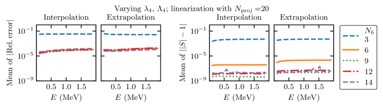
Figure 6: The mean of the errors of the EC emulators in the two-dimensional parameter space, which uses the Lagrange functions for the Legendre polynomials at $N_{\text{proj}}$ order to project the three-body interaction. $N_{\text{proj}}$ is fixed at 20. The training sets and the test point sample are the same as those in Fig. 5.

The $\Lambda_{4}$ dependence cannot be factorized from the three-body potential operator, so the EC emulators require re-computing the $\delta U$ matrix at all emulation points. The cost is minimized in the present work because of the use of separable potentials. In realistic calculations, the cost could be substantial and slows down the EC emulators significantly. To reduce this cost, our first approach is to decompose the varying potentials into a linear combination of basis potentials. Here, we work directly with the interaction form factor, $g_{4}(P,q)$, as a function of two variables in momentum space. (For non-separable potentials, the potentials need to be decomposed instead.) The form factor is decomposed into the products of the Lagrange functions of Legendre polynomials at order $N_{\text{proj}}$ Baye (2015):

$$g_{4}(P,q) =\sum_{m,n=0}^{N_{\text{proj}}-1}f_{nm}L_{n}(x_{p})L_{m}(x_{q}),$$ (46)

$$f_{nm} =g_{4}(P_{n},q_{m}).$$ (47)

In the numerical calculations, $P$ and $q$ are restricted to be between 0 and a large momentum cut-off $\Lambda_{\text{cut}}$. The $x_{p}$ and $x_{q}$ variables used in the Lagrange functions are simply $x_{p}\equiv 2P/\Lambda_{\text{cut}}-1$ and $x_{q}\equiv 2q/\Lambda_{\text{cut}}-1$. The coefficients $f_{m,n}$ are the values of $g(P,q)$ at the mesh points—defined as the zeros of the Legendre polynomial that generates the Lagrange functions Baye (2015). For the potential basis, $L_{n}(x)$ can be other functions, such as orthogonal polynomials, but inferring $f_{nm}$ could be more involved and thus increase the emulator time cost.

Figure 6 shows the mean of the errors of the EC emulator with the $g_{4}$ linearization for the same test-point sample as used in Fig. 5. The relative errors for $S$ have increased to $10^{-4}$—still useful for most data analysis—while the unitarity violation has smaller errors in general. The emulator cost is about $10^{-3}$ to $10^{-2}$ seconds per evaluation on a laptop computer.

Unsurprisingly, by increasing $N_{\text{proj}}$ large enough (up to $50$ here), the decomposition error reduces below the error of variational calculation; the new emulator errors become similar to the original EC errors in Figs. 5. However, the computational costs of training emulators grows with $N_{\text{proj}}^{2}$ (although such training calculations can be easily parallelized). The right balance between the training cost and the emulation accuracy has to be determined for each application of this emulator.

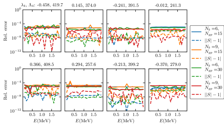
Figure 7: The GP-EC emulator errors for a few test points (the same as those in Fig. 4) in the two-dimensional parameter space. The emulators implement GP interpolation within the EC emulators. The solid and dashed curves in the same color are the $S$ errors and the unitarity violation errors, respectively, with a pair of fixed $N_{b}$ and $N_{gp}$ (see the legend).

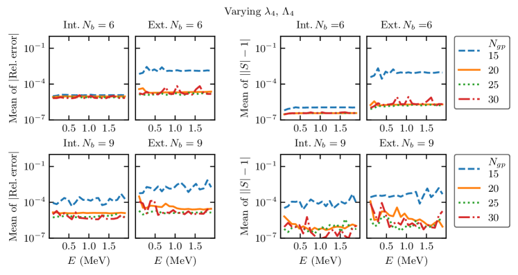
Figure 8: The mean of the GP-EC emulator errors. The emulators implement GP interpolation within the EC emulators. The top (bottom) panel has $N_{b}=6$ ($9$). Four different sizes of GP training sets from 15 to 30 are used in all the panels.

A second approach to deal with the non-factorizable parametric dependence is to use Gaussian processes (GPs) MacKay (1998) to interpolate $\delta U$ matrix elements in the parameter space. We call this a GP-EC emulator (it is also mentioned as the “nonlinear-1” case in Table 1). Even though the parameter space is two-dimensional, the GP only needs to be trained in the $\Lambda_{4}$ dimension, while the $\lambda_{4}$ dependence in $\delta U$ is linear and thus can be interpolated simply by rescaling. Note the $\lambda_{4}$ dependence of the $S$ matrix is still nonlinear. In short, when interpolating $\delta U$ instead of the final observables using the GP, the dimension of the interpolating space can be reduced by eliminating the dimension with linear dependence.

At the training stage, the GP is trained for each individual matrix element separately in the current work. The GPy package GPy (2012) is utilized; the default model optimization is applied to get the “best” GP interpolants. It is worth noting that principle component analysis can be used in the GP training Higdon et al. (2008) when the number of $\delta U$ matrix elements becomes large.

In Fig. 7, different combinations of the number of EC training points $N_{b}$ and the number of the GP training points $N_{gp}$ are explored; the emulator errors for the 8 different test points—the same as in Fig. 4— are shown there. With $N_{b}=9$ and $N_{gp}=30$, the errors are on the order of $10^{-5}$ (and the unitarity violation errors are even smaller). Fig. 8 shows the mean values of these errors with increasing $N_{gp}$, for the same test point sample as used in Fig. 5. The left two and right two panels show the $S$ errors and the unitarity violation errors, respectively, while the top and bottom panels have $N_{b}=6$ and $9$ separately. The interpolation and extrapolation errors are similar and below $10^{-5}$ when $N_{gp}\sim 20$; increasing $N_{gp}$ further does not further reduce the errors. This indicates that the GP-EC emulator errors are dominated by the GP interpolation errors. New ways to reduce GP errors will be explored in the future.

Meanwhile, the computational costs at the emulating stage include those for the trained GP to make predictions for $\delta U$ matrix elements and for solving the EC emulator linear equations. The total time cost is still only milliseconds. The memory costs for storing the trained GP emulators are a few MBs (c.f. Table 1), while those for solving Eqs. (13) and (14) are much smaller. The costs for training the emulators are detailed in Sec. IV.4.

The emulators studied in this section are suitable for fitting three-body interactions in three-cluster models that describe nuclear elastic scattering and reactions. The potential-linearization trick is not restricted to the Lagrange function basis. If the variation of the interaction range in the parameter space is small, other forms of basis may be available for reducing $N_{\text{proj}}$. The GP-EC emulator method can be applied as well. It will be interesting to compare them in realistic data fittings.

IV.3 Vary both $V_{4}$ and $V_{1,2,3}$: the “nonlinear-2” case

There exist situations where constraining two-body interactions between reactions subsystems requires input from three-body systems. For example, neutron-nucleus interactions are typically inferred from $d$-nucleus scatterings, because the direct experimental measurements of neutron-nucleus interactions are difficult. With this possibility in mind, we construct emulators for varying $\lambda_{4}$, $\Lambda_{4}$, and $\Lambda_{2}$ at the same time. The two-body binding energy $B$ is always fixed ($\lambda$ depends on $\Lambda_{2}$ as a result), as explained earlier.

Simply generalizing the EC emulators, however, faces a difficulty: the scattering wave functions of the training points and emulation points generally have different dimer bound-state wave functions. On the other hand, the functional in Eq. (35) requires the dimer bound-state wave function to be fixed while varying the trial wave function (see Eq. (38)).

To solve this problem, the dimer bound-state wave function within the training wave function in the asymptotic region is substituted by the dimer bound state of the emulation point. Meanwhile, in the interaction region the training wave functions are kept intact. The trial wave function built out of the linear combination of the new training wave functions (now labeled as $\tilde{\Psi}^{(i)}$) can be directly plugged into the functional in Eq. (35). Each modified training wave function is now

$$\tilde{\Psi}^{(i)} \equiv\sum_{\mu}\left(\psi_{(i),\mu}-\psi^{\mathrm{asym}}_{(i),\mu}+\tilde{\psi}^{\mathrm{asym}}_{(i),\mu}\right),$$ (48)

with the asymptotic FC $\psi^{\mathrm{asym}}_{(i),\mu}$ defined in Eq. (34) (in momentum space) and Eq. (70) (in coordinate space) and the modified asymptotic FC $\tilde{\psi}^{\mathrm{asym}}_{(i),\mu}$ defined in the same way. The difference between $\psi^{\mathrm{asym}}_{(i),\mu}$ and $\tilde{\psi}^{\mathrm{asym}}_{(i),\mu}$ is in their dimer bound-state wave functions: $\varphi_{(i),B}$ determined by the two-body potential of the training point and $\varphi_{B}$ determined by the emulation point.

Meanwhile, at small $R_{\mu}$ the full wave functions $\Psi_{(i)}$ and the two asymptotic wave functions $\sum_{i}\psi^{\mathrm{asym}}_{(i),\mu}$ and $\sum_{i}\tilde{\psi}^{\mathrm{asym}}_{(i),\mu}$ have the correct behavior, as shown in Eq. (37). Thus, the modified training wave functions $\tilde{\Psi}^{(i)}$ have the correct behavior as well.

In short, the $\tilde{\Psi}^{(i)}$ now satisfy the requirements for the trial wave functions in the variational calculations (c.f.  Sec. III.3), even though they are not eigenstates of the training Hamiltonian anymore. Based on these satisfied boundary conditions, we get an interesting and useful corollary, by repeating the derivations leading to Eq. (41):

$$\langle\tilde{\Psi}_{\bm{P}_{\mathrm{in}}}^{(i)}|E-H|\tilde{\Psi}_{\bm{P}_{\mathrm{in}}}^{(j)}\rangle-(i\leftrightarrow j)=3i\mathcal{N}^{2}\left(S^{(i)}-S^{(j)}\right).$$ (49)

This property guarantees that the EC emulator errors are exactly zero for the emulation point that is the same as one of the training points. Note that the corollary is also valid in the previous two emulator cases.

Equation (71) provides the working formula for computing $\delta U$. When the two-body interactions are not varied, the matrix element in Eq. (71) becomes a linear combination of the matrix elements of $V_{4}^{(j)}$ and $V_{4}$ at the emulation point. When varying $V_{1,2,3}$, a significant number of extra steps need to be taken (see the SM for more details). The numerical violation of Eq. (49) is used here to check the accuracy of the numerical overlap integrals in computing $\delta U$. Interestingly, all the overlap integrals are only nonzero at finite range. The range is determined by the ranges of the interactions as well as the size of the dimer bound state, which is consistent with the physical intuition for a particle scattering off a compound system.

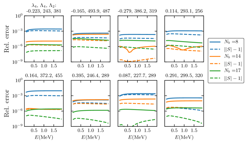
Figure 9: The EC emulator errors for a few test points in the three-dimensional parameter space with increasing $N_{b}$. The solid and dashed curves in the same color are the $S$ matrix’s relative errors and the unitarity violation errors respectively with a fixed $N_{b}$ (see legend).

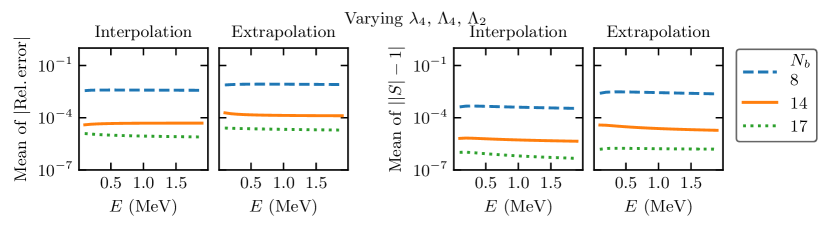
Figure 10: The mean of the EC emulator errors in the three-dimensional parameter space with the same training sets as in Fig. 9 (see legend).

Similar to Fig. 4, Fig. 9 shows the errors of the EC emulator for 8 different test points but now in the three-dimensional parameter space. The space is defined by $200\leq\{\Lambda_{2},\Lambda_{4}\}\leq 500$ MeV and $|\lambda_{4}|\leq 0.5$. With only $N_{b}=8$, the $S$ errors are no worse than one percent; the unitarity violation errors are even smaller. When $N_{b}=17$, the $S$ errors are reduced to at most $10^{-5}$.

In Fig. 10, 1000 test points in the three-dimensional parameter space are sampled uniformly. The test points enclosed by the training points are again considered as interpolations, while the others are extrapolations. The plot shows the mean of the errors for both samples, which are consistent with those seen for the 8 test points in Fig. 9. The interpolation and extrapolation errors are similar when $N_{b}$ becomes large enough.

It turns out that the emulator errors are dictated by our current numerical error in computing the overlap integrals in Eq. (71), which are more difficult than the calculations in the previous sections. By using Eq. (49), we found the integral errors and the emulator errors have similar magnitudes.

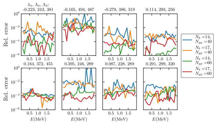
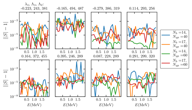
Figure 11: The GP-EC emulator relative errors for the same test points as in Fig. 9, in the three-dimensional parameter space. Four different combinations of $N_{b}$ and $N_{gp}$ are explored (see the legend).

Figure 12: The same as Fig. 12, but for the unitarity violation errors of the GP-EC emulators.

Even though these EC emulators have excellent accuracy, the calculation of $\delta U$ needs to be performed at each emulation point because of the extra modification applied to the training wave functions. This slows down the emulators dramatically. Therefore, the GP-EC emulator approach is employed here. For the GP-based emulation—again by using the GPy package GPy (2012)—of the $\delta U$, the effective dimension of the parameter space is reduced to either 1 or 2, by taking advantage of the presence of the linear parameter dependencies in $\delta U$.

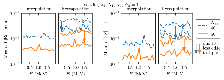
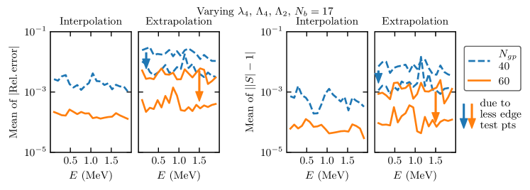
Figure 13: The mean of the GP-EC emulator errors vs $E$ in the three-dimensional parameter space, with $N_{b}=14$ and different $N_{gp}$. Two different calculations are performed: the first based on the same 1000 test point sample as used in Fig. 10 with $\Lambda_{2}$ and $\Lambda_{4}$ in $[200,500]$ MeV (318 interpolation and 682 extrapolation points) and the second with $\Lambda_{2}$ and $\Lambda_{4}$ in a smaller $[230,470]$ MeV range (312 interpolation and 325 extrapolation points). As can be seen, reducing the number of the edge test points reduces the errors in the extrapolation sample to a similar level as those in the interpolation sample.

Figure 14: The same as Fig. 14, but with $N_{b}=17$. For the full (smaller) sample, there are 322 (302) interpolation and 678 (335) extrapolation points. Similar to Fig. 14, reducing the number of the edge test points reduces the errors in the extrapolation sample to the same level as those in the interpolation sample.

Similar to Fig. 4, Figs. 12 and 12 show the errors of the GP-EC emulator with four different combinations of $N_{b}$ and $N_{gp}$ for the same 8 test points as shown in Fig 9. By comparing Figs. 12 and 9, we can see that the GP-EC emulator errors are dominated by those of the GP emulations. Therefore, the most significant accuracy improvement comes from increasing $N_{gp}$, not from increasing $N_{b}$ with fixed $N_{gp}$. Another important observation can be made: the errors for the test points near the edge of the parameter space (called “edge test points”), such as the one for panel (2), are significantly larger than those for the interior points. This is due to the large extrapolation errors of the GP emulation.

Figures 14 and 14 show the mean of the errors for $N_{b}=14$ and $N_{b}=17$, respectively. The interpolation and extrapolation points are defined in the same way as in Sec. IV.2. Increasing $N_{gp}$ from 40 to 60 reduces the errors from $10^{-3}$ ($10^{-2}$) to $10^{-4}$ ($10^{-3}$) for the interpolation (extrapolation) points. We further exclude the edge test points by restricting $\Lambda_{2}$ and $\Lambda_{4}$ to a narrower range, $[230,470]$ MeV. The mean of the errors for the interpolations are not changed, but for the extrapolations the mean gets reduced to a similar level as that of the interpolation points, which is consistent with the observation we made for Fig. 12. It also suggests that to improve the emulation accuracy, the parameter space for training should be chosen larger than for emulation.

By employing the GP emulation of $\delta U$, the full time cost of the GP-EC emulator for this case is on the order of milliseconds. In comparison, the original EC emulator takes $10^{3}$ seconds for each evaluation. The memory costs are larger—from 10s up to 100 MB—than the GP-EC costs in Sec. IV.2, caused by the larger $N_{b}$ and $N_{\mathrm{gp}}$ here.

IV.4 Training costs

The computing costs for training the emulators are another important factor to be considered. Since they are highly dependent on the complexity of the three-body problem, we concentrate on their scaling with the training parameters and potential parallelizations of the training computations.

The cost budget—at a single scattering energy—for the “nonlinear-2” emulator has three main parts: the first for directly solving the scattering problem at $N_{b}$ EC training points, the second for computing $\delta U$ at $N_{gp}$ GP training points, and the last for training the GPs using the GPy package. The first costs are proportional to $N_{b}$—on the order of 10 for the emulation in the three-dimensional space! These $N_{b}$ calculations are mutually independent and can be readily parallelized.

The second costs scale as $N_{b}^{2}\,N_{gp}$. They could also be significant but can be easily parallelized as well into $N_{b}^{2}\,N_{gp}$ independent calculations. The procedure of correcting the training wave functions’ asymptotic behavior does not increase the second costs in any significant way. The two-body bound state problem can be either fully solved quickly—as implemented in this work—or by using a bound-state EC emulator König et al. (2020); Ekström and Hagen (2019). The GP training costs scale as $N_{b}^{2}\,N_{gp}^{3}$, however the calculations can be parallelized into $N_{b}^{2}$ independent ones.

The “nonlinear-1” emulator has the same training budget structure, but the training calculations are simpler. The “linear” emulator costs the least without using GP.

V Summary and outlook

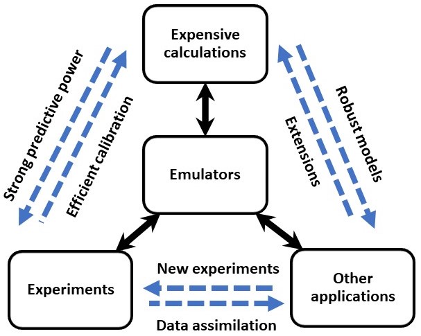
Figure 15: The emulator’s role in the workflow for nuclear physics and other research areas. The dashed arrows indicate desirable connections enabled by the emulators.

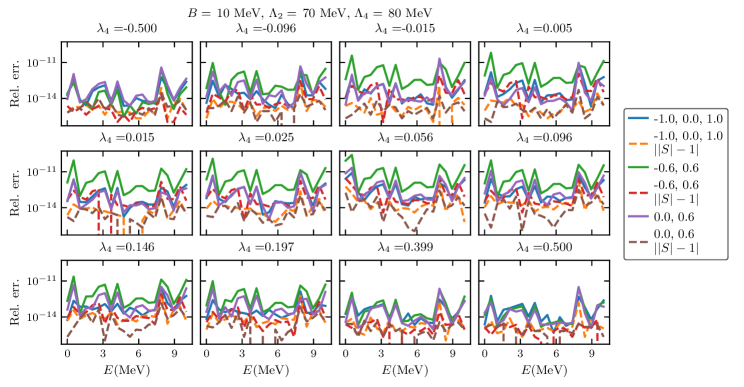
Figure S2: The EC emulator errors for various $\lambda_{4}$ values (shown at the top of each panel), for which the exact phase shifts have been plotted in Fig. S1. Three different training sets have been used for constructing the EC emulators. Their $\lambda_{4}$ values are shown in the legends. The solid curves are the relative errors of the $S$ matrix, while the dashed curves plot the unitarity violation.

In this work, we have developed fast emulators for quantum three-body scattering by combining the variational method and the EC concept. Different variants of the emulators are studied in anticipation of different application scenarios. Their accuracy and computing costs are summarized in Table 1, and discussed in detail in Sec. IV: the emulator errors in Figs. 3, 8, 14, and 14 (and Figs. S2, S6, S7, S12, and S13 for the nuclear case), the emulator computing costs in the discussions of these figures, and their training costs in Sec. IV.4. (The codes to generate the results presented in this paper will be made public BUQEYE collaboration .)

In Sec. IV.2, two different solutions are explored to expedite the EC emulators that get slowed down due to the nonfactorizable parametric dependence of the varying interactions within the Hamiltonian. One uses Lagrange functions to linearly decompose the interaction operators (see Eq. (46)), while the other—called a GP-EC emulator—employs GP emulation of the $\delta U$ matrix. The GP-EC emulators are again applied in Sec. IV.3 to achieve fast emulation. The section also demonstrates a working procedure to correct the asymptotic behavior of the trial wave functions when building the emulators.

Now, we comment on a few important and interesting generalizations and their potential impact in nuclear physics and beyond.

To emulate $N$-$d$ and $d$-nucleus scattering, as well as any processes that can be modeled as three-cluster systems, the current emulators need to be extended to include spin and isospin degrees of freedom, fermion statistics, and higher partial waves (or even full scattering amplitude without partial wave decomposition). It will also be useful to generalize the emulators for the energy region above the dimer break-up threshold and to include scattering, nuclear excitation, and dimer breakup channels. Constructing EC emulators for four- and higher-body scatterings is another interesting topic.

Our current estimates of the emulation accuracy and costs, as outlined in Table 1, should be good guides for the future emulations of the realistic calculations mentioned above. The essential question is how the numbers of trainings—determining both accuracy and costs—extrapolate from the present work to realistic calculations. In the EC emulation of the many-body nuclear structure calculation in Ref. Ekström and Hagen (2019), $N_{b}\sim 60$ trainings were employed in a 16-dimensional parameter space of the chiral nucleon interaction theory to achieve percent-level emulation accuracy. For such $N_{b}$, which are only a few times of the largest $N_{b}=17$ used here (in the “nonlinear-2” case), we expect the estimates in Table 1 to hold within an order of magnitude.

Such emulators have the potential to create a new workflow in nuclear physics research and in other fields, as implied by the diagram in Fig. 15. Although our focus is the three-body quantum scattering problem, the workflow diagram and its discussion could apply in other situations, such as higher-body scattering and many-body bound-state studies.

Calculations starting from more microscopic physics generally promise physics modeling with great predictive power, less model dependence, and more complete uncertainty quantification. These advantages are desirable, but their expensive computational costs have frequently kept their interactions with other sectors (the other two blocks in Fig. 15) from growing stronger. This means a loss of novel research opportunities.

Developing efficient and accurate emulators will fundamentally change this situation. As the proxy of the expensive calculations, they can be coupled to data analysis and other applications, thanks to their low computational costs. Novel studies could emerge with the fostering of new interactions between different research areas. For example, three-body emulators will enable direct applications of Faddeev scattering equations in experimental data analysis, experimental design, and the efficient calibration of theory.

The “other applications” in Fig. 15 include collaborations with other theoretical approaches, either more or less microscopic than the “expensive calculations”. For the three-nucleon emulators, they could be Lattice-QCD calculations or a two-body study that treats the deuteron as a single particle degrees of freedom.

In collaborations, “expensive calculations” provide robust models for other approaches to compare with, and in return extend the range of their own applications. An important part of working with different approaches is in fact data analysis, i.e., constraining the macroscopic theories and models with the information from more microscopic ones. The three-nucleon emulators can be applied to extract three-nucleon interactions from Lattice-QCD calculations, an approach that is different from current generalizations of the Lüscher method Jackura et al. (2019). Similarly, matching three-cluster theories and many-body structure calculations can create a new method of ab initio nuclear scattering calculation, a desirable generalization of the recent two-cluster study Zhang et al. (2020b).

Through the emulators of the “expensive calculations”, the “experiments” and “other applications” are efficiently coupled as well. This allows the assimilation of experimental data into theoretical studies, which in return could create new experimental proposals. The three-nucleon emulators could provide a robust connection between $N$-$d$ scattering measurements and the three-nucleon energy levels computed in Lattice-QCD.

By merging variational methods with the EC principle, a new way to construct emulators is opened up. This strategy is fundamentally different from those based on GPs or neural networks, as used in machine learning. The EC emulators take into account the physics involved through variational methods, while the others learn the physics based on statistical methods. The new strategy may not have as broad applications, but whenever applicable, the EC emulators could have much better accuracy for both interpolations and extrapolations.

Note: recently another type of three-nucleon scattering emulator was proposed in Ref. Witała et al. (2021). The emulator is based on a lowest-order perturbative treatment of the varying potential operators, in particular the contact three-nucleon interactions. The application scenario is the same as the “linear” case in Table 1. The emulation accuracy is on the percent level and the time costs are seconds on a personal computer.

Appendix A Conventions for states

Single-particles states in coordinate and momentum space satisfy

$$\langle\bm{p}^{\prime}|\bm{p}\rangle =\delta(\bm{p}-\bm{p}^{\prime}),$$ (50)

$$\langle\bm{r}^{\prime}|\bm{r}\rangle =\delta(\bm{r}-\bm{r}^{\prime}),$$ (51)

$$\langle\bm{r}|\bm{p}\rangle =\frac{e^{i\bm{p}\bm{r}}}{\sqrt{\left(2\pi\right)^{3}}}.$$ (52)

The partial wave bases are defined through

$$\langle\bm{p}^{\prime}|p,\ell,m\rangle =\frac{\delta(p^{\prime}-p)}{p^{2}}Y_{\ell m}(\hat{p}^{\prime}),$$ (53)

$$\langle\bm{r}^{\prime}|r,\ell,m\rangle =\frac{\delta(r^{\prime}-r)}{r^{2}}Y_{\ell m}(\hat{r}^{\prime}).$$ (54)

It can be verified that

$$\langle p^{\prime},\ell^{\prime},m^{\prime}|p,\ell,m\rangle =\frac{\delta(p^{\prime}-p)}{p^{2}}\delta_{\ell\ell^{\prime}}\delta_{mm^{\prime}},$$ (55)

$$\langle\bm{r}|p,\ell,m\rangle =\sqrt{\frac{2}{\pi}}i^{\ell}Y_{\ell m}(\hat{r})j_{\ell}(pr).$$ (56)

Let us turn to the states in the three-body system. The CM degree of freedom, which is always factorized from the full state, is kept implicit in the states. The states are now labeled by two kinematic variables—either coordinate or momentum—for the relative motions, as shown in Fig. 1 and discussed in the beginning of Sec. III.1. There are three equivalent sets of kinematic variables describing the same system. The variables are linearly related. For the case with the same mass for all particles, they are Glöckle (1983):

$$\bm{R}_{2} =-\frac{1}{2}\bm{R}_{1}+\frac{3}{4}\bm{r}_{1},\quad\bm{r}_{2}=-\bm{R}_{1}-\frac{1}{2}\bm{r}_{1},$$

$$\bm{R}_{3} =-\frac{1}{2}\bm{R}_{1}-\frac{3}{4}\bm{r}_{1},\quad\bm{r}_{3}=\bm{R}_{1}-\frac{1}{2}\bm{r}_{1}.$$ (57)

Importantly, for $R_{1}$ (or $r_{1}$) approaching $+\infty$, the other variables approach $+\infty$ as well.

The index outside of a state, such as $i$ in $|{}\rangle_{i}$, identifies the particular choice of coordinate system. Thus, $|\bm{R}_{1},\bm{r}_{1}\rangle_{1}$ means using the coordinate system with particle $1$ as spectator, with $\bm{r}_{1}$ and $\bm{R}_{1}$ for the relative coordinates between particle 2 and 3 and between 1 and the CM of 2 and 3, respectively. In contrast, $|\bm{R}_{2},\bm{r}_{2}\rangle_{1}$ has $\bm{r}_{2}$ and $\bm{R}_{2}$ for the relative coordinates between particle 2 and 3 and between 1 and the CM of 2 and 3 (not between particle 1 and 3 and between 2 and the CM of 1 and 3). Of course, $|\bm{R}_{\mu},\bm{r}_{\mu}\rangle_{\mu}$ with $\mu=1,2,3$ are the same state. The momentum space states are defined in the same way. In order to simplify the notation, the $|\bm{R}_{1},\bm{r}_{1}\rangle_{1}$ basis state will have index $1$ omitted, and the other states, such as $|\bm{P}_{\gamma},g_{\gamma}\rangle$, rely on the index $\gamma$ to label the coordinate system, whenever doing so doesn’t cause confusion.

Appendix B Three-body scattering wave functions

Detailed discussions of the Faddeev equations can be found in Ref. Glöckle (1983). Here we focus on computing scattering wave functions based on half-off-shell transition amplitudes, $X$, and the asymptotic behavior of the wave functions in coordinate space.

We start with the $V_{4}=0$ case. The Faddeev components are defined as

$$|\psi_{\alpha,\mu}\rangle \equiv G_{0}V_{\mu}|\Psi_{\alpha}^{(+)}\rangle,$$ (58)

$$\sum_{\mu}|\psi_{\alpha,\mu}\rangle =G_{0}\left(\sum_{\mu}V_{\mu}\right)|\Psi_{\alpha}^{(+)}\rangle=|\Psi_{\alpha}^{(+)}\rangle,$$ (59)

with $\mu=1,2,3$. To get the expressions for $\psi_{\alpha,\mu}$, we can now multiply Eq. (17) by $G_{0}$ from the left. For $\alpha=1$, we have

$$|\psi_{1,1}\rangle =\frac{1}{2}G_{0}\left(U_{21}+U_{31}-U_{11}\right)|\phi_{1}\rangle\$$

$$=G_{0}|\bm{P}_{1},\hat{g}_{1}\rangle+G_{0}t_{1}G_{0}U_{11}G_{0}|\bm{P}_{1},\hat{g}_{1}\rangle,$$ (60)

$$|\psi_{1,2}\rangle =\frac{1}{2}G_{0}\left(U_{11}+U_{31}-U_{21}\right)|\phi_{1}\rangle\$$

$$=G_{0}t_{2}G_{0}U_{21}G_{0}|\bm{P}_{1},\hat{g}_{1}\rangle,$$ (61)

$$|\psi_{1,3}\rangle =\frac{1}{2}G_{0}\left(U_{11}+U_{21}-U_{31}\right)|\phi_{1}\rangle\$$

$$=G_{0}t_{3}G_{0}U_{31}G_{0}|\bm{P}_{1},\hat{g}_{1}\rangle.$$ (62)

These expressions can be generalized to Watson and Nuttall (1967)

$$|\psi_{\alpha,\mu}\rangle =\delta_{\alpha\mu}G_{0}|\bm{P}_{\alpha},\hat{g}_{\alpha}\rangle+G_{0}t_{\mu}G_{0}U_{\mu\alpha}G_{0}|\bm{P}_{\alpha},\hat{g}_{\alpha}\rangle.$$ (63)

When $V_{4}\neq 0$, the aforementioned FCs cannot be summed to get the full wave function. A fourth FC $|\psi_{1,4}\rangle\equiv G_{0}V_{4}|\Psi_{1}^{(+)}\rangle$ can be temporarily introduced. By repeating the derivations that leads to Eq. (60), (61) and (62), we get the same expressions for $\psi_{1,\mu}$ for $\mu=1,2,3$ and in addition,

$$|\psi_{1,4}\rangle =\frac{1}{3}G_{0}\left(U_{11}+U_{21}+U_{31}-2U_{41}\right)|\phi_{1}\rangle$$

$$=G_{0}t_{4}G_{0}U_{41}G_{0}|\bm{P}_{1},\hat{g}_{1}\rangle\$$

$$=\bigg{(}G_{0}t_{4}+G_{0}t_{4}\sum_{\beta}G_{0}t_{\beta}G_{0}U_{\beta 1}\bigg{)}G_{0}|\bm{P}_{1},\hat{g}_{1}\rangle.$$ (64)

In the last step, the following identity is invoked Glöckle (1983):

$$U_{4\alpha} =G_{0}^{-1}+\sum_{\gamma}t_{\gamma}G_{0}U_{\gamma\alpha}.$$ (65)

This suggests a new way to represent the full wave function, by adding all the pieces of $|\psi_{1,4}\rangle$ to the other three FCs. We finally have Eq. (26) for general channel $\alpha$.

For identical bosons, the symmetrized FC is (see Sec. III.2)

$$|\psi_{\mu}\rangle=\sum_{\alpha}|\psi_{\alpha,\mu}\rangle=(1+G_{0}t_{4})\,G_{0}|\bm{P}_{\mu},\hat{g}_{\mu}\rangle+\sum_{\alpha}(1+G_{0}t_{4})\,G_{0}t_{\mu}G_{0}U_{\mu\alpha}G_{0}|\bm{P}_{\alpha},\hat{g}_{\alpha}\rangle$$ (66)

In momentum space with e.g., $\mu=1$,

$$\langle\bm{P}_{1},\bm{q}_{1}|\psi_{\bm{P}_{\mathrm{in}},1}\rangle=\, \tilde{Z}_{d}(\bm{P}_{1},\bm{q}_{1})\delta(\bm{P}_{1}-\bm{P}_{\mathrm{in}})+\tilde{Z}_{14}(\bm{P}_{1},\bm{q}_{1})\,\tau_{4}(E)\,Z_{41}(\bm{P}_{\mathrm{in}})+\tilde{Z}_{d}(\bm{P}_{1},\bm{q}_{1})\,\hat{\tau}(E-\frac{P_{1}^{2}}{2\mu^{1}})\,X(\bm{P}_{1},\bm{P}_{\mathrm{in}})$$

$$+\tilde{Z}_{14}(\bm{P}_{1},\bm{q}_{1})\,\tau_{4}(E)\,\int d\bm{P}\,Z_{41}(\bm{P})\,\hat{\tau}(E-\frac{P^{2}}{2\mu^{1}})\,X(\bm{P},\bm{P}_{\mathrm{in}}),$$ (67)

with

$$\tilde{Z}_{d}(\bm{P}_{1},\bm{q}_{1})\equiv\, \frac{\hat{g}(\bm{q}_{1})}{E+i\epsilon-\frac{P_{1}^{2}}{2\mu^{1}}-\frac{q_{1}^{2}}{2\mu_{1}}},$$ (68)

$$\tilde{Z}_{14}(\bm{P}_{1},\bm{q}_{1}) \equiv\langle\bm{P}_{1},\bm{q}_{1}|G_{0}(E)|g_{4}\rangle.$$ (69)

Other quantities, including $Z_{41}$ and $\tau_{4}$, are defined in Sec. III.1.

The asymptotic behavior of the FCs at large particle-dimer separation, as shown in Eq. (32), is determined by their singularities in momentum space in Eq. (67), including the $\delta(\bm{P}_{1}-\bm{P}_{\mathrm{in}})$ term and the pole of $\hat{\tau}(E-P_{1}^{2}/2\mu^{1})$ in the third term when $P_{1}=P_{\mathrm{in}}$. The other terms proportional to $\tau_{4}$ decrease exponentially with $R_{1}$ and thus do not contribute to the asymptotic behavior, below the break-up threshold.

We can isolate these singularities by subtracting the FC with the asymptotic piece defined in Eq. (34). Within $\psi^{\mathrm{asym}}$, the large $P_{1}$ dependence of the $P_{1}=P_{\mathrm{in}}$ pole term is further regularized using the $\tilde{\Lambda}$ parameter. In coordinate space, the subtraction projected to s-waves is

$$\langle{R}_{1},{r}_{1}|\psi^{\mathrm{asym}}_{\bm{P}_{\mathrm{in}},1}\rangle =\frac{\mathcal{N}}{\sqrt{v}}\frac{u_{B}({r}_{1})}{r_{1}R_{1}}\bigl{(}-e^{-iP_{\mathrm{in}}R_{1}}+e^{2i\delta_{0}}e^{iP_{\mathrm{in}}R_{1}}$$

$$\quad\hbox{}-2i\sin\delta_{0}e^{i\delta_{0}}e^{-\tilde{\Lambda}R_{1}}\bigr{)}.$$ (70)

As can be seen, $\tilde{\psi}^{\mathrm{asym}}$ approaches to the FC’s asympototic behavior at large $R_{1}$, but meanwhile becomes finite when $R_{1}\to 0$, a boundary condition for a physical solution, thanks to the $\tilde{\Lambda}$-dependent regularization.

Appendix C Emulators

The following formula is used to compute $\delta U$ in constructing the EC emulators with varying $V_{1,2,3}$ and $V_{4}$:

$$\langle\tilde{\Psi}^{(i)}|E -H|\tilde{\Psi}^{(j)}\rangle=\langle\Psi^{\mathrm{sub}}_{(i)}|V^{(j)}-V|\Psi^{\mathrm{sub}}_{(j)}\rangle$$

$$\hbox{}+3\,\langle\Psi^{\mathrm{sub}}_{(i)}|V^{(j)}_{2}+V^{(j)}_{3}+V^{(j)}_{4}|\psi^{\mathrm{asym}}_{(j),1}\rangle$$

$$\hbox{}-3\,\langle\Psi^{\mathrm{sub}}_{(i)}|V_{2}+V_{3}+V_{4}|\tilde{\psi}^{\mathrm{asym}}_{(j),1}\rangle$$

$$\hbox{}-3\,\frac{P_{\mathrm{in}}^{2}+\tilde{\Lambda}^{2}}{2\mu^{1}}\langle\Psi^{\mathrm{sub}}_{(i)}|\Delta\psi^{\mathrm{asym}}_{(j),1}-\Delta\tilde{\psi}^{\mathrm{asym}}_{(j),1}\rangle$$

$$\hbox{}+\langle\tilde{\Psi}^{\mathrm{asym}}_{(i)}|V^{(j)}-V|\Psi^{\mathrm{sub}}_{(j)}\rangle$$

$$\hbox{}+3\,\langle\tilde{\Psi}^{\mathrm{asym}}_{(i)}|V^{(j)}_{2}+V^{(j)}_{3}+V^{(j)}_{4}|\psi^{\mathrm{asym}}_{(j),1}\rangle$$

$$\hbox{}-3\,\langle\tilde{\Psi}^{\mathrm{asym}}_{(i)}|V_{2}+V_{3}+V_{4}|\tilde{\psi}^{\mathrm{asym}}_{(j),1}\rangle$$

$$\hbox{}-3\,\frac{P_{\mathrm{in}}^{2}+\tilde{\Lambda}^{2}}{2\mu^{1}}\langle\tilde{\Psi}^{\mathrm{asym}}_{(i)}|\Delta\psi^{\mathrm{asym}}_{(j),1}-\Delta\tilde{\psi}^{\mathrm{asym}}_{(j),1}\rangle.$$ (71)

$\tilde{\Psi^{(i)}}$ is defined in Eq. (48). $V$ and $V^{(j)}$ are the full potential including both two and three-body interactions for the emulation point and the $j$th training point (labelled by $(j)$ in sub or superscripts) respectively. And $\Delta\psi^{\mathrm{asym}}_{(j),1}$ is the difference between the regularized asymptotic FC in Eq. (34) and the non-regularized one (i.e., the regularized one but with $\tilde{\Lambda}\to+\infty$):

$$\langle P_{1},q_{1}|\Delta\psi^{\mathrm{asym}}_{(j),1}\rangle \equiv\varphi_{B,(j)}(q_{1})\frac{8\pi\mu^{1}}{P_{1}^{2}+\tilde{\Lambda}^{2}}X_{(j)}(P_{\mathrm{in}},P_{\mathrm{in}}),$$ (72)

$$\langle P_{1},q_{1}|\Delta\tilde{\psi}^{\mathrm{asym}}_{(j),1}\rangle \equiv\varphi_{B}(q_{1})\frac{8\pi\mu^{1}}{P_{1}^{2}+\tilde{\Lambda}^{2}}X_{(j)}(P_{\mathrm{in}},P_{\mathrm{in}}),$$ (73)

$$\text{with}\ \varphi_{B,(j)}(q_{1}) \equiv\frac{\hat{g}_{(j)}({q})}{-B-\frac{q^{2}}{2\mu_{1}}},\ \varphi_{B}(q_{1})\equiv\frac{\hat{g}({q})}{-B-\frac{q^{2}}{2\mu_{1}}}.$$ (74)

In coordinate space, they become

$$\langle R_{1},r_{1}|\Delta\psi^{\mathrm{asym}}_{(j),1}\rangle =-\varphi_{B,(j)}(r_{1})e^{i\delta_{(i)}}\sin{\delta_{(i)}}\sqrt{\frac{2}{\pi}}\frac{e^{-\tilde{\Lambda}R_{1}}}{P_{\mathrm{in}}R_{1}},$$ (75)

$$\langle R_{1},r_{1}|\Delta\tilde{\psi}^{\mathrm{asym}}_{(j),1}\rangle =-\varphi_{B}(r_{1})e^{i\delta_{(i)}}\sin{\delta_{(i)}}\sqrt{\frac{2}{\pi}}\frac{e^{-\tilde{\Lambda}R_{1}}}{P_{\mathrm{in}}R_{1}}.$$ (76)

Note $\varphi_{B}(q_{1})$ and $\varphi_{B}(r_{1})$, for example, are the dimer bound-state wave function in momentum and coordinate space.

To derive Eq. (71), we make use of Eq. (48) and

$$(E-H)|\tilde{\Psi}^{(j)}\rangle =(E-H)|\Psi^{(j)}\rangle-(E-H)|\Psi^{\mathrm{asym}}_{(j)}\rangle$$

$$\quad\hbox{}+(E-H)|\tilde{\Psi}^{\mathrm{asym}}_{(j)}\rangle$$

$$=(V^{(j)}-V)\left(|\Psi^{\mathrm{sub}}_{(j)}\rangle+|\Psi^{\mathrm{asym}}_{(j)}\rangle\right)$$

$$\quad\hbox{}-(E-H)\left(|\Psi^{\mathrm{asym}}_{(j)}\rangle-|\tilde{\Psi}^{\mathrm{asym}}_{(j)}\rangle\right).$$ (77)

Because

$$(E-H_{0}-V_{1}^{(j)})|\psi^{\mathrm{asym}}_{(j),1}\rangle =\frac{P_{\mathrm{in}}^{2}+\tilde{\Lambda}^{2}}{2\mu^{1}}|\Delta\psi^{\mathrm{asym}}_{(j),1}\rangle,$$ (78)

$$(E-H_{0}-V_{1})|\tilde{\psi}^{\mathrm{asym}}_{(j),1}\rangle =\frac{P_{\mathrm{in}}^{2}+\tilde{\Lambda}^{2}}{2\mu^{1}}|\Delta\tilde{\psi}^{\mathrm{asym}}_{(j),1}\rangle,$$ (79)

we have

$$(E-H_{0})|\Psi^{\mathrm{asym}}_{(j)}\rangle =(E-H_{0})\sum_{\mu}|\psi^{\mathrm{asym}}_{(j)}\rangle$$

$$=\sum_{\mu}V_{\mu}^{(j)}|\psi^{\mathrm{asym}}_{(j),\mu}\rangle$$

$$\quad\hbox{}+\frac{P_{\mathrm{in}}^{2}+\tilde{\Lambda}^{2}}{2\mu^{1}}\sum_{\mu}\Delta\psi^{\mathrm{asym}}_{(j),\mu},$$ (80)

$$(E-H_{0})|\tilde{\Psi}^{\mathrm{asym}}_{(j)}\rangle =(E-H_{0})\sum_{\mu}|\tilde{\psi}^{\mathrm{asym}}_{(j)}\rangle$$

$$=\sum_{\mu}V_{\mu}|\tilde{\psi}^{\mathrm{asym}}_{(j),\mu}\rangle$$

$$\quad\hbox{}+\frac{P_{\mathrm{in}}^{2}+\tilde{\Lambda}^{2}}{2\mu^{1}}\sum_{\mu}\Delta\tilde{\psi}^{\mathrm{asym}}_{(j),\mu}.$$ (81)

Plugging the above formula into Eq. (77) gives Eq. (71).

Appendix A Additional details for the exact solutions of the three-body scattering problem

In the two body sector, the interaction form factor in coordinate space is

$$g(\bm{r})=g({r})=C\,\Lambda_{2}^{2}\exp\left[-\frac{\Lambda_{2}^{2}r^{2}}{2}\right].$$ (S1)

The $C$ in Eq. (S1) and (42) defining the Gaussian form factor is chosen such that at low-energy, the scattering length and effective range terms in the low energy effective range expansion (i.e., $p\cot\delta=-1/a_{0}+1/2\,r_{0}\,p^{2}+...$) become

$$-\frac{1}{a_{0}} =-\frac{\Lambda_{2}}{\sqrt{\pi}}\left(1+\lambda^{-1}\right),$$ (S2)

$$r_{0} =-\frac{2}{\Lambda_{2}}\left(\frac{1}{a_{0}\Lambda_{2}}-\frac{2}{\sqrt{\pi}}\right).$$ (S3)

The two-body scattering $T$-matrix at general energy $e_{2}$,

$$\tau^{-1}(e_{2}) =\lambda^{-1}-\langle g|G_{0}^{(2b)}(e_{2})|g\rangle$$ (S4)

$$\langle g|G_{0}^{(2b)}(e_{2})|g\rangle =(4\pi)\left(\frac{C}{\Lambda_{2}}\right)^{2}(-\Lambda_{2}\mu_{1})$$

$$\times\left.\bigl{[}\sqrt{\pi}-\pi\sqrt{D}\,e^{D}\,\operatorname{Erfc}\bigl{(}\sqrt{D}\bigr{)}\bigr{]}\right|_{D=-\frac{2\mu_{1}e_{2}^{+}}{\Lambda_{2}^{2}}}$$ (S5)

Note $G_{0}^{(2b)}$ is the two-body free Green’s function here.

$$e_{2}^{+} \equiv e_{2}+i0^{+},$$ (S6)

$$\operatorname{Erfc}\left(\sqrt{D}\right) =1-\operatorname{Erf}\left(-i\frac{k}{\Lambda_{2}}\right)=1+i\operatorname{Erfi}\left(\frac{k}{\Lambda_{2}}\right).$$ (S7)

The definitions of the error functions can be found in Ref. DLMF . Based on the expressions for the $T$-matrix, we can recover the relationships between effective range parameters and $\Lambda_{2},\lambda$ as just discussed above.

To get the dimer bound state properly normalized, the $\xi$ parameter is determined through ($B$ as the dimer’s binding energy)

$$\frac{1}{\xi^{2}} =\langle g|\left[G_{0}^{(2b)}(-B)\right]^{2}|g\rangle$$

$$=(4\pi)\left(\frac{C}{\Lambda_{2}}\right)^{2}\left(\frac{\mu_{1}}{\Lambda_{2}}\right)\left(2\mu_{1}\right)\Bigl{[}-\sqrt{\pi}$$

$$\hbox{}+\frac{\pi}{2\sqrt{D_{B}}}(1+2D_{B})\,e^{D_{B}}\,\operatorname{Erfc}(\sqrt{D_{B}})\Bigr{]}\Bigr{|}_{D_{B}=\frac{2\mu_{1}B}{\Lambda_{2}^{2}}}$$ (S8)

For the three-body potential, its form factor in coordinate space is

$$\langle\bm{R}_{1},\bm{r}_{1}|g_{4}\rangle =\int d\bm{P}_{1}d\bm{q}_{1}\frac{e^{i\left(\bm{P}_{1}\bm{R}_{1}+\bm{q}_{1}\bm{r}_{1}\right)}}{(2\pi)^{3}}\frac{1}{\sqrt{M\Lambda_{4}^{4}}}\exp\left[-\frac{ME_{4}}{2\Lambda_{4}^{2}}\right]=\frac{\Lambda_{4}^{4}}{\sqrt{M}}\frac{2\sin(2\phi)}{3R_{1}r_{1}}L^{2}\exp\left(-\frac{\Lambda_{4}^{2}L^{2}}{2}\right)\ \text{with}$$

$$K^{2} =ME_{4}=q_{1}^{2}+\frac{3}{4}P_{1}^{2},\quad L^{2}=\frac{4}{3}R_{1}^{2}+r_{1}^{2}\quad\text{and}\quad\sin\phi\equiv\frac{r_{1}}{L}$$ (S9)

When solving Eq. (28), we use the following analytical results.

$$Z_{21}(\bm{P}_{2},\bm{P}_{1}) =\frac{M\xi^{2}}{M(E+i\epsilon)-P_{1}^{2}-P_{2}^{2}-{P}_{1}{P}_{2}x}\left(\frac{C}{\Lambda_{2}}\right)^{2}\exp\left[-\frac{1}{\Lambda_{2}^{2}}\left(\frac{5}{8}P_{1}^{2}+\frac{5}{8}P_{2}^{2}+P_{1}P_{2}x\right)\right]$$ (S10)

$$Z_{21}({P}_{2},{P}_{1}) =\frac{1}{2}\int_{-1}^{1}dxZ_{21}(\bm{P}_{2},\bm{P}_{1})$$

$$=(-)\frac{\xi^{2}}{2}\frac{M}{P_{1}P_{2}}\left(\frac{C}{\Lambda_{2}}\right)^{2}\exp\left[-\frac{5}{8\Lambda_{2}^{2}}\left(P_{1}^{2}+P_{2}^{2}\right)\right]\left\{e^{\tilde{D}}\left[\Gamma\left(0,\tilde{D}-\tilde{d}\right)-\Gamma\left(0,\tilde{D}+\tilde{d}\right)\right]\right\}$$

with $$\tilde{D}=\frac{P_{1}^{2}+P_{2}^{2}-ME^{+}}{\Lambda_{2}^{2}},\quad\tilde{d}=\frac{P_{1}P_{2}}{\Lambda_{2}^{2}},\quad\text{and}\quad x\equiv\frac{\bm{P}_{1}\cdot\bm{P}_{2}}{P_{1}P_{2}}$$ (S11)

The definition of the incomplete Gamma function, $\Gamma(0,x)$ can be found in (DLMF, , Eq. 8.2.2).

In addition,

$$Z_{14}(\bm{P}) ={}_{1}\langle\hat{g},\bm{P}|G_{0}(E)|g_{4}\rangle=-4\pi M\xi\,\frac{C}{\Lambda_{2}}\frac{1}{\sqrt{M}\Lambda_{4}^{2}}\exp\left(-\frac{3P^{2}}{8\Lambda_{4}^{2}}\right)\,\frac{1}{2\sqrt{t}}\left[\sqrt{\pi}-\pi e^{D\,t}\sqrt{D\,t}\operatorname{Erfc}\left(\sqrt{D\,t}\right)\right]$$ (S12)

$$\text{with}\ t \equiv\frac{1}{2}\left(\frac{1}{\Lambda_{2}^{2}}+\frac{1}{\Lambda_{4}^{2}}\right)\quad\text{and}\quad D\equiv\frac{3}{4}P^{2}-ME^{+}$$ (S13)

and

$$\tau_{4}^{-1}= \lambda_{4}^{-1}+\frac{4\pi^{3}}{3\sqrt{3}}\frac{M^{2}}{\Lambda_{4}^{4}}\left[\frac{1}{t^{2}}+\frac{E^{+}}{t}+e^{-tE}E^{2}\Gamma\left(0,-tE^{+}\right)\right],\text{with}\ t\equiv\frac{M}{\Lambda_{4}^{2}}.$$ (S14)

Note $\Gamma\left(0,-tE^{+}\right)=E_{1}(-tE^{+})$ (DLMF, , Eq. 8.19.1) which cares about the $i0^{+}$ in $E^{+}\equiv E+i0^{+}$.

Appendix B Computing $\delta U$ for emulators in three-dimensional parameter space

In order to compute the overlaps integrals in Eq. (71) that involve the two-body potentials, we need to apply the symmetrizer operator on a particular FC, e.g., $\psi_{1}$, to get the full wave function $\Psi$.

The symmetrizer is defined as $1+\hat{\mathcal{P}}=1+P_{12}P_{23}+P_{13}P_{23}$, with $P_{ij}$ exchanging particle $i$ and $j$. See Eq. (3.344) and its discussions in Ref. Glöckle (1983), but note the notation differences, $P\leftrightarrow q_{\text{Ref.\,\cite[cite]{\@@bibref{Authors Phrase1YearPhrase2}{Glockle:1983}{\@@citephrase{(}}{\@@citephrase{)}}}}}$, $q\leftrightarrow p_{\text{Ref.\,\cite[cite]{\@@bibref{Authors Phrase1YearPhrase2}{Glockle:1983}{\@@citephrase{(}}{\@@citephrase{)}}}}}$.

In momentum space, it can be shown for the s-waves,

$${}_{1}\langle P,q,(\ell_{p},\ell_{q})L|\hat{\mathcal{P}}|P^{\prime},q^{\prime},(\ell_{p}^{\prime},\ell_{q}^{\prime})L^{\prime}\rangle_{1}=\int_{-1}^{1}dx\frac{\delta(q-\Pi)}{q^{2}}\frac{\delta(q^{\prime}-\Pi^{\prime})}{q^{\prime 2}}\quad\text{when}\ \ell_{p}=\ell_{q}=\ell_{p}^{\prime}=\ell_{q}^{\prime}=L=L^{\prime}=0\ \text{with}$$

$$\Pi\equiv\sqrt{\frac{P^{2}}{4}+P^{\prime 2}+PP^{\prime}x},\quad\text{and}\quad\Pi^{\prime}\equiv\sqrt{\frac{P^{\prime 2}}{4}+P^{2}+PP^{\prime}x}.$$ (S15)

$\ell_{p}$, $\ell_{q}$ and $L$ are the angular momenta between particle and dimer, between the particles within the dimer, and the total. Here we restrict all of them to s waves.

Similarly in coordinate space,

$${}_{1}\langle R,r,(\ell_{R},\ell_{r})L|\hat{\mathcal{P}}|R^{\prime},r^{\prime},(\ell_{R}^{\prime},\ell_{r}^{\prime})L^{\prime}\rangle_{1}=\left(\frac{4}{3}\right)^{3}\int_{-1}^{1}dx\frac{\delta(r-\Pi)}{r^{2}}\frac{\delta(r^{\prime}-\Pi^{\prime})}{r^{\prime 2}}\quad\text{when}\ \ell_{R}=\ell_{r}=\ell_{R}^{\prime}=\ell_{r}^{\prime}=L=L^{\prime}=0\ \text{with}$$

$$\Pi\equiv\left(\frac{4}{3}\right)\sqrt{\frac{R^{2}}{4}+R^{\prime 2}+RR^{\prime}x},\quad\text{and}\quad\Pi^{\prime}\equiv\left(\frac{4}{3}\right)\sqrt{\frac{R^{\prime 2}}{4}+R^{2}+RR^{\prime}x}.$$ (S16)

Based on Eq. (S15) and (S16), we can get the following formula which can allow us to compute the other two FCs based on say $\psi_{1}$. (In the following as in the main texts, $|P,q\rangle_{1}$ is the state projected to the total $L=0$ and $\ell_{p}=\ell_{q}=0$ partial wave, since we only need these states in this work.) I.e.,

$$|\Psi\rangle =\left(1+\hat{\mathcal{P}}\right)|\psi_{1}\rangle,$$ (S17)

$${}_{1}\langle P,q|\Psi\rangle =\psi_{1}(P,q)+\int dP^{\prime}dq^{\prime}P^{\prime 2}q^{\prime 2}{}_{1}\langle P,q|\hat{\mathcal{P}}|P^{\prime},q^{\prime}\rangle_{1}\psi_{1}(P^{\prime},q^{\prime})$$

$$=\psi_{1}(P,q)+\frac{2}{Pq}\int_{|\frac{P}{2}-q|}^{\frac{P}{2}+q}dP^{\prime}P^{\prime}\psi_{1}(P^{\prime},\Pi^{\prime})\quad\text{with}\ \Pi^{\prime}\equiv\sqrt{q^{2}+\frac{3}{4}(P^{2}-P^{\prime 2})}.$$ (S18)

Similarly, in coordinate space,

$${}_{1}\langle R,r|\Psi\rangle =\psi_{1}(R,r)+\int dR^{\prime}dr^{\prime}R^{\prime 2}r^{\prime 2}{}_{1}\langle R,r|\hat{\mathcal{P}}|R^{\prime},r^{\prime}\rangle_{1}\psi_{1}(R^{\prime},r^{\prime})$$

$$=\psi_{1}(R,r)+\frac{4}{3}\frac{2}{Rr}\int_{|\frac{R}{2}-\frac{3}{4}r|}^{\frac{R}{2}+\frac{3}{4}r}dR^{\prime}R^{\prime}\psi_{1}(R^{\prime},\Pi^{\prime})\quad\text{with}\ \Pi^{\prime}\equiv\sqrt{r^{2}+\frac{4}{3}(R^{2}-R^{\prime 2})}$$ (S19)

It is worth emphasizing that Eq. (S18) and (S19) apply for all the wave functions satisfying the symmetry properties of three identical bosons. I.e., $\Psi$ and $\psi$ in these equations can be the asymptotic ones, the subtracted ones, and the full $\tilde{\Psi}$ and its FCs.

In this work, Eq. (S18) is used to compute the full subtracted wave function, $\Psi^{\mathrm{sub}}$ from $\psi^{\mathrm{sub}}_{1}$; the corresponding wave function in coordinate space is then computed via fast Fourier transformation. Meanwhile, Eq. (S19) is employed to calculate $\Psi^{\mathrm{asym}}$ in coordinate space, by using the asymptotic FC $\psi^{\mathrm{asym}}$ which is known analytically. These wave functions can be plugged into Eq. (71) to evaluate the two-body potential related pieces in $\delta U$.

Meanwhile, the three-body force’s contributions in the $\delta U$ calculations are much simpler, since the form factor in $V_{4}$ is invariant with permuting the particle: $\langle\Psi^{\prime}|g_{4}\rangle\langle g_{4}|\Psi\rangle=\langle\psi_{1}^{\prime}|(1+\hat{\mathcal{P}})|g_{4}\rangle\langle g_{4}|(1+\hat{\mathcal{P}})|\psi_{1}\rangle=9\langle\psi_{1}^{\prime}|g_{4}\rangle\langle g_{4}|\psi_{1}\rangle$. The overlap integrals can be carried out either in the momentum or in coordinate space.

Appendix C Results for the nuclear case

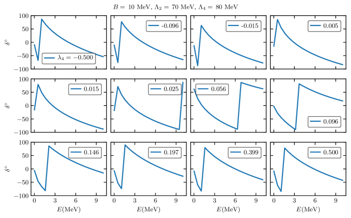
Figure S1: Particle-dimer s-wave scattering phase shift vs. scattering energy $E$ for the nuclear case with $B=10$ MeV, $\Lambda_{2}=70$ MeV and $\Lambda_{4}=80$ MeV.

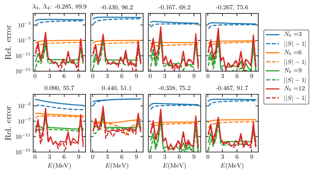
Figure S3: The EC emulator errors for a few test points in the two-dimensional parameter space for the nuclear case with $\Lambda_{2}=75$ MeV. The solid and dashed curves in the same color are the $S$ matrix’s relative errors and the unitarity violation errors respectively with a fixed $N_{b}$ (see the legend).

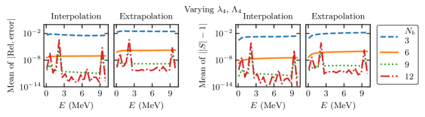
Figure S4: The mean values of the EC emulator errors in the two-dimensional parameter space for the nuclear case with the same training sets as in Fig. S3 (see the legend). $\Lambda_{2}$ is fixed to 75 MeV. The left two panels are the $S$’s relative errors. The right two are the unitarity violation errors. In total, 200 points have been uniformly sampled and tested. The number of interpolation points grows with $N_{b}$. For $N_{b}=12$, the interpolation and extrapolations have similar number of points.

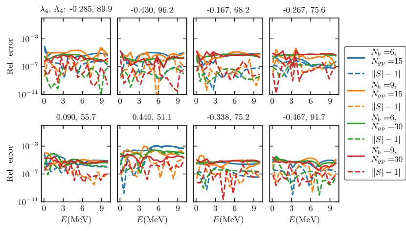
Figure S5: The GP-EC emulator errors for a few test points (the same as those in Fig. S3) in the two-dimensional parameter space for the nuclear case. $\Lambda_{2}=75$ MeV. The emulators implement GP interpolation within the EC emulators. The solid and dashed curves in the same color are the $S$ errors and the unitarity violation errors respectively with a pair of fixed $N_{b}$ and $N_{gp}$ (see the legend).

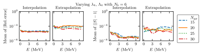
Figure S6: The mean of the GP-EC emulator errors in the two-dimensional parameter space for the nuclear case based on the same 200 points tested in Fig. S4, with $N_{b}=6$ and four different $N_{gp}$. Interpolation vs extrapolation are defined in the same way as in Figs. S4 and 5.

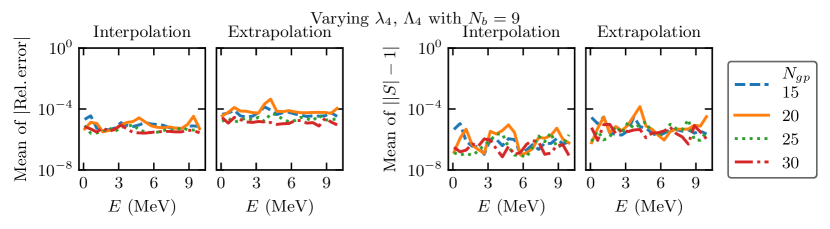
Figure S7: The same as Fig. S6 but with a larger $N_{b}=9$.

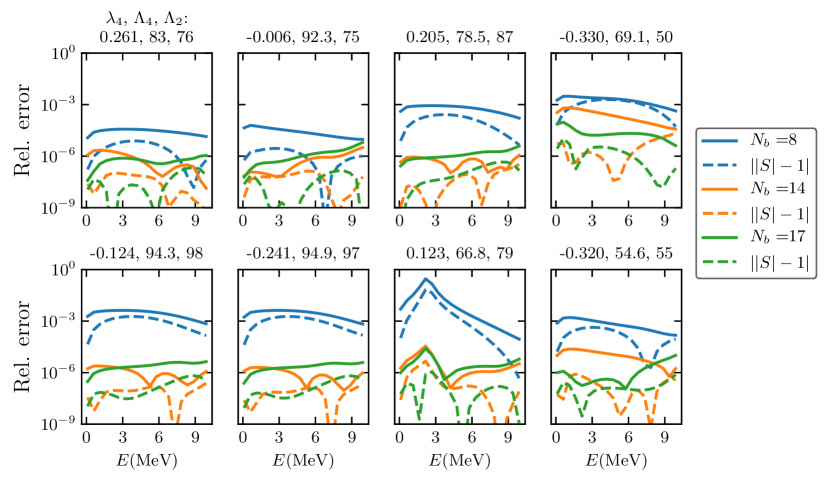
Figure S8: The EC emulator errors for a few test points in the three-dimensional parameter space for the nuclear case with increasing number of $N_{b}$. The solid and dashed curves in the same color are the $S$ matrix’s relative errors and the unitarity violation errors respectively with a fixed $N_{b}$ (see the legend).

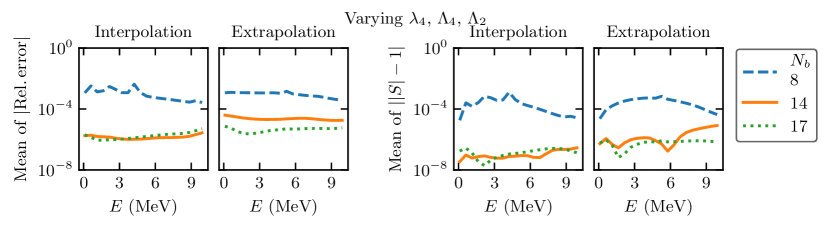
Figure S9: The mean of the EC emulator errors in the three-dimensional parameter space for the nuclear case based on a sample of 1000 test points uniformly sampled in the parameter space. The same three different training sets as in Fig. S8 are used.

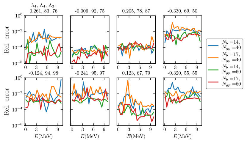
Figure S10: The $S$’s relative errors of the GP-EC emulator for a few test points in the three-dimensional parameter space—the same as those in Fig. S8—for the nuclear case. Four training sets with different combinations of $N_{b}$ and $N_{gp}$ have been shown.

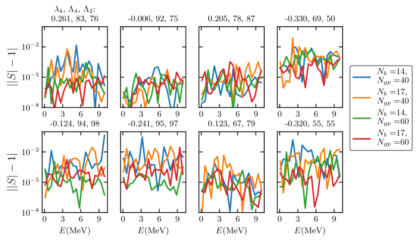
Figure S11: The same as Fig. S10 but for the unitarity violation errors of the GP-EC emulators.

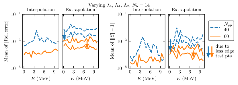
Figure S12: The mean of the GP-EC emulator errors vs $E$ (left two for the $S$ relative errors and the right two for the unitarity violation errors) in the three-dimensionalparameter space for the nuclear case, with $N_{b}=14$ and different $N_{gp}$. Two different calculations are done: the first based on the same 1000 test point sample as used in Fig. S9 with $\Lambda_{2}$ and $\Lambda_{4}$ in $[50,100]$ MeV (266 interpolation and 734 extrapolation points) and the second with $\Lambda_{2}$ and $\Lambda_{4}$ in a smaller $[55,95]$ MeV range (260 interpolation and 380 extrapolation points). As can be seen, reducing the number of the edge test points reduces the errors in the extrapolation sample to a similar level as those in the interpolation sample.

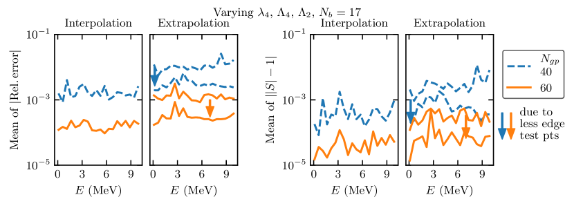
Figure S13: The same as in Fig. S12 but with $N_{b}=17$. For the full sample calculation with $\Lambda_{2}$ and $\Lambda_{4}$ in $[50,100]$ MeV, there are 340 interpolation and 660 extrapolation points, while for the smaller range calculations 328 interpolation and 312 extrapolation points. Similar to Fig. S12, reducing the number of the edge test points reduces the errors in the extrapolation sample to the same level as those in the interpolation sample.

We also explore a second parameter set that mimics the nuclear case with binding energy 10 MeV, with $|\lambda_{4}|\leq 0.5$ and $\Lambda_{2}$ and $\Lambda_{4}$ between $50$ and $100$ MeV. The figures in this section are in parallel to those for the nucleon case in the main text. The results in both cases are qualitatively similar.

References

- Glöckle (1983) W. Glöckle, The Quantum Mechanical Few-Body Problem (Springer-Verlag, Berlin, 1983).
- Gloeckle et al. (1996) W. Gloeckle, H. Witala, D. Huber, H. Kamada, and J. Golak, Phys. Rept. 274, 107 (1996).
- Nielsen et al. (2001) E. Nielsen, D. V. Fedorov, A. S. Jensen, and E. Garrido, Phys. Rep. 347, 373 (2001).
- Deltuva et al. (2014) A. Deltuva, A. C. Fonseca, and R. Lazauskas, Lect. Notes Phys. 875, 1 (2014), arXiv:1201.4979 [nucl-th] .
- Frame (2019) D. K. Frame, Ab Initio Simulations of Light Nuclear Systems Using Eigenvector Continuation and Auxiliary Field Monte Carlo, Ph.D. thesis (2019), arXiv:1905.02782 .
- MacKay (1998) D. J. C. MacKay, in Neural Networks and Machine Learning, NATO ASI Series, Vol. 168, edited by C. M. Bishop (Springer, Berlin, 1998) pp. 133–166.
- Rasmussen and Williams (2006) C. E. Rasmussen and C. K. I. Williams, Gaussian Processes for Machine Learning, Adaptive computation and machine learning series (University Press Group Limited, Cambridge, MA, 2006).
- Bogojeski et al. (2020) M. Bogojeski, L. Vogt-Maranto, M. E. Tuckerman, K.-R. Müller, and K. Burke, Nat. Commun. 11, 5223 (2020).
- Breen et al. (2020) P. G. Breen, C. N. Foley, T. Boekholt, and S. P. Zwart, MNRAS 494, 2465 (2020), arXiv:1910.07291 [astro-ph.GA] .
- König et al. (2020) S. König, A. Ekström, K. Hebeler, D. Lee, and A. Schwenk, Phys. Lett. B 810, 135814 (2020), arXiv:1909.08446 [nucl-th] .
- Ekström and Hagen (2019) A. Ekström and G. Hagen, Phys. Rev. Lett. 123, 252501 (2019), arXiv:1910.02922 [nucl-th] .
- Wesolowski et al. (2021) S. Wesolowski, I. Svensson, A. Ekström, C. Forssén, R. J. Furnstahl, J. A. Melendez, and D. R. Phillips, (2021), arXiv:2104.04441 [nucl-th] .
- Franzke et al. (2021) M. C. Franzke, A. Tichai, K. Hebeler, and A. Schwenk, (2021), arXiv:2108.02824 [nucl-th] .
- Yoshida and Shimizu (2021) S. Yoshida and N. Shimizu, (2021), arXiv:2105.08256 [nucl-th] .
- Furnstahl et al. (2020) R. J. Furnstahl, A. J. Garcia, P. J. Millican, and X. Zhang, Phys. Lett. B 809, 135719 (2020), arXiv:2007.03635 [nucl-th] .
- Melendez et al. (2021) J. Melendez, C. Drischler, A. Garcia, R. Furnstahl, and X. Zhang, Phys. Lett. B 821, 136608 (2021).
- Drischler et al. (2021) C. Drischler, M. Quinonez, P. G. Giuliani, A. E. Lovell, and F. M. Nunes, (2021), arXiv:2108.08269 .
- Epelbaum et al. (2009) E. Epelbaum, H.-W. Hammer, and U.-G. Meißner, Rev. Mod. Phys. 81, 1773 (2009), arXiv:0811.1338 .
- Hebeler (2021) K. Hebeler, Phys. Rept. 890, 1 (2021), arXiv:2002.09548 [nucl-th] .
- King et al. (2019) G. B. King, A. E. Lovell, L. Neufcourt, and F. M. Nunes, Phys. Rev. Lett. 122, 232502 (2019), arXiv:1905.05072 [nucl-th] .
- Eliyahu et al. (2020) M. Eliyahu, B. Bazak, and N. Barnea, Phys. Rev. C 102, 044003 (2020), arXiv:1912.07017 [nucl-th] .
- Zhang et al. (2020a) X. Zhang, S. R. Stroberg, P. Navrátil, C. Gwak, J. A. Melendez, R. J. Furnstahl, and J. D. Holt, Phys. Rev. Lett. 125, 112503 (2020a), arXiv:2004.13575 [nucl-th] .
- Nesbet (1980) R. Nesbet, Variational methods in electron-atom scattering theory, Physics of atoms and molecules (Plenum Press, 1980).
- Bai and Ren (2021) D. Bai and Z. Ren, Phys. Rev. C 103, 014612 (2021), arXiv:2101.06336 [nucl-th] .
- Witala and Gloeckle (2012) H. Witala and W. Gloeckle, Phys. Rev. C 85, 064003 (2012), arXiv:1204.5022 [nucl-th] .
- Pomerantsev et al. (2016) V. N. Pomerantsev, V. I. Kukulin, O. A. Rubtsova, and S. K. Sakhiev, Computer Physics Communications 204, 121 (2016), arXiv:1508.07441 [physics.comp-ph] .
- (27) BUQEYE collaboration, https://buqeye.github.io/software/.
- Rheinboldt (1993) W. C. Rheinboldt, Nonlinear Analysis: Theory, Methods & Applications 21, 849 (1993).
- Chen et al. (2017) P. Chen, A. Quarteroni, and G. Rozza, SIAM/ASA Journal on Uncertainty Quantification 5, 813 (2017).
- Frame et al. (2018) D. Frame, R. He, I. Ipsen, D. Lee, D. Lee, and E. Rrapaj, Phys. Rev. Lett. 121, 032501 (2018), arXiv:1711.07090 .
- Descouvemont (2016) P. Descouvemont, Comput. Phys. Commun. 200, 199 (2016), arXiv:1510.03540 [nucl-th] .
- Faddeev (1960) L. D. Faddeev, Zh. Eksp. Teor. Fiz. 39, 1459 (1960).
- Gignoux et al. (1974) G. Gignoux, A. Laverne, and S. P. Merkuriev, Phys. Rev. Lett. 33, 1350 (1974).
- Lazauskas and Carbonell (2019) R. Lazauskas and J. Carbonell, Few Body Syst. 60, 62 (2019), arXiv:1908.04861 [quant-ph] .
- Alt et al. (1967) E. O. Alt, P. Grassberger, and W. Sandhas, Nucl. Phys. B 2, 167 (1967).
- Watson and Nuttall (1967) K. M. Watson and J. Nuttall, Topics in Several Particle Dynamics (Holden‐Day, Inc., San Francisco, 1967).
- Phillips (1966) A. Phillips, Phys. Rev. 142, 984 (1966).
- Lovelace (1964) C. Lovelace, Phys. Rev. 135, B1225 (1964).
- Thomas (1977) A. W. Thomas, ed., Modern Three Hadron Physics, Vol. 2 (1977) pp. 1–250.
- Kohn (1948) W. Kohn, Phys. Rev. 74, 1763 (1948).
- Kievsky (1997) A. Kievsky, Nucl. Phys. A 624, 125 (1997), arXiv:nucl-th/9706061 .
- Gerjuoy et al. (1983) E. Gerjuoy, A. R. P. Rau, and L. Spruch, Rev. Mod. Phys. 55, 725 (1983).
- Tang (1993) B. Tang, Journal of the American Statistical Association 88, 1392 (1993).
- Baye (2015) D. Baye, Physics Reports 565, 1 (2015), the Lagrange-mesh method.
- GPy (2012) GPy, “GPy: A gaussian process framework in python,” http://github.com/SheffieldML/GPy (since 2012).
- Higdon et al. (2008) D. Higdon, J. Gattiker, B. Williams, and M. Rightley, Journal of the American Statistical Association 103, 570 (2008).
- INT (2021) “Int program 21-1b: Nuclear forces for precision nuclear physics,” https://sites.google.com/uw.edu/int/programs/21-1b (2021).
- Jackura et al. (2019) A. W. Jackura, S. M. Dawid, C. Fernández-Ramírez, V. Mathieu, M. Mikhasenko, A. Pilloni, S. R. Sharpe, and A. P. Szczepaniak, Phys. Rev. D 100, 034508 (2019), arXiv:1905.12007 [hep-ph] .
- Zhang et al. (2020b) X. Zhang, K. M. Nollett, and D. Phillips, J. Phys. G 47, 054002 (2020b), arXiv:1909.07287 [nucl-th] .
- Witała et al. (2021) H. Witała, J. Golak, and R. Skibiński, Eur. Phys. J. A 57, 241 (2021), arXiv:2103.13237 [nucl-th] .
- (51) DLMF, “NIST Digital Library of Mathematical Functions,” http://dlmf.nist.gov/, Release 1.1.0 of 2020-12-15, f. W. J. Olver, A. B. Olde Daalhuis, D. W. Lozier, B. I. Schneider, R. F. Boisvert, C. W. Clark, B. R. Miller, B. V. Saunders, H. S. Cohl, and M. A. McClain, eds.
Supplementary Material for Fast emulation of quantum three-body scattering
Xilin Zhang,1,2 and R. J. Furnstahl 2
1Facility for Rare Isotope Beams, Michigan State University, MI 48824, USA
2Department of Physics, The Ohio State University, Columbus, Ohio 43210, USA