Explainability-Aware One Point Attack for Point Cloud Neural Networks

Abstract

With the proposition of neural networks for point clouds, deep learning has started to shine in the field of 3D object recognition while researchers have shown an increased interest to investigate the reliability of point cloud networks by adversarial attacks. However, most of the existing studies aim to deceive humans or defense algorithms, while the few that address the operation principles of the models themselves remain flawed in terms of critical point selection. In this work, we propose two adversarial methods: One Point Attack (OPA) and Critical Traversal Attack (CTA), which incorporate the explainability technologies and aim to explore the intrinsic operating principle of point cloud networks and their sensitivity against critical points perturbations. Our results show that popular point cloud networks can be deceived with almost $100\%$ success rate by shifting only one point from the input instance. In addition, we show the interesting impact of different point attribution distributions on the adversarial robustness of point cloud networks. Finally, we discuss how our approaches facilitate the explainability study for point cloud networks. To the best of our knowledge, this is the first point-cloud-based adversarial approach concerning explainability. Our code is available at https://github.com/Explain3D/Exp-One-Point-Atk-PC.

1 Introduction

Developments in the field of autonomous driving and robotics have heightened the need for the research of point cloud (PC) data since PC s are advantageous over other 3D representations for real-time performance. However, compared with 2D images, the robustness and reliability of PC networks have only attracted considerable attention in recent years and still not been sufficiently studied, which potentially threatens human lives e.g. driverless vehicles with point cloud recognition systems are unreliable unless they are sufficiently stable and transparent.

Several attempts have been made to investigate the adversarial attacks on PC networks, e.g. [20] and [44]. The first series of approaches (shape-perceptible), represented by [20], although produce geometrically continuous adversarial examples with external generative models, are of limited contribution to the exploration of the classifier itself. Another series (point-shifting) represented by [44] have shown a possibility that moving (dropping or adding) points at crucial positions can successfully fool the classifier. Nevertheless, most of such studies have only focused on minimizing perturbation distances for imperceptibility. Conversely, we start from a different perspective by exploring attacks on PC networks with a minimal number of perturbed points. Additionally, we argue that existing choices of critical points could be further optimized incorporating explainability approaches.

In comparison to previous studies, our work is motivated by the following reasons:

Vicinity of decisions: Minimal perturbation facilitates awareness of the vicinity of the input instances. Although most point-shifting methods also minimize perturbations, they place more emphasis on the perturbation distance and neglect the dimensionality. For high-dimensional decision boundaries, reduction of perturbation dimension is an important way to enhance comprehensibility, which can be regarded as ”cutting the input space using very low-dimensional slices” [33].

Model operating principle: Part of the point-shifting methods also deceived the classifier by perturbing critical points, however, we argue that their selection of critical points is flawed. On the other hand, [14] demonstrated that feature attributions for PC classification networks are extremely sparse, while no work has specifically studied how these attributions are distributed among the critical points as well as their impact on the prediction sensitivity.

Potential for explainability: Another possibility of one-dimensional perturbations is explainability. The explainability method called counterfactuals alters the prediction label by perturbing the input features to provide a convincing explanation to the users. Previous researches have documented that humans are more receptive to counterfactuals with sparse-dimensional perturbations [16, 24, 3]. Incorporating part semantics, Our approach has the potential to be extended for generating high-quality counterfactuals. Moreover, ours require only the access of gradients and no additional generative models, and are therefore more intrinsically explainable.

Altogether, the contribution of this work can be summarized as follows:

• We propose two explainability method-based adversarial attacks: one-point attack (OPA) and critical traverse attack (CTA). Incorporating the attribution from explainable AI, our methods fool the popular PC networks with almost $100\%$ success rate. Supported by extensive experiments, a significant margin is established with existing approaches in terms of the perturbation sparsity.

• We investigate diverse pooling architectures as alternatives to existing point cloud networks, which have an impact on the internal vulnerability against critical points shifting.

• We discuss the research potential of adversarial attacks from an explainability perspective, and present an application of our methods on facilitating the evaluation of explainability approaches.

The rest of the paper is organized as follows: We introduce the related researches of PC attacks in section 2, then we detailed our proposed methods in section 3. In section 4, we present the visualization of the adversarial examples and demonstrate comparative results with existing studies. In section 5 we discuss interesting observations derived from experiments with respect to robustness and explainability. We finally summarize our work in section 6.

2 Related Work

As the first work [37] on adversarial examples was presented, an increasing variety of attacks against 2D image neural networks followed [12, 6, 19, 28, 9, 25]. However, due to the structural distinctions with PC networks (see Supplementary section 7.1.1), we do not elaborate on the attack methods of image deep neural networks (DNN) s. Relevant information about image adversarial examples refers to [2]. It is notable that [33] investigated one-pixel attack for fooling image DNN s and also aimed at exploring the boundary of inputs. Nevertheless, their approach is a black-box attack based on an evolutionary algorithm, which is essentially distinct from ours.

Existing PC attacks are generally categorized into two classes: (i) Shape-perceptible generation, which generates human-recognizable adversarial examples with consecutive surfaces or meshes via generative models or spacial geometric transformations [45, 20, 41, 21, 15, 47, 23, 49]. (ii) Point-shifting perturbation, which regularize the distance or dimension of the point-wise shifting via perturbing or gradient-aware white-box algorithms [17, 48, 42, 44, 34, 22]. Point-wise perturbations, especially gradient-aware attack methodologies, enable more intrinsic explorations of the model properties such as stabilities and decision boundaries. On the other hand, from the perspective of explainability, the majority of generative models contain complex network structures that are inherently unexplainable. Utilizing their output to interpret another model is counter-intuitive.

The conception ”critical points” has been discussed by part of the approaches in (ii) [44, 17, 48, 42] as well as the PointNet proposer [29], which forms the skeletons of the input instances in the classification processes. Existing methods extract the critical points by tracing the ones that remain active from the pooling layer, or by observing the gradient-based saliency maps. While such approaches succeed in generating adversarial examples with minor perturbation distances and sparse shift dimensions, we argue that their modules for selecting critical points can be further optimized. Due to the complex structure of the network, it is difficult to determine whether the surviving points from the pooling layer conclusively make significant contributions to the prediction. Besides, saliency maps based on raw gradients are defective [1, 35]. The above factors may result in the involvement of fake critical points or omission of real ones during the perturbation process, which severely impairs the performance of the adversarial algorithms.

3 Methods

In this section, we formulate the adversarial problem in general and introduce the critical points set (subsection 3.1). We present our new attack approaches (subsection 3.2).

3.1 Problem Statement

Let $P\in\mathbb{R}^{n\times d}$ denotes the given point cloud instance, $f:P\rightarrow y$ denotes the chosen PC neural network and $M(a,b):\mathbb{R}^{n_{a}\times d}\times\mathbb{R}^{n_{b}\times d}$ denotes the perturbation matrix between instance $a$ and $b$. The goal of this work is to generate an adversarial examples $P^{\prime}\in\mathbb{R}^{n^{\prime}\times d}$ which satisfies:

$$argmin( \left|\{m\in M(P,P^{\prime}))|m\neq 0\right\}|$$ (1)

$$+ \left\|M(P,P^{\prime}))\right\|):f(P^{\prime})\neq f(P)$$

Note that among the three popular attack methods for PC data: point adding ($n^{\prime}>n$), point detaching ($n^{\prime}<n$) and point shifting ($n^{\prime}=n$), this work considers point shifting only.

We address the adversarial task in equation 1 as a gradient optimization problem. We minimize the loss on the input PC instance while freezing all parameters of the network:

$$L=\alpha\times Z[f(P)]+\beta\times D(P,P^{\prime})$$ (2)

where $\alpha$ indicates the optimization rate, $Z[f(P)]$ indicates the neuron unit corresponding to the prediction $f(P)$ which guaranties the alteration of prediction, $D(P,P^{\prime})$ represents the quantized imperceptibility between the input $P$ and the adversarial example $P^{\prime}$ and $\beta$ is the distance penalizing weight. The imperceptibility has two major components, namely the perturbation magnitude and the perturbation sparsity. The perturbation magnitude can be constrained in three ways: Chamfer distance (equation 3), Hausdorff distance (equation 4) or simply Euclidean distance. We ensure perturbation sparsity by simply masking the gradient matrix, and with the help of the saliency map derived by the explainability method we only need to shift those points that contribute positively to the prediction to change the classification results, which are termed as ”critical points set”.

Critical points set: The concept was first discussed by its proposer [29], which contributes to the features of the max-pooling layer and summarizes the skeleton shape of the input objects. They demonstrated an upper-bound construction and proved that corruptions falling between the critical set and the upper-bound shape pose no impact on the predictions of the model. However, the impairment of shifting those critical points is not sufficiently discussed. Previous adversarial researches studied the model robustness by perturbing or dropping critical points set identified through monitoring the max-pooling layer or accumulating loss of gradients [44, 17, 48, 42]. Nevertheless, capturing the output of the max-pooling layer struggles to identify the real critical points set due to the lack of transparency in the high-level structures (e.g., multiple MLPs following the pooling layer), while saliency maps based on raw gradients suffer from saturation [1, 35], both of which severely compromise the filtering of the critical point set. We therefore introduce Integrated Gradients (IG) [36], the state-of-the-art gradient-based explainability approach, to further investigate the sensitivity of model robustness to the critical points set. The formulation of IG is summarized in equation S1.

Similarity metrics for point cloud data: Due to the irregularity of PC s, Manhattan and Euclidean distance are both no longer applicable when measuring the similarity between PC instances. Several previous works introduce Chamfer [17, 46, 44, 20, 23, 49, 45] and Hausdorff [50, 17, 46, 44, 23, 49] distances to represent the imperceptibility of adversarial examples. The measurements are formulated as:

• Bidirectional Chamfer distance

  $$D_{c}(P_{a},P_{b})= \frac{1}{|P_{a}|}\sum_{p_{m}\in P_{a}}\min_{p_{n}\in P_{b}}\left\|p_{m}-p_{n}\right\|_{2}+$$ (3)

  $$\frac{1}{|P_{b}|}\sum_{p_{n}\in P_{b}}\min_{p_{m}\in P_{a}}\left\|p_{n}-p_{m}\right\|_{2}$$

• Bidirectional Hausdorff distance

  $$D_{h}(P_{a},P_{b})=\max( \max(\min_{p_{n}\in P_{b}}\left\|p_{m}-p_{n}\right\|_{2}),$$ (4)

  $$max(\min_{p_{m}\in P_{a}}\left\|p_{n}-p_{m}\right\|_{2}))$$

3.2 Attack Algorithms

One-Point Attack (OPA): Specifically, OPA (see Supplementary algorithm 1 for pseudo-code) is an extreme of restricting the number of perturbed points, which requires:

$$\left|\{m\in M(P,P^{\prime}))|m\neq 0\right\}|=1$$ (5)

We acquire the gradients that minimize the activation unit corresponding to the original prediction, and a saliency map based on the input PC instance from the explanation generated by IG. We sort the saliency map and select the point with the top-$n$ attribution as the critical points ($n=1$ for OPA), and mask all points excluding the critical one on the gradients matrix according to its index. Subsequently the critical points are shifted with an iterative optimization process. An optional distance penalty term can be inserted into the optimization objective to regularize the perturbation magnitude and enhance the imperceptibility of the adversarial examples. We choose Adam [18] as the optimizer, which has been proven to perform better for optimization experiments. The optimization process may stagnate by falling into a local optimum, hence we treat every $25$ steps as a recording period, and the masked Gaussian noise weighted by $W_{n}$ is introduced into the perturbed points when the average of the target activation at period $k+1$ is greater than at period $k$. For the consideration of time cost, the optimization process is terminated when certain conditions are fulfilled and the attack to the current instance is deemed as a failure.

Critical Traversal Attack (CTA): Due to the uneven vulnerability of different PC instances, heuristically setting a uniform sparsity restriction for the critical points perturbation is challenging. CTA (pseudo-code presented in Supplementary algorithm 2) enables the constraint of perturbation sparsity to be adaptive by attempting the minimum number of perturbed points for each instance subject to a successful attack. The idea of CTA is starting with the number of perturbed points $n$ as $1$ and increasing by $1$ for each local failure until the prediction is successfully attacked or globally failed. Similarly, we consider the saliency map generated by IG as the selection criterion for critical points, and the alternative perturbed points are incremented from top-$1$ to all positively attributed points. Again, for accelerating optimization we also select Adam [18] as the optimizer. Since most PC instances can be successfully attacked by one-point shifting through the introduction of Gaussian noise in the optimization process, we discarded the noise-adding mechanism in CTA to distinguish the experiment results from OPA. The aforementioned local failure stands for terminating the current $n$-points attack and starting another $n+1$ round, while the global failure indicates that for the current instance the attack has failed. We detail the stopping criteria for OPA and CTA in section 7.2.2.

4 Experiments

In this section, we present and analyze the results of the proposed attack approaches. We demonstrate quantitative adversarial examples in subsection 4.1 and scrutinize the qualitative result in subsection 4.2. Our experiments were primarily conducted on PointNet [29], which in general achieves an overall accuracy of $87.1\%$ for the classification task on ModelNet40 [43]. Moreover, we also extended our approaches to attack the most popular PC network PointNet++ [30] and DGCNN [40], which dominate the PC classification task with $90.7\%$ and $92.2\%$ accuracies respectively. We choose Modelnet40 [43] as the experimental dataset, which contains $12311$ CAD models ($9843$ for training and $2468$ for evaluation) from $40$ common categories, and is currently the most widely-applied point cloud classification dataset. We randomly sampled $25$ instances for each class from the test set, and then selected those instances that are correctly predicted by the model as our victim samples. We also validate our methods on ShapeNet [7] dataset. All attacks performed in this section are non-targeted unless specifically mentioned. In all experiments, we only compare the performances among point-shifting attacks, motivated by exploring the peculiarities of PC networks. Though previous shape-perceptible approaches such as [47, 15, 49, 20, 45] also addressed adversarial studies of PC s, they were devoted to generate adversarial instances with human-perceptible geometries. Comparison of perturbation distances and dimensions with their works is not relevant, and therefore we do not consider them as competitors.

4.1 Adversarial examples visualization

Fig. 1 visualizes two adversarial examples for OPA and CTA respectively. Interestingly, in CTA, regardless of the absence of the restriction on the perturbation dimension, there are instances (e.g. the car in CTA) where only one-point shifting is required to generate an adversarial example. More qualitative visualizations are presented in Fig. S1 and S2.

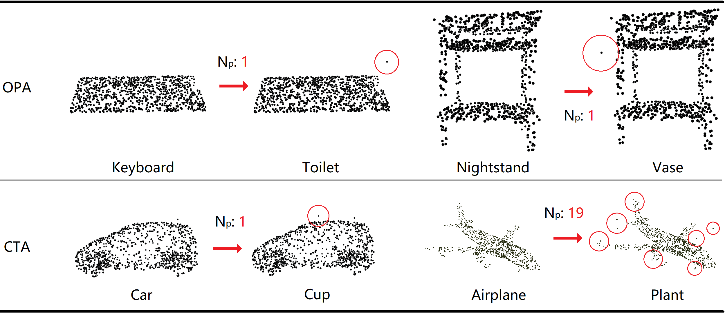
Figure 1: Adversarial examples for OPA and CTA. $N_{p}$ denotes how many points are shifted.

4.2 Quantitative evaluations and comparisons

In this section, we compare the imperceptibility of proposed methods with existing attacks via measuring Hausdorff and Chamfer distances as well as the number of shifted points, and demonstrate their transferability among different popular PC networks. Additionally, we show that CTA maintains a remarkably high success rate even after converting to targeted attacks.

Imperceptibility: We compare the quality of generated adversarial examples with other point-shifting researches under the aspect of success rate, Chamfer and Hausdorff distances, and the number of points perturbed. As table 1 shows, compared to the approaches favoring to restrict the perturbation magnitude, despite the relative laxity in controlling the distance between the adversarial examples and the input instances, our methods prevail significantly in terms of the sparsity of the perturbation matrix. Simultaneously, our methods achieve a higher success rate, implying that the network can be fooled for almost all PC instances by shifting a minuscule amount of points (even one). In the experiment, the optimization rate $\alpha$ is empirically set to $10^{-6}$, which performs as the most suitable step size for PointNet after grid search. Specifically for OPA, we set the Gaussian weight $W_{n}$ to $10^{-1}$, which proved to be the most suitable configuration. More analytical results of different settings of $\beta$ and $W_{n}$ is demonstrated in Fig. S5. Note that while calculating $D_{c}$ and $D_{h}$, we employ the L2-norm. Therefore, despite the large Hausdorff distance, the average perturbation magnitude along each axis is $\bm{0.488}$. Considering that each axis of ModelNet40 is regularized into the interval $[-1,1]$, this magnitude occupies $\bm{24.4\%}$ of the interval, which corresponds to an average perturbation of $62.2$ gray values in 2D grayscale images. We thus consider the perturbation magnitude to be acceptable.

To eliminate potential bias, we also test the proposed attack methods with ShapeNet [7] dataset. As table 2 presents, our approaches perform similarly on the two different datasets, and therefore the vulnerable bias in the data distribution of ModelNet40 can be basically excluded.

	S	$D_{c}$	$D_{h}$	$N_{p}$
$L_{p}$ Norm [44]	$85.9$	$1.77\times 10^{-4}$	$2.38\times 10^{-2}$	$967$
Minimal selection [17]	$89.4$	$1.55\times 10^{-4}$	$1.88\times 10^{-2}$	$36$
Adversarial sink [23]	$88.3$	$7.65\times 10^{-3}$	$1.92\times 10^{-1}$	1024
Adversarial stick [23]	$83.7$	$4.93\times 10^{-3}$	$1.49\times 10^{-1}$	210
Random selection [42]	$55.6$	$7.47\times 10^{-4}$	$2.49\times 10^{-3}$	413
Critical selection [42]	$19.0$	$1.15\times 10^{-4}$	$9.39\times 10^{-3}$	50
Critical frequency [48]	$63.2$	$5.72\times 10^{-4}$	$2.50\times 10^{-3}$	303
Saliency map/L [48]	$56.0$	$6.47\times 10^{-4}$	$2.50\times 10^{-3}$	358
Saliency map/H [48]	$58.4$	$7.52\times 10^{-4}$	$2.48\times 10^{-3}$	424
Ours (OPA)	$98.7$	$8.64\times 10^{-4}$	$8.45\times 10^{-1}$	$1$
Ours ($\lx@glossaries@gls@link{acronym}{cta}{\leavevmode\textsc{CTA}}_{\beta=0}$)	$100$	$8.92\times 10^{-4}$	$8.19\times 10^{-1}$	$2$
Ours ($\lx@glossaries@gls@link{acronym}{cta}{\leavevmode\textsc{CTA}}_{\beta=1e-3}$)	$99.6$	$7.73\times 10^{-4}$	$6.68\times 10^{-1}$	$6$

Table 1: Comparison of existing point-shifting adversarial generation approaches for PointNet, where $S$, $D_{c}$, $D_{h}$ and $N_{p}$ denote the success rate, Chamfer and Hausdorff distances and the number of shifted points respectively. Part of the records sourced from [17]. It is worth noting that we only compare the gradient-based point-shifting competitors.

	Dataset	S	$D_{c}$	$D_{h}$	$N_{p}$
OPA	ModelNet40	$98.7$	$8.64\times 10^{-4}$	$8.45\times 10^{-1}$	$1$
	ShapeNet	$95.1$	$8.39\times 10^{-4}$	$8.06\times 10^{-1}$	$1$
CTA	ModelNet40	$100$	$8.92\times 10^{-4}$	$8.19\times 10^{-1}$	$2$
	ShapeNet	$100$	$8.91\times 10^{-4}$	$7.26\times 10^{-1}$	$3$

Table 2: Comparison of attack results with ModelNet40 and ShapeNet dataset.

In addition to PointNet, we also tested the performance of our proposed methods on PC networks with different architectures. Table 3 summarize the result of attack PointNet, PointNet++ and DGCNN with both OPA and CTA respectively. Surprisingly, these state-of-the-art PC networks are vulnerable to the one-point attack with remarkably high success rates. On the other hand, CTA achieves almost $100\%$ success rate fooling those networks while only a single-digit number of points are shifted. Intuitively, PC neural networks appear to be more vulnerable compared to image CNNs ([33] is a roughly comparable study since they also performed one-pixel attack with the highest success rate of $71.66\%$) (see table S1 and Fig. S7 in supplementary for results of OPA). An opposite conclusion has been drawn by [44], they trained the PointNet with 2D data and compared its robustness with 2D CNNs against adversarial images. Nevertheless, we argue that the adversarial examples are generated by attacking a 2D CNN, such attacks may not be aggressive for PointNet, which is specifically designed for PC s.

	Model	S	$D_{c}$	$D_{h}$	$N_{p}$
O P A	PN	$98.7$	$\bm{8.45\times 10^{-4}}$	$\bm{8.64\times 10^{-1}}$	$1$
	PN++	$\bm{99.1}$	$1.58\times 10^{-2}$	$1.61\times 10^{1}$	$1$
	DGCNN	$90.9$	$1.70\times 10^{-3}$	$1.69$	$1$
C T A	PN	$\bm{100}$	$\bm{8.92\times 10^{-4}}$	$\bm{8.19\times 10^{-1}}$	$6$
	PN++	$99.5$	$1.22\times 10^{-2}$	$8.90$	$6$
	DGCNN	$100$	$2.13\times 10^{-3}$	$1.48$	$\bm{3}$

Table 3: Comparison of attack results on PN(PointNet), PN++(PointNet++) and DGCNN.

Transferability: We further investigate the transferability of proposed attacks across different PC networks by feeding the adversarial examples generated by one network to the others and recording the overall classification accuracy. Fig. 2 presents the adversarial transferability between PointNet, PointNet++ and DGCNN. What stands out in the figure is that PointNet++ and DGCNN show strong stability against the adversarial examples from PointNet. Surprisingly, PointNet++ performs stably against adversarial examples from DGCNN, while the opposite fails. We believe this is because the aggregated adjacency features disperse the attribution of a single point. Recall the EdgeConv [40] in DGCNN, which extracts adjacent features in both point and latent spaces, while PointNet++ possesses a similar module that aggregates neighboring points [29], which can be considered as a point-space-only EdgeConv. Such an integration distributes the feature contribution to multiple adjacent points, and a modest shifting of one point has limited impacts on the aggregated cluster. The feature extractor in PointNet can also be regarded as a special EdgeConv with $K=1$, preserving the location information of the central point only, and therefore is more sensitive to the perturbation. On the other hand, we consider the best stability of PointNet++ stems from the multi-scale(resolution) grouping, where latent features are concatenated by grouping layers at different scales, resulting in more points involved in the aggregation. In section 5.2, we perform a preliminary validation of our conjecture on PointNet.

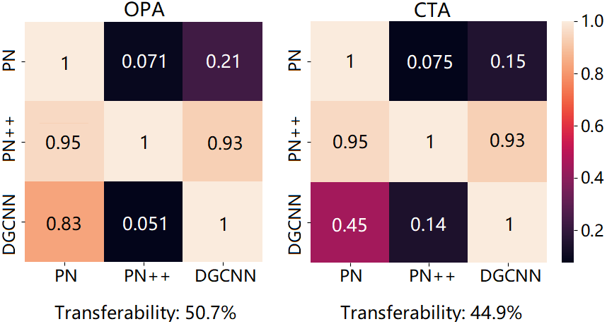
Figure 2: Transferability for PointNet, PointNet++ and DGCNN for OPA (left) and CTA (right). Networks on the rows and columns denote from which victim networks the adversarial examples are generated and to which those examples are transferred respectively. Brighter squares denote higher transferabilities. The total transferabilities under the matrices are the averages of the off-diagonal values of corresponding methods.

Targeted attack: We also extend the proposed methods to targeted attacks. To alleviate redundant experiment procedures, we employ three alternatives of conducting ergodic targeted attack: random, lowest and second-largest activation attack. In the random activation attack we choose one stochastic target from the $39$ labels (excluding the ground-truth one) as the optimization destination. In the lowest and second-largest activation attack, we decrease the activation of ground truth while boosting the lowest or second-largest activation respectively until it becomes the largest one in the logits. The results, as shown in table 4, indicate that though the performance of OPA is deteriorated when converting to targeted attacks due to the rigid restriction on the perturbation dimension, CTA survived even the worst case (the lowest activation attack) with a remarkably high success rate and a minuscule number of perturbation points. We also demonstrate the results from LG-GAN [49], which also dedicates to targeted attack for PC networks. In comparison, CTA achieves an approximated success rate with a much smaller $D_{c}$. Note that their approach is based on generative models and the comparison is for reference only.

	Pattern	S	$D_{c}$	$D_{h}$	$N_{p}$
O P A	Second-largest	58.5	$9.49\times 10^{-4}$	$9.33\times 10^{-1}$	1
	Random	20.9	$1.06\times 10^{-2}$	$1.08\times 10^{1}$	1
	Lowest	6.3	$4.73\times 10^{-3}$	4.80	1
C T A	Second-largest	99.5	$1.55\times 10^{-3}$	$8.14\times 10^{-1}$	5
	Random	97.7	$5.75\times 10^{-3}$	2.31	10
	Lowest	99.0	$8.52\times 10^{-3}$	3.06	13
LG-GAN [49]		98.3	$3.80\times 10^{-2}$	-	-

Table 4: Targeted OPA and CTA on PointNet. Targeting all labels for each instance in the test set is time-consuming. Therefore, we generalize it with three substitutes: random, the second-largest and the lowest activation in the logits. We also show the results of LG-GAN as a reference.

5 Discussion

In this section, we present the relevant properties of PC networks in the maximization activation experiment (5.1) as well as our viewpoint concerning the robustness of PC networks (5.2) and discuss the investigative potential of OPA for PC neural networks from the viewpoint of explainability (5.3).

5.1 Maximized activation

Activation Maximization (AM), first proposed by [11], sets out to visualize a global explanation of a given network through optimizing the input matrix $x$ while freezing all parameters $\theta$ such that the selected $i^{th}$ activation neuron at $l^{th}$ layer $S_{i}^{l}$ is maximized [27]:

$$x^{*}=\underset{x}{\mathrm{argmax}}\,(a_{i}^{l}(\theta,x))$$ (6)

The proposed OPA was motivated by a fruitless AM attempt for PC networks. Fig. 3 displays an example from $1000$-steps AM results of PointNet. More examples with different initializations are depicted in Fig. S8. We conduct the AM experiments with various initializations including zero, point cluster generated by averaging all test data [26] and a certain instance from the class ”Car”. What stands out in the visualization is that the gradient ascent of the PC neural network’s activations appears to depend solely on the magnitude of the outward extension subject to the extreme individual points (the middle figure). We further investigate the explanations of the AM generations utilizing IG and the analysis reveals that almost all the positive attributions are concentrated on the minority points that were expanded (the right figure). Fig. 4 provides a quantitative view of how target activation ascends with the shifting of input points and we introduce Gini coefficient [10] to represent the ”wealth gap” of the Euclidean distance among all points. Interestingly, as the target activation increments over the optimization process, the Gini coefficient of Euclidean distances steepens to $1$ within few steps, indicating that the fastest upward direction of the target activation gradient corresponds with the extension of a minority of points.

	Acc.	S	$D_{c}$	$D_{h}$	$N_{pos}$	Gini.
Max-pooling	87.1	98.7	$8.45\times 10^{-4}$	$8.64\times 10^{-1}$	397.2	$0.91$
Average-pooling	83.8	44.8	$2.94\times 10^{-3}$	$2.96$	718.5	$0.53$
Median-pooling	74.5	0.9	$1.28\times 10^{-4}$	$9.55\times 10^{-2}$	548.1	$0.57$
Sum-pooling	76.7	16.7	$2.50\times 10^{-3}$	$2.53$	868.2	$0.49$

Table 5: Model accuracies, success attacking rates, average Chamfer and Hausdorff distances of OPA on PointNet with max, average, median and sum-pooling on the last layer respectively. The evaluation accuracy is also presented in the second column. $N_{pos}$ denotes how many points are positively attributed to the prediction, and Gini. denotes the Gini coefficient of the corresponding attribution distributions.

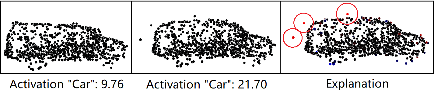
Figure 3: AM results initialized with a certain instance. The first, second and third columns demonstrate the initialized set of points, the AM output results after $1000$ optimization steps and the salience map explanation of the corresponding output explained by IG, respectively. In the explanation, red points indicate the degree of positive attributions.

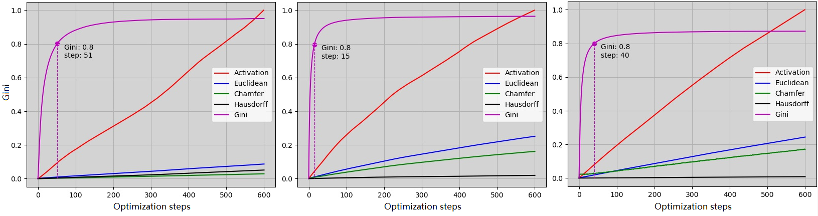
Figure 4: Correlation between the ascending target activation and the various distances of the optimized example from the original initializations: zero (left), the average of the test set (middle) and a certain instance (right). Activations are normalized in order to be visible together with other factors. X-axis denotes the optimization steps and y-axis denotes corresponding values in the legend. The marked points are the steps in the optimization process where the Gini coefficient of the attribution first reaches $0.8$.

5.2 Structural stability of PC networks

Plenty of researches have discussed defense strategies against intentional attacks for PC networks [46, 22, 50, 23, 17, 34, 49, 45], the majority of which were with respect to embedded defense modules, such as outlier removal. However, there has been little discussion about the stability of the intrinsic architectures for PC networks. Inspired by [34] who investigated the impacts of different pooling layers on the robustness, we replace the max-pooling in PointNet with multifarious pooling layers. As table 5 shows, although PointNet with average and sum-pooling sacrifice $3.3\%$ and $10.4\%$ accuracies in the classification task, the success rates of OPA on them plummet from $98.7\%$ to $44.8\%$ and $16.7\%$ respectively, and the requested perturbation magnitudes are dramatically increased, which stands for enhanced stabilization. We speculate that it depends on how many points from the input instances the model employs as bases for predictions. We calculate the normalized IG contributions of all points from the instances correctly predicted among the $2468$ test instances, and we also introduce the Gini coefficient [10] to quantify the dispersion of the absolute attributions which is formulated as:

$$G=\frac{\sum_{i=1}^{n}\sum_{j=1}^{n}\left|\left|a_{i}\right|-\left|a_{j}\right|\right|}{2n^{2}\left|\bar{a}\right|}$$ (7)

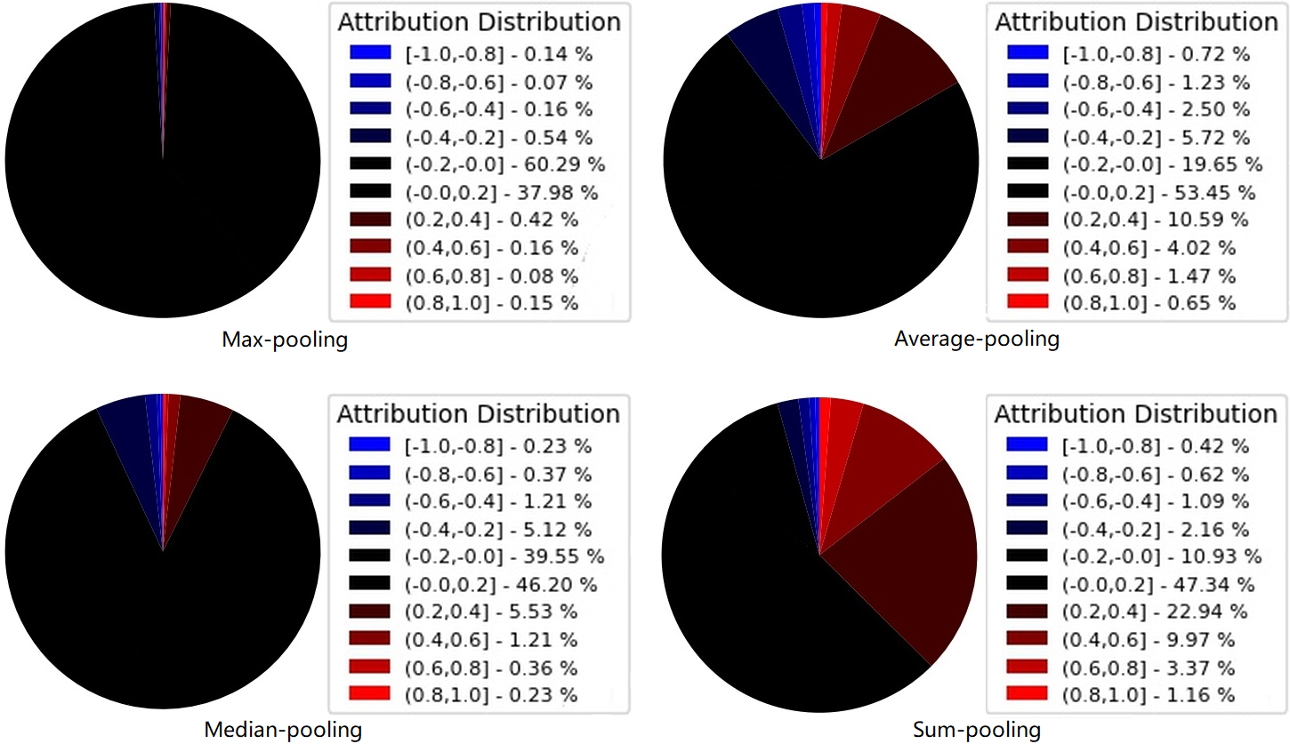
Figure S9: The distributions of attributed points of PointNet structured with max, average, median and sum-pooling layers as the global feature extraction layer respectively.

where $a$ is the attribution mask generated by IG. We demonstrate the corresponding results in table 5, 6 and Fig. S9. There are significant distributional distinctions between the max, average and sum-pooling architectures. PointNet with average and sum-poolings adopt $70.18\%$ ($718.5$ points) and $84.78\%$ ($868.2$ points) of the points to positively sustain the corresponding predictions, where the percentages of points attributed to the top $20\%$ are $0.65\%$ ($6.7$ points) and $1.16\%$ ($11.9$ points), respectively, while these proportions are only $38.79\%$ ($397.2$ points) and $0.15\%$ ($1.5$ points) in the max-pooling structured PointNet. Moreover, the Gini coefficients reveal that in comparison to the more even distribution of attributions in average ($0.53$) and sum-pooling ($0.49$), the dominant majority of attributions in PointNet with max-pooling are concentrated in a minuscule number of points ($0.91$). Hence, it could conceivably be hypothesized that for PC networks, involving and apportioning the attribution across more points in prediction would somewhat alleviate the impact of corruption at individual points on decision outcomes, and thus facilitate the robustness of the networks. Surprisingly, median-pooling appears to be an exception. While the success rate of OPA is as low as $0.9\%$, the generated adversarial examples only require perturbing $9.55\times 10^{-2}$ of the Hausdorff distance in average (all experiments sharing the same parameters, i.e. without any distance penalty attached). On the other hand, despite that merely $53.53\%$ ($548.1$) points are positively attributed to the corresponding predictions, with only $0.23\%$ ($2.4$ points) of them belonging to the top $20\%$, which is significantly lower than the average and sum-pooling architectures, median-pooling is almost completely immune to the deception of OPA. We believe that median-pooling is insensitive to extreme values, therefore the stability to perturbations of a single point is dramatically reinforced.

	Top $20\%$	Top $40\%$	Positive
Max-pooling	$0.15\%$	$0.23\%$	$38.79\%$
Average-pooling	$0.65\%$	$2.12\%$	$70.18\%$
Median-pooling	$0.23\%$	$0.59\%$	$53.53\%$
Sum-pooling	$1.16\%$	$4.53\%$	$84.78\%$

Table 6: Overview of the percentage of top-$20\%$, top-$40\%$ and positive attributed points with four different pooling layers. Complete pie diagrams are shown in Fig. S9.

5.3 Towards explainable PC models

Despite the massive number of adversarial methods that have made significant contributions to the studies of model robustness for computer vision tasks, to our best knowledge, none has discussed the explainability of PC networks. However, we believe that the adversarial methods can facilitate the explainability of the models to some extent. Recall the roles of counterfactuals in investigating the explainability of models processing tabular data [5]. Counterfactuals provide explanations for chosen decisions by describing what changes on the input would lead to an alternative prediction while minimizing the magnitude of the changes to preserve the fidelity, which is identical to the process of generating adversarial examples [8]. Unfortunately, owing to the multidimensional geometric information that is unacceptable to the human brain, existing image-oriented approaches addressed the counterfactual explanations only at the semantic level [13, 39].

Several studies have documented that a better explanatory counterfactual needs to be sparse because of the limitations on human category learning [16] and working memory [24, 3]. Therefore we argue that unidimensional perturbations contribute to depicting relatively perceptible decision boundaries. Fig. 5 compares the visualization of multidimensional and unidimensional perturbations. The unidimensional shift, though larger in magnitude, shows more clearly the perturbation process of the prediction from ”car” to ”radio”, and makes it easier to perceive the decision boundary. Conversely, while higher dimensional perturbations perform better on imperceptibility for humans, they are more difficult for understanding the working principles of the model.

In addition, we find another interesting application of the proposed approaches regarding explainability. Evaluating explanations has long been a major challenge for explainability studies due to the lack of ground truth [4]. An intuitive idea is sensitivity testing, i.e., perturbing features in the explanation that possess high attributions and observing whether the prediction results dramatically change. Theoretically, in our methods, a more accurate explanation induces a more precise selection of critical points, and therefore a higher success rate when perturbing them for generating adversarial examples. Table 7 presents the attack performances utilizing gradient-based explainability methods: Vanilla Gradients [31], Guided Back-propagation [32] and IG as the critical identifier respectively. Our results are consistent with [14] and [38], the performance of IG is comparatively better than that of Vanilla Gradients and Back-propagation.

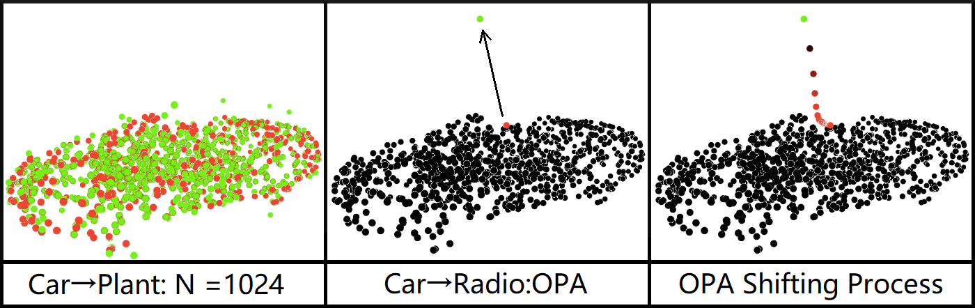
Figure 5: Intuitive visualization of multidimensional shifting(left), unidimensional OPA shifting(middle) and the shifting process of OPA. The redder the point the higher the prediction score for the label ”car”. Green points denote the shifting destinations.

Exp. Med.	S	$D_{c}$	$D_{h}$	$N_{p}$
VG	$82.5$	$8.20\times 10^{-4}$	$8.01\times 10^{-1}$	1
GB	$83.4$	$8.21\times 10^{-4}$	$8.02\times 10^{-1}$	1
IG	$\bm{98.7}$	$8.64\times 10^{-4}$	$8.45\times 10^{-1}$	1

Table 7: OPA performances utilizing various gradient-based explainability methods to identify the critical points, where VG, GB and IG denote Vanilla Gradients [31], Guided Back-propagation [32] and Integrated Gradients respectively.

6 Conclusion

As the first attack methods for PC networks incorporating explainability, though our approaches are easily filtered by defense modules (such as outlier removal, see section 7.9) due to the relatively large perturbation distances, we demonstrate the significance of individual critical points for PC network predictions. We also discussed our viewpoints to the robustness of PC networks as well as their explainability. In future investigations, it might be possible to distill existing PC networks according to the critical points into more explainable architectures. Besides, we are looking forward to higher-quality and human-understandable explanations for PC networks.

7 Supplementary Material

This section is a supplement for the main part of the paper. In this section, we detail additional formulas for the backgrounds (7.1), demonstrate our Pseudo-codes and stopping criteria (7.2), show more adversarial examples for both OPA and CTA respectively (7.3), visualize the diversity of attacking labels (7.4), discuss the most appropriate hyper-parameter settings (7.5). We also present the attack result OPA on 2D images as a comparable reference (7.6). Finally, we provide more visualisations of the Activation Maximization (AM) and the attribution distribution of PC networks (7.7 and 7.8 respectively.)

7.1 Background

7.1.1 Point cloud deep neural networks

A PC input can be represented as $P=\left\{p_{0},...,p_{n}\right\}$, where $p_{i}\in\mathbb{R}^{3}$ and $n$ is the number of component points. Compared with 2D images, the structural peculiarity of PC data lies in the irregularity: let $R(S)$ be a function that randomly disrupts the order of the sequence $S$, a PC classifier $f$ must possess such properties: $f(P)=f(R(P))$, which is regarded as a ”symmetric system”. The pioneer of PC networks is proposed by [29], succeeded by employing an symmetric function $g(S)$ and an element-wise transformer $h(p)$ where $f(P)\approx g(\left\{h(p_{0}),...,h(p_{n})\right\})$ (in their experiments a max-pooling is choosen as $g(S)$). PointNet++ [30], the successor of PointNet, further coalesced hierarchical structures by introducing spatial adjacency via grouping of nearest-neighbors. DGCNN [40] extended the the predecessors by dynamically incorporating graph relationships between multiple layers. All of the point-based methods achieve satisfactory accuracies on acknowledged PC dataset such as ModelNet40 [43].

7.1.2 Integrated Gradients

Gradients-based explainability methods are oriented on generating saliency maps of inputs by calculating gradients during propagation. While vanilla gradients severely suffer from attribution saturation [35],  [36] proposes IG which accumulates attributions from an appropriate baseline before the gradients reach the saturation threshold. IG is formulated as:

$$IG_{i}=(x_{i}-x_{i}^{\prime})\cdot\int_{\alpha=0}^{1}\frac{\partial F(x^{\prime}+\alpha(x-x^{\prime}))}{\partial x}d\alpha$$ (S1)

Where $x^{\prime}$ denotes the given baseline.

7.1.3 Targeted vs. Untargeted attack

For a given classifier $f$ and its logits $a$, an PC input instance $P$ and an adversarial perturbation $A_{p}$:

• Targeted attack

  $$\textrm{Minimize}\quad(a[f(P)+A_{p}])\quad\textrm{s.t.}\quad f(P+A_{p})\neq f(P)$$ (S2)

• Untargeted attack

  $$\textrm{Maximize}\quad(a[f(P+A_{p})])\quad\textrm{s.t.}\quad f(P+A_{p})=T$$ (S3)

  Where $T$ is the given target class.

7.2 Other implementation details

7.2.1 Pseudo-codes of OPA and CTA

In this section we present the Pseudo-codes for both OPA and CTA as a supplement for section 3.2.

7.2.2 Stopping Criteria

Theoretically, CTA can keep searching until all positively contributed points are traversed. For algorithmic efficiency, we set specific stopping criteria for OPA and CTA.

OPA: With the introduction of Gaussian random noise for OPA, the optimization process may fall into an everlasting convergence-noise addition loop, a manually configured failure threshold is therefore essential. A recorder $R_{a}$ is built to record the corresponding prediction activation for each period. We set a global maximum iterations $I_{maxg}$. The stopping criterion of OPA is fulfilled when

• $I_{cur}>I_{maxg}$ or $((Mean(R_{a}^{k+1})>Mean(R_{a}^{k})$ and $Var(R_{a}^{k})\rightarrow 0))$.

Due to the introduction of random Gaussian noise, the optimization process will not fail until the target activation has no fluctuant reaction to the Gaussian noise.

CTA: There are both local and global stopping criteria for CTA. Local criterion stands for terminating the current $N_{p}$ perturbed points and start the $N_{p}+1$ round, which is similar with OPA. Again, we set an activation recorder $R_{a}$ and a local maximum iterations $I_{maxl}$. The local stopping criterion is fulfilled when:

• $I_{cur}>I_{maxl}$ or $Mean(R_{a}^{k+1})>Mean(R_{a}^{k})$

Global stopping terminates the optimization of the current instance and registers it as ”failed”. CTA is designed to shift all the positively attributed points $N_{pos}$ in the worst case which is extremely time-consuming. For practical feasibility, we specify the global maximum iterations $I_{maxg}$. The global stopping criterion for CTA is fulfilled when:

• $I_{cur}>I_{maxg}$ or $N_{p}\geqslant N_{pos}$

where $N_{pos}$ is the total amount of positive attributed points according to the explanation provided by IG.

Input: $P\rightarrow N\times D$ PC data, $f\rightarrow$ PC neural network, $\alpha\rightarrow$ Optimizing rate, $\beta\rightarrow$ Weight for constrain the perturbing distance(optional), $D\rightarrow$ Distance calculating function(optional), $N_{p}\rightarrow$ Number of shifting points($1$ for One-point attack), $W_{n}\rightarrow$ Gaussian noise weights

Output: $P_{adv}\rightarrow N\times D$ Adversarial example

1

$A_{idx}=Argsort(IG(P,f))$

  // Get IG mask of P

2

$R_{s}=list()$

  // Activation Recorder

3

$I_{cur}=1$

  // Current iteration

4

5while True do

       $a_{p}\leftarrow f(P)$

        // Current activation of predicted class

6      

      $G=\alpha*A_{p}+\beta*D(P_{adv},P)$

        // Add distance constrain(Optional)

7      

      $P_{adv}=Adam(P_{adv},G[A_{idx}[1:N]])$

        // Adam optimizing N points

8      

9      $I_{cur}\mathrel{{+}{=}}1$

10      $R_{s}.append(a_{p})$

      /* Add masked Gaussian random noise if activation descending stopped */

11       if $R_{s}[t]<R_{s}[t+1]$  then

12             $P_{adv}\mathrel{{+}{=}}W_{n}\times GaussianRandom(P_{\delta})[A_{idx}[1:N]]$

      /* Success if predict class changed */

13       if $max(a)!=pred$ then

14             return $P_{adv}$

15      

      /* Fails if the stopping conditions related to $R_{a}$ and $I_{cur}$ are fulfilled */

16       if Stopping criteria are fulfilled then

17             return Failed

18      

Algorithm 1 N-critical Point(s) Attack. ($n=1$ for OPA)

1

Input: $P\rightarrow N\times D$ PC data, $f\rightarrow$ PC neural network, $\alpha\rightarrow$ Optimizing rate, $\beta\rightarrow$ Weight for constrain the perturbing distance(optional), $D\rightarrow$ Distance measuring function(optional)

Output: $P_{adv}\rightarrow N\times D$ Adversarial example

$A_{idx}=Argsort(IG(P,f))$

  // Get IG mask of P

2

$Num_{pos}=count(IG(P,f)>0)$

  // # Points with attribution >0

3

4$R_{s}=list()$

5$I_{cur}=1$

6for $N_{p}$ from $1$ to $Num_{pos}$ do

7       while True do

             $a_{p}\leftarrow f(P)$

              // Activation of predicted class

8            

            $G=\alpha*A_{p}+\beta*D(P_{adv},P)$

              // Add distance constrain(Optional)

9            

            $P_{adv}=Adam(P_{adv},G[A_{idx}[1:N_{p}]])$

              // Adam optimizing N points

10            

11            $I_{cur}\mathrel{{+}{=}}1$

12            $R_{s}.append(a_{p})$

            /* Success if predict class changed */

13             if $argmax(a_{p})!=pred$ then

14                   return $P_{adv}$

15            

            /* Current $N_{p}$ round fails if the local stopping conditions related to $R_{a}$ and $I_{cur}$ are fulfilled */

16             if Local stopping criteria fulfilled then

17                   break;

18            

      /* Current instance fails if the global stopping conditions are fulfilled */

19       if Global stopping criteria fulfilled then

20             return Failed

21      return Failed

Algorithm 2 Critical Traversal Attack (CTA)

7.3 More qualitative visualizations for OPA and CTA

We selected $10$ representative classes from Modelnet40 that occur most frequently in the real world and demonstrate another $10$ adversarial examples for each class generated by OPA and CTA in Fig. S1 and S2 respectively. The perturbed points are colored with red for better visualization. As the success rate of the OPA attack is close to $100\%$, in order to distinguish the results of CTA from OPA more clearly, we set $\beta$ in CTA as $(8\times\alpha)$. This setting makes a good trade-off between success rate, shifting distance and perturbation dimensionality. The detailed experimental results are demonstrated in section 7.5.

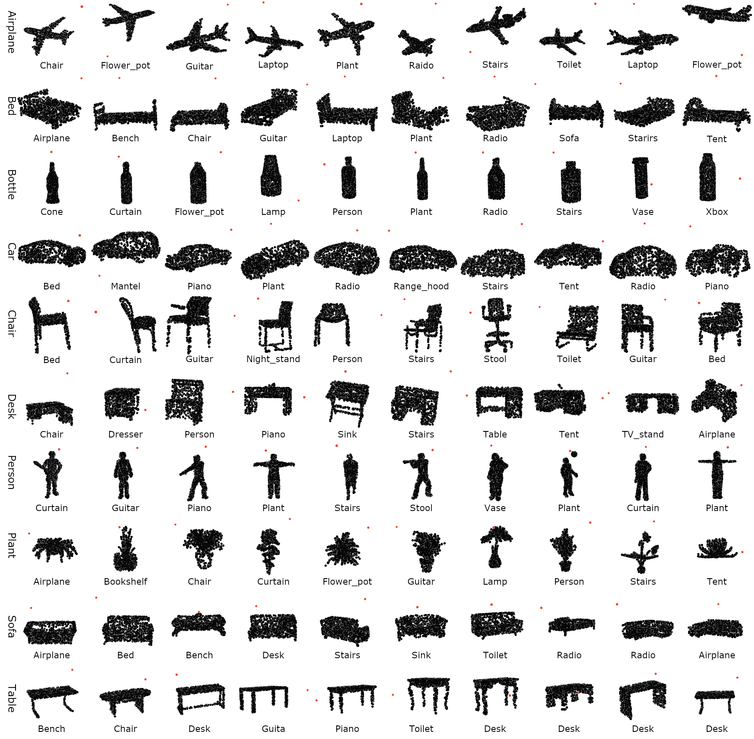
Figure S1: More results from OPA. We chose the $10$ representative classes that appear more frequently in the real world. The perturbed points are indicated in red to be noticeable.

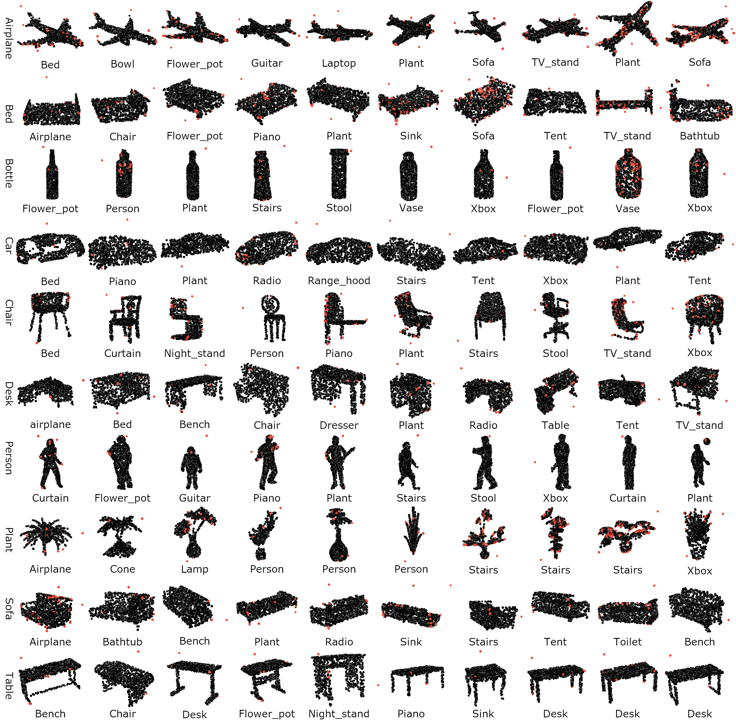
Figure S2: More results from CTA. We also chose the $10$ representative classes that appear more frequently in the real world. The perturbed points are indicated in red to be noticeable.

7.4 Label Diversity of adversarial examples

For non-targeted OPA and CTA, the optimization process diminishes the neurons corresponding to the original labels, with no interest in the predicted labels of the adversarial examples. However, we found that observing the adversarial labels helped to understand the particularities of the adversarial examples. Fig. S3 and S4 report the label distribution matrices of untargeted OPA and CTA respectively. As can be seen from Fig. S3, class ”radio” is most likely to be the adversarial label, and most of the adversarial examples generated within the same class are concentrated in one of the other categories (e.g. almost all instances from ”door” are optimized towards ”curtain”). This phenomenon is significantly ameliorated in CTA (see Fig. S4). The target labels are more evenly distributed in the target label matrix, yielding more diversity in the adversarial examples.

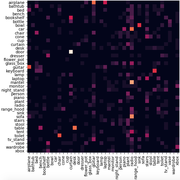
Figure S3: Heat map of successful attacks by OPA across labels. Rows indicate from which category the adversarial examples come and the columns indicate to which category they are predicted. The brighter the square, the more examples that fall into the corresponding category.

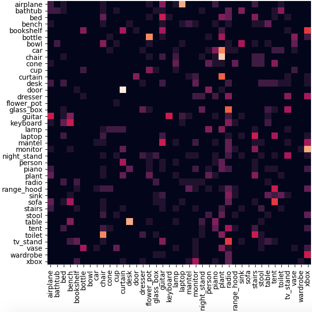
Figure S4: Heat map of successful attacks by CTA across labels. Rows indicate from which category the adversarial examples come and the columns indicate to which category they are predicted. The brighter the square, the more examples that fall into the corresponding category.

7.5 Hyper-parameter settings

7.5.1 Distance regularization $\beta$

For both proposed algorithms, there are two crucial hyper-parameters to be tuned that affect the performance of the attacks, i.e. $\alpha$ and $\beta$. $\alpha$ indicates the optimization rate and is empirically set to $1e-6$. $\beta$ indicates the penalty of perturbation distances, which regularizes the shifting magnitude and preserves the imperceptibility of adversarial examples. In previous experiments, we temporarily set $\beta$ to $0$ to highlight the sparse perturbation dimensions. However, additional investigations suggest that appropriate $beta$ can further improve the performance of the proposed approaches. Fig. S5 demonstrates the performances with different $\beta$ settings. Interestingly, we found that CTA performs best when $\beta=\alpha$: while maintaining nearly $100\%$ success rate and comparably shifting distances, its average $N_{p}$ dramatically decreases to $3.04$ (different from OPA, CTA employs no random-noise). We strongly recommend restricting $\beta$ to a reasonable range ($\leq(8\times\alpha)$) since large $\beta$ easily leads to an explosion in processing time.

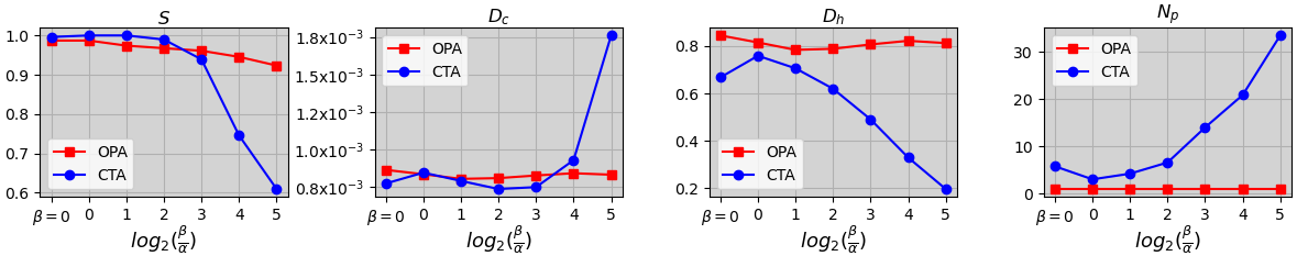
Figure S5: Performance (success rate, Chamfer and Hausdorff distances and the number of shifted points respectively) of OPA and CTA in different settings of hyper-parameters. The x-axis indicates the logarithm of the quotient of $\beta$ and $\alpha$ where the first tick denotes $\beta=0$.

7.5.2 Gaussian noise weight $W_{n}$ for OPA

In particular for OPA, another hyperparameter $W_{n}$ is set to prevent the optimization process from stagnating at a local optimum. We experimented with various settings of $W_{n}$ and present the results in Fig. S6. What stands out in the figure is that the appropriate range for $W_{n}$ is around $10^{-1}$ to $10^{-0.5}$ where the success rate approximates $100\%$ while maintaining acceptable perturbation distances. Adding Gaussian noise in the optimization process dramatically enhances the attack performance of OPA, with its success rate increasing from $56.1\%$ as a simple-gradient attack to almost $100\%$. Interestingly, we observe that a suitable noise weight concurrently reduces the perturbation distance and thus augments the imperceptibility of the adversarial examples. We attribute this to the promotion of Gaussian noise that facilitates the optimizer to escape from saddle planes or local optimums faster, reducing the number of total iterations. However, overweighting deviates the critical point from the original optimization path, which is equivalent to resetting another starting position in 3D space and forcing the optimizer to start iterating again. While there remains a high probability of finding an adversarial example, its imperceptibility is severely impaired.

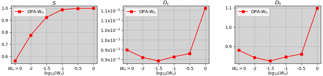
Figure S6: Performance (success rate, Chamfer and Hausdorff distances respectively) of OPA in different settings of weights for Gaussian noise. The x-axis indicates the logarithm of $W_{n}$ where the first tick denotes $W_{n}=0$.

7.6 OPA on 2D image neural network

For a relatively fair comparison as a reference, we extend our OPA to 2D image neural networks for a rough comparison of its sensitivity to critical points with that of 3D networks. We trained a simple ResNet18 network with the MNIST handwriting dataset, which achieves an accuracy of $99\%$ on the test set. We select $1000$ samples from the test set as victims to be attacked with OPA. The quantitative results and parts of the adversarial examples are demonstrated in table S1 and Fig. S7 respectively. In Fig. S7, the original instances and their adversarial results are listed on the first and the second row respectively. With the removal of a pixel in a critical location, a small number of test images successfully fooled the neural network. However, from a quantitative viewpoint (table S1), shifting one critical point almost fails to fool the ResNet18 network ($1.2\%$ success rate for ResNet18-GR). We believe the reasons are: (1) 2D images are restricted within the RGB/greyscale space, thus there exists an upper bound on the magnitude of the perturbation, while 3D point clouds are infinitely extendable; (2) Large-size convolutional kernels ($\geq 2$) learn local features of multiple pixels, which mitigates the impact of individual points on the overall prediction. According to observation (1), we temporarily remove the physical limitation during attacks to investigate the pure mechanism inside both networks and report the results in ResNet18-GF of table S1. Though the attack success rate climbs to $51.7\%$, there is still a gap with PointNet ($98.7\%$). PointNet encodes points with $1\times 1$ convolutional kernels, which is analogous to an independent weighting process for each point. The network inclines to assign a large weight to individual points due to the weak local correlation of adjacent points and therefore leads to vulnerable robustness against perturbations of critical points.

	S	$D_{c}$	$D_{h}$
ResNet18-GR	$1.2$	$4.93\times 10^{-2}$	$8.67\times 10^{-1}$
ResNet18-GF	$51.7$	$1.48$	$4.08\times 10^{1}$
PointNet	$98.7$	$8.64\times 10^{-4}$	$8.45\times 10^{-1}$

Table S1: OPA attack performance comparisons between ResNet18 and PointNet. ResNet18-GR indicates the attack within the range restriction of the greyscale value ($0\sim 255$), while ResNet18-GF indicates a purely numerical attack possibly with no physical significance (greyscale value less than $0$ or greater than $255$).

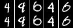
Figure S7: Successful attack examples of ResNet18-GR by OPA. The first and second rows are input images and adversarial examples respectively.

7.7 Additional Activation Maximization (AM) results

For fairness and persuasion, we conduct AM experiments with various initializations as a supplement of section 5.1. Fig. S8 shows AM initialized with zeros and the point cluster generated by averaging all test data [26].

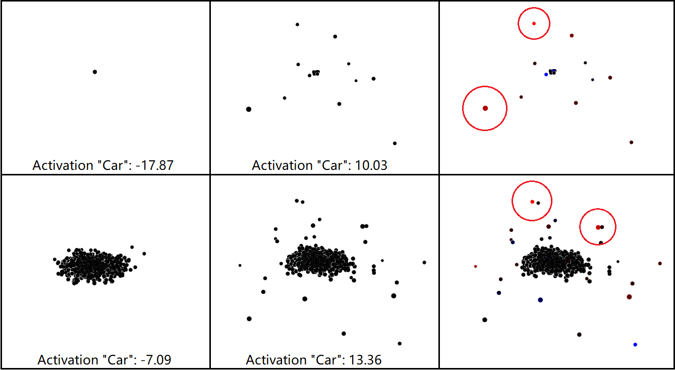
Figure S8: AM results initialized with zeros (the first row) and the point cluster generated by averaging all test data (the second row) respectively. The first, second and third columns demonstrate the initialized set of points, the AM output results after $1000$ optimization steps and the salience map explanation of the corresponding output explained by IG, respectively. In the explanation, red points indicate the degree of positive attributions.

7.8 Visualization of the attribution distributions

As a supplementary of table 6, we demonstrate the complete pie diagrams of the attribution distributions of the aforementioned four pooling structures in S9.

7.9 Societal impacts and ethical issues

This work proposes two adversarial approaches, which pose a potential threat to the security of PC networks. Motivationally, however, this paper aims to illuminate the distribution of attributions of PC networks rather than specifically targeting the attack method of the model. Practically, our proposed approaches can be more easily defended visually or algorithmically compared to related studies aiming at imperceptibility. Table S2 presents the results of defending against the proposed attacks by a simple outlier removal algorithm. Adversarial samples generated by OPA and CTA are detected with almost $100\%$ success rate. We thus argue that the proposed attacks do not pose a serious threat to existing networks.

	$r_{D}$	$r_{P}$
OPA	98.6	100
CTA	99.2	45.6

Table S2: Success rates of defense against the proposed attacks by outlier removal. $r_{D}$ denotes the success rate of the input instance being detected as adversarial examples and $r_{P}$ denotes the percentage of perturbation points detected by the defense module correctly.

References

- [1] Julius Adebayo, Justin Gilmer, Michael Muelly, Ian Goodfellow, Moritz Hardt, and Been Kim. Sanity checks for saliency maps. arXiv preprint arXiv:1810.03292, 2018.
- [2] Naveed Akhtar and Ajmal Mian. Threat of adversarial attacks on deep learning in computer vision: A survey. Ieee Access, 6:14410–14430, 2018.
- [3] George A Alvarez and Patrick Cavanagh. The capacity of visual short-term memory is set both by visual information load and by number of objects. Psychological science, 15(2):106–111, 2004.
- [4] Nadia Burkart and Marco F Huber. A survey on the explainability of supervised machine learning. Journal of Artificial Intelligence Research, 70:245–317, 2021.
- [5] Ruth MJ Byrne. Counterfactuals in explainable artificial intelligence (xai): Evidence from human reasoning. In IJCAI, pages 6276–6282, 2019.
- [6] Nicholas Carlini and David Wagner. Towards evaluating the robustness of neural networks. In 2017 ieee symposium on security and privacy (sp), pages 39–57. IEEE, 2017.
- [7] Angel X Chang, Thomas Funkhouser, Leonidas Guibas, Pat Hanrahan, Qixing Huang, Zimo Li, Silvio Savarese, Manolis Savva, Shuran Song, Hao Su, et al. Shapenet: An information-rich 3d model repository. arXiv preprint arXiv:1512.03012, 2015.
- [8] Susanne Dandl, Christoph Molnar, Martin Binder, and Bernd Bischl. Multi-objective counterfactual explanations. In International Conference on Parallel Problem Solving from Nature, pages 448–469. Springer, 2020.
- [9] Yinpeng Dong, Fangzhou Liao, Tianyu Pang, Hang Su, Jun Zhu, Xiaolin Hu, and Jianguo Li. Boosting adversarial attacks with momentum. In Proceedings of the IEEE conference on computer vision and pattern recognition, pages 9185–9193, 2018.
- [10] Robert Dorfman. A formula for the gini coefficient. The review of economics and statistics, pages 146–149, 1979.
- [11] Dumitru Erhan, Yoshua Bengio, Aaron Courville, and Pascal Vincent. Visualizing higher-layer features of a deep network. University of Montreal, 1341(3):1, 2009.
- [12] Ian J Goodfellow, Jonathon Shlens, and Christian Szegedy. Explaining and harnessing adversarial examples. arXiv preprint arXiv:1412.6572, 2014.
- [13] Yash Goyal, Ziyan Wu, Jan Ernst, Dhruv Batra, Devi Parikh, and Stefan Lee. Counterfactual visual explanations. In International Conference on Machine Learning, pages 2376–2384. PMLR, 2019.
- [14] Ananya Gupta, Simon Watson, and Hujun Yin. 3d point cloud feature explanations using gradient-based methods. In 2020 International Joint Conference on Neural Networks (IJCNN), pages 1–8. IEEE, 2020.
- [15] Abdullah Hamdi, Sara Rojas, Ali Thabet, and Bernard Ghanem. Advpc: Transferable adversarial perturbations on 3d point clouds. In European Conference on Computer Vision, pages 241–257. Springer, 2020.
- [16] Mark T Keane and Barry Smyth. Good counterfactuals and where to find them: A case-based technique for generating counterfactuals for explainable ai (xai). In International Conference on Case-Based Reasoning, pages 163–178. Springer, 2020.
- [17] Jaeyeon Kim, Binh-Son Hua, Thanh Nguyen, and Sai-Kit Yeung. Minimal adversarial examples for deep learning on 3d point clouds. In Proceedings of the IEEE/CVF International Conference on Computer Vision, pages 7797–7806, 2021.
- [18] Diederik P Kingma and Jimmy Ba. Adam: A method for stochastic optimization. arXiv preprint arXiv:1412.6980, 2014.
- [19] Alexey Kurakin, Ian Goodfellow, Samy Bengio, et al. Adversarial examples in the physical world, 2016.
- [20] Kibok Lee, Zhuoyuan Chen, Xinchen Yan, Raquel Urtasun, and Ersin Yumer. Shapeadv: Generating shape-aware adversarial 3d point clouds. arXiv preprint arXiv:2005.11626, 2020.
- [21] Xinke Li, Zhirui Chen, Yue Zhao, Zekun Tong, Yabang Zhao, Andrew Lim, and Joey Tianyi Zhou. Pointba: Towards backdoor attacks in 3d point cloud, 2021.
- [22] Daniel Liu, Ronald Yu, and Hao Su. Extending adversarial attacks and defenses to deep 3d point cloud classifiers. In 2019 IEEE International Conference on Image Processing (ICIP), pages 2279–2283. IEEE, 2019.
- [23] Daniel Liu, Ronald Yu, and Hao Su. Adversarial shape perturbations on 3d point clouds. In European Conference on Computer Vision, pages 88–104. Springer, 2020.
- [24] George A Miller. The magical number seven, plus or minus two: Some limits on our capacity for processing information. Psychological review, 63(2):81, 1956.
- [25] Seyed-Mohsen Moosavi-Dezfooli, Alhussein Fawzi, and Pascal Frossard. Deepfool: a simple and accurate method to fool deep neural networks. In Proceedings of the IEEE conference on computer vision and pattern recognition, pages 2574–2582, 2016.
- [26] Anh Nguyen, Jason Yosinski, and Jeff Clune. Multifaceted feature visualization: Uncovering the different types of features learned by each neuron in deep neural networks. arXiv preprint arXiv:1602.03616, 2016.
- [27] Anh Nguyen, Jason Yosinski, and Jeff Clune. Understanding neural networks via feature visualization: A survey. In Explainable AI: interpreting, explaining and visualizing deep learning, pages 55–76. Springer, 2019.
- [28] Nicolas Papernot, Patrick McDaniel, Ian Goodfellow, Somesh Jha, Z Berkay Celik, and Ananthram Swami. Practical black-box attacks against machine learning. In Proceedings of the 2017 ACM on Asia conference on computer and communications security, pages 506–519, 2017.
- [29] Charles R Qi, Hao Su, Kaichun Mo, and Leonidas J Guibas. Pointnet: Deep learning on point sets for 3d classification and segmentation. In Proceedings of the IEEE conference on computer vision and pattern recognition, pages 652–660, 2017.
- [30] Charles R Qi, Li Yi, Hao Su, and Leonidas J Guibas. Pointnet++: Deep hierarchical feature learning on point sets in a metric space. arXiv preprint arXiv:1706.02413, 2017.
- [31] Karen Simonyan, Andrea Vedaldi, and Andrew Zisserman. Deep inside convolutional networks: Visualising image classification models and saliency maps, 2014. arXiv preprint, arXiv:1312.6034.
- [32] Jost Tobias Springenberg, Alexey Dosovitskiy, Thomas Brox, and Martin Riedmiller. Striving for simplicity: The all convolutional net, 2015. arXiv preprint, arXiv:1412.6806.
- [33] Jiawei Su, Danilo Vasconcellos Vargas, and Kouichi Sakurai. One pixel attack for fooling deep neural networks. IEEE Transactions on Evolutionary Computation, 23(5):828–841, 2019.
- [34] Jiachen Sun, Karl Koenig, Yulong Cao, Qi Alfred Chen, and Z Morley Mao. On the adversarial robustness of 3d point cloud classification. arXiv preprint arXiv:2011.11922, 2020.
- [35] Mukund Sundararajan, Ankur Taly, and Qiqi Yan. Gradients of counterfactuals. arXiv preprint arXiv:1611.02639, 2016.
- [36] Mukund Sundararajan, Ankur Taly, and Qiqi Yan. Axiomatic attribution for deep networks. In International Conference on Machine Learning, pages 3319–3328. PMLR, 2017.
- [37] Christian Szegedy, Wojciech Zaremba, Ilya Sutskever, Joan Bruna, Dumitru Erhan, Ian Goodfellow, and Rob Fergus. Intriguing properties of neural networks. arXiv preprint arXiv:1312.6199, 2013.
- [38] Hanxiao Tan and Helena Kotthaus. Surrogate model-based explainability methods for point cloud nns. In Proceedings of the IEEE/CVF Winter Conference on Applications of Computer Vision, pages 2239–2248, 2022.
- [39] Tom Vermeire and David Martens. Explainable image classification with evidence counterfactual. arXiv preprint arXiv:2004.07511, 2020.
- [40] Yue Wang, Yongbin Sun, Ziwei Liu, Sanjay E Sarma, Michael M Bronstein, and Justin M Solomon. Dynamic graph cnn for learning on point clouds. Acm Transactions On Graphics (tog), 38(5):1–12, 2019.
- [41] Yuxin Wen, Jiehong Lin, Ke Chen, C. L. Philip Chen, and Kui Jia. Geometry-aware generation of adversarial point clouds, 2020.
- [42] Matthew Wicker and Marta Kwiatkowska. Robustness of 3d deep learning in an adversarial setting. In Proceedings of the IEEE/CVF Conference on Computer Vision and Pattern Recognition, pages 11767–11775, 2019.
- [43] Zhirong Wu, Shuran Song, Aditya Khosla, Fisher Yu, Linguang Zhang, Xiaoou Tang, and Jianxiong Xiao. 3d shapenets: A deep representation for volumetric shapes. In Proceedings of the IEEE conference on computer vision and pattern recognition, pages 1912–1920, 2015.
- [44] Chong Xiang, Charles R Qi, and Bo Li. Generating 3d adversarial point clouds. In Proceedings of the IEEE/CVF Conference on Computer Vision and Pattern Recognition, pages 9136–9144, 2019.
- [45] Jinlai Zhang, Lyujie Chen, Binbin Liu, Bo Ouyang, Qizhi Xie, Jihong Zhu, and Yanmei Meng. 3d adversarial attacks beyond point cloud. arXiv preprint arXiv:2104.12146, 2021.
- [46] Qiang Zhang, Jiancheng Yang, Rongyao Fang, Bingbing Ni, Jinxian Liu, and Qi Tian. Adversarial attack and defense on point sets. arXiv preprint arXiv:1902.10899, 2019.
- [47] Yue Zhao, Yuwei Wu, Caihua Chen, and Andrew Lim. On isometry robustness of deep 3d point cloud models under adversarial attacks. In Proceedings of the IEEE/CVF Conference on Computer Vision and Pattern Recognition, pages 1201–1210, 2020.
- [48] Tianhang Zheng, Changyou Chen, Junsong Yuan, Bo Li, and Kui Ren. Pointcloud saliency maps. In Proceedings of the IEEE/CVF International Conference on Computer Vision, pages 1598–1606, 2019.
- [49] Hang Zhou, Dongdong Chen, Jing Liao, Kejiang Chen, Xiaoyi Dong, Kunlin Liu, Weiming Zhang, Gang Hua, and Nenghai Yu. Lg-gan: Label guided adversarial network for flexible targeted attack of point cloud based deep networks. In Proceedings of the IEEE/CVF Conference on Computer Vision and Pattern Recognition, pages 10356–10365, 2020.
- [50] Hang Zhou, Kejiang Chen, Weiming Zhang, Han Fang, Wenbo Zhou, and Nenghai Yu. Dup-net: Denoiser and upsampler network for 3d adversarial point clouds defense. In Proceedings of the IEEE/CVF International Conference on Computer Vision, pages 1961–1970, 2019.