Velocity Level Approximation of Pressure Field Contact Patches

Abstract

Pressure Field Contact (PFC) was recently introduced as a method for detailed modeling of contact interface regions at rates much faster than elasticity-theory models, while at the same time predicting essential trends and capturing rich contact behavior. The PFC model was designed to work in conjunction with error-controlled integration at the acceleration level. Therefore a vast majority of existent multibody codes using solvers at the velocity level cannot incorporate PFC in its original form. In this work we introduce a discrete in time approximation of PFC making it suitable for use with existent velocity-level time steppers and enabling execution at real-time rates. We evaluate the accuracy and performance gains of our approach and demonstrate its effectiveness in simulating relevant manipulation tasks. The method is available in open source as part of Drake’s Hydroelastic Contact model.

I Introduction

There is a need for smooth, rich, artifact-free models of contact between arbitrary geometries as encountered in modern robotics applications such as grasping and manipulation, assistive and rehabilitative robotics, prosthetics, and unstructured environments. Most often these applications involve compliant surfaces such as padded grippers, deformable manipuland objects or soft surfaces for safe human-robot interaction. Moreover, with the emerging field of soft robotics, designers have begun to incorporate significant compliance in their robot designs; consider for instance the Soft-bubble gripper [1] in Fig. 1 for which the accurate prediction of contact patches is critical for meaningful sim-to-real transfer. Still, the rigid-body approximation of contact is at the core of many simulation engines enabling them to run at interactive rates.

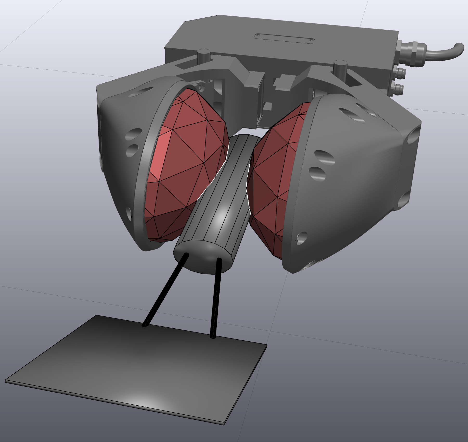
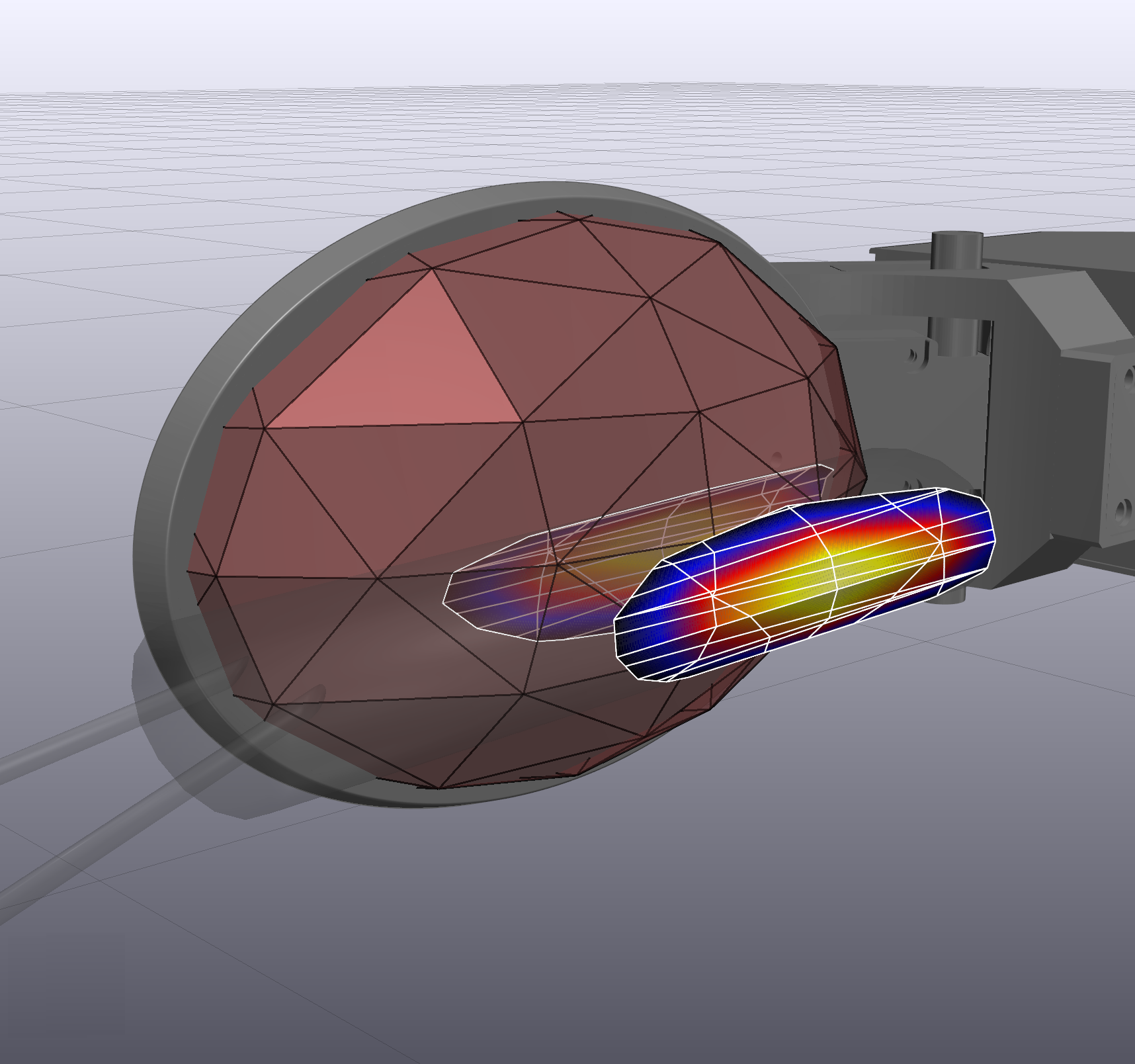
Figure 1: Left: Contact geometry modeling the highly compliant Soft-bubble gripper [1] holding a spatula. Right: One of the fingers is hidden to better show the simulated contact patch. With a coarse discretization, the model is able to predict patch shape, size, and contact pressure (shown as colored contours) along with net forces and moments. Our polygonal tessellation of the contact surface combined with our velocity-level time stepping approximation enables this simulation to run at real-time rates.

Point contact is a useful and popular approximation of non-conforming contact (e.g. contact between a sphere and a half-space), but it does not extend well to conforming surfaces nor non-convex shapes. Localized compliance can be incorporated using spring-dampers [2], Hertz theory [3] and volumetric models [4, 5]. However, while point contact modeling approaches are fast, they are non-smooth, and extensions to arbitrary geometry often involve non-physical heuristics [6, 7] that heavily influence the correctness and accuracy of simulation results [8].

The Elastic Foundation Model [9] (EFM) computes rich contact patches providing an alternative to point contact that can solve many of its issues. However, current implementations [10] need highly refined meshes and can even miss contact interactions if coarse meshes are used. The work in [11] introduces pressure field contact; a modern rendition of EFM designed to work with coarse meshes at a computational cost suitable for real-time simulation. While previous work focuses on smooth geometric queries and continuous penalty forces, see for instance [12, 13, 14], the work in [11] is different in that it introduces a new contact model rather than algorithms for an already existing model. An implementation of pressure field contact is available in open source as part of Drake’s [15] Hydroelastic Contact model. The implementation in Drake includes support for primitive geometries such as spheres and boxes, convex meshes, rigid objects and both triangular and polygonal tessellations, see Section III for details. The hydroelastic contact model provides rich information such as contact patch shape and pressure distribution, see Fig. 1 for an example.

The hydroelastic contact model is originally formulated at the acceleration level in [11] resulting in a system of ODEs advanced forward in time using error-controlled integration. While error-controlled integration guarantees the accuracy of the solutions, it comes with the additional cost of needing to compute error estimates and taking smaller time steps during stick/slip transitions.

In contrast, popular simulation engines such as ODE [16], Dart [17], Vortex [18], MuJoCo [19] and Drake [15] provide formulations at the velocity-level. In this approach, time is advanced at discrete intervals of fixed size; contact impulses and the resulting velocities are found by solving a challenging Nonlinear Complementarity Problem (NCP), or some approximation of an NCP.

Our main contribution with this work is a discrete in time approximation of the hydroelastic contact model that enables its use within existent simulation engines formulated at the velocity-level. We derive an algebraic expression for the rate of change of the pressure field in terms of local quantities and use it to write an implicit in time approximation of the pressure field at the centroids of mesh elements. Finally, we cast the problem in terms of an equivalent set of compliant point contact forces that can be incorporated into existent velocity-level formulations.

This work also introduces a novel polygonal representation of the contact surfaces introduced in [11]. We strive to enable simulation of contact rich patches, eliminate artifacts introduced by point contact, and capture area dependent phenomena otherwise missed by point contact while still performing at real-time rates. This is achieved with a complete implementation in Drake [15].

II Multibody Dynamics With Frictional Contact

Here we closely follow the notation in our previous work [20, 21] for consistency. However, we point out that velocity-level engines with the capability to model compliant point contact can incorporate the approximations introduced in this work to model compliant contact patches using the hydroelastic contact model. For stability, our approximations are implicit in time.

The state of our system is described by the generalized positions ${\mathbf{q}}\in\mathbb{R}^{n_{q}}$ and the generalized velocities ${\mathbf{v}}\in\mathbb{R}^{n_{v}}$, where $n_{q}$ and $n_{v}$ denote the number of generalized positions and velocities, respectively. Time derivatives of the configurations are related to the generalized velocities by $\dot{{\mathbf{q}}}={\mathbf{N}}({\mathbf{q}}){\mathbf{v}}$, with ${\mathbf{N}}({\mathbf{q}})\in\mathbb{R}^{n_{q}\times n_{v}}$ the kinematic map.

II-A Contact Kinematics

Given a configuration ${\mathbf{q}}$ of the system, we assume our geometry engine reports a set $\mathscr{C}({\mathbf{q}})$ of $n_{c}$ potential contacts between pairs of bodies. The $i\text{-th}$ contact pair in $\mathscr{C}({\mathbf{q}})$ is characterized by its location, a contact normal $\hat{{\bm{n}}}_{i}$, and the signed distance $\phi_{i}\in\mathbb{R}$, defined negative for overlapping bodies. The relative velocity between the pair of bodies at the contact point is denoted with ${\bm{v}}_{c,i}\in\mathbb{R}^{3}$. The normal and tangential components of ${\bm{v}}_{c,i}$ are given by $v_{n,i}=\hat{{\bm{n}}}_{i}\cdot{\bm{v}}_{c,i}$ and ${\bm{v}}_{t,i}={\bm{v}}_{c,i}-v_{n,i}\hat{{\bm{n}}}_{i}$ respectively, so that ${\bm{v}}_{c,i}=[{\bm{v}}_{t,i}\,v_{n,i}]$. We form vector ${\mathbf{v}}_{c}\in\mathbb{R}^{3n_{c}}$ (bold, no italics) by stacking the velocities ${\bm{v}}_{c,i}$. Contact velocities are related to generalized velocities by ${\mathbf{v}}_{c}={\mathbf{J}}({\mathbf{q}}){\mathbf{v}}$, where ${\mathbf{J}}$ is the contact Jacobian.

II-B Contact Modeling

A popular point contact model of compliance introduces a spring/damper at each contact point to model the normal force $f_{n}$ as

$$f_{n}=(-k\phi-d\,v_{n})_{+},$$ (1)

where $k>0$ is the point contact stiffness and $d>0$ is a coefficient of linear dissipation, and $x_{+}=\max(x,0)$ is the positive part operator. Since we take the positive part, the force is always repulsive. This model can be cast as the equivalent complementarity condition [22]

$$0\leq\phi+d\,c\,v_{n}+c\,f_{n}\perp f_{n}\geq 0,$$ (2)

where $c=k^{-1}$ is the compliance and $0\leq a\perp b\geq 0$ denotes complementarity, i.e. $a\geq 0$, $b\geq 0$ and $a\,b=0$. Using the first order approximation $\phi=\phi_{0}+\delta t\,v_{n}$ where $\phi_{0}$ is the signed distance function at the previous time step and $\delta t$ is step size, Eq. (2) becomes a linear complementarity condition between the velocities of the system and the contact forces. We use the naught subscript to denote quantities evaluated at the previous time step while no subscript is used for quantities evaluated at the next time step.

$$0\leq\phi_{0}+(\delta t+d\,c)v_{n}+c\,f_{n}\perp f_{n}\geq 0.$$ (3)

The tangential component ${\bm{f}}_{t}\in\mathbb{R}^{2}$ of the contact forces is modeled according to Coulomb’s law of dry friction, which can be compactly written as

$${\bm{f}}_{t}=\operatorname*{arg\,min}_{\|{\bm{f}}\|\leq\mu f_{n}}{\bm{v}}_{t}\cdot{\bm{f}}$$ (4)

where $\mu>0$ is the coefficient of friction. Equation (4) describes the maximum dissipation principle, which states that friction forces maximize the rate of energy dissipation. In other words, friction forces oppose the sliding velocity direction. Moreover, Eq. (4) states that contact forces ${\bm{f}}_{c}$ are constrained to belong to the friction cone $\mathcal{F}=\{[{\bm{x}}_{t},x_{n}]\in\mathbb{R}^{3}\,|\,\|{\bm{x}}_{t}\|\leq\mu x_{n}\}$.

The optimality conditions for Eq. (4) are [23, 24]

$$\mu f_{n}{\bm{v}}_{t}+\lambda{\bm{f}}_{t}={\bm{0}}$$

$$0\leq\lambda\perp\mu f_{n}-\|{\bm{f}}_{t}\|\geq 0$$ (5)

where $\lambda$ is the multiplier needed to enforce Coulomb’s law condition $\|{\bm{f}}_{t}\|\leq\mu f_{n}$. Notice that in the form we wrote Eq. (5), multiplier $\lambda$ has units of velocity and it is zero during stiction and takes the value $\lambda=\|{\bm{v}}_{t}\|$ during sliding. Finally, the total contact force ${\bm{f}}_{c}\in\mathbb{R}^{3}$ expressed in the contact frame $C$ is given by ${\bm{f}}_{c}=[{\bm{f}}_{t}\,f_{n}]$.

II-C Discrete Time Stepping

We discretize time into intervals of fixed size $\delta t$ and seek to advance the state of the system from time $t^{n}$ to the next step at $t^{n+1}=t^{n}+\delta t$. To simplify notation, we use the naught subscript to denote quantities evaluated at the previous time step $t^{n}$ while no additional subscript is used for quantities at the next time step $t^{n+1}$. The full contact problem consists of the balance of momentum discretized in time together with the full set of contact constraints, where the unknowns are the next time step generalized velocities ${\mathbf{v}}\in\mathbb{R}^{n_{v}}$, forces ${\mathbf{f}}\in\mathbb{R}^{3n_{c}}$ and multipliers ${\bm{\lambda}}\in\mathbb{R}^{n_{c}}$

$${\mathbf{M}}_{0}({\mathbf{v}}-{\mathbf{v}}_{0})=\delta t\,{\mathbf{k}}_{0}+\delta t\,{\mathbf{J}}_{0}^{T}{\mathbf{{\mathbf{f}}}},$$ (6)

$$0\leq\phi_{0,i}+(\delta t+d_{i}\,c_{i})\,v_{n,i}+c_{i}f_{n,i}$$

$$\qquad\perp f_{n,i}\geq 0,\quad\qquad\qquad\qquad\!i\in\mathscr{C}({\mathbf{q}}_{0})$$ (7)

$$\mu_{i}f_{n,i}{\bm{v}}_{t,i}+\lambda_{i}{\mathbf{f}}_{t,i}={\bm{0}},\qquad\qquad\,\,i\in\mathscr{C}({\mathbf{q}}_{0})$$ (8)

$$0\leq\lambda_{i}\perp\mu_{i}f_{n,i}-\|{\mathbf{f}}_{t,i}\|\geq 0,\!\!\qquad i\in\mathscr{C}({\mathbf{q}}_{0})$$ (9)

$${\mathbf{q}}={\mathbf{q}}_{0}+\delta t{\mathbf{N}}_{0}{\mathbf{v}},$$ (10)

where ${\mathbf{M}}_{0}\in\mathbb{R}^{n_{v}\times n_{v}}$ is the mass matrix and ${\mathbf{k}}_{0}\in\mathbb{R}^{n_{v}}$ models external forces such as gravity, gyroscopic terms and other smooth generalized forces such as those arising from springs and dampers.

We note that typically these velocity-level formulations are written in terms of impulses $\delta t{\mathbf{{\mathbf{f}}}}$. The full problem (6)-(10) constitutes a nonlinear complementarity problem (NCP). Many variants of this formulation exist in the literature. [25] introduces both primal and dual formulations of the problem, [26] uses barrier functions along a lagged dissipative potential to include friction, [23] uses a polyhedral approximation of the friction cone to write a linear complementarity problem (LCP).

In the next section we describe an approximation that allows one to incorporate the hydroelastic contact model into velocity-level NCP formulations of this type. The approach is general in that it can be incorporated into any velocity-level solver that supports the modeling of compliant point contact.

III Overview of the Hydroelastic Contact Model

The hydroelastic contact model [11] combines two ideas: elastic foundation and hydrostatic pressure. Thus the model introduces an object-centric virtual or elastic pressure field $p_{e}$ to mimic the hydrostatic pressure field of a fluid. In practice, Drake generates a pressure field for primitive shapes that is maximum at the medial axis, zero at the boundary, and linearly interpolated in between. In Drake, users specify how stiff a compliant object is through the hydroelastic modulus $E_{h}$ [27], the value of the pressure field at the medial axis. How to generate pressure fields for arbitrary non-convex geometries is currently a topic of active research.

Unlike Finite Element models, the hydroelastic contact model is stateless and the deformed configuration of a body is approximated. Given two overlapping (undeformed) objects $A$ and $B$ with pressure fields $p_{A}$ and $p_{B}$, respectively, the contact surface $\mathcal{S}^{\cap}$ is modeled as the surface of equal pressure, see Fig. 2. Total forces and moments on these bodies are the result of the integral of the equilibrium pressure field $p_{e}=p_{A}=p_{B}$ on the contact surface $\mathcal{S}^{\cap}$.

Figure 2: Two overlapping compliant bodies with pressure fields $p_{A}$ and $p_{B}$, with profiles along the normal direction sketched in dashed lines. The contact surface $\mathcal{S}^{\cap}$ is modeled as the surface of equal pressure. We consider the motion of the surface along the normal direction $\hat{{\bm{n}}}$, taking into account directional gradients $g_{A}=-dp_{A}/dn=-\nabla p_{A}\cdot\hat{{\bm{n}}}$ and $g_{B}=dp_{B}/dn=\nabla p_{B}\cdot\hat{{\bm{n}}}$.

III-A Contact Surface Computation

We represent the geometry of a compliant body with a tetrahedral volume mesh. Each vertex of this mesh stores a single scalar pressure value resulting in a piece-wise linear pressure field $p_{e}$ which can be used to interpolate pressure values at any point inside the volume.

The contact surface between two compliant bodies $A$ and $B$ consists of a number of polygons. We denote with $L_{a}:\mathbb{R}^{3}\rightarrow\mathbb{R}$ and $L_{b}:\mathbb{R}^{3}\rightarrow\mathbb{R}$ the linear interpolation of the respective pressure fields within two tetrahedra $\tau_{a}\in A$ and $\tau_{b}\in B$ having a non-empty intersection. Intersecting tetrahedra can be found efficiently with a judicious choice of data structures [11]. The surface on which $L_{a}$ equals $L_{b}$ defines an equilibrium plane $P_{ab}$. The contact surface is the intersection $P_{ab}\cap\tau_{a}\cap\tau_{b}$, a convex polygon with at most eight vertices, Fig. 3. Recall that undeformed bodies are allowed to overlap, see Fig. 2. Therefore intersecting tetrahedra from two bodies as depicted in Fig. 3 is commonplace within the overlap region of Fig. 2.

Figure 3: Steps to compute a contact polygon for compliant-compliant contact. a) Two overlapping tetrahedra. b) Their equilibrium plane is clipped by the bottom tetrahedron into a square. c) The top tetrahedron clips the plane further into the final polygon, in this example, an octagon. d) Contact polygon with linearly interpolated equilibrium pressure.

While a rigid object can be approximated as a compliant hydroelastic object with a very large modulus of elasticity, this approach can lead to numerical issues. Therefore, in Drake, we represent a rigid object solely with a surface mesh of triangles that tessellates its boundary. In this case, the contact surface corresponds to the surface of the rigid object clipped by the volume of the compliant object and the contact pressure $p_{e}$ is the linear interpolation of the compliant pressure field onto the contact surface.

III-B Triangulated vs. Polygonal Contact Surfaces

In [11] an $n$ sided polygon is divided into a fan of $n$ triangles that share a vertex at the polygon’s centroid, left in Fig. 4. This ensures that only zero area triangles are added/removed to the contact surface as objects move so that topological changes do not introduce discontinuities in the contact forces, as required for error-controlled integration.

As we’ll see in Section IV, each face in the contact surface corresponds to one contact constraint in Eq. 7. Therefore to arrive to a smaller contact problem, we seek to minimize the number of contact constraints and consequently the number of discrete faces. We then propose to replace the fan of triangles by the original polygon, right in Fig. 4.

The polygonal representation leads to a significant reduction in the number of face elements representing the surface, a factor of seven in Fig. 4. Even though much coarser, the polygonal representation still provides rich contact information and allows to capture complex area-dependent phenomena. This is demonstrated with test cases of practical relevance in Section V. Finally, the equilibrium pressure field is linear since it results from the intersection of the linear pressure fields of overlapping tetrahedra.

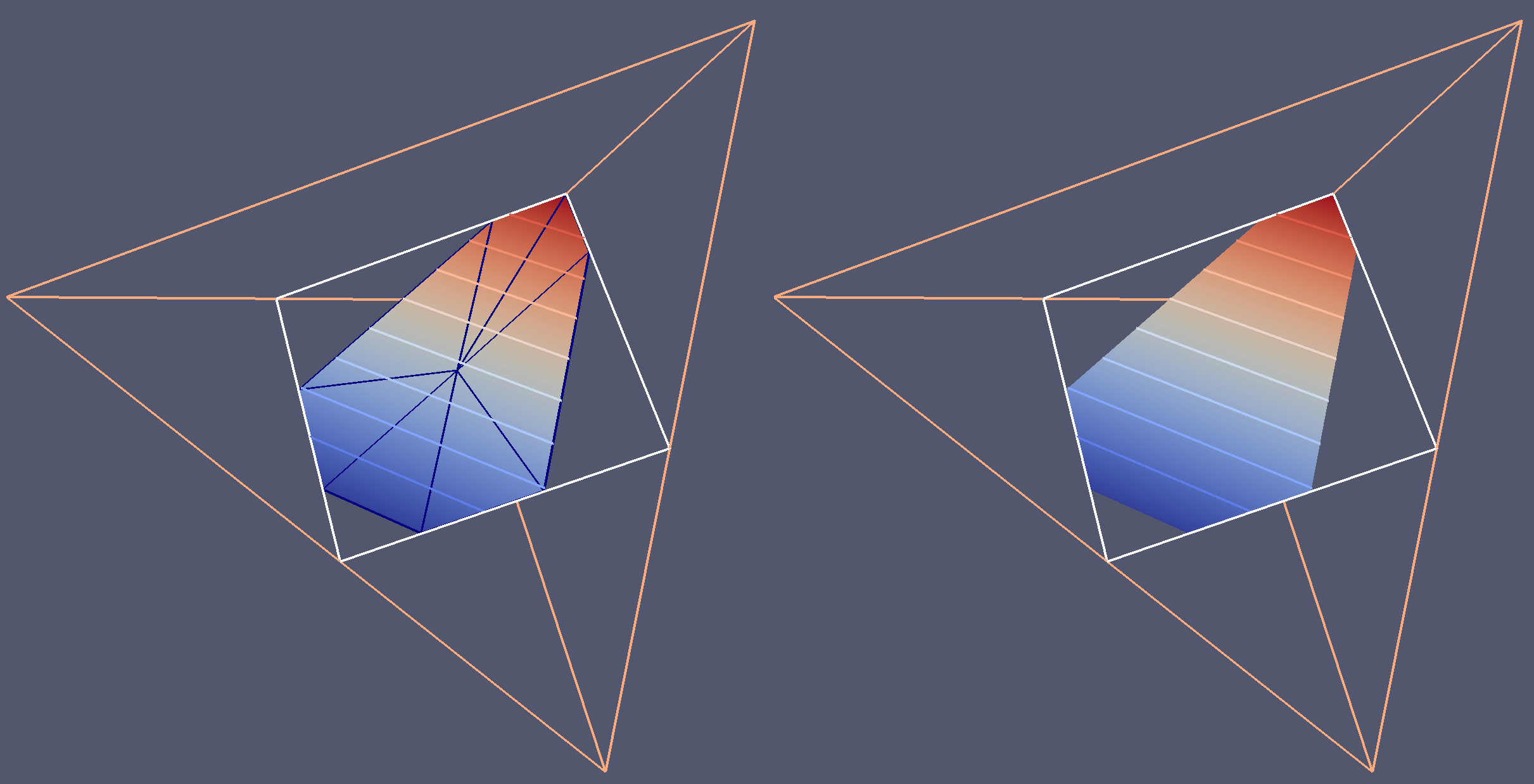
Figure 4: Triangular tessellation (left) as required in [11] and the proposed polygonal approximation (right). The pressure field is linear on the polygon as shown by the contour lines and the color shading. The white rectangle outline is a visual cue for the spanning plane of the contact polygon relative to the compliant tetrahedron drawn in orange outline.

IV Point Contact Approximation

The key idea introduced in this work is to approximate the force contribution from each of the polygons described in Section III-B using a first order expansion in time that resembles the point contact model in Eq. (7). The elastic force contribution ${\bm{f}}_{e}$ from a polygon with area $A$ is the integral of the pressure field

$${\bm{f}}_{e}=\int_{A}p_{e}({\bm{x}})\,\hat{{\bm{n}}}\,dA=\hat{{\bm{n}}}\int_{A}p_{e}({\bm{x}})\,dA$$ (11)

where the second equality results from the fact that faces are planar. Moreover, since the pressure field is linear (Fig. 4), this integral can be computed exactly as

$${\bm{f}}_{e} = f_{n,e}\,\hat{{\bm{n}}},$$

$$f_{n,e} = A\,p_{c}$$ (12)

where $p_{c}=p_{e}({\bm{x}}_{c})$ is the pressure evaluated at the centroid ${\bm{x}}_{c}$ of the polygonal face.

To obtain an approximation consistent with the discrete framework (6)-(10), we use a first order Taylor expansion to approximate the pressure as

$$p_{c}=\left(p_{c,0}+\delta t\,\frac{dp_{c}}{dt}\right)_{+},$$ (13)

where $p_{c,0}$ is the hydroelastic pressure at the previous time step. Since pressure is zero at the boundary of each object and zero outside, we must take the positive part in (13) to properly represent this functional form when bodies break contact.

We will show next that the time rate of the pressure at the surface can be approximated as

$$\frac{dp_{c}}{dt}=-g\,v_{n},$$ (14)

where $g$ is an effective pressure gradient, with units of $\text{Pa}/\text{m}$ and $v_{n}$ is the normal relative velocity at the centroid. Using this approximation in Eqs. (12) and (13), we can write

$$f_{n,e}=(-k\phi)_{+},$$ (15)

with

$$k = g\,A_{0},$$

$$\phi_{0} = -\frac{p_{c,0}}{g},$$

$$\phi = \phi_{0}+\delta t\,v_{n}.$$ (16)

where we froze geometric quantities at the previous time step. This is common practice in many discrete time stepping strategies in the literature, see for instance [28, 29]. Dissipation in (15) is incorporated as in (1) to obtain an equivalent point contact model.

Using this surrogate signed distance $\phi_{0}$ and stiffness $k$ we introduce the contribution of the $i\text{-th}$ face of the contact surface as a compliant point contact constraint in (7). Note that the resulting scheme is implicit in the next time step velocities through (7), making the scheme robust to the choice of time-step size even for stiff materials.

Since these quantities are a function of polygon area and effective pressure gradient, the approximation converges to the original continuous model in the limit to zero time step. Notice this would not be true for a simple model where spring-dampers are located at the polygons’ centroids.

IV-A Pressure Time Rate

At a given point on the contact surface in Fig. 2 we analyze the relative motion of bodies $A$ and $B$ in the direction normal to the surface. We define a coordinate $x$ in the normal direction such that $x=0$ at the surface and it increases in the direction along the normal.

Along this normal direction, in the neighborhood to the contact point, we approximate pressure fields $p_{A}(x)$ and $p_{B}(x)$ as linear functions of the coordinate $x$

$$p_{A}(x) =-g_{A}(x-x_{A}(t))+b_{A},$$ (17)

$$p_{B}(x) =g_{B}(x-x_{B}(t))+b_{B},$$ (18)

where $g_{A}=-\nabla p_{A}\cdot\hat{{\bm{n}}}$ and $g_{B}=\nabla p_{B}\cdot\hat{{\bm{n}}}$ are the slopes along the normal, $x_{A}(t)$ and $x_{B}(t)$ are points rigidly affixed to $A$ and $B$, respectively, and $b_{A}$ and $b_{B}$ are simply the pressure values at $x_{A}(t)$ and $x_{B}(t)$, respectively. This is a reasonable approximation given that the pressure fields are piecewise linear functions within each compliant volume.

The equilibrium pressure at the surface, $x=0$, is found by equating the hydroelastic pressures

$$p_{e}=g_{A}\,x_{A}(t)+b_{A}=-g_{B}\,x_{B}(t)+b_{B}.$$ (19)

We take the time derivative of (19) to find the rate of change of the pressure, as we need it in (13) at each polygon centroid

$$\frac{dp_{e}}{dt}=g_{A}\,v_{A}(t)=-g_{B}\,v_{B}(t),$$ (20)

where $v_{A}(t)$ and $v_{B}(t)$ are the respective velocities of each body along the normal. These velocities are relative to the contact surface since coordinate $x$ is defined relative to the surface, located at all times at $x=0$. Since the pressure fields are fixed in the body frames, $\dot{b}_{A}=\dot{b}_{B}=0$. In terms of these velocities, the normal velocity $v_{n}$ is given by

$$v_{n}=v_{B}-v_{A}$$ (21)

Combining Eqs. (20) and (21) we can write velocities $v_{A}(t)$ and $v_{B}(t)$ in terms of the normal velocity $v_{n}$ as

$$v_{A} = -\frac{g_{B}}{g_{A}+g_{B}}\,v_{n},$$

$$v_{B} = \frac{g_{A}}{g_{A}+g_{B}}\,v_{n}.$$ (22)

The final expression for the rate of change of the pressure at the interface is obtained using the relative velocities from (22) into (20). After some minimal algebraic manipulation, the result is

$$\frac{dp_{e}}{dt}=\frac{-g_{A}\,g_{B}}{g_{A}+g_{B}}v_{n}.$$ (23)

Typically the pressure gradients and the normal direction align along the same line and therefore both $g_{A}$ and $g_{B}$ are positive. In this case $dp/dt<0$ for $v_{n}>0$ and the pressure decreases as the bodies move away from each other, as expected. However, special care must be taken when $g_{A}<0$ or $g_{B}<0$. Since the discrete approximation of point contact requires $k>0$, we simply ignore polygons where the conditions $g_{A}>0$ and $g_{B}>0$ are not satisfied. We find that this is not a major problem in practice since this situation corresponds to corner cases of the hydroelastic contact model for which pushing into the object leads to a decrease of the contact forces instead of an increase as expected.

V Results and Discussion

We present a series of simulation cases to assess the robustness, accuracy, and performance of our method. The time step for each simulation is chosen such that it can properly resolve the dynamics of each specific problem. It is a trade off between accuracy and speed.

In Drake we have two velocity level solvers; TAMSI [20] and SAP [21]. SAP uses a convex approximation of contact excellent for problems dominated by stiction or sliding at low velocities. We use SAP in Section V-B for our scalability studies since it uses supernodal sparse algebra and TAMSI everywhere else.

V-A Sliding and Spinning Disk

To assess the accuracy of our method’s ability to capture the highly non-linear coupling between net force and torque, we study a sliding and spinning disk with a known analytical solution [30].

Based on the dimensions of a U.S. quarter dollar coin, we simulate a disk of radius $R=1.213\text{ cm}$, thickness $t=1.75\text{ mm}$, mass $m=5.67\text{ g}$, friction coefficient $\mu=0.2$, and hydroelastic modulus $E_{h}=1.0\text{ GPa}$ lying flat on a horizontal plane set into motion with initial values of translational velocity $v$ and angular velocity $\omega$. The analytical result for this example establishes a dimensionless parameter $\varepsilon=\frac{v}{\omega R}$ that, regardless of initial conditions, converges to $\varepsilon^{*}\approx 0.653$ as the coin comes to rest. We set initial angular and translational velocities to span initial values $\varepsilon_{0}$ in the range $[0.1;10]$.

A fan of 152 triangles discretizes the circular geometry of the coin. To estimate the error introduced by the discrete geometry, we first simulate our model using error controlled integration to a tight accuracy of $10^{-2}\%$. We find the numerical solution with discrete geometry converges to $\varepsilon_{\text{disc}}^{*}=0.64426$, at only $1.3\%$ error from $\varepsilon^{*}$.

We now use our velocity-level discrete solver with a fixed time step of $\delta t=10^{-3}\text{ s}$ to compute numerical approximations $\varepsilon_{\text{num}}^{*}$ from various initial conditions. Theory [30] predicts a constant $\varepsilon^{*}$ regardless of the initial conditions. The numerical results confirm this prediction within $0.01\text{-}0.5\%$ of $\varepsilon_{\text{disc}}^{*}$ and within $1.3\%$ of $\varepsilon^{*}$, see Fig. 5. Variations in these results are caused by numerical sensitivity to the zero-over-zero limit in $\varepsilon=v/(\omega R)$ as the disk comes to rest.

Finally, we perform a convergence study to verify the convergence of our method. For the reference solutions used in Fig. 6 we use a time step size and grid size an order of magnitude smaller than the smallest size shown in the figures. For each timestep $\delta t$ we define the relative error of the computed trajectory $x_{\delta t}(t)$ vs the reference trajector $x(t)$ as:

$$\varepsilon_{\delta t}=||x(t)_{\delta t}-x(t)||_{2}\big{/}||x(t)||_{2}$$

and likewise for $\varepsilon_{\delta x}$. Our solver TAMSI [20] is first order accurate in time, which is verified with the time step convergence study in Fig. 6. Even though we show that a single point at the centroid of each polygon integrates pressure exactly, Fig. 6 shows a quadratic convergence with grid size. This is due to the fact that moments are proportional to both pressure and position, and therefore are not integrated exactly but with a truncation error quadratic on the grid size. If case this is not clear, the integration of moments is being accounted for by the term ${\mathbf{J}}_{0}^{T}{\mathbf{{\mathbf{f}}}}$ in Eq. (6), which effectively accumulates the contributions from each polygon onto the corresponding body.

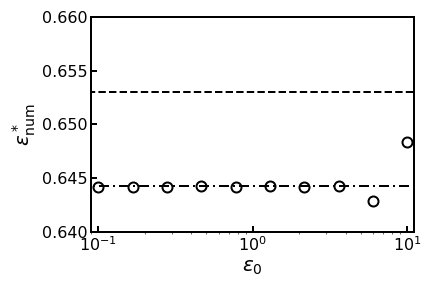
Figure 5: Numerically computed $\varepsilon_{\text{num}}^{*}$ vs. initial $\varepsilon_{0}$ (circles). Values are within $0.01\text{-}0.5\%$ of the numerical reference $\varepsilon_{\text{disc}}^{*}=0.64426$ (dash-dotted line) and within $1.3\%$ of the theoretical value $\varepsilon^{*}=0.653$ (dashed line).

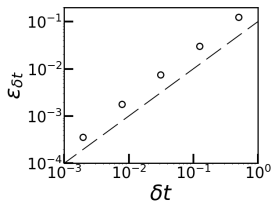
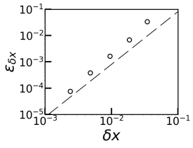
Figure 6: Convergence study with time step size (left, $\delta x=2.4\text{ mm}$) and with grid size (right, $\delta t=1.0\text{ ms}$). Dashed references lines are shown for first order on the left and for second order on the right.

V-B Pancake Flip

In this scenario, a Kinova JACO arm (6 DOF) is outfitted with a highly compliant Soft-bubble gripper [1]. The arm is anchored to a table which has a stand holding a spatula, a cylindrical stove top, and a pancake, modeled as a flat ellipsoid, on top. The Soft-bubble gripper and the pancake are modeled as compliant objects with hydroelastic modulus $E_{h}=10^{5}\text{ Pa}$ and $E_{h}=10^{4}\text{ Pa}$, respectively. Even though pancakes fold in reality, synthetic silicone pancakes were used in the real experimental setup, and therefore hydroelastic contact proved to be a useuful approximation. All remaining objects are modeled as rigid.

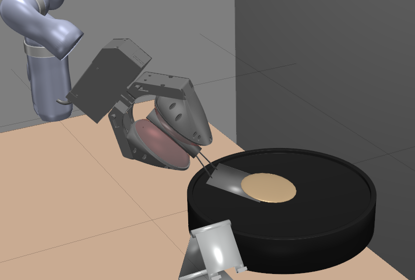
Figure 7: The scoop process of the pancake flip task. See associated video.

The controller process tracks a prescribed sequence of Cartesian end-effector keyframe poses. We use force feedback to gauge successful grasps and to know when the spatula makes contact with the stove top.

The robot is commanded to grab the spatula from the stand and subsequently scoop, raise, and flip the pancake over on the stove, see Fig. 7 and the accompanying supplemental video.

Figure 9 shows the number of faces throughout the simulation using both triangular and polygonal tessellations. On average, the number of faces is 4.05 times smaller when using the polygonal tessellation. Still, the model is able to resolve the net torque on the spatula needed to achieve a secure grasp. Moreover, with the resulting reduction in the number of contact constraints, our solver performs 4.09 times faster. The computation of polygonal tessellations is only about 10% faster than the corresponding triangular tessellations.

To assess scalability and task success at different grid sizes, we performed a grid refinement study using Drake’s SAP solver [21]. We used a system with 24 2.2 GHz Intel Xeon cores (E5-2650 v4) and 128 GB of RAM, running Linux. However we run in a single thread. We use the steady clock from the STL std::chrono library to measure wall-clock time. All grids use polygonal tessellations. Our coarsest grids result in 230 contacts per time step on average and we progressively refine grids by a factor of two, resulting in about 1500 constraints per time step on average, see the accompanying video. Figure 8 shows wall-clock time for the geometric queries and for the solver as a function of the average number of constraints per time-step.

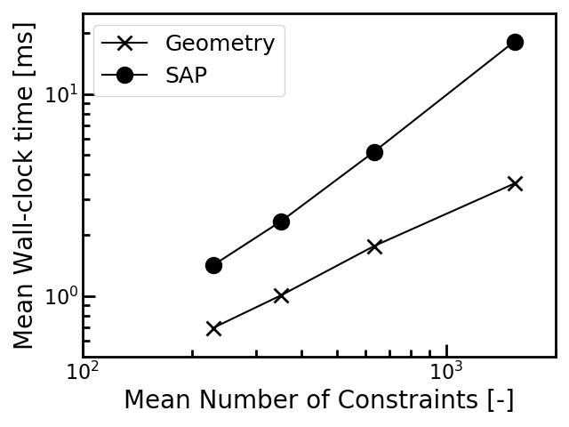
Figure 8: Mean wall-clock per time step vs. mean number of constraints per time step, for geometry and SAP solver.

We observe that the cost of the geometric queries is linear with the number of constraints (faces), demonstrating the effectiveness of OBBs as acceleration data structures in our implementation. For fully dense problems, we expect the solver to have $\mathcal{O}(n^{3})$ complexity, where $n$ denotes the number of variables. For sparse problems, the complexity is $\mathcal{O}(d^{3})$, where $d$ is the size of the largest clique in a chordal completion of the linear system matrix. A best fit exponent is about $\sim 1.3$ in Fig. 8, demonstrating the effectiveness of the supernodal algebra, even though this case is not very sparse.

For our coarsest set of grids, the spatula resembles a box rather than the original cylinder shape and the gripper uses a similarly coarse grid. Still, the robot completed the task successfully at all grid refinement levels. This demonstrates that the completion of this task in simulation is rather insensitive to mesh resolution.

Finally, our colleagues at TRI prototyped controllers in simulation that transferred seamlessly to the real robotic system, as shown in the accompanying video.

Figure 9: Number of faces generated as a function of time. Important events during the task are highlighted.

V-C Spatula Slip Control

We now demonstrate the effectiveness of our method to capture area-dependent phenomena such as the net torque required to successfully grasp an object. We simulate the aforementioned Soft-bubble gripper [1] anchored to the world holding a spatula by the handle horizontally. The grasp force is commanded to vary between $1\text{ N}$ and $16\text{ N}$ with square wave having a 6 second period and a 75% duty cycle, left on Fig. 10. This controller results in a periodic transition from a secure grasp with stiction to a loose grasp where the spatula is allowed to rotate within the grasp in a controlled manner, see Fig. 1 and the accompanying video.

Figure 1 (left) shows a closeup of the contact geometry used for this model. Notice that while well resolved, we use a rather coarse tessellation of the compliant bubble surfaces of the gripper. The polygonal tessellation provides a rich representation of the contact patch exhibited by an elongated shape induced by the geometry of the handle, Fig. 1 (right).

This level of grasp control is achieved by properly resolving contact patch area changes; this degree of control would be very difficult, if not impossible, to emulate using point contact approaches.

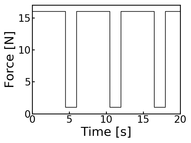
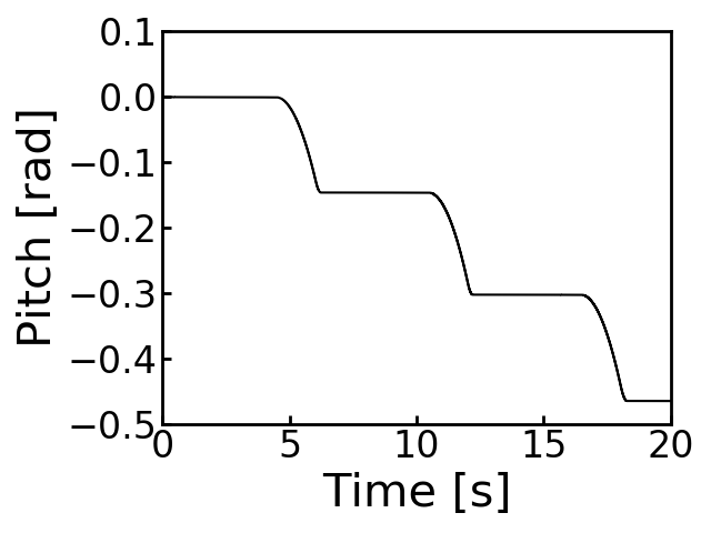
Figure 10: Commanded grasp force (left) and spatula pitch (right).

VI Limitations

All models are approximations of reality. We would like to explicitly state the limitations of our approach:

• Acceleration data structures and linear tetrahedra are key for a performant implementation of the hydroelastic contact model [11] for simulations at real time rates. Thus far, this limits the implementation to linear elements. Higher order elements or alternative representations are in interesting research direction.

• We show in Section IV that a single quadrature point located at the centroid of a polygon integrates the linear pressure field exactly. Conversely, moments are not integrated exactly. However, our method achieves second order accuracy with grid size as demonstrated with the grid study in Section V-A.

• The hydroelastic contact model is a modeling approximation which does not introduce deformation state. Therefore the model cannot resolve large deformations phenomena such as buckling or folding.

• Thin objects can be problematic. For instance, an equilibrium surface could not exit if a compliant thin box is pushed deep enough into a compliant half space. For this to happen the thin box needs to first get into such a configuration, which is possible especially for large time steps. We are currently working on ways to remedy this problem.

VII Conclusions

We presented a discrete in time approximation of the hydroelastic contact model to enable simulation of contact rich patches using velocity-level discrete solvers for simulation at real-time rates. The approach is general enough in that it can be incorporated into any velocity level solver that can handle compliant point contact.

We demonstrated the highly predictive nature of this model in a test case with strong coupling between net force and torque, matching known analytical results to within 1.3% without parameter tuning beyond choosing a mesh that can reasonably represent the geometry and choosing a time step that can resolve the temporal dynamics of the problem. Even though the polygonal tessellations are coarser than the original triangular tessellations from [11], we demonstrated the effectiveness of the approach to predict area-dependent phenomena such as the net torque required for the successful completion of a manipulation task.

Our novel surface representation in terms of polygonal faces leads to a drastic reduction in the number of contact constraints, a significantly smaller contact problem at each time step, and consequently a substantial speedup enabling simulation at interactive rates.

We present both time step size and grid size studies in order to assess the expected rate of convergence of our approximations. In particular, our method converges quadratically with grid size. The order of convergence with time step size depends on the particulars of the velocity level formulation, first order for our TAMSI [20] solver.

Finally, we include a mesh refinement study on the simulation of a real robotic task that involves grasping. The study reveals that the success of the task is not very sensitive to mesh resolution, even when using very coarse grids. Moreover, the study allowed us to assess the scalability of the contact queries and our SAP solver [21] with the number of constraints.

The hydroelastic contact model and the discrete approximation presented in this work are made available in the open-source robotics toolbox Drake [15]. The new model has been used extensively for work conducted at the Toyota Research Institute on prototyping and validating controllers for dexterous manipulation of complex geometries [31].

References

- [1] N. Kuppuswamy, A. Alspach, A. Uttamchandani, S. Creasey, T. Ikeda, and R. Tedrake, “Soft-bubble grippers for robust and perceptive manipulation,” in 2020 IEEE/RSJ International Conference on Intelligent Robots and Systems (IROS). IEEE, 2020, pp. 9917–9924.
- [2] E. Catto, “Soft constraints: Reinventing the spring,” Game Developer Conference, 2011.
- [3] L. Luo and M. Nahon, “A compliant contact model including interference geometry for polyhedral objects,” 2006.
- [4] Y. Gonthier, “Contact dynamics modelling for robotic task simulation,” 2007.
- [5] N. Wakisaka and T. Sugihara, “Loosely-constrained volumetric contact force computation for rigid body simulation,” in 2017 IEEE/RSJ International Conference on Intelligent Robots and Systems (IROS). IEEE, 2017, pp. 6428–6433.
- [6] E. Coumans, “SIGGRAPH 2015 course,” https://pybullet.org/wordpress/index.php/forum-2, 2015.
- [7] A. Moravanszky, P. Terdiman, and A. Kirmse, “Fast contact reduction for dynamics simulation,” Game programming gems, vol. 4, pp. 253–263, 2004.
- [8] K. Erleben, “Methodology for assessing mesh-based contact point methods,” ACM Transactions on Graphics (TOG), vol. 37, no. 3, pp. 1–30, 2018.
- [9] K. L. Johnson, Contact mechanics. Cambridge University Press, 1987.
- [10] M. A. Sherman, A. Seth, and S. L. Delp, “Simbody: multibody dynamics for biomedical research,” Procedia IUTAM, vol. 2, pp. 241–261, 2011.
- [11] R. Elandt, E. Drumwright, M. Sherman, and A. Ruina, “A pressure field model for fast, robust approximation of net contact force and moment between nominally rigid objects,” in 2019 IEEE/RSJ International Conference on Intelligent Robots and Systems (IROS). IEEE, 2019, pp. 8238–8245.
- [12] M. Macklin, K. Erleben, M. Müller, N. Chentanez, S. Jeschke, and Z. Corse, “Local optimization for robust signed distance field collision,” Proceedings of the ACM on Computer Graphics and Interactive Techniques, vol. 3, no. 1, pp. 1–17, 2020.
- [13] M. Tang, D. Manocha, M. A. Otaduy, and R. Tong, “Continuous penalty forces,” ACM Transactions on Graphics (TOG), vol. 31, no. 4, pp. 1–9, 2012.
- [14] M. Geilinger, D. Hahn, J. Zehnder, M. Bächer, B. Thomaszewski, and S. Coros, “Add: Analytically differentiable dynamics for multi-body systems with frictional contact,” ACM Transactions on Graphics (TOG), vol. 39, no. 6, pp. 1–15, 2020.
- [15] R. Tedrake and the Drake Development Team, “Drake: Model-based design and verification for robotics,” https://drake.mit.edu, 2019.
- [16] R. Smith, “Open dynamics engine,” http://www.ode.org.
- [17] J. Lee, M. X. Grey, S. Ha, T. Kunz, S. Jain, Y. Ye, S. S. Srinivasa, M. Stilman, and C. K. Liu, “Dart: Dynamic animation and robotics toolkit,” Journal of Open Source Software, vol. 3, no. 22, p. 500, 2018.
- [18] CM Labs Simulations, “Theory guide: Vortex software’s multibody dynamics engine,” https://www.cm-labs.com/vortexstudiodocumentation.
- [19] E. Todorov, “MuJoCo,” http://www.mujoco.org.
- [20] A. M. Castro, A. Qu, N. Kuppuswamy, A. Alspach, and M. Sherman, “A transition-aware method for the simulation of compliant contact with regularized friction,” IEEE Robotics and Automation Letters, vol. 5, no. 2, pp. 1859–1866, 2020.
- [21] A. Castro, F. Permenter, and X. Han, “An unconstrained convex formulation of compliant contact,” 2021, preprint available at https://arxiv.org/abs/2110.10107.
- [22] C. Lacoursiere and M. Linde, “Spook: a variational time-stepping scheme for rigid multibody systems subject to dry frictional contacts,” UMINF report, vol. 11, 2011.
- [23] D. E. Stewart, “Rigid-body dynamics with friction and impact,” SIAM review, vol. 42, no. 1, pp. 3–39, 2000.
- [24] A. Tasora and M. Anitescu, “A matrix-free cone complementarity approach for solving large-scale, nonsmooth, rigid body dynamics,” Computer Methods in Applied Mechanics and Engineering, vol. 200, no. 5-8, pp. 439–453, 2011.
- [25] M. Macklin, K. Erleben, M. Müller, N. Chentanez, S. Jeschke, and T.-Y. Kim, “Primal/dual descent methods for dynamics,” in Computer Graphics Forum, vol. 39, no. 8. Wiley Online Library, 2020, pp. 89–100.
- [26] M. Li, Z. Ferguson, T. Schneider, T. Langlois, D. Zorin, D. Panozzo, C. Jiang, and D. M. Kaufman, “Incremental potential contact: Intersection-and inversion-free, large-deformation dynamics,” ACM transactions on graphics, 2020.
- [27] Drake Development Team, “Hydroelastic contact user guide,” https://drake.mit.edu/doxygen˙cxx/group˙˙hydroelastic˙˙user˙˙guide.html.
- [28] D. E. Stewart and J. C. Trinkle, “An implicit time-stepping scheme for rigid body dynamics with inelastic collisions and coulomb friction,” International Journal for Numerical Methods in Engineering, vol. 39, no. 15, pp. 2673–2691, 1996.
- [29] M. Anitescu and F. A. Potra, “Formulating dynamic multi-rigid-body contact problems with friction as solvable linear complementarity problems,” Nonlinear Dynamics, vol. 14, no. 3, pp. 231–247, 1997.
- [30] Z. Farkas, G. Bartels, T. Unger, and D. E. Wolf, “Frictional coupling between sliding and spinning motion,” Physical review letters, vol. 90, no. 24, p. 248302, 2003.
- [31] R. Tedrake, “Drake: Model-based design in the age of robotics and machine learning,” https://medium.com/toyotaresearch/robotics/home, May 2021.