Energy preserving multiphase flows: Application to falling films.

Abstract

The numerical simulation of multiphase flows presents several challenges, namely the transport of different phases within de domain and the inclusion of capillary effects. Here, these are approached by enforcing a discrete physics-compatible solution. Extending our previous work on the discretization of surface tension [Valle2020] with a consistent mass and momentum transfer a fully energy-preserving multiphase flow method is presented. This numerical technique is showcased within the simulation of a falling film under several working conditions related to the normal operation of $\mathrm{LiBr}$ absorption chillers.

Keywords— Multiphase flows, Symmetry-preserving, Computational Methods, Falling films

1 INTRODUCTION

Vertical falling films are a canonical flow configuration which is inherently unstable even at $\mathrm{Re}=0$. When surface tension is present, the dynamics of such a system turn even more complex and interesting. Its application is of interest for many industrial applications in which high heat and mass transfer coefficients are expected with low temperature jumps. These include heat exchangers used in desalination and gas absorbers, like $\mathrm{HCl}$ absorbers used in chlorination processes and, most remarkably, $\mathrm{H_{2}O-LiBr}$ absorption chillers. The ultimate goal is to gain understanding on the instabilities appearing on this flow as a keystone to approach the heat and mass transfer processes in subsequent steps. In this regard, while the vapor phase has little effect in the fluid dynamics, it plays a key role when considering heat and mass transfer, in addition to ruling other non-linear phenomena such as the transport of volatile surfactant.

In the computational front, simulations of Nave et al. [2] replicated the experiments of Nosoko et al. [3] by using a ghost fluid - level set method and showed potential to capture flows transitioning from $2\mathrm{D}$ to $3\mathrm{D}$. The dominant role of inertia in governing the surface waves [4] has been studied by Denner et al. [5, 6], who performed remarkable experimental and numerical work. The role of capillary flow separation at increasing heat and mass transfer characteristics was assessed by Dietze and Kneer [7] from both experimental and numerical results, bolstering the role of surface tension at promoting heat and mass transfer in this flow configuration. Mass transfer enhancement at the capillary waves region was also confirmed by Bo et al. [8] in their $2\mathrm{D}$ simulation of a $\mathrm{H_{2}O-LiBr}$ absorber at $\mathrm{Re}=100$ and by Garcia-Rivera et al. [9].

Similarly, the work of Albert et al. [10] performed numerical simulations in order to asses the heat and mass transfer characteristics of falling films, which confirmed, again, the role of flow separation for the enhancement of such phenomenon. The study of $3\mathrm{D}$ structures in Dietze et al. [11] also observed flow separation. The assessment of corrugations and its impact in heat and mass transfer phenomena was also assessed by Dietze [12] for $\mathrm{Re}=15$.

In this context, the assessment of inertia and capillary terms, which rule the flow instabilities that promote heat and mass transfer, is of relevance for the development of new $\mathrm{H_{2}O-LiBr}$ absorbers. Nonetheless, the adoption of physically inconsistent schemes is customary for both convective and capillary terms. Accentuated by the high density ratios, this leads to inaccurate results and even numerical instabilities that compromise the accurate solution of the system. This highlights, once again, the importance of physics-compatible discretizations.

The simulation of multiphase flows in a fully physics-compatible way implies the conservation of discrete primary quantities (i.e., mass and momentum) and also secondary ones (i.e., mechanical energy) according to the physics described in the continuum. Two major obstacles prevent us from this: the inclusion of surface tension and the advection of a varying density flow.

In order to tackle these issues, symmetry-preserving ideas [13] have been used to set the mathematical grounds of the energy conservation in the context of fluid flow simulations. Those provide with a high degree of physical reliability, but also with improved stability.

Regarding the inclusion of surface tension, Fuster [14] developed on top of a Volume Of Fluid (VOF) method a discretization focusing on preserving the (skew-)symmetry of the operators involved, albeit overlooked surface tension, which is know to introduce spurious oscillations that may eventually lead to the divergence of the numerical simulation [15]. In the context of the level set method, our previous work resulted in the inclusion of curvature in an energy-preserving fashion [1], while the conservation of momentum is still elusive, a well known issue for diffuse interface models [16]. Within phase-field methods, the pioneering work of Jacqmin [17] included surface tension in a consistent way in the context of the Cahn-Hilliard equation. Phase-field methods success at capturing surface tension transfers between potential (elastic) and kinetic energy rely on taking the gradient of a surface potential, while VOF and level set methods aim at treating the usual curvature form.

The inclusion of a density-varying flow was tackled by Rudman [18] in the context of VOF by adopting a consistent mass and momentum transport scheme, which was focused on the simulation of multiphase flow with large density ratios. This approach was also adopted by Raessi and Pitch [19] and Ghods and Hermann [20] within the level-set method, while the work of Mirjalili and Mani [21] presented not only a consistent mass and momentum transport scheme, but also an energy-preserving scheme in the context of phase-field methods.

In this work, the framework of the well-known (mass) Conservative Level-Set method [22] is adopted for capturing the moving interface. Base on the energy-preserving level set method introduced in [1], we produce a fully energy-preserving method for multiphase flows by including a consistent mass and momentum transport as in Mirjalili and Mani [21]. Equipped with such a physics-compatible discretization, we target DNS of vertical falling films.

The rest of the paper is organized as follows: in section 2 the governing equations are introduced, in section 3 the numerical method is detailed, while in section 4 the cases under consideration are introduced and the results commented. Finally, in section 5 conclusions are drawn and future developments sketched.

2 MATHEMATICAL MODEL

The subtle physical equilibrium at which the fluid system is subject calls for a careful, and thus conservative, formulation of the governing equations.

The interface separating the two phases is modeled implicitly by means of a marker function $\theta\in[0,1]$ which can be regularized as needed, as will be discussed in next section. The values $\theta=0$ indicate the liquid phase, $\theta=1$ corresponds with the gaseous one and $\theta=0.5$ with the interface location. For a sufficiently well-behaved $\theta$, the interface normal is defined as

$$\hat{\eta}_{i}=\frac{\nabla\theta}{|\nabla\theta|}$$ (1)

while the interface curvature is defined as

$$\kappa=\nabla\cdot\hat{\eta}_{i}$$ (2)

Note that when the marker function is the distance function, $|\nabla\theta|=1$ and thus $\hat{\eta}_{i}=\nabla\theta$.

The flow is assumed incompressible for both liquid and gaseous phases

$$\nabla\cdot\vec{u}=0$$ (3)

under this assumption, the marker function obeys the following transport equation

$$\frac{\partial\theta}{\partial t}+\nabla\cdot\left(\vec{u}\theta\right)=0$$ (4)

while the momentum transport is ruled by the conservative version of the dimensionless Navier-Stokes equations. Exploiting the Nusselt flat film solution we introduce Reynolds ($\mathrm{Re}$) and Weber ($We$) numbers. Additionally, because we are concerned with the solution of both liquid and gaseous phases simultaneously, we introduce density ($\Pi_{\rho}=\rho_{g}/\rho_{l}$) and viscosity ($\Pi_{\mu}=\mu_{g}/\mu_{l}$) ratios. Accordingly, we consider the non-dimensional versions of density ($X_{\rho}=\rho/\rho_{l}\in[1,\Pi_{\rho}]$) and viscosity ($X_{\mu}=\mu/\mu_{l}\in[1,\Pi_{\mu}]$). We finally end up with the following momentum equation

$$3\mathrm{Re}\left(\frac{\partial\left(X_{\rho}\vec{u}\right)}{\partial t}+\nabla\cdot\left(X_{\rho}\vec{u}\otimes\vec{u}\right)\right)=-\nabla p+\nabla\cdot 2X_{\mu}S+X_{\rho}\hat{g}$$ (5)

subject to capillary forces at the interface, which impose a stress discontinuity, $\left[\sigma\right]$ as

$$\left[\sigma\right]\hat{\eta}_{i}=-We\kappa\hat{\eta}_{i}$$ (6)

being $\sigma=-p\mathbb{I}+\mu S$ the stress tensor, $S=1/2\left(\nabla\vec{u}+(\nabla\vec{u})^{T}\right)$ the strain tensor and $\hat{g}=(0,-1,0)$.

Which introduce the following dimensionless parameters

$$\mathrm{Re} =\frac{\rho_{l}u_{N}h_{N}}{\mu_{l}}$$ (7)

$$We =\frac{\gamma}{\rho_{l}u_{N}h_{N}^{2}}$$ (8)

being $h_{N}$ the undisturbed film thickness and $u_{N}$ the mean liquid velocity. The domain under consideration is assumed to be periodic in both $y$ and $z$ directions, while solid walls are present in the $x$ direction. In a symmetric setup with respect to the $x$ mid-plane, there is a film flowing down each wall.

No-slip velocity

$$\vec{u}\rvert_{wall}=\vec{0}$$ (9)

and no marker flow

$$\nabla\theta\cdot\hat{n}\rvert_{wall}=0$$ (10)

are prescribed at both solid walls.

3 NUMERICAL METHOD

3.1 Discretization

We proceed as in [1] by discretizing differential geometry operators from a geometrical perspective and then construct discrete vector calculus operators within a finite volume method. Once we obtain the discrete versions of the differential geometry operators, we construct the discrete counterparts of divergence ($\mathsf{D}_{\mathsf{}}$), gradient ($\mathsf{G}_{\mathsf{}}$), Laplacian ($\mathsf{L}_{\mathsf{}}$) and convective ($\mathsf{C}(\cdot)_{\mathsf{}}$) operators, resulting in a classical finite volume, second order, staggered method as introduced by Harlow and Welch [23, 13]. In addition, we introduce a high resolution advection schemes ($\mathsf{C}(\mathbf{{u}_{f}})_{\mathsf{}}$) via flux limiters in a similar fashion [24].

After adopting a proper regularization, we introduce the following equations for the physical properties

$$\mathbf{{\uprho}_{f}} =1+\left(\Pi_{\rho}-1\right)\mathbf{{\uptheta}_{f}}$$ (11)

$$\mathbf{{\upmu}_{f}} =1+\left(\Pi_{\mu}-1\right)\mathbf{{\uptheta}_{f}}$$ (12)

while the original set of governing equations (3-5) is discretized as

$$\mathsf{D}_{\mathsf{}}\mathbf{{u}_{f}} =\mathbf{0_{{c}}}$$ (13)

$$\frac{d\mathbf{{\uptheta}_{c}}}{dt} =-\mathsf{C}(\mathbf{{u}_{f}})_{\mathsf{}}\mathbf{{\uptheta}_{c}}$$ (14)

$$3\mathrm{Re}\frac{d\left(\mathsf{P}\mathbf{{u}_{f}}\right)}{dt} =-\mathsf{C}(\mathsf{P}\mathbf{{u}_{f}})_{\mathsf{}}\mathbf{{u}_{f}}-\mathsf{G}_{\mathsf{}}\mathbf{{p}_{c}}+\mathsf{L}_{\mathsf{}}\mathbf{{u}_{f}}+We~{}\mathsf{K_{F}}\mathsf{G}_{\mathsf{}}\mathbf{{\uptheta}_{c}}+\mathsf{P}\mathbf{g}$$ (15)

where $\mathbf{{u}_{f}}$ stands for the staggered velocity field, $\mathbf{{\uptheta}_{c}}$ is the collocated marker function and $\mathbf{{p}_{c}}$ the collocated pressure, $\mathsf{P}=\mathsf{diag}\left(\mathbf{{\uprho}_{f}}\right)$ is the diagonal matrix arrangement of the staggered density, and $\mathsf{K_{F}}=\mathsf{diag}\left({\Upsilon}\mathbf{{k}_{c}}\right)$ is the diagonal arrangement of the staggered curvature that was introduced in Valle et al. [1].

The conservation of mass is a consequence of the conservation of the marker function stated in equation (14) and the linear reconstruction of density as in equation (11)

$$\frac{d\mathbf{{\uprho}_{c}}}{dt}=(\rho_{1}-\rho_{0})\frac{d\mathbf{{\uptheta}_{c}}}{dt}=-(\rho_{1}-\rho_{0})\mathsf{C}(\mathbf{{u}_{f}})_{\mathsf{}}\mathbf{{\uptheta}_{c}}=-\mathsf{C}(\mathbf{{u}_{f}})_{\mathsf{}}\mathbf{{\uprho}_{c}}$$ (16)

which it is implicitly defined by means of equations (11) and (14).

3.2 Conservation of energy

The evolution of kinetic energy $E_{k}=1/2\left(\rho\vec{u},\vec{u}\right)_{\mathsf{}})$ for multiphase flows is discussed by first analyzing the conservation of energy in terms of the velocity field $\vec{u}$ and the conservative equations (16) and (15) as in [21]

$$\frac{dE_{k}}{dt}=\frac{1}{2}\left(\vec{u},\frac{\partial\left(\rho\vec{u}\right)}{\partial t}\right)_{\mathsf{}}+\frac{1}{2}\left(\rho\vec{u},\frac{\partial\vec{u}}{\partial t}\right)_{\mathsf{}}=\left(\vec{u},\frac{\partial\left(\rho\vec{u}\right)}{\partial t}\right)_{\mathsf{}}-\frac{1}{2}\left(\vec{u},\vec{u}\frac{\partial\rho}{\partial t}\right)_{\mathsf{}}$$ (17)

where we have included the inner product $\left(f,g\right)_{\mathsf{}}=\int fgdV$, which applies to both continuous and discrete fields. We then obtain the discrete counterpart of equation equation (17) by including equations (15) and (16), the former requiring the use of the isometric cell-to-face interpolation operator $\Pi$ in order to match dimensions of the discrete field. After rearranging terms, we obtain

$$\frac{d\mathbf{{E_{k}}}}{dt}=\frac{d\left(\mathbf{{u}_{f}},\mathsf{P}\mathbf{{u}_{f}}\right)_{\mathsf{}}}{dt}= -\left(\mathbf{{u}_{f}},\mathsf{C}(\mathsf{P}\mathbf{{u}_{f}})_{\mathsf{}}\mathbf{{u}_{f}}\right)_{\mathsf{}}+\left(\mathbf{{u}_{f}},\mathsf{G}_{\mathsf{}}\mathbf{{p}_{c}}\right)_{\mathsf{}}+\left(\mathbf{{u}_{f}},\mathsf{L}_{\mathsf{}}\mathbf{{u}_{f}}\right)_{\mathsf{}}+We\left(\mathbf{{u}_{f}},\mathsf{K_{F}}\mathsf{G}_{\mathsf{}}\mathbf{{\uptheta}_{c}}\right)_{\mathsf{}}+\left(\mathbf{{u}_{f}},\mathsf{P}\mathbf{g}\right)_{\mathsf{}}$$ (18)

$$+\frac{1}{2}\left(\mathbf{{u}_{f}},\mathsf{U}\Pi\mathsf{C}(\mathbf{{u}_{f}})_{\mathsf{}}\mathbf{{\uprho}_{c}}\right)_{\mathsf{}}$$

where $\mathsf{U}=diag\left(\mathbf{{u}_{f}}\right)$ is the diagonal arrangement of the staggered velocity field. Note that the discrete inner product takes the form of a weighted vector dot product, i.e., $\left(\mathbf{{u}_{f}},\mathsf{P}\mathbf{{u}_{f}}\right)_{\mathsf{}}=\mathbf{{u}_{f}}^{T}\mathsf{V_{f}}\mathsf{P}\mathbf{{u}_{f}}$, where $\mathsf{V_{f}}=diag(v_{f})$ is the diagonal arrangement of the staggered volumes. We have also included the implicit version of the mass transfer equations, even when, as it was discussed above, this equation is not explicitly computed.

We now analyze the evolution of potential energy,

$$\frac{dE_{p}}{dt}=-We\left(\vec{u},\kappa\nabla\theta\right)_{\mathsf{}}-\left(\vec{u},X_{\rho}\vec{g}\right)_{\mathsf{}}$$ (19)

which is composed of the capillary and the buoyancy term. Analogously, the evolution of discrete potential energy equation is obtained in an analogous way as in equation (19)

$$\frac{d\mathbf{{E_{p}}}}{dt}=-We\left(\mathbf{{u}_{f}},\mathsf{K_{F}}\mathsf{G}_{\mathsf{}}\mathbf{{\uptheta}_{c}}\right)_{\mathsf{}}-\left(\mathbf{{u}_{f}},\mathsf{P}\mathbf{g}\right)_{\mathsf{}}$$ (20)

where we have adopted an energy-preserving discretization of the capillary terms as we did in [1].

Finally, we are now able to assess the evolution of discrete mechanical energy by including equations (18) and (20). After rearranging, we obtain

$$\frac{d\mathbf{{E_{m}}}}{dt}=-\left(\mathbf{{u}_{f}},\mathsf{C}(\mathsf{P}\mathbf{{u}_{f}})_{\mathsf{}}\mathbf{{u}_{f}}\right)_{\mathsf{}}+\frac{1}{2}\left(\mathbf{{u}_{f}},\mathsf{U}\Pi\mathsf{C}(\mathbf{{u}_{f}})_{\mathsf{}}\mathbf{{\uprho}_{c}}\right)_{\mathsf{}}+\left(\mathbf{{u}_{f}},\mathsf{L}_{\mathsf{}}\mathbf{{u}_{f}}\right)_{\mathsf{}}<0$$ (21)

where the pressure terms has vanished given that $\mathsf{D}_{\mathsf{}}\mathbf{{u}_{f}}=0$, as shown in [13].

We are, however, left with the two first convective terms in equation (21) which should, in virtue of its convective nature, ideally vanish. From this point onward, we follow Mirjalili and Mani [21] to show that the adoption of a consistent mass and momentum transport along with a smart interpolation strategy results in an energy-consistent discretization. To do so, we note first that the momentum convective operator is not skew-symmetric due to $\mathsf{D}_{\mathsf{}}\mathsf{P}\mathbf{{u}_{f}}\neq 0$ if density is not constant. However, due to the mimetic structure adopted for the construction of $\mathsf{C}(\cdot)_{\mathsf{}}$, we can decompose $\mathsf{C}(\mathsf{P}\mathbf{{u}_{f}})_{\mathsf{}}$ as

$$\mathsf{C}(\mathsf{P}\mathbf{{u}_{f}})_{\mathsf{}}=\mathsf{C}^{off}(\mathsf{P}\mathbf{{u}_{f}})_{\mathsf{}}+\frac{1}{2}diag\left(\Pi\mathsf{D}_{\mathsf{}}\mathsf{P}\mathbf{{u}_{f}}\right)$$ (22)

The off-diagonal part $\mathsf{C}^{off}(\mathsf{P}\mathbf{{u}_{f}})_{\mathsf{}}$ is a purely skew-symmetric operator, which results into an energy neutral operator, and we are left with the diagonal one $1/2diag\left(\Pi\mathsf{D}_{\mathsf{}}\mathsf{P}\mathbf{{u}_{f}}\right)$, where the $1/2$ factor arise from the interpolation applied to the transported velocity field [13].

Introducing equation (22) into equation (21) we obtain

$$\frac{d\mathbf{{E_{m}}}}{dt}=-\frac{1}{2}\left(\mathbf{{u}_{f}},diag\left(\Pi\mathsf{D}_{\mathsf{}}\mathsf{P}\mathbf{{u}_{f}}\right)\mathbf{{u}_{f}}\right)_{\mathsf{}}+\frac{1}{2}\left(\mathbf{{u}_{f}},\mathsf{U}\Pi\mathsf{C}(\mathbf{{u}_{f}})_{\mathsf{}}\mathbf{{\uprho}}\right)_{\mathsf{}}+\left(\mathbf{{u}_{f}},\mathsf{L}_{\mathsf{}}\mathbf{{u}_{f}}\right)_{\mathsf{}}$$ (23)

then, exploiting $\mathsf{A}\mathbf{{b}}=diag(\mathbf{{a}})\mathbf{{b}}=diag(\mathbf{{b}})\mathbf{{a}}=\mathsf{B}\mathbf{{a}}$ to rearrange $diag\left(\Pi\mathsf{D}_{\mathsf{}}\mathsf{P}\mathbf{{u}_{f}}\right)\mathbf{{u}_{f}}=\mathsf{U}\Pi\mathsf{D}_{\mathsf{}}\mathsf{P}\mathbf{{u}_{f}}$ first and $\mathsf{P}\mathbf{{u}_{f}}=\mathsf{U}\mathbf{{\uprho}_{f}}$ later, we obtain

$$\frac{d\mathbf{{E_{m}}}}{dt} =-\frac{1}{2}\left(\mathbf{{u}_{f}},\mathsf{U}\Pi\mathsf{D}_{\mathsf{}}\mathsf{U}\mathbf{{\uprho}_{f}}\right)_{\mathsf{}}+\frac{1}{2}\left(\mathbf{{u}_{f}},\mathsf{U}\Pi\mathsf{C}(\mathbf{{u}_{f}})_{\mathsf{}}\mathbf{{\uprho}_{c}}\right)_{\mathsf{}}+\left(\mathbf{{u}_{f}},\mathsf{L}_{\mathsf{}}\mathbf{{u}_{f}}\right)_{\mathsf{}}$$ (24)

We then introduce the definition $\mathsf{C}(\mathbf{{u}_{f}})_{\mathsf{}}=\mathsf{D}_{\mathsf{}}\mathsf{U}\Psi$ introduced in [24, 1], where $\Psi$ contains the high resolution cell-to-face interpolation, to yield

$$\frac{d\mathbf{{E_{m}}}}{dt} =-\frac{1}{2}\left(\mathbf{{u}_{f}},\mathsf{U}\Pi\mathsf{D}_{\mathsf{}}\mathsf{U}\mathbf{{\uprho}_{f}}\right)_{\mathsf{}}+\frac{1}{2}\left(\mathbf{{u}_{f}},\mathsf{U}\Pi\mathsf{D}_{\mathsf{}}\mathsf{U}\Psi\mathbf{{\uprho}_{c}}\right)_{\mathsf{}}+\left(\mathbf{{u}_{f}},\mathsf{L}_{\mathsf{}}\mathbf{{u}_{f}}\right)_{\mathsf{}}$$ (25)

from where we can infer the proper cell-to-face interpolation for the discrete density field as

$$\mathbf{{\uprho}_{f}}=\Psi\mathbf{{\uprho}_{c}}$$ (26)

such that convective contributions to the discrete mechanical energy cancel out and finally yield

$$\frac{d\mathbf{{E_{m}}}}{dt}=\left(\mathbf{{u}_{f}},\mathsf{L}_{\mathsf{}}\mathbf{{u}_{f}}\right)_{\mathsf{}}<0$$ (27)

Note, however, that $\mathbf{{\uprho}_{c}}$ is actually not computed but can easily be obtained from $\mathbf{{\uptheta}_{f}}$ as

$$\mathbf{{\uprho}_{f}}=\rho_{0}+(\rho_{1}-\rho_{0})\mathbf{{\uptheta}_{f}}$$ (28)

stating an explicit relationship between the advection of the marker function and the reconstruction of density. This was previously introduced in the literature, along with other specific techniques, as consistent mass and momentum transport [18, 19, 20, 21]. In summary, we have developed a consistent discretization that can easily preserve mass, momentum (up to surface tension) and energy.

Following the original work of Rudman [18], the adoption of the FSM method can proceed with slight modifications. We adopt the LU decomposition approach introduced by Perot [25] in order to show the integration procedure of an explicit time integration scheme and the modification with respect to the classical FSM followed by Rudman [18]. First, following the conservative nature of the governing, equations, we will integrate in time discrete momentum i.e., considering $(\mathsf{P}\mathbf{{u}_{f}})$ as variable on its own. Second, we will use the new density and momentum fields in order to obtain a new velocity field which is consistent with the former two.

The semi-discretized equations (14) and (15) can be compiled together with the velocity-momentum expression and the usual divergence free constrain $\mathsf{D}_{\mathsf{}}\mathbf{{u}_{f}}=0$ to result in a linear system of equations as

$$\begin{pmatrix}d_{t}&0&0&0\\ 0&d_{t}&0&\mathsf{G}_{\mathsf{}}\\ 0&\mathsf{I_{f}}&-\mathsf{P}&0\\ 0&0&\mathsf{D}_{\mathsf{}}&0\\ \end{pmatrix}\begin{pmatrix}\mathbf{{\uptheta}_{c}}\\ \mathsf{P}\mathbf{{u}_{f}}\\ \mathbf{{u}_{f}}\\ \mathbf{{p}_{c}}\\ \end{pmatrix}=\begin{pmatrix}-\mathsf{C}(\mathbf{{u}_{f}})_{\mathsf{}}\mathbf{{\uptheta}_{c}}\\ \mathsf{R}(\mathbf{{\uprho}_{f}}^{n},\mathbf{{u}_{f}}^{n},\mathbf{{p}_{c}}^{n})\\ \mathbf{0_{{f}}}\\ \mathbf{0_{{c}}}\\ \end{pmatrix}$$ (29)

where $\mathsf{R}(\mathbf{{\uprho}_{f}}^{n},\mathbf{{u}_{f}}^{n},\mathbf{{p}_{c}}^{n})=-\mathsf{C}(\mathsf{P}^{n}\mathbf{{u}_{f}}^{n})_{\mathsf{}}\mathbf{{u}_{f}}^{n}-\mathsf{L}_{\mathsf{}}\mathbf{{u}_{f}}^{n}+We\mathsf{K}^{n}\mathsf{G}_{\mathsf{}}\mathbf{{\uptheta}_{c}}^{n}+\mathsf{P}^{n}\mathbf{g}$ corresponds with a generalized explicit treatment of the right hand side of equation (15) without the pressure term. Note that the left-hand-side is evaluated at time level $n+1$, while the right hand side is evaluated at $n$ (or, in general, previous time-steps). In an explicit setup as the one described here, this implies that the density field used for the momentum transport (2nd row) is evaluated at time level $n$, whereas the density field used to impose the divergence-free velocity field is evaluated at time level $n+1$. We can then perform an LU decomposition as

$$\begin{pmatrix}d_{t}&0&0&0\\ 0&d_{t}&0&\mathsf{G}_{\mathsf{}}\\ 0&\mathsf{I_{f}}&-\mathsf{P}&0\\ 0&0&\mathsf{D}_{\mathsf{}}&0\\ \end{pmatrix}=\begin{pmatrix}d_{t}&0&0&0\\ 0&d_{t}&0&0\\ 0&\mathsf{I_{f}}&-\mathsf{P}&0\\ 0&0&\mathsf{D}_{\mathsf{}}&-\frac{1}{d_{t}}\mathsf{D}_{\mathsf{}}\mathsf{P}^{-1}\mathsf{G}_{\mathsf{}}\\ \end{pmatrix}\begin{pmatrix}\mathsf{I_{c}}&0&0&0\\ 0&\mathsf{I_{f}}&0&\frac{1}{d_{t}}\mathsf{G}_{\mathsf{}}\\ 0&0&\mathsf{I_{f}}&\frac{1}{d_{t}}\mathsf{P}^{-1}\mathsf{G}_{\mathsf{}}\\ 0&0&0&\mathsf{I_{c}}\\ \end{pmatrix}$$ (30)

From here, the modified FSM algorithm follows by the usual solution of the system by $\mathsf{LU}$ inversion. We finally obtain the resulting algorithm as

1	Integrate	$\frac{d\mathbf{{\uptheta}_{c}}}{dt}$	$=-\mathsf{C}(\mathbf{{u}_{f}})_{\mathsf{}}\mathbf{{\uptheta}_{c}}^{n}$	$\to\mathbf{{\uptheta}_{c}}^{n+1}$
2	Integrate	$\frac{d\left(\mathsf{P}\mathbf{{u}_{f}}\right)}{dt}$	$=\mathsf{R}(\mathbf{{\uprho}_{f}}^{n},\mathbf{{u}_{f}}^{n},\mathbf{{p}_{c}}^{n})$	$\to\left(\mathsf{P}\mathbf{{u}_{f}}\right)^{\star}$
3	Solve	$\mathsf{P}^{n+1}\mathbf{{u}_{f}}^{\star}$	$=\left(\mathsf{P}\mathbf{{u}_{f}}\right)$	$\to\mathbf{{u}_{f}}^{\star}$
4	Solve	$\mathsf{D}_{\mathsf{}}\mathsf{P}^{-1}\mathsf{G}_{\mathsf{}}\mathbf{{p}_{c}}^{n+1}$	$=\mathsf{D}_{\mathsf{}}\mathbf{{u}_{f}}^{\star}$	$\to\mathbf{{p}_{c}}^{n+1}$
5	Correct	$\mathbf{{u}_{f}}^{n+1}$	$=\mathbf{{u}_{f}}^{\star}-\frac{1}{dt}\mathsf{P}^{-1}\mathsf{G}_{\mathsf{}}\mathbf{{p}_{c}}$	$\to\mathbf{{u}_{f}}^{n+1}$
6	Update	$\left(\mathsf{P}\mathbf{{u}_{f}}\right)^{n+1}$	$=\mathsf{P}^{n+1}\mathbf{{u}_{f}}^{n+1}$	$\to\left(\mathsf{P}\mathbf{{u}_{f}}\right)^{n+1}$

Algorithm 1 Integration of the governing equations along a Fractional Step Method as in [18]

where we have we have re-stated the computation of the $\left(\mathsf{P}\mathbf{{u}_{f}}\right)^{n+1}$ in the equivalent form of step $6$ to reassert that the new momentum field is consistent with the divergence-free velocity and density fields. We have also redefined pressure to include time integration, as it is customary.

4 PRELIMINARY RESULTS

With the aforementioned discretization in mind, we showcase the proposed DNS discretization of the system with the simulation of several falling films. Introducing the Kapitza number

$$Ka=\frac{\gamma}{\rho_{l}^{1/3}\mu_{l}^{4/3}}$$ (31)

we obtain a dimensionless number that is fixed with the physical properties of the working liquid, while the density ($\Pi_{\rho}$) and viscosity ($\Pi_{\mu}$) ratios provide with the information regarding the vapor phase. In this manner, the liquid-gas pair properties can be fully described by $Ka$, $\Pi_{\rho}$ and $\Pi_{\mu}$, as seen in Table1, while $\mathrm{Re}$ is left as the solely variable controlling the fluid dynamics of the system, which i set at $Re=\{150,200\}$ to define typical falling film dynamics involved in absorption chillers.

id	fluid	$T(^{\circ}C)$	$X_{abs}$	$Ka$	$\Pi_{\rho}(\times 10^{-3})$	$\Pi_{\mu}(\times 10^{-3})$
$A$	$H_{2}O$	$9.9$	$0.00$	$2420$	$0.60$	$9.37$
$B$	$H_{2}O/LiBr$	$50.0$	$0.60$	$443$	$0.35$	$2.45$
$C$	$H_{2}O/Carrol$	$50.0$	$0.67$	$150$	$0.35$	$1.10$

Table 1: Estimated fluid properties dimensionless groups. For three typical working fluids in an absorption chiller.

The computational domain is a $[10h_{N}\times\Lambda_{y}\times\Lambda_{z}]$ box with periodic boundaries in both $y$ and $z$ directions, where $\Lambda_{y}=\Lambda_{x}=100h_{N}$, which correspond with the length of a long-wave perturbation. We will denote $x$, $y$ and $z$ directions as wall-normal, stream-wise and span-wise, and $N_{x}$, $N_{y}$ and $N_{z}$ the number of nodes in the $x$, $y$ and $z$ directions. The mesh is refined in the vicinity of the flat film thickness and coarsened at the center of the box, where the gas phase is expected. The following expression gives the refinement introduced in the $x$ axis

$$x =L_{x}\left(0.5f_{x}\left(1+\frac{sinh\left(\alpha\left(\frac{i}{N_{r}}-0.5\right)\right)}{sinh\left(\frac{\alpha}{2}\right)}\right)\right) \forall i\in[0,N_{r}]$$ (32)

$$x =L_{x}\left(f_{x}+0.5(1-2f_{x})\left(1+\frac{tanh\left(\beta\frac{i-N_{r}}{N_{x}-2N_{r}}-0.5\right)}{tanh\left(\frac{\beta}{2}\right)}\right)\right) \forall i\in[N_{r},N_{x}-N_{r}]$$

$$x =L_{x}\left((1-f_{x})+0.5f_{x}\left(1+\frac{sinh\left(\alpha\frac{i-N_{x}+N_{r}}{N_{r}}-0.5\right)}{sinh\left(\frac{\alpha}{2}\right)}\right)\right) \forall i\in[N_{x}-N_{r},N_{x}]$$

where $L_{x}=10$, $f_{x}=0.2$ is the fraction of $L_{x}$ refined close to the wall, while $N_{r}=N_{x}/3$ is the number of nodes introduced in the refinement regions. Parameters $\alpha=2$ and $\beta=2$ control the smoothness of the refinements.

We set up a symmetric layout consisting of two films falling down parallel walls. The interface is initialized as in Dietze et al. [11] by prescribing a perturbation at the film surface as

$$h=h_{N}\left(1+\epsilon_{y}cos\left(2\pi\frac{y}{\Lambda_{y}}\right)+\epsilon_{z}cos\left(2\pi\frac{z}{\Lambda_{z}}\right)\right)$$ (33)

where $h$ is the perturbed film thickness, $\epsilon_{y}=0.2$ and $\epsilon_{z}=0.05$ are chosen according to Dietze et al. [11] and correspond with amplitude of the perturbation in the $y$ and $z$ directions, respectively. The wavelength $\Lambda_{y}$ and $\Lambda_{z}$ are sufficiently large to represent long-wave perturbations [4] and the velocity profile is initialized to the undisturbed flat falling film solution.

Time integration is performed with a 3rd order Runge-Kutta method for step $1$ and a 2nd order Adams-Bashforth one for step $2$. The solver used for the Poisson equation is a Preconditioned Conjugate Gradient (PCG) method preconditioned with $\mathsf{P}$ in order to reduce the condition number of the system.

Results shown in figures 1 and 2 show the impact of decreasing Kapitza number into the dynamics of the surface. The stabilizing effect of surface tension fades as the Kapitza number is reduced, thus enhancing the appearance of larger humps and complex instabilities.

In this regard, results show the appearance of a leading depression before the arrival of the wave tip, which drains fluid in the $z$ direction, which contributes to the appearance of $3D$ structures as shown in [11]. This depression is more pronounced in the low Kapitza cases due to the stabilizing effect that capillary force plays in the development of surface deformations. While the stiffer case $A$ presents a less marked curvature, it also presents more undulations on the film surface. This results in the appearance of a more dispersed velocity field on top of the film surface. Conversely, lower Kapitza numbers result in more acute film deformations, which, on the other hand, contribute to smaller, but also more coherent, flow patterns.

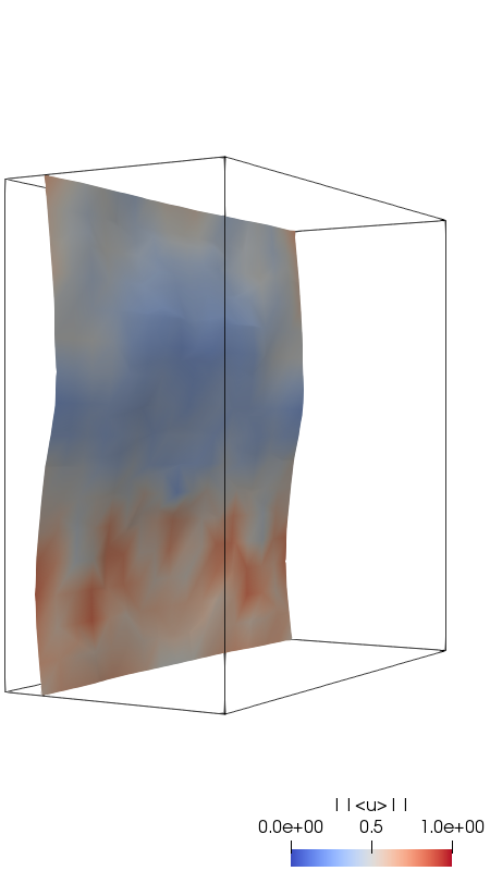
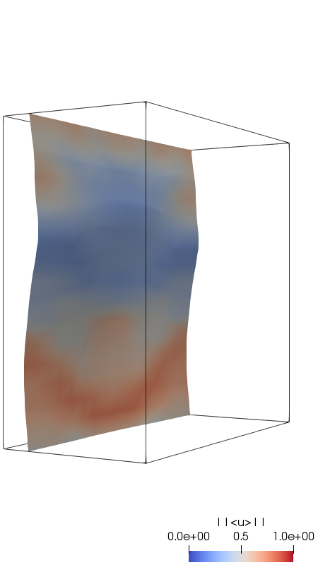
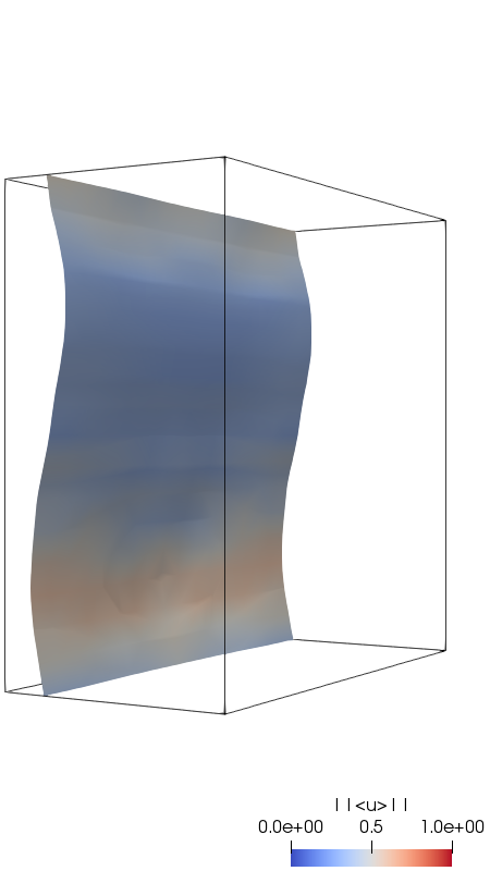
Figure 1: Velocity magnitude on the film surfaces for cases $A$, $B$ and $C$ at $\mathrm{Re}=150$ after $T=100$.

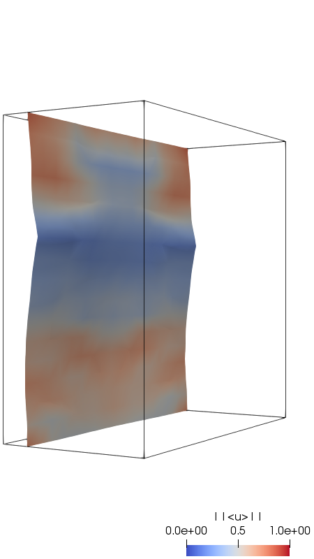
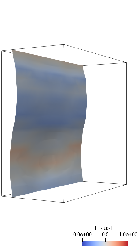
Figure 2: Velocity magnitude on the film surfaces for cases $A$, $B$ and $C$ at $\mathrm{Re}=200$ after $T=100$.

Regarding the shape of the film interface, it can be observed how case $B$ produces a more abrupt hump, showing a marked preceding wave rise and a also a central delay on wave maximum, pushing the flow in the $z$ direction and thus revealing the incipient formation of a horseshoe pattern. On the other hand, milder surface effects in case $C$ result in a smoother undulation, which show smaller $z$ axis flow which is mainly in the $y$ direction. These effects are intensified with the increase of the Reynolds number, as it can be seen for case $B$ at $\mathrm{Re}=200$. In that situation, the wave is rolling on top of itself thus increasing the hump height an resulting into a growing large scale instability. On the other hand, the high Kapitza case presented in case $A$ shows milder velocity fields at higher Reynolds numbers, which may caused by an intensified momentum diffusion at the interface due to the high frequency pattern that the undulations on top of the surface form.

5 CONCLUSIONS

The method has been deployed in the DNS of vertical falling films under extreme density ratios, which pose a major numerical challenge and at the same time are of industrial relevance. Results are in accordance with the expected behavior of such films and reported in both experimental and numerical literature. In this regard, it is shown capillary forces stabilizing effect on the film dynamics. Accordingly, reducing surface tension (e.g., by adding surfactants) is observed to enhance instability of the system.

Extending our previous work on the energy-preserving inclusion of curvature [1] and adopting the ideas presented in Mirjalili and Mani [21] for the discretization of the convective terms, we present a formulation which is mathematically consistent. The aforementioned merits benefit from the adoption of our heavily algebra-based formulation both for the discretization and the formulation of the modified FSM as proposed by Rudman [18], revealing the close connection between consistent mass and momentum transfer and the conservation of energy.

While we succeeded at the formulation of a fully mass conservative and energy-preserving scheme, the conservation of linear momentum is still unclear [16]. However, as it was already commented in [1], while the lack of total momentum conservation is an undesired property, the adoption of an energy-preserving scheme provides a bound on total energy and thus stability. Nonetheless, the conservation of linear momentum is an active line of research that deserves further discussion.

References

- [1] N. Valle, F. X. Trias, and J. Castro. An energy-preserving level set method for multiphase flows. J. Comput. Phys., 400:108991, 2020.
- [2] J.-C. Nave, X. D. Liu, and Sanjoy Banerjee. Direct Numerical Simulation of Liquid Films with Large Interfacial Deformation. Stud. Appl. Math., pages 153–177, 2010.
- [3] C. D. Park and T. Nosoko. Three-Dimensional Wave Dynamics on a Falling Film and Associated Mass Transfer. AIChE J., 49(11):2715–2727, 2003.
- [4] S. Kalliadasis, C. Ruyer-Quil, B. Scheid, and M. G. Velarde. Falling Liquid Films, volume 176. Springer, London, 2012.
- [5] Fabian Denner, Marc Pradas, Alexandros Charogiannis, Christos N. Markides, Berend G. M. van Wachem, and Serafim Kalliadasis. Self-similarity of solitary waves on inertia-dominated falling liquid films. Phys. Rev. E, 93(3):033121, 2016.
- [6] Fabian Denner, Alexandros Charogiannis, Marc Pradas, Christos N. Markides, Berend G.M. Van Wachem, and Serafim Kalliadasis. Solitary waves on falling liquid films in the inertia-dominated regime. J. Fluid Mech., 837:491–519, 2018.
- [7] Georg F. Dietze and Reinhold Kneer. Flow separation in falling liquid films. Front. Heat Mass Transf., 2(3), 2011.
- [8] Shoushi Bo, Xuehu Ma, Hongxia Chen, and Zhong Lan. Numerical simulation on vapor absorption by wavy lithium bromide aqueous solution films. Heat Mass Transf. und Stoffuebertragung, 47(12):1611–1619, 2011.
- [9] E. García-Rivera, J. Castro, J. Farnós, and A. Oliva. Numerical and experimental investigation of a vertical LiBr falling film absorber considering wave regimes and in presence of mist flow. Int. J. Therm. Sci., 109:342–361, 2016.
- [10] Christoph Albert, Holger Marschall, and Dieter Bothe. Direct numerical simulation of interfacial mass transfer into falling films. Int. J. Heat Mass Transf., 69:343–357, 2014.
- [11] Georg F. Dietze, W. Rohlfs, K. Nährich, R. Kneer, and B. Scheid. Three-dimensional flow structures in laminar falling liquid films. J. Fluid Mech., 743:75–123, 2014.
- [12] Georg F. Dietze. Effect of wall corrugations on scalar transfer to a wavy falling liquid film. J. Fluid Mech., pages 1098–1128, 2018.
- [13] R. W. C. P. Verstappen and A. E. P. Veldman. Symmetry-preserving discretization of turbulent flow. J. Comput. Phys., 187(1):343–368, 2003.
- [14] D. Fuster. An energy preserving formulation for the simulation of multiphase turbulent flows. J. Comput. Phys., 235:114–128, 2013.
- [15] M. Magnini, B. Pulvirenti, and J. R. Thome. Characterization of the velocity fields generated by flow initialization in the CFD simulation of multiphase flows. Appl. Math. Model., 40(15-16):6811–6830, 2016.
- [16] Junseok Kim. A continuous surface tension force formulation for diffuse-interface models. J. Comput. Phys., 204(2):784–804, 2005.
- [17] David Jacqmin. Calculation of Two-Phase Navier–Stokes Flows Using Phase-Field Modeling. J. Comput. Phys., 155(1):96–127, 1999.
- [18] Murray Rudman. A volume-tracking method for incompressible multifluid flows with large density variations. Int. J. Numer. Methods Fluids, 28(2):357–378, aug 1998.
- [19] Mehdi Raessi and Heinz Pitsch. Consistent mass and momentum transport for simulating incompressible interfacial flows with large density ratios using the level set method. Comput. Fluids, 63:70–81, 2012.
- [20] S Ghods and M Herrmann. A consistent rescaled momentum transport method for simulating large density ratio incompressible multiphase flows using level set methods. Phys. Scr., T155:014050, 2013.
- [21] Shahab Mirjalili and Ali Mani. Consistent, energy-conserving momentum transport for simulations of two-phase flows using the phase field equations. J. Comput. Phys., 426:109918, 2021.
- [22] Elin Olsson and Gunilla Kreiss. A conservative level set method for two phase flow. J. Comput. Phys., 210(1):225–246, 2005.
- [23] Francis H. Harlow and J. Eddie Welch. Numerical calculation of time-dependent viscous incompressible flow of fluid with free surface. Phys. Fluids, 8(12):2182–2189, 1965.
- [24] Nicolas Valle, Xavier Álvarez, F. Xavier Trias, Jesus Castro, and Assensi Oliva. Algebraic implementation of a flux limiter for heterogeneous computing. 10th Int. Conf. Comput. Fluid Dyn., pages 1–11, 2018.
- [25] J. Blair Perot. An Analysis of the Fractional Step Method. J. Comput. Phys., 108(1):51–58, 1993.