Bouncing and coasting universe with exact quantum-classical correspondence

Abstract

When the scale factor of expansion of the universe is written as $a(t)\equiv Ae^{\alpha(t)}$, with $A$ as some real constant and $\alpha(t)$ a real function, the gravitational action $I_{G}$ appears in the same form as the matter action $I_{M}$ for a homogeneous and isotropic scalar field with a specific scale factor-dependent potential. We observe that by making analytic continuation of the Lagrangian function in this $I_{G}$ to the complex plane of $\alpha$, one can obtain terms corresponding to both parts of a total action that describes a viable cosmological model. The solution gives a bouncing and coasting universe, which first contracts and then expands linearly, with a smooth bounce in between them. Such a bounce, called a Tolman wormhole, is due to a Casimir-like negative energy that appears naturally in the solution. In a novel approach to quantum cosmology, we perform canonical quantization of the above model using the operator method and show that it can circumvent the operator ordering ambiguity in the conventional formalism. It leads to a quantum wave equation for the universe, solving which we get the interesting result that the universe is in a ground state with nonzero energy. This solution is different from the Wheeler-DeWitt wave function and possesses exact quantum-classical correspondence during all epochs.

1 Introduction

The gravitational action $I_{G}$ in general relativity for a spacetime described by the Robertson-Walker metric can be written in the same form as the matter action $I_{M}$ corresponding to a homogeneous and isotropic scalar field with a specific scale factor-dependent potential. In this case $I_{M}$, when taken alone, is capable of giving the quantum mechanical wave equation for the scalar field. It is traditionally viewed that general relativity and quantum theory are disparate physical theories. A new paradigm that emerges in modern physics is that contrary to this viewpoint, gravity and quantum mechanics are closely related theories susskind . The above case of an equivalence between $I_{G}$ and $I_{M}$ may also be considered as suggestive of some close relationship between gravity and quantum mechanics.

The first part of the present paper shows that by a complex extension of the gravitational action $I_{G}$, one can reach a bouncing, eternal coasting cosmological model. To show this, we first denote the scale factor in the Robertson-Walker (RW) metric as $a(t)\equiv Ae^{\alpha(t)}$, where $\alpha(t)$ is a real function. By making analytic continuation of the Lagrangian in the gravitational action to the complex plane of $\alpha$, terms corresponding to a total action $I$ may be obtained. The resulting model mvjkbj1 ; mvjkbj2 ; mvjkbj3 has an earlier coasting contraction followed by a coasting expansion, with a smooth bounce in between. This model faces no cosmological problems such as flatness, horizon, etc. and is a viable alternative to the $\Lambda$-CDM cosmological model in explaining various observational data, as shown in several works mvjapj1 ; mvjapj2 ; melia1 ; melia2 ; melia3 ; mvjmnras . We shall here review the most promising aspects of the resulting cosmological model.

In this paper we also attempt to perform the quantisation of this cosmological model using the operator method. For any cosmological model obtainable from an action principle, the first step is to construct the Hamiltonian $H$ corresponding to the Lagrangian function $L$. However, the gravitational Hamiltonian function must obey $H=0$ to have the property of time-reparametrisation invariance for the action. To write a quantum wave equation using this Hamiltonian, the conventional approach is to write

$$H\Psi=0,$$ (1)

which is the Wheeler-De Witt (WD) equation. In this case, the quantum wave function $\Psi$ corresponds to a state with zero energy. In quantum cosmology, the question then arises whether this equation applies also to the late universe, which appears to be classical. In the conventional approach, it is considered that this is possible only if the probability density corresponding to the quantum wave function $\Psi$ is strongly peaked around the trajectories identified by the classical solutions halli . In an earlier work, we wrote down a wave equation for the complex cosmological model mvjkbj2 and checked whether it has classical correspondence in the late epochs. This was only partially successful, for we could get only an approximate solution that describes the late classical epoch of the universe. In mvjgrco , using the ‘quantum trajectories’ approach, we checked whether the coasting evolution of a universe that starts from singularity mvjkbj3 will have exact quantum-classical correspondence and obtained a positive result. In that case, we have used the de Broglie-Bohm (dBB) db ; bohm and modified de Broglie-Bohm (MdBB) mvjqm1 ; mvjqm2 ; mvjqm3 ; mvjqm4 ; mvjqm5 ; mvjqm6 trajectory formulations of quantum mechanics. In the present paper, instead of writing the WD equation, we employ the operator method in canonical quantisation and show that the quantum cosmological wave function can be obtained as an exact solution to the corresponding wave equation for the universe. Using the MdBB trajectory formulation that envisions complex quantum trajectories, we show that the complex universe has exact quantum-classical correspondence throughout its evolution.

The paper is planned as follows. In the next section, we describe the classical field equations for a conventional Friedmann-Lamaitre-Robertson-Walker (FLRW) cosmological model with a scalar field and another one with matter/energy density varying as $a^{-n}$. In Sec. 3, the action principle that leads to the bouncing and coasting model is discussed. The operator method of canonical quantisation of the model is presented in Sec. 4, along with the solution of the new wave equation for the universe. Sec. 5 is to demonstrate the exact quantum-classical correspondence for the solution. The last section summarises the results.

2 Cosmological equations

The Einstein equation in general theory of relativity is obtained by requiring that the action landau ; weinbook ; kolbturner ,

$$I=\frac{-c^{3}}{16\pi G}\int\;R(g_{\mu\nu})\;\sqrt{-g}\;d^{4}x+\frac{1}{c}\int\;\Lambda\;\sqrt{-g}\;d^{4}x\equiv I_{G}+I_{M},$$ (2)

be stationary under variation of the dynamical variables in it. The first integral is the gravitational action $I_{G}$, where $R(g_{\mu\nu})$ is the curvature scalar. In the second integral in Eq. (2), which is the matter action $I_{M}$, $\Lambda$ corresponds to the matter fields that curve spacetime.

As an example for $\Lambda$ in cosmology, consider the case in which there is only a scalar field $\phi(x^{\mu})$ contributing to the energy-momentum of the universe. Here, $\Lambda_{\phi}$ takes the form

$$\Lambda_{\phi}=\frac{\hbar^{2}}{2m}g^{\mu\nu}\frac{\partial\phi}{\partial x^{\mu}}\frac{\partial\phi}{\partial x^{\nu}}-V(\phi),$$ (3)

where $V(\phi)$ is the density corresponding to the potential energy of the field. Let the distribution of the scalar field $\phi$ be homogeneous and isotropic, such that its density depends only on time $t$. Then we can restrict ourselves to the RW metric and write down explicitly the action $I$. Under the Arnowitt-Deser-Misner (ADM) 3+1 split of spacetime kolbturner , the curvature scalar is of the form

$$R=\frac{6}{N^{2}c^{2}}\frac{\dot{a}^{2}}{a^{2}}-\frac{6k}{a^{2}}.$$ (4)

The total action for this case is then

$$I=\int N\sqrt{h}\left[-\frac{c^{3}}{16\pi G}\left(\frac{6}{N^{2}c^{2}}\frac{\dot{a}^{2}}{a^{2}}-\frac{6k}{a^{2}}\right)+\frac{1}{c}\left(\frac{\hbar^{2}}{2mc^{2}}\frac{\dot{\phi}^{2}}{N^{2}}-V(\phi)\right)\right]d^{4}x.$$ (5)

Here $N$ is the lapse function, which ensures that the action is time-reparametrisation invariant. It means that using a new time variable $t^{\prime}$ such that $dt^{\prime}=Ndt$ will not affect the equation of motion. Also, $h$ is the determinant of the metric induced on the 3-space, with $\sqrt{-g}=N\sqrt{h}$. Integrating the space part, we get

$$I = 2\pi^{2}\int Na^{3}\left[-\frac{c^{4}}{16\pi G}\left(\frac{6}{N^{2}c^{2}}\frac{\dot{a}^{2}}{a^{2}}-\frac{6k}{a^{2}}\right)+\left(\frac{\hbar^{2}}{2mc^{2}}\frac{\dot{\phi}^{2}}{N^{2}}-V(\phi)\right)\right]dt$$ (6)

$$\equiv \int L\;dt.$$

Varying this action with respect to $N$, $a$ and $\phi$, and keeping the gauge $N=1$, we get the Einstein equations for this case as

$$\frac{\dot{a}^{2}}{a^{2}}+\frac{kc^{2}}{a^{2}}=\frac{8\pi G}{3c^{2}}\left[\frac{\hbar^{2}}{2mc^{2}}{\dot{\phi}^{2}}+V(\phi)\right],$$ (7)

$$2\frac{\ddot{a}}{a}+\frac{\dot{a}^{2}}{a^{2}}+\frac{kc^{2}}{a^{2}}=-\frac{8\pi G}{c^{2}}\left[\frac{\hbar^{2}}{2mc^{2}}{\dot{\phi}^{2}}-V(\phi)\right],$$ (8)

and

$$\ddot{\phi}+3\frac{\dot{a}}{a}\dot{\phi}+\frac{mc^{2}}{\hbar^{2}}\frac{dV(\phi)}{d\phi}=0.$$ (9)

In inflationary cosmologies, such a scalar field leads to an exponential expansion during the very early epoch of the universe. One only needs to have an appropriate scalar field potential $V(\phi)$ and suitable initial conditions for inflation to occur in this scenario.

Another example for $\Lambda$ we consider here is that of a homogeneous and isotropic distribution of matter/energy in the universe, whose density $\rho$ varies as $a^{-n}$. It can be seen to obey an action principle, with action $I$ having the same form as in (2), with

$$\Lambda=-c^{2}\frac{C_{n}}{a^{n}},$$ (10)

where $C_{n}$ is some constant such that $C_{n}/a^{n}$ has dimensions of density. In this case, the Lagrangian $L$ can be found to be

$$L=L_{G}+L_{M}=2\pi^{2}c^{2}a^{3}N\left[\frac{-1}{16\pi G}\left(\frac{6}{N^{2}}\frac{\dot{a}^{2}}{a^{2}}-\frac{6kc^{2}}{a^{2}}\right)-\frac{C_{n}}{a^{n}}\right]$$ (11)

Varying the action with respect to $N$ and $a$ gives

$$\frac{\dot{a}^{2}}{a^{2}}+\frac{kc^{2}}{a^{2}}=\frac{8\pi G}{3}\frac{C_{n}}{a^{n}}$$ (12)

and

$$2\frac{\ddot{a}}{a}+\frac{\dot{a}^{2}}{a^{2}}+\frac{kc^{2}}{a^{2}}=-\frac{8\pi G(n-3)}{3}\frac{C_{n}}{a^{n}}$$ (13)

These equations agree with the field equations for a perfect fluid if the pressure of the fluid is

$$p=\frac{(n-3)}{3}c^{2}\frac{C_{n}}{a^{n}}$$ (14)

so that the equation of state parameter, defined by $p=w\rho c^{2}$ is $w=(n-3)/3$.

It is interesting to note that in the case of RW metric, if we introduce a new variable $\alpha$ by denoting $a(t)\equiv Ae^{\alpha(t)}$ with $A$ as some constant, the gravitational action $I_{G}$ can be cast in the form of $I_{M}$ halli . In this case, one can write

$$I_{G}=-\frac{3\pi}{4G}\int Nc^{4}{a}^{3}\left(\frac{\dot{\alpha}^{2}}{N^{2}c^{2}}-\frac{k}{A^{2}e^{2\alpha}}\right)dt$$ (15)

Here the action $I_{G}$ looks like $I_{M}$ in (6) for a scalar field $\alpha$ with potential $V(\alpha)=\frac{k}{A^{2}e^{2\alpha}}$. Considering the fact that $I_{M}$ in this case is capable of giving the quantum wave equation to be satisfied by the scalar field, one can take this as suggestive of some close relation between general relativity and quantum mechanics.

In the next section, we shall make use of this important observation to describe the evolution of the universe with an action principle that contains only a single term $I_{G}$ in $I$.

3 A new scalar field

As in the above section, we write the scale factor as $a(t)=Ae^{\alpha(t)}$ and let $a(0)=A$. In the previous work mvjkbj1 ; mvjkbj2 , we introduced a new field $\beta$ by considering the analytic continuation of the parameter $\alpha$ to the complex plane to get $\phi(t)=\alpha(t)+i\beta(t)$ and assumed that the total action $I$ consists of only the part $I_{G}$. Thus the line element becomes

$$ds^{2}=c^{2}dt^{2}-a^{2}(t)e^{2i\beta(t)}\left[\frac{dr^{2}}{1-kr^{2}}+r^{2}(d\theta^{2}+\sin^{2}\theta\;d\phi^{2})\right],$$ (16)

We may now denote ${\tilde{a}}(t)\equiv a(t)e^{i\beta(t)}=Ae^{\phi(t)}$ and write the action as

$$I = I_{G}=\int N\sqrt{h}\left[-\frac{c^{3}}{16\pi G}\left(\frac{6}{N^{2}c^{2}}\frac{\dot{\tilde{a}}^{2}}{{\tilde{a}}^{2}}-\frac{6k}{{\tilde{a}}^{2}}\right)\right]d^{4}x$$ (17)

$$= 2\pi^{2}\int N{\tilde{a}}^{3}\left[-\frac{c^{4}}{16\pi G}\left(\frac{6}{N^{2}c^{2}}\frac{\dot{\tilde{a}}^{2}}{{\tilde{a}}^{2}}-\frac{6k}{{\tilde{a}}^{2}}\right)\right]dt$$

From now onwards, let us consider only a closed universe. If we vary $I_{G}$ with respect to $N$ and $\tilde{a}$, with $k=+1$, the Einstein field equation gives

$$\left(\frac{\dot{\tilde{a}}}{\tilde{a}}\right)^{2}+\frac{c^{2}}{\tilde{a}^{2}}=0$$ (18)

and

$$2\frac{\ddot{\tilde{a}}}{\tilde{a}}+\left(\frac{\dot{\tilde{a}}}{\tilde{a}}\right)^{2}+\frac{c^{2}}{\tilde{a}^{2}}=0.$$ (19)

Using ${\tilde{a}}\equiv Ae^{i\phi}$, one can equivalently write this action in (17) with $\phi$ as the only field variable. We thus write the same action, with $k=+1$, as

$$I=I_{G}=-\frac{3\pi}{4G}\int Nc^{4}{\tilde{a}}^{3}\left(\frac{\dot{\phi}^{2}}{N^{2}c^{2}}-\frac{1}{A^{2}e^{2\phi}}\right)dt$$ (20)

Varying this with respect to $N$ and $\phi$, one gets the field equations

$$\dot{\phi}^{2}+\frac{c^{2}}{A^{2}e^{2\phi}}=0$$ (21)

and

$$\ddot{\phi}+\frac{3}{2}\dot{\phi}^{2}+\frac{c^{2}}{2A^{2}e^{2\phi}}=0$$ (22)

These equations are equivalent to equations (18) and (19), respectively. We also find that the last equation resembles (9), which is the conservation law for the scalar field.

It can be seen that the above field equations have solutions

$${\tilde{a}}\equiv Ae^{\phi}=a_{0}\pm ict,\qquad\hbox{and}\qquad\phi=\log\left(\frac{a_{0}\pm ict}{A}\right),$$ (23)

respectively, where $a_{0}$ is some real constant. These two solutions are equivalent and it is easy to see that $\;a_{0}=A$. The scale factor $a(t)$ of the model is now

$$a=\sqrt{a_{0}^{2}+c^{2}t^{2}}.$$ (24)

This corresponds to a bouncing nonsingular universe, with minimum for $a(t)$ as $a_{0}$, at $t=0$. (See Figure 1.) For $ct\gg a_{0}$, the model coasts ($a\propto t$) eternally. A linear evolution of the scale factor is characteristic of the Milne model, but the present one cannot be compared with it, for the Milne model does not take account of gravity as described in general relativity.

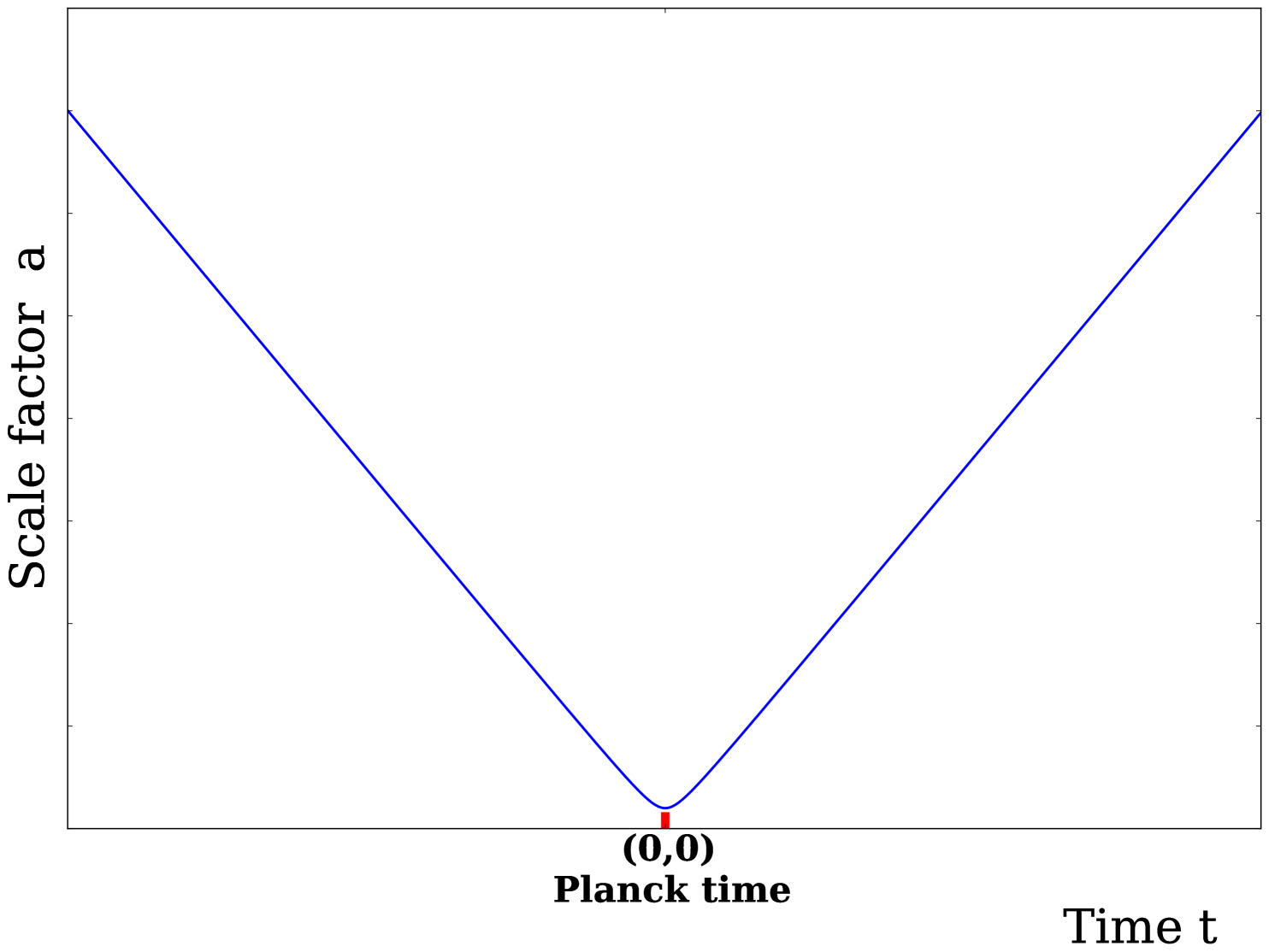
Figure 1: The variation of scale factor with time. The smooth bounce occurs in between the coasting contraction and the coasting expansion phases.

Surprisingly, the field equations in the above case can be rewritten in a form similar to that of a FLRW model. When redefined to have appropriate dimensions, the variable $\beta$ would correspond to a scalar field that fills this universe. By separating the real and imaginary parts of them, we obtain

$$\frac{\dot{a}^{2}}{a^{2}}+\frac{c^{2}}{a^{2}}=\dot{\beta}^{2}+\frac{2c^{2}}{a^{2}}\sin^{2}\beta,$$ (25)

$$2\frac{\ddot{a}}{a}+\frac{\dot{a}^{2}}{a^{2}}+\frac{c^{2}}{a^{2}}=3\left(\dot{\beta}^{2}+\frac{2c^{2}}{3a^{2}}\sin^{2}\beta\right),$$ (26)

$$\ddot{\beta}+2\dot{\beta}\frac{\dot{a}}{a}=0,$$ (27)

and

$$2\dot{\beta}\frac{\dot{a}}{a}=\frac{c^{2}}{a^{2}}\sin 2\beta.$$ (28)

These equations are similar to equations (7) - (9) for a universe filled with a scalar field. We may get the solution to $\beta(t)$ from the above equations as

$$\dot{\beta}(t)=\frac{\pm c\;a_{0}}{a^{2}(t)}=\frac{\pm c\;\cos^{2}\beta}{a_{0}},$$ (29)

and

$$\beta(t)=\tan^{-1}(\frac{\pm ct}{a_{0}}),$$ (30)

Substituting these solutions for $\beta$ and $\dot{\beta}$ into equations (25) and (26), one can write

$$\frac{{\dot{a}}^{2}}{a^{2}}+\frac{c^{2}}{a^{2}}=\frac{2c^{2}}{a^{2}}-\frac{c^{2}a^{2}_{0}}{a^{4}}$$ (31)

$$2\frac{\ddot{a}}{a}+\frac{\dot{a}^{2}}{a^{2}}+\frac{c^{2}}{a^{2}}=\frac{2c^{2}}{a^{2}}+\frac{c^{2}a^{2}_{0}}{a^{4}},$$ (32)

We now note that these equations result also from the variation of an action in (2), with the form of $\Lambda$ slightly modified than that given in (10). Here we must use

$$\Lambda=c^{2}\left(\frac{C_{4}}{a^{4}}-\frac{C_{2}}{a^{2}}\right),$$ (33)

where $C_{2}=3c^{2}/4\pi G$ and $C_{4}=3c^{2}a_{0}^{2}/8\pi G$. Such a real action that leads to the same equations (31)-(32) corresponds to a closed ($k=+1$) FLRW model with total energy density and pressure given by

$${\rho}=\frac{3c^{2}}{8\pi G}\left(\frac{2}{a^{2}}-\frac{a^{2}_{0}}{a^{4}}\right),$$ (34)

$${p}={-\frac{c^{4}}{8\pi G}}\left(\frac{2}{a^{2}}+\frac{a^{2}_{0}}{a^{4}}\right)$$ (35)

respectively. This physical model with the same evolution $a(t)=\sqrt{a_{0}^{2}+c^{2}t^{2}}$ can be shown to be a viable one with several positive features when compared to other models. For $ct\gg a_{0}$, this model coincides with an eternal coasting cosmological model discussed in mvjkbj3 , for the special case of $k=+1$. It may also be noted that another special case of the eternal coasting model in mvjkbj3 (one with $k=0$) is examined in detail under the title of ‘$R_{h}=ct$ cosmological model’ melia1 ; melia2 ; melia3 .

The quantities in equations (34) and (35) correspond to a conserved total energy-momentum tensor. However, we may consider the energy corresponding to this to be made up of constituents, that may or may not be separately conserved. An obvious conserved constituent of the above energy density is a negative energy density $\rho_{-}$, given by

$$\rho_{-}=-\frac{3c^{2}}{8\pi G}\frac{a^{2}_{0}}{a^{4}}.$$ (36)

This has pressure, given by

$$p_{-}=-\frac{c^{4}}{8\pi G}\frac{a^{2}_{0}}{a^{4}}$$ (37)

so that $p_{-}=(1/3)\rho_{-}c^{2}$. This negative energy, which closely resembles that of the Casimir energy casimir , has its density significant (when compared with the remaining part) only near the bounce mvjthesis . Such a bounce is sometimes referred to as a ‘Tolman wormhole’ coule . Another feature of the present model in connection with this energy density is that the gravitational charge ${\rho}c^{2}+3{p}$ for the model is

$${\rho}c^{2}+3{p}=-\frac{3c^{4}}{4\pi G}\frac{{a_{0}}^{2}}{a^{4}}.$$ (38)

Since the negative energy density disappears very quickly for $ct\gg a_{0}$, also the gravitational charge vanishes for $a(t)\gg a_{0}$. This leads to the coasting evolution for the very early/late epochs.

It was pointed out in mvjkbj1 ; mvjkbj2 ; mvjkbj3 ; mvjmnras that the remaining (conserved) part of the total density in (34) (that varies as $a^{-2}$) can be considered to be made up of ordinary matter (with equation of state $p_{m}=0$ or $p_{m}=\rho_{m}/3$) and a repulsive dark energy (with equation of state $p_{\Lambda}=-\rho_{\Lambda}c^{2}$). This can happen if there is creation of matter at the expense of the (decaying) dark energy. In the present epoch of the universe, the rate of creation of matter need only to be very small, so that it will hardly be observable.

Cosmological observations suggest that at the present epoch, densities of matter and dark energy have nearly the same magnitude. If this feature is true only for the present universe, such a near equality at the present epoch owes an explanation and this is referred to as the ‘coincidence problem’. It is easy to see that unless the dark energy density and the matter density vary in the same manner, there will appear a coincidence problem. We see that in the present model, no coincidence problem appears since one has both components varying as $a^{-2}$.

It may also be noted that this model is devoid of the so-called synchronicity problem kirshner . This is related to the value of the combination of physical quantities $H_{0}$, the present value of the Hubble constant and $t_{0}$, the age of the universe, estimated using direct methods. The observed value of the combination $H_{0}t_{0}$ is very close to unity, which is another coincidence since it could not have occurred at any other epoch in the universe. In the present model, this is however not a coincidence; this is true for all times and is a prediction of the model. Here it must be true at all epochs except during the initial bounce.

In addition to the absence of coincidence and synchronicity problems, the model is devoid of all problems discussed in Friedmann cosmology in the 1980s and 90s, such as the flatness, horizon, size and monopole problems. The present cosmological model agrees well with several cosmological observations, as discussed extensively in the literature mvjapj1 ; mvjapj2 ; melia1 ; melia2 ; melia3 ; mvjmnras .

4 Quantisation of the model

In order to quantise this model, let us start from the Lagrangian in $I_{G}$, the gravitational action, for a universe described by RW metric with real scale factor $a$. This Lagrangian may be written as

$$L_{G}=\frac{3\pi}{4G}c^{4}N\;{{a}^{3}}\left[\frac{1}{N^{2}c^{2}}\left(\frac{\dot{{a}}}{{a}}\right)^{2}-\frac{1}{{{a}^{2}}}\right],$$ (39)

omitting the negative sign. We note that $\dot{N}$ does not appear in this expression and hence the momentum conjugate to $N$, denoted by $\pi_{N}$, vanishes. The conjugate momentum to ${a}$ is

$$\pi_{{a}}=\frac{\partial L_{G}}{\partial\dot{{a}}}=\frac{3\pi}{2G}\frac{c^{2}}{N}{a}\dot{{a}}.$$ (40)

The canonical Hamiltonian is then

$${H_{c}}=N\left(\frac{3\pi c^{4}}{4G}{a}+\frac{G}{3\pi c^{2}}\frac{\pi_{{a}}^{2}}{{a}}\right)\equiv NH.$$ (41)

Since $\pi_{N}$ vanishes for all times, its time derivative, given by the Poisson bracket, also vanishes. That is,

$$\dot{\pi}_{N}=\{H_{c},\pi_{N}\}=\frac{\delta H_{c}}{\delta N}=0.$$ (42)

This leads to $H=0$, where $H$ is defined by (41). Such a classical constraint equation can be seen to be the consequence of time-reparametrisation invariance. In other words, $H=0$ ensures that using $dt^{\prime}=Ndt$ will not affect the equation of motion. Also, this allows us to choose some convenient gauge for $N$. Note that we have already chosen $N=1$ in the above sections. However, in the following discussion, we do not intend to set any such gauge for $N$.

The quantum theory of this model can now be formulated with ${a}$ as the field variable. The first step in quantising the classical model is to consider all observables, such as ${a}$, $\pi_{a}$, etc., as operators. The usual approach is to write the Wheeler-De Witt (WD) equation, given in Eq. (1), to take account of the classical constraint relation $H=0$. This is considered to be the wave equation for the universe, defined in a minisuperspace with only one coordinate ${a}$. However, here an operator-ordering ambiguity arises while replacing $\pi_{a}^{2}/{a}$ with differential operators. The usual approach is to adopt a factor-ordering parametrised by a constant $r$ kolbturner , such that

$$\pi_{a}^{2}\rightarrow-\hbar^{2}{a}^{-r}\left(\frac{\partial}{\partial{a}}{a}^{r}\frac{\partial}{\partial{a}}\right).$$ (43)

Various choices for the value of $r$ are made, hoping that its value will not significantly affect semiclassical calculations. Instead of pursuing this approach, in the present work, we adopt the well-known operator method to address the quantisation of the model. Here, one assumes ${a}$ and $\pi_{a}$ as operators that obey the fundamental commutation relation

$$[{a},\pi_{a}]=i\hbar.$$ (44)

In addition, let us postulate a commutation and an anticommutation relation between ${\pi_{a}^{2}}/{{a}}$ and ${a}$ as

$$\left[\frac{\pi_{a}^{2}}{{a}},{a}\right]=0.$$ (45)

and

$$\left\{\frac{\pi_{a}^{2}}{{a}},{a}\right\}=2\pi_{a}^{2},$$ (46)

respectively. This is useful in avoiding any operator-ordering ambiguity and helps circumventing arbitrary steps as in (43). Using Eq. (45), one can see that also ${a}$ and $H$ are commuting observables. i.e.,

$$[{{a}},H]=0.$$ (47)

The result that ${a}$ and $H$ commute does not lead to any conceptual problems; it only endorses the fact that the universe can have simultaneous eigenstates of ${a}$ and $H$. With this additional input, we define two new operators,

$$C=\frac{1}{\sqrt{\hbar c}}\left(\sqrt{\frac{3\pi c^{4}}{4G}}{a}+i\sqrt{\frac{G}{3\pi c^{2}}}\pi_{a}\right),$$ (48)

and

$$C^{\dagger}=\frac{1}{\sqrt{\hbar c}}\left(\sqrt{\frac{3\pi c^{4}}{4G}}{a}-i\sqrt{\frac{G}{3\pi c^{2}}}\pi_{a}\right).$$ (49)

We may now obtain the relation

$$C^{\dagger}C=\frac{1}{\hbar c}\left(\frac{3\pi c^{4}}{4G}{a}^{2}+\frac{G}{3\pi c^{2}}\pi_{a}^{2}-\frac{\hbar c}{2}\right).$$ (50)

Using the definition (41) for $H$ and the relations (45) and (46), one can write this expression as

$$C^{\dagger}C=\frac{1}{\hbar c}\left({a}H-\frac{\hbar c}{2}\right).$$ (51)

It may also be noted that

$$[{a},C^{\dagger}C]=0,\qquad[H,C^{\dagger}C]=0,\qquad[C,C^{\dagger}]=1,$$ (52)

and

$${a}H={\hbar c}\left(C^{\dagger}C+\frac{1}{2}\right).$$ (53)

$C^{\dagger}C$ can now be considered as a number operator, with

$$C^{\dagger}C\ket{n}=n\ket{n},$$ (54)

so that

$${a}H\ket{n}={\hbar c}\left(n+\frac{1}{2}\right)\ket{n}.$$ (55)

With the help of the commutation relations (44), (45), (46), (47) and (52), one can write

$${a}H(C\ket{n})={\hbar c}\left[(n-1)+\frac{1}{2}\right](C\ket{n}),$$ (56)

showing that $C$ is a lowering operator. Similarly,

$${a}H(C^{\dagger}\ket{n})={\hbar c}\left[(n+1)+\frac{1}{2}\right](C^{\dagger}\ket{n}).$$ (57)

showing that $C^{\dagger}$ is a raising operator. The ground state of the universe, with $n=0$, may then obey

$$C\ket{0}=0.$$ (58)

We can now write a differential equation that corresponds to this equation, without any operator-ordering ambiguity. This is as in the case of harmonic oscillator, but in terms of the minisuperspace coordinate ${a}$. The resulting differential equation, with $\braket{{a}}{{0}}\equiv\Psi_{0}({a})$, is

$$\frac{d\Psi_{0}({a})}{d{a}}+\frac{3\pi c^{3}}{2G\hbar}\;{a}\;\Psi_{0}({a})=0,$$ (59)

whose solution is

$$\Psi_{0}({a})=\exp\left(-\frac{{a}^{2}}{2\lambda^{2}}\right),$$ (60)

where $\lambda^{2}\equiv\frac{2G\hbar}{3\pi c^{3}}$. This solution is similar to that of the ground state harmonic oscillator. One can also see that this is the solution for an eigenvalue equation,

$${a}H\ket{0}=\frac{\hbar c}{2}\ket{0},$$ (61)

with ${\hbar c}/{2}$ as the eigenvalue. Then we can write the wave equation for the universe in the form

$${a}H\Psi_{0}({a})=\frac{\hbar c}{2}\Psi_{0}({a}).$$ (62)

Note that this equation is different from the WD equation (1), which is based on $H=0$. In fact, the zero energy condition $H=0$ is classical and one need not expect this to be exactly satisfied in a quantum theory too. In addition, the above equation does not contain time as a parameter and hence it is time-reparametrisation invariant, just as the WD equation. We claim that (62) is a more appropriate wave equation for the universe than the latter.

It may be noted that (62) rectifies a similar equation used in mvjkbj1 ; mvjkbj2 . In this reference, we anticipated the presence of a zero-point energy $\epsilon_{0}$, in a somewhat arbitrary manner. But in that case, we could not get an exact solution for the universe and hence no exact classical-quantum correspondence. In this paper we have shown, using the operator method, that the quantum ground state of the present model can be described by an exact solution of the problem, which is fit for the universe.

In the next section, we shall see that the results obtained above for the complex universe, based on the operator method, has exact classical-quantum correspondence.

5 Classical-quantum correspondence

We have obtained the ground ($n=0$) state of the universe as described by a Gaussian wave function, and now its correspondence with the classical solution needs to be verified. One expects that at least for large values of $a$, the wave function would correspond with the classical world. The usual approach to this is to check whether the probability distribution obtained from the wave function exactly peaks over a classical trajectory. However, it may be noted that here we have only one state for the universe and even the definition of probability in this context is quite vague. An alternative approach is to obtain the quantum trajectories of the given wave function and to check whether the trajectories agree with the classical ones, at least in the limiting case. We have seen in mvjgrco that the coasting evolution of the universe that starts from a singularity will have exact classical-quantum correspondence when checked in this manner. We show, using the MdBB complex trajectory formulation of quantum mechanics, that in the present case of complex cosmology too, there is exact correspondence between the quantum and classical description of the universe, throughout its history of evolution.

To demonstrate this, we make use of the equation of motion used in the trajectory approaches, given by

$$\pi_{{a}}=\frac{\partial S}{\partial{a}},$$ (63)

where $S$ is the action. In the MdBB approach, where the wave function is identified to be of the form $\Psi({a})=e^{iS({a})/\hbar}$ mvjqm1 , the action $S$ may be found to be

$$S=i\hbar\frac{{a}^{2}}{2{\lambda}^{2}}.$$ (64)

Since in general $S$ is a complex function, the momentum computed using (63) and also the trajectories may be complex. In the present case, the trajectories are obtainable from

$$\pi_{a}=\frac{\partial L_{G}}{\partial a}=\frac{3\pi}{2G}c^{2}a\dot{a}$$ (65)

Henceforth, we shall denote the complex trajectories as $\tilde{a}(t)$. Using (63), one obtains

$$\dot{\tilde{a}}=icN.$$ (66)

On integrating, we get

$$\tilde{a}=a_{0}+icNt.$$ (67)

Retaining the original negative sign in Eq. (39) (instead of omitting it) would be equivalent to writing $-N$ in place of $N$ in $L_{G}$. In that case, we get the above result as $\tilde{a}=a_{0}-icNt$. In the gauge $N=+1$, this is the same as the solution for ${\tilde{a}}$ in (23), which is the desired result. Thus the trajectories corresponding to the ground state of the quantum universe is precisely the same as that in the classical case and we have exact quantum-classical correspondence.

6 Discussion

Einstein considered the left hand side of his equation as nice and geometrical, while according to him the right hand side, which contains the energy-momentum tensor, is somewhat less compelling seancarroll . He is said to have even fancied that also $T_{\mu\nu}$ somehow followed from geometry. To our knowledge, there were no such attempts to address this possibility even for specific instances, other than that in the previous work mvjkbj1 ; mvjkbj2 . Here we showed that formulating a theory of gravity based solely on the gravitational action $I_{G}$, which contains only geometric terms, is possible at least in the case of cosmology. Analytic continuation of the Lagrangian function in $I_{G}$ to the complex plane of $\alpha(t)$, where the scale factor $a(t)=Ae^{\alpha(t)}$ in the $k=+1$ RW metric, results in the same field equations as in a closed FLRW universe with homogeneous and isotropic distribution of a new scalar field $\beta(t)$. Solving the Einstein equation in this case gives a bouncing and eternal coasting cosmological model. This model is shown to follow also from the action for a closed universe with homogeneous and isotropic distribution of energy/matter, with density varying as $a^{-2}$ and an additional negative energy density that varies as $a^{-4}$. The latter energy density is significant only near the bounce. This was shown to be a viable alternative to the $\Lambda$-CDM model in explaining the evolution of the background spacetime, while not exhibiting any of the conceptual problems that plague the $\Lambda$-CDM model. We developed a quantum theory for the complex model using an approach different from that of the Wheeler-DeWitt equation. While resorting to the operator method of canonical quantisation based on the fundamental commutation relations, it helped to circumvent the operator ordering ambiguity in the WD equation. Using this approach, we obtained a quantum wave equation for the universe, which is a modified WD equation. We find that the exact solution of this equation is an acceptable wave function for the universe. Most notably, we have shown that the solution of the present quantum wave equation corresponds to the classical solution in all respects, as per the MdBB trajectory formulation of quantum mechanics.

7 Acknowledgements

I wish to thank Professors K. Babu Joseph and K. P. Satheesh for enlightening discussions.

8 Declarations

Funding There was no funding for this work from any source.

Conflicts of interest/Competing interests The author declares no conflict of interests.

Availability of data and material The work does not use any data or material directly.

Code availability The work does not rely on any codes.

9 References

References

- (1) Susskind, L.: Dear qubitzers, gr= qm. arXiv:1708.03040v1 [hep-th] (2017)
- (2) John, M.V., Babu Joseph, K.: A modified Ozer-Taha type cosmological model. Phys. Lett. B 387, 466 arXiv:gr-qc/0312040v1 (1996)
- (3) John, M.V., Babu Joseph, K.: A low matter density decaying vacuum cosmology from a complex metric. Class. Quantum Grav. 14, 1115 arXiv:gr-qc/0007052 (1997)
- (4) John, M.V., Babu Joseph K.: Generalized Chen-Wu type cosmological model. Phys. Rev. D 61, 08730 arXiv:gr-qc/9912069 (2000)
- (5) John, M.V.: Cosmographic evaluation of the deceleration parameter using type Ia supernova data. Astrophys. J. 614, 1 arXiv:astro-ph/0406444 (2004)
- (6) John, M.V.: Cosmography, decelerating past, and cosmological models: learning the Bayesian way. Astrophys. J. 630, 667 arXiv:astro-ph/0506284 (2005)
- (7) Melia, F.: The cosmic horizon MNRAS 382, 1917 arXiv:0711.4181 (2007)
- (8) Melia, F., Shevchuk, A.: The universe MNRAS 419, 2579 arXiv:1109.5189 (2012)
- (9) Yennapureddy, M.K., Melia, F.: A comparison of the and CDM cosmologies based on the observed halo mass function Eur. Phys. J. C. 79, 571 arXiv:1907.00897 (2019)
- (10) John, M.V.: and the eternal coasting cosmological model. MNRAS 484, L35 arXiv:1902.05088 (2019)
- (11) Halliwell, J.J.: Introductory lectures on quantum cosmology Proc. Jerusalem Winter School on Quantum Cosmology ed. T. Piran et. al. World Scientific, Singapore, (1991)
- (12) John, M.V.: Exact classical correspondence in quantum cosmology. Grav. Cosmol. 21, 208 arXiv:1405.7957 (2015)
- (13) de Broglie, L.: Ph.D. Thesis. University of Paris, (1924); J. Phys. Rad., 6e serie, t. 8, 225 (1927)
- (14) Bohm, D.: A Suggested Interpretation of the Quantum Theory in Terms of ”Hidden” Variables. Phys. Rev. 85: 166 (1952)
- (15) John, M.V.: Modified de Broglie-Bohm approach to quantum mechanics. Found. Phys. Lett. 15, 329 arXiv:quant-ph/0109093 (2002)
- (16) John, M.V.: Probability and complex quantum trajectories. Ann. Phys. 324, 220 arXiv:0809.5101 (2009)
- (17) John, M.V.: Probability and complex quantum trajectories: Finding the missing links. Ann. Phys. 325, 2132 arXiv:1007.3838 (2010)
- (18) John, M.V., Mathew, K.: Coherent states and modified de Broglie-Bohm complex quantum trajectories. Found. Phys. 43, 859 arXiv:1104.3197 (2013)
- (19) Mathew, K., John, M.V.: Tunneling in energy eigenstates and complex quantum trajectories. Quantum Studies: Mathematical and Foundational 2, 403 arXiv:1512.05854 (2015)
- (20) Mathew, K., John, M.V.: Interfering quantum trajectories without which-way information. Found. Phys. 47, 873 arXiv:1806.00603 (2017)
- (21) Landau, L.D., Lifshitz, E.M.: Classical Theory of Fields. Pergamon, Oxford (1975)
- (22) Weinberg, S.: Gravitation and Cosmology Wiley, New York (1972)
- (23) Kolb, E.W., Turner, M.S.: The Early Universe. Addison-Wesley, Redwood City (1990)
- (24) Casimir, H.B.G.: On the attraction between two perfectly conducting plates. Proc. Kon. Ned. Akad. Wet. B. 51, 793 (1948)
- (25) John, M.V.: Studies on a New Cosmological Model from a Complex Metric. Ph.D. Thesis, Cochin University of Science and Technology, Kochi arXiv:gr-qc/0007053 (1999)
- (26) Coule, D.H.: Wormhole or bounce? Class. Quantum Grav. 10, L25 (1993)
- (27) Avelino, A., Kirshner, R.P.: The dimensionless age of the Universe: a riddle for our time. Astrophys. J 828, 35 arXiv:1607.00002 (2016)
- (28) Carroll, S.M.: Lecture Notes on General Relativity gr-qc/9712019 (1997)