Abstract

In this paper, the versions of quantum electrodynamics (QED) with spinors in fermion equations are briefly examined. In the new variants of the theory, the concept of vacuum polarization is unnecessary. The new content of fermion vacuum (without the Dirac sea) in the examined versions of QED leads to new physical consequences, part of which can be tested experimentally in the future.

Keywords: Quantum electrodynamics; bispinor and spinor functions; fermion vacuum; vacuum polarization; vacuum creation of pairs.

PACS numbers: 03.65.-w, 04.20.-q

1 Introduction

In the standard quantum electrodynamics (QED), the Dirac equation with the bispinor wave function is used to describe fermion states [1]. The Dirac equation has solutions with positive and negative energies. As a rule, the physical vacuum of the Dirac equation is described in terms of fully occupied states with negative energy (the Dirac sea).

In the Dirac vacuum, virtual creation and annihilation of electron-positron pairs is assumed. It is supposed that any electrical charge is surrounded by a cloud of virtual electron-positron pairs. It leads to decrease in initial charge, to reduce the effective Coulomb potential and to influence on the observed physical effects. This phenomenon is called vacuum polarization.

At electron scattering in the external electromagnetic field, the Feynman diagram, Fig.1, is considered for a manifestation of vacuum polarization in the lowest-order of the perturbation theory.

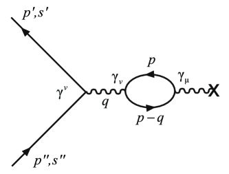
Figure 1: The Feynman diagram for vacuum polarization in the standard QED.

The accounting of the diagram, Fig. 1, contributes to the Lamb shift of the atomic levels. For hydrogen atom, this contribution to the level shift of $2S_{1/2}-2P_{1/2}$ is 27MHz.

The motion of fermions in the quantum theory can be described by equations with spinor functions. We will consider the two versions: the Foldy-Wouthuysen (FW) representation [2] and the representation with Klein-Gordon (KG)-type equation for fermions [3]. For these representations, we developed the formalisms of quantum electrodynamics (QED) ${}_{FW\,}$, (QED)${}_{KG\,}$ and calculated some physical effects [4], [5].

In the lowest order of the perturbation theory, the Coulomb cross-sections of an electron scattering, the scattering of an electron on a proton, the Compton effect, annihilation of an electron-positron pair are calculated. The self-energy of an electron, the anomalous magnetic moment of an electron, the Lamb shift of atomic energy levels are also calculated. The final results completely agree with the appropriate results in the standard QED with Dirac equation [4], [5].

The following is new in (QED) ${}_{FW\,}$ and (QED) _KG:

• The equation for electrons does not relate to the equation for positrons. These equations differ from each other by the signs of electrical charges and by the signs in front of the mass terms.

• In each of the equations, there is no relationship between the solutions with positive and negative energies.

• The content of the physical fermion vacuum varies.

The existence of the sea of solutions with negative energy (the Dirac sea), the processes of virtual creation and annihilation of electron-positron pairs, the concept of vacuum polarization seem to be excessive. The new content of the physical fermion vacuum leads to new physical effects.

Section 2 presents a brief review of the (QED) ${}_{FW\,}$ and (QED) _KG. In Secs. 3 and 4 we discuss the (QED) _FW and (QED) ${}_{KG\,}$ physical fermion vacuum and possible new physical effects. In the conclusion, we formulate the main conclusions of the paper.

In what follows, we use the system of units of $\hslash=c=1$ and the Minkowski space-time signature

$$g_{\alpha\beta}=\mbox{diag}\left\{{1,-1,-1,-1}\right\}.$$

2 The formalism of QED with spinor equations for fermions

The Dirac equation for an electron with mass $m$ interacting with the electromagnetic field can be written as

$$p^{0}\psi_{D}=H_{D}\psi_{D}=\left({{\bm{\alpha}}\left({{\rm{\bf p}}-e{\rm{\bf A}}}\right)+\beta m+eA^{0}}\right)\psi_{D},$$ (1)

where $H_{D}$ is the Dirac Hamiltonian, $p^{0}=i\left({\partial\mathord{\left/{\vphantom{\partial{\partial t}}}\right.\kern-1.2pt}{\partial t}}\right),\,\,{\rm{\bf p}}=-i\vec{{\nabla}}$; $A^{0}\left({{\rm{\bf r}},t}\right),\,\,{\rm{\bf A}}^{i}\left({{\rm{\bf r}},t}\right)$ are electromagnetic potentials; $\alpha^{k},\,\beta$ are four-dimensional Dirac matrixes; $k=1,2,3$.

The bispinor $\psi_{D}$ has the form

$$\psi_{D}=\left({{\begin{array}[]{*{20}c}{\varphi\left({{\rm{\bf x}},t}\right)U_{S}\hfill}\\ {\chi\left({{\rm{\bf x}},t}\right)U_{S}\hfill}\\ \end{array}}}\right).$$ (2)

The following equation can be used for description of positrons:

$$p^{0}\psi_{D}^{C}=\left({{\bm{\alpha}}\left({{\rm{\bf p}}+e{\rm{\bf A}}}\right)-\beta m-eA^{0}}\right)\psi_{D}^{C}.$$ (3)

Here $\psi_{D}^{C}=\beta\Sigma_{2}\psi_{D}^{*}$, $\Sigma_{2}=\left({{\begin{array}[]{*{20}c}{\sigma_{2}\,\,\,\ 0\hfill}\\ {0\,\,\,\ \sigma_{2}\hfill}\\ \end{array}}}\right)$, $\psi_{D}^{*}$ is complex conjugate bispinor.

Equation (3) differs from Eq. (1) by the signs of charge and mass.

In the free case (without interaction), the Dirac equations (1) and (3) have the following normalized solutions with positive and negative energies:

$$\begin{array}[]{l}\psi_{D}^{\left(+\right)}\left({{\rm{\bf x}},t;+m}\right)=\sqrt{\dfrac{E+m}{2E}}\left({\begin{array}[]{l}\,\,\,\,\,\,\,\,U_{S}\\[10.0pt] \dfrac{{\rm{\bm{\sigma}\bf p}}}{E+m}U_{S}\\[15.0pt] \end{array}}\right)e^{-iEt+i{\rm{\bf px}}},\\ \psi_{D}^{\left(-\right)}\left({{\rm{\bf x}},t;+m}\right)=\sqrt{\dfrac{E+m}{2E}}\left({\begin{array}[]{l}\dfrac{{\rm{\bm{\sigma}\bf p}}}{E+m}U_{S}\\[10.0pt] \,\,\,\,\,\,\,\,U_{S}\\ \end{array}}\right)e^{iEt-i{\rm{\bf px}}}.\\ \end{array}$$ (4)

$$\begin{array}[]{l}\psi_{D}^{C\,\,\left(+\right)}\left({{\rm{\bf x}},t;-m}\right)=\sqrt{\dfrac{E-m}{2E}}\left({\begin{array}[]{l}\,\,\,\,\,\,\,\,U_{S}^{C}\\[10.0pt] \dfrac{{\rm{\bm{\sigma}\bf p}}}{E-m}U_{S}^{C}\\[15.0pt] \end{array}}\right)e^{-iEt+i{\rm{\bf px}}},\\ \psi_{D}^{C\,\,\left(-\right)}\left({{\rm{\bf x}},t;-m}\right)=\sqrt{\dfrac{E-m}{2E}}\left({\begin{array}[]{l}\dfrac{{\rm{\bm{\sigma}\bf p}}}{E-m}U_{S}^{C}\\ \,\,\,\,\,\,\,\,U_{S}^{C}\\[10.0pt] \end{array}}\right)e^{iEt-i{\rm{\bf px}}}.\\ \end{array}$$ (5)

In Eqs. (2) – (5), $E=\sqrt{m^{2}+{\rm{\bf p}}^{2}}$; $\sigma^{k}$ are two-dimensional Pauli matrixes; $U_{S}^{C}=\sigma^{2}U_{S}$ are normalized Pauli spinors.

Solutions (4) and (5) were obtained by using matrices $\alpha^{k},\,\beta$ in the Dirac-Pauli representation. The similar solutions can be obtained with Dirac matrixes in the spinor representation widely used in the Standard Model. The QED with spinor equations for fermions and with the spinor representation of Dirac matrixes is presented in paper [6] - (QED) ${}_{FW\,}$ and in Ref. [7] - (QED) _KG. The final physical results in Refs. [6] and [7] coincide with the results in standard QED and with the results in Refs. [4] and [5] by using matrixes $\alpha^{k},\,\beta$ in the Dirac-Pauli representation.

2.1 QED in Foldy-Wouthuysen representation (QED) _FW

The Dirac equation in the FW representation can be obtained as a power series expansion in the electromagnetic coupling constant by using a number of unitary transformations $U_{FW}=\left({1+\delta_{1}+\delta_{2}+\delta_{3}+...}\right)U_{0}$ [4].

As the results, we obtain the following equations:

$$\begin{array}[]{l}p^{0}\psi_{FW}=H_{FW}\psi_{FW}=\left({\beta E+eK_{1}\left({+m,A^{\mu}}\right)+e^{2}K_{2}\left({+m,A^{\mu},A^{\nu}}\right)+}\right.\\[10.0pt] \left.{+e^{3}K_{3}\left({+m,A^{\mu},A^{\nu},A^{\gamma}}\right)+...}\right)\psi_{FW}.\end{array}$$ (6)

$$\begin{array}[]{l}p^{0}\psi_{FW}^{C}=H_{FW}^{C}\psi_{FW}^{C}=\left({\beta E-eK_{1}\left({-m,A^{\mu}}\right)+e^{2}K_{2}\left({-m,A^{\mu},A^{\nu}}\right)-}\right.\\[10.0pt] \left.{-e^{3}K_{3}\left({-m,A^{\mu},A^{\nu},A^{\gamma}}\right)+...}\right)\psi_{FW}^{C}.\end{array}$$ (7)

In the free case, we have

$$p_{0}\psi_{FW}^{0}=\beta E\psi_{FW}^{0},$$ (8)

where for the positive energy of $p_{0}=E$

$$\psi_{FW}^{0\,\,\left(+\right)}\left({{\rm{\bf x}},t}\right)=\left({\begin{array}[]{l}U_{S}\\ \,0\\ \end{array}}\right)e^{-iEt+i{\rm{\bf px}}},$$ (9)

For the negative energy of $p_{0}=-E$, we have

$$\psi_{FW}^{0\,\,\left(-\right)}\left({{\rm{\bf x}},t}\right)=\left({\begin{array}[]{l}\,0\\ \,U_{S}\\ \end{array}}\right)e^{iEt-i{\rm{\bf px}}}.$$ (10)

In case of interaction, Hamiltonians $H_{FW},H_{FW}^{C}$ in (6) and (7) are diagonal relative to the mixing of the upper and lower components of bispinor $\psi_{FW}$. Each of Eqs. (6) and (7) actually includes two independent equations with spinor wave functions $\sim U_{S}$.

In the equations of the FW-representation, masses of particles and antiparticles have the opposite signs [4]. If we use solutions (6) with positive energy and mass $\left({+m}\right)$ for electrons, then for positrons, we should use solutions (7) with positive energy and mass $\left({-m}\right)$.

In Ref. [4], the formalism of quantum electrodynamics (QED) ${}_{FW\,}$ is developed and some of physical effects are calculated. The final calculation results coincide with the results in the standard QED.

In (QED) ${}_{FW\,}$, the concept of vacuum polarization is unnecessary.

2.2 QED with the spinor equation for fermions of Klein-Gordon type

The self-conjugated equations for electrons and positrons with spinor wave functions are obtained in Refs. [3] and [5]. These equations are given by

$$\begin{array}[]{l}\left[{\left({p^{0}-eA^{0}}\right)^{2}-m^{2}-\left({p^{0}-eA^{0}+m}\right)^{1/2}{\rm{\bm{\sigma}}}\left({{\rm{\bf p}}-e{\rm{\bf A}}}\right)}\times\right.\\[10.0pt] \left.{\times\dfrac{1}{p^{0}-eA^{0}+m}{\rm{\bm{\sigma}}}\left({{\rm{\bf p}}-e{\rm{\bf A}}}\right)\left({p^{0}-eA^{0}+m}\right)^{1/2}}\right]\Phi=0,\end{array}$$ (11)

$$\begin{array}[]{l}\left[{\left({p^{0}+eA^{0}}\right)^{2}-m^{2}-\left({p^{0}+eA^{0}-m}\right)^{1/2}{\rm{\bm{\sigma}}}\left({{\rm{\bf p}}+e{\rm{\bf A}}}\right)}\times\right.\\[10.0pt] \left.{\times\dfrac{1}{p^{0}+eA^{0}-m}{\rm{\bm{\sigma}}}\left({{\rm{\bf p}}+e{\rm{\bf A}}}\right)\left({p^{0}-eA^{0}-m}\right)^{1/2}}\right]\Phi^{C}=0.\\ \end{array}$$ (12)

In Eqs. (11) and (12), we can perform expansion in power of the charge $e$

$$\begin{array}[]{l}\left[{p_{0}^{2}-{\rm{\bf p}}^{2}-m^{2}\mp eV_{1}\left({\pm m,A^{\mu}}\right)-e^{2}V_{2}\left({\pm m,A^{\mu},A^{\nu}}\right)\mp}\right.\\[10.0pt] \left.{\mp e^{3}V_{3}\left({\pm m,A^{\mu},A^{\nu},A^{\gamma}}\right)-...}\right]\Phi\left({\pm m,{\rm{\bf x}},t}\right)=0.\end{array}$$ (13)

In (13), the upper signs before charge and mass correspond to Eq. (11) for electron, the lower signs correspond to Eq. (12) for positron. In Eqs. (11) and (13) $\Phi\left({+m,{\rm{\bf x}},t}\right)=\Phi$, in Eqs. (12) and (13) $\Phi\left({-m,{\rm{\bf x}},t}\right)=\Phi^{C}$.

The algorithm to determine the interaction operator of $V=\pm eV_{1}+e^{2}V_{2}\pm e^{3}V_{3}+...$ is given in Ref. [5].

In the free case, Eqs. (11) and (12) have the form of KG equations with spinor wave functions

$$\left({p_{0}^{2}-{\rm{\bf p}}^{2}-m^{2}}\right)\Phi_{0}\left({{\rm{\bf x}},t}\right)=0.$$ (14)

The orthonormal solutions $\Phi_{0}^{\left(\pm\right)}$ with positive and negative energies are given by

$$\Phi_{0}^{\left(\pm\right)}\left({{\rm{\bf x}},t}\right)=\frac{1}{\sqrt{2E}}e^{\mp iEt\pm i{\rm{\bf px}}}U_{S}.$$ (15)

In Ref. [5], the formalism of quantum electrodynamics (QED) ${}_{KG\,}$ is developed and some of physical effects are calculated. As well as in the representation (FW), the final computational results coincide with the results in the standard QED.

In (QED) ${}_{KG\,}$, the solutions with positive and negative energies of fermions in Eq. (13) are not connected with each other. In (QED) _KG equations, the masses of particles and antiparticles have different signs. In (QED) _KG, the content of physical vacuum varies and the concept of vacuum polarization is unnecessary.

3 Physical vacuum for fermions: the lack of vacuum polarization in QED with spinor equations for fermions

In the standard QED with the Dirac equation, the fermion vacuum represents the continuum of fully occupied states with negative energies (the Dirac sea, see Fig.2)

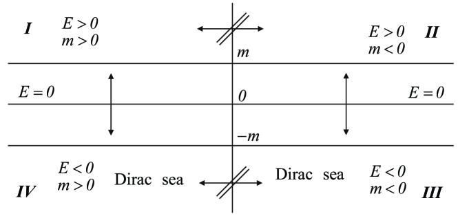
Figure 2: The physical vacuum of the Dirac equation.

In the standard QED, there exists the interaction of states with positive and negative energies. The solutions with different signs before the particle masses do not interact with each other. If we use quadrants I and IV of Fig. 2 with $m>0$, then the solutions with $m<0$ in quadrants II and III do not carry new physical information.

The holes in quadrant IV of Fig. 2 with $E<0$ represent the states of antiparticles in the standard QED. In theory, the possibility of spontaneous vacuum creation and annihilation of virtual particle-antiparticle pairs is admitted. As the result, the concept of vacuum polarization emerges. It is assumed that any charge is surrounded by a cloud of virtual particle-antiparticle pairs. It leads to efficient decrease in the value of the bare electrical charge that manifests itself in calculations of the Lamb shift of atomic energy levels.

Now, let us turn to the physical vacuum of the fermion equations with spinor functions (see Fig. 3).

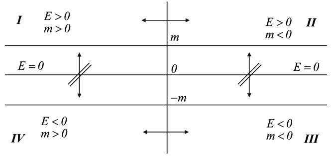
Figure 3: The physical vacuum of fermion equations with spinor functions.

Unlike the standard QED, there is no interaction between the states with positive and negative energies in the (QED) ${}_{FW\,}$ and (QED) ${}_{KG\,}$. In this connection, an introduction of the Dirac sea is unnecessary.

The physical fermion vacuum in (QED) ${}_{FW\,}$ and (QED) ${}_{KG\,}$, when using quadrants I, II, represents completely unoccupied states of particles with $E>0,m>0$ and completely unoccupied states of antiparticles with $E>0,m<0$. In equations of this theory, masses of particles and antiparticles should always have different signs.

While using quadrant I with $E>0,m>0$ for particles, the calculations of concrete physical effects in (QED) ${}_{FW\,}$ and (QED) ${}_{KG\,}$ are performed only with participation of intermediate (virtual) states with positive energy. For antiparticles of quadrant II with $E>0,m<0$, only virtual states with positive energy are also involved. In the theories under consideration, there is no need to take into account the process of creation and annihilation of virtual particle-antiparticle pairs. While using Eqs. (6), (7), (11) and (12) in (QED) ${}_{FW\,}$ and (QED )_KG, only the processes with real particles and antiparticles with opposite signs before their masses are taken into account. Only in this case, the interaction of the particles from the quadrant I with the antiparticles from the quadrant II is possible.

In Figs. 4 and 5, the Feynman diagrams in (QED) _FW, (QED) _KG, related to the self-energy function of a photon, and equivalent to the diagram in Fig. 1 in standard QED are presented in case of electron scattering in the external electromagnetic field.

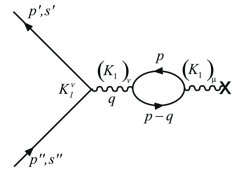
a)

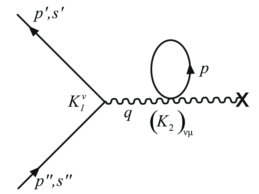
b)

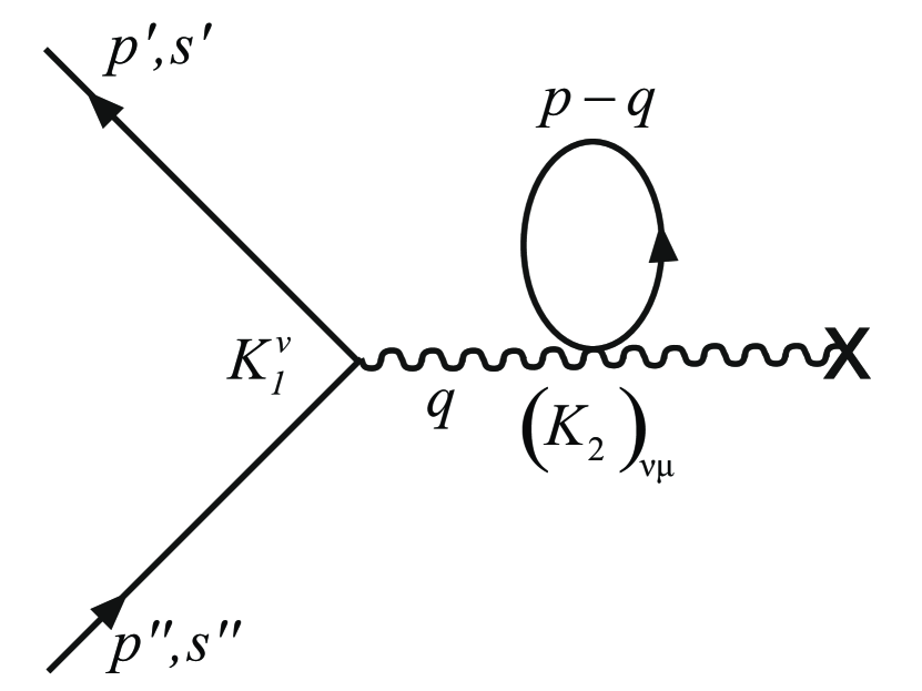
c)

Figure 4: The Feynman diagrams in (QED)_FW.

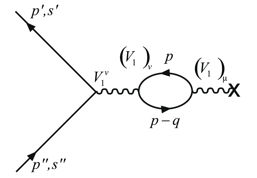
a)

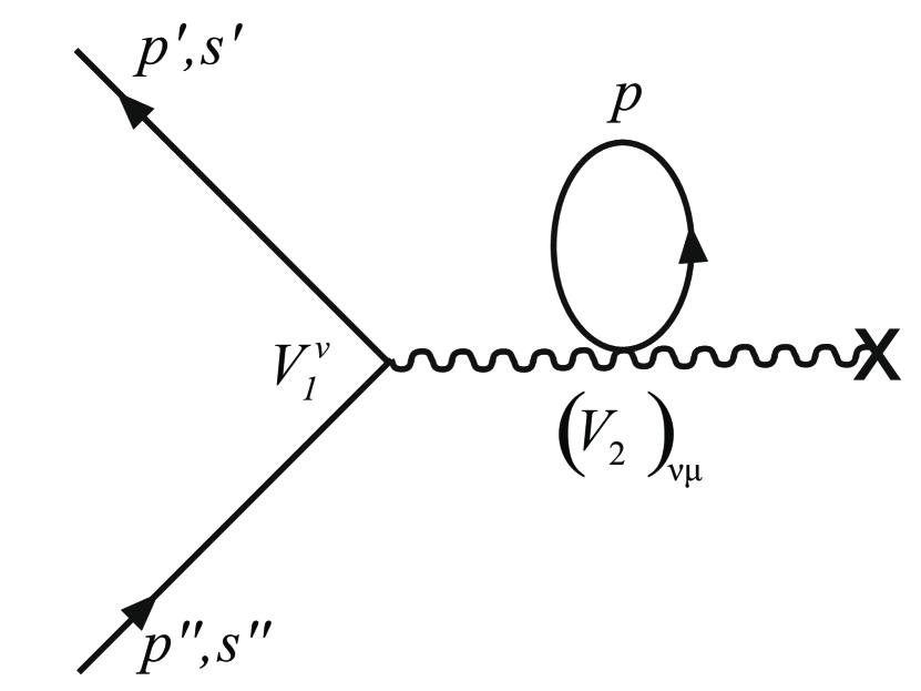
b)

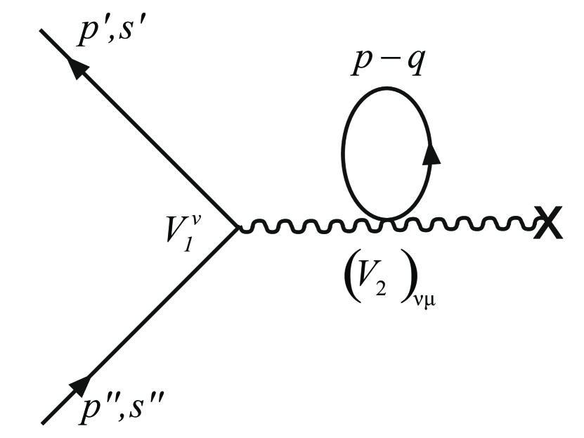
c)

Figure 5: The Feynman diagrams in (QED)_KG.

The final results of the computations of the diagram in Fig.1 in the standard QED coincide with the computational results of the diagrams in Fig. 4 in (QED) ${}_{FW\,}$ and the computational results of the diagrams in Fig. 5 in (QED) _KG.

However, while diagrams in Figs. 4(a) and 5(a) can be described in terms of creation and annihilation of virtual electron-positron pairs, diagrams in Figs. 4(b), 4(c) and 5(b), 5(c) cannot be interpreted in this way. Let us note again that the all physically observed effects for particles and antiparticles are described by using only the intermediate states with positive energy.

It follows from the above-mentioned that there are no processes of creation and annihilation of virtual fermion ”particle-antiparticle” pairs in (QED) ${}_{FW\,}$ and (QED) _KG. In these theories, the concept of vacuum polarization is unnecessary.

4 Discussion

The new state of the fermion vacuum in (QED)${}_{FW\,}$ and (QED)${}_{KG\,}$ leads to new physical consequences. Some of them can be tested experimentally in the future:

• In (QED) ${}_{FW\,}$ and (QED) _KG, there is no Zitterbevegung of fermion coordinates. This fact, associated with the absence of virtual interaction between the states of the fermions with positive and negative energies, was already mentioned in the first article of Foldy-Wouthuysen [2].

• For the same reasons in (QED) ${}_{FW\,}$ and (QED) _KG, there is no Klein paradox [8] (see App. A and Ref. [9]).

• In (QED) ${}_{FW\,}$ and (QED) _KG, there is no effect of vacuum creation of fermion particle-antiparticle pairs in strong electromagnetic fields. The Schwinger effect, i.e. vacuum creation of pairs in a strong homogeneous electrical field, is also absent [10].

• Because of absence of the Dirac sea in (QED) ${}_{FW\,}$ and (QED) _KG, the effect of vacuum creation of two electron-positron pairs is also absent at the achievement of the value of the nucleus charge of $Z=Z_{cr}\simeq 170$ for $1S_{1/2}$-state of the hydrogen-like atom [11]. In the theories under consideration, a minimal possible value of energy $E=0$ will be achieved for $1S_{1/2}$-state at $Z_{1S_{1/2}}\simeq 145$ already [11]. With the following increase in $Z$, the level $1S_{1/2}$ disappears. The next level of $2P_{1/2}$ disappears at $Z_{2P_{1/2}}\simeq 170$. The values of $Z_{1S_{1/2}},Z_{2P_{1/2}}$ etc. depend on the model of the finite size of an atomic nucleus [12].

• In quantum gravitational theories, similar to (QED) ${}_{FW\,}$ and (QED) _KG, there is no effect vacuum creation of fermion particle-antiparticle pairs. In this case, evaporation of black holes is possible only at the expense of vacuum creation of boson pairs.

• The analysis of the equations with spinor wave functions in the Coulomb repulsive field in (QED) ${}_{KG\,}$ has shown the availability of the impenetrable potential barrier in the effective potential with a radius proportional to the classical fermion radius and inversely proportional to the fermion energy (at $E\gg mc^{2})$ [3]. The existence of the impenetrable barrier does not contradict the results of the experiments in probing the internal structure of an electron and has no effect on the cross section of the Coulomb scattering of electrons in the lowest-order of the perturbation theory.

• In equations of (QED) _FW and (QED) _KG, masses of particles and antiparticles have the different signs [4, 5]. For the first time author shown this in 1989 (see Refs. [13] and [14]). Later, the other researchers came to the same conclusion (see, for example, Refs. [15] and [16]). In this paper, we do not establish linkage between different signs before masses of particles and antiparticles with problems of gravitation and antigravitation.

5 Conclusion

In versions of quantum electrodynamics with spinors in fermion equations, the concept of vacuum polarization is unnecessary.

The new content of the fermion vacuum (without the Dirac sea) leads to new physical consequences, part of which can be experimentally tested in the future.

Appendix A. The Foldy-Wouthuysen representation: the scattering on a step potential

In domain I, $E=\beta\sqrt{m^{2}+p^{2}}$.

In domain II, $E-eA^{0}=\beta\sqrt{m^{2}+q^{2}}$.

For the FW-representation, there is no relationship between the solutions of the FW equation with different signs of $\beta$. In compliance with the Figure, in domain I, $\beta=1,E>0$. Hence, $\beta=1,E-eA^{0}\geq 0$ in domain II as well. For imaginary $q$, $\left|q\right|^{2}\leq m^{2}$ should be fulfilled.

The Klein paradox is not available. The similar examination can also be performed for (QED) _KG.

References

- [1] P. A. M. Dirac, The Principles of Quantum Mechanics (Oxford University Press, 1930).
- [2] L. L. Foldy and S. A. Wouthuysen, Phys. Rev. 78, 29 (1950).
- [3] V. P. Neznamov and I. I. Safronov, J. Exp. Theor. Phys. 128, 672 (2019), arXiv: 1907.03579 (physics.gen-ph, hep-th).
- [4] V. P. Neznamov, Phys. Part. Nuclei 37, 86 (2006), arXiv: hep-th/0411050.
- [5] V. P. Neznamov and V. E. Shemarulin, Int. J. Mod. Phys. A. 36, 2150086 (2021), DOI: 10.1142/S0217751X2150086X.
- [6] V. P. Neznamov, Phys. Part. Nuclei 43, 36 (2012); arXiv: 1107.0693 (physics. gen-ph).
- [7] L. S. Holster, J. Math. Phys. 26, 1348 (1985).
- [8] O. Klein, Z. Phys. 53, 157 (1929).
- [9] Y. V. Kononets, Found. Phys. 40, 545 (2010).
- [10] J. Schwinger, Phys. Rev. 82, 664 (1951).
- [11] W. Pieper and W. Greiner, Z. Phys. 218, 327 (1969).
- [12] V. P. Neznamov and I. I. Safronov, Phys. Usp. 57, 189 (2014), arXiv: 1307.0209 (physics.atom-ph).
- [13] V. P. Neznamov, Voprosy Atomnoy Nauki i Tekhniki. Ser. Teoreticheskaya i Prikladnaya Fizika 1, 3 (1989) (in Russian).
- [14] V. P. Neznamov, Voprosy Atomnoy Nauki i Tekhniki. Ser. Teoreticheskaya i Prikladnaya Fizika 1-2, 4 (2004) (in Russian).
- [15] G-J. Ni, Rel. Grav. Cosmol. 1 (2004) 123-136, arXiv: 0308038v1 [physics. gen-ph]; G-J. Ni, S. Chen, S. Lou and J. Xu, arXiv: 1007.3051v1 [physics. gen-ph].
- [16] N. Debergh, J-P. Petit and G. D’Agostini, arXiv: 1809.05046v2 [quant-ph].