Coupled Helmholtz Equations : Chirped Solitary Waves

Abstract

We investigate the existence and stability properties of the chirped gray and anti-dark solitary waves within the framework of coupled cubic nonlinear Helmholtz equation in the presence of self steepening and self frequency shift. We show that for a particular combination of the self steepening and the self frequency shift, there is not only chirping but also chirp reversal. Specifically, the associated nontrivial phase has two intensity dependent terms, one varies as the reciprocal of the intensity while the other, which depends on non-Kerr nonlinearities, is directly proportional to the intensity. This causes chirp reversal across the solitary wave profile. A different combination of non-Kerr terms leads to chirping but no chirp reversal.The influence of nonparaxial parameter on physical quantities such as intensity, speed and pulse-width of the solitary waves is studied too. It is found that the speed of the solitary waves can be tuned by altering the nonparaxial parameter. Stable propagation of these nonparaxial solitary waves is achieved by an appropriate choice of parameters.

Coupled Helmholtz equations describe the evolution of broad multi-component self-trapped beams in Kerr-type nonlinear media along with spatial dispersion originating from the nonparaxial effect that becomes important, for example, in progressive miniaturization of optical devices where the optical wavelength is comparable to the beam width. To study the propagation of ultrashort optical pulses in the nonparaxial regime, it is necessary to include non-Kerr terms like the self steepening and the self frequency shift into the framework of coupled Helmholtz system. We present analytical chirped solitary wave solutions to the coupled Helmholtz equations incorporating the self steepening and the self frequency shift. The solutions comprise chirped gray, anti dark solitary waves depending upon the nature of the nonlinearities. The conditions on the model parameters for the existence of the derived chirped solitary structures have also been presented. For a particular combination of the self steepening and the self frequency shift parameters the associated nontrivial phase gives rise to chirp reversal across the solitary wave profiles. A different combination of non Kerr terms leads to chirping but no chirp reversal. The effect of the nonparaxial parameter on physical quantities like intensity, speed and pulse-width of the solitary waves is studied too. Numerical simulations have been performed which verify the stability of solitary wave solutions for the chosen parameters.

1 Introduction

In nonlinear optics, coupled nonlinear Schrödinger equation (NLSE) is the governing equation for pulse propagation in multi-mode optical fiber and also for coherent beam propagation in photo-refractive media [1]. Coupled NLSE gives rise to multi-component localized structures (vector solitons) that result from the balance between the dispersion and the self and the cross phase modulation in the case of pulse propagation and the balance between diffraction and locally induced refractive index changes in the case of beam propagation through a nonlinear optical medium [2]. The vector extension of the scalar NLSE to describe multicomponent pulse-beam evolution in the presence of Kerr nonlinearity was proposed by Manakov [3].

The derivation of NLSE stems from Maxwell’s equations by employing paraxial approximation or slowly varying envelope approximation which holds if the optical beams are (i) much broader than their carrier wavelength (ii) of sufficiently low intensity and (iii) propagating along (or at negligible angles with respect to) the reference axis. If all three conditions are not satisfied simultaneously, the beam is referred to as “non-paraxial” [4]. Interest on non paraxial beams has started attracting interest [5] after the pioneering work of Lax et al [6] who considered propagation of ultra-narrow beams i.e. where Condition (i) above no longer holds. On the other hand, the Helmholtz non-paraxiality i.e. when broad beams propagate at arbitrary angles with respect to the reference direction i.e. when only condition (iii) is relaxed, was considered in [4, 7, 8]. Exact analytical soliton solutions to scalar Helmholtz equation with focusing, defocusing Kerr nonlinearity, power law and polynomial nonlinearity as well as in anomalous and normal group velocity dispersion regimes are known [4, 9]. The formation and propagation of chirped elliptic and solitary waves in cubic-quintic nonlinear Helmholtz (NLH) system and the modulation instability has been studied in [10].

The Helmholtz-Manakov equation has been introduced for the first time in [11] for describing the evolution of broad multi-component self-trapped beams in Kerr-type media. Exact analytical bright-bright and bright-dark vector soliton solutions in the self-focusing Kerr media and dark-bright and dark-dark soliton solutions in the self-defocusing Kerr-media have been obtained. Scalar and vector nonlinear nonparaxial evolution equations are developed in [16] for propagation in two dimensions. Exact and approximate solutions to these equations are obtained and are shown to exhibit quasi-soliton behavior based on propagation and collision studies. The elliptic and the hyperbolic solitary wave solutions to the coupled NLH system are obtained in [17] and effect of non-paraxiality on speed, pulse-width and amplitude of various solutions are explored. Coupled nonparaxial (2+1) dimensional nonlinear Schrödinger equation has been considered in [18] and bright-bright, dark-dark and bright-dark soliton solutions are obtained. Modulation instability of the system of equations is studied too.

On the other hand, the study of the chirped solitons has attracted considerable interest in recent times. The important qualitative feature of chirping is its ability to compress and amplify solitary pulses in optical fiber which have important applications in optical fiber amplifiers/compressors and long-haul links [19, 20]. But these studies [21] have been restricted mainly to paraxial regime. In many of these works non-Kerr terms like the self-steepening and the self frequency shift have been considered as these are important in the study of propagation of ultrashort pulses [22]. This has motivated us to consider the coupled NLH system with non-Kerr terms like the self steepening and the self frequency shift. The inclusion of non Kerr terms may lead to important physical effects and therefore this is a topic well worth investigating.

Thus the main aim of this article is to show that the cubic coupled Helmholtz system with non Kerr nonlinearities admits chirped gray and anti-dark (depending upon the nature of nonlinearity) solitary waves, both of which show not only chirping but also chirp reversal for a particular combination of self steepening and self frequency shift. This is the novel physical effect emerging from the inclusion of non Kerr nonlinearity into the coupled Helmholtz system. Specifically, for a particular relation between the self steepening and the self frequency shift parameters, these solutions are characterized by nontrivial phase and have two intensity dependent chirping terms. One varies as the reciprocal of the intensity while the other, which depends on non-Kerr nonlinearities, is directly proportional to the intensity. As a result chirp reversal occurs across the wave profile. For a different relation between the non-Kerr terms, there exists only one intensity dependent term which is inversely proportional to the intensity, resulting in chirping but no chirp reversal. The influence of nonparaxial parameter on intensity, speed and pulse width of the solitary waves is studied too.

The article is organized as follows. In sec. II we elaborate on the theoretical model of the coupled NLH system with non-Kerr nonlinearity describing the propagation of the nonparaxial solitary waves and obtain the general expression for the phase (chirping) of the two components. Chirped solitary wave solutions are obtained in sec. III. The characteristic features of the exact solutions and their physical implications are studied too. The results of numerical simulations done to check the stability of the solitary waves are also presented. Finally, in Section IV, we summarize the results obtained in this article and indicate possible relevance of these results.

2 Theoretical model of the coupled Helmholtz syatem

The evolution of broad multicomponent self trapped beams in Kerr-type media without slowly varying envelope approximation is given by [11] the coupled equations

$$iq_{1z}+\kappa q_{1zz}+\frac{1}{2}q_{1tt}+(\bar{\sigma}_{1}|q_{1}|^{2}+\bar{\sigma}_{2}|q_{2}|^{2})q_{1}=0\,,$$ (1)

$$iq_{2z}+\kappa q_{2zz}+\frac{1}{2}q_{2tt}+(\bar{\sigma}_{1}|q_{1}|^{2}+\bar{\sigma}_{2}|q_{2}|^{2})q_{2}=0\,,$$ (2)

where $q_{j},j=1,2$ are the envelope fields of the first and the second components respectively, subscripts $z$ and $t$ represent the longitudinal and the transverse coordinates respectively.and $\kappa(>0)$ is the nonparaxial parameter. The second term in Eqns. (1) and (2) represents spatial dispersion originating from the nonparaxial effect with $\kappa(>0)$ being the nonparaxial parameter and the third term represents group velocity dispersion. $\bar{\sigma}_{i},i=1,2$ are the nonlinearity coefficients. For $\bar{\sigma_{1}}=\bar{\sigma_{2}}=\pm 1$, the above equations reduce to Helmholtz-Manakov system introduced in [11], with $+$ sign denoting a focusing and $-$ sign denoting a defocusing nonlinearity.
Helmholtz-Manakov system is appropriate for modelling the propagation and interaction of broad vector beams/pulses at arbitrary angles with respect to the reference direction (Helmholtz nonparaxiality) so long the width of the pulses are in the picosecond scale. As one increases the intensity of the incident light to produce shorter (femtosecond) pulses, non-Kerr nonlinear terms like self steepening and self frequency shift become important and need to be incorporated into the equations. Accordingly, in the presence of non Kerr terms Eqns. (1) and (2) get modified to

$$iq_{1z}+\kappa q_{1zz}+\frac{1}{2}q_{1tt}+(\bar{\sigma}_{1}|q_{1}|^{2}+\bar{\sigma}_{2}|q_{2}|^{2})q_{1}+i[a_{4}(|q_{1}|^{2}q_{1})_{t}+a_{5}q_{1}|q_{1}|^{2}_{t}]=0\,,$$ (3)

$$iq_{2z}+\kappa q_{2zz}+\frac{1}{2}q_{2tt}+(\bar{\sigma}_{1}|q_{1}|^{2}+\bar{\sigma}_{2}|q_{2}|^{2})q_{2}+i[a_{4}(|q_{2}|^{2}q_{2})_{t}+a_{5}q_{2}|q_{2}|^{2}_{t}]=0\,,$$ (4)

The term proportional to $a_{4}$ represents self steepening [12]. The latter produces a temporal pulse distortion leading to the development of an optical shock on the trailing edge of the pulse unless balanced by the dispersion [13]. This phenomenon is due to the intensity dependence of the group velocity that makes the peak of the pulse move slower than the peak [14]. The last term proportional to $a_{5}4$has its origin in the delayed Raman response [14] which forces the pulse to undergo a frequency shift known as self frequency shift [15].

To construct chirped periodic and solitary wave solutions of the coupled Eqns. (3) and (4), we consider the following traveling wave ansatz

$$q_{j}(z,t)=f_{j}(\xi)e^{i[\phi_{j}(\xi)-k_{j}z+\zeta_{j}]}\,,~{}~{}j=1,2$$ (5)

where $\xi=\beta(t-vz)$, $v=\frac{1}{u}$, $u$ being the group velocity of the wave packet, $k_{j},\zeta_{j},j=1,2$ are the wave numbers and real constants respectively. The chirp is given by

$$\delta\omega_{j}=-(\partial/\partial t)[\phi_{j}(\xi)-k_{j}z+\zeta_{j}]=-\beta\frac{d\phi_{j}}{d\xi},j=1,2\,.$$ (6)

Substituting the ansatz (5) into Eqns. (3) and (4), collecting the imaginary parts and integrating the resulting equations, we obtain

$$\phi_{1}^{\prime}(\xi)=\frac{c_{1}}{f_{1}^{2}}+\frac{a_{1}}{2a}-\frac{\beta(3a_{4}+2a_{5})f_{1}^{2}}{4a},~{}~{}~{}\phi_{2}^{\prime}(\xi)=\frac{c_{2}}{f_{2}^{2}}+\frac{a_{2}}{2a}-\frac{\beta(3a_{4}+2a_{5})f_{2}^{2}}{4a}\,,$$ (7)

where $c_{1}$ and $c_{2}$ are the integration constants while $a,a_{1},a_{2}$ are given by

$$a=\beta^{2}(\kappa v^{2}+1/2)>0\,,~{}~{}a_{1}=\beta v(1-2\kappa k_{1})\,,~{}~{}a_{2}=\beta v(1-2\kappa k_{2})\,.$$ (8)

Hence the chirping comes out to be

$$\delta\omega_{i}=-\beta\left(\frac{a_{i}}{2a}+\frac{c_{i}}{f_{i}^{2}}-\frac{\beta(3a_{4}+2a_{5})f_{i}^{2}}{4a}\right),~{}~{}i=1,2\,,$$ (9)

which depends on velocity $u$, wave numbers $k_{i},i=1,2$, nonparaxial parameter $\kappa$ and the intensities $f^{2}_{i},i=1,2$ of the chirped pulse. It is worth pointing out that the second term on the right hand side of Eqn. (9) is of the kinematic origin and is inversely proportional to the intensity of the solitary wave while the first term is a constant. The last term is directly proportional to the intensity of the resulting wave and leads to the chirping that is inverse to that coming from the second term. As a result, so long $3a_{4}+2a_{5}\neq 0$, one not only have chirping but also chirping reversal.

On substituting the ansatz (5) into Eqns. (3) and (4), collecting the real parts we arrive at the equations

$$f_{1}^{{}^{\prime\prime}}+d_{1}f_{1}+(\sigma_{1}f_{1}^{2}+\sigma_{2}f_{2}^{2})f_{1}+\beta_{1}f_{1}^{5}-\delta_{1}f_{1}^{3}=\frac{c_{1}^{2}}{f_{1}^{3}}\,,$$ (10)

and

$$f_{2}^{{}^{\prime\prime}}+d_{2}f_{2}+(\sigma_{1}f_{1}^{2}+\sigma_{2}f_{2}^{2})f_{2}+\beta_{1}f_{2}^{5}-\delta_{2}f_{2}^{3}=\frac{c_{2}^{2}}{f_{2}^{3}}\,,$$ (11)

where

$$d_{1}=\frac{a_{1}^{2}+4ab_{1}+2\beta c_{1}a(a_{4}+2a_{5})}{4a^{2}}\,,~{}~{}d_{2}=\frac{a_{2}^{2}+4ab_{2}+2\beta c_{2}a(a_{4}+2a_{5})}{4a^{2}}\,,$$

$$\sigma_{1,2}=\frac{\bar{\sigma}_{1,2}}{a}\,,~{}~{}\delta_{1}=\frac{\beta a_{4}a_{1}}{2a^{2}}\,,~{}~{}\delta_{2}=\frac{\beta a_{4}a_{2}}{2a^{2}}\,,~{}~{}b_{1}=k_{1}(1-\kappa k_{1})\,,~{}~{}b_{2}=k_{2}(1-\kappa k_{2})\,,$$

$$\beta_{1}=\frac{\beta^{2}(3a_{4}+2a_{5})(a_{4}-2a_{5})}{16a^{2}}\,.$$ (12)

We have been able to obtain the analytical solutions of the coupled Eqns. (10) and (11) in case $f_{2}$ and $f_{1}$ are proportional to each other, i.e. $f_{2}(\xi)=\alpha f_{1}(\xi)$, with $\alpha$ being a real number. This gives

$$\beta_{1}=0\,,~{}~{}d_{1}=d_{2}\,,~{}~{}c_{2}^{2}=\alpha^{4}c_{1}^{2}\,~{}~{}\delta_{1}=\alpha^{2}\delta_{2}\,.$$ (13)

Now $\beta_{1}=0$ can be satisfied for nonzero $a_{4},a_{5}$ if either (i) $a_{4}=2a_{5}\implies$ chirping with chirp reversal or (ii) $3a_{4}+2a_{5}=0\implies$ chirping but no chirp reversal. We shall focus on the case $a_{4}=2a_{5}$ and explicitly show the chirp reversal occurring in the phase of the constructed solitary wave solutions for focusing, defocusing and mixed nonlinearities.

The relations in (13) give the dependency of $\alpha$, integration constants $c_{1},c_{2}$ on the physical parameters as

$$\alpha^{2}=\frac{1-2\kappa k_{1}}{1-2\kappa k_{2}}\,,~{}~{}c_{1}=\frac{\beta(k_{2}-k_{1})(1-2\kappa k_{2})}{4aa_{4}}\,,\rm{when}~{}~{}c_{2}=-\alpha^{2}c_{1}\,,$$

$$c_{1}=\frac{\beta[\kappa(k_{1}+k_{2})-1](1-2\kappa k_{2})}{4aa_{4}\kappa},~{}\rm{when}~{}~{}c_{2}=\alpha^{2}c_{1}\,,$$ (14)

In what follows, we shall take $c_{1}=\frac{\beta(k_{2}-k_{1})(1-2\kappa k_{2})}{4aa_{4}}$, $\bar{\sigma_{1}}=\pm 1$ and $\bar{\sigma_{2}}=\pm 1$, $\zeta_{1}=0.1,\zeta_{2}=0.2$.

To solve Eqn. (10) we start with the ansatz

$$f_{1}(\xi)=\sqrt{\mu(\xi)}\,.$$ (15)

On substituting this ansatz in Eqn. (10) we find that $\mu$ satisfies the simpler equation

$$\frac{d^{2}\mu}{d\xi^{2}}+4d_{1}\mu+3\eta_{1}\mu^{2}=2c_{3}\,,$$ (16)

where $c_{3}$ is an integration constant and $\eta_{1}=\sigma_{1}+\alpha^{2}\sigma_{2}-\delta_{1}$ . At this point it is important to test the stability of results relative to the main assumption $f_{2}=\alpha f_{1}$ i.e. what happens to the solutions if there is a slight shift of this proportionality given by

$$f_{2}=\alpha f_{1}+\epsilon g(\xi)$$ (17)

where $g$ is a function of $\xi$ and $\epsilon$ is a small quantity. Substitution of (17) in (10) and (11) and retaining terms upto $O(\epsilon)$ yields

$$2\alpha\sigma_{2}f_{1}^{2}g(\xi)=0$$ (18)

and

$$g"(\xi)+[d_{2}+\sigma_{1}f_{1}^{2}+3(\sigma_{2}-\delta_{2})\alpha^{2}f_{1}^{2}+5\beta_{1}\alpha^{4}f_{1}^{4}]g(\xi)=0$$ (19)

The coupled equations (18) and (19) are only satisfied if $g=0$ thereby showing that our solutions are stable against small perturbations to the $O(\epsilon)$.

3 Solitary wave solutions

We now show that Eqn,(16) admits two solitary wave solutions and for both the solutions there is chirping as well as chirping reversal so long as $a_{4}=2a_{5}$.

3.1 Solution I

It is easy to check that Eqn.(16) admits an exact solution

$$\mu(\xi)=A^{2}[1-D\tanh^{2}(\xi)]\,,$$ (20)

provided the following constraints are satisfied

$$d_{1}=2-\frac{3}{D},~{}~{}~{}\eta_{1}A^{2}=\frac{2}{D},~{}~{}~{}\frac{c_{3}}{A^{2}}=4-\frac{3}{D}-D\,.$$ (21)

It is to be noted that the integration constant $c_{3}$ depends on the amplitude $A$ For this solution one finds that

$$\beta^{2}=\frac{D[v^{2}+k_{1}+k_{2}+2\kappa(k_{1}k_{2}-k_{1}^{2}-k_{2}^{2})]}{(1+2\kappa v^{2})^{2}(2D-3)}$$ (22)

and

$$\delta\omega_{1}=-\left(\frac{v[1-2\kappa k_{1}]}{2\kappa v^{2}+1}+\frac{c_{1}\beta}{A^{2}[1-D\tanh^{2}(\xi)]}-\frac{4a_{5}A^{2}[1-D\tanh^{2}(\xi)]}{2\kappa v^{2}+1}\right)\,,$$ (23)

$$\delta\omega_{2}=-\left(\frac{v[1-2\kappa k_{2}]}{2\kappa v^{2}+1}+\frac{c_{2}\beta}{\alpha^{2}A^{2}[1-D\tanh^{2}(\xi)]}-\frac{4a_{5}\alpha^{2}A^{2}[1-D\tanh^{2}(\xi)]}{2\kappa v^{2}+1}\right)\,.$$ (24)

From Eqns.(20) and (21) it is clear that such a solution exists when either $D<0$ or when $0<D<1$ and the nature of the solution is different in the two cases. We discuss them one by one.

3.1.1 $D<0$ : Gray solitary waves

When $\bar{\sigma_{1}}=\bar{\sigma_{2}}=-1$, or $\bar{\sigma_{1}}=-\bar{\sigma_{2}}=1$ (and $\alpha^{2}+\delta_{1}>1$), solution (20) yields gray solitary wave (i.e. the minimum intensity does not drop to zero at the dip center)[25], the intensity profile increasing monotonically from the dip at the center and approaching a constant value at infinity as can be seen from the two dimensional plots of the intensity profiles of both the components with respect to $\xi$ for the defocusing and the mixed nonlinearity as shown in Fig.1(a) and 1(c) respectively. The plots of kinematic, higher order and the combined chirping,, as given in (23) and (24), as a function of $\xi$ are depicted in Fig.1(b) and 1(d) for the defocusing and the mixed nonlinearity respectively.. These plots clearly show chirp reversal for the component $q_{2}$ (Fig.1(b)) and $q_{1}$ (Fig.1(d)). The intensity of both the components decrease as $\kappa$ increases both for the defocusing and the mixed nonlinearity as shown in Fig.1(e) and 1(f) respectively. In Fig.1(g), the behavior of the speed $|v|$ and the pulse width $\frac{1}{\beta}$ as a function of $\kappa$ are shown which follow from Eqn.(22). It is clearly seen from the figure that while the speed decreases as $\kappa$ increases, the pulse width increases as $\kappa$ increases. So the speed of the pulse can be tuned by adjusting $\kappa$. Numerical simulation of the intensity profiles of both the components for the defocusing nonlinearity as displayed in Figs.1(h), 1(i) and for the mixed nonlinearity as shown in Fig.1(j), 1(k) show stable evolution of the solitary wave.

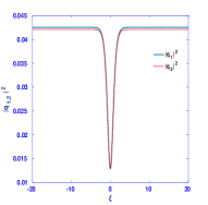
(a)

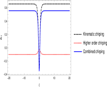
(b)

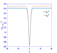
(c)

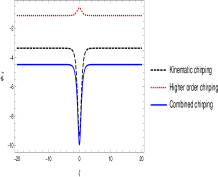
(d)

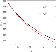
(e)

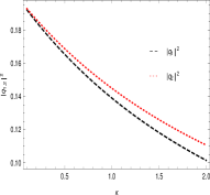
(f)

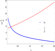
(g)

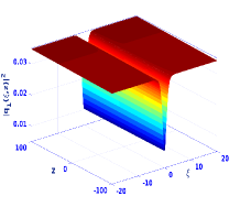
(h)

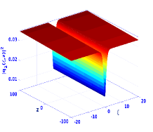
(i)

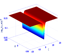
(j)

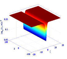
(k)

Figure 1: For Solution (16) (a)Plot of $|q_{1}|^{2}~{}\rm(blue~{}solid~{}line)$, $|q_{2}|^{2}~{}\rm(red~{}dotted~{}line)$ versus $\xi$ for $\beta=0.2,~{}\kappa=0.9,~{}v=0.5,~{}k_{1}=0.02,~{}k_{2}=0.01,~{}a_{5}=0.5,~{}c_{1}=-0.0169,~{}c_{2}=0.0166,~{}c_{3}=0.0839,~{}D=-2.2677$ at $z=5$ when $\bar{\sigma}_{1}=\bar{\sigma}_{2}=-1$, (b) Plot of kinematic chirping (black dashed line), higher order chirping (red dotted line) and combined chirping (blue solid line) of $q_{2}$ versus $\xi$ for $\kappa=0.5,~{}\beta=0.15,~{}a_{5}=0.5,~{}v=3.5,~{}k_{1}=0.8,~{}k_{2}=0.4,~{}c_{1}=-0.120755,~{}c_{2}=-0.0402516,~{}c_{3}=0.672854,~{}D=-2.45367$ when $\bar{\sigma}_{1}=\bar{\sigma}_{2}=-1$, (c) Plot of $|q_{1}|^{2}~{}\rm(blue~{}solid~{}line)$, $|q_{2}|^{2}~{}\rm(red~{}dotted~{}line)$ versus $\xi$ for $,~{}\beta=0.1,~{}\kappa=0.7,~{}v=0.1,~{}k_{1}=0.01,~{}k_{2}=0.03,~{}a_{5}=0.5,~{}c_{1}=0.0945,~{}c_{2}=-0.0972,~{}c_{3}=0.5808,~{}D=-1.0840$ at $z=5$ for $\bar{\sigma}_{1}=-\bar{\sigma}_{2}=1$, (d)Plot of kinematic chirping (black dashed line), higher order chirping (red dotted line) and combined chirping (blue solid line) of $q_{1}$ versus $\xi$ for $\kappa=0.7,~{}\beta=0.1,~{}a_{5}=0.5,~{}v=1.5,~{}k_{1}=0.01,~{}k_{2}=0.03,~{}c_{1}=-1.60271,~{}c_{2}=-1.64956,~{}c_{3}=1.03189,~{}D=-0.86813$ for $\bar{\sigma}_{1}=-\bar{\sigma}_{2}=1$, (e) Plot of $|q_{1}|^{2}~{}\rm(black~{}dashed~{}line)$, $|q_{2}|^{2}~{}\rm(red~{}dotted~{}line)$ versus $\kappa$ when $\bar{\sigma}_{1}=\bar{\sigma}_{2}=-1$ for $\beta=0.1,~{}v=0.5,~{}k_{1}=0.02,~{}k_{2}=0.01,~{}a_{5}=0.5,~{}\xi=5$, (f) Plot of $|q_{1}|^{2}~{}\rm(black~{}dashed~{}line)$, $|q_{2}|^{2}~{}\rm(red~{}dotted~{}line)$ versus $\kappa$ for $\beta=0.1,~{}v=0.1,~{}k_{1}=0.01,~{}k_{2}=0.03,~{}a_{5}=0.5,~{}\xi=5$ when $\bar{\sigma}_{1}=-\bar{\sigma}_{2}=1$, (g) Plot of $|v|$ (Blue solid line) versus $\kappa$ for $\beta=0.02$ and $\frac{1}{\beta}$ (Red dotted line) versus $\kappa$ for $v=0.5$. Other parameters are $k_{1}=0.3,~{}k_{2}=0.1,~{}D=-0.2$, (h)-(i) Simulation of the intensity profiles when $\bar{\sigma}_{1}=\bar{\sigma}_{2}=-1$ for the same parameter values as in (a), (j)-(k) Simulation of the intensity profiles when $\bar{\sigma}_{1}=\bar{\sigma}_{2}=-1$ for the same parameter values as in (c)

3.1.2 $0<D<1$: Anti-dark solitary wave

When $\bar{\sigma}_{1}=\bar{\sigma}_{2}=1$ (and $1+\alpha^{2}>\delta_{1}$), the intensity profiles of both the components of solution (20) with respect to $\xi$ are shown in Fig.2(a). Here the intensity decreases from the centre ($\xi=0$) similar to a bright soliton but approaches a constant intensity at infinity like a dark soliton. So it is a bright solitary wave on top of a non vanishing flat background i.e. an anti dark solitary wave [26] or following [27] it can also be termed as dark-like-bright solitary wave. Chirping reversal for the component $q_{2}$ is demonstrated in Fig.2(b). It is seen from Fig.2(c) that $|q_{1}|^{2}$ first increases then decreases as $\kappa$ increases but $|q_{2}|^{2}$ increases with increasing $\kappa$. Simulation of the intensity profiles of both the components as displayed in Figs.2(d) and (e) shows stable evolution of the solitary wave.

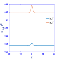
(a)

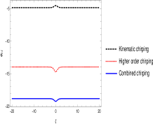
(b)

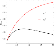
(c)

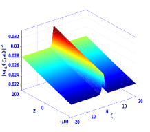
(d)

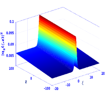
(e)

Figure 2: For Solution (16) when $\bar{\sigma}_{1}=\bar{\sigma}_{2}=1$ (a) Plot of $|q_{1}|^{2}~{}\rm(blue~{}solid~{}line)$, $|q_{2}|^{2}~{}\rm(red~{}dotted~{}line)$ versus $\xi$ for $\beta=0.1,~{}\kappa=0.9,~{}v=0.5,~{}k_{1}=-0.35,~{}k_{2}=0.3,~{}a_{5}=1.5,~{}c_{1}=0.3437,~{}c_{2}=-1.2178,~{}c_{3}=-0.5264,~{}D=0.1525$ at $z=5$, (b) Plot of kinematic chirping (black dashed line), higher order chirping (red dotted line) and combined chirping (blue solid line) of $q_{2}$ versus $\xi$ for $\kappa=0.9,~{}\beta=0.1,~{}a_{5}=1.5,~{}v=0.5,~{}k_{1}=-0.35,~{}k_{2}=0.3,~{}c_{1}=-0.613921,~{}c_{2}=-2.17542,~{}c_{3}=-5.55117,~{}D=0.0505951$, (c) Plot of $|q_{1}|^{2}~{}\rm(black~{}dashed~{}line)$, $|q_{2}|^{2}~{}\rm(red~{}dotted~{}line)$ versus $\kappa$ for $\beta=0.1,~{}v=0.5,~{}k_{1}=-0.35,~{}k_{2}=0.1,~{}a_{5}=1.5,~{}\xi=5$, (d)-(e) Simulation of the intensity profiles for parameter values as in (a)

3.2 Solution II

Another solution to Eqn.(16) is

$$\mu(\xi)=\frac{D+\rm sech(\xi)}{E+\rm sech(\xi)}\,,$$ (25)

provided

$$E=1\,,~{}~{}d_{1}=\frac{(5D+1)}{4(D-1)}\,,~{}~{}\eta_{1}A^{2}=-\frac{1}{D-1}\,,~{}~{}\frac{2c_{3}}{A^{2}}=\frac{D(2D+1)}{(D-1)}\,.$$ (26)

Note that this solution exists only if $D\neq 1$. It is then easy to show that for this solution $\beta^{2}$ is given by

$$\beta^{2}=\frac{4(D-1)[v^{2}+k_{1}+k_{2}+2\kappa(k_{1}k_{2}-k_{1}^{2}-k_{2}^{2})]}{(1+2\kappa v^{2})^{2}(1+5D)}$$ (27)

Using Eqn. (9), the chirping of the two components turns out to be

$$\delta\omega_{1}=-\left(\frac{v[1-2\kappa k_{1}]}{2\kappa v^{2}+1}+\frac{c_{1}\beta[1+sech(\xi)]}{A^{2}[D+sech(\xi)]}-\frac{4a_{5}A^{2}[D+sech(\xi)]}{[1+sech(\xi)](2\kappa v^{2}+1)}\right)\,,$$ (28)

$$\delta\omega_{2}=-\left(\frac{v[1-2\kappa k_{2}]}{2\kappa v^{2}+1}+\frac{c_{2}\beta[1+sech(\xi)]}{\alpha^{2}A^{2}[D+sech(\xi)]}-\frac{4a_{5}\alpha^{2}A^{2}[D+sech(\xi)]}{[1+sech(\xi)](2\kappa v^{2}+1)}\right)\,.$$ (29)

3.2.1 $D>1$ : Gray solitary waves

Appearance of gray solitary waves in both the components is seen in Fig.3(a) when $\bar{\sigma_{1}}=\bar{\sigma_{2}}=-1$. The chirping profile of the component $q_{2}$ with respect to $\xi$ as given in Fig.3(b) shows chirp reversal. Both the components of intensity decrease with $\kappa$ as can be seen from Fig.3(c). While the speed $|v|$ decreases as $\kappa$ increases, the pulse-width $\frac{1}{\beta}$ increases as $\kappa$ increases as shown in Fig.3(d). This behavior follows from Eqn.(27). So the speed can be decelerated by increasing $\kappa$. Results of numerical simulation as depicted in Figs.3(e), (f) demonstrate stable evolution of the solitary waves.

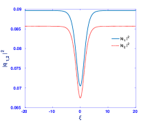
(a)

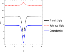
(b)

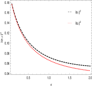
(c)

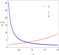
(d)

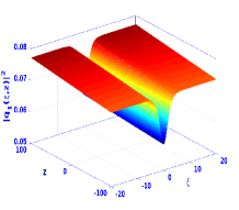
(e)

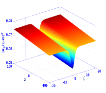
(f)

Figure 3: For Solution (25) when $\bar{\sigma}_{1}=\bar{\sigma}_{2}=-1$, (a) Plot of $|q_{1}|^{2}~{}\rm(blue~{}solid~{}line)$, $|q_{2}|^{2}~{}\rm(red~{}dotted~{}line)$ versus $\xi$ for $\beta=0.2,~{}\kappa=0.7,~{}v=1.5,~{}k_{1}=0.05,~{}k_{2}=0.01,~{}a_{5}=0.5,~{}c_{1}=-0.0238,~{}c_{2}=0.0224,~{}c_{3}=0.2707,~{}D=1.7147$ at $z=5$, (b) Plot of kinematic chirping (black dashed line), higher order chirping (red dotted line) and combined chirping (blue solid line) of $q_{2}$ versus $\xi$ for $\kappa=0.9,~{}\beta=0.4,~{}a_{5}=0.5,~{}v=0.5,~{}k_{1}=0.5,~{}k_{2}=0.35,~{}c_{1}=-0.0832854,~{}c_{2}=-0.0225096,~{}c_{3}=0.255425,~{}D=2.78374$, (c) Plot of $|q_{1}|^{2}~{}\rm(black~{}dashed~{}line)$, $|q_{2}|^{2}~{}\rm(red~{}dotted~{}line)$ versus $\kappa$ for $\beta=0.2,~{}v=1.5,~{}k_{1}=0.05,~{}k_{2}=0.01,~{}a_{5}=0.5,~{}\xi=5$, (d) Plot of $|v|$ (Blue solid line) versus $\kappa$ for $\beta=0.1$ and $\frac{1}{\beta}$ (Red dotted line) versus $\kappa$ for $v=0.75$. Other parameters are $k_{1}=0.5,~{}k_{2}=0.1,~{}D=2.1$. (e)-(f) Simulation of the intensity profiles for parameter values as in (a).

3.2.2 $0<D<1$: Anti-dark solitary waves

Appearance of anti-dark [26] or dark like bright solitary wave [27] in both the components is seen in Fig.4(a) when $\bar{\sigma_{1}}=\bar{\sigma_{2}}=1$ (and $1+\alpha^{2}>\delta_{1}$) and also when $\bar{\sigma_{1}}=-\bar{\sigma_{2}}=-1$ (and $\alpha^{2}>1+\delta_{1}$) as shown in Fig.4(c). Fig.4(b) shows chirping reversal for the component $q_{1}$ when $\bar{\sigma_{1}}=\bar{\sigma_{2}}=1$ and Fig.4(d) depicts the same for the component $q_{2}$ when $\bar{\sigma_{1}}=-\bar{\sigma_{2}}=-1$. Fig.4(e) shows that when $\bar{\sigma_{1}}=\bar{\sigma_{2}}=1$, $|q_{1}|^{2}$ first increases with increasing $\kappa$ but saturates when $\kappa$ nears the value $2$ whereas $|q_{2}|^{2}$ increases with $\kappa$. When $\bar{\sigma_{1}}=-\bar{\sigma_{2}}=-1$, Fig.4(f) demonstrates that, $|q_{1}|^{2}$ and $|q_{2}|^{2}$ increases with increasing $\kappa$. Simulation of the intensity profiles of both the components for $\bar{\sigma_{1}}=\bar{\sigma_{2}}=1$ (Figs.4(g),(h)) and for $\bar{\sigma_{1}}=-\bar{\sigma_{2}}=-1$ (Figs.4(i),(j)) shows the stable evolution and also the compression of both the components of the solitary waves.

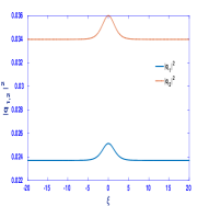
(a)

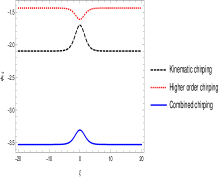
(b)

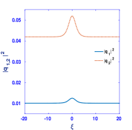
(c)

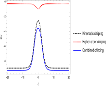
(d)

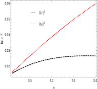
(e)

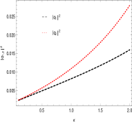
(f)

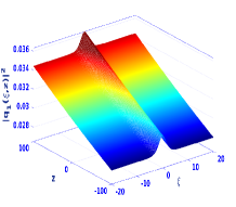
(g)

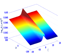
(h)

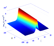
(i)

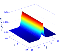
(j)

Figure 4: For Solution (25)   (a) Plot of $|q_{1}|^{2}~{}\rm(blue~{}solid~{}line)$, $|q_{2}|^{2}~{}\rm(red~{}dotted~{}line)$ versus $\xi$ for $\beta=0.1,~{}\kappa=0.9,~{}v=0.3,~{}k_{1}=-0.2,~{}k_{2}=0.05,~{}a_{5}=1.0,~{}c_{1}=0.4895,~{}c_{2}=-0.7315,~{}c_{3}=-0.2828,~{}D=0.8818$ at $z=5$ when when $\bar{\sigma}_{1}=\bar{\sigma}_{2}=1$, (b) Plot of kinematic chirping (black dashed line), higher order chirping (red dotted line) and combined chirping (blue solid line) of $q_{1}$ versus $\xi$ for $\kappa=0.9,~{}\beta=0.3,~{}a_{5}=1.0,~{}v=0.5,~{}k_{1}=-0.2,~{}k_{2}=0.1,~{}c_{1}=-0.570754,~{}c_{2}=-0.946616,~{}c_{3}=-1.04094,~{}D=0.804471$ when $\bar{\sigma}_{1}=\bar{\sigma}_{2}=1$, (c) Plot of $|q_{1}|^{2}~{}\rm(blue~{}solid~{}line)$, $|q_{2}|^{2}~{}\rm(red~{}dotted~{}line)$ versus $\xi$ for $,~{}\beta=0.1,~{}\kappa=0.9,~{}v=0.2,~{}k_{1}=-0.1,~{}k_{2}=0.4,~{}a_{5}=4.5,~{}c_{1}=0.0726,~{}c_{2}=-0.3058,~{}c_{3}=-0.0315,~{}D=0.6708$ at $z=5$ when $\bar{\sigma}_{1}=-\bar{\sigma}_{2}=-1$, (d) Plot of kinematic chirping (black dashed line), higher order chirping (red dotted line) and combined chirping (blue solid line) of $q_{2}$ versus $\xi$ for $\kappa=0.9,~{}\beta=0.4,~{}a_{5}=1.0,~{}v=0.5,~{}k_{1}=-0.1,~{}k_{2}=0.4,~{}c_{1}=-0.0978927,~{}c_{2}=-0.412548,~{}c_{3}=-0.00882376,~{}D=0.180327$ when $\bar{\sigma}_{1}=-\bar{\sigma}_{2}=-1$, (e) Plot of $|q_{1}|^{2}~{}\rm(black~{}dashed~{}line)$, $|q_{2}|^{2}~{}\rm(red~{}dotted~{}line)$ versus $\kappa$ for $\beta=0.1,~{}v=0.3,~{}k_{1}=-0.2,~{}k_{2}=0.05,~{}a_{5}=1.0,~{}\xi=5$ when when $\bar{\sigma}_{1}=\bar{\sigma}_{2}=1$, (f) Plot of $|q_{1}|^{2}~{}\rm(black~{}dashed~{}line)$, $|q_{2}|^{2}~{}\rm(red~{}dotted~{}line)$ versus $\kappa$ for $\beta=0.05,~{}v=0.2,~{}k_{1}=-0.1,~{}k_{2}=0.05,~{}a_{5}=4.5,~{}\xi=5$ when $\bar{\sigma}_{1}=-\bar{\sigma}_{2}=-1$, (g)-(h) Simulation of the intensity profiles for parameter values as in (a) when $\bar{\sigma}_{1}=\bar{\sigma}_{2}=1$, (i)-(j) Simulation of the intensity profiles when $\bar{\sigma}_{1}=-\bar{\sigma}_{2}=-1$ for parameter values same as (c).

4 Conclusion

In this article the nonlinear coupled cubic Helmholtz system in the presence of non-Kerr terms like the self steepening and the self frequency shift is considered. This system describes nonparaxial pulse propagation with Kerr and non-Kerr nonlinearities with spatial dispersion originating from the nonparaxial effect that becomes dominant when the slowly varying envelope approximation fails. We have shown that this coupled cubic Helmholtz equations, in the presence of the self steepening and the self frequency shift, admit exact chirped gray and anti-dark solitary wave solutions (depending on the nature of nonlinearity) both of which show not only chirping but also chirp reversal for a particular combination of the self steepening and the self frequency shift parameters. This is the novel physical effect resulting from the inclusion of non Kerr nonlinearity into the cubic coupled Helmholtz system. In particular, so long as $a_{4}=2a_{5}$, the nonlinear chirp of both the gray and anti-dark solitary waves consists of two terms, one (on account of non Kerr terms) is directly proportional to the intensity of the solitary wave while the other is inversely proportional to the intensity, thereby giving rise to chirp reversal. On the other hand, when $3a_{4}+2a_{5}=0$, then the solutions show only chirping but no chirp reversal. Physical significance of the obtained solutions are explored by examining the effect of nonparaxial parameter on intensity, speed and pulse width of the solitary waves. It is found that the speed of the solitary wave can be tuned by altering the nonparaxial parameter. The stability of the exact solutions has been studied by means of direct simulations of the perturbed evolution of the solutions and are found to be stable for the parametric regions examined herein. The present study is likely to provide a key analytical platform in the understanding of the nonparaxial chirped vector soliton interaction [8]. The nonlinearly chirped solutions presented here may find applications in nonparaxial optical contexts where pre chirp managed femtosecond pulses are used e.g. in fiber optic communication systems, nonlinear optical fiber amplifiers/compressors [20, 23].
This work paves the way for future directions of study. It is of natural interest to investigate coupled cubic-quintic Helmholtz system with non-Kerr nonlinearity. Looking for the possibility of chirped solitons for spatially or spatio temporally modulated nonlinearity could be of considerable research interest. To search for multi-hump solutions [24], rogue waves in the present scenario is another area worth investigating. Modulation instability in the presence of the self steepening and the self frequency shift is an important topic which deserves investigation. Some of these issues are being examined and we hope to report on some of these issues in the near future.

Data Availability
Data sharing is not applicable to this article as no new data were created or analyzed in this study.

References

- [1] B.Crosignani, A.Cutolo, P.D.Porto, J. Opt. Soc. Am. 72, 1136 (1982); F.Poletti, P.Horak, J.Opt.Soc.Am. B 25, 1645 (2008); C.R.Menyuk, IEEE J. Quantum Electron. 25, 2674 (1989)
- [2] Y.S.Kivshar, Opt.Quantum Electron. 30, 571 (1998); Y.S.Kivshar and B.Luther Davies, Phys.Rep.298, 81 (1998); G.Stegeman and M.Segev, Science 286, 1518 (1999)
- [3] S.V.Manakov, Sov.Phys.JETP 38, 248 (1974)
- [4] P.Chamorro-Posada, G.S.McDonald and G.H.C.New, J.Opt.Soc.Am.B 19, 1216 (2002)
- [5] S.Chi and Q.Guo, Opt.Letts. 20, 1598 (1995); A.Ciattoni, P.Di Porto, B.Crosignani and A.Yariv, J.Opt.Soc.Am.B 17, 809 (2000); B.Crosignani, A.Yariv and S.Mookherjea, Opt.Lett. 29, 1524 (2004); A.Ciattoni, B.Crosignani, S.Mookherjea and A.Yariv, Opt.Lett. 30, 516 (2005); A.Ciattoni, B.Crosignani, P.Di Porto, J.Scheuer and A.Yariv, Opt.Exp. 14, 5517 (2006)
- [6] M.Lax, W.H.Louisell and W.B.McKnight, Phys.Rev.A 11, 1365 (1975)
- [7] P.Chamorro-Posada, G.S.McDonald and G.H.C.New, J.Mod.Opt. 45, 1111 (1998); J.M.Christian, G.S.McDonald, R.J.Potton and P.Chamorro-Posada, Phys.Rev.A 76, 033833(2007);
- [8] P.Chamorro-Posada and G.S.McDonald, Phys.Rev.E 74, 036609 (2006)
- [9] P.Chamorro-Posada and G.S.McDonald, Opt.Lett. 28, 825 (2003); J.M.Christian, E.A.McCoy, G.S.McDonald, P.Chamorro-Posada, J.Atom.Mol.Opt.Phys. 2012, 137967 (2012); J.M.Christian, G.S.Mcdonald, P. Chamorro-Posada, J.Phys.A: Math.Theor. 40, 1545 (2007); J.M.Christian, G.S.McDonald, T.F.Hodgkinson and P.Chamorro-Posada, Phys.Rev.A 86, 023838 (2012); J.M.Christian, G.S.McDonald, T.F.Hodgkinson and P.Chamorro-Posada, Phys.Rev.A 86, 023839 (2012)
- [10] K.Tamilselvan, T.Kanna and A.Govindarajan, Chaos 29, 063121 (2019)
- [11] J.M.Christian, G.S.Macdonald, P.Chamorro-Posada, Phys.Rev.E 74, 066612 (2006)
- [12] D.Anderson and M.Lisak, Opt.Lett. 7, 394 (1982)
- [13] J.R.de Oliveira and M.A.de Moura, Phys.Rev.E 57, 4751 (1998)
- [14] Yuri S.Kivshar , Govind P.Agrawal, Optical Solitons: From Fibres to Photonic Crystals (Academic Press, Boston, 2001)
- [15] F.M.Mitschke and L.F.Mollenauer, Opt.Lett. 11, 659 (1986); J.P.Gordon, Opt.Lett. 11, 662 (1986)
- [16] S.Blair, Chaos 10, 570 (2000)
- [17] K.Tamilselvan, T.Kanna, Avinash Khare, Commun.Nonl.Sci.Num.Sim. 39, 134 (2016)
- [18] M.Kumar, N.Nithyanandan, H.Triki, K.Porsezian, Optik 182, 1120 (2019)
- [19] V.I.Kruglov, A.C.Peacock and J.D.Harvey, Phys.Rev.Lett. 90, 113902 (2003)
- [20] S.T.Cundiff et al, Jour.Lightwave.Tech. 17, 811 (1999)
- [21] L.V.Hmurcik and D.J.Kaup, J.Opt.Soc.Am. 69, 597 (1979); M.Desaix, L.Helczynski, D.Anderson, and M.lisak, Phys.Rev.E 65, 056602 (2002); M.Neuer, K.H.Spatschek and Z.Li, Phys.Rev.E 70, 056605 (2004); Alka, A.Goyal, R.Gupta, C.N.Kumar and T.S.Raju, Phys.Rev.A 84, 063830 (2011); V.M.Vyas, P.Patel, P.K.Panigrahi, C.N.Kumar and W.Greiner, Phys.Rev.A 78, 021803(R) (2008); H.Triki, K.Porsezian, A.Choudhuri and P.T.Dinda, Phys.Rev.A 93, 063810 (2016); V.I.Kalashnikov, Phys.Rev.E 80, 046606 (2009); S.Chen, F.Baronio, J.M.Soto-Crespo, Y.Liu, and P.Grelu, Phys.Rev.A 93, 062202 (2016)
- [22] G.P.Agrawal, Nonlinear Fiber Optics (Academic, Boston, 2001)
- [23] R.Chen and G.Chang, J.Opt.Soc.Am.B 37, 2388 (2020)
- [24] E.A.Ostrovskaya and Y.S.Kivshar, J.Opt.B: Quantum and Semiclassical Optics, 1, 77 (1999); E.A.Ostrovskaya, Y.S.Kivshar, D.V.Skyrabin and W.J.Firth, Phys.Rev.Lett. 83, 296 (1999)
- [25] Y.S.Kivshar, IEEE J.Quantum Electron. 28, 250 (1993)
- [26] K.Manikandan, N.Vishnu Priya, M.Senthilvelan and R.Sankaranarayanan, CHAOS 28, 083103 (2018)
- [27] Y.S.Kivshar, V.V.Afansjev, A.W.Snyder, Opt.Commun. 126, 348 (1996)