Towards top-down holographic composite Higgs: minimal coset from maximal supergravity

Abstract

Within the context of top-down holography, we study a one-parameter family of regular background solutions of maximal gauged supergravity in seven dimensions, dimensionally reduced on a 2-torus. The dual, four-dimensional confining field theory realises the global (spontaneous as well as explicit) symmetry breaking pattern $SO(5)\rightarrow SO(4)$. We compute the complete mass spectrum for the fluctuations of the 128 bosonic degrees of freedom of the five-dimensional gravity theory, which correspond to scalar, pseudoscalar, vector, axial-vector, and tensor bound states of the dual field theory, and includes particles with exotic $SO(4)$ quantum numbers. We confirm the existence of tachyonic instabilities near the boundaries of the parameter space.

We discuss the interplay between explicit and spontaneous symmetry breaking. The $SO(5)/SO(4)$ coset might provide a first step towards the realisation of a calculable framework and ultraviolet completion of minimal composite Higgs models, if the four pseudo-Nambu-Goldstone bosons are identified with the real components of the Higgs doublet in the standard model (SM), and a subgroup of $SO(4)$ with the $SU(2)\times U(1)$ SM gauge group. We exhibit an example with an additional localised boundary term that mimics the effect of a weakly-coupled external sector.

1 Introduction

After the discovery of the Higgs boson Aad:2012tfa ; Chatrchyan:2012xdj , and in preparation for the restart of the experimental programme of the Large Hadron Collider (LHC), renewed attention in the literature has focused on Composite Higgs Models (CHMs) Kaplan:1983fs ; Georgi:1984af ; Dugan:1984hq . In such scenarios, the standard-model (SM) Higgs doublet scalar fields would arise as pseudo-Nambu-Goldstone Bosons (pNGBs) in the low-energy Effective Field Theory (EFT) description of a more fundamental theory. It is usually assumed that the underlying dynamics be strongly coupled, leading to the formation of infinitely many bound states. An overview of the field is provided by the reviews in Refs. Panico:2015jxa ; Witzel:2019jbe ; Cacciapaglia:2020kgq , and by the useful summary tables in Refs. Ferretti:2013kya ; Ferretti:2016upr ; Cacciapaglia:2019bqz (see also the selection of useful papers in Refs. Contino:2003ve ; Agashe:2004rs ; Katz:2005au ; Agashe:2005dk ; Agashe:2006at ; Contino:2006qr ; Barbieri:2007bh ; Lodone:2008yy ; Falkowski:2008fz ; Gripaios:2009pe ; Mrazek:2011iu ; Contino:2011np ; Marzocca:2012zn ; Grojean:2013qca ; Barnard:2013zea ; Cacciapaglia:2014uja ; Ferretti:2014qta ; Arbey:2015exa ; vonGersdorff:2015fta ; Cacciapaglia:2015eqa ; Feruglio:2016zvt ; DeGrand:2016pgq ; Fichet:2016xvs ; Galloway:2016fuo ; Agugliaro:2016clv ; Belyaev:2016ftv ; Bizot:2016zyu ; Csaki:2017cep ; Chala:2017sjk ; Golterman:2017vdj ; Csaki:2017jby ; Alanne:2017rrs ; Alanne:2017ymh ; Sannino:2017utc ; Alanne:2018wtp ; Bizot:2018tds ; Cai:2018tet ; Agugliaro:2018vsu ; Cacciapaglia:2018avr ; Gertov:2019yqo ; Ayyar:2019exp ; Cacciapaglia:2019ixa ; BuarqueFranzosi:2019eee ; Cacciapaglia:2019dsq ; Cacciapaglia:2020vyf , and references therein).

We want to study the strong-coupling dynamics underlying CHMs, and address calculability (from first principles), in particular for observable quantities of phenomenological relevance, such as the mass spectra of bound states. One possible approach to this endeavour is provided by lattice gauge theory. There exist lattice studies of $SU(2)$ Hietanen:2014xca ; Detmold:2014kba ; Arthur:2016dir ; Arthur:2016ozw ; Pica:2016zst ; Lee:2017uvl ; Drach:2017btk ; Drach:2020wux and $Sp(4)$ Bennett:2017kga ; Bennett:2019jzz ; Bennett:2019cxd gauge theories that explore the fundamental origin of CHMs based on the $SU(4)/Sp(4)$ coset Barnard:2013zea , as well as lattice explorations with $SU(4)$ gauge group Ayyar:2017qdf ; Ayyar:2018zuk ; Ayyar:2018ppa ; Ayyar:2018glg ; Cossu:2019hse aimed at capturing some of the dynamical features of models based on the $SU(5)/SO(5)$ coset. Ref. Appelquist:2020bqj shows that salient features of CHMs based upon $SU(N_{f})\times SU(N_{f})/SU(N_{f})$ cosets (see also Refs. Vecchi:2015fma ; Ma:2015gra ; BuarqueFranzosi:2018eaj ) are captured by the lattice studies of the $SU(3)$ gauge theory with $N_{f}=8$ Dirac fermions in the fundamental representation Aoki:2014oha ; Appelquist:2016viq ; Aoki:2016wnc ; Gasbarro:2017fmi ; Appelquist:2018yqe , via the application of the dilaton EFT Matsuzaki:2013eva ; Golterman:2016lsd ; Kasai:2016ifi ; Hansen:2016fri ; Golterman:2016cdd ; Appelquist:2017wcg ; Appelquist:2017vyy ; Golterman:2018mfm ; Cata:2019edh ; Appelquist:2019lgk ; Golterman:2020tdq .

The $SO(5)/SO(4)$ minimal coset has dimension four and includes custodial symmetry. It is natural to identify the pNGBs, transforming as $4$ of $SO(4)$, with the Higgs doublet in the standard model Agashe:2004rs . Yet, this coset is conspicuous by its absence in the list of current lattice explorations, as summarised in the previous paragraph. It is not trivial to provide a dynamical origin for CHMs based on this coset, in terms of familiar gauge theories with fermionic matter. An example is provided by Ref. Caracciolo:2012je , which beautifully exploits supersymmetry and Seiberg duality, though subject to the usual limitations in terms of calculability within this approach.

A radically different approach to address calculability in strongly coupled gauge theories adopts gauge-gravity dualities (holography) Maldacena:1997re ; Gubser:1998bc ; Witten:1998qj ; Aharony:1999ti . The large-$N$ limit of special strongly-coupled gauge theories is equivalent to a weakly-coupled theory of gravity in extra dimensions, amenable to perturbative treatment. Interesting observables are recovered by applying the dictionary of the correspondence—which requires the implementation of holographic renormalisation Bianchi:2001kw ; Skenderis:2002wp ; Papadimitriou:2004ap . Global symmetries of the field theory are generically realised as gauge symmetries in the bulk of the gravity theory. Hence, the starting point for the realisation of the dynamics of CHMs with an $SO(5)/SO(4)$ coset should be a higher-dimensional theory of gravity supplemented by $SO(5)$ gauge symmetry.

An extensive body of work (see for instance Refs. Contino:2003ve ; Agashe:2004rs ; Agashe:2005dk ; Agashe:2006at ; Contino:2006qr ; Falkowski:2008fz ; Contino:2011np ) demonstrate the reach of the bottom-up approach to holography in building a realisation of the CHMs with $SO(5)/SO(4)$ coset. By choosing a fixed curved background in $D=5$ dimensions, and a set of fields propagating in this background, it is possible to capture the salient features of the dynamics of the pNGBs and some of the spin-1/2 and spin-1 composite particles. The spontaneous symmetry breaking $SO(5)\rightarrow SO(4)$ is implemented by means of appropriate choices of the field content, background, and boundary conditions. While calculability is greatly improved by this approach, important properties of the long distance dynamics are not captured by bottom-up models: for example, demonstrating confinement requires embedding the gravity theory in string theory, hence allowing for the holographic treatment of the Wilson loops Rey:1998ik ; Maldacena:1998im (see also Refs. Kinar:1998vq ; Brandhuber:1999jr ; Avramis:2006nv ; Nunez:2009da ; Faedo:2013ota ) to recover the area law, as suggested in Ref. Witten:1998zw . Furthermore, top-down models fix the relation between masses of the resonances in a predictive way, as it emerges from the dual strong dynamics.

Recently, inspired by sophisticated holographic models exhibiting QCD-like properties (such as the Sakai-Sugimoto model Sakai:2004cn ; Sakai:2005yt and its precursors Karch:2002sh ; Kruczenski:2003be ; Erdmenger:2007cm ), new bottom-up holographic realisations of CHMs have been developed Erdmenger:2020lvq ; Erdmenger:2020flu . The same coset structures studied on the lattice are here realised by bulk fields, inspired by the DBI action that describes extended objects probing the curved background (and captures the quenched approximation for matter fields in the large-$N$ limit of the field theory). In a parallel direction, Ref. Elander:2020nyd includes deformations to mimic the backreaction due to many such extended objects (edging towards the Veneziano limit of the large-$N$ field theory).

With this paper, we propose an alternative approach, closer in spirit to the original holographic dualities. Known supergravity theories can provide complete top-down holographic models, in which the strong-coupling field-theory dynamics is fully captured. We consider supergravities that include at their core the interesting (gauged) symmetry group, without the need for additional matter fields and/or stacks of $Dp$-branes. The resulting enhanced calculability is a double-edged sword: while the fact that the field content and phenomenology are rigidly dictated by supergravity leads to greater predictability, it also makes the task of identifying realistic models a more challenging endeavour. We exemplify this programme with the maximal $SO(5)$ gauged supergravity theory in seven dimensions, within which we realise the $SO(5)/SO(4)$ coset of a minimal CHM.

In the rest of this introduction, we summarise the main features of the model, as they emerge from the relevant technical literature. Our starting point is the established fact that maximal supergravity in seven dimensions has a gauged $SO(5)$ symmetry Pilch:1984xy ; Nastase:1999cb ; Pernici:1984xx ; Pernici:1984zw ; Cvetic:1999xp ; Lu:1999bc ; Campos:2000yu ; Cvetic:2000ah ; Samtleben:2005bp . It can be obtained by dimensional reduction on $S^{4}$ of maximal supergravity in $D=11$ dimensions, and the $SO(5)$ originates from the isometry group of the $S^{4}$. The background solution with AdS${}_{7}\times S^{4}$ geometry is interpreted, in the language of gauge-gravity dualities, in terms of the somewhat mysterious ${\cal N}=(2,0)$ strongly coupled gauge theory living on a stack of $M5$-branes, which is a superconformal chiral theory with extended supersymmetry. While the microscopic details of this field theory are not known in general terms, many of its properties are established in the literature—for example $SO(5)$ is indeed its global R-symmetry—and an incomplete selection of interesting studies can be found in Refs. Ganor:1996nf ; Witten:1996hc ; Seiberg:1997ax ; Aharony:1997an ; Harvey:1998bx ; Corrado:1999pi ; Intriligator:2000eq ; Cordova:2015vwa .

One reason why this obsure field theory, and its emergence as the dual of a special solution in supergravity, is of interest, in the literature on gauge/gravity dualities, is the observation in Ref. Witten:1998zw that one can identify background solutions in which two of the dimensions are compactified on circles, one of which connects the lifts to eleven-dimensional supergravity and to type-IIA supergravity in ten dimensions. Solutions in which the other circle—along which fermions have anti-periodic boundary conditions, breaking supersymmetry—shrinks to zero size, at some finite value of the radial direction ($\rho\rightarrow\rho_{o}$) in the geometry, yield in the dual field theory the long distance behaviour of a confining theory in four dimensions. Not only is there a mass gap, but furthermore the holographic calculation of the appropriate rectangular Wilson loops Rey:1998ik ; Maldacena:1998im (see also Refs. Kinar:1998vq ; Brandhuber:1999jr ; Avramis:2006nv ; Nunez:2009da ; Faedo:2013ota ), yields a static potential that grows linearly with the displacement between two heavy quarks. This class of curved backgrounds underlies the $D4/D8$ system exploited in the aforementioned Sakai-Sugimoto holographic model of quenched QCD Sakai:2004cn ; Sakai:2005yt .

As a distinctive feature, we do not add probe branes to the smooth geometries that we study, but instead implement the global symmetry breaking pattern by considering the supergravity theory on its own. We recall some of the salient aspects of this supergravity theory here, deferring the technical details to the appropriate sections of the main body of the paper. The scalar manifold of the supergravity theory describes the 14-dimensional (right) coset $SL(5,\mathbb{R})/SO(5)_{c}$, and the scalars transform (on the left) as a 2-index symmetric traceless representation of the gauged $SO(5)$. It has been known from the onset Pernici:1984zw of the study of this theory that background solutions exist in which one scalar $\phi$ has a non-trivial radial profile, breaking conformal symmetry, supersymmetry, and $SO(5)$ to its $SO(4)$ subgroup. The dynamics of $\phi$, in particular in relation to the dilatation operator in the dual field theory, has been discussed extensively, for example in Refs. Elander:2013jqa ; Elander:2020csd ; Elander:2020fmv and references therein, for a wide variety of admissible backgrounds. The symmetric traceless representation of $SO(5)$ decomposes as $14\rightarrow 1\oplus 4\oplus 9$ of $SO(4)$. The $4$ pNGBs describe the $SO(5)/SO(4)$ coset, and hence these backgrounds provide a dynamical realisation of the coset structure underlying the minimal CHM in Ref. Agashe:2004rs , as desired. The analysis of the UV asymptotics of the background shows that $SO(5)$ is broken both explicitly as well as spontaneously.

Besides observing that this structure matches the one postulated in the minimal CHM, our main contribution is the calculation of the spectra of fluctuations of all bosonic fields obtained after dimensional reduction on a 2-torus, performed by adopting the formalism developed in Refs. Bianchi:2003ug ; Berg:2005pd ; Berg:2006xy ; Elander:2009bm ; Elander:2010wd . We further generalise the results of Refs. Brower:2000rp to a whole class of backgrounds, and to include the whole spectrum of $p$-forms, for which we make use of the $R_{\xi}$ gauge, along the lines of Ref. Elander:2018aub . There are $23$ independent towers of such bosonic eigenstates, with various degrees of degeneracy governed by the unbroken $SO(4)$ symmetry, that make up the 128 bosonic degrees of freedom of maximal supergravity.

For the time being, we ignore two model-dependent aspects of the theory, that are not central to the construction: we consider only the bosonic field content, while ignoring completely the fermions, and we also disregard the interactions descending from the Chern-Simons terms, as they do not affect the calculation of the spectra of bound states. The spectrum of fermionic bound states in the field theory depends on how the compactification breaks supersymmetry. We focus instead on model-independent parts of the spectrum, directly related to the underlying symmetries. The embedding of the standard model $SU(2)\times U(1)$ group must be anomaly free, a requirement that, as in other CHMs, may be subtle, but not hard to satisfy. We postpone to future studies any phenomenological considerations, starting from the detailed implementation of the procedure allowing to (weakly) gauge the $SU(2)\times U(1)$ subgroup of $SO(4)$—which involves some subtlety in the process of holographic renormalisation—as well as the coupling to the standard-model matter fields, and the vacuum (mis-)alignment features leading to electroweak symmetry breaking.

Finally, we notice that similar constructions can in principle be applied also in other classes of supergravities. For example, in the context of the half-maximal supergravity in six dimensions, coupled to $n$ vector multiplets Romans:1985tw ; Romans:1985tz ; Brandhuber:1999np ; Cvetic:1999un ; Samtleben:2005bp (see also Refs. Hong:2018amk ; Jeong:2013jfc ; DAuria:2000afl ; Andrianopoli:2001rs ; Nishimura:2000wj ; Ferrara:1998gv ; Gursoy:2002tx ; Nunez:2001pt ; Karndumri:2012vh ; Lozano:2012au ; Karndumri:2014lba ; Chang:2017mxc ; Gutperle:2018axv ; Suh:2018tul ; Suh:2018szn ; Kim:2019fsg ; Chen:2019qib ; Hoyos:2020fjx ), and compactified on a circle Wen:2004qh ; Kuperstein:2004yf ; Elander:2013jqa ; Elander:2018aub . Solutions to these systems exist that admit an interpretation of the long distance dynamics in terms of confining field theories in four dimensions. The scalar manifold describes the non-trivial and non-compact $O(1,1)\times O(4,n)/(SO(4)\times O(n))$ coset—though it is not immediately apparent how to embed an interesting CHM into this coset. Alternatively, in the case of these six-dimensional supergravities it has been shown that the existence of different lifts to ten dimensions can lead to interesting structures in the dual field theory, with additional flavor symmetry emerging non-trivially Legramandi:2021aqv .

The paper is organised as follows. In Sec. 2 we define the supergravity theory in $D=7$ dimensions, discussing its field content, couplings, and free parameters. Most of the material is lifted from the literature, but we find it useful to fix the notation used in the rest of the paper. In Sec. 3 we perform the reduction on a torus and write the resulting action in $D=5$ dimensions, including all the bosonic degrees of freedom, substantially extending available results in the literature. In Sec. 3.1 we display the class of solutions we are interested in, by analysing their asymptotic behaviours and hence illustrating the process that allows to generate them numerically. We demonstrate that the solutions are regular, and discuss what we mean by stating that the dual theory confines. In Sec. 4, we compute the mass spectrum. We start with the linearised equations of gauge invariant combinations of fluctuations of the metric and of the background scalars in Sec. 4.1. This section extends and completes some of the results presented in Refs. Elander:2013jqa ; Elander:2020csd ; Elander:2020fmv . In Secs. 4.2, 4.3, and 4.4 we complete the study of the bosonic mass spectrum, by looking at the fields that are trivial in the background. We discuss the spectra of $p$-forms, with $p=0,1,2$. We adopt a generalisation of the $R_{\xi}$ gauge to gauge-fix the theory (see also Ref. Elander:2018aub ), and present our numerical results, commenting on the treatment of numerical artefacts, where appropriate. In Sec. 5, after summarising the main features of the mass spectrum, we study its dependence on the free adjustment of boundary-localised terms that preserve the SO(4) symmetry of the system, but may introduce additional explicit breaking of SO(5). We focus on one particular example of such an admissible term, that affects the pNGBs and the lightest spin-1 composite states in the dual theory. In Sec. 6 we summarise our main findings and outline an extensive programme of future investigations.

We relegate to the Appendix an extensive selection of technical details, that can be skipped at first reading of the paper, but would be useful to reproduce our results, or to apply the same formalism to other classes of background solutions. We devote Appendix A to discussing the self-duality condition of the $3$-forms in seven dimensions, and its consequences for the $2$-forms in five dimensions. Appendix B contains technical details about the background solutions and the formalism in which we treat the fluctuations, including the asymptotic expansions of the fluctuations. Appendix C summarises some elements of the lift to ten- and eleven-dimensional supergravity, borrowed from the literature. We also observe that the result of the holographic calculation of the string tension suggests the existence of a discontinuity, the energetically favoured string configurations qualitatively differing, depending on the sign of $\phi$. We leave this observation for future investigations.

We close the paper with Appendix D, in which we summarise our numerical results for the whole spectrum of the toroidal compactification, but now in the case of unbroken $SO(5)$. We critically compare our results to those of Ref. Brower:2000rp , who considered the same $SO(5)$-invariant background, but used a different formalism and restricted their analysis to a different set of supergravity modes. We find good agreement between the two sets of results, in the common sector, thus providing a useful cross check. Unsurprisingly, we also find that several of the states in our study, that represent non-trivial $SO(5)$ multiplets, are lighter than the singlets one would retain in a consistent truncation.

2 Maximal gauged supergravity in seven dimensions

The field content and action of maximal supergravity in $D=7$ dimensions are discussed for example in Refs. Nastase:1999cb ; Pernici:1984xx ; Pernici:1984zw ; Cvetic:1999xp ; Lu:1999bc ; Cvetic:2000ah (see also Refs. Samtleben:2005bp ; Campos:2000yu ; Elander:2013jqa ; Cowdall:1998rs ). The seven-dimensional space-time indexes are denoted by $\hat{M}=0,\,1,\,2,\,3,\,5,\,6,\,7$, while we use the Greek indexes $\alpha=1\,,\cdots\,,5$ to denote the components of the fundamental representation of the $SO(5)$ gauge group. The bosonic fields in the weakly-coupled action are the following (counting on-shell degrees of freedom): $14$ real scalars, $10$ (massless) vectors ${\cal A}_{\hat{M}\,\alpha}^{\,\,\,\,\,\,\,\,\,\,\beta}$ (each propagating $5$ real degrees of freedom), $5$ (massive self-dual) $3$-forms $S_{\hat{M}\hat{N}\hat{P}\,\alpha}$ (each propagating $10$ real degrees of freedom, rather than $20$, because their equation of motion is the first-order self-duality condition), and the metric ($14$ degrees of freedom). The $128$ degrees of freedom match the fermionic field content, which consists of $16$ gauginos ($4$ complex components each) and $4$ gravitinos ($(D-3)2^{[D/2]}/2=16$ degrees of freedom each).

The scalar manifold describes the $SL(5,\mathbb{R})/SO(5)_{c}$ right coset, and we label by $i,j=1,\,\cdots\,,5$ the fundamental representation of the global $SO(5)_{c}$ symmetry, to retain the distinction with the indexes of the gauged $SO(5)$. The $14$ scalars parametrising the coset are written in terms of a $5\times 5$ real unit-determinant matrix $\Pi_{\alpha}^{\,\,\,\,i}$ (with ${\rm det}(\Pi_{\alpha}^{\,\,\,\,i})=1$), that transforms under the action of $SO(5)_{c}$ on the right, and of $SO(5)$ on the left. The $10$ vectors transform as the adjoint of $SO(5)$, and the $3$-forms in the fundamental. Because $SO(5)\simeq Sp(4)$, the gravitinos transform in the spinorial $4$-dimensional representation of $SO(5)_{c}$, while the gauginos transform as the irreducible part of the product of the vectorial and the spinorial representation of $SO(5)_{c}$ (as $5\otimes 4\rightarrow 16\oplus 4$ in $Sp(4)$ Yamatsu:2015npn ). We ignore fermions from here on.

The bosonic part of the action is the following:

$${\cal S}_{7} = \int\mbox{d}^{7}x\left\{\sqrt{-\hat{g}_{7}}\left[\frac{{\cal R}_{7}}{4}-\frac{1}{4}\hat{g}^{\hat{M}\hat{N}}\delta^{ik}\delta_{j\ell}P_{\hat{M}\,i}^{\,\,\,\,\,\,\,\,\,\,j}P_{\hat{N}k}^{\,\,\,\,\,\,\,\,\,\ell}-\frac{m^{2}}{8}\left(2\delta^{i}_{\,\,\,k}\delta^{j}_{\,\,\,\ell}-\delta^{ij}\delta_{k\ell}\right)T_{ij}T^{k\ell}+\right.\right.$$

$$\left.\left.\frac{}{}+\frac{1}{8}\left(\Pi_{\alpha}^{\,\,\,i}\Pi_{\beta}^{\,\,\,j}{\cal F}^{\alpha\beta}_{\hat{M}\hat{N}}\right)^{2}-\frac{m^{2}}{4}\Big{(}(\Pi^{-1})_{i}^{\,\,\,\alpha}S_{\hat{M}\hat{N}\hat{O}\,\alpha}\Big{)}^{2}\right]\right.+$$

$$\left.\frac{}{}+\frac{m}{96}\epsilon^{\hat{M}\hat{N}\hat{O}\hat{P}\hat{Q}\hat{R}\hat{S}}S_{\hat{M}\hat{N}\hat{O}\,\alpha}\delta^{\alpha\beta}F^{(S)}_{\hat{P}\hat{Q}\hat{R}\hat{S}\,\beta}\right.+$$

$$\left.\frac{}{}-\frac{i}{32\sqrt{3}}\epsilon^{\hat{M}\hat{N}\hat{O}\hat{P}\hat{Q}\hat{R}\hat{S}}\epsilon_{\alpha\beta\gamma\delta\eta}\delta^{\alpha\alpha^{\prime}}S_{\hat{M}\hat{N}\hat{O}\,\alpha^{\prime}}\delta^{\beta\beta^{\prime}}{\cal F}_{\hat{P}\hat{Q}\,\beta^{\prime}}^{\,\,\,\,\,\,\,\,\,\,\,\,\,\,\gamma}\delta^{\delta\delta^{\prime}}{\cal F}_{\hat{R}\hat{S}\,\delta^{\prime}}^{\,\,\,\,\,\,\,\,\,\,\,\,\,\,\eta}\right\}+C.S.\,,$$

where the last term refers to the two Chern-Simons topological interactions, explicitly written in Ref. Pernici:1984xx . The objects appearing in the action are defined as follows:

$$P_{\hat{M}\,i}^{\,\,\,\,\,\,\,\,\,\,j} \equiv \frac{1}{2}\left((\Pi^{-1})_{i}^{\,\,\,\alpha}{\cal D}_{\hat{M}\,\alpha}^{\,\,\,\,\,\,\,\,\,\,\beta}\Pi_{\beta}^{\,\,\,\,j}+(i\leftrightarrow j)\right)\,,$$ (2)

$${\cal D}_{\hat{M}\,\alpha}^{\,\,\,\,\,\,\,\,\,\,\beta} \equiv \delta_{\alpha}^{\,\,\,\beta}\partial_{\hat{M}}+ig{\cal A}_{\hat{M}\,\alpha}^{\,\,\,\,\,\,\,\,\,\,\,\beta}\,,$$ (3)

$$T_{ij} \equiv (\Pi^{-1})_{i}^{\,\,\,\alpha}(\Pi^{-1})_{j}^{\,\,\,\beta}\delta_{\alpha\beta}\,,$$ (4)

$${\cal F}_{\hat{M}\hat{N}\,\alpha}^{\,\,\,\,\,\,\,\,\,\,\,\,\,\,\,\,\beta} \equiv 2\left(\partial_{[\hat{M}}{\cal A}_{\hat{N}]\,\alpha}^{\,\,\,\,\,\,\,\,\,\,\,\,\,\beta}\,+\,ig{\cal A}_{[\hat{M}\,\alpha}^{\,\,\,\,\,\,\,\,\,\,\,\,\gamma}{\cal A}_{\hat{N}]\gamma}^{\,\,\,\,\,\,\,\,\,\,\beta}\right)\,,$$ (5)

$$F^{(S)}_{\hat{M}\hat{N}\hat{P}\hat{Q}\,\alpha} \equiv 4\left(\partial_{[\hat{M}}S_{\hat{N}\hat{P}\hat{Q}]\alpha}\,+\,ig{\cal A}_{[\hat{M}\,\alpha}^{\,\,\,\,\,\,\,\,\,\,\,\,\,\beta}S_{\hat{N}\hat{P}\hat{Q}]\beta}\right)\,.$$ (6)

The mass scale $m$ is related to the gauge coupling $g$ by $g=2m$ Pernici:1984xx . In the applications, we set $m=1$. We will return at the appropriate moment to the fact that the gauge symmetry acting on the $3$-forms is not manifest in Eq. (2).

2.1 $SO(5)$ to $SO(4)$ breaking

We parameterise the scalar manifold by making explicit use of the envisaged breaking $SO(5)\rightarrow SO(4)$, and decompose the $\Pi_{\alpha}^{\,\,\,i}$ scalar fields into irreducible representations of $SO(4)$, as $14=1\oplus 9\oplus 4$. We denote the resulting multiplets with matrix-valued fields $\lambda_{i}^{\,\,\,j}\sim 1$, $\Delta_{i}^{\,\,\,j}\sim 9$, and $O_{\alpha}^{\,\,\,i}\sim 4$. The matrix $\Pi_{\alpha}^{\,\,\,i}$ is given by

$$\Pi \equiv O\,\Delta\,\lambda\,\,\,\,(=\,O\,\lambda\,\Delta)\,.$$ (7)

The diagonal matrix $\lambda$ has the following form

$$\lambda = {\rm diag}\left(e^{-\frac{\phi}{2\sqrt{5}}}\,,e^{-\frac{\phi}{2\sqrt{5}}}\,,e^{-\frac{\phi}{2\sqrt{5}}}\,,e^{-\frac{\phi}{2\sqrt{5}}}\,,e^{2\frac{\phi}{\sqrt{5}}}\right)\,,$$ (8)

where $\phi$ is the field responsible for the breaking $SO(5)\rightarrow SO(4)$—if $\langle\phi\rangle\neq 0$ in the vacuum. The symmetric matrix $\Delta$ commutes with $\lambda$. It can be written as

$$\Delta \equiv \left(\begin{array}[]{c|c}{\Delta}_{(4)}&0\cr\hline\cr 0&1\end{array}\right)\,$$ (11)

with the $4\times 4$ matrix-valued field satisfying ${\Delta}_{(4)}={\Delta}_{(4)}^{T}$ and ${\rm det}(\Delta_{(4)})=1$, hence making it explicit that ${\Delta}_{(4)}$ transforms as the $9$ of $SO(4)$. Finally, the matrix $O$ is written as

$$O \equiv \exp\left[i\sum_{\hat{A}}\pi^{\hat{A}}t^{\hat{A}}\right]\,\mathbb{1}_{5}\,,$$ (12)

where we factorise $O$ in the exponential, living in $SO(5)$, and $\mathbb{1}_{5}$, with elements $\delta_{\alpha}^{\,\,\,\,i}$ carrying indexes both in $SO(5)$ and $SO(5)_{c}$. We restrict the matrices $t^{\hat{A}}$, with $\hat{A}=1\,,\cdots\,,4$, to be the hermitian and traceless (broken) generators of $SO(5)$ such that $t^{\hat{A}}\,\lambda+\lambda\,t^{\hat{A}\,T}\neq 0$. The $\pi^{\hat{A}}$ fields describing the $SO(5)/SO(4)$ coset are associated with the pNGBs.

The unbroken generators, denoted as $t^{\bar{A}}$, with $\bar{A}=5\,,\cdots\,,10$, obey the relations $t^{\bar{A}}\,\lambda+\lambda\,t^{\bar{A}\,T}=0$. We adopt the normalisations ${\rm Tr\,}(t^{\bar{A}}t^{\hat{B}})\,=\,0$, ${\rm Tr\,}(t^{\bar{A}}t^{\bar{B}})\,=\,\frac{1}{2}\delta^{\bar{A}\bar{B}}$ and ${\rm Tr\,}(t^{\hat{A}}t^{\hat{B}})\,=\,\frac{1}{2}\delta^{\hat{A}\hat{B}}$. The $1$-forms decompose in terms of vector $A_{\hat{M}}^{\,\,\,\,\bar{A}}$ and axial-vector $A_{\hat{M}}^{\,\,\,\,\hat{A}}$ fields:

$${\cal A}_{\hat{M}\,\alpha}^{\,\,\,\,\,\,\,\,\,\,\,\,\beta} \equiv A_{\hat{M}}^{\,\,\,\,\bar{A}}\left(t^{\bar{A}}\right)_{\alpha}^{\,\,\,\,\beta}+A_{\hat{M}}^{\,\,\,\,\hat{A}}\left(t^{\hat{A}}\right)_{\alpha}^{\,\,\,\,\beta}\,.$$ (13)

For the $3$-forms, the $SO(5)/SO(4)$ decomposition is simpler, as $5=4\oplus 1$, and we denote the $4$ as $S_{\hat{M}\hat{N}\hat{O}\,\bar{\alpha}}$, with $\bar{\alpha}=1\,,\cdots 4$, while $S_{\hat{M}\hat{N}\hat{O}\,5}$ is the $SO(4)$ singlet.

A minimal amount of algebra leads to the simplifying relation

$${\rm Tr\,}\Big{[}\left(\lambda^{-1}\partial_{\hat{M}}\lambda\right)\left(\lambda^{-1}\partial_{\hat{N}}\lambda\right)\Big{]} = \partial_{\hat{M}}\phi\,\partial_{\hat{N}}\phi\,.$$ (14)

Making use of Eq. (7), further algebraic manipulations allow to rewrite the action as follows:

$${\cal S}_{7} = \int\mbox{d}^{7}x\left\{\sqrt{-\hat{g}_{7}}\left[\frac{{\cal R}_{7}}{4}-\frac{1}{4}g^{\hat{M}\hat{N}}\partial_{\hat{M}}\phi\partial_{\hat{N}}\phi+\right.\right.$$

$$\left.\left.\frac{}{}-\frac{1}{8}g^{\hat{M}\hat{N}}{\rm Tr\,}\Big{(}\Delta^{-1}\partial_{\hat{M}}\Delta\left\{\Delta^{-1},\partial_{\hat{N}}\Delta\right\}+\right.\right.$$

$$\left.\left.\frac{}{}+O^{-1}{\cal D}_{\hat{M}}O\left[O^{-1}{\cal D}_{\hat{N}}O\,,\,\Delta^{2}\lambda^{2}\right]\Delta^{-2}\lambda^{-2}+\right.\right.$$

$$\left.\left.\frac{}{}+4\Delta^{-1}\lambda^{-1}\partial_{\hat{M}}\Delta\partial_{\hat{N}}\lambda+O^{-1}\mathcal{D}_{\hat{M}}O\left[\partial_{\hat{N}}\Delta^{2},\Delta^{-2}\right]\Big{)}+\right.\right.$$

$$\left.\left.\frac{}{}-\frac{m^{2}}{8}\left(2\,{\rm Tr\,}\left(\Delta^{-4}\lambda^{-4}\right)-\left({\rm Tr\,}\left(\Delta^{-2}\lambda^{-2}\right)\right)^{2}\right)+\right.\right.$$

$$\left.\left.\frac{}{}-\frac{1}{8}g^{\hat{M}\hat{R}}g^{\hat{N}\hat{S}}\,{\rm Tr\,}\Big{(}\Delta^{2}\lambda^{2}O^{-1}F_{\hat{M}\hat{N}}O\Delta^{2}\lambda^{2}O^{-1}F_{\hat{R}\hat{S}}O\Big{)}+\right.\right.$$

$$\left.\left.\frac{}{}-\frac{m^{2}}{4}g^{\hat{M}\hat{P}}g^{\hat{N}\hat{Q}}g^{\hat{O}\hat{R}}\,\left(S_{\hat{M}\hat{N}\hat{O}}^{\,\,\,\,\,\,\,\,\,\,\,\,\,\,\,T}O\Delta^{-2}\lambda^{-2}O^{-1}S_{\hat{P}\hat{Q}\hat{R}}\right)\right]\right.+$$

$$\left.\frac{}{}+\frac{m}{96}\epsilon^{\hat{M}\hat{N}\hat{O}\hat{P}\hat{Q}\hat{R}\hat{S}}S_{\hat{M}\hat{N}\hat{O}\,\alpha}\delta^{\alpha\beta}F^{(S)}_{\hat{P}\hat{Q}\hat{R}\hat{S}\,\beta}\right.+$$

$$\left.\frac{}{}-\frac{i}{32\sqrt{3}}\epsilon^{\hat{M}\hat{N}\hat{O}\hat{P}\hat{Q}\hat{R}\hat{S}}\epsilon_{\alpha\beta\gamma\delta\eta}\delta^{\alpha\alpha^{\prime}}S_{\hat{M}\hat{N}\hat{O}\,\alpha^{\prime}}\delta^{\beta\beta^{\prime}}{\cal F}_{\hat{P}\hat{Q}\,\beta^{\prime}}^{\,\,\,\,\,\,\,\,\,\,\,\,\,\,\gamma}\delta^{\delta\delta^{\prime}}{\cal F}_{\hat{R}\hat{S}\,\delta^{\prime}}^{\,\,\,\,\,\,\,\,\,\,\,\,\,\,\eta}\right\}+C.S.\,.$$

To make contact with earlier studies (e.g., Refs. Campos:2000yu ; Elander:2013jqa ; Elander:2020csd ; Elander:2020fmv ), we observe that it would be consistent to truncate the theory by setting $\Delta=\mathbb{1}_{5}=O$, and ${\cal A}_{\hat{M}\,\alpha}^{\,\,\,\,\,\,\,\,\,\,\,\beta}=0=S_{\hat{M}\hat{N}\hat{O}\,\alpha}$ identically. The action of the reduced theory becomes

$${\cal S}_{7}^{(0)} = \int\mbox{d}^{7}x\sqrt{-\hat{g}_{7}}\left(\frac{{\cal R}_{7}}{4}-\frac{1}{4}\hat{g}^{\hat{M}\hat{N}}\partial_{\hat{M}}\phi\partial_{\hat{N}}\phi-{\cal V}_{7}(\phi)\right)\,,$$ (16)

where the potential is given by

$${\cal V}_{7}(\phi) = \frac{m^{2}}{8}\Big{(}2\,{\rm Tr\,}\lambda^{-4}-({\rm Tr\,}\lambda^{-2})^{2}\Big{)}\,=\,\frac{m^{2}}{8}\left(e^{-\frac{8}{\sqrt{5}}\phi}-8e^{-\frac{3}{\sqrt{5}}\phi}-8e^{\frac{2}{\sqrt{5}}\phi}\right)\,,$$ (17)

in agreement with Eqs. (1–2) of Ref. Elander:2020fmv .

2.2 Truncating the action to quadratic order

We adopt the milder assumptions that in the vacuum $\langle\Delta\rangle=\mathbb{1}_{5}=\langle O\rangle$, and $\langle{\cal A}_{\hat{M}}\rangle=0=\langle S_{\hat{M}\hat{N}\hat{O}}\rangle$. We will ultimately be interested in computing spectra, which only requires considering the action to second order in fluctuations around a given background. We hence retain the full dependence of the action on $\phi$ and the metric, but expand at the quadratic order in the fields that are trivial in the vacuum (and their derivatives). We start by rewriting the matrix-valued $\Delta_{(4)}$ as follows:

$$\Delta_{(4)} \equiv \mathbb{1}_{4}+s^{\tilde{A}}{\cal T}^{\tilde{A}}+\frac{1}{2}s^{\tilde{A}}s^{\tilde{B}}{\cal T}^{\tilde{A}}{\cal T}^{\tilde{B}}+\cdots\,,$$ (18)

where we omit higher powers of the fields $s^{\tilde{A}}$. In this expression, which is just the quadratic-order approximation of the exponential, the nine traceless and symmetric matrices ${\cal T}^{\bar{A}}$ (with $\tilde{A}=1\,,\cdots\,,9$) obey the relation ${\rm Tr\,}({\cal T}^{\tilde{A}}{\cal T}^{\tilde{B}})=\frac{1}{2}\delta^{\tilde{A}\tilde{B}}$.

We hence arrive to the action that we use in the rest of the paper, in which we retain the full dependence on the metric, and on the scalar field $\phi$, but expand and truncate to quadratic order in all other fields:

$${\cal S}_{7}^{(2)} = \int\mbox{d}^{7}x\left\{\sqrt{-\hat{g}_{7}}\left[\frac{{\cal R}_{7}}{4}-\frac{1}{4}\hat{g}^{\hat{M}\hat{N}}\left(\partial_{\hat{M}}\phi\partial_{\hat{N}}\phi+\frac{1}{2}\sum_{\tilde{A}=1}^{9}\partial_{\hat{M}}s^{\tilde{A}}\partial_{\hat{N}}s^{\tilde{A}}\right)\right.\right.+$$

$$\left.\left.\frac{}{}-\frac{1}{8}\sinh^{2}\left(\frac{\sqrt{5}}{2}\phi\right)\sum_{\hat{A}=1}^{4}\left(\partial_{\hat{M}}\pi^{\hat{A}}+gA_{\hat{M}}^{\,\,\,\,\hat{A}}\right)\hat{g}^{\hat{M}\hat{N}}\left(\partial_{\hat{N}}\pi^{\hat{A}}+gA_{\hat{N}}^{\,\,\,\,\hat{A}}\right)+\right.\right.$$

$$\left.\left.\frac{}{}-\frac{m^{2}}{8}\left(e^{-\frac{8}{\sqrt{5}}\phi}-8e^{-\frac{3}{\sqrt{5}}\phi}-8e^{\frac{2}{\sqrt{5}}\phi}\right)+\frac{m^{2}}{4}e^{-\frac{3}{\sqrt{5}}\phi}\sum_{\tilde{A}=1}^{9}s^{\tilde{A}}s^{\tilde{A}}+\right.\right.$$

$$\left.\left.\frac{}{}-\frac{1}{16}\hat{g}^{\hat{M}\hat{R}}\hat{g}^{\hat{N}\hat{S}}\,\left(e^{\frac{3}{\sqrt{5}}\phi}\frac{}{}\sum_{\hat{A}=1}^{4}F_{\hat{M}\hat{N}}^{\,\,\,\,\,\,\,\,\,\,\hat{A}}F_{\hat{R}\hat{S}}^{\,\,\,\,\,\,\,\,\,\,\hat{A}}+e^{-\frac{2}{\sqrt{5}}\phi}\frac{}{}\sum_{\bar{A}=5}^{10}F_{\hat{M}\hat{N}}^{\,\,\,\,\,\,\,\,\,\,\bar{A}}F_{\hat{R}\hat{S}}^{\,\,\,\,\,\,\,\,\,\,\bar{A}}\right)+\right.\right.$$

$$\left.\left.\frac{}{}-\frac{m^{2}}{4}\hat{g}^{\hat{M}\hat{P}}\hat{g}^{\hat{N}\hat{Q}}\hat{g}^{\hat{O}\hat{R}}\,\left(\sum_{\bar{\alpha}=1}^{4}\frac{}{}e^{\frac{1}{\sqrt{5}}\phi}S_{\hat{M}\hat{N}\hat{O}\,\bar{\alpha}}S_{\hat{P}\hat{Q}\hat{R}\,\bar{\alpha}}+e^{-\frac{4}{\sqrt{5}}\phi}S_{\hat{M}\hat{N}\hat{O}\,5}S_{\hat{P}\hat{Q}\hat{R}\,5}\right)\rule{-1.42271pt}{21.33955pt}\right]\right.+$$

$$\left.\frac{}{}+\frac{m}{24}\epsilon^{\hat{M}\hat{N}\hat{O}\hat{P}\hat{Q}\hat{R}\hat{S}}\left(\sum_{\bar{\alpha}=1}^{4}S_{\hat{M}\hat{N}\hat{O}\,\bar{\alpha}}\partial_{\hat{P}}S_{\hat{Q}\hat{R}\hat{S}\,\bar{\alpha}}+S_{\hat{M}\hat{N}\hat{O}\,5}\partial_{\hat{P}}S_{\hat{Q}\hat{R}\hat{S}\,5}\right)\rule{-1.42271pt}{21.33955pt}\right\}\,.$$

The topological terms have been omitted, as they appear only at higher orders in the field expansion. The self-duality condition is evident from the last two terms: along the equations of motion, the differential of the 3-form must be proportional to the 3-form itself.

3 Toroidal reduction on $S^{1}\times S^{1}$

We recover the (low energy) five-dimensional duals of four-dimensional field theories by considering solutions that satisfy the following ansatz:

$$\mbox{d}s^{2}_{7} = e^{-2\chi}\mbox{d}s_{5}^{2}+e^{3\chi-2\omega}\left(\frac{}{}\mbox{d}\eta+\chi_{M}\mbox{d}x^{M}\right)^{2}+e^{3\chi+2\omega}\left(\frac{}{}\mbox{d}\zeta+\omega_{M}\mbox{d}x^{M}+\omega_{6}\mbox{d}\eta\right)^{2}\,,$$ (20)

where $\chi_{M}$ and $\omega_{M}$ are naturally defined as covariant fields, having lower (curved) space-time indexes $M=0,1,2,3,5$ in five dimensions. The compact coordinates $0\leq\eta,\zeta<2\pi$ describe the torus. For all fields, we restrict attention to the case in which derivatives with respect to $\eta$ and $\zeta$ vanish identically, dimensionally reducing the model. The anti-periodic boundary conditions for all the fermions along the $\eta$ direction, combined with the dimensional reduction ansatz, sets all the fermionic fields to vanish identically.

Table 1: The field content of the model, organised in terms of the irreducible representations of the symmetries in $D=7$ dimensions ($SO(5)$ multiplets), as well as $D=5$ and $D=4$ dimensions ($SO(4)$ multiplets). In the case of the language in $D=4$ dimensions, we indicate the field content in terms of the massive representations of the Poincaré group, and keep into account the gauge-invariant combinations only. The irreducible representations for which we indicate $N_{\rm dof}=-$ refer to cases where either the degrees of freedom combine into gauge invariant combinations with other fields, or have already been included due to the self-duality of the $3$-forms.

$D=7$, $SO(5)$,			$D=5$, $SO(4)$,			$D=4$, $SO(4)$,
massless irreps.			massless irreps.			massive irreps.
Field	$SO(5)$	$N_{\rm dof}$	Field	$SO(4)$	$N_{\rm dof}$	Field	$SO(4)$	$N_{\rm dof}$
$\hat{g}_{\hat{M}\hat{N}}$	$1$	$14$	$g_{MN}$	$1$	$5$	$g_{\mu\nu}$	$1$	$5$
						$g_{\mu 5}$	$1$	$-$
						$g_{55}$	$1$	$-$
			$\chi_{M}$	$1$	$3$	$\chi_{\mu}$	$1$	$3$
						$\chi_{5}$	$1$	$-$
			$\omega_{M}$	$1$	$3$	$\omega_{\mu}$	$1$	$3$
						$\omega_{5}$	$1$	$-$
			$\omega_{6}$	$1$	$1$	$\omega_{6}$	$1$	$1$
			$\chi$	$1$	$1$	$\chi$	$1$	$1$
			$\omega$	$1$	$1$	$\omega$	$1$	$1$
$\Pi_{\alpha}^{\,\,\,i}$	$14$	$14$	$\phi$	$1$	$1$	$\phi$	$1$	$1$
			$\pi^{\hat{A}}$	$4$	$4$	$\pi^{\hat{A}}$	$4$	$4$
			$s^{\tilde{A}}$	$9$	$9$	$s^{\tilde{A}}$	$9$	$9$
${\cal A}_{\hat{M}}^{\,\,\,A}$	$10$	$50$	$A_{M}^{\,\,\,\hat{A}}$	$4$	$12$	$A_{\mu}^{\,\,\,\hat{A}}$	$4$	$12$
						$A_{5}^{\,\,\,\hat{A}}$	$4$	$-$
			$A_{6}^{\,\,\,\hat{A}}$	$4$	$4$	$A_{6}^{\,\,\,\hat{A}}$	$4$	$4$
			$A_{7}^{\,\,\,\hat{A}}$	$4$	$4$	$A_{7}^{\,\,\,\hat{A}}$	$4$	$4$
			$A_{M}^{\,\,\,\bar{A}}$	$6$	$18$	$A_{\mu}^{\,\,\,\bar{A}}$	$6$	$18$
						$A_{5}^{\,\,\,\bar{A}}$	$6$	$-$
			$A_{6}^{\,\,\,\bar{A}}$	$6$	$6$	$A_{6}^{\,\,\,\bar{A}}$	$6$	$6$
			$A_{7}^{\,\,\,\bar{A}}$	$6$	$6$	$A_{7}^{\,\,\,\bar{A}}$	$6$	$6$
$S_{\hat{M}\hat{N}\hat{O}\,\alpha}$	$5$	$50$	$S_{6MN\,\bar{\beta}}\sim B_{MN\,\bar{\beta}}$	$4$	$12$	$S_{6\mu\nu\,\bar{\beta}}\sim B_{\mu\nu\,\bar{\beta}}$	$4$	$12$
						$S_{6\mu 5\,\bar{\beta}}\sim X_{\mu\,\bar{\beta}}$	$4$	$12$
			$S_{6MN\,5}\sim B_{MN\,5}$	$1$	$3$	$S_{6\mu\nu\,5}\sim B_{\mu\nu\,5}$	$1$	$3$
						$S_{6\mu 5\,5}\sim X_{\mu\,5}$	$1$	$3$
			$S_{7MN\,\bar{\beta}}\sim B^{\prime}_{MN\,\bar{\beta}}$	$4$	$12$	$S_{7\mu\nu\,\bar{\beta}}\sim B^{\prime}_{\mu\nu\,\bar{\beta}}$	$4$	$-$
						$S_{7\mu 5\,\bar{\beta}}\sim X^{\prime}_{\mu\,\bar{\beta}}$	$4$	$-$
			$S_{7MN\,5}\sim B^{\prime}_{MN\,5}$	$1$	$3$	$S_{7\mu\nu\,5}\sim B^{\prime}_{\mu\nu\,5}$	$1$	$-$
						$S_{7\mu 5\,5}\sim X^{\prime}_{\mu\,5}$	$1$	$-$
			$S_{67M\,\bar{\beta}}$	$4$	$12$	$S_{67\mu\,\bar{\beta}}$	$4$	$12$
						$S_{675\,\bar{\beta}}(+\varphi_{\bar{\beta}})$	$4$	$4$
			$S_{67M\,5}$	$1$	$3$	$S_{67\mu\,5}$	$1$	$3$
						$S_{675\,5}(+\varphi_{5})$	$1$	$1$
			$S_{MNO\,\bar{\beta}}$	$4$	$4$	$S_{\mu\nu\sigma\,\bar{\beta}}$	$1$	$-$
						$S_{\mu\nu 5\,\bar{\beta}}$	$1$	$-$
			$S_{MNO\,5}$	$1$	$1$	$S_{\mu\nu\sigma\,5}$	$1$	$-$
						$S_{\mu\nu 5\,5}$	$1$	$-$

The field-strength tensors for $\chi_{M}$ and $\omega_{M}$, obtained by expanding the Einstein-Hilbert action with the ansatz in Eq. (20), are given by

$$F^{\,\,\,\,(\chi)}_{MN} \equiv \partial_{M}\chi_{N}-\partial_{N}\chi_{M}\,,$$ (21)

$$F^{\,\,\,\,(\omega)}_{MN} \equiv \partial_{M}\omega_{N}-\partial_{N}\omega_{M}+\left(\chi_{M}\partial_{N}\omega_{6}-\chi_{N}\partial_{M}\omega_{6}\right)\,.$$ (22)

In the following, consistently with our treatment of the other fields, we ignore the last two terms in Eq. (22), because we assume that in the vacuum $\langle\chi_{M}\rangle=\langle\omega_{M}\rangle=\langle\omega_{6}\rangle=0$, and we retain in the action only terms up to quadratic in the fields that have vanishing VEV.

While we allow $\langle\chi\rangle\neq 0\neq\langle\omega\rangle$, we consider background solutions of the form:

$$\mbox{d}s^{2}_{5} = e^{2A(r)}\mbox{d}x_{1,3}^{2}+\mbox{d}r^{2}\,.$$ (23)

We further restrict the background solutions to obey the constraint $A=\frac{5}{2}\chi+\omega$, so that the factors in front of the $\mbox{d}x_{1,3}^{2}$ and $\mbox{d}\zeta^{2}$ terms in the metric in Eq. (20) are identical. By defining ${\cal A}\equiv A-\chi=\frac{3}{2}\chi+\omega$ and $\mbox{d}\rho\equiv e^{-\chi}\mbox{d}r$, the background metric reads

$$\mbox{d}s^{2}_{7} = \mbox{d}\rho^{2}+e^{2{\cal A}}\left(\mbox{d}x_{1,3}^{2}+e^{-4\omega}\mbox{d}\eta^{2}+\mbox{d}\zeta^{2}\right)\,,$$ (24)

making it visible that domain-wall (DW) solutions preserving Poincaré invariance in six dimensions have $\langle\omega\rangle=0$ and AdS₇ solutions have constant $\partial_{\rho}{\cal A}$.

We rewrite the $128$ bosonic degrees of freedom and their action in terms of fields in five dimensions. We start this exercise with some counting. The whole field content is enumerated in Table 1. The $14$ scalars remain unchanged, but for the fact that they depend only on the $x^{M}$ coordinates. Yet, for reasons that we discussed when writing the quadratic action in Eq. (2.2), we find it convenient to treat separately the field $\phi$, the $4$ pNGBs $\pi^{\hat{A}}$, and the $9$ scalars $s^{\tilde{A}}$. The $14$ degrees of freedom of the graviton decompose as $14=5\oplus 3\oplus 3\oplus 1\oplus 1\oplus 1$, in terms of massless representations of the Poincaré group in five dimensions. These include the graviton in five dimensions, beside the aforementioned two vectors $\chi_{M}$ and $\omega_{M}$, and three real scalars $\chi$, $\omega$, and $\omega_{6}$—as defined in Eq. (20). The additional $U(1)^{2}$ gauge symmetry—beside $SO(5)$—realizes the isometries of the torus.

The decomposition of the fifty degrees of freedom carried by the $1$-forms is straightforward, as $10\otimes 5=(4\oplus 6)\otimes(3\oplus 1\oplus 1)$, where the first factor refers to the decomposition of $SO(5)$ representations onto $SO(4)$ ones, while the second to the (massless) Poincaré representations decomposed from seven to five dimensions. The $10$ vector fields ${A}_{M}^{\,\,\,A}$ are supplemented by $10+10$ additional real scalars ${A}_{6}^{\,\,\,A}$ and ${A}_{7}^{\,\,\,A}$, split into $10=4\oplus 6$ of $SO(4)$.

Some details about the decomposition of the $3$-forms can be found in Appendix A. It is useful to start with massive representations in the counting exercise. The $SO(5)$ indexes follow the decomposition $5=1\oplus 4$ of $SO(4)$. A massive $3$-form in seven dimensions would decompose as $20=4\oplus 6\oplus 6\oplus 4$, where the two $4$s denote massive vectors, while the two $6$s refer to massive $2$-forms. Imposing the self-duality condition identifies the pairs of $4$s and $6$s, and yields, for each $3$-form, one massive $1$-form and one massive $2$-form ($10=4\oplus 6$).

We can as well perform the counting exercise in terms of (on-shell) massless fields. We have one graviton ($5$ degrees of freedom), twenty-seven massless vectors ($3$ degrees of freedom each), and forty-two scalars, for a grand total of $128$ propagating bosonic degrees of freedom, matching the field content of maximal supergravity in $D=5$ dimensions.

The action of Eq. (2)—and hence its truncated version in Eq. (2.2)—is written in a particular gauge. We now write an action in $D=5$ dimensions, which captures all the degrees of freedom, and restores the gauge invariance (for details, see Appendix A). For convenience, we isolate the three active scalars $\Phi^{a}=\{\phi,\omega,\chi\}$ that have non-trivial background profiles, from the other scalar fields $\Phi^{(0)a}$, to write the action:

$${\cal S}_{5} = \int\mbox{d}^{5}x\sqrt{-g_{5}}\left\{\frac{{R}}{4}-\frac{1}{2}g^{MN}G_{ab}\partial_{M}\Phi^{a}\partial_{N}\Phi^{b}-{\cal V}_{5}(\Phi^{a})+\right.$$

$$\left.-\frac{1}{2}g^{MN}G^{(0)}_{ab}\partial_{M}\Phi^{(0)a}\partial_{N}\Phi^{(0)b}-\frac{1}{2}m^{(0)2}_{ab}\Phi^{(0)a}\Phi^{(0)b}+\right.$$

$$\left.-\frac{1}{2}g^{MN}G^{(1)}_{AB}{\cal H}_{\ \ \ \ M}^{(1)A}{\cal H}^{(1)B}_{\ \ \ \ N}-\frac{1}{4}g^{MO}g^{NP}H^{(1)}_{AB}F_{\,\,\,\,MN}^{A}F^{B}_{\,\,\,\,OP}+\right.$$

$$\left.-\frac{1}{4}g^{MO}g^{NP}H^{(2)}_{\Gamma\Delta}{\cal H}^{(2)\Gamma}_{\,\,\,\,\,\,\,\,\,\,MN}{\cal H}^{(2)\Delta}_{\,\,\,\,\,\,\,\,\,\,\,OP}\,-\frac{1}{12}g^{MP}g^{NQ}g^{OR}K^{(2)}_{\Gamma\Delta}\,{\cal H}^{(3)\Gamma}_{\,\,\,\,\,\,\,\,\,\,MNO}{\cal H}^{(3)\Delta}_{\,\,\,\,\,\,\,\,\,\,\,PQR}\right\}\,.$$

We now describe in detail each of the terms in Eq. (3), and provide explicit forms for all the entries. $R$ is the Ricci scalar in five dimensions, defined with the conventions described in Appendix B. The sigma-model metric for the three active scalars $\Phi^{a}=\{\phi,\omega,\chi\}$ is

$$G = \left(\begin{array}[]{ccc}\frac{1}{2}&&\cr&1&\cr&&\frac{15}{4}\cr\end{array}\right)\,,$$ (29)

where (here and in the following) we conventionally leave blank the vanishing entries in the matrices, in order to lighten the notation. The potential is ${\cal V}_{5}(\Phi^{a})=e^{-2\chi}{\cal V}_{7}(\phi)$, and depends only on $\phi$ and $\chi$, while $\omega$ has no potential.

The thirty ordinary scalars that have trivial background values are denoted by $\Phi^{(0)a}=\left\{s^{\tilde{A}},\omega_{6},A_{6}^{\,\,\,\,\hat{A}},A_{7}^{\,\,\,\,\hat{A}},A_{6}^{\,\,\,\,\bar{A}},A_{7}^{\,\,\,\,\bar{A}}\right\}$, and they have sigma-model metric that we find convenient to write in block-diagonal form as follows:

$$G^{(0)}=\frac{1}{4}\left(\begin{array}[]{c|c|c|c|c|c}&&&&&\cr\mathbb{1}_{9}&&&&&\cr&&&&&\cr\hline\cr&&&&&\cr&e^{4\omega}&&&&\cr&&&&&\cr\hline\cr&&&&&\cr&&e^{\frac{3\phi}{\sqrt{5}}-3\chi+2\omega}\,\mathbb{1}_{4}&&&\cr&&&&&\cr\hline\cr&&&&&\cr&&&e^{\frac{3\phi}{\sqrt{5}}-3\chi-2\omega}\,\mathbb{1}_{4}&&\cr&&&&&\cr\hline\cr&&&&&\cr&&&&e^{-\frac{2\phi}{\sqrt{5}}-3\chi+2\omega}\,\mathbb{1}_{6}&\cr&&&&&\cr\hline\cr&&&&&\cr&&&&&e^{-\frac{2\phi}{\sqrt{5}}-3\chi-2\omega}\,\mathbb{1}_{6}\cr&&&&&\cr\end{array}\right),$$ (48)

where $\mathbb{1}_{9}$, $\mathbb{1}_{4}$, and $\mathbb{1}_{6}$ are $9\times 9$, $4\times 4$, and $6\times 6$ identity matrices, respectively. The matrix of the squares of the masses is diagonal as well, and is written as follows:

$$\frac{m^{(0)\,2}}{m^{2}}=\left(\begin{array}[]{c|c|c|c|c|c}&&&&&\cr-\frac{e^{-2\chi-\frac{3\phi}{\sqrt{5}}}}{2}\,\mathbb{1}_{9}&&&&&\cr&&&&&\cr\hline\cr&0&&&&\cr\hline\cr&&&&&\cr&&{e^{-5\chi+2\omega}}{}\sinh^{2}\left(\frac{\sqrt{5}}{2}\phi\right)\,\mathbb{1}_{4}&&&\cr&&&&&\cr\hline\cr&&&&&\cr&&&{e^{-5\chi-2\omega}}\sinh^{2}\left(\frac{\sqrt{5}}{2}\phi\right)\,\mathbb{1}_{4}&&\cr&&&&&\cr\hline\cr&&&&&\cr&&&&\mathbb{0}_{6}&\cr&&&&&\cr\hline\cr&&&&&\cr&&&&&\mathbb{0}_{6}\cr&&&&&\cr\end{array}\right),$$ (65)

where $m^{2}=1$ is the mass appearing in Eq. (2), and $\mathbb{0}_{6}$ is a vanishing $6\times 6$ matrix.

For the seventeen 1-form fields, we adopt the convenient choice of basis given by $V^{A}_{\,\,\,M}=\{\chi_{M},\omega_{M},A^{\bar{A}}_{\,\,\,M},A^{\hat{A}}_{\,\,\,M},S_{67M\,\bar{\beta}},S_{67M\,5}\}$. Disregarding the self-interactions, the field strengths are defined by $F^{A}_{\,\,\,MN}\equiv 2\partial_{[M}V^{A}_{\,\,\,N]}$, and the kinetic terms are controlled by the following:

$$H^{(1)}=\frac{1}{4}\left(\begin{array}[]{c|c|c|c|c|c}&&&&&\cr e^{5\chi-2\omega}&&&&&\cr&&&&&\cr\hline\cr&&&&&\cr&e^{5\chi+2\omega}&&&&\cr&&&&&\cr\hline\cr&&&&&\cr&&e^{-\frac{2\phi}{\sqrt{5}}+2\chi}\,\mathbb{1}_{6}&&&\cr&&&&&\cr\hline\cr&&&&&\cr&&&e^{\frac{3\phi}{\sqrt{5}}+2\chi}\,\mathbb{1}_{4}&&\cr&&&&&\cr\hline\cr&&&&&\cr&&&&4e^{-4\chi-\frac{\phi}{\sqrt{5}}}\mathbb{1}_{4}&\cr&&&&&\cr\hline\cr&&&&&\cr&&&&&4e^{-4\chi+\frac{4\phi}{\sqrt{5}}}\cr&&&&&\cr\end{array}\right).$$ (84)

Via the Higgs mechanism, nine among the $1$-forms acquire a mass (we will refer to these as axial-vector fields), by eating up as many pseudoscalar fields. We hence define gauge-invariant combinations of 1-forms and derivatives of the pseudoscalars:

$${\cal H}^{(1)\,\,A}_{\,\,\,\,\,\,\,M} \equiv \left\{0,0,0,\frac{\partial_{M}\pi^{\hat{A}}}{2}+mA^{\hat{A}}_{\,\,\,\,M},\partial_{M}\varphi_{\bar{\beta}}+mS_{67M\,\bar{\beta}},\partial_{M}\varphi_{5}+mS_{67M\,5}\right\}\,.$$ (85)

The four fields $\pi^{\hat{A}}$ have been introduced to parameterise the matrices $U$. We made use of the relation $g=2m$, in writing the first non-trivial entry in Eq. (85). We introduce here five additional scalars $\varphi_{\alpha}$, that had been gauge-fixed away in Eq. (2)—we remind the Reader the action has been lifted from Ref. Pernici:1984xx . By doing so, we reinstate manifest gauge invariance. It follows that the mass matrix for the 1-forms is governed by the following:

$$G^{(1)}=\left(\begin{array}[]{c|c|c|c|c|c}0&&&&&\cr\hline\cr&0&&&&\cr\hline\cr&&&&&\cr&&\mathbb{0}_{6}&&&\cr&&&&&\cr\hline\cr&&&&&\cr&&&\sinh^{2}\left(\frac{\sqrt{5}}{2}\phi\right)\,\mathbb{1}_{4}&&\cr&&&&&\cr\hline\cr&&&&&\cr&&&&e^{-6\chi+\frac{\phi}{\sqrt{5}}}\mathbb{1}_{4}&\cr&&&&&\cr\hline\cr&&&&&\cr&&&&&e^{-6\chi-\frac{4\phi}{\sqrt{5}}}\cr&&&&&\cr\end{array}\right).$$ (100)

The treatment of the massive $2$-form fields is provided by defining the following objects:

$${\cal H}^{(2)\Gamma}_{\,\,\,\,\,\,\,\,MN} = {\cal F}^{\Gamma}_{\,\,\,\,MN}+mB^{\Gamma}_{\,\,\,\,MN}\,,$$ (101)

$${\cal F}^{\Gamma}_{\,\,\,\,MN} = 2\partial_{[M}{\cal A}^{\prime\,\Gamma}_{\,\,\,\,N]}\,,$$ (102)

$${\cal H}^{(3)\Gamma}_{\,\,\,\,MNO} = 3\partial_{[M}B^{\Gamma}_{\,\,\,\,NO]}\,,$$ (103)

where $B^{\Gamma}_{\,\,\,\,MN}\equiv\{S_{6MN\,\bar{\beta}},S_{6MN\,5}\}$. In analogy with $\varphi_{\bar{\beta}}$ and $\varphi_{5}$, the vectors ${\cal A}^{\prime}_{M\,\bar{\beta}}$ and ${\cal A}^{\prime}_{M\,5}$ had been set to zero in Eq. (2), as in Ref. Pernici:1984xx , and their introduction reinstates manifest gauge invariance. The action of the massive $2$-forms is then determined by the two matrices

$$H^{(2)} = \left(\begin{array}[]{c|c}&\cr e^{-\chi+2\omega+\frac{\phi}{\sqrt{5}}}\,\mathbb{1}_{4}&\cr&\cr\hline\cr&\cr&e^{-\chi+2\omega-\frac{4\phi}{\sqrt{5}}}\cr&\cr\end{array}\right),$$ (110)

$$K^{(2)} = \left(\begin{array}[]{c|c}&\cr e^{\chi+2\omega-\frac{\phi}{\sqrt{5}}}\,\mathbb{1}_{4}&\cr&\cr\hline\cr&\cr&e^{\chi+2\omega+\frac{4\phi}{\sqrt{5}}}\cr&\cr\end{array}\right).$$ (117)

3.1 Background solutions

In this paper we generalise the study of fluctuations to encompass the whole spectrum of bosonic fluctuations around the backgrounds presented in Ref. Elander:2020fmv . We hence report in this short section only the essential elements that identify the backgrounds, while more extended discussions can be found in Ref. Elander:2020fmv (and references therein).

In seven dimensions, the scalar potential admits two critical points. One with $\langle\phi\rangle=\phi_{UV}\equiv 0$ plays a central role in this paper, and corresponds to the strongly-coupled fixed point that defines the dual field theory in six dimensions. At this critical point, with the current normalisations, one finds that ${\cal V}_{7}(\phi_{UV})=-\frac{15}{8}$. The other critical point has $\langle\phi\rangle=\phi_{IR}\equiv-\frac{1}{\sqrt{5}}\log(2)$, and ${\cal V}_{7}(\phi_{IR})=-\frac{5}{2^{7/5}}$, but is known to be perturbatively unstable Pernici:1984zw .

Having implemented the toroidal compactification described in the previous section, we consider background solutions for which $\lim_{\rho\rightarrow+\infty}\phi=\phi_{UV}=0$, obtained by solving the equations of motion (188) and (189). In the asymptotic regime of the geometry, one recovers (locally) Poincaré invariance in six dimensions. These solutions are written as the following power series expansion in the small coordinate $z\equiv e^{-\rho/2}$:

$$\phi(z) = \phi_{2}z^{2}+\left(\phi_{4}-\frac{18\phi_{2}^{2}\log(z)}{\sqrt{5}}\right)z^{4}+$$

$$+\left(\frac{162}{5}\phi_{2}^{3}\log(z)-\frac{637\phi_{2}^{3}}{30}-\frac{9\phi_{2}\phi_{4}}{\sqrt{5}}\right)z^{6}+$$

$$+\frac{1}{600}z^{8}\left(11921\sqrt{5}\phi_{2}^{4}+2480\phi_{2}^{2}\phi_{4}-180\sqrt{5}\phi_{4}^{2}\right)+$$

$$+\frac{6}{25}z^{8}\phi_{2}^{2}\log(z)\left(45\phi_{4}-62\sqrt{5}\phi_{2}^{2}\right)-\frac{486z^{8}\phi_{2}^{4}\log^{2}(z)}{5\sqrt{5}}+{\cal O}(z^{10})\,,$$

$$\omega(z) = \omega_{U}+\omega_{6}z^{6}+{\cal O}(z^{10})\,,$$ (119)

$$\chi(z) = \chi_{U}-\frac{2}{3}\log(z)-\frac{\phi_{2}^{2}z^{4}}{30}\,+$$

$$+\frac{2}{675}\left(\frac{675}{2}\chi_{6}-150\,\omega_{6}+72\sqrt{5}\phi_{2}^{3}\log(z)-6\sqrt{5}\phi_{2}^{3}-20\phi_{2}\phi_{4}\right)z^{6}+$$

$$+\frac{z^{8}}{1200}\left(1355\phi_{2}^{4}+108\sqrt{5}\phi_{2}^{2}\phi_{4}-40\phi_{4}^{2}\right)+$$

$$+\frac{3}{50}z^{8}\phi_{2}^{2}\log(z)\left(4\sqrt{5}\phi_{4}-27\phi_{2}^{2}\right)-\frac{54}{25}z^{8}\phi_{2}^{4}\log^{2}(z)+{\cal O}(z^{10})\,,$$

$$A(z) = A_{U}-\frac{5}{3}\log(z)-\frac{\phi_{2}^{2}z^{4}}{12}+$$

$$+\frac{1}{270}\left(\frac{135}{2}\chi_{6}-30\,\omega_{6}+144\sqrt{5}\phi_{2}^{3}\log(z)-12\sqrt{5}\phi_{2}^{3}-40\phi_{2}\phi_{4}\right)z^{6}+$$

$$+z^{8}\left(\frac{271\phi_{2}^{4}}{96}+\frac{9\phi_{2}^{2}\phi_{4}}{8\sqrt{5}}-\frac{\phi_{4}^{2}}{12}\right)+$$

$$+z^{8}\log(z)\left(\frac{3\phi_{2}^{2}\phi_{4}}{\sqrt{5}}-\frac{81\phi_{2}^{4}}{20}\right)-\frac{27}{5}z^{8}\phi_{2}^{4}\log^{2}(z)+{\cal O}(z^{10})\,.$$

This expansion is characterised by seven integration constants: $\phi_{2}$, $\phi_{4}$, $\omega_{U}$, $\omega_{6}$, $\chi_{U}$, $\chi_{6}$, and $A_{U}$.

The DW solutions form a subclass with $\omega_{U}=\omega_{6}=\chi_{6}=0$ and $\chi_{U}=\frac{2}{5}A_{U}$, leaving $A_{U}$, $\phi_{2}$ and $\phi_{4}$ as independent non-trivial free parameters. As anticipated, we impose the milder constraint $A=\frac{5}{2}\chi+\omega$: what we call confining solutions have $\chi_{6}=0$, and $A_{U}=\frac{5}{2}\chi_{U}+\omega_{U}$. We may further require that $A_{U}=0=\chi_{U}$, via a rescaling of the coordinates $x^{\mu}$ and a shift of $\rho$, in such a way as to identify physically equivalent solutions. This would leave $\phi_{2}$, $\phi_{4}$ and $\omega_{6}$ as free parameters.

The confining solutions form a 1-parameter family: two of the three parameters are fixed (non-trivially) by requiring that the solutions be regular and smooth at the end of space, as the geometry closes off at some finite value $\rho_{o}$. While the value of $\phi(\rho)$ evolves, either towards either positive or negative values, the circle parametrised by $\eta$ shrinks to zero size when $\rho\rightarrow\rho_{o}$, so that $\phi(\rho)$ is finite for any $\rho_{o}\leq\rho<\infty$.

The IR expansion of the confining solutions depends on two harmless constants $\chi_{I}$ and $\omega_{I}$ (besides $\rho_{o}$) and on the physically meaningful parameter $\phi_{I}$. It reads as follows:

$$\phi(\rho) = \phi_{I}-\frac{1}{2\sqrt{5}}(\rho-\rho_{o})^{2}e^{-\frac{8\phi_{I}}{\sqrt{5}}}\left(-3e^{\sqrt{5}\phi_{I}}+2e^{2\sqrt{5}\phi_{I}}+1\right)+\cdots\,,$$ (122)

$$\omega(\rho) = \omega_{I}-\frac{\log(\rho-\rho_{o})}{2}+\frac{1}{40}(\rho-\rho_{o})^{2}e^{-\frac{8\phi_{I}}{\sqrt{5}}}\left(8e^{\sqrt{5}\phi_{I}}+8e^{2\sqrt{5}\phi_{I}}-1\right)+\cdots\,,$$ (123)

$$\chi(\rho) = \chi_{I}+\frac{\log(\rho-\rho_{o})}{3}+$$

$$+\frac{1}{6000}(\rho-\rho_{o})^{4}e^{-\frac{16\phi_{I}}{\sqrt{5}}}\left(32e^{\sqrt{5}\phi_{I}}-56e^{2\sqrt{5}\phi_{I}}+224e^{3\sqrt{5}\phi_{I}}+32e^{4\sqrt{5}\phi_{I}}-7\right)+\cdots\,,$$

while $A(\rho)=\frac{5}{2}\chi(\rho)+\omega(\rho)$.

As we restrict attention to solutions flowing from the UV critical point, we must require $\phi_{I}>\phi_{IR}$, but without upper bounds on $\phi_{I}$. As explained in Ref. Elander:2020fmv , the invariants ${\cal R}_{7}$, ${\cal R}_{7\,\hat{M}\hat{N}}{\cal R}_{7}^{\,\,\,\hat{M}\hat{N}}$, and ${\cal R}^{\,\,\,\,\,\hat{P}}_{7\,\,\,\,\,\hat{M}\hat{N}\hat{Q}}{\cal R}_{7\,\hat{P}}^{\,\,\,\,\,\,\,\,\,\hat{M}\hat{N}\hat{Q}}$ are finite. The constraint $\omega_{I}=\frac{3}{2}\chi_{I}$ removes a possible conical singularity, and the internal angles have periodicity $2\pi$.

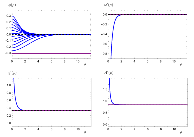
Figure 1: Background fields in illustrative examples of confining solutions with $\rho_{o}=0$. Left to right and top to bottom: the functions $\phi(\rho)$, $\omega^{\prime}(\rho)$, $\chi^{\prime}(\rho)$, and $A^{\prime}(\rho)$. For comparison, the horizontal lines represent the DW solutions at the $\phi_{UV}$ (black, dashing) and $\phi_{IR}$ (purple, continuous). In confining solutions, $\omega$, $\chi$, and $A$ diverge at the end of space, but $\phi$ is finite.

These solutions are called confining, because the shrinking of the circle parametrised by $\eta$ is completely smooth, and, upon lifting the theory to type IIA, it is possible to apply the standard prescription that allows to compute the expectation value of a rectangular Wilson loop in the boundary theory, from which one can obtain a static potential between probe quarks that reproduces the expected asymptotic linear dependence on the quark separation—see Appendix C and references therein. The $\phi=0$ solution is the background discussed by Witten in Ref. Witten:1998zw , and the generalisations to the full class discussed here have been presented in Refs. Elander:2013jqa and Elander:2020fmv .

We depict examples of both confining and DW solutions in Fig. 1. It is worth noticing that, while in the plot showing $\phi(\rho)$ is it clearly possible to distinguish each non-trivial solution, including the DW cases for the two critical choices $\phi(\rho)=\phi_{UV}$ and $\phi(\rho)=\phi_{IR}$, by contrast, on the scale of the plots for the functions $\omega^{\prime}(\rho)$, $\chi^{\prime}(\rho)$, and $A^{\prime}(\rho)$, the difference between the various confining solutions is too small to be resolved, and so is the difference in curvature between the two DW solutions.

4 Linearised fluctuations and mass spectra

We devote this section to the calculation of the mass spectra of bound states of the confining field theory, which the dictionary of gauge-gravity dualities identifies with the spectrum of fluctuations around the gravity background. We treat the fluctuations of metric and active scalars using the gauge-invariant formalism developed in Refs. Bianchi:2003ug ; Berg:2005pd ; Berg:2006xy ; Elander:2009bm ; Elander:2010wd (and Elander:2018aub ; Elander:2020csd ). For the $p$-forms, with $p=0,1,2$, we implement the $R_{\xi}$ gauge and focus only on physical combinations of the fluctuated fields that do not depend on the gauge-fixing ($\xi$) parameters, following the general principles enunciated in Ref. Elander:2018aub . Extended details about the treatment of the $3$-form, in particular in reference to the self-duality conditions, are shown in Appendix A. The technical details on how we perform the calculations are relegated to Appendix B, as well as details about the notation, where appropriate, while in this section we discuss only the physical results.

In order to perform the numerical calculations yielding the spectrum, we introduce a regulating procedure, and the extrapolation to the physical results is obtained by a process that resembles what in the lattice literature is referred to as improvement. We define two boundaries $\rho_{1}$ and $\rho_{2}$ to the holographic coordinate so that $\rho_{1}\leq\rho\leq\rho_{2}$, and add boundary-localised terms in the action, which determine the boundary conditions obeyed by the fluctuations. We then compute the spectrum of small fluctuations that obey such boundary conditions, identifying the discrete values of $M^{2}=-q^{2}$ (where $q^{\mu}$ is the four-momentum of the fluctuations) for which the system admits solutions. The physical spectrum is recovered in the limit $\rho_{1}\rightarrow\rho_{o}$ and $\rho_{2}\rightarrow+\infty$. We could perform the calculations explicitly for finite $\rho_{1}$ and $\rho_{2}$, and then repeat the calculations and extrapolate towards the physical limits, as was done for example in Ref. Elander:2020fmv . Instead of doing so, we apply the boundary conditions to the asymptotic expansions of the fluctuations—see Appendix B.3.1 and B.3.2—and then use what results in order to set up the boundary conditions in the numerical study. By doing so, the convergence of the spectra computed at finite cutoffs is much faster, and as we shall see we obtained improved results in respect to the literature. We notice in passing that for generic (non fine-tuned) choices of boundary terms this process selects the subleading behaviors in the solutions of the linearised equations, in agreement with standard procedures of the gauge-gravity dictionary. We will return to the case of special, fine-tuned choices, and their consequences, in Section 5.1.

When we look at the spectrum of states of the boundary theory, by studying the fluctuations around the background solutions, it is best to count states in terms of massive representations of the Poincaré group. We expect the following towers of four-dimensional composite states to emerge—see also Table 1.

• A tower of spin-2 massive tensors, from the graviton (5 dofs each).

• Three towers of scalars, related to gauge invariant combinations of the active scalars and the trace of the metric.

• Thirty inactive scalars giving rise to as many towers, with the degeneracies of the $SO(4)$ multiplets they belong to ($9\oplus 1\oplus 4\oplus 4\oplus 6\oplus 6$).

• Seventeen massive $1$-forms corresponding to towers of spin-1 states, with degeneracies dictated by the representations of $SO(4)$ ($1\oplus 1\oplus 4\oplus 6\oplus 4\oplus 1$). Eight of these towers are referred to as ‘vectors’ in the following, the other nine being dubbed ‘axial-vectors.’

• Nine towers of pseudoscalars, transforming as $4\oplus 4\oplus 1$ of $SO(4)$—hence reaching the total of $42$ scalars—closely associated with the nine aforementioned axial-vectors by the Higgs mechanism.

• Thirty dofs represented by the $2$-forms, yielding ten more towers of massive vectors ($3$ dofs each), transforming as $4\oplus 1\oplus 4\oplus 1$ of $SO(4)$.

The degeneracies due to $SO(4)$ representations imply that beside the tower of spin-2 states ($1$ sequence of mass eigenstates), there are $12$ sequences of masses corresponding to the spin-0 towers, and $10$ different sequences of masses for the spin-1 particles. In summary, the $128$ bosonic degrees of freedom organise themselves in representations of $SO(4)$ and of the Poincaré group to yield $23$ distinct sequences of mass eigenstates.

4.1 Tensor and active scalars

In this subsection, we consider the tower of states associated with the spin-2 massive graviton, and the three towers of scalars obtained by fluctuating the three active scalars $(\phi,\chi,\omega)$. The main results have already been presented elsewhere (see Ref. Elander:2020fmv and references therein), and this short section serves mostly to make the presentation self-contained, as well as to cross-check that the results be consistent with the literature.

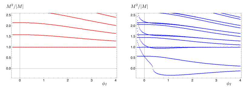
Figure 2: Mass spectrum $M^{2}=-q^{2}$ of tensor modes (left panel) and active scalars (right panel) as a function of the parameter $\phi_{I}$, normalised in units of the lightest tensor mode. Numerical calculations use $\rho_{1}=10^{-10}$ and $\rho_{2}=10$.

In Fig. 2 we display the mass spectrum of fluctuations of the metric and of the three active scalars. We summarise in the caption of Fig. 2 and in Appendix B, respectively, the details of the numerical and formal manipulations we implement to compute the mass spectrum. We notice that while the equations and boundary conditions for this sector of the spectrum are those in Ref. Elander:2020fmv , the process by means of which we implemented the boundary conditions improves the convergence in respect to Ref. Elander:2020fmv , better removing spurious cutoff artefacts, and hence the results on display in this paper are a numerical improvement upon the existing literature.

We normalise the spectra to the mass of the lightest tensor bound state, to remove spurious dependences on arbitrary additive integration constants in the background values of $A$, $\chi$ and $\omega$. The results are in agreement with the literature. In particular, we notice the emergence of a tachyonic state (with negative $M^{2}<0$), for backgrounds generated with large and positive values of $\phi_{I}$. We notice however that while the tachyon appears first at $\phi_{I}\lesssim 0.447$ in Ref. Elander:2020fmv , with the improvement we implement this is now happening at $\phi_{I}\sim 0.36$. In the region in which this state is light, it is also an approximate dilaton, as in Ref. Elander:2020fmv it is shown that its composition consists predominantly of the fluctuations of the trace of the metric (which holographically corresponds to the dilatation operator).

4.2 All other scalars

To the best of our knowledge, the rest of the spectrum has not been computed before for general $\phi_{I}$. In particular, we report here the first calculation of the spectrum of all the spin-0 states that descend from maximal supergravity.

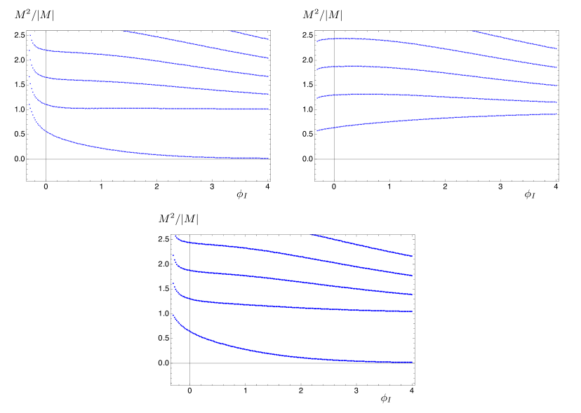
Figure 3: Mass spectrum, with $M^{2}=-q^{2}$, of the three groups of pseudoscalar modes and their excited states as a function of the parameter $\phi_{I}$, normalised in units of the lightest tensor mode. The markers are chosen to match the representations under $SO(4)$. Left to right and top to bottom: the fourth, fifth and sixth element of ${\cal H}^{(1)\,A}_{\,\,\,M}$ as in Eq. (85). Numerical calculations use $\rho_{1}=10^{-10}$ and $\rho_{2}=10$.

We start with the three towers of Goldstone bosons, and we report their mass spectra in Fig. 3. As anticipated, they transform as $4\oplus 4\oplus 1$ of $SO(4)$, respectively. The first of the towers describes the $SO(5)/SO(4)$ coset, and the lightest states of this sequence correspond to the pNGBs of the dual theory. They acquire a mass in the presence of explicit symmetry breaking in the dual theory. This is signalled by the presence of $\phi_{2}\neq 0$, in the UV expansion of the background solutions in Eq. (3.1). Interestingly, we notice that when $\phi_{I}$ is positive and large, this group of degenerate bound states becomes parametrically light. We know from Refs. Elander:2020fmv ; Roughley:2021suu that this is the limit in which $\phi_{4}$ is enhanced with respect to $\phi_{2}$. This is the limit in which one intuitively expects to see Goldstone bosons, and the continuous connection between the region of parameter space with large and small $\phi_{I}$ is the central element suggesting to interpret the lightest excitations in these towers of states as pNGBs—in spite of their large mass when $\phi=0$.

The other two towers ($5$ dofs) correspond to the breaking of the $SO(6)$ to $SO(5)$. This is somewhat counterintuitive and requires further explanation. We remind the Reader that $SO(6)$ is the global symmetry of the five-sphere $S^{5}$, and that maximal supergravity in five dimensions indeed has such gauged symmetry. We also remind the Reader that the field content of the ungauged theory is the same as that of the gauged theory. Because there is no $S^{5}$ in the geometry, the additional $5=4\oplus 1$ Goldstone bosons have no apparent reason to be light. Yet, interestingly, when $\phi_{I}$ is large and positive, the $SO(4)$ singlet becomes parametrically light. As a tangential remark, it may be worth reminding the Reader that $SO(6)/SO(5)\sim SU(4)/Sp(4)$ is another coset which has attracted some attention in the literature (see, e.g., Refs. Barnard:2013zea ; Arthur:2016ozw ; Pica:2016zst ; Drach:2017btk ; Drach:2020wux ; Bennett:2017kga ; Bennett:2019jzz ; Bennett:2019cxd ). While it might be interesting to study models based on this coset, this is clearly beyond the purposes of this paper, and requires a generalisation of the model proposed here.

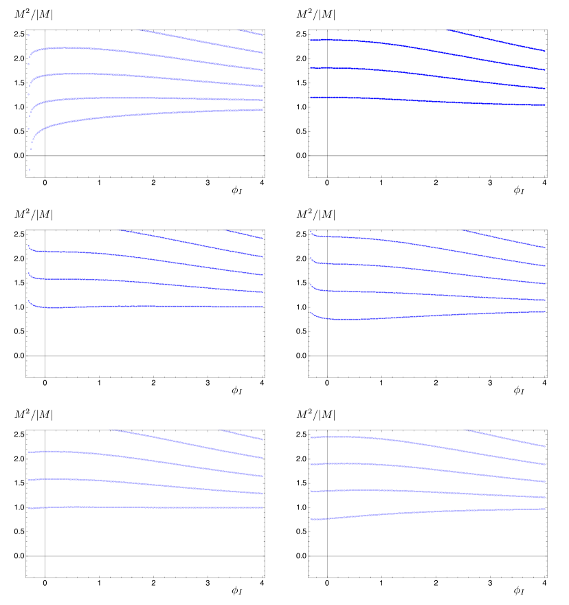
Figure 4: Mass spectrum, with $M^{2}=-q^{2}$, of fluctuations of the scalar fields that vanish on the backgrounds, as a function of the parameter $\phi_{I}$. The masses are expressed in units of the lightest tensor mode in the spectrum. The markers are chosen to match the representations under $SO(4)$. Left to right and top to bottom, the nine degenerate scalar modes denoted in the main body of the paper as $s^{\tilde{A}}$, the singlet $\omega_{6}$, the four degenerate $A_{6}^{\hat{A}}$, the four degenerate $A_{7}^{\hat{A}}$, the six degenerate $A_{6}^{\bar{A}}$ and the six degenerate $A_{7}^{\bar{A}}$. Numerical calculations use $\rho_{1}=10^{-10}$ and $\rho_{2}=10$.

In Fig. 4 we display the masses of the other scalar fluctuations. As has been known for quite a long time Pernici:1984zw , the non-supersymmetric critical point of the seven-dimensional potential is perturbatively unstable. The nine scalars $s^{\tilde{A}}$ have mass (in seven dimensions) below the unitarity bound, when evaluated as a fluctautation around the AdS₇ solution with $\langle\phi\rangle=\phi_{IR}$. In the case of this paper, some of the flows we are studying see the scalar $\phi$ approach this non-supersymmetric critical point, and hence there is a legitimate concern that tachyons might appear, in spite of the fact that the theory is dimensionally reduced, and confining solutions do not exhibit local five-dimensional Poincaré invariance. Direct calculation shows that there are indeed nine degenerate tachyons in the spectrum of the $s^{\tilde{A}}$ states, which appear for values of the parameter $\phi_{I}\lesssim-0.26$ close to $\phi_{IR}$. As in the case of the other dynamically-generated tachyon we discussed in Sec. 4.1 (among the fluctuations of the active scalars), we expect a phase transition to be present, to separate the tachyonic phase from the physical one. Contrary to the case of the active scalar for large and positive $\phi_{I}$, though, we know that this scalar is not a dilaton, as it is associated with fluctuations of a field that vanishes in the background, and hence these fluctuations cannot mix with the trace of the metric, which is the bulk field associated to the boundary dilatation operator—an extensive discussion of this general argument can be found in Ref. Elander:2020csd .

The other five groups of degenerate scalar fluctuations do not display any qualitative nor quantitative features that deserve further attention. The towers of states associated with the singlet $\omega_{6}$, the four degenerate $A_{6}^{\hat{A}}$, the four degenerate $A_{7}^{\hat{A}}$, the six degenerate $A_{6}^{\bar{A}}$ and the six degenerate $A_{7}^{\bar{A}}$, all have only mild dependence on $\phi_{I}$, and have masses that start around the same value of the spin-2 states, with the $6$ particles associated with $A_{6}^{\bar{A}}$ showing almost exact degeneracy with the tensors. We will not discuss these five sequences of masses any further in the following.

4.3 $1$-forms in five dimensions

Figure 5: Mass spectrum, with $M^{2}=-q^{2}$, of the (gauge-invariant) transverse fluctuations of the $1$-forms, as a function of the parameter $\phi_{I}$. The masses are normalised to the lightest tensor mode. The markers are chosen to match the representations under $SO(4)$. Left to right and top to bottom: $\chi_{\mu}$, $\omega_{\mu}$, the six $A^{\bar{A}}_{\mu}$ (all these states are also called vectors elsewhere), the four $A^{\hat{A}}_{\mu}$, the four $S_{67\mu\,\bar{\beta}}$, and $S_{67\mu\,5}$ (the axial-vectors). Numerical calculations use $\rho_{1}=10^{-10}$ and $\rho_{2}=10$.

Our numerical results for the six towers of excitations of the $1$-forms (vectors) are depicted in Fig. 5. Two things are worth noticing. First, the unexpected fact that the spin-1 states corresponding to the axial-vector fields $S_{67\mu\,\bar{\beta}}$ and $S_{67\mu\,5}$, which together transform as a $5$ of $SO(5)$, and span the $SO(6)/SO(5)$ coset, are not significantly heavier than the spin-1 states related to the gauged $SO(5)$. We would have expected the latter, comprising the vectors along the $SO(4)$, and the (axial-)vectors along the $SO(5)/SO(4)$ directions to be the lightest spin-1 states, somewhat separated from the others, as in generic QCD-like theories, in which, aside from the pNGBs, the lightest among the other bound states are the generalisations of the $\rho$ and $a_{1}$ mesons. Such separation is not there, and we will also find additional spin-1 states with comparable masses in the next subsection.

Second, for non-vanishing $\langle\phi\rangle$, the background breaks $SO(5)$ to $SO(4)$, and produces a splitting between the masses of the corresponding two groups of towers, as expected. But we find that the sign of the mass splitting depends on the sign of $\phi_{I}$. The six spin-1 states $A_{\mu}^{\bar{A}}$, broadly speaking corresponding to the $\rho$ mesons, are lighter than the four $A_{\mu}^{\hat{A}}$ for negative values of $\phi_{I}<0$. But when $\phi_{I}>0$, this ordering is inverted. This effect, if appearing in the absence of explicit breaking of the global symmetry, would be a possible signature of violations of unitarity, as it is not what expected from the analysis of dispersion relations in field theory. But the holographic interpretation of the backgrounds, in field-theoretical terms, indicates that we are in the presence of explicit symmetry breaking, and hence the sign of the splitting is a free parameter.

The other $1$-forms do not display features of particular physical interest. The fluctuations of $\chi_{\mu}$, $\omega_{\mu}$—or, better, their gauge-invariant, transverse components—all yield results in which even the lightest mass eigenvalue is no lighter than the strong coupling scale, which in this paper we conventionally associate with the mass of the lightest spin-2 tensor mode. The $S_{67O\,{\alpha}}$ fields are related by the self-duality conditions to the $S_{MNO\,\alpha}$ fields, and hence we do not need to study the equations of motion and boundary conditions obeyed by the latter, as they cannot yield additional information (for details, see Appendix A).

4.4 Massive $2$-forms in five dimensions

The treatment of the massive $2$-forms (in five dimensions) starts from the derivation of the equations of motion for $S_{6NO}$ and $S_{7NO}$, which is summarised in Appendix A, and yields four additional towers of spin-1 particles in the dual four-dimensional theory. Along the lines of thought we followed for the $1$-forms, we rewrite the five-dimensional action in a manifestly gauge-invariant form first, and then implement the $2$-form generalisation of the $R_{\xi}$ gauge, by following the formal treatment in Ref. Elander:2018aub . By doing so, we isolate the gauge-independent, transverse component—which we generically denote by $B_{\mu\nu}$ ($B^{\prime}_{\mu\nu}$) and $X_{\mu}$ ($X^{\prime}_{\mu}$)—and hence identify the physical spectrum of states without ambiguities. We summarise only the most important final results in Appendix B, in particular the implications of the fact that the $3$-forms obey a self-duality condition, which is necessary for consistency.

Figure 6: Mass spectrum, with $M^{2}=-q^{2}$, of the spin-1 particles coming from the $2$-forms in five dimensions, as a function of the parameter $\phi_{I}$, and normalised to the lightest tensor mode. The markers are chosen to match the representations under $SO(4)$. Left to right and top to bottom: the four $B_{\mu\nu\,\bar{\beta}}$, the four $X_{\mu\,\bar{\beta}}$, $B_{\mu\nu\,5}$, and $X_{\mu\,5}$. Numerical calculations use $\rho_{1}=10^{-10}$ and $\rho_{2}=10$.

As the resulting equations and boundary conditions are peculiarly affected by the self-duality conditions, we exhibit them explicitly in the body of the paper, while more detail is in Appendix B. They are the following:

$$0 = \left[\frac{}{}q^{2}e^{-2A}-\partial_{r}^{2}+\frac{\partial_{r}H^{(2)\prime}_{A}}{H^{(2)\prime}_{A}}\partial_{r}+m^{2}H^{(2)}_{A}H^{(2)\prime}_{A}\right]P^{\mu\rho}P^{\nu\sigma}B^{A}_{\,\,\,\rho\sigma}(q,r)\,,$$ (125)

$$0 = \left.\left[\frac{}{}\partial_{r}+\sqrt{H^{(2)}_{A}H^{(2)\prime}_{A}m^{2}}\right]P^{\mu\rho}P^{\nu\sigma}B^{A}_{\,\,\,\rho\sigma}(q,r)\right|_{r=r_{i}}\,,$$ (126)

$$0 = \left[\frac{}{}\partial_{r}^{2}-\frac{\partial_{r}H^{(2)}_{A}}{H^{(2)}_{A}}\partial_{r}-e^{-2A}q^{2}-m^{2}{H^{(2)}_{A}}H^{(2)\prime}_{A}\right]X^{A}_{\,\,\,\mu}(q,r)\,,$$ (127)

$$0 = \left.\frac{}{}\left[\frac{}{}\partial_{r}+\sqrt{H^{(2)}_{A}H^{(2)\prime}_{A}m^{2}}\right]X^{A}_{\,\,\,\mu}(q,r)\right|_{r=r_{i}}\,,$$ (128)

where $A=1\,,\cdots\,,5$, and these equations describe both the degrees of freedom contained in the $2$-forms denoted by $S_{6NO}$ and $S_{7NO}$. The functions $H^{(2)}_{A}$ and $H^{(2)\prime}_{A}=1/K^{(2)}_{A}$ are given in Eqs. (110–117). We use the identification of $B_{\mu\nu}$ (and $X_{\mu}$) with the gauge-invariant field containing $S_{6NO}$, purely as a conventional choice. As shown in Appendix B.2, the corresponding equations for $B^{\prime}_{\mu\nu}$ and $X^{\prime}_{\mu}$, associated with $S_{7NO}$, can be brought into the same form after a judicious choice of boundary conditions and the identification of $B^{\prime}_{\mu\nu}$ with $X_{\mu}$ and vice versa. This is made possible due to the self-dual nature of $S_{MNO}$, and hence the entirety of the associated part of the spectrum can be extracted by considering only the equations for $B_{\mu\nu}$ and $X_{\mu}$ given in Eqs. (125–128).

Once more, we impose these boundary conditions on the asymptotic expansions of the fluctuations, and then set up the numerical solver to match the resulting asymptotics, which effectively retains only the subleading terms in the expansions themselves. We display the results in Fig. 6. As one can see, all four sets of towers of states show the generic expectation that all these fields, which correspond to spin-1 composite states, are heavy, their masses being of the order of those of the spin-$2$ tensors or higher. With one valuable exception: the lightest mode corresponding to component $X_{\mu\,5}$, along the broken generator of $SO(5)$, becomes parametrically light, for asymptotically large values of $\phi_{I}$.

5 Towards composite Higgs models

Figure 7: Detail of the combined mass spectrum $M^{2}=-q^{2}$ of all the bosons, as a function of the parameter $\phi_{I}$, normalised to the lightest tensor mode, and restricted to the low-mass region. In red we depict the spin-2 particles, in black the spin-1, in blue the spin-0. The markers are chosen to match the representations under $SO(4)$, while the legend refers back to the notation in Table 1. Numerical calculations use $\rho_{1}=10^{-10}$ and $\rho_{2}=10$.

So far in this paper, we reported on the results of the calculation of the complete spectrum of excitations of the $128$ bosonic degrees of freedom of the theory. We start this section by presenting a summary plot of the physical results of our extensive study, which are displayed in Fig. 7.

The number of bosonic states is so large that the sequence of levels densely fills the positive values of the mass above that of the lightest spin-$2$ (tensor) state. We remark on the presence of a degeneracy between the spin-2 states with a tower of spin-1 and of spin-0 states, which (for $\phi_{I}=0$) had been observed before in the literature Brower:2000rp . In general terms, looking at heavy states with this formalism is not particularly interesting: in spite of retaining a significant number of supergravity fields, we are still neglecting the excitations that depend non-trivially on the coordinates on the two circles and on the four-sphere in the interior of the geometry, and furthermore all the possible other excitations that are not captured by supergravity. Yet, if we focus our attention on states that are appreciably lighter than the spin-$2$ tensors, some interesting patterns emerge, which do not depend on the aforementioned simplifications and approximations.

We remind the Reader of some of the results already discussed in previous sections. The first observation we make is that two mass eigenstates for spin-0 particles become tachyonic in (separate) parts of the parameter space. At negative $\phi_{I}$, large enough that the backgrounds approach the non-supersymmetric critical point with $\langle\phi\rangle=\phi_{IR}$, these tachyons correspond to the lightest excitations of the nine $s^{\tilde{A}}$, and their negative mass is a consequence of the instability of such critical point. Conversely, at large and positive values of $\phi_{I}$, the state that becomes tachyonic is a fluctuation of the background active scalars, and mixes with the trace of the metric, so that this tachyon is also a dilaton, at least approximately Elander:2020fmv .

There is a region of small to moderate values of $\phi_{I}$ over which such (perturbative) instabilities are absent. We do not know what is the current extent of such region: both at positive and negative $\phi_{I}$, a phase transition must be present, separating the stable, physical branch of confining solutions from the unstable ones. This problem was studied in Ref. Elander:2020fmv , which demonstated the existence of a first-order phase transition at a moderate value of $\phi_{I}>0$. This was supported by establishing the metastable nature of the gravity solutions in the region $0.04\lesssim\phi_{I}\lesssim 0.4$. No analogous study has, to the best of our knowledge, been performed for negative values of $\phi_{I}$, and we leave this open question for future investigations.

As expected, the aforementioned two scalar mass eigenstates become exactly degenerate for $\phi_{I}=0=\phi$, where they are both part of the $14$ of the enhanced $SO(5)$ symmetry. Interestingly, they are also close to degenerate with one of the lightest active states that corresponds to fluctuations of the fields $\{\omega,\chi\}$. It is also worth noticing that a second fluctuation of the active scalars becomes parameterically light when $\phi_{I}$ is taken to be large, so that in this limit two of the spin-0 $SO(4)$ singlets become massless.

One of the pseudo-scalar eigenstates, corresponding to the $4$ pNGBs of the $SO(5)\rightarrow SO(4)$ breaking, becomes massless for $\phi_{I}\rightarrow+\infty$. Interestingly, also one pseudoscalar $SO(4)$ singlet, and the degenerate spin-1 $SO(4)$ singlet, become massless in this limit. Asymptotically at large $\phi_{I}$, we find that the spectrum approaches that of a gapped continuum starting at the threshold set by the mass of the tensors, accompanied by a number of massless states corresponding to the aforementioned two scalars, five pseudo-scalars and one vector.

5.1 Boundary terms and pNGBs

We complete this section with an exercise that involves the boundary terms in the action. We focus on the boundary at $\rho_{2}$, and specifically on the boundary term for the four pseudo-scalars $\pi^{\hat{A}}$. No explicit mass terms are allowed for these fields, due to gauge invariance, but the combination $\partial_{\mu}\pi^{\hat{A}}+2mA_{\mu}^{\,\,\,\hat{A}}$ is gauge invariant, and hence a boundary-localised term quadratic in this combination is allowed. Its coefficient is denoted by $C_{2}$ in Eqs. (208) and (210) in the Appendix. We would like to assess how much the spectrum of the spin-0 and spin-1 states would be affected by fine-tuned choices of $C_{2}\neq 0$.

The reason why this is interesting relates to the connection with phenomenological CHMs. A non-zero $C_{2}$ might emerge from the coupling of the pNGBs to an external sector of the theory, as is envisioned in CHMs, for which this sector is the standard model of particle physics—the lightest excitations of the four $\pi^{\hat{A}}$ fields being related to the Higgs fields of the standard model. In CHMs, such couplings not only change the dynamics of the pseudoscalars, but must induce an instability, that ultimately triggers electroweak symmetry breaking—$SO(4)$ must break spontaneously to $SO(3)$ in the vacuum. Of course, a realistic model would require to also embed the $SU(2)_{L}\times U(1)_{Y}$ gauge group into the $SO(4)$ symmetry, which would require changing also the appropriate $D_{2}$ terms in Eqs. (208) and (210). But we leave this model-building task, together with other model-building considerations, as well as the whole programme of studying vacuum (mis-)alignment and of assessing the amount of fine-tuning, to future investigations. Here we just consider whether we can make the mass of the pNGBs parameterically small, and possibly negative, by dialing $C_{2}$, without further attention to phenomenological and model-building considerations.

To be more precise, let us reconsider the numerical procedure we adopted in the treatment of this particular multiplet of pseudoscalars. For $C_{2}=0$, Eq. (210), when taking the limit $\rho_{2}\rightarrow+\infty$, amounts to selecting the subleading fluctuation in the asymptotic expansion of $\mathfrak{p}^{1}$ in Eq. (B.3.1)—effectively restricting the fluctuations to have $\mathfrak{p}^{1}_{\,\,\,l}=0$. Explicitly, we see that this is the case by making use of the changes of variable $\partial_{r}=e^{-\chi}\partial_{\rho}$ and $z=e^{-\rho/2}$ to rewrite Eq. (210) as

$$0 = \left.\left[\frac{}{}C_{2}e^{-\chi(\rho)}\partial_{\rho}+G^{(1)}(\rho)\right]X(q,\rho)\right|_{\rho=\rho_{2}}$$ (129)

$$= \left.\left[-\frac{1}{2}C_{2}e^{-\chi(z)}z\partial_{z}+G^{(1)}(z)\right]X(q,z)\right|_{z=e^{-\rho_{2}/2}}$$

$$= \left.\left[-\frac{1}{2}C_{2}e^{-\chi(z)}\,\mathfrak{p}^{1}_{\,\,\,l}+G^{(1)}(z)\left(\mathfrak{p}^{1}_{\,\,\,0}+\log(z)\mathfrak{p}^{1}_{\,\,\,l}\right)+\cdots\right]\right|_{z=e^{-\rho_{2}/2}}\,,$$

where we made explicit use of the first line of Eq. (B.3.1), and where $G^{(1)}=\sinh^{2}\left(\sqrt{5}\phi/2\right)$ is the factor appearing in the fourth block of the diagonal matrix of Eq. (100). As the term with the explicit dependence on $\log(z)$ is dominant for $C_{2}=0$, by taking the limit $\rho_{2}\rightarrow+\infty$ we are effectively setting $\mathfrak{p}^{1}_{\,\,\,l}=0$.

This conclusion holds for any generic choice of $C_{2}$ such that $\lim\limits_{\rho_{2}\rightarrow\infty}\left(\frac{C_{2}(\rho_{2})e^{-\chi(\rho_{2})}}{G^{(1)}(\rho_{2})}+\rho_{2}\right)=\pm\infty$. The other extreme case appears if we allow $C_{2}$ to be a function of $\rho_{2}$, such that when we take $\rho_{2}\rightarrow+\infty$ we find that $\lim\limits_{\rho_{2}\rightarrow\infty}\left(\frac{C_{2}(\rho_{2})e^{-\chi(\rho_{2})}}{G^{(1)}(\rho_{2})}+\rho_{2}\right)=0$. In this case, we are fixing $\mathfrak{p}^{1}_{\,\,\,0}=0$. But we can make a fine-tuned choice, by making $C_{2}$ a function of $\rho_{2}$, and requiring that for a given $\rho_{2}$ we dial

$$-\frac{1}{2}C_{2}(\rho_{2})e^{-\chi(\rho_{2})} \equiv \frac{1}{2}G^{(1)}(\rho_{2})\times\left(\frac{}{}\rho_{2}+2c_{2}\right)\,,$$ (130)

with $c_{2}$ a constant. By doing so, the boundary condition reduces to

$$0 = \left.G^{(1)}(z)\left(\mathfrak{p}^{1}_{\,\,\,0}+c_{2}\,\mathfrak{p}^{1}_{\,\,\,l}\right)\right|_{z=e^{-\rho_{2}/2}}\,.$$ (131)

This process highlights the presence of an additional free parameter, $c_{2}$, in the theory, and this free parameter can be dialed to change the spectrum. Doing so requires fine-tuning, because the scaling of $C_{2}$ has no a priori relation with the bulk warp factors, such as $G^{(1)}(\rho)$ and $e^{-\chi}$, and hence this mechanism amounts to a somewhat contrived exact calcellation, in the $\rho_{2}\rightarrow+\infty$ limit, between bulk and boundary-localised physical effects.

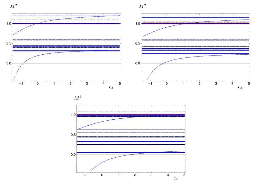
Figure 8: Detail of the combined mass spectrum $M^{2}=-q^{2}$ of all the bosons, for the choices of $\phi_{I}=-0.05,0.05,0.25$ (top-left, top-right, bottom panels), obtained by varying the parameter $c_{2}$ defined in Eq. (130). The colour and symbol coding is the same as in the earlier plots of the mass spectra. Numerical calculations use $\rho_{1}=10^{-10}$ and $\rho_{2}=10$.

We show in Fig. 8 the dependence of the spectrum, in particular for the four pNGBs, on $c_{2}$, for three representative values of $\phi_{I}$. The spectrum in Fig. 7 is recovered for $c_{2}\rightarrow+\infty$. In all cases, we notice the existence of a narrow range of $c_{2}$ for which the pseudoscalars are parametrically light, compared to the rest of the spectrum. This range appears in proximity of a fine-tuned choice of $c_{2}$ below which the pseudoscalar becomes anomalously light and tachyonic. Depending on the value of $\phi_{I}$, two different cases can be realised. For generic $\phi_{I}$ (represented here by $\phi_{I}=\pm 0.05$, as in the top panels of Fig. 8), by tuning $c_{2}$ one can realise a hierarchy between the mass of the pseudoscalars and the rest of the spectrum. The little hierarchy of scales that emerges in this way is suggestive of the case of interest in composite Higgs models: in order to trigger electroweak symmetry breaking one needs a choice of $c_{2}$ that makes the pseudoscalar tachyonic, and the instability would indicate that the vacuum might further break $SO(4)$ to a $SO(3)$ subgroup. Interestingly, this scenario is realised both for positive and negative values of $\phi_{I}$.

For larger and positive values of $\phi_{I}$, close to the appearance of a tachyon in the scalar spectrum, but for which the scalar mass squared is still positive, one can realise the scenario of composite Higgs models in which the low energy effective theory is the dilaton EFT. In this case one can envisage a low energy spectrum that contains also a pseudo-dilaton, together with the pNGBs. But to do so requires dialing to special values both $\phi_{I}$ and $c_{2}$. We defer the detailed realisation of a phenomenologically viable model of this type to future work.

Let us return to the rest of the bosonic spectrum. If, as suggested above, we modify $C_{2}$ for one of the pseudoscalar multiplets, the boundary term affects the associated axial-vector field as well, as the same parameter enters Eq. (208) as (210). For $D_{2}=0$, we find that the UV boundary condition is the following:

$$0 = \left.e^{2A(z)}\left[-\frac{1}{2}H^{(1)}(z)e^{-\chi(z)}z\partial_{z}+m^{2}C_{2}\right]P^{\mu\nu}A^{\hat{A}}_{\,\,\,\mu}(q,z)\right|_{z=e^{-\rho_{2}/2}}\,,$$ (132)

where $H^{(1)}(z)=\frac{1}{4}e^{\frac{3\phi}{\sqrt{5}}+2\chi}$ is the factor appearing in the fourth block of the diagonal matrix of Eq. (84). By replacing the aforementioned, fine-tuned choice of $C_{2}$, as well as the expansion in Eq. (242), we find

$$0 = \left[z\partial_{z}+\frac{2m^{2}e^{2\chi(z)}G^{(1)}(z)(\rho_{2}+2c_{2})}{H^{(1)}(z)}\right]\left[\frac{}{}\mathfrak{v}^{4}_{\,\,\,0}\left(1+z^{2}M^{2}+\cdots\right)+\mathfrak{v}^{4}_{\,\,\,4}z^{4}\right]\Big{|}_{z=e^{-\rho_{2}/2}}$$ (133)

$$= \left[z\partial_{z}+10\phi_{2}^{2}(\rho_{2}+2c_{2})z^{4}\right]\left[\frac{}{}\mathfrak{v}^{4}_{\,\,\,0}\left(1+z^{2}M^{2}+\cdots\right)+\mathfrak{v}^{4}_{\,\,\,4}z^{4}\right]\Big{|}_{z=e^{-\rho_{2}/2}}\,.$$

Even for the aforementioned, fine-tuned choices of $C_{2}$, these boundary conditions are equivalent, asymptotically, to setting the coefficient $\mathfrak{v}^{4}_{\,\,\,0}=0$ for the leading term emerging from the fluctuations, and hence this choice does not affect the spectrum of the axial vectors. In particular, all the 1-forms are massive, with $M^{2}\neq 0$.

6 Conclusions and Outlook

We reconsidered a holographic model of confining dynamics based upon a 1-parameter family of background solutions in maximal supergravity in seven dimensions, compactified on a 2-torus. The backgrounds are completely regular and smooth. The holographic calculation of the Wilson loop yields the static quark-antiquark potential expected in linear confinement. Furthermore, the 1-parameter family describes the breaking $SO(5)\rightarrow SO(4)$ of the global symmetry in the dual field theory. We presented two main, interrelated, sets of new results.

At first, we computed the spectrum of fluctuations of these models. The complete bosonic mass spectrum is interpreted in terms of bound states of the dual confining four-dimensional field theory. For the $SO(4)$ singlets, we improved the numerical treatment compared to earlier papers, and found agreement with other studies—when the results for the same states are available. One original part of this paper is that we extended the literature to include also states that are not singlets of the $SO(4)$ symmetry, and which had previously been ignored. We found that some of these multiplets are lighter than the singlets. We presented all the details of the calculations, from the decomposition of all the dimensionally reduced fields, to the treatment of the boundary conditions, taking special care to identify the physical, gauge-invariant degrees of freedom.

The second part of this study concerned the connection of this well established supergravity, and its background solutions, to the, superficially remote, CHM context. Having observed that the $SO(5)/SO(4)$ coset, characterising the field-theory dual of the present theory, also coincides with the one deployed in the construction of minimal CHMs, we focused attention on the mass spectrum of the four pNGBs associated with $SO(5)\rightarrow SO(4)$ breaking. In a complete CHM, the four fields providing the low-energy description of the pNGBs would become the four components of the Higgs doublet. As explained elsewhere (see for instance Ref. Agashe:2004rs , or reviews of CHMs such as Ref. Panico:2015jxa ), the coupling to the standard model fields, within the low energy dynamics, can trigger electroweak symmetry breaking, via vacuum misalignment. We restricted ourselves to consider a more limited question of principle. We showed how, by dialing specific boundary-localised terms, that are allowed by the symmetries and would be naturally generated by coupling the theory to an external weakly-coupled sector, it is indeed possible to realise a spectrum that resembles that of minimal CHMs, and ultimately trigger an instability, which appears at scales lower than that of the strong coupling dynamics. In passing, we also found that, for non-trivial parameter choices, the low energy spectrum may include also an approximate dilaton, besides the four pNGBs.

Within the language of gauge-gravity dualities, it is worth noticing that by dialing the two parameters denoted as $\phi_{I}$ and $c_{2}$ in the body of the paper, we gain the freedom to change the balance between explicit and spontaneous breaking of $SO(5)$. Let us try to make this statement more precise. Let us start from the case in which we do not include boundary localised terms, and in which $\phi_{I}=0$. The $SO(5)$ symmetry is exact, all of the spectrum is organised in $SO(5)$ multiplets, there are no pNGBs (see Appendix D). When we turn on $\phi_{I}\neq 0$, $SO(5)$ is broken in the background, and the analysis of the UV expansions shows the presence of both explicit and spontaneous breaking, via the coupling and vacuum expectation value of the operator dual to the field $\phi$. The parameter $\phi_{I}$ itself controls the balance of the two effects. In general, one can dial $\phi_{I}$ to large values, and hence recover a set of four parametrically light pNGBs in this extreme case. But this appears possible only at the price of exploring a region of parameter space where a tachyonic instability is present. In the non-tachyonic region of parameter space, the four pNGBs are not particularly light, their masses being just marginally smaller compared to other bosons.

The addition of the boundary-localised term (with finite $c_{2}$) allows to change the balance between explicit and spontaneous breaking. As a consequence of a cancellation between intrinsic breaking of $SO(5)$ in the strongly-coupled theory, and additional explicit breaking due to the weakly-coupled boundary effects, the mass spectrum displays light pNGBs. The result is not dissimilar from what emerges in other CHMs currently under investigation on the lattice and with EFT techniques—see the ample list of references in the introduction—in which the little hierarchy between the strong-coupling scale and the mass of the lightest scalars emerges in similar ways, from a cancellation requiring some moderate tuning.

Our results show that this very special theory provides a completion, in principle, for minimal CHMs. But let us qualify this statement. This theory provides quantitative information about the spectrum of states other than the pNGBs, such as the many scalars, spin-1 and spin-2 states we studied. Yet, to build a realistic model there are at least two major additional steps to take, before one can consider phenomenological implications and direct testability. First, one has to embed the $SU(2)\times U(1)$ symmetry of the standard model into $SO(4)$, and gauge it (weakly) by adding appropriate boundary-localised kinetic terms for the gauge bosons, in such a way that the dual field theory has a gauged, rather than global, symmetry. One then must study vacuum (mis-)alignment, and explicitly show that by dialling the appropriate boundary-localised term (generalising the aforementioned $c_{2}$ parameter to the realistic scenario) one can trigger electroweak symmetry breaking. After that, one can proceed to describe the full phenomenology of the resulting model, including the process of mass generation for the SM fermions, the study of the masses and couplings of the heavier states, and the calculation of precision observables both in the gauge and scalar sectors of the resulting CHM. The field content of the supergravity theory, and hence the bound states of its dual, includes towers of particles with non-trivial $SO(4)$ quantum numbers, and a calculable mass spectrum, making it potentially quite intriguing and well worth further investigation. This paper establishes the basic tools needed to start carrying out all these ambitious tasks in the near future.

Appendix A Of self-dual massive $3$-forms

In this Appendix, we match the action of the self-dual massive $3$-forms in seven dimensions to the action of massive $1$-forms and $2$-forms that we study in the body of the paper. Let us start from restricting our attention to the quadratic part of the action for the $3$-forms, borrowed from Eq. (2.2):

$${\cal S}_{7}^{(2)} = \int\mbox{d}^{7}x\left\{\sqrt{-\hat{g}_{7}}\left[-\frac{m^{2}}{4}\hat{g}^{\hat{M}\hat{P}}\hat{g}^{\hat{N}\hat{Q}}\hat{g}^{\hat{O}\hat{R}}\,\left(\frac{}{}e^{\frac{1}{\sqrt{5}}\phi}S_{\hat{M}\hat{N}\hat{O}\,\bar{\alpha}}\delta^{\bar{\alpha}\bar{\beta}}S_{\hat{P}\hat{Q}\hat{R}\,\bar{\beta}}+\right.\right.\right.$$

$$\left.\left.\left.+e^{-\frac{4}{\sqrt{5}}\phi}S_{\hat{M}\hat{N}\hat{O}\,5}S_{\hat{P}\hat{Q}\hat{R}\,5}\right)\right]+\frac{m}{24}\epsilon^{\hat{M}\hat{N}\hat{O}\hat{P}\hat{Q}\hat{R}\hat{S}}S_{\hat{M}\hat{N}\hat{O}\,\alpha}\delta^{\alpha\beta}\partial_{\hat{P}}S_{\hat{Q}\hat{R}\hat{S}\,\beta}\right\}\,.$$

Taking the variation of the action with respect to the fields, one obtains the equations of motion:

$$0 = -\frac{m^{2}}{2}\sqrt{-\hat{g}_{7}}\,\hat{g}^{\hat{M}\hat{P}}\hat{g}^{\hat{N}\hat{Q}}\hat{g}^{\hat{O}\hat{R}}\,e^{\frac{1}{\sqrt{5}}\phi}S_{\hat{P}\hat{Q}\hat{R}\,\bar{\beta}}+\frac{m}{12}\epsilon^{\hat{M}\hat{N}\hat{O}\hat{P}\hat{Q}\hat{R}\hat{S}}\partial_{\hat{P}}S_{\hat{Q}\hat{R}\hat{S}\,\bar{\beta}}\,,$$ (135)

$$0 = -\frac{m^{2}}{2}\sqrt{-\hat{g}_{7}}\,\hat{g}^{\hat{M}\hat{P}}\hat{g}^{\hat{N}\hat{Q}}\hat{g}^{\hat{O}\hat{R}}\,e^{-\frac{4}{\sqrt{5}}\phi}S_{\hat{P}\hat{Q}\hat{R}\,5}+\frac{m}{12}\epsilon^{\hat{M}\hat{N}\hat{O}\hat{P}\hat{Q}\hat{R}\hat{S}}\partial_{\hat{P}}S_{\hat{Q}\hat{R}\hat{S}\,5}\,,$$ (136)

where we separated the $SO(4)$ multiplet from the singlet, as they have different $\phi$-dependent mass terms. These equations implement the self-duality conditions that are necessary for massive $3$-forms to propagate $10$ degrees of freedom on-shell (and not $20$). The bulk equations are of first order, and relate the forms to their first derivative.

We reduce the equations to five dimensions with the ansatz for the metric in Eq. (20). The derivatives with respect to $\eta$ and $\zeta$ vanish for all the fields. We decompose the $3$-forms in their $S_{MNO}$ $S_{67O}$, $S_{6NO}$, and $S_{7NO}$ components, and make use of the fact that $\sqrt{-\hat{g}_{7}}=e^{-2\chi}\sqrt{-g_{5}}$, as well as that the indexes of the antisymmetric Levi-Civita symbols $\epsilon^{\hat{M}\hat{N}\hat{O}\hat{P}\hat{Q}\hat{R}\hat{S}}$ and $\epsilon^{MNOPQ}$ are lowered using the metrics in $D=7$ and $D=5$ dimensions, respectively. This exercise yields the following system of first-order coupled equations:

$$S_{67M\,\bar{\beta}} = \frac{1}{6m}\frac{e^{6\chi-\frac{1}{\sqrt{5}}\phi}}{\sqrt{-g_{5}}}\epsilon_{M}^{\ \ NOPQ}\partial_{N}S_{OPQ\,\bar{\beta}}\,,$$ (137)

$$S_{6MN\,\bar{\beta}} = -\frac{1}{2m}\frac{e^{\chi-2\omega-\frac{1}{\sqrt{5}}\phi}}{\sqrt{-g_{5}}}\epsilon_{MN}^{\ \ \ \ \,OPQ}\partial_{O}S_{7PQ\,\bar{\beta}}\,,$$ (138)

$$S_{7MN\,\bar{\beta}} = \frac{1}{2m}\frac{e^{\chi+2\omega-\frac{1}{\sqrt{5}}\phi}}{\sqrt{-g_{5}}}\epsilon_{MN}^{\ \ \ \ \,OPQ}\partial_{O}S_{6PQ\,\bar{\beta}}\,,$$ (139)

$$S_{{MNO}\,\bar{\beta}} = \frac{1}{m}\frac{e^{-4\chi-\frac{1}{\sqrt{5}}\phi}}{\sqrt{-g_{5}}}\epsilon_{MNO}^{\ \ \ \ \ \ \,PQ}\partial_{P}S_{67Q\,\bar{\beta}}\,,$$ (140)

$$S_{67M\,5} = \frac{1}{6m}\frac{e^{6\chi+\frac{4}{\sqrt{5}}\phi}}{\sqrt{-g_{5}}}\epsilon_{M}^{\ \ NOPQ}\partial_{N}S_{OPQ\,5}\,,$$ (141)

$$S_{6MN\,5} = -\frac{1}{2m}\frac{e^{\chi-2\omega+\frac{4}{\sqrt{5}}\phi}}{\sqrt{-g_{5}}}\epsilon_{MN}^{\ \ \ \ \,OPQ}\partial_{O}S_{7PQ\,5}\,,$$ (142)

$$S_{7MN\,5} = \frac{1}{2m}\frac{e^{\chi+2\omega+\frac{4}{\sqrt{5}}\phi}}{\sqrt{-g_{5}}}\epsilon_{MN}^{\ \ \ \ \,OPQ}\partial_{O}S_{6PQ\,5}\,,$$ (143)

$$S_{{MNO}\,5} = \frac{1}{m}\frac{e^{-4\chi+\frac{4}{\sqrt{5}}\phi}}{\sqrt{-g_{5}}}\epsilon_{MNO}^{\ \ \ \ \ \ \,PQ}\partial_{P}S_{67Q\,5}\,,$$ (144)

We can decouple the system into second-order equations, by resolving the mixing of $S_{67M}$ with $S_{MNO}$, and of $S_{6MN}$ with $S_{7MN}$. A substantial amount of algebra relies on the use of the following relations, that hold in five dimensions:

$$\epsilon^{SMNOP}\epsilon_{SM^{\prime}N^{\prime}O^{\prime}P^{\prime}} = (1!4!)g_{5}\frac{1}{4!}\left(\delta^{M}_{\,\,\,M^{\prime}}\delta^{N}_{\,\,\,N^{\prime}}\delta^{O}_{\,\,\,O^{\prime}}\delta^{P}_{\,\,\,P^{\prime}}-\delta^{M}_{\,\,\,M^{\prime}}\delta^{N}_{\,\,\,N^{\prime}}\delta^{O}_{\,\,\,P^{\prime}}\delta^{P}_{\,\,\,O^{\prime}}+\cdots\right),$$ (145)

$$\epsilon^{RSNOP}\epsilon_{RSN^{\prime}O^{\prime}P^{\prime}} = (2!3!)g_{5}\frac{1}{3!}\left(\delta^{N}_{\,\,\,N^{\prime}}\delta^{O}_{\,\,\,O^{\prime}}\delta^{P}_{\,\,\,P^{\prime}}-\delta^{N}_{\,\,\,N^{\prime}}\delta^{O}_{\,\,\,P^{\prime}}\delta^{P}_{\,\,\,O^{\prime}}+\cdots\right),$$ (146)

$$\epsilon^{QRSOP}\epsilon_{QRSO^{\prime}P^{\prime}} = (3!2!)g_{5}\frac{1}{2!}\left(\delta^{O}_{\,\,\,O^{\prime}}\delta^{P}_{\,\,\,P^{\prime}}-\delta^{O}_{\,\,\,P^{\prime}}\delta^{P}_{\,\,\,O^{\prime}}\right).$$ (147)

We also write $[n_{1}n_{2}\cdots n_{p}]\equiv\frac{1}{p!}(n_{1}n_{2}\cdots n_{p}-n_{2}n_{1}\cdots n_{p}+\cdots)$ to denote complete anti-symmetrisation. The equations of motion are hence written in terms of the tensors $S_{67O}$, $S_{6NO}$, formulated in the five-dimensional language, and they read as follows:

$$\frac{m^{2}\sqrt{-g_{5}}}{e^{6\chi-\frac{1}{\sqrt{5}}\phi}}{S}_{67}{}^{O\,\bar{\beta}} = 2\partial_{P}\left(\frac{\sqrt{-g_{5}}}{e^{4\chi+\frac{1}{\sqrt{5}}\phi}}\partial^{[P}{S}_{67}{}^{O]\,\bar{\beta}}\right)\,,$$ (148)

$$\frac{m^{2}\sqrt{-g_{5}}}{e^{\chi-2\omega-\frac{1}{\sqrt{5}}\phi}}{S}_{6}{}^{NO\,\bar{\beta}} = 3\partial_{P}\left(\frac{\sqrt{-g_{5}}}{e^{-\chi-2\omega+\frac{1}{\sqrt{5}}\phi}}{\partial}^{[P}{S}_{6}{}^{NO]\,\bar{\beta}}\right)\,,$$ (149)

$$\frac{m^{2}\sqrt{-g_{5}}}{e^{6\chi+\frac{4}{\sqrt{5}}\phi}}{S}_{67}{}^{O\,5} = 2\partial_{P}\left(\frac{\sqrt{-g_{5}}}{e^{4\chi-\frac{4}{\sqrt{5}}\phi}}\partial^{[P}{S}_{67}{}^{O]\,5}\right)\,,$$ (150)

$$\frac{m^{2}\sqrt{-g_{5}}}{e^{\chi-2\omega+\frac{4}{\sqrt{5}}\phi}}{S}_{6}{}^{NO\,5} = 3\partial_{P}\left(\frac{\sqrt{-g_{5}}}{e^{-\chi-2\omega-\frac{4}{\sqrt{5}}\phi}}{\partial}^{[P}{S}_{6}{}^{NO]\,5}\right)\,.$$ (151)

The equations for $S_{7NO}$ lead to the same states, ultimately as a consequence of the self-duality conditions, and we could omit them. They read as follows:

$$\frac{m^{2}\sqrt{-g_{5}}}{e^{\chi+2\omega-\frac{1}{\sqrt{5}}\phi}}{S}_{7}{}^{NO\,\bar{\beta}} = 3\partial_{P}\left(\frac{\sqrt{-g_{5}}}{e^{-\chi+2\omega+\frac{1}{\sqrt{5}}\phi}}{\partial}^{[P}{S}_{7}{}^{NO]\,\bar{\beta}}\right)\,,$$ (152)

$$\frac{m^{2}\sqrt{-g_{5}}}{e^{\chi+2\omega+\frac{4}{\sqrt{5}}\phi}}{S}_{7}{}^{NO\,5} = 3\partial_{P}\left(\frac{\sqrt{-g_{5}}}{e^{-\chi+2\omega-\frac{4}{\sqrt{5}}\phi}}{\partial}^{[P}{S}_{7}{}^{NO]\,5}\right)\,,$$ (153)

where we highlight the the dependence on $\omega$. For completeness, we report also the equations for the $S_{MNO\,\alpha}$ fields, although we do not use them anywhere in the paper:

$$\frac{{m^{2}}\sqrt{-g_{5}}}{e^{-4\chi-\frac{1}{\sqrt{5}}\phi}}S^{{MNO}\,\bar{\beta}} = 4\partial_{P}\left(\frac{\sqrt{-g_{5}}}{e^{-6\chi+\frac{1}{\sqrt{5}}\phi}}\partial^{[P}S^{MNO]\,\bar{\beta}}\right)\,,$$ (154)

$$\frac{{m^{2}}\sqrt{-g_{5}}}{e^{-4\chi+\frac{4}{\sqrt{5}}\phi}}S^{{MNO}\,5} = 4\partial_{{P}}\left(\frac{\sqrt{-g_{5}}}{e^{-6\chi-\frac{4}{\sqrt{5}}\phi}}\partial^{[P}S^{MNO]\,5}\right)\,.$$ (155)

For the next steps, we borrow the conventions from Eq. (B.48) of Ref. Elander:2018aub :

$${\cal S}_{5}^{(2)} = \int\mbox{d}^{5}x\sqrt{-g_{5}}\left\{-\frac{1}{4}H^{(2)}{\cal H}^{(2)}_{MN}{\cal H}^{(2)\,MN}\,-\frac{1}{12}\,K^{(2)}\,{\cal H}^{(3)}_{MNO}{\cal H}^{(3)\,MNO}\right\}\,,$$ (156)

where the gauge-invariant combinations are defined as follows:

$${\cal H}^{(2)}_{MN} = {\cal F}_{MN}+mB_{MN}\,,$$ (157)

$${\cal F}_{MN} = 2\partial_{[M}{\cal A}_{N]}\,,$$ (158)

$${\cal H}^{(3)}_{MNO} = 3\partial_{[M}B_{NO]}\,.$$ (159)

For the $1$-form we follow the notation in Eq. (B.27) of Ref. Elander:2018aub :

$${\cal S}_{5}^{(1)} = \int\mbox{d}^{5}x\sqrt{g_{5}}\left\{-\frac{1}{4}H^{(1)}F_{MN}F^{MN}+\right.$$

$$\left.-\frac{1}{2}G^{(1)}(\partial_{M}\pi+mA_{M})(\partial^{M}\pi+mA^{M})\right\}\,,$$

with $F_{MN}=2\partial_{[M}A_{N]}$. In both cases, the Lagrangian possessed a gauge symmetry, and we can set ${\cal A}_{M}=0=\pi$, in what we may call the unitary gauge. In this gauge, the equations of motion for the $2$-forms derived from Eq. (156) take the form:

$$m^{2}H^{(2)}\sqrt{-g_{5}}\,B^{NO} = 3\partial_{M}\left(K^{(2)}\sqrt{-g_{5}}\,\partial^{[M}B^{NO]}\right)\,,$$ (161)

and the equations of motion for the $1$-forms, derived from Eq. (A), take the form:

$$m^{2}G^{(1)}\sqrt{-g_{5}}\,A^{N} = 2\partial_{M}\left(H^{(1)}\sqrt{-g_{5}}\,\partial^{[M}A^{N]}\right)\,.$$ (162)

We introduce now the 2-forms $B_{MN}$ and $B_{MN}^{\prime}$ associated with $S_{6MN}$ and $S_{7MN}$, respectively, and the $1$-form $A_{M}$ associated with $S_{67M}$. By direct comparison between the two sets of equations of motion, we find that we can cast the action of the massive $2$-forms and $1$-forms originating in seven dimensions as in Eqs. (156) and (A), with the identification with five $2$-forms and five $1$-forms written as matrices in $SO(5)$ space:

$$B_{MN\,\alpha} = \left\{S_{6MN\,\bar{\beta}}\,,S_{6MN\,5}\right\}\,,$$ (163)

$$H^{(2)} = {\rm diag}\,\left(e^{-\chi+2\omega+\frac{1}{\sqrt{5}}\phi}\,,e^{-\chi+2\omega-\frac{4}{\sqrt{5}}\phi}\right)\,,$$ (164)

$$K^{(2)} = {\rm diag}\,\left(e^{\chi+2\omega-\frac{1}{\sqrt{5}}\phi}\,,e^{\chi+2\omega+\frac{4}{\sqrt{5}}\phi}\right)\,,$$ (165)

$$B^{\prime}_{MN\,\alpha} = \left\{S_{7MN\,\bar{\beta}}\,,S_{7MN\,5}\right\}\frac{}{}\,,$$ (166)

$$H^{(2)\prime} = {\rm diag}\,\left(e^{-\chi-2\omega+\frac{1}{\sqrt{5}}\phi}\,,e^{-\chi-2\omega-\frac{4}{\sqrt{5}}\phi}\right)\,=\,\left(K^{(2)}\right)^{-1}\,,$$ (167)

$$K^{(2)\prime} = {\rm diag}\,\left(e^{\chi-2\omega-\frac{1}{\sqrt{5}}\phi}\,,e^{\chi-2\omega+\frac{4}{\sqrt{5}}\phi}\right)\,=\,\left(H^{(2)}\right)^{-1}\,,$$ (168)

$$A_{M\,\alpha} = \left\{S_{67M\,\bar{\beta}}\,,S_{67M\,5}\right\}\,,$$ (169)

$$G^{(1)} = {\rm diag}\,\left(e^{-6\chi+\frac{1}{\sqrt{5}}\phi}\,,e^{-6\chi-\frac{4}{\sqrt{5}}\phi}\right)\,,$$ (170)

$$H^{(1)} = {\rm diag}\,\left(e^{-4\chi-\frac{1}{\sqrt{5}}\phi}\,,e^{-4\chi+\frac{4}{\sqrt{5}}\phi}\right)\,.$$ (171)

These identifications have been used to arrive to the relevant entries of the matrices in Eqs. (84), (100), (110), and (117).

Appendix B Formalism in five dimensions

We write here some general intermediate results, of a technical nature, that we use in the body of the paper for the definition of the background equations and the study of the spectrum of fluctuations, starting from the action written in the form of Eq. (3). We follow closely the notation adopted in Ref. Elander:2018aub , and indeed some parts of this Appendix are repetitious in this respect. Nevertheless, we find it useful to add this Appendix in order for the paper to be self-contained, and also to clarify possible ambiguities in the notation.

We start by repeating Eq. (3), and then devote the two subsequent subsections to the analysis of the system of active scalars coupled to gravity, and of the $p$-forms, respectively. We include an extensive discussion of the boundary conditions for the $2$-forms, as the self-duality condition affects them in a way that was not considered in Ref. Elander:2018aub . This section is concluded by displaying the asymptotic expansions for the fluctuations, which are used to impose the boundary conditions.

The action in Eq. (3) is the following:

$${\cal S}_{5} = \int\mbox{d}^{5}x\sqrt{-g_{5}}\left\{\frac{{R}}{4}-\frac{1}{2}g^{MN}G_{ab}\partial_{M}\Phi^{a}\partial_{N}\Phi^{b}-{\cal V}_{5}(\Phi^{a})+\right.$$

$$\left.-\frac{1}{2}g^{MN}G^{(0)}_{ab}\partial_{M}\Phi^{(0)a}\partial_{N}\Phi^{(0)b}-\frac{1}{2}m^{(0)2}_{ab}\Phi^{(0)a}\Phi^{(0)b}+\right.$$

$$\left.-\frac{1}{2}g^{MN}G^{(1)}_{AB}{\cal H}_{\ \ \ \ M}^{(1)A}{\cal H}^{(1)B}_{\ \ \ \ N}-\frac{1}{4}g^{MO}g^{NP}H^{(1)}_{AB}F_{\,\,\,\,MN}^{A}F^{B}_{\,\,\,\,OP}+\right.$$

$$\left.-\frac{1}{4}g^{MO}g^{NP}H^{(2)}_{\Gamma\Delta}{\cal H}^{(2)\Gamma}_{\,\,\,\,\,\,\,\,\,\,MN}{\cal H}^{(2)\Delta}_{\,\,\,\,\,\,\,\,\,\,\,OP}\,-\frac{1}{12}g^{MP}g^{NQ}g^{OR}K^{(2)}_{\Gamma\Delta}\,{\cal H}^{(3)\Gamma}_{\,\,\,\,\,\,\,\,\,\,MNO}{\cal H}^{(3)\Delta}_{\,\,\,\,\,\,\,\,\,\,\,PQR}\right\}\,.$$

The first line of the action depends on fields that may have non-trivial profiles in the vacuum, and their fluctuations are treated with the gauge-invariant sigma-model formalism. The subsequent three lines in the action contain the kinetic and mass terms for $p$-forms (with $p=0,1,2$), all of which have vanishing background profile.

B.1 Scalars coupled to gravity

It is convenient to make use of the gauge-invariant formalism developed in Refs. Bianchi:2003ug ; Berg:2005pd ; Berg:2006xy ; Elander:2009bm ; Elander:2010wd (and Elander:2018aub ; Elander:2020csd ). Borrowing from Refs. Berg:2005pd ; Elander:2010wd , consider $n$ real scalars $\Phi^{a}$, with $a=1\,,\,\cdots\,,\,n$ ($n=3$ in this paper). The action ${\cal S}_{D}$ of the sigma-model coupled to gravity in $D$ dimensions is written as follows:

$${\cal S}_{D} = \int\mbox{d}^{D}x\sqrt{-g}\left[\frac{{R}}{4}-\frac{1}{2}G_{ab}g^{MN}\partial_{M}\Phi^{a}\partial_{N}\Phi^{b}-{\mathcal{V}}(\Phi^{a})\right]\,.$$ (173)

The backgrounds of interest are identified by first introducing the following ansatz for the metric and scalars

$$\mbox{d}s^{2}_{D} = \mbox{d}r^{2}+e^{2{A}(r)}\,\eta_{\mu\nu}\mbox{d}x^{\mu}\mbox{d}x^{\nu}\,,$$ (174)

$$\Phi^{a} = \Phi^{a}(r)\,,$$ (175)

which assumes that all the background functions depend only on the radial direction $r$ in the geometry. Greek indexes $\mu,\nu$ extend over $D-1$ dimensions. The metric has signature mostly $+$. The connection symbols, with our conventions, are

$$\Gamma^{P}_{\,\,\,\,MN} \equiv \frac{1}{2}g^{PQ}\left(\frac{}{}\partial_{M}g_{NQ}+\partial_{N}g_{QM}-\partial_{Q}g_{MN}\right)\,,$$ (176)

while the Riemann tensor is

$$R_{MNP}^{\,\,\,\,\,\,\,\,\,\,\,\,\,\,\,\,\,Q} \equiv \partial_{N}\Gamma^{Q}_{\,\,\,\,MP}-\partial_{M}\Gamma^{Q}_{\,\,\,\,NP}+\Gamma^{S}_{\,\,\,\,MP}\Gamma^{Q}_{\,\,\,\,SN}-\Gamma^{S}_{\,\,\,\,NP}\Gamma^{Q}_{\,\,\,\,SM}\,,$$ (177)

the Ricci tensor is

$$R_{MN} \equiv R_{MPN}^{\,\,\,\,\,\,\,\,\,\,\,\,\,\,\,\,\,P}\,,$$ (178)

and finally the Ricci scalar is

$${R} \equiv R_{MN}g^{MN}\,.$$ (179)

The (gravity) covariant derivative for a $(1,1)$-tensor takes the form

$$\nabla_{M}T^{P}_{\,\,\,\,N} \equiv \partial_{M}T^{P}_{\,\,\,\,N}+\Gamma^{P}_{\,\,\,\,MQ}T^{Q}_{\,\,\,\,N}-\Gamma^{Q}_{\,\,\,\,MN}T^{P}_{\,\,\,\,Q}\,,$$ (180)

and generalises to any $(m,n)$-tensors.

The radial direction is bounded, with $r_{1}\leq r\leq r_{2}$, hence we also add boundary-localised terms to the action, which take the form

$${\cal S}_{1} = -\int\mbox{d}^{D}x\sqrt{-\tilde{g}}\delta(r-r_{1})\left[\frac{1}{2}K+\lambda_{(1)}(\Phi^{a})\right]\,,$$ (181)

$${\cal S}_{2} = \int\mbox{d}^{D}x\sqrt{-\tilde{g}}\delta(r-r_{2})\left[\frac{1}{2}K+\lambda_{(2)}(\Phi^{a})\right]\,,$$ (182)

where $K=g^{MN}K_{MN}$ is the extrinsic curvature and $\lambda_{(i)}$ are boundary-localised potentials. The signs of the two boundary-localised contributions to the action reflect the orientation of the ortho-normalised vector $N^{M}$, which is parallel to the radial direction $r$, and satisfies

$$g^{MN}N_{N}N_{M} = 1\,,$$ (183)

$$\tilde{g}_{MN}N^{N} = 0\,,$$ (184)

where $\tilde{g}_{MN}\equiv g_{MN}-N_{M}N_{N}$ is the induced metric. The second fundamental form is defined in terms of the covariant derivative $\nabla_{M}$, as $K_{MN}\equiv\nabla_{M}N_{M}$.

The sigma-model connection is defined in a similar fashion to gravity. It descends from the sigma-model metric $G_{ab}$ and the sigma-model derivative $\partial_{b}=\frac{\partial}{\partial\Phi^{b}}$, to read

$${\cal G}^{d}_{\,\,\,\,ab} \equiv \frac{1}{2}G^{dc}\left(\frac{}{}\partial_{a}G_{cb}+\partial_{b}G_{ca}-\partial_{c}G_{ab}\right)\,.$$ (185)

The sigma-model Riemann tensor is the following

$${\cal R}^{a}_{\,\,\,\,bcd} \equiv \partial_{c}{\cal G}^{a}_{\,\,\,\,bd}-\partial_{d}{\cal G}^{a}_{\,\,\,\,bc}+{\cal G}^{e}_{\,\,\,\,bd}{\cal G}^{a}_{\,\,\,\,ce}-{\cal G}^{e}_{\,\,\,\,bc}{\cal G}^{a}_{\,\,\,\,de}\,.$$ (186)

(The indexes in the conventions for the two Riemann tensors follow a reverse ordering.) Finally, the sigma-model covariant derivative is

$$D_{b}X^{d}_{\,\,\,\,a} \equiv \partial_{b}X^{d}_{\,\,\,\,a}+{\cal G}^{d}_{\,\,\,\,cb}X^{c}_{\,\,\,\,a}-{\cal G}^{c}_{\,\,\,\,ab}X^{d}_{\,\,\,\,c}\,.$$ (187)

The equations of motion satisfied by the background scalars are the following:

$$\partial_{r}^{2}\Phi^{a}\,+\,(D-1)\partial_{r}{A}\partial_{r}\Phi^{a}\,+\,{\cal G}^{a}_{\,\,\,\,bc}\partial_{r}\Phi^{b}\partial_{r}\Phi^{c}\,-\,\mathcal{V}^{a} = 0\,,$$ (188)

where the sigma-model derivatives are given by $\mathcal{V}^{a}\equiv G^{ab}\partial_{b}\mathcal{V}$, and $\partial_{b}\mathcal{V}\equiv\frac{\partial\mathcal{V}}{\partial\Phi^{b}}$. The Einstein equations reduce to

$$(D-1)(\partial_{r}{A})^{2}\,+\,\partial_{r}^{2}{A}\,+\,\frac{4}{D-2}\mathcal{V} = 0\,,$$ (189)

$$(D-1)(D-2)(\partial_{r}{A})^{2}\,-\,2G_{ab}\partial_{r}\Phi^{a}\partial_{r}\Phi^{b}\,+\,4\mathcal{V} = 0\,.$$ (190)

If the potential ${\mathcal{V}}$ can be written in terms of a superpotential $\cal W$ satisfying the following relation:

$${\mathcal{V}} = \frac{1}{2}G^{ab}\partial_{a}{\cal W}\partial_{b}{\cal W}-\frac{D-1}{D-2}{\cal W}^{2}\,,$$ (191)

then any solution of the first order system defined by

$$\partial_{r}{A} = -\frac{2}{D-2}{\cal W}\,,$$ (192)

$$\partial_{r}\Phi^{a} = G^{ab}\partial_{b}{\cal W}\,,$$ (193)

is also a solution of the equations of motion.

B.1.1 Fluctuations: tensors and active scalars

The fluctuations around the classical background of the active scalars and gravity are treated with the gauge-invariant formalism in Refs. Bianchi:2003ug ; Berg:2006xy ; Berg:2005pd ; Elander:2009bm ; Elander:2010wd . The scalar fields can be written as

$$\Phi^{a}(x^{\mu},r)=\Phi^{a}(r)+\varphi^{a}(x^{\mu},r)\,,$$ (194)

where $\varphi^{a}(x^{\mu},r)$ are small fluctuations around the background solutions $\Phi^{a}(r)$. By decomposing the metric according to the ADM formalism, one writes

$$\mbox{d}s_{D}^{2} = \left((1+\nu)^{2}+\nu_{\sigma}\nu^{\sigma}\right)\mbox{d}r^{2}+2\nu_{\mu}\mbox{d}x^{\mu}\mbox{d}r+e^{2{A}(r)}\left(\eta_{\mu\nu}+h_{\mu\nu}\right)\mbox{d}x^{\mu}\mbox{d}x^{\nu}\,,$$ (195)

and

$$h^{\mu}{}_{\nu} = \mathfrak{e}^{\mu}{}_{\nu}+iq^{\mu}\epsilon_{\nu}+iq_{\nu}\epsilon^{\mu}+\frac{q^{\mu}q_{\nu}}{q^{2}}H+\frac{1}{D-2}\delta^{\mu}{}_{\nu}h,$$ (196)

where $\mathfrak{e}^{\mu}{}_{\nu}$ is transverse and traceless, $\epsilon^{\mu}$ is transverse, and the Greek indices $\mu$, $\nu$ are raised and lowered by the boundary metric $\eta_{\mu\nu}$. $\nu(x^{\mu},r)$, $\nu^{\mu}(x^{\mu},r)$, $\mathfrak{e}^{\mu}{}_{\nu}(x^{\mu},r)$, $\epsilon^{\mu}(x^{\mu},r)$, $H(x^{\mu},r)$, and $h(x^{\mu},r)$ are small fluctuations around the background metric with the warp factor ${A}(r)$.

After forming the following gauge-invariant (under diffeomorphisms) combinations:

$$\mathfrak{a}^{a} = \varphi^{a}-\frac{\partial_{r}\Phi^{a}}{2(D-2)\partial_{r}{A}}h\,,$$ (197)

$$\mathfrak{b} = \nu-\partial_{r}\left(\frac{h}{2(D-2)\partial_{r}{A}}\right)\,,$$ (198)

$$\mathfrak{c} = e^{-2{A}}\partial_{\mu}\nu^{\mu}-\frac{e^{-2{A}}q^{2}h}{2(D-2)\partial_{r}A}-\frac{1}{2}\partial_{r}H\,,$$ (199)

$$\mathfrak{d}^{\mu} = e^{-2{A}}P^{\mu}{}_{\nu}\nu^{\nu}-\partial_{r}\epsilon^{\mu}\,,$$ (200)

the linearized equations of motion decouple–thanks to the algebraic equations for $\mathfrak{b}$ and $\mathfrak{c}$.

The tensorial fluctuations $\mathfrak{e}^{\mu}{}_{\nu}$ are gauge-invariant, and obey the equation of motion

$$\left[\partial_{r}^{2}+(D-1)\partial_{r}{A}\partial_{r}-e^{-2{A}(r)}q^{2}\right]\mathfrak{e}^{\mu}_{\,\,\,\nu}=0\,,$$ (201)

where $M^{2}\equiv-q^{2}$ is the mass squared of the states. They obey the boundary conditions

$$\left.\frac{}{}\partial_{r}\mathfrak{e}^{\mu}_{\,\,\,\nu}\right|_{r=r_{i}}=0\,.$$ (202)

Eqs. (201)–(202) allow to compute the spectrum of spin-2 states. The equation of motion for $\mathfrak{d}^{\mu}$ is algebraic; it does not lead to a spectrum of composite states. The equations of motion for $\mathfrak{b}$ and $\mathfrak{c}$ are also algebraic, and solved in terms of $\mathfrak{a}^{a}$, which obey the following equations of motion:

$$0 = \Big{[}{\cal D}_{r}^{2}+(D-1)\partial_{r}{A}{\cal D}_{r}-e^{-2{A}}q^{2}\Big{]}\mathfrak{a}^{a}\,+\,$$

$$-\Big{[}{\mathcal{V}}^{\,\,a}{}_{\,|c}-\mathcal{R}^{a}{}_{bcd}\partial_{r}\Phi^{b}\partial_{r}\Phi^{d}+\frac{4(\partial_{r}\Phi^{a}{\mathcal{V}}^{\,b}+{\mathcal{V}}^{\,a}\partial_{r}\Phi^{b})G_{bc}}{(D-2)\partial_{r}{A}}+\frac{16{\mathcal{V}}\partial_{r}\Phi^{a}\partial_{r}\Phi^{b}G_{bc}}{(D-2)^{2}(\partial_{r}{A})^{2}}\Big{]}\mathfrak{a}^{c}\,,$$

while the boundary conditions are given by

$$\frac{2e^{2A}\partial_{r}\Phi^{a}}{(D-2)q^{2}\partial_{r}{A}}\left[\partial_{r}\Phi^{b}{\cal D}_{r}-\frac{4{\cal V}\partial_{r}\Phi^{b}}{(D-2)\partial_{r}{A}}-{\cal V}^{b}\right]\mathfrak{a}_{b}-\mathfrak{a}^{a}\Big{|}_{r_{i}}=0\,.$$ (204)

Here, ${\mathcal{V}}^{a}{}_{|b}\equiv\frac{\partial{\mathcal{V}}^{a}}{\partial\Phi^{b}}+\mathcal{G}^{a}_{\ bc}{\mathcal{V}}^{c}$, and the background covariant derivative is defined as $\mathcal{D}_{r}\mathfrak{a}^{a}\equiv\partial_{r}\mathfrak{a}^{a}+\mathcal{G}^{a}_{\ bc}\partial_{r}\Phi^{b}\mathfrak{a}^{c}$.

B.2 $p$-forms and other scalars

The fluctuations of scalars that do not have a vacuum expectation value, for which $\langle\partial_{r}\Phi^{(0)a}\rangle=0$, decouple from gravity. They obey linearised equations that can be derived with the same formalism as for the active scalars, but the ultimate result is the much simpler expression:

$$\left[\partial_{r}^{2}+\left(4\partial_{r}A+\frac{\partial_{r}G^{(0)}_{a}}{G^{(0)}_{a}}\right)\partial_{r}-\left(\frac{m^{(0)2}_{a}}{G^{(0)}_{a}}+q^{2}e^{-2A}\right)\right]\Phi^{(0)a}(q,r) = 0\,.$$ (205)

The boundary conditions simplify to read

$$\Phi^{(0)a}(q,r)\Big{|}_{r_{i}}=0\,.$$ (206)

For the $1$-forms and $2$-forms, we adopt the convenient choice of the $R_{\chi}$ gauge, appropriately generalised to the relevant cases. The advantage of doing so is that by removing from the classical Lagrangian mixing between fields of different spin, it becomes possible to build manifestly gauge-invariant combinations, that can be studied without ambiguities. The Reader can find details about the treatment of these fields in five dimensions in Ref. Elander:2018aub , and we borrow from there the main equations used in studying the spectrum.

The action of the generic massive $1$-form $V^{A}_{\,\,\,M}$ is given by the third line of Eq. (3), and the spectrum of physical states can be obtained by looking at the equations of motion and boundary conditions for the transverse part of the four-vector $V^{A}_{\,\,\,\mu}$, as well as the gauge invariant scalar $X^{A}$ defined in Eqs. (B.38) and  (B.39) of Ref. Elander:2018aub :

$$0 = \left[q^{2}H^{(1)}_{B}-\partial_{r}\left(e^{2A}H^{(1)}_{B}\frac{}{}\partial_{r}\right)+e^{2A}m^{2}G^{(1)}_{B}\right]P^{\mu\nu}V^{B}_{\,\,\,\mu}(q,r)\,,$$ (207)

$$0 = \left.\left[H^{(1)}_{B}e^{2A}\partial_{r}+q^{2}D_{i}+m^{2}C_{i}e^{2A}\right]P^{\mu\nu}V^{B}_{\,\,\,\mu}(q,r)\right|_{r=r_{i}}\,,$$ (208)

$$0 = \left[\partial_{r}^{2}+\left(-2\partial_{r}A-\frac{\partial_{r}G^{(1)}_{B}}{G^{(1)}_{B}}\right)\partial_{r}+\left(-e^{-2A}q^{2}-m^{2}\frac{G^{(1)}_{B}}{H^{(1)}_{B}}\right)\right]X^{B}(q,r)\,,$$ (209)

$$0 = \left.\left[\frac{}{}C_{i}\partial_{r}+G^{(1)}_{B}\right]X^{B}(q,r)\right|_{r=r_{i}}\,.$$ (210)

The last two of these equations are only applicable in the case when pseudo-scalars are present and mix with the corresponding axial-vectors. In Ref. Elander:2018aub all the boundary-localised terms are set to $C_{i}=0=D_{i}$, which reduces the boundary conditions for the vectors to Neumann, and for the scalars to Dirichlet. A more orthodox choice might be to set $C_{1}=0=D_{1}$ in the IR, but $C_{2}=+\infty=D_{2}$ in the UV, hence flipping the Dirichlet and Neumann boundary conditions—the position of the poles of the relevant correlation functions is unaffected, but this flipped choice improves convergence with the UV regulator $r_{2}$.

The dynamics of the generic $2$-form $B^{\Gamma}_{\,\,\,MN}$ is governed by the fourth line of the action of Eq. (3). Adapting from Ref. Elander:2018aub , we find for the transverse polarisations of the $2$-form the equations of motion and boundary conditions take the following form:

$$0 = \left[\frac{}{}K^{(2)}_{\Gamma}q^{2}e^{-2A}-\partial_{r}\left(\frac{}{}K^{(2)}_{\Gamma}\partial_{r}\right)+m^{2}H^{(2)}_{\Gamma}\right]P^{\mu\rho}P^{\nu\sigma}B^{\Gamma}_{\,\,\,\rho\sigma}(q,r)\,,$$ (211)

$$0 = \left.\left[\frac{}{}K^{(2)}_{\Gamma}E_{i}q^{2}e^{-2A}+K^{(2)}_{\Gamma}\partial_{r}+D_{i}H^{(2)}_{\Gamma}m^{2}\right]P^{\mu\rho}P^{\nu\sigma}B^{\Gamma}_{\,\,\,\rho\sigma}(q,r)\right|_{r=r_{i}}\,,$$ (212)

where $\Gamma$ is, in the context of this paper, a multi-index that spans the ten different $2$-forms obtained from $S_{6NO\,\alpha}$ and $S_{7NO\,\alpha}$. The other three degrees of freedom propagated by each massive $2$-form yield an independent tower of massive vectors. The physical (transverse) massive vectors $X^{\Gamma}_{\,\,\,\mu}$ defined in Eqs. (B.59) and (B.60) of Ref. Elander:2018aub obey the following equations and boundary conditions:

$$0 = \left[\frac{}{}\partial_{r}^{2}-\frac{\partial_{r}H^{(2)}_{\Gamma}}{H^{(2)}_{\Gamma}}\partial_{r}+\left(-e^{-2A}q^{2}-m^{2}\frac{H^{(2)}_{\Gamma}}{K^{(2)}_{\Gamma}}\right)\right]X^{\Gamma}_{\,\,\,\mu}(q,r)\,,$$ (213)

$$0 = \left.\frac{}{}\left[\frac{}{}\partial_{r}+\frac{1}{D_{i}}\right]X^{\Gamma}_{\,\,\,\mu}(q,r)\right|_{r=r_{i}}\,.$$ (214)

As discussed in Ref. Elander:2018aub , the other components of the $2$-form fields do not yield additional physical states, and depend on the $\xi$ parameters of the $R_{\xi}$-gauge formulation of the theory.

In Ref. Elander:2018aub the choice was made of setting $D_{i}=0=E_{i}$, in which case we recover Neumann boundary conditions for the $B^{\Gamma}_{\,\,\,\mu\nu}$ fields and Dirichet boundary conditions for the vectors ${X}^{\Gamma}_{\,\,\,\mu}$. But doing so in the context of this paper would not take into consideration the implication of the self-duality conditions, and hence we pause here to analyse in more detail this choice of boundary conditions.

The maximal supergravity theory contains a set of $3$-forms that obey a self-duality condition, which is necessary for consistency. After introducing appropriate gauge-invariant fields $B_{NO\,\alpha}$ and $B^{\prime}_{NO\,\alpha}$ (associated with $S_{6NO}$ and $S_{7NO}$, respectively), and the vectors $X_{M}$ and $X^{\prime}_{M}$, the number of degrees of freedom is superficially doubled. In the original seven-dimensional language, the $S_{6NO}$ and $S_{7NO}$ fields are related, as for example evident in Eq. (142). By looking closer to the equations and boundary conditions for these fields, the functions appearing in all the equations of motion obey the following non-trivial relations:

$$K^{(2)\prime}=(H^{(2)})^{-1}\,,\hskip 28.45274ptK^{(2)}=(H^{(2)\prime})^{-1}\,,$$ (215)

both of which are consequences of the aforementioned self-duality conditions.

By replacing $K^{(2)}$ and $K^{(2)\prime}$, the equations and boundary conditions can then be written as follows:

$$0 = \left[\frac{}{}q^{2}e^{-2A}-H^{(2)\prime}_{A}\partial_{r}\left(\frac{1}{H^{(2)\prime}_{A}}\partial_{r}\right)+m^{2}H^{(2)}_{A}H^{(2)\prime}_{A}\right]P^{\mu\rho}P^{\nu\sigma}B^{A}_{\,\,\,\rho\sigma}(q,r)\,,$$ (216)

$$0 = \left.\left[\frac{}{}E_{i}q^{2}e^{-2A}+\partial_{r}+D_{i}H^{(2)}_{A}H^{(2)\prime}_{A}m^{2}\right]P^{\mu\rho}P^{\nu\sigma}B^{A}_{\,\,\,\rho\sigma}(q,r)\right|_{r=r_{i}}\,,$$ (217)

$$0 = \left[\frac{}{}q^{2}e^{-2A}-H^{(2)}_{A}\partial_{r}\left(\frac{1}{H^{(2)}_{A}}\partial_{r}\right)+m^{2}H^{(2)}_{A}H^{(2)\prime}_{A}\right]P^{\mu\rho}P^{\nu\sigma}B^{\prime\,A}_{\,\,\,\rho\sigma}(q,r)\,,$$ (218)

$$0 = \left.\left[\frac{}{}E^{\prime}_{i}q^{2}e^{-2A}+\partial_{r}+D^{\prime}_{i}H^{(2)}_{A}H^{(2)\prime}_{A}m^{2}\right]P^{\mu\rho}P^{\nu\sigma}B^{\prime\,A}_{\,\,\,\rho\sigma}(q,r)\right|_{r=r_{i}}\,,$$ (219)

$$0 = \left[\frac{}{}{\partial_{r}}^{2}-\frac{\partial_{r}H^{(2)}_{A}}{H^{(2)}_{A}}\partial_{r}+\left(-e^{-2A}q^{2}-m^{2}{H^{(2)}_{A}}H^{(2)\prime}_{A}\right)\right]X^{A}_{\,\,\,\mu}(q,r)\,,$$ (220)

$$0 = \left.\frac{}{}\left[\frac{}{}\partial_{r}+\frac{1}{D_{i}}\right]X^{A}_{\,\,\,\mu}(q,r)\right|_{r=r_{i}}\,,$$ (221)

$$0 = \left[\frac{}{}{\partial_{r}}^{2}-\frac{\partial_{r}H^{(2)\prime}_{A}}{H^{(2)\prime}_{A}}\partial_{r}+\left(-e^{-2A}q^{2}-m^{2}{H^{(2)}_{A}}H^{(2)\prime}_{A}\right)\right]X^{\prime\,A}_{\,\,\,\mu}(q,r)\,,$$ (222)

$$0 = \left.\frac{}{}\left[\frac{}{}\partial_{r}+\frac{1}{D^{\prime}_{i}}\right]X^{\prime\,A}_{\,\,\,\mu}(q,r)\right|_{r=r_{i}}\,,$$ (223)

with $A=1\,,\cdots\,,5$ the $SO(5)$ index replacing the generic $\Gamma$.

One key observation is that the equations satisfied by the transverse parts of $B_{\mu\nu}$ and $B^{\prime}_{\mu\nu}$ are the same as those obeyed by $X^{\prime}_{\mu}$ and $X_{\mu}$ (notice the inverted order). This is a direct consequence of self duality, and it is most welcome, as there is no a priori reason to favour the formulation of the problem in terms of either $B_{\mu\nu}$ or $B^{\prime}_{\mu\nu}$. Thanks to this observation, we can either chose to study only the pair $B_{\mu\nu}^{A}$ and $X_{\mu}^{A}$ (as we do in the body of the paper), or only the pair $B_{\mu\nu}^{\prime\,A}$ and $X_{\mu}^{\prime\,A}$, with no loss of generality.

For the self-duality to be manifest and exact in the spectrum, the same interchangeable roles we see in the equations of motion must appear in the boundary conditions as well. In the first instance, this requirement forces us to impose that $E_{i}=0=E^{\prime}_{i}$, as there is no equivalent term admissible in the boundary conditions for $X^{\prime}_{\mu}$ and $X_{\mu}$. We must furthermore require also that

$$\left.\frac{}{}H^{(2)}H^{(2)\prime}m^{2}\right|_{r_{i}} = \frac{1}{D_{i}D^{\prime}_{i}}\,.$$ (224)

Because we want the expressions to be completely symmetrical under the exchange $S_{6NO}\leftrightarrow S_{7NO}$, we can further impose the condition $D_{i}=D_{i}^{\prime}$, which equivalently requires to impose

$$\left.\frac{}{}m\sqrt{H^{(2)}H^{(2)\prime}}\right|_{r_{i}} = \frac{1}{D_{i}}\,,$$ (225)

results in the final form of the equations reported in the body of the paper as Eqs. (125)-(128), and ultimately leads to the results on display in Fig. 6.

B.3 Asymptotic expansions for the fluctuations

We report here the asymptotic expansions of the gauge invariant combinations of the fluctuations of the fields around the confining backgrounds, both in the UV (large $\rho$) and in the IR ($\rho\rightarrow\rho_{o}$), which we obtain by assuming that the background functions are written as the power expansions in Eqs. (3.1)–(3.1) and Eqs. (122)–(3.1), respectively. These expansions have been used in order to implement (and improve the convergence of) the numerical calculations of the mass spectra, when taking the limits $\rho_{1}\rightarrow\rho_{o}$ and $\rho_{2}\rightarrow+\infty$, so as to recover physical results free of spurious cutoff dependences.

For presentation purposes, in this Appendix we simplify the expressions by setting $\chi_{U}=A_{U}=\omega_{U}=0=\chi_{6}$ when we write the UV expansions of the fluctuations, hence retaining only the dependence on $\phi_{2}$, $\phi_{4}$, and $\omega_{6}$. Conversely, when presenting the IR expansions we set $\rho_{o}=0=\chi_{I}=\omega_{I}$, and the expansions depend only on $\phi_{I}$. We note that these two sets of choices cannot be imposed simultaneously on a given background. Finally, anticipating that we will use the expansions in order to set up the boundary conditions for the fluctuations in the computation of spectra, we substitute the dependence on $q^{2}$ in favour of $M^{2}=-q^{2}$.

B.3.1 UV expansions

In the case of the UV expansions, having set $\chi_{U}=A_{U}=\omega_{U}=0=\chi_{6}$, we use the convenient coordinate $z=e^{-\frac{1}{2}\rho}$, and write the expansions in powers of the small coordinate $z$, truncated at finite order. The confining solutions are characterised by the parameters $\phi_{2}$, $\phi_{4}$, and $\omega_{6}$. But these parameters are not independent, as they are all functions of the IR parameters that determine the background solution. In addition, although the equations for the fluctuations are of second order, yet the equations are linear, and hence depend on an arbitrary overall normalisation. But we retain both free coefficients in the solutions as free parameters, for simplicity.

The asymptotic behaviour of the background solutions is such as to yield an AdS₇ geometry, the dual field theory being governed by a strongly-coupled fixed point in a six-dimensional theory. For scalar fields, this observation implies that we expect the two free parameters first appear in front of the terms ${\cal O}(z^{\Delta_{1}})$ and ${\cal O}(z^{\Delta_{2}})$, in the power expansion of the solutions, with the constraint $\Delta_{1}+\Delta_{2}=6$. But this is not the general behaviour of all the fluctuations, as we shall see momentarily: some of the fields originate from the compactification on the torus, so that their asymptotic behaviour is determined by the lower-dimensional geometry.

We start from the tensors, the $\mathfrak{e}^{\mu}_{\,\,\,\nu}$ transverse and traceless fluctuations of the metric. We find the following expansion:

$$\mathfrak{e}^{\mu}_{\,\,\,\nu}(z) = (\mathfrak{e}_{0})^{\mu}_{\,\,\,\nu}+z^{2}(\mathfrak{e}_{0})^{\mu}_{\,\,\,\nu}\frac{M^{2}}{2}+z^{4}(\mathfrak{e}_{0})^{\mu}_{\,\,\,\nu}\frac{(M^{2})^{2}}{4}+z^{6}(\mathfrak{e}_{6})^{\mu}_{\,\,\,\nu}+$$

$$+z^{6}\log(z)(\mathfrak{e}_{0})^{\mu}_{\,\,\,\nu}\frac{M^{2}}{6}\left(\frac{4}{5}\phi_{2}^{2}-(M^{2})^{2}\right)+{\cal O}(z^{8})\,,$$

where $(\mathfrak{e}_{0})^{\mu}_{\,\,\,\nu}$ and $(\mathfrak{e}_{6})^{\mu}_{\,\,\,\nu}$ are the leading and subleading free parameters, respectively.

The expansion for the active scalars is given by the following expressions:

$$\mathfrak{a}^{1}(z) = z^{2}\mathfrak{a}^{1}_{\,\,\,2}+z^{4}\mathfrak{a}^{1}_{\,\,\,4}-z^{4}\log(z)\mathfrak{a}^{1}_{\,\,\,2}\,\frac{2}{5}\left(5M^{2}+18\sqrt{5}\phi_{2}\right)+$$

$$+\frac{z^{6}}{20}\left[\frac{}{}\mathfrak{a}^{1}_{\,\,\,2}\left(-15(M^{2})^{2}-108\sqrt{5}M^{2}\phi_{2}-1278\phi_{2}^{2}-36\sqrt{5}\phi_{4}\right)\right.+$$

$$\left.-2\mathfrak{a}^{1}_{\,\,\,4}\left(5M^{2}+18\sqrt{5}\phi_{2}\right)\right]+$$

$$+\frac{z^{6}}{20}\log(z)\mathfrak{a}^{1}_{\,\,\,2}\left[\frac{}{}20(M^{2})^{2}+144\sqrt{5}M^{2}\phi_{2}+1944\phi_{2}^{2}\right]+{\cal O}(z^{8})\,,$$

$$\mathfrak{a}^{2}(z) = \mathfrak{a}^{2}_{\,\,\,0}+z^{2}\mathfrak{a}^{2}_{\,\,\,0}\frac{M^{2}}{2}+z^{4}\mathfrak{a}^{2}_{\,\,\,0}\frac{(M^{2})^{2}}{4}+$$

$$+z^{6}\mathfrak{a}^{2}_{\,\,\,6}+z^{6}\log(z)\mathfrak{a}^{2}_{\,\,\,0}\frac{M^{2}}{30}\left(\frac{}{}4\phi_{2}^{2}-5(M^{2})^{2}\frac{}{}\right)+{\cal O}(z^{8})\,,$$

$$\mathfrak{a}^{3}(z) = \mathfrak{a}^{3}_{\,\,\,0}+z^{2}\mathfrak{a}^{3}_{\,\,\,0}\frac{M^{2}}{2}+z^{4}\mathfrak{a}^{3}_{\,\,\,0}\frac{(M^{2})^{2}}{4}+$$

$$+z^{6}\mathfrak{a}^{3}_{\,\,\,6}+z^{6}\log(z)\mathfrak{a}^{3}_{\,\,\,0}\frac{M^{2}}{30}\left(\frac{}{}4\phi_{2}^{2}-5(M^{2})^{2}\frac{}{}\right)+{\cal O}(z^{8})\,.$$

The free parameters are $\mathfrak{a}^{1}_{\,\,\,2}$, $\mathfrak{a}^{1}_{\,\,\,4}$, $\mathfrak{a}^{2}_{\,\,\,0}$, $\mathfrak{a}^{2}_{\,\,\,6}$, $\mathfrak{a}^{3}_{\,\,\,0}$, and $\mathfrak{a}^{3}_{\,\,\,6}$. The three solutions are decoupled from one another, at this order. Furthermore, the expansion of the fluctuations associated with $\chi$ and $\omega$ are identical. Both these observations hold only approximately: terms appearing at higher-orders in the expansion in small $z$ introduce mixing. For example, terms dependent on the combination $\omega_{6}\phi_{2}(2\mathfrak{a}^{2}_{\,\,\,0}-3\mathfrak{a}^{3}_{\,\,\,0})$ appear in the expansion of $\mathfrak{a}^{1}$ at ${\cal O}(z^{8})$.

For the three towers of pseudoscalar fields, which are the fluctuations of the orthogonal combinations $X^{B}$ to the would-be Goldstone bosons higgsed into the massive vectors—defined by the non-vanishing entries in Eq. (85)—we find the following expansions:

$$\mathfrak{p}^{1}(z) = \mathfrak{p}^{1}_{\,\,\,0}+\log(z)\mathfrak{p}^{1}_{\,\,\,l}+$$

$$+\frac{z^{2}}{5\phi_{2}}\left[\frac{}{}\mathfrak{p}^{1}_{\,\,\,l}\left(5M^{2}\phi_{2}+9\sqrt{5}\phi_{2}^{2}+5\phi_{4}\right)-\mathfrak{p}^{1}_{\,\,\,0}\left(5\phi_{2}M^{2}\right)\right]+$$

$$+\frac{z^{2}}{5\phi_{2}}\log(z)\left[\frac{}{}\mathfrak{p}^{1}_{\,\,\,l}\left(-5M^{2}\phi_{2}-18\sqrt{5}\phi_{2}^{2}\right)\right]+$$

$$+\frac{z^{4}}{80\phi_{2}^{2}}\left[\frac{}{}\mathfrak{p}^{1}_{\,\,\,l}\left(\frac{}{}-30(M^{2})^{2}\phi_{2}^{2}-36\sqrt{5}\phi_{4}\phi_{2}^{2}-54\sqrt{5}M^{2}\phi_{2}^{3}+20M^{2}\phi_{2}\phi_{4}\right.\right.+$$

$$\left.\left.-1057\phi_{2}^{4}+20\phi_{4}^{2}\frac{}{}\right)+20\phi_{2}\mathfrak{p}^{1}_{\,\,\,0}\left(\frac{}{}(M^{2})^{2}\phi_{2}-2M^{2}\phi_{4}+5\phi_{2}^{3}\frac{}{}\right)\right]+$$

$$+\frac{z^{4}}{80\phi_{2}^{2}}\log(z)\left[\frac{}{}\mathfrak{p}^{1}_{\,\,\,l}\left(\frac{}{}2\phi_{2}^{2}\left(\frac{}{}10(M^{2})^{2}-72\sqrt{5}\phi_{4}\right)-72\sqrt{5}M^{2}\phi_{2}^{3}\right.\right.+$$

$$\left.\left.-40M^{2}\phi_{2}\phi_{4}+748\phi_{2}^{4}\frac{}{}\right)+\mathfrak{p}^{1}_{\,\,\,0}\left(144\sqrt{5}M^{2}\phi_{2}^{3}\right)\right]+$$

$$+\frac{z^{4}}{80\phi_{2}^{2}}\log^{2}(z)\left[\frac{}{}\mathfrak{p}^{1}_{\,\,\,l}\left(\frac{}{}144\sqrt{5}M^{2}\phi_{2}^{3}+1296\phi_{2}^{4}\frac{}{}\right)\right]+$$

$$+\frac{z^{6}}{10800\phi_{2}^{2}}\left[\mathfrak{p}^{1}_{\,\,\,l}\left(10\phi_{2}^{2}\left(55(M^{2})^{3}-1278\sqrt{5}(M^{2})\phi_{4}-120\omega_{6}\right)+\right.\right.$$

$$\left.\left.+10\phi_{2}^{3}\left(99\sqrt{5}(M^{2})^{2}-10678\phi_{4}\right)-120\phi_{2}\phi_{4}\left(20(M^{2})^{2}+63\sqrt{5}\phi_{4}\right)+\right.\right.$$

$$\left.\left.-66585(M^{2})\phi_{2}^{4}-900(M^{2})\phi_{4}^{2}+21066\sqrt{5}\phi_{2}^{5}\right)+\right.$$

$$\left.+\mathfrak{p}^{1}_{\,\,\,0}\left(60\phi_{2}\left(-5(M^{2})^{3}\phi_{2}+30(M^{2})^{2}\phi_{4}+3(M^{2})\left(557\phi_{2}^{3}+60\sqrt{5}\phi_{2}\phi_{4}\right)+\right.\right.\right.$$

$$\left.\left.\left.+60\left(2\sqrt{5}\phi_{2}^{4}+5\phi_{2}^{2}\phi_{4}\right)\right)\right)\right]+$$

$$+\frac{z^{6}}{900\phi_{2}}\log(z)\left[\mathfrak{p}^{1}_{\,\,\,l}\left(60\phi_{2}^{2}\left(12\sqrt{5}(M^{2})^{2}+403\phi_{4}\right)+150(M^{2})^{2}\phi_{4}+\right.\right.$$

$$\left.\left.+5\phi_{2}\left(288\sqrt{5}M^{2}\phi_{4}-5(M^{2})^{3}\right)+27525M^{2}\phi_{2}^{3}+32634\sqrt{5}\phi_{2}^{4}\right)+\right.$$

$$\left.+\mathfrak{p}^{1}_{\,\,\,0}\left(-540\phi_{2}^{2}\left(\sqrt{5}(M^{2})^{2}+30M^{2}\phi_{2}+10\sqrt{5}\phi_{2}^{2}\right)\right)\right]+$$

$$+{z^{6}}\log^{2}(z)\left[\mathfrak{p}^{1}_{\,\,\,l}\left(-\frac{3}{25}\phi_{2}\left(5\sqrt{5}(M^{2})^{2}+195M^{2}\phi_{2}+428\sqrt{5}\phi_{2}^{2}\right)\right)\right]+{\cal O}(z^{8})\,,$$

$$\mathfrak{p}^{2}(z) = \frac{1}{450z^{2}}\left[\frac{}{}\mathfrak{p}^{2}_{\,\,\,-2}\left(450+90z^{2}\left(5M^{2}-\sqrt{5}\phi_{2}\right)+\right.\right.$$

$$\left.\left.-90z^{4}\log(z)\left(5(M^{2})^{2}-3\sqrt{5}M^{2}\phi_{2}-9\phi_{2}^{2}\right)+\right.\right.$$

$$\left.\left.+z^{6}\left(50(M^{2})^{3}(3\log(z)-2)+15\sqrt{5}(M^{2})^{2}\phi_{2}(7-12\log(z))+\right.\right.\right.$$

$$\left.\left.\left.+30M^{2}\left(9\phi_{2}^{2}(3-4\log(z))+2\sqrt{5}\phi_{4}\right)-900\omega_{6}+\right.\right.\right.$$

$$\left.\left.\left.+6\sqrt{5}\phi_{2}^{3}(143-171\log(z))+330\phi_{2}\phi_{4}\right)\right)+\right.$$

$$\left.+30z^{4}\mathfrak{p}^{2}_{\,\,\,+2}\left(15+z^{2}\left(3\sqrt{5}\phi_{2}-5M^{2}\right)\right)\right]+{\cal O}(z^{6})\,,$$

$$\mathfrak{p}^{3}(z) = \frac{1}{450z^{2}}\left[\frac{}{}\mathfrak{p}^{3}_{\,\,\,-2}\left(450+90z^{2}\left(5M^{2}+4\sqrt{5}\phi_{2}\right)+\right.\right.$$

$$\left.\left.-90z^{4}\log(z)\left(5(M^{2})^{2}+12\sqrt{5}M^{2}\phi_{2}+36\phi_{2}^{2}\right)+\right.\right.$$

$$\left.\left.+z^{6}\left(50(M^{2})^{3}(3\log(z)-2)+60\sqrt{5}(M^{2})^{2}\phi_{2}(12\log(z)-7)+\right.\right.\right.$$

$$\left.\left.\left.+45M^{2}\phi_{2}^{2}(216\log(z)-107)-240\sqrt{5}M^{2}\phi_{4}-900\omega_{6}+\right.\right.\right.$$

$$\left.\left.\left.+84\sqrt{5}\phi_{2}^{3}(36\log(z)-23)-120\phi_{2}\phi_{4}\right)\right)+\right.$$

$$\left.-30z^{4}\mathfrak{p}^{3}_{\,\,\,+2}\left(-15+z^{2}\left(5M^{2}+12\sqrt{5}\phi_{2}\right)\right)\frac{}{}\right]+{\cal O}(z^{6})\,,$$

where the free parameters are given by the coefficients $\mathfrak{p}^{1}_{\,\,\,0}$, $\mathfrak{p}^{1}_{\,\,\,l}$, $\mathfrak{p}^{2}_{\,\,\,+2}$, $\mathfrak{p}^{2}_{\,\,\,-2}$, $\mathfrak{p}^{3}_{\,\,\,+2}$, and $\mathfrak{p}^{3}_{\,\,\,-2}$. In the cases of $\mathfrak{p}^{2}(z)$ and $\mathfrak{p}^{3}(z)$, the independent parameters appear in the terms of ${\cal O}(z^{-2})$ and ${\cal O}(z^{2})$, and we truncate the series expansion at a comparatively lower order.

The fluctuations of the six types of scalars with trivial background values obey the following UV expansions:

$$\mathfrak{a}^{4}(z) = \mathfrak{a}^{4}_{\,\,\,2}z^{2}+z^{4}\left[\mathfrak{a}^{4}_{\,\,\,4}+\log(z)\mathfrak{a}^{4}_{\,\,\,2}\left(\frac{12\phi_{2}}{\sqrt{5}}-2M^{2}\right)\right]+$$

$$+\frac{z^{6}}{20}\left[\mathfrak{a}^{4}_{\,\,\,2}\left(5(M^{2})^{2}(4\log(z)-3)+12\sqrt{5}M^{2}\phi_{2}(3-4\log(z))+\right.\right.$$

$$\left.\left.+6\phi_{2}^{2}(7-12\log(z))+12\sqrt{5}\phi_{4}\right)+\right.$$

$$\left.+2\mathfrak{a}^{4}_{\,\,\,4}\left(6\sqrt{5}\phi_{2}-5M^{2}\right)\right]+{\cal O}(z^{8})\,,$$

$$\mathfrak{a}^{5}(z) = \mathfrak{a}^{5}_{\,\,\,0}+\frac{z^{2}}{2}\mathfrak{a}^{5}_{\,\,\,0}M^{2}+\frac{z^{4}}{4}\mathfrak{a}^{5}_{\,\,\,0}(M^{2})^{2}+$$

$$+z^{6}\left[\mathfrak{a}^{5}_{\,\,\,6}+\log(z)\mathfrak{a}^{5}_{\,\,\,0}\frac{M^{2}}{30}\left(4\phi_{2}^{2}-5(M^{2})^{2}\right)\right]+{\cal O}(z^{8})\,,$$

$$\mathfrak{a}^{6}(z) = \frac{1}{5}\mathfrak{a}^{6}_{\,\,\,0}\left(5+5z^{2}M^{2}+z^{4}\log(z)\left(-5(M^{2})^{2}-3\sqrt{5}M^{2}\phi_{2}+25\phi_{2}^{2}\right)\right)+$$ (235)

$$+z^{4}\mathfrak{a}^{6}_{\,\,\,4}\frac{}{}+{\cal O}(z^{6})\,,$$

$$\mathfrak{a}^{7}(z) = \frac{1}{5}\mathfrak{a}^{7}_{\,\,\,0}\left(5+5z^{2}M^{2}+z^{4}\log(z)\left(-5(M^{2})^{2}-3\sqrt{5}M^{2}\phi_{2}+25\phi_{2}^{2}\right)\right)+$$ (236)

$$+z^{4}\mathfrak{a}^{7}_{\,\,\,4}\frac{}{}+{\cal O}(z^{6})\,,$$

$$\mathfrak{a}^{8}(z) = \mathfrak{a}^{8}_{\,\,\,0}\left(1+z^{2}M^{2}+z^{4}\log(z)\frac{M^{2}}{5}\left(2\sqrt{5}\phi_{2}-5M^{2}\right)\right)+z^{4}\mathfrak{a}^{8}_{\,\,\,4}\frac{}{}+{\cal O}(z^{6})\,,$$ (237)

$$\mathfrak{a}^{9}(z) = \mathfrak{a}^{9}_{\,\,\,0}\left(1+z^{2}M^{2}+z^{4}\log(z)\frac{M^{2}}{5}\left(2\sqrt{5}\phi_{2}-5M^{2}\right)\right)+z^{4}\mathfrak{a}^{9}_{\,\,\,4}\frac{}{}+{\cal O}(z^{6})\,,$$ (238)

where we denoted with $\{\mathfrak{a}^{4},\,\cdots,\,\mathfrak{a}^{9}\}$ the fluctuations associated with the fields $\Phi^{(0)a}$, in the same basis as in Eqs. (48) and (65). The free parameters are $\mathfrak{a}^{4}_{\,\,\,2}$ and $\mathfrak{a}^{4}_{\,\,\,4}$, $\mathfrak{a}^{5}_{\,\,\,0}$ and $\mathfrak{a}^{5}_{\,\,\,6}$, and the four pairs $\mathfrak{a}^{i}_{\,\,\,0}$ and $\mathfrak{a}^{i}_{\,\,\,4}$, with $i=6,\,\cdots,\,9$.

For the linearised fluctuations of the $1$-forms $V^{A}_{\,\,\,\,M}$, we consider only the transverse polarisations, and denote them as $\mathfrak{v}^{A}$, with $A=1,\,\cdots,\,6$, ordered in the same basis as in Eq. (84). We find the following UV expansions.

$$\mathfrak{v}^{1}(z) = \frac{1}{60}\mathfrak{v}^{1}_{\,\,\,0}\left[\frac{}{}60+15z^{2}M^{2}\left(2+z^{2}M^{2}\right)+\right.$$

$$\left.+2z^{6}\log(z)M^{2}\left(4\phi_{2}^{2}-5(M^{2})^{2}\right)\frac{}{}\right]+z^{6}\mathfrak{v}^{1}_{\,\,\,6}+{\cal O}(z^{8})\,,$$

$$\mathfrak{v}^{2}(z) = \frac{1}{60}\mathfrak{v}^{2}_{\,\,\,0}\left[\frac{}{}60+15z^{2}M^{2}\left(2+z^{2}M^{2}\right)+\right.$$

$$\left.+2z^{6}\log(z)M^{2}\left(4\phi_{2}^{2}-5(M^{2})^{2}\right)\right]+z^{6}\mathfrak{v}^{2}_{\,\,\,6}+{\cal O}(z^{8})\,,$$

$$\mathfrak{v}^{3}(z) = \mathfrak{v}^{3}_{\,\,\,0}\left(1+z^{2}M^{2}+z^{4}\log(z)\frac{M^{2}}{5}\left(2\sqrt{5}\phi_{2}-5M^{2}\right)\right)+$$ (241)

$$+z^{4}\mathfrak{v}^{3}_{\,\,\,4}+{\cal O}(z^{6})\,,$$

$$\mathfrak{v}^{4}(z) = \frac{1}{5}\mathfrak{v}^{4}_{\,\,\,0}\left(5+5z^{2}M^{2}+z^{4}\log(z)\left(-5(M^{2})^{2}-3\sqrt{5}M^{2}\phi_{2}+25\phi_{2}^{2}\right)\right)+$$ (242)

$$+z^{4}\mathfrak{v}^{4}_{\,\,\,4}+{\cal O}(z^{5})\,,$$

$$\mathfrak{v}^{5}(z) = \mathfrak{v}^{5}_{\,\,\,-2}\left(\frac{1}{z^{2}}-\frac{\phi_{2}}{\sqrt{5}}+M^{2}+\frac{1}{5}z^{2}\log(z)\left(-5(M^{2})^{2}+3\sqrt{5}M^{2}\phi_{2}+9\phi_{2}^{2}\right)\right)+$$ (243)

$$+z^{2}\mathfrak{v}^{5}_{\,\,\,2}+{\cal O}(z^{3})\,,$$

$$\mathfrak{v}^{6}(z) = \mathfrak{v}^{6}_{\,\,\,-2}\left(\frac{1}{z^{2}}+\frac{4\phi_{2}}{\sqrt{5}}+M^{2}-\frac{1}{5}z^{2}\log(z)\left(5(M^{2})^{2}+12\sqrt{5}M^{2}\phi_{2}+36\phi_{2}^{2}\right)\right)+$$ (244)

$$+z^{2}\mathfrak{v}^{6}_{\,\,\,2}+{\cal O}(z^{3})\,.$$

In these expressions, the free parameters are the pairs $\mathfrak{v}^{1}_{\,\,\,0}$ and $\mathfrak{v}^{1}_{\,\,\,6}$, $\mathfrak{v}^{2}_{\,\,\,0}$, $\mathfrak{v}^{2}_{\,\,\,6}$, $\mathfrak{v}^{3}_{\,\,\,0}$ and $\mathfrak{v}^{3}_{\,\,\,4}$, $\mathfrak{v}^{4}_{\,\,\,0}$ and $\mathfrak{v}^{4}_{\,\,\,4}$, $\mathfrak{v}^{5}_{\,\,\,-2}$ and $\mathfrak{v}^{5}_{\,\,\,2}$, as well as $\mathfrak{v}^{6}_{\,\,\,-2}$ and $\mathfrak{v}^{6}_{\,\,\,2}$.

Finally, we list also the UV expansion of the four independent components of the $2$-forms, that are proportional $\mathfrak{t}^{i}$, with $i=1,\,\cdots,\,4$, and for which we choose the same basis adopted in Eqs. (110) and (117). We find the following results:

$$\mathfrak{t}^{1}(z) = \frac{1}{450z^{2}}\left\{\frac{}{}\mathfrak{t}^{1}_{\,\,\,-2}\left[450+90z^{2}\left(5M^{2}-\sqrt{5}\phi_{2}\right)+\right.\right.$$

$$\left.\left.-90z^{4}\log(z)\left(5(M^{2})^{2}-3\sqrt{5}M^{2}\phi_{2}-9\phi_{2}^{2}\right)+\right.\right.$$

$$\left.\left.+z^{6}\left(50(M^{2})^{3}(3\log(z)-2)+15\sqrt{5}(M^{2})^{2}\phi_{2}(7-12\log(z))+\right.\right.\right.$$

$$\left.\left.\left.+30M^{2}\left(9\phi_{2}^{2}(3-4\log(z))+2\sqrt{5}\phi_{4}\right)+900\omega_{6}+\right.\right.\right.$$

$$\left.\left.\left.+6\sqrt{5}\phi_{2}^{3}(143-171\log(z))+330\phi_{2}\phi_{4}\right)\right]+\right.$$

$$\left.+30z^{4}\mathfrak{t}^{1}_{\,\,\,2}\left[15+z^{2}\left(3\sqrt{5}\phi_{2}-5M^{2}\right)\right]\right\}+{\cal O}(z^{6})\,,$$

$$\mathfrak{t}^{2}(z) = \frac{1}{450z^{2}}\left\{\frac{}{}\mathfrak{t}^{2}_{\,\,\,-2}\left[450+90z^{2}\left(5M^{2}-\sqrt{5}\phi_{2}\right)+\right.\right.$$

$$\left.\left.-90z^{4}\log(z)\left(5(M^{2})^{2}-3\sqrt{5}M^{2}\phi_{2}-9\phi_{2}^{2}\right)+\right.\right.$$

$$\left.\left.+z^{6}\left(50(M^{2})^{3}(3\log(z)-2)+15\sqrt{5}(M^{2})^{2}\phi_{2}(7-12\log(z))+\right.\right.\right.$$

$$\left.\left.\left.+30M^{2}\left(9\phi_{2}^{2}(3-4\log(z))+2\sqrt{5}\phi_{4}\right)-900\omega_{6}+\right.\right.\right.$$

$$\left.\left.\left.+6\sqrt{5}\phi_{2}^{3}(143-171\log(z))+330\phi_{2}\phi_{4}\right)\right]+\right.$$

$$\left.+30z^{4}\mathfrak{t}^{2}_{\,\,\,2}\left[15+z^{2}\left(3\sqrt{5}\phi_{2}-5M^{2}\right)\right]\right\}+{\cal O}(z^{6})\,,$$

$$\mathfrak{t}^{3}(z) = \frac{1}{450z^{2}}\left\{\frac{}{}\mathfrak{t}^{3}_{\,\,\,-2}\left[\frac{}{}450+90z^{2}\left(5M^{2}+4\sqrt{5}\phi_{2}\right)+\right.\right.$$

$$\left.\left.-90z^{4}\log(z)\left(5(M^{2})^{2}+12\sqrt{5}M^{2}\phi_{2}+36\phi_{2}^{2}\right)+\right.\right.$$

$$\left.\left.+z^{6}\left(50(M^{2})^{3}(3\log(z)-2)+60\sqrt{5}(M^{2})^{2}\phi_{2}(12\log(z)-7)+\right.\right.\right.$$

$$\left.\left.\left.+45M^{2}\phi_{2}^{2}(216\log(z)-107)-240\sqrt{5}M^{2}\phi_{4}+\right.\right.\right.$$

$$\left.\left.\left.+900\omega_{6}+84\sqrt{5}\phi_{2}^{3}(36\log(z)-23)-120\phi_{2}\phi_{4}\right)\right]+\right.$$

$$\left.-30z^{4}\mathfrak{t}^{3}_{\,\,\,2}\left[-15+z^{2}\left(5M^{2}+12\sqrt{5}\phi_{2}\right)\right]\right\}+{\cal O}(z^{6})\,,$$

$$\mathfrak{t}^{4}(z) = \frac{1}{450z^{2}}\left\{\frac{}{}\mathfrak{t}^{4}_{\,\,\,-2}\left[\frac{}{}450+90z^{2}\left(5M^{2}+4\sqrt{5}\phi_{2}\right)+\right.\right.$$

$$\left.\left.-90z^{4}\log(z)\left(5(M^{2})^{2}+12\sqrt{5}M^{2}\phi_{2}+36\phi_{2}^{2}\right)+\right.\right.$$

$$\left.\left.+z^{6}\left(50(M^{2})^{3}(3\log(z)-2)+60\sqrt{5}(M^{2})^{2}\phi_{2}(12\log(z)-7)+\right.\right.\right.$$

$$\left.\left.\left.+45M^{2}\phi_{2}^{2}(216\log(z)-107)-240\sqrt{5}M^{2}\phi_{4}+\right.\right.\right.$$

$$\left.\left.\left.-900\omega_{6}+84\sqrt{5}\phi_{2}^{3}(36\log(z)-23)-120\phi_{2}\phi_{4}\right)\right]+\right.$$

$$\left.-30z^{4}\mathfrak{t}^{4}_{\,\,\,2}\left[-15+z^{2}\left(5M^{2}+12\sqrt{5}\phi_{2}\right)\right]\right\}+{\cal O}(z^{6})\,,$$

where we denote by $\mathfrak{t}^{i}_{\,\,\,\pm 2}$ the eight free parameters, with $i=1,\,\cdots,\,4$. Notice that the difference in the sign of the terms depending on $\omega_{6}$ appears only in high-order terms.

B.3.2 IR expansions

We now consider the background solutions as defined by the small-$\rho$ expansions displayed in Sec. 3.1. For convenience, in this subsection we set $\rho_{o}=0$, $\omega_{I}=0$, and $\chi_{I}=0$, so that the $1$-parameter family of solutions is labelled unambiguously by the choice of $\phi_{I}$, the only remaining integration constant.

We start from the fluctuations of the metric, the traceless and transverse component of which is given by

$$(\mathfrak{e}_{I})^{\mu}_{\,\,\,\nu}(\rho) = \frac{1}{20}\left[\frac{}{}(\mathfrak{e}_{I,l})^{\mu}_{\,\,\,\nu}\left(\frac{}{}-5\log(\rho)\left(-4+\rho^{2}M^{2}\right)+\right.\right.$$

$$\left.\left.+\rho^{2}\left(5M^{2}+e^{-\frac{8\phi_{I}}{\sqrt{5}}}\left(1-8e^{\sqrt{5}\phi_{I}}\left(e^{\sqrt{5}\phi_{I}}+1\right)\right)\right)\right)+\right.$$

$$\left.-5(\mathfrak{e}_{I,0})^{\mu}_{\,\,\,\nu}\left(-4+\rho^{2}M^{2}\right)\frac{}{}\right]+{\cal O}(\rho^{4})\,,$$

where the free parameters are $(\mathfrak{e}_{I,l})^{\mu}_{\,\,\,\nu}$ and $(\mathfrak{e}_{I,0})^{\mu}_{\,\,\,\nu}$. Here and in the following, we add the subscript _I to avoid potential ambiguities with the coefficients of the UV expansions.

For the three active scalars, the expansion of the relevant gauge-invariant fluctuations is complicated by the mixing terms, and reads as follows:

$$\mathfrak{a}^{1}_{\,\,\,I}(\rho) = \frac{1}{20}e^{-\frac{8\phi_{I}}{\sqrt{5}}}\left[\frac{}{}\mathfrak{a}^{1}_{\,\,\,I,l}\left(\frac{}{}-5e^{\frac{8\phi_{I}}{\sqrt{5}}}\left(\frac{}{}\log(\rho)\left(-4+\rho^{2}M^{2}\right)-\rho^{2}M^{2}\right)\right.+\right.$$

$$\left.\left.-8\rho^{2}e^{2\sqrt{5}\phi_{I}}\log(\rho)-2\rho^{2}e^{\sqrt{5}\phi_{I}}(9\log(\rho)-5)+\rho^{2}(16\log(\rho)-15)\frac{}{}\right)+\right.$$

$$\left.\mathfrak{a}^{1}_{\,\,\,I,0}\left(-18\rho^{2}e^{\sqrt{5}\phi_{I}}-8\rho^{2}e^{2\sqrt{5}\phi_{I}}+16\rho^{2}-5e^{\frac{8\phi_{I}}{\sqrt{5}}}\left(-4+\rho^{2}M^{2}\right)\right)+\right.$$

$$\left.+2\sqrt{5}\rho^{2}\left(-3e^{\sqrt{5}\phi_{I}}+2e^{2\sqrt{5}\phi_{I}}+1\right)\left(\frac{}{}2(\log(\rho)-1)\mathfrak{a}^{2}_{\,\,\,I,l}+\right.\right.$$

$$\left.\left.-3\left((\log(\rho)-1)\mathfrak{a}^{3}_{\,\,\,I,l}+\mathfrak{a}^{3}_{\,\,\,I,0}\right)+2\mathfrak{a}^{2}_{\,\,\,I,0}\frac{}{}\right)\frac{}{}\right]+{\cal O}(\rho^{4})\,,$$

$$\mathfrak{a}^{2}_{\,\,\,I}(\rho) = \frac{1}{80}e^{-\frac{8\phi_{I}}{\sqrt{5}}}\left[\frac{}{}-20e^{\frac{8\phi_{I}}{\sqrt{5}}}\left(\frac{}{}\mathfrak{a}^{2}_{\,\,\,I,l}\left(\log(\rho)\left(-4+\rho^{2}M^{2}\right)-\rho^{2}M^{2}\right)+\right.\right.$$

$$\left.\left.+\mathfrak{a}^{2}_{\,\,\,I,0}\left(-4+\rho^{2}M^{2}\right)\right)+\right.$$

$$\left.-8\rho^{2}e^{\sqrt{5}\phi_{I}}\left(3\sqrt{5}(\log(\rho)-1)\mathfrak{a}^{1}_{\,\,\,I,l}+2(5\log(\rho)-3)\mathfrak{a}^{2}_{\,\,\,I,l}+\right.\right.$$

$$\left.\left.-15(\log(\rho)-1)\mathfrak{a}^{3}_{\,\,\,I,l}+3\sqrt{5}\mathfrak{a}^{1}_{\,\,\,I,0}+10\mathfrak{a}^{2}_{\,\,\,I,0}-15\mathfrak{a}^{3}_{\,\,\,I,0}\right)+\right.$$

$$\left.+8\rho^{2}e^{2\sqrt{5}\phi_{I}}\left(2\sqrt{5}(\log(\rho)-1)\mathfrak{a}^{1}_{\,\,\,I,l}+(6-10\log(\rho))\mathfrak{a}^{2}_{\,\,\,I,l}+\right.\right.$$

$$\left.\left.+15\left((\log(\rho)-1)\mathfrak{a}^{3}_{\,\,\,I,l}+a_{3,0}\right)+2\sqrt{5}\mathfrak{a}^{1}_{\,\,\,I,0}-10\mathfrak{a}^{2}_{\,\,\,I,0}\right)+\right.$$

$$\left.+\rho^{2}\left(8\sqrt{5}(\log(\rho)-1)\mathfrak{a}^{1}_{\,\,\,I,l}+2(5\log(\rho)-3)\mathfrak{a}^{2}_{\,\,\,I,l}-15(\log(\rho)-1)\mathfrak{a}^{3}_{\,\,\,I,l}+\right.\right.$$

$$\left.\left.+8\sqrt{5}\mathfrak{a}^{1}_{\,\,\,I,0}+10\mathfrak{a}^{2}_{\,\,\,I,0}-15\mathfrak{a}^{3}_{\,\,\,I,0}\right)\frac{}{}\right]+{\cal O}(\rho^{4})\,,$$

$$\mathfrak{a}^{3}_{\,\,\,I}(\rho) = \frac{1}{200}e^{-\frac{8\phi_{I}}{\sqrt{5}}}\left[\frac{}{}-50e^{\frac{8\phi_{I}}{\sqrt{5}}}\left(\frac{}{}\mathfrak{a}^{3}_{\,\,\,I,l}\left(\log(\rho)\left(-4+\rho^{2}M^{2}\right)-\rho^{2}M^{2}\right)+\right.\right.$$

$$\left.\left.+\mathfrak{a}^{3}_{\,\,\,I,0}\left(-4+\rho^{2}M^{2}\right)\frac{}{}\right)+\right.$$

$$\left.-8\sqrt{5}\rho^{2}\left(-3e^{\sqrt{5}\phi_{I}}+2e^{2\sqrt{5}\phi_{I}}+1\right)\left(\frac{}{}(\log(\rho)-1)\mathfrak{a}^{1}_{\,\,\,I,l}+\mathfrak{a}^{1}_{\,\,\,I,0}\right)+\right.$$

$$\left.+40\rho^{2}\left(e^{\sqrt{5}\phi_{I}}+e^{2\sqrt{5}\phi_{I}}-\frac{1}{8}\right)\times\right.$$

$$\left.\times\left(\frac{}{}2(\log(\rho)-1)\mathfrak{a}^{2}_{\,\,\,I,l}+(1-3\log(\rho))\mathfrak{a}^{3}_{\,\,\,I,l}+2\mathfrak{a}^{2}_{\,\,\,I,0}-3\mathfrak{a}^{3}_{\,\,\,I,0}\right)\right]+{\cal O}(\rho^{4})\,,$$

where the free parameters are $\mathfrak{a}^{1}_{\,\,\,I,0}$ and $\mathfrak{a}^{1}_{\,\,\,I,l}$, $\mathfrak{a}^{2}_{\,\,\,I,0}$ and $\mathfrak{a}^{2}_{\,\,\,I,l}$, and finally $\mathfrak{a}^{3}_{\,\,\,I,0}$ and $\mathfrak{a}^{3}_{\,\,\,I,l}$.

For the three pseudoscalars, the orthogonal combinations to the would-be Goldstone bosons higgsed in the axial-vector fields, we find the following IR expansions:

$$\mathfrak{p}^{1}_{\,\,\,I}(\rho) = \frac{1}{2}\mathfrak{p}^{1}_{\,\,\,I,0}\left[2-\rho^{2}M^{2}\log(\rho)+2\rho^{2}e^{-\frac{3\phi_{I}}{\sqrt{5}}}\log(\rho)\left(\cosh\left(\sqrt{5}\phi_{I}\right)-1\right)\right]+$$

$$+\rho^{2}\mathfrak{p}^{1}_{\,\,\,I,2}+{\cal O}(\rho^{4})\,,$$

$$\mathfrak{p}^{2}_{\,\,\,I}(\rho) = \frac{1}{40}\mathfrak{p}^{2}_{\,\,\,I,l}\left[10\log(\rho)\left(\rho^{2}\left(e^{\frac{2\phi_{I}}{\sqrt{5}}}-M^{2}\right)+4\right)+\right.$$

$$\left.+\rho^{2}\left(10M^{2}+e^{-\frac{8\phi_{I}}{\sqrt{5}}}\left(14e^{\sqrt{5}\phi_{I}}-6e^{2\sqrt{5}\phi_{I}}-3\right)\right)\right]+$$

$$+\frac{1}{4}\mathfrak{p}^{2}_{\,\,\,I,0}\left(\rho^{2}\left(e^{\frac{2\phi_{I}}{\sqrt{5}}}-M^{2}\right)+4\right)+{\cal O}(\rho^{4})\,,$$

$$\mathfrak{p}^{3}_{\,\,\,I}(\rho) = \frac{1}{40}e^{-\frac{8\phi_{I}}{\sqrt{5}}}\left\{\frac{}{}\mathfrak{p}^{3}_{\,\,\,I,l}\left[\frac{}{}10\log(\rho)\left(e^{\frac{8\phi_{I}}{\sqrt{5}}}\left(4-\rho^{2}M^{2}\right)+\rho^{2}\right)+\right.\right.$$

$$\left.\left.+\rho^{2}\left(2e^{\sqrt{5}\phi_{I}}\left(5M^{2}e^{\frac{3\phi_{I}}{\sqrt{5}}}+12e^{\sqrt{5}\phi_{I}}-8\right)-3\right)\right]+\right.$$

$$\left.+10\ \mathfrak{p}^{3}_{\,\,\,I,0}\left(e^{\frac{8\phi_{I}}{\sqrt{5}}}\left(4-\rho^{2}M^{2}\right)+\rho^{2}\right)\right\}+{\cal O}(\rho^{4})\,,$$

where the free parameters are $\mathfrak{p}^{1}_{\,\,\,I,0}$ and $\mathfrak{p}^{1}_{\,\,\,I,2}$, $\mathfrak{p}^{2}_{\,\,\,I,0}$ and $\mathfrak{p}^{2}_{\,\,\,I,l}$, and finally $\mathfrak{p}^{3}_{\,\,\,I,0}$ and $\mathfrak{p}^{3}_{\,\,\,I,l}$.

For the additional scalars, which vanish on the background, the fluctuations obey the following IR expansions:

$$\mathfrak{a}^{4}_{\,\,\,I}(\rho) = \frac{1}{20}e^{-\frac{8\phi_{I}}{\sqrt{5}}}\left[\frac{}{}{-5}e^{\frac{8\phi_{I}}{\sqrt{5}}}\mathfrak{a}^{4}_{\,\,\,I,0}\left(\rho^{2}M^{2}-4\right)+\right.$$

$$\left.-5e^{\frac{8\phi_{I}}{\sqrt{5}}}\left(\frac{}{}\mathfrak{a}^{4}_{\,\,\,I,l}\left(\log(\rho)\left(\rho^{2}M^{2}-4\right)-\rho^{2}M^{2}\right)\right)+\right.$$

$$\left.+\rho^{2}\mathfrak{a}^{4}_{\,\,\,I,l}-8\rho^{2}e^{2\sqrt{5}\phi_{I}}\mathfrak{a}^{4}_{\,\,\,I,l}-2\rho^{2}e^{\sqrt{5}\phi_{I}}\left((5\log(\rho)-1)\mathfrak{a}^{4}_{\,\,\,I,l}+5\mathfrak{a}^{4}_{\,\,\,I,0}\frac{}{}\right)\right]+{\cal O}(\rho^{4})\,,$$

$$\mathfrak{a}^{5}_{\,\,\,I}(\rho) = \mathfrak{a}^{5}_{\,\,\,I,0}\left(1-\frac{1}{2}\rho^{2}M^{2}\log(\rho)\right)+\rho^{2}\mathfrak{a}^{5}_{\,\,\,I,2}+{\cal O}(\rho^{4})\,,$$ (257)

$$\mathfrak{a}^{6}_{\,\,\,I}(\rho) = \frac{1}{2}\mathfrak{a}^{6}_{\,\,\,I,0}\left(\rho^{2}e^{-\frac{8\phi_{I}}{\sqrt{5}}}\log(\rho)\left(-M^{2}e^{\frac{8\phi_{I}}{\sqrt{5}}}-2e^{\sqrt{5}\phi_{I}}+e^{2\sqrt{5}\phi_{I}}+1\right)+2\right)+$$

$$\rho^{2}\mathfrak{a}^{6}_{\,\,\,I,2}+{\cal O}(\rho^{4})\,,$$

$$\mathfrak{a}^{7}_{\,\,\,I}(\rho) = \frac{1}{40}e^{-\frac{8\phi_{I}}{\sqrt{5}}}\left[-10e^{\frac{8\phi_{I}}{\sqrt{5}}}\left(\frac{}{}\mathfrak{a}^{7}_{\,\,\,I,0}\left(\rho^{2}M^{2}-4\right)+\right.\right.$$

$$\left.\left.+\mathfrak{a}^{7}_{\,\,\,I,l}\left(\log(\rho)\left(\rho^{2}M^{2}-4\right)-\rho^{2}M^{2}\right)\frac{}{}\right)+2\rho^{2}e^{2\sqrt{5}\phi_{I}}\left((5\log(\rho)-3)\mathfrak{a}^{7}_{\,\,\,I,l}+5\mathfrak{a}^{7}_{\,\,\,I,0}\right)+\right.$$

$$\left.-2\rho^{2}e^{\sqrt{5}\phi_{I}}\left((10\log(\rho)+3)\mathfrak{a}^{7}_{\,\,\,I,l}+10\mathfrak{a}^{7}_{\,\,\,I,0}\right)+\right.$$

$$\left.+\rho^{2}\left((10\log(\rho)-3)\mathfrak{a}^{7}_{\,\,\,I,l}+10\mathfrak{a}^{7}_{\,\,\,I,0}\frac{}{}\right)\frac{}{}\right]+{\cal O}(\rho^{4})\,,$$

$$\mathfrak{a}^{8}_{\,\,\,I}(\rho) = \mathfrak{a}^{8}_{\,\,\,I,0}\left(1-\frac{1}{2}\rho^{2}M^{2}\log(\rho)\right)+\rho^{2}\mathfrak{a}^{8}_{\,\,\,I,2}+{\cal O}(\rho^{4})\,,$$ (260)

$$\mathfrak{a}^{9}_{\,\,\,I}(\rho) = +\mathfrak{a}^{9}_{\,\,\,I,0}\left(1-\frac{\rho^{2}M^{2}}{4}\right)+\frac{1}{40}\mathfrak{a}^{9}_{\,\,\,I,l}\left[\frac{}{}-10\log(\rho)\left(\rho^{2}M^{2}-4\right)+\right.$$

$$\left.\rho^{2}\left(10M^{2}+e^{-\frac{8\phi_{I}}{\sqrt{5}}}\left(4e^{\sqrt{5}\phi_{I}}-16e^{2\sqrt{5}\phi_{I}}-3\right)\right)\right]+{\cal O}(\rho^{4})\,,$$

where the free parameters are $\mathfrak{a}^{4}_{\,\,\,I,0}$ and $\mathfrak{a}^{4}_{\,\,\,I,l}$, $\mathfrak{a}^{5}_{\,\,\,I,0}$ and $\mathfrak{a}^{5}_{\,\,\,I,2}$, $\mathfrak{a}^{6}_{\,\,\,I,0}$ and $\mathfrak{a}^{6}_{\,\,\,I,2}$, $\mathfrak{a}^{7}_{\,\,\,I,0}$ and $\mathfrak{a}^{7}_{\,\,\,I,l}$, $\mathfrak{a}^{8}_{\,\,\,I,0}$ and $\mathfrak{a}^{8}_{\,\,\,I,2}$, and finally $\mathfrak{a}^{9}_{\,\,\,I,0}$ and $\mathfrak{a}^{9}_{\,\,\,I,l}$.

For the fluctuations of the $1$-form fields, we find the following IR expansions.

$$\mathfrak{v}^{1}_{\,\,\,I}(\rho) = -\frac{1}{8}\mathfrak{v}^{1}_{\,\,\,I,0}\left(\rho^{2}M^{2}-8\right)+$$

$$+\frac{\mathfrak{v}^{1}_{\,\,\,I,-2}}{8000}\left[\frac{8000}{\rho^{2}}+500M^{2}\log(\rho)\left(\rho^{2}M^{2}-8\right)\right.+$$

$$\left.+\rho^{2}\left(-375(M^{2})^{2}-50M^{2}e^{-\frac{8\phi_{I}}{\sqrt{5}}}+400M^{2}e^{-\frac{3\phi_{I}}{\sqrt{5}}}+400M^{2}e^{\frac{2\phi_{I}}{\sqrt{5}}}\right.\right.+$$

$$\left.\left.-84e^{-\frac{16\phi_{I}}{\sqrt{5}}}+384e^{-\frac{11\phi_{I}}{\sqrt{5}}}-672e^{-\frac{6\phi_{I}}{\sqrt{5}}}+2688e^{-\frac{\phi_{I}}{\sqrt{5}}}+384e^{\frac{4\phi_{I}}{\sqrt{5}}}\right)\right]+{\cal O}(\rho^{4})\,,$$

$$\mathfrak{v}^{2}_{\,\,\,I}(\rho) = \frac{1}{20}\left[\frac{}{}-5\mathfrak{v}^{2}_{\,\,\,I,0}\left(\rho^{2}M^{2}-4\right)+\mathfrak{v}^{2}_{\,\,\,I,l}\left(\frac{}{}-5\log(\rho)\left(\rho^{2}M^{2}-4\right)\right.\right.+$$

$$\left.\left.+\rho^{2}\left(5M^{2}+e^{-\frac{8\phi_{I}}{\sqrt{5}}}\left(1-8e^{\sqrt{5}\phi_{I}}\left(e^{\sqrt{5}\phi_{I}}+1\right)\right)\right)\right)\right]+{\cal O}(\rho^{4})\,,$$

$$\mathfrak{v}^{3}_{\,\,\,I}(\rho) = \mathfrak{v}^{3}_{\,\,\,I,0}\left(1-\frac{\rho^{2}M^{2}}{4}\right)+\frac{1}{40}\mathfrak{v}^{3}_{\,\,\,I,l}\left(\frac{}{}-10\log(\rho)\left(\rho^{2}M^{2}-4\right)\right.+$$

$$\left.+\rho^{2}\left(10M^{2}+e^{-\frac{8\phi_{I}}{\sqrt{5}}}\left(4e^{\sqrt{5}\phi_{I}}-16e^{2\sqrt{5}\phi_{I}}-3\right)\right)\right)+{\cal O}(\rho^{4})\,,$$

$$\mathfrak{v}^{4}_{\,\,\,I}(\rho) = \frac{1}{40}e^{-\frac{8\phi_{I}}{\sqrt{5}}}\left[\frac{}{}-10e^{\frac{8\phi_{I}}{\sqrt{5}}}\left(\frac{}{}\mathfrak{v}^{4}_{\,\,\,I,l}\left(\log(\rho)\left(\rho^{2}M^{2}-4\right)-\rho^{2}M^{2}\right)\right.\right.+$$

$$\left.\left.+\mathfrak{v}^{4}_{\,\,\,I,0}\left(\rho^{2}M^{2}-4\right)\frac{}{}\right)+2\rho^{2}e^{2\sqrt{5}\phi_{I}}\left(\frac{}{}(5\log(\rho)-3)\mathfrak{v}^{4}_{\,\,\,I,l}+5\mathfrak{v}^{4}_{\,\,\,I,0}\right)\right.+$$

$$\left.-2\rho^{2}e^{\sqrt{5}\phi_{I}}\left(\frac{}{}(10\log(\rho)+3)\mathfrak{v}^{4}_{\,\,\,I,l}+10\mathfrak{v}^{4}_{\,\,\,I,0}\right)\right.+$$

$$\left.+\rho^{2}\left(\frac{}{}(10\log(\rho)-3)\mathfrak{v}^{4}_{\,\,\,I,l}+10\mathfrak{v}^{4}_{\,\,\,I,0}\right)\right)+{\cal O}(\rho^{4})\,,$$

$$\mathfrak{v}^{5}_{\,\,\,I}(\rho) = \frac{1}{2}\mathfrak{v}^{5}_{\,\,\,I,0}\left(\rho^{2}\log(\rho)\left(e^{\frac{2\phi_{I}}{\sqrt{5}}}-M^{2}\right)+2\right)+\rho^{2}\mathfrak{v}^{5}_{\,\,\,I,2}+{\cal O}(\rho^{4})\,,$$ (266)

$$\mathfrak{v}^{6}_{\,\,\,I}(\rho) = \frac{1}{2}\mathfrak{v}^{6}_{\,\,\,I,0}\left(\rho^{2}\log(\rho)\left(e^{-\frac{8\phi_{I}}{\sqrt{5}}}-M^{2}\right)+2\right)+\rho^{2}\mathfrak{v}^{6}_{\,\,\,I,2}+{\cal O}(\rho^{4})\,,$$ (267)

where the free parameters are $\mathfrak{v}^{1}_{\,\,\,I,0}$ and $\mathfrak{v}^{1}_{\,\,\,I,-2}$, $\mathfrak{v}^{2}_{\,\,\,I,0}$ and $\mathfrak{v}^{2}_{\,\,\,I,l}$, $\mathfrak{v}^{3}_{\,\,\,I,0}$ and $\mathfrak{v}^{3}_{\,\,\,I,l}$, $\mathfrak{v}^{4}_{\,\,\,I,0}$ and $\mathfrak{v}^{4}_{\,\,\,I,l}$, $\mathfrak{v}^{5}_{\,\,\,I,0}$ and $\mathfrak{v}^{5}_{\,\,\,I,2}$, and finally $\mathfrak{v}^{6}_{\,\,\,I,0}$ and $\mathfrak{v}^{6}_{\,\,\,I,2}$.

The physical fluctuations of the $2$-forms are the following:

$$\mathfrak{t}^{1}_{\,\,\,I}(\rho) = \frac{1}{2}\mathfrak{t}^{1}_{\,\,\,I,0}\left(\rho^{2}\log(\rho)\left(e^{\frac{2\phi_{I}}{\sqrt{5}}}-M^{2}\right)+2\right)+\rho^{2}\mathfrak{t}^{1}_{\,\,\,I,2}+{\cal O}(\rho^{4})\,,$$ (268)

$$\mathfrak{t}^{2}_{\,\,\,I}(\rho) = \frac{1}{4}\mathfrak{t}^{2}_{\,\,\,I,0}\left(\rho^{2}\left(e^{\frac{2\phi_{I}}{\sqrt{5}}}-M^{2}\right)+4\right)+$$

$$\frac{1}{40}\mathfrak{t}^{2}_{\,\,\,I,l}\left[\rho^{2}\left(10M^{2}+e^{-\frac{8\phi_{I}}{\sqrt{5}}}\left(14e^{\sqrt{5}\phi_{I}}-6e^{2\sqrt{5}\phi_{I}}-3\right)\right)\right.+$$

$$\left.+10\log(\rho)\left(\rho^{2}\left(e^{\frac{2\phi_{I}}{\sqrt{5}}}-M^{2}\right)+4\right)\right]+{\cal O}(\rho^{4})\,,$$

$$\mathfrak{t}^{3}_{\,\,\,I}(\rho) = \frac{1}{2}\mathfrak{t}^{3}_{\,\,\,I,0}\left(\rho^{2}\log(\rho)\left(e^{-\frac{8\phi_{I}}{\sqrt{5}}}-M^{2}\right)+2\right)+\rho^{2}\mathfrak{t}^{3}_{\,\,\,I,2}+{\cal O}(\rho^{4})\,,$$ (270)

$$\mathfrak{t}^{4}_{\,\,\,I}(\rho) = \frac{1}{40}e^{-\frac{8\phi_{I}}{\sqrt{5}}}\left[10\mathfrak{t}^{4}_{\,\,\,I,0}\left(\rho^{2}+e^{\frac{8\phi_{I}}{\sqrt{5}}}\left(4-\rho^{2}M^{2}\right)\right)\right.+$$

$$\left.+\mathfrak{t}^{4}_{\,\,\,I,l}\left(10\log(\rho)\left(\rho^{2}+e^{\frac{8\phi_{I}}{\sqrt{5}}}\left(4-\rho^{2}M^{2}\right)\right)\right.\right.+$$

$$\left.\left.+\rho^{2}\left(2e^{\sqrt{5}\phi_{I}}\left(5M^{2}e^{\frac{3\phi_{I}}{\sqrt{5}}}+12e^{\sqrt{5}\phi_{I}}-8\right)-3\right)\right)\right]+{\cal O}(\rho^{4})\,,$$

with free parameters $\mathfrak{t}^{1}_{\,\,\,I,0}$ and $\mathfrak{t}^{1}_{\,\,\,I,2}$, $\mathfrak{t}^{2}_{\,\,\,I,0}$ and $\mathfrak{t}^{2}_{\,\,\,I,l}$, $\mathfrak{t}^{3}_{\,\,\,I,0}$ and $\mathfrak{t}^{3}_{\,\,\,I,2}$, and finally $\mathfrak{t}^{4}_{\,\,\,I,0}$ and $\mathfrak{t}^{4}_{\,\,\,I,l}$.

Appendix C Lift to ten and eleven dimensions

In this Appendix, we report some information about the lift of the background metric and fields to type-IIA supergravity in ten dimensions, and to maximal gauged supergravity in eleven dimensions. We also report the result of the holographic calculation of the string tension. All the material is adapted from the literature, and is of marginal relevance to the main body of the paper, yet we find it useful to reproduce it here, not just in order for the paper to be self contained, but most importantly to clarify a couple of potential sources of ambiguities in the notation. While we mostly follow the conventions in Ref. Elander:2013jqa , there are exceptions, for example in the way the constants $g$ and $m$ appear, which we make transparent in the following.

The metric on the four-dimensional compact internal manifold is the following:

$$\mbox{d}\tilde{\Omega}_{4}^{2} \equiv X^{3}\mbox{d}\xi^{2}+\frac{1}{4}X^{-1}\Delta^{-1}\cos^{2}\xi\left[\frac{}{}\mbox{d}\theta^{2}+\sin^{2}\theta\,\mbox{d}\varphi^{2}+(\mbox{d}\psi+\cos\theta\mbox{d}\varphi)^{2}\right]\,,$$ (272)

where the four angles take values in the intervals

$$0\leq\theta\leq\pi\,,~{}~{}~{}~{}0\leq\varphi<2\pi\,,~{}~{}~{}~{}0\leq\psi<4\pi\,,~{}~{}~{}~{}-\frac{\pi}{2}\leq\xi\leq\frac{\pi}{2}\,,$$ (273)

and where the non-trivial functions $X=X(\rho,\xi)$ and $\Delta=\Delta(\rho,\xi)$ are given in terms of the background values of the sigma-model scalar field $\phi=\phi(\rho)$, via the following expressions:

$$X = e^{\phi/\sqrt{5}}\,,$$ (274)

$$\Delta = X^{4}\sin^{2}\xi+X\cos^{2}\xi\,.$$ (275)

The expression for $\mbox{d}\tilde{\Omega}_{4}^{2}$ reduces to the metric on the four-sphere $S^{4}$ for $\phi=0$ and $X=1=\Delta$, otherwise the manifold has the reduced $SO(4)$ symmetry of $S^{3}$.

The lift of the metric to eleven dimensions is written as

$$\mbox{d}s_{11}^{2} = \Delta^{1/3}\left(\mbox{d}s_{7}^{2}+\frac{1}{m^{2}}\mbox{d}\tilde{\Omega}_{4}^{2}\right)\,,$$ (276)

where the constant in front of the metric on $S^{4}$ is the same mass parameter $m=1$ that appears in the action of the gauged supergravity in seven dimensions.

The alternative, but equivalent, lift to ten dimensions (in type-IIA supergravity) can be derived from the one in eleven dimensions by singling out the circle parametrised by the coordinate $\zeta$, according to the following definition:

$$\mbox{d}s^{2}_{11} \equiv e^{-\frac{2}{3}\Phi}\mbox{d}s_{10,s}^{2}+e^{\frac{4}{3}\Phi}\mbox{d}\zeta^{2}\,,$$ (277)

where $\mbox{d}s_{10,s}^{2}$ is the metric in string frame, while $\Phi$ is the dilaton of the ten dimensional theory. By comparing these two ways of writing the metric in eleven dimensions, we see that the dilaton $\Phi$ can be identified in the following equality:

$$e^{\frac{4}{3}\Phi} = \Delta^{1/3}e^{3\chi+2\omega}\,,$$ (278)

where $\chi=\chi(\rho)$ and $\omega=\omega(\rho)$ are the background values of the two active scalar fields that we introduced when dimensionally reducing the theory from seven to five dimensions. The dilaton $\Phi$ hence depends on both $\xi$ and $\rho$.

For completeness, we remind the Reader of some general conventions Aharony:1999ti , starting from the fact that the metric in string frame is

$$\mbox{d}s_{10,s}^{2} = \frac{e^{\Phi/2}}{\sqrt{g_{s}}}\mbox{d}s_{10}^{2}\,.$$ (279)

with $g_{s}=e^{\Phi_{\infty}}$ the string tension. The (Einstein frame) action of type-IIA supergravity is

$${\cal S}_{10} = \frac{1}{2k^{2}}\int\mbox{d}^{10}x\sqrt{-g_{10}}R_{10}+\cdots\,,$$ (280)

where the identities $2k^{2}\equiv 2k_{0}^{2}g_{s}^{2}\equiv(2\pi)^{7}\alpha^{\prime\,4}g_{s}^{2}\equiv(2\pi)^{7}L_{P}^{8}\equiv 16\pi G_{10}$ relate the couplings $k$ and $k_{0}$ to the string coupling $g_{s}$, the string tension $\alpha^{\prime}=L_{s}^{2}$, the Planck length $L_{P}$ and the Newton constant $G_{10}$. The string-frame action is closely related:

$${\cal S}_{10,s} = \frac{1}{2k_{0}^{2}}\int\mbox{d}^{10}x\sqrt{-g_{10,s}}e^{-2\Phi}\left(R_{10,s}+\frac{}{}\cdots\right)\,.$$ (281)

The action and metric in string frame are used in the calculation of the rectangular Wilson loops, from which one extracts the linear quark-antiquark static potential. We hence write explicitly the relevant parts of the metric:

$$\mbox{d}s_{10,s}^{2} = \left(\frac{}{}e^{4\phi/\sqrt{5}}\sin^{2}\xi+e^{\phi/\sqrt{5}}\cos^{2}\xi\right)^{1/2}e^{\frac{3}{2}\chi+\omega}\left[\frac{}{}e^{{3}{}\chi+2\omega}\mbox{d}x_{1,3}^{2}+\mbox{d}\rho^{2}+\cdots\right]\,.$$ (282)

We omit the rest of the background fields, expressions for which can be found in the literature. Starting from the Nambu-Goto action

$${\cal S}_{NG} = \frac{1}{2\pi\alpha^{\prime}}\int\mbox{d}\sigma\mbox{d}\tau\sqrt{-{\rm det}(g_{s\,MN}\partial_{\alpha}X^{M}\partial_{\beta}X^{N})}\,,$$ (283)

the string tension for the confining dual theories can be computed it terms of the $g_{s\,MN}$ components of the string-frame metric in Eq. (282), to find (see Ref. Nunez:2009da and references therein, for example):

$$\sigma \propto \lim_{\rho\rightarrow\rho_{o}}g_{xx}\,=\,\lim_{\rho\rightarrow\rho_{o}}e^{3{\cal A}}\left(\frac{}{}e^{4\phi/\sqrt{5}}\sin^{2}\xi+e^{\phi/\sqrt{5}}\cos^{2}\xi\right)^{1/2}$$ (284)

$$= e^{\frac{9}{2}\chi_{I}+3\omega_{I}}\left(\frac{}{}e^{4\phi_{I}/\sqrt{5}}\sin^{2}\xi+e^{\phi_{I}/\sqrt{5}}\cos^{2}\xi\right)^{1/2}$$ (285)

where we used the relation ${\cal A}=\frac{3}{2}\chi+\omega$. This expression agrees with Sec. 4.4.1 of Ref. Elander:2013jqa , and explicitly displays the dependence on the angle $\xi$ of solutions with non-vanishing $\phi$.

While a general configuration of the string may have a non-trivial profile in $\xi$, and is determined by solving a non-trivial coupled system, we restrict our attention to the two cases with fixed $\xi=0\,,\,\frac{\pi}{2}$. The two terms inside the bracket in Eq. (285) are both positive definite, but there is one important difference between the cases $\phi_{I}<0$ and $\phi_{I}>0$. For positive values of $\phi_{I}>0$, $\sigma$ is minimised (and so is the energy of the string for asymptotically large spatial separation) for $\xi=0$, which is the equator of the $4$-sphere. Conversely, for $\phi_{I}<0$ the energy of a configuration with large spatial configuration and string tension are both minimised for $\xi=\pm\frac{\pi}{2}$, the poles of the $4$-sphere. This substantial, important difference suggests the existence of a phase transition in the system of probe strings, for which the equilibrium configuration as a function of $\phi_{I}$ changes abruptly at $\phi_{I}=0$. We leave to future investigations the study of the possible implications of such behaviour.

Appendix D Comparison with the literature

Table 2: Numerical results for the spectrum of masses $M_{n}$ of fluctuations computed in Ref. Brower:2000rp (corresponding to $\phi_{I}=0$). In respect to the original source, besides showing the mass, rather than the mass square, we normalise the spectrum to the lightest spin-$2$ particle—labelled $T_{4}$. The labels of the states are explained in Ref. Brower:2000rp , and we put in bracket the spin of the states, highlighting the degeneracies. All states are $SO(5)$ singlets. We highlight in red, green and blue, respectively, the $SO(5)$ singlet states that appear also in our own results (see Table 3 for comparison). The three heavier towers are not part of the spectrum we compute.

$T_{4}$	$V_{4}$	$S_{4}$	$N_{4}$	$M_{4}$	$L_{4}$
$(2/1/0)$	$(1/0)$	$(0)$	$(1/0)$	$(1/1)$	(0)
1.00	1.20	0.58	1.55	1.94	2.28
1.59	1.81	1.46	2.23	2.55	2.93
2.15	2.39	2.07	2.83	3.14	3.54
2.71	2.96	2.65	3.42	3.71	4.14
3.27	3.52	3.22	3.99	4.28	4.72
3.83	4.08	3.78	4.56	4.84	5.30
4.38	4.63	4.34	5.12	5.41	5.87
4.94	5.19	4.90	5.68	5.97	6.43
5.49	5.74	5.46	6.24	6.52	7.00
6.05	6.29	6.02	6.8	7.08	7.56

Table 3: Numerical results for the spectrum of masses $M_{n}$, normalised to the lightest tensor, of fluctuations computed in this paper, in the case of $SO(5)$ symmetry, which is recovered when $\phi_{I}=0$. We put in bracket the spin $(J=0,1,2)$ of the states and we explicitly indicate the $SO(5)$ multiplets $\sim 1,5,10,14$. We highlight in red, green and blue, respectively, the $SO(5)$ singlet states that appear also in our own results (see Table 2 for comparison). Our original contribution is in the non-singlet states.

$g_{\mu\nu}$	$\chi_{\mu}$	$\omega_{\mu}$	$\omega,\chi$	$\omega_{6}$	$\phi,\pi^{\hat{A}},s^{\tilde{A}}$	$A_{6}^{\hat{A}},A_{6}^{\bar{A}}$	$A_{7}^{\hat{A}},A_{7}^{\bar{A}}$	$\varphi_{\alpha}$	$A_{\mu}^{\hat{A}},A_{\mu}^{\bar{A}}$	$S_{67\mu\,\alpha}$	$B_{\mu\nu\,\alpha}$	$X_{\mu\,\alpha}$
$(2)$	$(1)$	$(1)$	$(0)$	$(0)$	$(0)$	$(0)$	$(0)$	$(0)$	$(1)$	$(1)$	$(1)$	$(1)$
$\sim 1$	$\sim 1$	$\sim 1$	$\sim 1$	$\sim 1$	$\sim 14$	$\sim 10$	$\sim 10$	$\sim 5$	$\sim 10$	$\sim 5$	$\sim 5$	$\sim 5$
			0.58		0.57		0.77	0.64	0.77			0.64
1.00	1.20	1.00	1.00	1.20	1.11	1.00	1.35	1.30	1.35	1.03	1.03	1.30
			1.46
1.59	1.81	1.59	1.59	1.81	1.66	1.59	1.90	1.87	1.90	1.60	1.60	1.87
			2.07
2.15	2.39	2.15	2.15	2.39	2.21	2.15	2.46	2.44	2.46	2.17	2.17	2.44
			2.65
2.71	2.96	2.71	2.71	2.96	2.75	2.71	3.01	2.99	3.01	2.72	2.72	2.99
			3.22
3.27	3.52	3.27	3.27	3.52	3.30	3.27	3.57	3.55	3.57	3.28	3.28	3.55
			3.78
3.83	4.08	3.83	3.83	4.08	3.85	3.83	4.12	4.10	4.12	3.83	3.83	4.10
			4.34
4.38	4.63	4.38	4.38	4.63	4.40	4.38	4.67	4.66	4.67	4.39	4.39	4.66
			4.90
4.93	5.18	4.93	4.93	5.19	4.95	4.93	5.22	5.21	5.22	4.94	4.94	5.21
			5.45
5.48	5.74	5.48	5.48	5.74	5.50	5.49	5.77	5.76	5.77	5.49	5.49	5.76
			6.01
6.03	6.29	6.03	6.03	6.29	6.05	6.04	6.32	6.31	6.32	6.04	6.04	6.31

This Appendix is devoted to comparing our results for the limiting case $\phi_{I}=0=\phi$, which represents the $SO(5)$-invariant theory, to the results reported in Ref. Brower:2000rp . In this case, the background solution is known analytically ($A=\frac{5}{2}\chi+\omega$):

$$\omega=-\frac{1}{2}\log\left(\tanh\left(\frac{3\rho}{2}\right)\right)\,,\ \ \ \chi=\frac{1}{9}\left[\log\left(\sinh\left(3\rho\right)\right)+2\log\left(\tanh\left(\frac{3\rho}{2}\right)\right)\right]\,,$$ (286)

In order to compute the spectrum, we notice that we must use a different parametrisation of the $14$ of $SO(5)$ than that of the scalar manifold described in Sec. 2.1. We start by reproducing in Table 2 the numerical results in Table 2 of Ref. Brower:2000rp , while we report our own results in Table 3. For the three lightest towers of singlet states, we find agreement within $1\%$, which is a reasonable estimate of the numerical uncertainty of our own analysis. The calculation in Ref. Brower:2000rp considers three additional towers, that do not appear in our analysis as they are heavier. For the $SO(5)$-invariant background, the main contribution from this study is the spectrum on $SO(5)$ non-singlets, the lightest states of which have masses lower than some of the singlets.

References

• (1) G. Aad et al. [ATLAS Collaboration], “Observation of a new particle in the search for the Standard Model Higgs boson with the ATLAS detector at the LHC,” Phys. Lett. B 716, 1 (2012) doi:10.1016/j.physletb.2012.08.020 [arXiv:1207.7214 [hep-ex]].
• (2) S. Chatrchyan et al. [CMS Collaboration], “Observation of a new boson at a mass of 125 GeV with the CMS experiment at the LHC,” Phys. Lett. B 716, 30 (2012) doi:10.1016/j.physletb.2012.08.021 [arXiv:1207.7235 [hep-ex]].
• (3) D. B. Kaplan and H. Georgi, “$SU(2)\times U(1)$ Breaking by Vacuum Misalignment,” Phys. Lett.  136B, 183 (1984).
• (4) H. Georgi and D. B. Kaplan, “Composite Higgs and Custodial SU(2),” Phys. Lett.  145B, 216 (1984).
• (5) M. J. Dugan, H. Georgi and D. B. Kaplan, “Anatomy of a Composite Higgs Model,” Nucl. Phys. B 254, 299 (1985).
• (6) G. Panico and A. Wulzer, “The Composite Nambu-Goldstone Higgs,” Lect. Notes Phys.  913, pp.1 (2016) doi:10.1007/978-3-319-22617-0 [arXiv:1506.01961 [hep-ph]].
• (7) O. Witzel, “Review on Composite Higgs Models,” PoS LATTICE 2018, 006 (2019) doi:10.22323/1.334.0006 [arXiv:1901.08216 [hep-lat]].
• (8) G. Cacciapaglia, C. Pica and F. Sannino, “Fundamental Composite Dynamics: A Review,” Phys. Rept. 877, 1-70 (2020) doi:10.1016/j.physrep.2020.07.002 [arXiv:2002.04914 [hep-ph]].
• (9) G. Ferretti and D. Karateev, “Fermionic UV completions of Composite Higgs models,” JHEP 03, 077 (2014) doi:10.1007/JHEP03(2014)077 [arXiv:1312.5330 [hep-ph]].
• (10) G. Ferretti, “Gauge theories of Partial Compositeness: Scenarios for Run-II of the LHC,” JHEP 06, 107 (2016) doi:10.1007/JHEP06(2016)107 [arXiv:1604.06467 [hep-ph]].
• (11) G. Cacciapaglia, G. Ferretti, T. Flacke and H. Serôdio, “Light scalars in composite Higgs models,” Front. Phys.  7, 22 (2019) doi:10.3389/fphy.2019.00022 [arXiv:1902.06890 [hep-ph]].
• (12) R. Contino, Y. Nomura and A. Pomarol, “Higgs as a holographic pseudoGoldstone boson,” Nucl. Phys. B 671 (2003), 148-174 doi:10.1016/j.nuclphysb.2003.08.027 [arXiv:hep-ph/0306259 [hep-ph]].
• (13) K. Agashe, R. Contino and A. Pomarol, “The Minimal composite Higgs model,” Nucl. Phys. B 719, 165 (2005) doi:10.1016/j.nuclphysb.2005.04.035 [hep-ph/0412089].
• (14) E. Katz, A. E. Nelson and D. G. E. Walker, “The Intermediate Higgs,” JHEP 0508, 074 (2005) doi:10.1088/1126-6708/2005/08/074 [hep-ph/0504252].
• (15) K. Agashe and R. Contino, “The Minimal composite Higgs model and electroweak precision tests,” Nucl. Phys. B 742 (2006), 59-85 doi:10.1016/j.nuclphysb.2006.02.011 [arXiv:hep-ph/0510164 [hep-ph]].
• (16) K. Agashe, R. Contino, L. Da Rold and A. Pomarol, “A Custodial symmetry for $Zb\bar{b}$,” Phys. Lett. B 641 (2006), 62-66 doi:10.1016/j.physletb.2006.08.005 [arXiv:hep-ph/0605341 [hep-ph]].
• (17) R. Contino, L. Da Rold and A. Pomarol, “Light custodians in natural composite Higgs models,” Phys. Rev. D 75, 055014 (2007) doi:10.1103/PhysRevD.75.055014 [hep-ph/0612048].
• (18) R. Barbieri, B. Bellazzini, V. S. Rychkov and A. Varagnolo, “The Higgs boson from an extended symmetry,” Phys. Rev. D 76, 115008 (2007) doi:10.1103/PhysRevD.76.115008 [arXiv:0706.0432 [hep-ph]].
• (19) P. Lodone, “Vector-like quarks in a composite Higgs model,” JHEP 0812, 029 (2008) doi:10.1088/1126-6708/2008/12/029 [arXiv:0806.1472 [hep-ph]].
• (20) A. Falkowski and M. Perez-Victoria, “Electroweak Breaking on a Soft Wall,” JHEP 12, 107 (2008) doi:10.1088/1126-6708/2008/12/107 [arXiv:0806.1737 [hep-ph]].
• (21) B. Gripaios, A. Pomarol, F. Riva and J. Serra, “Beyond the Minimal Composite Higgs Model,” JHEP 0904, 070 (2009) doi:10.1088/1126-6708/2009/04/070 [arXiv:0902.1483 [hep-ph]].
• (22) J. Mrazek, A. Pomarol, R. Rattazzi, M. Redi, J. Serra and A. Wulzer, “The Other Natural Two Higgs Doublet Model,” Nucl. Phys. B 853, 1-48 (2011) doi:10.1016/j.nuclphysb.2011.07.008 [arXiv:1105.5403 [hep-ph]].
• (23) R. Contino, D. Marzocca, D. Pappadopulo and R. Rattazzi, “On the effect of resonances in composite Higgs phenomenology,” JHEP 10 (2011), 081 doi:10.1007/JHEP10(2011)081 [arXiv:1109.1570 [hep-ph]].
• (24) D. Marzocca, M. Serone and J. Shu, “General Composite Higgs Models,” JHEP 1208, 013 (2012) doi:10.1007/JHEP08(2012)013 [arXiv:1205.0770 [hep-ph]].
• (25) C. Grojean, O. Matsedonskyi and G. Panico, “Light top partners and precision physics,” JHEP 1310, 160 (2013) doi:10.1007/JHEP10(2013)160 [arXiv:1306.4655 [hep-ph]].
• (26) J. Barnard, T. Gherghetta and T. S. Ray, “UV descriptions of composite Higgs models without elementary scalars,” JHEP 1402, 002 (2014) doi:10.1007/JHEP02(2014)002 [arXiv:1311.6562 [hep-ph]].
• (27) G. Cacciapaglia and F. Sannino, “Fundamental Composite (Goldstone) Higgs Dynamics,” JHEP 1404, 111 (2014) doi:10.1007/JHEP04(2014)111 [arXiv:1402.0233 [hep-ph]].
• (28) G. Ferretti, “UV Completions of Partial Compositeness: The Case for a SU(4) Gauge Group,” JHEP 06, 142 (2014) doi:10.1007/JHEP06(2014)142 [arXiv:1404.7137 [hep-ph]].
• (29) A. Arbey, G. Cacciapaglia, H. Cai, A. Deandrea, S. Le Corre and F. Sannino, “Fundamental Composite Electroweak Dynamics: Status at the LHC,” Phys. Rev. D 95, no. 1, 015028 (2017) doi:10.1103/PhysRevD.95.015028 [arXiv:1502.04718 [hep-ph]].
• (30) G. Cacciapaglia, H. Cai, A. Deandrea, T. Flacke, S. J. Lee and A. Parolini, “Composite scalars at the LHC: the Higgs, the Sextet and the Octet,” JHEP 1511, 201 (2015) doi:10.1007/JHEP11(2015)201 [arXiv:1507.02283 [hep-ph]].
• (31) G. von Gersdorff, E. Pontón and R. Rosenfeld, “The Dynamical Composite Higgs,” JHEP 06 (2015), 119 doi:10.1007/JHEP06(2015)119 [arXiv:1502.07340 [hep-ph]].
• (32) F. Feruglio, B. Gavela, K. Kanshin, P. A. N. Machado, S. Rigolin and S. Saa, “The minimal linear sigma model for the Goldstone Higgs,” JHEP 1606, 038 (2016) doi:10.1007/JHEP06(2016)038 [arXiv:1603.05668 [hep-ph]].
• (33) T. DeGrand, M. Golterman, E. T. Neil and Y. Shamir, “One-loop Chiral Perturbation Theory with two fermion representations,” Phys. Rev. D 94, no. 2, 025020 (2016) doi:10.1103/PhysRevD.94.025020 [arXiv:1605.07738 [hep-ph]].
• (34) S. Fichet, G. von Gersdorff, E. Pontòn and R. Rosenfeld, “The Excitation of the Global Symmetry-Breaking Vacuum in Composite Higgs Models,” JHEP 1609, 158 (2016) doi:10.1007/JHEP09(2016)158 [arXiv:1607.03125 [hep-ph]].
• (35) J. Galloway, A. L. Kagan and A. Martin, “A UV complete partially composite-pNGB Higgs,” Phys. Rev. D 95, no. 3, 035038 (2017) doi:10.1103/PhysRevD.95.035038 [arXiv:1609.05883 [hep-ph]].
• (36) A. Agugliaro, O. Antipin, D. Becciolini, S. De Curtis and M. Redi, “UV complete composite Higgs models,” Phys. Rev. D 95, no. 3, 035019 (2017) doi:10.1103/PhysRevD.95.035019 [arXiv:1609.07122 [hep-ph]].
• (37) A. Belyaev, G. Cacciapaglia, H. Cai, G. Ferretti, T. Flacke, A. Parolini and H. Serodio, “Di-boson signatures as Standard Candles for Partial Compositeness,” JHEP 01, 094 (2017) doi:10.1007/JHEP01(2017)094 [arXiv:1610.06591 [hep-ph]].
• (38) N. Bizot, M. Frigerio, M. Knecht and J. L. Kneur, “Nonperturbative analysis of the spectrum of meson resonances in an ultraviolet-complete composite-Higgs model,” Phys. Rev. D 95, no. 7, 075006 (2017) doi:10.1103/PhysRevD.95.075006 [arXiv:1610.09293 [hep-ph]].
• (39) C. Csaki, T. Ma and J. Shu, “Maximally Symmetric Composite Higgs Models,” Phys. Rev. Lett.  119, no. 13, 131803 (2017) doi:10.1103/PhysRevLett.119.131803 [arXiv:1702.00405 [hep-ph]].
• (40) M. Chala, G. Durieux, C. Grojean, L. de Lima and O. Matsedonskyi, “Minimally extended SILH,” JHEP 1706, 088 (2017) doi:10.1007/JHEP06(2017)088 [arXiv:1703.10624 [hep-ph]].
• (41) M. Golterman and Y. Shamir, “Effective potential in ultraviolet completions for composite Higgs models,” Phys. Rev. D 97, no. 9, 095005 (2018) doi:10.1103/PhysRevD.97.095005 [arXiv:1707.06033 [hep-ph]].
• (42) C. Csaki, T. Ma and J. Shu, “Trigonometric Parity for Composite Higgs Models,” Phys. Rev. Lett.  121, no. 23, 231801 (2018) doi:10.1103/PhysRevLett.121.231801 [arXiv:1709.08636 [hep-ph]].
• (43) T. Alanne, D. Buarque Franzosi and M. T. Frandsen, “A partially composite Goldstone Higgs,” Phys. Rev. D 96, no. 9, 095012 (2017) doi:10.1103/PhysRevD.96.095012 [arXiv:1709.10473 [hep-ph]].
• (44) T. Alanne, D. Buarque Franzosi, M. T. Frandsen, M. L. A. Kristensen, A. Meroni and M. Rosenlyst, “Partially composite Higgs models: Phenomenology and RG analysis,” JHEP 1801, 051 (2018) doi:10.1007/JHEP01(2018)051 [arXiv:1711.10410 [hep-ph]].
• (45) F. Sannino, P. Stangl, D. M. Straub and A. E. Thomsen, “Flavor Physics and Flavor Anomalies in Minimal Fundamental Partial Compositeness,” Phys. Rev. D 97, no. 11, 115046 (2018) doi:10.1103/PhysRevD.97.115046 [arXiv:1712.07646 [hep-ph]].
• (46) T. Alanne, N. Bizot, G. Cacciapaglia and F. Sannino, “Classification of NLO operators for composite Higgs models,” Phys. Rev. D 97, no. 7, 075028 (2018) doi:10.1103/PhysRevD.97.075028 [arXiv:1801.05444 [hep-ph]].
• (47) N. Bizot, G. Cacciapaglia and T. Flacke, “Common exotic decays of top partners,” JHEP 1806, 065 (2018) doi:10.1007/JHEP06(2018)065 [arXiv:1803.00021 [hep-ph]].
• (48) C. Cai, G. Cacciapaglia and H. H. Zhang, “Vacuum alignment in a composite 2HDM,” JHEP 1901, 130 (2019) doi:10.1007/JHEP01(2019)130 [arXiv:1805.07619 [hep-ph]].
• (49) A. Agugliaro, G. Cacciapaglia, A. Deandrea and S. De Curtis, “Vacuum misalignment and pattern of scalar masses in the SU(5)/SO(5) composite Higgs model,” JHEP 1902, 089 (2019) doi:10.1007/JHEP02(2019)089 [arXiv:1808.10175 [hep-ph]].
• (50) G. Cacciapaglia, T. Ma, S. Vatani and Y. Wu, “Towards a fundamental safe theory of composite Higgs and Dark Matter,” Eur. Phys. J. C 80, no.11, 1088 (2020) doi:10.1140/epjc/s10052-020-08648-7 [arXiv:1812.04005 [hep-ph]].
• (51) H. Gertov, A. E. Nelson, A. Perko and D. G. E. Walker, “Lattice-Friendly Gauge Completion of a Composite Higgs with Top Partners,” JHEP 1902, 181 (2019) doi:10.1007/JHEP02(2019)181 [arXiv:1901.10456 [hep-ph]].
• (52) V. Ayyar, M. F. Golterman, D. C. Hackett, W. Jay, E. T. Neil, Y. Shamir and B. Svetitsky, “Radiative Contribution to the Composite-Higgs Potential in a Two-Representation Lattice Model,” Phys. Rev. D 99, no. 9, 094504 (2019) doi:10.1103/PhysRevD.99.094504 [arXiv:1903.02535 [hep-lat]].
• (53) G. Cacciapaglia, H. Cai, A. Deandrea and A. Kushwaha, “Composite Higgs and Dark Matter Model in SU(6)/SO(6),” JHEP 1910, 035 (2019) doi:10.1007/JHEP10(2019)035 [arXiv:1904.09301 [hep-ph]].
• (54) D. Buarque Franzosi and G. Ferretti, “Anomalous dimensions of potential top-partners,” SciPost Phys.  7, no. 3, 027 (2019) doi:10.21468/SciPostPhys.7.3.027 [arXiv:1905.08273 [hep-ph]].
• (55) G. Cacciapaglia, S. Vatani and C. Zhang, “Composite Higgs Meets Planck Scale: Partial Compositeness from Partial Unification,” Phys. Lett. B 815, 136177 (2021) doi:10.1016/j.physletb.2021.136177 [arXiv:1911.05454 [hep-ph]].
• (56) G. Cacciapaglia, A. Deandrea, T. Flacke and A. M. Iyer, “Gluon-Photon Signatures for color octet at the LHC (and beyond),” JHEP 05, 027 (2020) doi:10.1007/JHEP05(2020)027 [arXiv:2002.01474 [hep-ph]].
• (57) A. Hietanen, R. Lewis, C. Pica and F. Sannino, “Fundamental Composite Higgs Dynamics on the Lattice: SU(2) with Two Flavors,” JHEP 1407, 116 (2014) [arXiv:1404.2794 [hep-lat]].
• (58) W. Detmold, M. McCullough and A. Pochinsky, “Dark nuclei. II. Nuclear spectroscopy in two-color QCD,” Phys. Rev. D 90, no. 11, 114506 (2014) doi:10.1103/PhysRevD.90.114506 [arXiv:1406.4116 [hep-lat]].
• (59) R. Arthur, V. Drach, M. Hansen, A. Hietanen, C. Pica and F. Sannino, “SU(2) gauge theory with two fundamental flavors: A minimal template for model building,” Phys. Rev. D 94, no. 9, 094507 (2016) [arXiv:1602.06559 [hep-lat]].
• (60) R. Arthur, V. Drach, A. Hietanen, C. Pica and F. Sannino, “$SU(2)$ Gauge Theory with Two Fundamental Flavours: Scalar and Pseudoscalar Spectrum,” arXiv:1607.06654 [hep-lat].
• (61) C. Pica, V. Drach, M. Hansen and F. Sannino, “Composite Higgs Dynamics on the Lattice,” EPJ Web Conf.  137, 10005 (2017) doi:10.1051/epjconf/201713710005 [arXiv:1612.09336 [hep-lat]].
• (62) J. W. Lee, B. Lucini and M. Piai, “Symmetry restoration at high-temperature in two-color and two-flavor lattice gauge theories,” JHEP 1704, 036 (2017) doi:10.1007/JHEP04(2017)036 [arXiv:1701.03228 [hep-lat]].
• (63) V. Drach, T. Janowski and C. Pica, “Update on SU(2) gauge theory with NF = 2 fundamental flavours,” EPJ Web Conf.  175, 08020 (2018) doi:10.1051/epjconf/201817508020 [arXiv:1710.07218 [hep-lat]].
• (64) V. Drach, T. Janowski, C. Pica and S. Prelovsek, “Scattering of Goldstone Bosons and resonance production in a Composite Higgs model on the lattice,” JHEP 04, 117 (2021) doi:10.1007/JHEP04(2021)117 [arXiv:2012.09761 [hep-lat]].
• (65) E. Bennett, D. K. Hong, J. W. Lee, C.-J. D. Lin, B. Lucini, M. Piai, and D. Vadacchino, “Sp(4) gauge theory on the lattice: towards SU(4)/Sp(4) composite Higgs (and beyond),” JHEP 1803, 185 (2018) doi:10.1007/JHEP03(2018)185 [arXiv:1712.04220 [hep-lat]].
• (66) E. Bennett, D. K. Hong, J. W. Lee, C.-J. D. Lin, B. Lucini, M. Piai and D. Vadacchino, “Sp(4) gauge theories on the lattice: $N_{f}=2$ dynamical fundamental fermions,” JHEP 1912, 053 (2019) [arXiv:1909.12662 [hep-lat]].
• (67) Bennett, D. K. Hong, J. W. Lee, C. J. D. Lin, B. Lucini, M. Mesiti, M. Piai, J. Rantaharju and D. Vadacchino, “$Sp(4)$ gauge theories on the lattice: quenched fundamental and antisymmetric fermions,” Phys. Rev. D 101, no.7, 074516 (2020) doi:10.1103/PhysRevD.101.074516 [arXiv:1912.06505 [hep-lat]].
• (68) V. Ayyar, T. DeGrand, M. Golterman, D. C. Hackett, W. I. Jay, E. T. Neil, Y. Shamir and B. Svetitsky, “Spectroscopy of SU(4) composite Higgs theory with two distinct fermion representations,” Phys. Rev. D 97, no. 7, 074505 (2018) doi:10.1103/PhysRevD.97.074505 [arXiv:1710.00806 [hep-lat]].
• (69) V. Ayyar, T. Degrand, D. C. Hackett, W. I. Jay, E. T. Neil, Y. Shamir and B. Svetitsky, “Baryon spectrum of SU(4) composite Higgs theory with two distinct fermion representations,” Phys. Rev. D 97, no. 11, 114505 (2018) doi:10.1103/PhysRevD.97.114505 [arXiv:1801.05809 [hep-ph]].
• (70) V. Ayyar, T. DeGrand, D. C. Hackett, W. I. Jay, E. T. Neil, Y. Shamir and B. Svetitsky, “Finite-temperature phase structure of SU(4) gauge theory with multiple fermion representations,” Phys. Rev. D 97, no. 11, 114502 (2018) doi:10.1103/PhysRevD.97.114502 [arXiv:1802.09644 [hep-lat]].
• (71) V. Ayyar, T. DeGrand, D. C. Hackett, W. I. Jay, E. T. Neil, Y. Shamir and B. Svetitsky, “Partial compositeness and baryon matrix elements on the lattice,” Phys. Rev. D 99, no. 9, 094502 (2019) doi:10.1103/PhysRevD.99.094502 [arXiv:1812.02727 [hep-ph]].
• (72) G. Cossu, L. Del Debbio, M. Panero and D. Preti, “Strong dynamics with matter in multiple representations: SU(4) gauge theory with fundamental and sextet fermions,” Eur. Phys. J. C 79, no. 8, 638 (2019) doi:10.1140/epjc/s10052-019-7137-1 [arXiv:1904.08885 [hep-lat]].
• (73) T. Appelquist, J. Ingoldby and M. Piai, “Nearly Conformal Composite Higgs Model,” Phys. Rev. Lett. 126, no.19, 191804 (2021) doi:10.1103/PhysRevLett.126.191804 [arXiv:2012.09698 [hep-ph]].
• (74) L. Vecchi, “A dangerous irrelevant UV-completion of the composite Higgs,” JHEP 02, 094 (2017) doi:10.1007/JHEP02(2017)094 [arXiv:1506.00623 [hep-ph]].
• (75) T. Ma and G. Cacciapaglia, “Fundamental Composite 2HDM: SU(N) with 4 flavours,” JHEP 03, 211 (2016) doi:10.1007/JHEP03(2016)211 [arXiv:1508.07014 [hep-ph]].
• (76) D. Buarque Franzosi, G. Cacciapaglia and A. Deandrea, “Sigma-assisted low scale composite Goldstone–Higgs,” Eur. Phys. J. C 80, no.1, 28 (2020) doi:10.1140/epjc/s10052-019-7572-z [arXiv:1809.09146 [hep-ph]].
• (77) Y. Aoki et al. [LatKMI Collaboration], “Light composite scalar in eight-flavor QCD on the lattice,” Phys. Rev. D 89, 111502 (2014) doi:10.1103/PhysRevD.89.111502 [arXiv:1403.5000 [hep-lat]].
• (78) T. Appelquist et al., “Strongly interacting dynamics and the search for new physics at the LHC,” Phys. Rev. D 93, no. 11, 114514 (2016) doi:10.1103/PhysRevD.93.114514 [arXiv:1601.04027 [hep-lat]].
• (79) Y. Aoki et al. [LatKMI Collaboration], “Light flavor-singlet scalars and walking signals in $N_{f}=8$ QCD on the lattice,” Phys. Rev. D 96, no. 1, 014508 (2017) doi:10.1103/PhysRevD.96.014508 [arXiv:1610.07011 [hep-lat]].
• (80) A. D. Gasbarro and G. T. Fleming, “Examining the Low Energy Dynamics of Walking Gauge Theory,” PoS LATTICE 2016, 242 (2017) doi:10.22323/1.256.0242 [arXiv:1702.00480 [hep-lat]].
• (81) T. Appelquist et al. [Lattice Strong Dynamics Collaboration], “Nonperturbative investigations of SU(3) gauge theory with eight dynamical flavors,” Phys. Rev. D 99, no. 1, 014509 (2019) doi:10.1103/PhysRevD.99.014509 [arXiv:1807.08411 [hep-lat]].
• (82) S. Matsuzaki and K. Yamawaki, “Dilaton Chiral Perturbation Theory: Determining the Mass and Decay Constant of the Technidilaton on the Lattice,” Phys. Rev. Lett.  113, no. 8, 082002 (2014) doi:10.1103/PhysRevLett.113.082002 [arXiv:1311.3784 [hep-lat]].
• (83) M. Golterman and Y. Shamir, “Low-energy effective action for pions and a dilatonic meson,” Phys. Rev. D 94, no. 5, 054502 (2016) doi:10.1103/PhysRevD.94.054502 [arXiv:1603.04575 [hep-ph]].
• (84) A. Kasai, K. i. Okumura and H. Suzuki, “A dilaton-pion mass relation,” arXiv:1609.02264 [hep-lat].
• (85) M. Hansen, K. Langaeble and F. Sannino, “Extending Chiral Perturbation Theory with an Isosinglet Scalar,” Phys. Rev. D 95, no. 3, 036005 (2017) doi:10.1103/PhysRevD.95.036005 [arXiv:1610.02904 [hep-ph]].
• (86) M. Golterman and Y. Shamir, “Effective pion mass term and the trace anomaly,” Phys. Rev. D 95, no. 1, 016003 (2017) doi:10.1103/PhysRevD.95.016003 [arXiv:1611.04275 [hep-ph]].
• (87) T. Appelquist, J. Ingoldby and M. Piai, “Dilaton EFT Framework For Lattice Data,” JHEP 1707, 035 (2017) doi:10.1007/JHEP07(2017)035 [arXiv:1702.04410 [hep-ph]].
• (88) T. Appelquist, J. Ingoldby and M. Piai, “Analysis of a Dilaton EFT for Lattice Data,” JHEP 1803, 039 (2018) doi:10.1007/JHEP03(2018)039 [arXiv:1711.00067 [hep-ph]].
• (89) M. Golterman and Y. Shamir, “Large-mass regime of the dilaton-pion low-energy effective theory,” Phys. Rev. D 98, no. 5, 056025 (2018) doi:10.1103/PhysRevD.98.056025 [arXiv:1805.00198 [hep-ph]].
• (90) O. Cata and C. Muller, “Chiral effective theories with a light scalar at one loop,” Nucl. Phys. B 952, 114938 (2020) doi:10.1016/j.nuclphysb.2020.114938 [arXiv:1906.01879 [hep-ph]].
• (91) T. Appelquist, J. Ingoldby and M. Piai, “Dilaton potential and lattice data,” Phys. Rev. D 101, no.7, 075025 (2020) doi:10.1103/PhysRevD.101.075025 [arXiv:1908.00895 [hep-ph]].
• (92) M. Golterman, E. T. Neil and Y. Shamir, “Application of dilaton chiral perturbation theory to $N_{f}=8$, ${\rm SU}(3)$ spectral data,” Phys. Rev. D 102, no.3, 034515 (2020) doi:10.1103/PhysRevD.102.034515 [arXiv:2003.00114 [hep-ph]].
• (93) A. A. Migdal and M. A. Shifman, “Dilaton Effective Lagrangian in Gluodynamics,” Phys. Lett.  114B, 445 (1982). doi:10.1016/0370-2693(82)90089-2
• (94) S. Coleman, “Aspects of Symmetry : Selected Erice Lectures,” doi:10.1017/CBO9780511565045
• (95) C. N. Leung, S. T. Love and W. A. Bardeen, “Spontaneous Symmetry Breaking in Scale Invariant Quantum Electrodynamics,” Nucl. Phys. B 273, 649 (1986). doi:10.1016/0550-3213(86)90382-2
• (96) W. A. Bardeen, C. N. Leung and S. T. Love, “The Dilaton and Chiral Symmetry Breaking,” Phys. Rev. Lett.  56, 1230 (1986). doi:10.1103/PhysRevLett.56.1230
• (97) K. Yamawaki, M. Bando and K. I. Matumoto, “Scale Invariant Technicolor Model and a Technidilaton,” Phys. Rev. Lett.  56, 1335 (1986). doi:10.1103/PhysRevLett.56.1335
• (98) W. D. Goldberger, B. Grinstein and W. Skiba, “Distinguishing the Higgs boson from the dilaton at the Large Hadron Collider,” Phys. Rev. Lett. 100, 111802 (2008) doi:10.1103/PhysRevLett.100.111802 [arXiv:0708.1463 [hep-ph]].
• (99) D. K. Hong, S. D. H. Hsu and F. Sannino, “Composite Higgs from higher representations,” Phys. Lett. B 597, 89 (2004) doi:10.1016/j.physletb.2004.07.007 [hep-ph/0406200].
• (100) D. D. Dietrich, F. Sannino and K. Tuominen, “Light composite Higgs from higher representations versus electroweak precision measurements: Predictions for CERN LHC,” Phys. Rev. D 72, 055001 (2005) doi:10.1103/PhysRevD.72.055001 [hep-ph/0505059].
• (101) M. Hashimoto and K. Yamawaki, “Techni-dilaton at Conformal Edge,” Phys. Rev. D 83, 015008 (2011) doi:10.1103/PhysRevD.83.015008 [arXiv:1009.5482 [hep-ph]].
• (102) T. Appelquist and Y. Bai, “A Light Dilaton in Walking Gauge Theories,” Phys. Rev. D 82, 071701(R) (2010) doi:10.1103/PhysRevD.82.071701 [arXiv:1006.4375 [hep-ph]].
• (103) L. Vecchi, “Phenomenology of a light scalar: the dilaton,” Phys. Rev. D 82, 076009 (2010) doi:10.1103/PhysRevD.82.076009 [arXiv:1002.1721 [hep-ph]].
• (104) D. Elander and M. Piai, “The decay constant of the holographic techni-dilaton and the 125 GeV boson,” Nucl. Phys. B 867, 779-809 (2013) doi:10.1016/j.nuclphysb.2012.10.019 [arXiv:1208.0546 [hep-ph]].
• (105) Z. Chacko and R. K. Mishra, “Effective Theory of a Light Dilaton,” Phys. Rev. D 87, no. 11, 115006 (2013) doi:10.1103/PhysRevD.87.115006 [arXiv:1209.3022 [hep-ph]].
• (106) B. Bellazzini, C. Csaki, J. Hubisz, J. Serra and J. Terning, “A Higgslike Dilaton,” Eur. Phys. J. C 73, no. 2, 2333 (2013) doi:10.1140/epjc/s10052-013-2333-x [arXiv:1209.3299 [hep-ph]].
• (107) T. Abe, R. Kitano, Y. Konishi, K. Y. Oda, J. Sato and S. Sugiyama, “Minimal Dilaton Model,” Phys. Rev. D 86, 115016 (2012) doi:10.1103/PhysRevD.86.115016 [arXiv:1209.4544 [hep-ph]].
• (108) E. Eichten, K. Lane and A. Martin, “A Higgs Impostor in Low-Scale Technicolor,” arXiv:1210.5462 [hep-ph].
• (109) B. Bellazzini, C. Csaki, J. Hubisz, J. Serra and J. Terning, “A Naturally Light Dilaton and a Small Cosmological Constant,” Eur. Phys. J. C 74, 2790 (2014) doi:10.1140/epjc/s10052-014-2790-x [arXiv:1305.3919 [hep-th]].
• (110) P. Hernandez-Leon and L. Merlo, “Distinguishing A Higgs-Like Dilaton Scenario With A Complete Bosonic Effective Field Theory Basis,” Phys. Rev. D 96, no. 7, 075008 (2017) doi:10.1103/PhysRevD.96.075008 [arXiv:1703.02064 [hep-ph]].
• (111) F. Caracciolo, A. Parolini and M. Serone, “UV Completions of Composite Higgs Models with Partial Compositeness,” JHEP 02, 066 (2013) doi:10.1007/JHEP02(2013)066 [arXiv:1211.7290 [hep-ph]].
• (112) J. M. Maldacena, “The Large N limit of superconformal field theories and supergravity,” Int. J. Theor. Phys.  38, 1113 (1999) [Adv. Theor. Math. Phys.  2, 231 (1998)] doi:10.1023/A:1026654312961, 10.4310/ATMP.1998.v2.n2.a1 [hep-th/9711200].
• (113) S. S. Gubser, I. R. Klebanov and A. M. Polyakov, “Gauge theory correlators from noncritical string theory,” Phys. Lett. B 428, 105 (1998) doi:10.1016/S0370-2693(98)00377-3 [hep-th/9802109].
• (114) E. Witten, “Anti-de Sitter space and holography,” Adv. Theor. Math. Phys.  2, 253 (1998) doi:10.4310/ATMP.1998.v2.n2.a2 [hep-th/9802150].
• (115) O. Aharony, S. S. Gubser, J. M. Maldacena, H. Ooguri and Y. Oz, “Large N field theories, string theory and gravity,” Phys. Rept.  323, 183 (2000) doi:10.1016/S0370-1573(99)00083-6 [hep-th/9905111].
• (116) M. Bianchi, D. Z. Freedman and K. Skenderis, “Holographic renormalization,” Nucl. Phys. B 631 (2002), 159-194 doi:10.1016/S0550-3213(02)00179-7 [arxiv:hep-th/0112119 [hep-th]].
• (117) K. Skenderis, “Lecture notes on holographic renormalization,” Class. Quant. Grav.  19, 5849 (2002) doi:10.1088/0264-9381/19/22/306 [hep-th/0209067].
• (118) I. Papadimitriou and K. Skenderis, “AdS / CFT correspondence and geometry,” IRMA Lect. Math. Theor. Phys.  8, 73 (2005) doi:10.4171/013-1/4 [hep-th/0404176].
• (119) S. J. Rey and J. T. Yee, “Macroscopic strings as heavy quarks in large N gauge theory and anti-de Sitter supergravity,” Eur. Phys. J. C 22, 379 (2001) doi:10.1007/s100520100799 [hep-th/9803001].
• (120) J. M. Maldacena, “Wilson loops in large N field theories,” Phys. Rev. Lett.  80, 4859 (1998) doi:10.1103/PhysRevLett.80.4859 [hep-th/9803002].
• (121) Y. Kinar, E. Schreiber and J. Sonnenschein, “Q anti-Q potential from strings in curved space-time: Classical results,” Nucl. Phys. B 566, 103 (2000) doi:10.1016/S0550-3213(99)00652-5 [hep-th/9811192].
• (122) A. Brandhuber and K. Sfetsos, “Wilson loops from multicenter and rotating branes, mass gaps and phase structure in gauge theories,” Adv. Theor. Math. Phys.  3, 851 (1999) doi:10.4310/ATMP.1999.v3.n4.a4 [hep-th/9906201].
• (123) S. D. Avramis, K. Sfetsos and K. Siampos, “Stability of strings dual to flux tubes between static quarks in N = 4 SYM,” Nucl. Phys. B 769, 44 (2007) doi:10.1016/j.nuclphysb.2007.01.026 [hep-th/0612139].
• (124) C. Nunez, M. Piai and A. Rago, “Wilson Loops in string duals of Walking and Flavored Systems,” Phys. Rev. D 81, 086001 (2010) doi:10.1103/PhysRevD.81.086001 [arXiv:0909.0748 [hep-th]].
• (125) A. F. Faedo, M. Piai and D. Schofield, “On the stability of multiscale models of dynamical symmetry breaking from holography,” Nucl. Phys. B 880, 504 (2014) doi:10.1016/j.nuclphysb.2014.01.016 [arXiv:1312.2793 [hep-th]].
• (126) E. Witten, “Anti-de Sitter space, thermal phase transition, and confinement in gauge theories,” Adv. Theor. Math. Phys.  2, 505 (1998) doi:10.4310/ATMP.1998.v2.n3.a3 [hep-th/9803131].
• (127) T. Sakai and S. Sugimoto, “Low energy hadron physics in holographic QCD,” Prog. Theor. Phys.  113, 843 (2005) doi:10.1143/PTP.113.843 [hep-th/0412141].
• (128) T. Sakai and S. Sugimoto, “More on a holographic dual of QCD,” Prog. Theor. Phys.  114, 1083 (2005) doi:10.1143/PTP.114.1083 [hep-th/0507073].
• (129) A. Karch and E. Katz, “Adding flavor to AdS / CFT,” JHEP 06, 043 (2002) doi:10.1088/1126-6708/2002/06/043 [arXiv:hep-th/0205236 [hep-th]].
• (130) M. Kruczenski, D. Mateos, R. C. Myers and D. J. Winters, “Meson spectroscopy in AdS / CFT with flavor,” JHEP 07, 049 (2003) doi:10.1088/1126-6708/2003/07/049 [arXiv:hep-th/0304032 [hep-th]].
• (131) J. Erdmenger, N. Evans, I. Kirsch and Threlfall, “Mesons in Gauge/Gravity Duals - A Review,” Eur. Phys. J. A 35, 81-133 (2008) doi:10.1140/epja/i2007-10540-1 [arXiv:0711.4467 [hep-th]].
• (132) J. Erdmenger, N. Evans, W. Porod and K. S. Rigatos, “Gauge/gravity dynamics for composite Higgs models and the top mass,” Phys. Rev. Lett. 126, no.7, 071602 (2021) doi:10.1103/PhysRevLett.126.071602 [arXiv:2009.10737 [hep-ph]].
• (133) J. Erdmenger, N. Evans, W. Porod and K. S. Rigatos, “Gauge/gravity dual dynamics for the strongly coupled sector of composite Higgs models,” JHEP 02, 058 (2021) doi:10.1007/JHEP02(2021)058 [arXiv:2010.10279 [hep-ph]].
• (134) D. Elander, M. Frigerio, M. Knecht and J. L. Kneur, “Holographic models of composite Higgs in the Veneziano limit. Part I. Bosonic sector,” JHEP 03, 182 (2021) doi:10.1007/JHEP03(2021)182 [arXiv:2011.03003 [hep-ph]].
• (135) K. Pilch, P. van Nieuwenhuizen and P. K. Townsend, “Compactification of $d=11$ Supergravity on S(4) (Or 11 = 7 + 4, Too),” Nucl. Phys. B 242, 377-392 (1984) doi:10.1016/0550-3213(84)90400-0
• (136) H. Nastase, D. Vaman and P. van Nieuwenhuizen, “Consistent nonlinear K K reduction of 11-d supergravity on AdS(7) x S(4) and self-duality in odd dimensions,” Phys. Lett. B 469, 96 (1999) doi:10.1016/S0370-2693(99)01266-6 [hep-th/9905075].
• (137) M. Pernici, K. Pilch and P. van Nieuwenhuizen, “Gauged Maximally Extended Supergravity in Seven-dimensions,” Phys. Lett.  143B, 103 (1984). doi:10.1016/0370-2693(84)90813-X
• (138) M. Pernici, K. Pilch, P. van Nieuwenhuizen and N. P. Warner, “Noncompact Gaugings and Critical Points of Maximal Supergravity in Seven-dimensions,” Nucl. Phys. B 249, 381 (1985). doi:10.1016/0550-3213(85)90046-X
• (139) M. Cvetic, M. J. Duff, P. Hoxha, J. T. Liu, H. Lu, J. X. Lu, R. Martinez-Acosta, C. N. Pope, H. Sati and T. A. Tran, “Embedding AdS black holes in ten-dimensions and eleven-dimensions,” Nucl. Phys. B 558, 96-126 (1999) doi:10.1016/S0550-3213(99)00419-8 [arXiv:hep-th/9903214 [hep-th]].
• (140) H. Lu and C. N. Pope, “Exact embedding of N=1, D = 7 gauged supergravity in D = 11,” Phys. Lett. B 467, 67 (1999) doi:10.1016/S0370-2693(99)01170-3 [hep-th/9906168].
• (141) M. Cvetic, H. Lu, C. N. Pope, A. Sadrzadeh and T. A. Tran, “S**3 and S**4 reductions of type IIA supergravity,” Nucl. Phys. B 590, 233-251 (2000) doi:10.1016/S0550-3213(00)00466-1 [arXiv:hep-th/0005137 [hep-th]].
• (142) V. L. Campos, G. Ferretti, H. Larsson, D. Martelli and B. E. W. Nilsson, “A Study of holographic renormalization group flows in D = 6 and D = 3,” JHEP 0006, 023 (2000) doi:10.1088/1126-6708/2000/06/023 [hep-th/0003151].
• (143) H. Samtleben and M. Weidner, “The Maximal D=7 supergravities,” Nucl. Phys. B 725, 383-419 (2005) doi:10.1016/j.nuclphysb.2005.07.028 [arXiv:hep-th/0506237 [hep-th]].
• (144) O. J. Ganor, “Six-dimensional tensionless strings in the large N limit,” Nucl. Phys. B 489, 95-121 (1997) doi:10.1016/S0550-3213(96)00702-X [arXiv:hep-th/9605201 [hep-th]].
• (145) E. Witten, “Five-brane effective action in M theory,” J. Geom. Phys. 22, 103-133 (1997) doi:10.1016/S0393-0440(97)80160-X [arXiv:hep-th/9610234 [hep-th]].
• (146) N. Seiberg, “Notes on theories with 16 supercharges,” Nucl. Phys. B Proc. Suppl. 67, 158-171 (1998) doi:10.1016/S0920-5632(98)00128-5 [arXiv:hep-th/9705117 [hep-th]].
• (147) O. Aharony, M. Berkooz and N. Seiberg, “Light cone description of (2,0) superconformal theories in six-dimensions,” Adv. Theor. Math. Phys. 2, 119-153 (1998) doi:10.4310/ATMP.1998.v2.n1.a5 [arXiv:hep-th/9712117 [hep-th]].
• (148) J. A. Harvey, R. Minasian and G. W. Moore, “NonAbelian tensor multiplet anomalies,” JHEP 09, 004 (1998) doi:10.1088/1126-6708/1998/09/004 [arXiv:hep-th/9808060 [hep-th]].
• (149) R. Corrado, B. Florea and R. McNees, “Correlation functions of operators and Wilson surfaces in the d = 6, (0,2) theory in the large N limit,” Phys. Rev. D 60, 085011 (1999) doi:10.1103/PhysRevD.60.085011 [arXiv:hep-th/9902153 [hep-th]].
• (150) K. A. Intriligator, “Anomaly matching and a Hopf-Wess-Zumino term in 6d, N=(2,0) field theories,” Nucl. Phys. B 581, 257-273 (2000) doi:10.1016/S0550-3213(00)00148-6 [arXiv:hep-th/0001205 [hep-th]].
• (151) C. Cordova, T. T. Dumitrescu and X. Yin, “Higher derivative terms, toroidal compactification, and Weyl anomalies in six-dimensional (2, 0) theories,” JHEP 10, 128 (2019) doi:10.1007/JHEP10(2019)128 [arXiv:1505.03850 [hep-th]].
• (152) D. Elander, A. F. Faedo, C. Hoyos, D. Mateos and M. Piai, “Multiscale confining dynamics from holographic RG flows,” JHEP 1405, 003 (2014) doi:10.1007/JHEP05(2014)003 [arXiv:1312.7160 [hep-th]].
• (153) D. Elander, M. Piai and J. Roughley, “Probing the holographic dilaton,” JHEP 06, 177 (2020) [erratum: JHEP 12, 109 (2020)] doi:10.1007/JHEP06(2020)177 [arXiv:2004.05656 [hep-th]].
• (154) D. Elander, M. Piai and J. Roughley, “Light dilaton in a metastable vacuum,” Phys. Rev. D 103, no.4, 046009 (2021) doi:10.1103/PhysRevD.103.046009 [arXiv:2011.07049 [hep-th]].
• (155) J. Roughley, “Non-perturbative aspects of gauge theories from gauge-gravity dualities,” doi:10.23889/SUthesis.58266 [arXiv:2109.11949 [hep-th]].
• (156) J. L. Noronha, D. Rocha, M. S. Guimaraes and C. Wotzasek, “On the dimensional dependence of duality groups for massive p forms,” Phys. Lett. B 564 (2003), 163-168 doi:10.1016/S0370-2693(03)00708-1 [arXiv:hep-th/0305102 [hep-th]].
• (157) H. Samtleben, “Lectures on Gauged Supergravity and Flux Compactifications,” Class. Quant. Grav. 25 (2008), 214002 doi:10.1088/0264-9381/25/21/214002 [arXiv:0808.4076 [hep-th]].
• (158) M. Bianchi, M. Prisco and W. Mueck, “New results on holographic three point functions,” JHEP 0311, 052 (2003) doi:10.1088/1126-6708/2003/11/052 [hep-th/0310129].
• (159) M. Berg, M. Haack and W. Mueck, “Bulk dynamics in confining gauge theories,” Nucl. Phys. B 736, 82 (2006) doi:10.1016/j.nuclphysb.2005.11.029 [hep-th/0507285].
• (160) M. Berg, M. Haack and W. Mueck, “Glueballs vs. Gluinoballs: Fluctuation Spectra in Non-AdS/Non-CFT,” Nucl. Phys. B 789, 1 (2008) doi:10.1016/j.nuclphysb.2007.07.012 [hep-th/0612224].
• (161) D. Elander, “Glueball Spectra of SQCD-like Theories,” JHEP 1003, 114 (2010) doi:10.1007/JHEP03(2010)114 [arXiv:0912.1600 [hep-th]].
• (162) D. Elander and M. Piai, “Light scalars from a compact fifth dimension,” JHEP 1101, 026 (2011) doi:10.1007/JHEP01(2011)026 [arXiv:1010.1964 [hep-th]].
• (163) R. C. Brower, S. D. Mathur and C. I. Tan, “Glueball spectrum for QCD from AdS supergravity duality,” Nucl. Phys. B 587, 249 (2000) doi:10.1016/S0550-3213(00)00435-1 [hep-th/0003115].
• (164) D. Elander, M. Piai and J. Roughley, “Holographic glueballs from the circle reduction of Romans supergravity,” JHEP 1902, 101 (2019) doi:10.1007/JHEP02(2019)101 [arXiv:1811.01010 [hep-th]].
• (165) L. J. Romans, “The F(4) Gauged Supergravity in Six-dimensions,” Nucl. Phys. B 269, 691 (1986). doi:10.1016/0550-3213(86)90517-1
• (166) L. J. Romans, “Massive N=2a Supergravity in Ten-Dimensions,” Phys. Lett.  169B, 374 (1986). doi:10.1016/0370-2693(86)90375-8
• (167) A. Brandhuber and Y. Oz, “The D-4 - D-8 brane system and five-dimensional fixed points,” Phys. Lett. B 460, 307 (1999) doi:10.1016/S0370-2693(99)00763-7 [hep-th/9905148].
• (168) M. Cvetic, H. Lu and C. N. Pope, “Gauged six-dimensional supergravity from massive type IIA,” Phys. Rev. Lett.  83, 5226 (1999) doi:10.1103/PhysRevLett.83.5226 [hep-th/9906221].
• (169) J. Hong, J. T. Liu and D. R. Mayerson, “Gauged Six-Dimensional Supergravity from Warped IIB Reductions,” JHEP 1809, 140 (2018) doi:10.1007/JHEP09(2018)140 [arXiv:1808.04301 [hep-th]].
• (170) J. Jeong, O. Kelekci and E. O Colgain, “An alternative IIB embedding of F(4) gauged supergravity,” JHEP 1305, 079 (2013) doi:10.1007/JHEP05(2013)079 [arXiv:1302.2105 [hep-th]].
• (171) R. D’Auria, S. Ferrara and S. Vaula, “Matter coupled F(4) supergravity and the AdS(6) / CFT(5) correspondence,” JHEP 0010, 013 (2000) doi:10.1088/1126-6708/2000/10/013 [hep-th/0006107].
• (172) L. Andrianopoli, R. D’Auria and S. Vaula, “Matter coupled F(4) gauged supergravity Lagrangian,” JHEP 0105, 065 (2001) doi:10.1088/1126-6708/2001/05/065 [hep-th/0104155].
• (173) M. Nishimura, “Conformal supergravity from the AdS / CFT correspondence,” Nucl. Phys. B 588, 471 (2000) doi:10.1016/S0550-3213(00)00472-7 [hep-th/0004179].
• (174) S. Ferrara, A. Kehagias, H. Partouche and A. Zaffaroni, “AdS(6) interpretation of 5-D superconformal field theories,” Phys. Lett. B 431, 57 (1998) doi:10.1016/S0370-2693(98)00560-7 [hep-th/9804006].
• (175) U. Gursoy, C. Nunez and M. Schvellinger, “RG flows from spin(7), CY 4 fold and HK manifolds to AdS, Penrose limits and pp waves,” JHEP 0206, 015 (2002) doi:10.1088/1126-6708/2002/06/015 [hep-th/0203124].
• (176) C. Nunez, I. Y. Park, M. Schvellinger and T. A. Tran, “Supergravity duals of gauge theories from F(4) gauged supergravity in six-dimensions,” JHEP 0104, 025 (2001) doi:10.1088/1126-6708/2001/04/025 [hep-th/0103080].
• (177) P. Karndumri, “Holographic RG flows in six dimensional F(4) gauged supergravity,” JHEP 1301, 134 (2013) Erratum: [JHEP 1506, 165 (2015)] doi:10.1007/JHEP01(2013)134, 10.1007/JHEP06(2015)165 [arXiv:1210.8064 [hep-th]].
• (178) Y. Lozano, E. O Colgain, D. Rodriguez-Gomez and K. Sfetsos, “Supersymmetric $AdS_{6}$ via T Duality,” Phys. Rev. Lett.  110, no. 23, 231601 (2013) doi:10.1103/PhysRevLett.110.231601 [arXiv:1212.1043 [hep-th]].
• (179) P. Karndumri, “Gravity duals of 5D $N=2$ SYM theory from $F(4)$ gauged supergravity,” Phys. Rev. D 90 (2014) no.8, 086009 doi:10.1103/PhysRevD.90.086009 [arXiv:1403.1150 [hep-th]].
• (180) C. M. Chang, M. Fluder, Y. H. Lin and Y. Wang, “Romans Supergravity from Five-Dimensional Holograms,” JHEP 05 (2018), 039 doi:10.1007/JHEP05(2018)039 [arXiv:1712.10313 [hep-th]].
• (181) M. Gutperle, J. Kaidi and H. Raj, “Mass deformations of 5d SCFTs via holography,” JHEP 02 (2018), 165 doi:10.1007/JHEP02(2018)165 [arXiv:1801.00730 [hep-th]].
• (182) M. Suh, “Supersymmetric AdS6 black holes from F(4) gauged supergravity,” JHEP 01, 035 (2019) doi:10.1007/JHEP01(2019)035 [arXiv:1809.03517 [hep-th]].
• (183) M. Suh, “Supersymmetric $AdS_{6}$ black holes from matter coupled $F(4)$ gauged supergravity,” JHEP 02, 108 (2019) doi:10.1007/JHEP02(2019)108 [arXiv:1810.00675 [hep-th]].
• (184) N. Kim and M. Shim, “Wrapped Brane Solutions in Romans $F(4)$ Gauged Supergravity,” Nucl. Phys. B 951 (2020), 114882 doi:10.1016/j.nuclphysb.2019.114882 [arXiv:1909.01534 [hep-th]].
• (185) K. Chen and M. Gutperle, “Holographic line defects in F(4) gauged supergravity,” Phys. Rev. D 100 (2019) no.12, 126015 doi:10.1103/PhysRevD.100.126015 [arXiv:1909.11127 [hep-th]].
• (186) C. Hoyos, N. Jokela and D. Logares, “Scattering length in holographic confining theories,” Phys. Rev. D 102, no.8, 086006 (2020) doi:10.1103/PhysRevD.102.086006 [arXiv:2005.06904 [hep-th]].
• (187) C. K. Wen and H. X. Yang, “QCD(4) glueball masses from AdS(6) black hole description,” Mod. Phys. Lett. A 20, 997 (2005) doi:10.1142/S0217732305016245 [hep-th/0404152].
• (188) S. Kuperstein and J. Sonnenschein, “Non-critical, near extremal AdS(6) background as a holographic laboratory of four dimensional YM theory,” JHEP 0411, 026 (2004) doi:10.1088/1126-6708/2004/11/026 [hep-th/0411009].
• (189) A. Legramandi and C. Nunez, “Holographic description of SCFT5 compactifications,” [arXiv:2109.11554 [hep-th]].
• (190) P. M. Cowdall, “On gauged maximal supergravity in six-dimensions,” JHEP 06 (1999), 018 doi:10.1088/1126-6708/1999/06/018 [arXiv:hep-th/9810041 [hep-th]].
• (191) N. Yamatsu, “Finite-Dimensional Lie Algebras and Their Representations for Unified Model Building,” [arXiv:1511.08771 [hep-ph]].