$T_{cc}^{+}$ coupled channel analysis and predictions

Abstract

A coupled channel analysis of the $D^{\ast+}D^{0}$ and $D^{\ast 0}D^{+}$ system is performed to study the doubly charmed $T_{cc}^{+}$ state recently discovered by the LHCb collaboration. We use a simple model for the scattering amplitude that allows us to describe well the experimental spectrum, and obtain the $T_{cc}^{+}$ pole in the coupled channel $T$-matrix. We find that this bound state has a large molecular component. The isospin ($I=0$ or $I=1$) of the state cannot be inferred from the $D^{0}D^{0}\pi^{+}$ spectrum alone. Therefore, we use the same formalism to predict other $DD\pi$ spectra. In the case the $T_{cc}^{+}$ has $I=1$, we also predict the location of the other two members ($T_{cc}^{++}$ and $T_{cc}^{0}$) of the triplet. Finally, using Heavy-Quark Spin Symmetry, we predict the location of possible heavier $D^{\ast}D^{\ast}$ ($I=0$ or $I=1$) partners.

1 Introduction

It is a fact that most of the discovered hadrons can be classified as $q\bar{q}$ (mesons) and $qqq$ (baryons) states within the constituent quark model [1, 2, 3, 4]. However, nothing prevents the existence of other color-singlet states with more complicated constituent quark and gluon structures. Besides being interesting in its own right, the finding of such states can give us precious insights into QCD, the fundamental underlying theory of strong interactions.

The LHCb collaboration has reported a very prominent signal in the $D^{0}D^{0}\pi^{+}$ spectrum [5, 6], and has claimed the existence of a new state, named $T_{cc}^{+}$. Given its decay channel, this state would have two charm-quarks. If confirmed in different experiments and/or by other collaborations, it would be the first meson with such features. The $\Xi_{cc}^{++}$ was the first and still only discovered baryon [7] with doubly charm flavour. Due to its $cc$ quark content, the $T_{cc}^{+}$ state would be a clearly exotic one, but the question of its nature remains open. A detailed discussion encompassing the $T_{cc}^{+}$ state (with plenty of references on previous works) and the molecular vs. compact tetraquark assignment can be found in Sec. IV.A of Ref. [8]. As a chain reaction, this announcement has stimulated numerous works [9, 10, 11, 12, 13, 14, 15, 16, 17, 18, 19, 20, 21, 22, 23, 24, 25, 26, 27, 28, 29, 30], with different outcomes depending on the analysis. Just as a sample, Ref. [11] analyses the raw LHCb spectrum and finds the origin of the $T_{cc}^{+}$ to be a virtual state, while in Ref. [12] subtraction constants are tuned so as to have a bound state with the mass determined by the LHCb collaboration. Lattice QCD simulations do not provide definite conclusions about a possible $T_{cc}^{+}$ either [31, 32, 33, 34], although the situation seems more clear in the bottom sector (see e.g. Ref. [35] and references therein).

Besides its quark content, the $T_{cc}^{+}$ mass and width are also interesting. The LHCb collaboration reports two different determinations,

$$\Delta M_{T_{cc}^{+}}=M_{T_{cc}^{+}}-m_{D^{\ast+}}-m_{D^{0}} =-273(61)\ \text{keV}~{}, \Gamma_{T_{cc}^{+}} =410(165)\ \text{keV} (\text{Ref.~{}\cite[cite]{[\@@bibref{Number}{LHCb:2021vvq}{}{}]}})~{},$$ (1.1a)

$$=-360(40)\ \text{keV}~{},\, =\hphantom{0}48(2)\hphantom{00}\ \text{keV} (\text{Ref.~{}\cite[cite]{[\@@bibref{Number}{LHCb:2021auc}{}{}]}})~{}.$$ (1.1b)

The first determination stems from the use of a standard Breit-Wigner (BW) parameterisation, while the second one is obtained when a unitarised BW profile is used. Because of its closeness to the $D^{\ast+}D^{0}$ threshold, the hypothesis of $T_{cc}^{+}$ being a molecular state is quite appealing. More importantly, being so close to threshold renders mandatory to take into account coupled channel dynamics in any realistic analysis. Also, because the $T_{cc}^{+}$ binding energy is small and similar to the experimental resolution ($\sim 400\ \text{keV}$), and its width is even smaller, it is also very important to convolute the theoretical spectrum with the experimental resolution. We take into account in this work all these aspects. The importance of a careful study of the $T_{cc}^{+}$ width has been highlighted, for instance, in Refs. [17, 10, 22, 15].

In this work we present a coupled channel $T$-matrix analysis of $D^{\ast}D$ scattering ($D^{\ast+}D^{0}$ and $D^{\ast 0}D^{+}$), and incorporate it into a $DD\pi$ mechanism production. This formalism is presented in Sec. 2. In Sec. 3 we show our results, starting from the fit of the model (Subsec. 3.1) to reproduce the experimental $D^{0}D^{0}\pi^{+}$ spectrum by the LHCb collaboration [5, 6]. We find in Subsec. 3.3 that the $T_{cc}^{+}$ signal originates from a $D^{\ast}D$ bound state, and in Subsec. 3.4 we advocate for its molecular nature. In Sec. 4 we use the previously determined scattering matrix and mechanism production to make some predictions. In particular, we compute other $DD\pi$ spectra in Subsec. 4.1, and in Subsec. 4.2 we predict potential Heavy-Quark Spin Symmetry partners of the $T_{cc}^{+}$ state. Conclusions are given in Sec. 5.

2 Model

The LHCb $D^{0}D^{0}\pi^{+}$ spectrum [5] consists essentially of the $T_{cc}^{+}$ signal, very close to the $D^{\ast+}D^{0}$ threshold, and a background that seems to originate from the opening of that threshold, too. Therefore it is reasonable to assume that all of the $DD\pi$ spectrum comes from $D^{\ast}D$ pairs. Furthermore, because of the small range around the $D^{\ast}D$ thresholds that the data span, it is also reasonable to consider that these $D^{\ast}D$ pairs are produced in an $S$-wave, thus with quantum numbers $J^{P}=1^{+}$, and that higher waves are supressed. Therefore, we treat the $DD\pi$ spectrum as a decay of an axial source $S$ with invariant mass squared $Q^{2}=m_{DD\pi}^{2}$, $S\to D^{\ast}D\to DD\pi$, and allow for the $D^{\ast}D$ pairs to rescatter, with the aim of describing the $T_{cc}^{+}$ state with a $D^{\ast}D$ coupled channel $T$-matrix.

We start by discussing the coupled $T$-matrix for the $D^{\ast+}D^{0}$, $D^{\ast 0}D^{+}$ channels (that we will often refer as $1$ and $2$, respectively), in which the $T_{cc}^{+}$ should show up as a pole. We write the $S$-wave $T$-matrix as:

$$T^{-1}(E)=V^{-1}(E)-\mathcal{G}(E)~{},$$ (2.1)

where the diagonal matrix $\mathcal{G}(E)$ contains the loop functions, to be discussed below, and the interaction kernels are contained in the matrix $V(E)$. Both channels have $I_{z}=0$, and their isospin decomposition reads:

$$\left\lvert D^{\ast+}D^{0}\right\rangle =-\frac{1}{\sqrt{2}}\left(\left\lvert D^{\ast}D,I=1\right\rangle+\left\lvert D^{\ast}D,I=0\right\rangle\right)~{},$$ (2.2)

$$\left\lvert D^{\ast 0}D^{+}\right\rangle =-\frac{1}{\sqrt{2}}\left(\left\lvert D^{\ast}D,I=1\right\rangle-\left\lvert D^{\ast}D,I=0\right\rangle\right)~{},$$ (2.3)

and hence the interaction kernels can be written in terms of two isospin components, $C_{I=0,1}$, as:

$$V(E)=\frac{1}{2}\left(\begin{array}[]{cc}C_{0}+C_{1}&C_{1}-C_{0}\\ C_{1}-C_{0}&C_{0}+C_{1}\end{array}\right)~{}.$$ (2.4)

We take these two amplitudes $C_{0,1}$ to be constant, as a first approximation. A similar interaction is discussed in Ref. [22]. The $\mathcal{G}$-matrix elements are the $D^{\ast+}D^{0}$ and $D^{\ast 0}D^{+}$ loop functions, regularized by means of a Gaussian cutoff:

$$G_{i}(E)=\int\frac{\mathrm{d}^{3}\vec{k}}{(2\pi)^{3}}\frac{e^{-\frac{2\vec{k}^{2}}{\Lambda^{2}}}}{E-E_{\text{th}}^{i}-\frac{\vec{k}^{2}}{2\mu_{i}}}~{},$$ (2.5)

where $E_{\text{th}}^{i}$ and $\mu_{i}$ are respectively the thresold and the reduced mass of the channel. To take into account the width of the $D^{\ast}$, the loop functions are computed and then analytically continued to complex values of the $D^{\ast}$ mass, $m_{D^{\ast}}\to m_{D^{\ast}}-i\Gamma_{D^{\ast}}/2$. We take two values for the cutoff, $\Lambda=0.5\ \text{GeV}$ and $\Lambda=1.0\ \text{GeV}$. The $V$-matrix elements depend now on the cutoff, $C_{I}(\Lambda)$, and do not have specific meaning without specifying the cutoff.

The final state in the spectrum reported by the LHCb collaboration in Ref. [5] is $D^{0}D^{0}\pi^{+}$. With an eye to predict the spectra of other $DD\pi$ final states, we write the amplitude for the $DD\pi$ production from the decay $S(Q)\to D(p_{1})D(p_{2})\pi(p_{\pi})$ in a generic way as:

$$\mathcal{M}_{\lambda}(Q^{2},s,t,u)=g_{D^{\ast}D\pi}\,p_{\pi}^{\nu}\epsilon_{S}^{\mu}(\lambda)\left[\frac{K_{t}(Q^{2})}{t-m_{D^{\ast}_{(t)}}^{2}}\left(-g_{\mu\nu}+\frac{k^{(t)}_{\mu}k^{(t)}_{\nu}}{t}\right)+\frac{K_{u}(Q^{2})}{u-m_{D^{\ast}_{(u)}}^{2}}\left(-g_{\mu\nu}+\frac{k^{(u)}_{\mu}k^{(u)}_{\nu}}{u}\right)\right]~{}.$$ (2.6)

Here, $\epsilon_{S}{(\lambda)}$ is the polarization vector of the axial source $S$. The Mandelstam variables are defined through:

$$s =(p_{1}+p_{2})^{2}~{},$$ (2.7a)

$$t =(p_{1}+p_{\pi})^{2}~{},$$ (2.7b)

$$u =(p_{2}+p_{\pi})^{2}~{},$$ (2.7c)

and it holds that:

$$s+t+u=Q^{2}+p_{1}^{2}+p_{2}^{2}+p_{\pi}^{2}~{}.$$ (2.7d)

We note that the masses of the external $D$ and $\pi$ mesons can be different for different $DD\pi$ final states. In Eq. (2.6) we have factored out the $D^{\ast}\to D\pi$ coupling constant $g_{D^{\ast}D\pi}$ as well as the pion momentum that arises from this vertex,

$$t^{\mu}_{D^{\ast}\to D\pi}\propto g_{D^{\ast}D\pi}\,C_{D^{\ast{}}\to D\pi}p_{\pi}^{\mu}~{}.$$ (2.8)

The isospin coefficients are:

$$C_{D^{\ast{+}}\to D^{0}\pi^{+}}=C_{D^{\ast{0}}\to D^{+}\pi^{-}}=-\sqrt{2}C_{D^{\ast{0}}\to D^{0}\pi^{0}}=\sqrt{2}C_{D^{\ast{+}}\to D^{+}\pi^{0}}=1~{}.$$ (2.9)

In the $D^{\ast}$ propagator we have taken into account the possibility that the mass of the propagating vector is different in the $t$ and $u$ channels, as it happens for instance in the $D^{+}D^{0}\pi^{0}$ final state production. The $K_{t,u}(Q^{2})$ functions are specific to each of the $DD\pi$ final states considered, and they contain the particular $D^{\ast}D$ dynamics associated to that final state. For instance, as shown in the diagrams of Fig. 1, for the final state $D^{0}D^{0}\pi^{+}$ we would have:

$$K_{t}(Q^{2})=\alpha\left(1+G_{1}(Q^{2})T_{11}(Q^{2})\right)C_{D^{\ast+}\to D^{0}\pi^{+}}+\beta G_{2}(Q^{2})T_{12}(Q^{2})\,C_{D^{\ast+}\to D^{0}\pi^{+}}~{}.$$ (2.10)

Because of the symmetry in the $DD$ state, we have $K_{u}(Q^{2})=K_{t}(Q^{2})$ for the $D^{0}D^{0}\pi^{+}$ final state as well as for the $D^{+}D^{+}\pi^{0}$. Above, $\alpha$ and $\beta$ are the unknown strength of the $D^{\ast+}D^{0}$ and $D^{\ast 0}D^{+}$ production vertices, respectively. As an approximation, these are taken as constant, similarly as done in Ref. [11]. This is a key assumption of our work, although again it seems a reasonable one given the small window of energies that we aim to describe. It is also important to note that the functions $K_{t,u}(Q^{2})$ contain both the $D^{\ast}D$ rescattering through the loop terms, that will give rise to resonant contributions, if any, but also the tree level mechanisms, which can act as a background to the $DD\pi$ spectra. The $K_{t,u}(Q^{2})$ functions for other $DD\pi$ final state are given in Appendix A.

The $DD\pi$ event distribution as a function of the $DD\pi$ invariant mass is computed as:

$$\mathcal{N}_{\text{ev}}(Q^{2})=\mathcal{N}_{0}\left(\frac{Q_{\text{th}}^{2}}{Q^{2}}\right)^{\frac{3}{2}}\int_{s_{\text{th}}}^{s_{\text{max}}(Q^{2})}\mathrm{d}s\int_{t_{-}(s,Q^{2})}^{t_{+}(s,Q^{2})}\mathrm{d}t\sum_{\lambda}\left\lvert\mathcal{M}_{\lambda}(Q^{2},s,t,u)\right\rvert^{2}~{},$$ (2.11)

where $\mathcal{N}_{0}$ is an unknown normalization constant (to be fitted), $\sqrt{Q^{2}_{\text{th}}}$ and $\sqrt{s_{\text{th}}}$ are the appropriate $DD\pi$ and $DD$ thresholds, respectively, $s_{\text{max}}(Q^{2})=(\sqrt{Q^{2}}-m_{\pi})^{2}$ is the upper limit for the $DD$ system invariant mass, and $t_{\pm}(s,Q^{2})$ are the usual limits in the $t$ variable (see e.g. Ref. [36]). We not that there is an additional $1/2$ symmetry factor not shown in Eq. (2.11) but included in the calculations for the final states containing a $D^{0}D^{0}$ or $D^{+}D^{+}$ pair. The integrand reads (absorbing $g_{D^{\ast}D\pi}$ in the overall normalization constant):

$$\sum_{\lambda}\left\lvert\mathcal{M}_{\lambda}\right\rvert^{2} =\left\lvert K_{t}(Q^{2})\right\rvert^{2}\frac{H_{t}(Q^{2},s,t,u)}{\left\lvert t-m_{D^{\ast}_{(t)}}^{2}\right\rvert^{2}}+\left\lvert K_{u}(Q^{2})\right\rvert^{2}\frac{H_{u}(Q^{2},s,t,u)}{\left\lvert u-m_{D^{\ast}_{(u)}}^{2}\right\rvert^{2}}$$

$$+2\,\text{Re}\,K_{t}(Q^{2}){K_{u}(Q^{2})}^{\ast}\frac{H_{tu}(Q^{2},s,t,u)}{(t-m_{D^{\ast}_{(t)}}^{2})(u-{m_{D^{\ast}_{(u)}}^{2}})^{\ast}}~{},$$ (2.12)

and it can be seen that the products of the $K_{t,u}(Q^{2})$ functions factor out of the integrals. The functions $H_{t,u,tu}(Q^{2},s,t,u)$ are kinematical, and arise from the contractions with the polarization vector of the source $S$ upon summation over the latter. Due to the narrow width of the $D^{\ast}$, the integrals of the propagator times these kinematical functions are quasi-two body phase space functions [6].

$D^{0}\pi^{+}D^{0}\to$ $+$ $+$

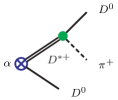
Figure 1: Diagrams contributing to the $D^{0}\,D^{0}\,\pi^{+}$ final state production. Shown here are the $t$-channel diagrams, the $u$-channel ones are obtained by changing $D^{0}(p_{1})\leftrightarrow D^{0}(p_{2})$. Blue, cross vertices: coupling of the source to $D^{\ast}D$ states. Red, square vertices: $D^{\ast}D\to D^{\ast}D$ scattering amplitudes. Green, circle vertices: $D^{\ast}\to D\pi$ amplitudes.

3 Results

3.1 Fit

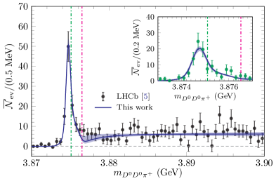
Figure 2: $D^{0}D^{0}\pi^{+}$ spectrum showing the prominent $T_{cc}^{+}$ signal. The data come from the LHCb collaboration [5], and the theoretical curve is calculated with Eq. (3.1), and the parameters of Table 1. The uncertainty is computed through MC bootstrap with resampling of the data, as explained in the text. The inset shows in greater detail the energy region around the peak. The green and purple vertical dashed-dotted lines represent the $D^{\ast+}D^{0}$ and $D^{\ast 0}D^{+}$ thresholds, respectively.

Figure 3: Pull of the theoretical curve with respect to the data for the central fit shown in Fig. 2. The black (green) points corresponds with the $500\ \text{keV}$ ($200\ \text{keV}$) bins.

We aim to compare the event distribution $\mathcal{N}_{\text{ev}}(Q^{2})$ in Eq. (2.11) with the experimental one obtained by the LHCb collaboration [5]. Because of the global normalization, we fix $\alpha=1$ and the free parameters are thus $C_{0}$, $C_{1}$, $\beta$, and $\mathcal{N}_{0}$. To take into account the experimental resolution $\delta\simeq 400\ \text{keV}$, we convolute Eq. (2.11) with an energy resolution function [5, 6],

$$\mathcal{\overline{N}}_{\text{ev}}(Q^{2})=\int\mathrm{d}E\,R_{\text{LHCb }}\left(E,\sqrt{Q^{2}}\right)\,\mathcal{N}_{\text{ev}}(E^{2})~{}.$$ (3.1)

We fit the four free parameters to the available $79$ experimental points ($60$ points in energy bins of $500\ \text{keV}$, and $19$ in energy bins of $200\ \text{keV}$, as can be seen in Fig. 2), obtaining the values in Table 1. The $\chi^{2}$ of the best fit is $\chi^{2}/\text{dof}=71.1/(60+19-4)=0.95$ ($\Lambda=1\ \text{GeV})$ and $70.6/(60+19-4)=0.92$ ($\Lambda=0.5\ \text{GeV}$), and the good agreement with the data can be seen in Fig. 2, where the blue, solid line represents our best fit. The uncertainties are obtained by bootstrapping the fits with Montecarlo (MC) resampling of the data (with $\sim 2000$ MC steps) and thus the correlations are taken into account. As a sanity check, the errors of the parameters are similar to those obtained with Minuit [37] with both minimize and minos. Also, as shown in Fig. 3, the pull of the theoretical curve with respect to the data seems randomly distributed.

Parameter	$\Lambda=1.0\ \text{GeV}$	$\Lambda=0.5\ \text{GeV}$
$C_{0}(\Lambda)\,[\text{fm}^{2}]$	$-0.7008(22)$	$-1.5417(121)$
$C_{1}(\Lambda)\,[\text{fm}^{2}]$	$-0.440(79)$	$-0.71(27)$
$\beta/\alpha$	$0.228(108)$	$0.093(79)$
$\chi^{2}/\text{dof}$	$0.95$	$0.92$

Table 1: Value of the parameters from the fit of the $D^{0}D^{0}\pi^{+}$ event distribution, Eq. (3.1), to the LHCb experimental results [5]. As discussed in Subsec. 3.2, this is the isoscalar solution. The isovector solution, degenerated with the isoscalar one, is obtained by the simultaneous replacement $C_{0}\leftrightarrow C_{1}$ and $\beta\leftrightarrow-\beta$.

Our curve shares some features with the LHCb fit [5], like the prominent $T_{cc}^{+}$ signal (obviously), a sort of small dip around the $D^{\ast 0}D^{+}$ threshold, and a phase-space-like background opening around the $D^{\ast+}D^{0}$ threshold. We note that in this work these features stem from the shape of the $T$-matrix and the production mechanism. Our curve lies a bit higher (and so closer to the data) than the LHCb one at the peak. Near the peak, our curve lies less than $1\sigma$ away from most of the experimental points, also in the zoomed energy region, as can be seen by the pull of the data in Fig. 3.

3.2 Fit degeneracy

We note that under the simultaneous exchange $\beta\to-\beta$ and $C_{0}\leftrightarrow C_{1}$ the $K_{t,u}(Q^{2})$ functions for the $D^{0}D^{0}\pi^{+}$ final state are unchanged. Thus, for any fit that we find with specific values of the free parameters, there is another one with the same $\chi^{2}$ and $\mathcal{\overline{N}}_{\text{ev}}(Q^{2})$, e.g. Fig. 2 remains unchanged. Physically speaking, this reflects the $I_{z}=0$ nature of this specific $D^{\ast}D$ and $DD\pi$ final state, and our inability to distinguish the isospin ($I=0$ or $I=1$) from the $D^{0}D^{0}\pi^{+}$ spectra alone. We will refer to our main fit as isoscalar solution, and the additional one as the isovector one. This symmetry also affects the $I_{z}=0$ $D^{+}D^{+}\pi^{-}$ and $D^{0}D^{+}\pi^{0}$ spectra, and hence each of the three spectra will be equal in both solutions. However, the spectra for the final states with $I_{z}=\pm 1$ ($D^{+}D^{+}\pi^{0}$, $D^{0}D^{+}\pi^{+}$, $D^{+}D^{0}\pi^{-}$, and $D^{0}D^{0}\pi^{0}$, stemming from either $D^{\ast+}D^{+}$ or $D^{\ast 0}D^{0}$), being these purely isovector, do not suffer from this degeneracy in the solution. These spectra, as we will show below, should allow to distinguish the $T_{cc}^{+}$ isospin.

We remark here that, although the $D^{0}D^{0}\pi^{+}$ spectrum alone does not allow to determine the $T_{cc}^{+}$ isospin, the LHCb collaboration has given arguments in favour of its interpretation as an isoscalar state. In particular, in Ref. [6] the experimental spectrum for the $D^{0}D^{+}\pi^{+}$ final state is shown, although with much less statistics than the $D^{0}D^{0}\pi^{+}$ case. Since there is no enhancement near the $D^{\ast+}D^{+}$ threshold, this points to the isoscalar interpretation of $T_{cc}^{+}$. For completeness, though, and in await of more definitive spectra, we show and discuss in what follows both the isoscalar and the isovector solutions, bearing in mind that the isoscalar one is more favoured.

3.3 Pole position, couplings, scattering length

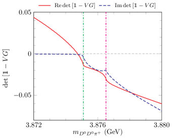
Figure 4: Real (red solid line) and imaginary (blue dashed line) parts of $\det\left[\mathbbm{1}-VG\right]$. The vertical dashed-dotted line represent the $D^{\ast+}D^{0}$ (green) and $D^{\ast 0}D^{+}$ (magenta) thresholds. It can be observed that the real part has a zero very close to the $T_{cc}^{+}$ pole.

The prominent $T_{cc}^{+}$ signal should appear as a bound state pole in the $D^{\ast+}D^{0}$, $D^{\ast 0}D^{+}$ coupled channel $T$-matrix,

$$\sqrt{2m_{D^{\ast}_{i}}m_{D_{i}}}\sqrt{2m_{D^{\ast}_{j}}m_{D_{j}}}T_{ij}(E)=\frac{g_{i}g_{j}}{E^{2}-\left(M_{T_{cc}^{+}}-i\displaystyle\frac{\Gamma_{T_{cc}^{+}}}{2}\right)^{2}}+\cdots~{},$$ (3.2)

and thus as a zero of $\det\left(\mathbbm{1}-V\,G\right)$. In Fig. 4 we show this determinant as a function of the $m_{D^{0}D^{0}\pi^{+}}$ invariant mass. It can be seen that the real part goes through zero close and below the $D^{\ast+}D^{0}$ threshold. However, the imaginary part is not zero because of the finite width of the $D^{\ast}$. For this reason, the pole is indeed not located on the real axis but on the complex plane, and we find:

$$\Delta M_{T_{cc}^{+}}=M_{T_{cc}^{+}}-m_{D^{\ast+}}-m_{D^{0}} =-357(29)\ \text{keV}~{}, \Gamma_{T_{cc}^{+}} =77(1)\ \text{keV} [\Lambda=1.0\ \text{GeV}]~{},$$ (3.3a)

$$=-356(29)\ \text{keV}~{},\, =78(1)\ \text{keV} [\Lambda=0.5\ \text{GeV}]~{}.$$ (3.3b)

Due to the simple parameterization used for the interaction [cf. Eq. (2.4)], the model has freedom to fix the mass of the bound state, but not its width, which in our approach stems essentially from the widths of the $D^{\ast}$ mesons, $\Gamma_{D^{\ast+}}=83.4\ \text{keV}$ and $\Gamma_{D^{\ast 0}}=56.2\ \text{keV}$ (and it is close to the first of them). When compared with the BW determination by the LHCb collaboration in Ref. [5] [cf. Eq. (1.1a)], the value for the masses lie within $1-2\sigma$ deviation, although our width is much smaller than the reported BW one, $\Gamma_{\text{BW}}=410(165)\ \text{keV}$. Indeed, the bound state appears very narrow in the original (i.e. not convoluted) spectrum $\mathcal{N}_{\text{ev}}(m_{D^{0}D^{0}\pi^{+}}^{2})$, as shown in Fig. 5. This not-convoluted spectrum resembles the ones obtained by Ref. [6] (see Extended Data Fig. 8 therein) and Ref. [12]. On the other hand, in the improved analysis of Ref. [6] by the LHCb collaboration [cf. Eq. (1.1b)], an amplitude model is studied that presents a pole at $\Delta M=-360(40)\ \text{keV}$ and $\Gamma=48(2)\ \text{keV}$, being the agreement of our calculation [Eq. (3.3)] much better with this result. Still, our width is larger than that of Ref. [6], so more investigation will be necessary. We point here that our calculation only includes hadronic channels, and thus the width can suffer from systematic deviations.

Figure 5: The $D^{0}D^{0}\pi^{+}$ spectrum before convoluting with the resolution function, as a mass of the $D^{0}D^{0}\pi^{+}$ invariant mass. The very narrow peak corresponds to the $T_{cc}^{+}$ bound state. The vertical dashed-dotted line represent the $D^{\ast+}D^{0}$ (green) and $D^{\ast 0}D^{+}$ (magenta) thresholds.

For the couplings, as defined in Eq. (3.2), we obtain (the imaginary part is negligible):

$$\hphantom{\pm}g_{D^{\ast+}D^{0}} =4.13(12)\ \text{GeV}~{}, \pm g_{D^{\ast 0}D^{+}} =3.53(33)\ \text{GeV}\quad[\Lambda=1.0\ \text{GeV}]~{},$$ (3.4a)

$$=4.36(16)\ \text{GeV}~{}, =3.67(50)\ \text{GeV}\quad[\Lambda=0.5\ \text{GeV}]~{}.$$ (3.4b)

The sign of $g_{D^{\ast 0}D^{+}}$ is negative (positive) in the isoscalar (isovector) solution. In the exact isospin limit, one would have $g_{1}=-g_{2}$ ($g_{1}=+g_{2}$) for an isoscalar (isovector) state (see e.g. Ref. [22]). The fact that both couplings are similar indicates that isospin symmetry is not very broken at the level of interactions, despite the gap between thresholds. The values obtained here are similar to those in Ref. [12], although the difference in the couplings of both channels is larger in our calculation.

We can also compute the scattering length of the $D^{\ast+}D^{0}$ channel, which in our normalization is given by:

$$a_{D^{\ast+}D^{0}}=-\frac{\mu_{1}}{2\pi}T_{11}(E^{1}_{\text{th}})~{},$$ (3.5)

and we get:

$$a_{D^{\ast+}D^{0}} =-7.99(46)+i\,2.21(28)\ \text{fm}\quad[\Lambda=1.0\ \text{GeV}]~{},$$ (3.6a)

$$=-8.56(49)+i\,2.61(32)\ \text{fm}\quad[\Lambda=0.5\ \text{GeV}]~{}.$$ (3.6b)

The imaginary part does not vanish because the $D^{\ast+}D^{0}$ system decays to $DD\pi$ (which in our approach is taken into account by the presence of the $D^{\ast}$ widths), and it is sizeable because the width of the $T_{cc}^{+}$, though small, is not negligible when compared to its binding energy. These values are similar to those obtained in Ref. [6].

3.4 Molecular state?

The Weinberg compositeness criterium [38] is often used to assess the “molecularness” of a given state, and there is quite a lot of activity in this topic (see e.g. Refs. [39, 40, 41, 42, 43, 44, 45, 46, 47] and references therein). A generalization to coupled channels performed in Ref. [40] allows to interpret the quantities $P_{i}$,

$$P_{i}=-g_{i}^{2}\frac{\mathrm{d}G(E^{2})}{\mathrm{d}E^{2}}~{},$$ (3.7)

as the probabilities of finding the bound state in a given channel. We find the values:

$$\hphantom{\pm}P_{D^{\ast+}D^{0}} =0.77(4)~{}, P_{D^{\ast 0}D^{+}} =0.23(4)~{}, [\Lambda=1.0\ \text{GeV}]~{},$$ (3.8a)

$$=0.79(5)~{}, =0.21(5)~{}, [\Lambda=0.5\ \text{GeV}]~{},$$ (3.8b)

which turn out to be remarkably independent of the cutoff $\Lambda$. In the exact isospin limit, one can check that the probabilities are $P_{D^{\ast+}D^{0}}=P_{D^{\ast 0}D^{+}}=0.5$, or, in terms of definite isospin states, the molecular probability is exactly one, $P_{I}=1$ (regardless of the isospin $I=0$ or $I=1$ of the state, see Subsec. 3.2). However, it must be said that the fact that $P_{I}=1$ (or equivalently $P_{D^{\ast+}D^{0}}+P_{D^{\ast 0}D^{+}}=1$) is strictly built in the model and in Eq. (3.7) due to the simple, constant parameterization of the $V$ matrix [cf. Eq. (2.4)]. It is not a consequence of the specific values of the constants $C_{I}(\Lambda)$.

We next discuss the results that are obtained when the original Weinberg arguments [38] (see also Ref. [47]) about the compositeness are used. Certainly, the $T_{cc}^{+}$ bound state that we obtain seems to satisfy the three applicability requirements (stable or very narrow state, coupling to a two-channel threshold not much above the location of the state, and $S$-wave) of Ref. [38]. The formula for the molecular probability reads:

$$P_{I}=\sqrt{\frac{1}{1+\left\lvert\displaystyle\frac{2r_{I}}{a_{I}}\right\rvert}}~{}.$$ (3.9)

For simplicity, we discuss the results in the isospin and zero $D^{\ast}$ width limits, where the concept of molecule should make more sense. In the isospin limit, the $D^{\ast+}D^{0}$ and $D^{\ast 0}D^{+}$ $T$-matrix can be diagonalized into $I=0$ and $I=1$ amplitudes, $T_{I}(E)=C_{I}^{-1}-G(E)$. The $T_{cc}^{+}$ is in this case a bound state with zero width too, and the scattering length and effective range, that we denote now $a_{I}$ and $r^{0}_{I}$, are also real. We find:

$$a_{I} =-5.18(16)\ \text{fm}~{}, r_{I} =0.63\ \text{fm}~{}, P_{I} =0.897(3)~{}, [\Lambda=1.0\ \text{GeV}]~{},$$ (3.10a)

$$=-5.57(25)\ \text{fm}~{}, =1.26\ \text{fm}~{}, =0.830(5)~{}, [\Lambda=0.5\ \text{GeV}]~{}.$$ (3.10b)

We see that a large molecular component between $80\%$–$90\%$ is obtained. Because of the constant value taken for the kernels $V_{I}=C_{I}(\Lambda)$, the effective range $r$ is solely determined by the cutoff, and does not depend on the $C_{I}(\Lambda)$ values, which can affect the determination of the molecular probability. That being said, in Appendix B we have investigated more complex parameterizations of the matrix elements of $V$, that would allow better determinations of the effective range $r$. While these alternative parameterizations improve slightly the quality of the fit, they do not change dramatically this probability. The molecular probability is always large, and thus our conclusion is that the molecular description fits nicely for the $T_{cc}^{+}$.

4 Predictions

4.1 Predictions of the spectrum for different $DD\pi$ final states

As previously mentioned, the $D^{0}D^{0}\pi^{+}$ spectrum alone does not allow to determine the $T_{cc}^{+}$ isospin. Instead, other $DD\pi$ spectra are needed, and hence we make a prediction of such additional spectra here, independently of the nature of the $T_{cc}^{+}$ state.

$D^{+}\pi^{-}D^{+}\to$ $+$ $+$

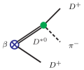
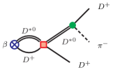
Figure 6: Same as Fig. 1, but for the $D^{+}\,D^{+}\,\pi^{-}$ final state production.

$D^{0}\pi^{0}D^{+}\to$ $+$ $+$
$D^{0}\pi^{0}D^{+}$$+$ $+$ $+$

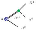
Figure 7: Diagrams contributing to the $D^{+}D^{0}\pi^{0}$ production. $t$- and $u$-channels are explicitly shown.

The amplitudes for the final states $D^{+}D^{+}\pi^{-}$ and $D^{0}D^{+}\pi^{0}$, with $I_{z}=0$ too, are diagramatically shown in Figs. 6 and 7, respectively. Assuming the same production mechanisms and the same resolution as in the $D^{0}D^{0}\pi^{+}$ case, and ignoring possible differences in the reconstruction efficiencies of particles in the final states, we can predict the spectra for these final states. These are shown in Fig. 8, and for the sake of comparison we have assumed the same normalization (i.e. statistics).

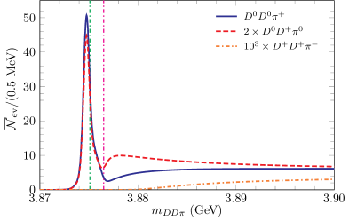
Figure 8: Predictions of the spectra for other $DD\pi$ final states with $I_{z}=0$. The same production mechanism and resolution as in the $D^{0}D^{0}\pi^{+}$ case (shown in Fig. 2 and also here) are assumed. To facilitate the comparison, some of the spectra have been scaled. The vertical dashed-dotted line represent the $D^{\ast+}D^{0}$ (green) and $D^{\ast 0}D^{+}$ (magenta) thresholds.

The $D^{+}D^{+}\pi^{-}$ threshold lies $\sim 10\ \text{MeV}$ above the $D^{0}D^{0}\pi^{+}$ (and $D^{+}D^{0}\pi^{0}$) threshold, which makes a huge difference given the $30\ \text{MeV}$ spanned by the data and the narrowness of the $T_{cc}^{+}$ signal. In addition, the decaying $D^{\ast}$ in this channel is always a $D^{\ast 0}$, which has a smaller width than that of $D^{\ast+}$. All in all, these phase-space facts make it so that the number of events in the $D^{+}D^{+}\pi^{-}$ spectrum is negligible, and there is no trace of the $T_{cc}^{+}$, as can be seen in Fig. 8 (dashed-dotted orange line). On the other hand, this does not happen for the $D^{+}D^{0}\pi^{0}$ final state, and as shown in Fig. 8 (dashed red line) the spectrum is comparable to (but smaller than) that of the $D^{0}D^{0}\pi^{+}$ final state (solid blue line). Therefore, this channel could be used to confirm the existence of the $T_{cc}^{+}$ state. As explained in Subsec. 3.2, the predicted spectra for these final states, shown in Fig. 8, are the same for both the isoscalar and the isovector solutions.

$+$	$+$
$+$	$+$

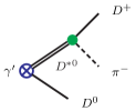
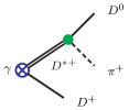
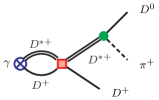
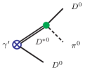
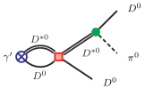
Figure 9: Diagrams contributing to final states with $I_{z}=\pm 1$.

We can also predict the spectrum for the $I_{z}=\pm 1$ final states, where the difference between both solutions should be visible. The diagrams used to compute these spectra are shown in Fig. 9, and the line shapes (taking into account also here the resolution) are shown in Fig. 10. Similarly as for $D^{+}D^{+}\pi^{-}$ case, the $D^{0}D^{+}\pi^{-}$ distribution is negligible due to the lack of phase space, and thus not shown in Fig. 9.

Figure 10: Prediction of the spectra for $DD\pi$ final states with $I_{z}=\pm 1$. The green and magenta vertical dashed-dotted lines represent the $D^{\ast 0}D^{0}$ and $D^{\ast+}D^{+}$ thresholds, respectively. The thick solid (thin dashed) lines represent the spectra obtained when the isoscalar (isovector) solution is used. Different colors (blue, brown, and red) represent different final state ($D^{+}D^{+}\pi^{0}$, $D^{0}D^{+}\pi^{+}$, and $D^{0}D^{0}\pi^{0}$, respectively) spectra. The green and magenta vertical dashed-dotted lines mark the $D^{\ast 0}D^{0}$ and $D^{\ast+}D^{+}$ thresholds, respectively. As explained in the text, the distribution for the $D^{0}D^{+}\pi^{-}$ final state is negligible and not shown here.

The spectra predicted for the isoscalar solution (solid thick lines in Fig. 10) show no enhancement at threshold nor additional states, and are smooth phase-space distributions. In the isovector solution, since the $T_{cc}^{+}$ would have $I=1$, one thus expects the other two members of the isospin triplet, $T_{cc}^{++}$ and $T_{cc}^{0}$ to show up in these spectra, as seen indeed (dashed thin lines) in Fig. 10. In this solution we find two additional poles with the following binding energies:

$$\Delta M_{T_{cc}^{++}}=M_{T_{cc}^{++}}-m_{D^{\ast+}}-m_{D^{+}} =-873(53)\ \text{keV}\quad[\Lambda=1.0\ \text{GeV}]~{},$$ (4.1a)

$$=-842(67)\ \text{keV}\quad[\Lambda=0.5\ \text{GeV}]~{},$$ (4.1b)

$$\Delta M_{T_{cc}^{0}}=M_{T_{cc}^{0}}-m_{D^{\ast 0}}-m_{D^{0}} =-838(52)\ \text{keV}\quad[\Lambda=1.0\ \text{GeV}]~{},$$ (4.2a)

$$=-825(67)\ \text{keV}\quad[\Lambda=0.5\ \text{GeV}]~{}.$$ (4.2b)

These states would be somewhat more bound than the $T_{cc}^{+}$ because there is a single channel/threshold. Finally, we must stress that the $D^{+}D^{0}\pi^{+}$ spectrum shown in Ref. [6] by the LHCb collaboration, albeit with wide bins, agrees with the shape of the $D^{+}D^{0}\pi^{+}$ spectrum predicted in the isoscalar solution (thick solid green line in Fig. 10), and not with the isovector one (thin dashed green line). As discussed in Subsec. 3.2, this fact favours the $I=0$ interpretation of $T_{cc}^{+}$ and thus our isoscalar solution.

4.2 Heavy Quark Spin Symmetry partners of $T_{cc}^{+}$

Heavy-Quark Spin Symmetry (HQSS) [48, 49] predicts that heavy-meson interactions are independent of the heavy-quark spin. Similar to the $D^{(\ast)}\bar{D}^{(\ast)}$ case [50, 51], HQSS predicts that, up to $\mathcal{O}(1/M_{Q})$, the interaction kernels of the $I(J^{P})$ $D^{\ast}D^{\ast}$ systems are related to those of the $D^{\ast}D$ ones as:

$$\left\langle D^{\ast}D^{\ast},\,0(1^{+})\right\rvert\hat{V}\left\lvert D^{\ast}D^{\ast},\,0(1^{+})\right\rangle =\left\langle D^{\ast}D,\,0(1^{+})\right\rvert\hat{V}\left\lvert D^{\ast}D,\,0(1^{+})\right\rangle=V_{0}~{},$$ (4.3a)

$$\left\langle D^{\ast}D^{\ast},\,1(2^{+})\right\rvert\hat{V}\left\lvert D^{\ast}D^{\ast},\,1(2^{+})\right\rangle =\left\langle D^{\ast}D,\,1(1^{+})\right\rvert\hat{V}\left\lvert D^{\ast}D,\,1(1^{+})\right\rangle=V_{1}~{}.$$ (4.3b)

For instance, Ref. [52] predicts the existence of twin (isoscalar) bound states very close (a few MeV) to the $D^{\ast}D^{(\ast)}$ threshold. Based on Eq. (4.3), for each of the $D^{\ast}D$ solutions (isoscalar or isovector) we can predict an additional $D^{\ast}D^{\ast}$ state, that we denote $T_{cc}^{\ast}$. If the isoscalar solution holds, we predict an $I(J^{P})=0(1^{+})$ HQSS partner of the $T_{cc}^{+}$ below the $D^{\ast+}D^{\ast 0}$ threshold, with mass:

$$\Delta M_{{T_{cc}^{\ast+}}}=M_{{T_{cc}^{\ast+}}}-m_{D^{\ast+}}-m_{D^{\ast 0}} =-1561(71)\ \text{keV}~{},\quad[\Lambda=1.0\ \text{GeV}]~{},$$ (4.4a)

$$=-1148(79)\ \text{keV}~{},\quad[\Lambda=0.5\ \text{GeV}]~{}.$$ (4.4b)

If instead the isovector solution is taken, we predict a $1(2^{+})$ (isospin triplet), with masses:

$$\Delta M_{T_{cc}^{\ast++}}=M_{T_{cc}^{\ast++}}-2m_{D^{\ast+}} =-1580(71)\ \text{keV}~{},\quad[\Lambda=1.0\ \text{GeV}]~{},$$ (4.5a)

$$=-1156(79)\ \text{keV}~{},\quad[\Lambda=0.5\ \text{GeV}]~{},$$ (4.5b)

$$\Delta M_{{T_{cc}^{\ast+}}}=M_{{T_{cc}^{\ast+}}}-m_{D^{\ast+}}-m_{D^{\ast 0}} =-1561(71)\ \text{keV}~{},\quad[\Lambda=1.0\ \text{GeV}]~{},$$ (4.5c)

$$=-1148(79)\ \text{keV}~{},\quad[\Lambda=0.5\ \text{GeV}]~{}.$$ (4.5d)

$$\Delta M_{T_{cc}^{\ast 0}}=M_{T_{cc}^{\ast 0}}-2m_{D^{\ast 0}} =-1543(71)\ \text{keV}~{},\quad[\Lambda=1.0\ \text{GeV}]~{},$$ (4.5e)

$$=-1140(79)\ \text{keV}~{},\quad[\Lambda=0.5\ \text{GeV}]~{}.$$ (4.5f)

Since the decays of the $T_{cc}^{\ast}$ can be quite involved, we do not predict its width, which should be further investigated. As already explained (Subsec. 3.2 and  4.1), the isoscalar solution is favoured, and hence the prediction Eq. (4.4) of an isoscalar state as a HQSS partner of the $T_{cc}^{+}$ seems the most plausible one.

5 Conclusions

In this work we have performed a coupled channel analysis of the $D^{\ast}D$ system, in view of the recent results by the LHCb collaboration [5, 6] claiming the existence of a new state, $T_{cc}^{+}$, seen as a clear signal in the $D^{0}D^{0}\pi^{+}$ spectrum. In our analysis we reproduce the experimental spectrum, and we obtain that the $T_{cc}^{+}$ appears as a bound state in the $D^{\ast}D$ amplitude. The bound state shows a large molecular component. While the analysis of Ref. [6] shows no enhancement near the $D^{\ast+}D^{0}$ threshold in the $D^{0}D^{+}\pi^{+}$ spectrum, thus favouring the $I=0$ interpretation of $T_{cc}^{+}$ (our isoscalar solution), more data will be welcome to definitely settle the question. Independently of the nature of the $T_{cc}^{+}$ state, we have predicted the shape of other $DD\pi$ spectra in which the $T_{cc}^{+}$ can be seen, and in which the isospin of this state could be determined. Finally, based on Heavy-Quark Spin Symmetry, we have predicted the existence of an isospin singlet or triplet (most likely a singlet, because the isoscalar solution seems to be favoured) of $D^{\ast}D^{\ast}$ states, $1$–$2\ \text{MeV}$ below the $D^{\ast}D^{\ast}$ thresholds.

Appendix A $K_{t,u}(Q^{2})$ functions

For completeness, we show here the specific $K_{t,u}(Q^{2})$ of the possible $DD\pi$ final states (with $I=0$ or $1$) discussed in this work, and shown schematically in Figs. 1, 6, 7, and 9:

• $\pi^{+}D^{0}D^{0}$

  $$K_{t}(Q^{2}) =\alpha\left(1+G_{1}(Q^{2})T_{11}(Q^{2})\right)C_{D^{\ast+}\to D^{0}\pi^{+}}+\beta G_{2}(Q^{2})T_{12}(Q^{2})\,C_{D^{\ast+}\to D^{0}\pi^{+}}~{},$$ (A.1a)

  $$K_{u}(Q^{2}) =K_{t}(Q^{2})~{}.$$ (A.1b)

• $\pi^{-}D^{+}D^{+}$

  $$K_{t}(Q^{2}) =\beta\left(1+G_{2}(Q^{2})T_{22}(Q^{2})\right)C_{D^{\ast 0}\to D^{+}\pi^{-}}+\alpha G_{1}(Q^{2})T_{12}(Q^{2})\,C_{D^{\ast 0}\to D^{+}\pi^{-}}~{},$$ (A.2a)

  $$K_{u}(Q^{2}) =K_{t}(Q^{2})~{}.$$ (A.2b)

• $\pi^{0}D^{0}D^{+}$

  $$K_{t}(Q^{2}) =\beta\left(1+G_{2}(Q^{2})T_{22}(Q^{2})\right)C_{D^{\ast 0}\to D^{0}\pi^{0}}+\alpha G_{1}(Q^{2})T_{12}(Q^{2})\,C_{D^{\ast 0}\to D^{0}\pi^{0}}~{},$$ (A.3a)

  $$K_{u}(Q^{2}) =\alpha\left(1+G_{1}(Q^{2})T_{11}(Q^{2})\right)C_{D^{\ast+}\to D^{+}\pi^{0}}+\beta G_{2}(Q^{2})T_{12}(Q^{2})\,C_{D^{\ast+}\to D^{+}\pi^{0}}~{}.$$ (A.3b)

• $\pi^{0}D^{+}D^{+}$

  $$K_{t}(Q^{2}) =\gamma\left(1+G_{D^{\ast+}D^{+}}(Q^{2})T_{D^{\ast+}D^{+}}(Q^{2})\right)C_{D^{\ast+}\to D^{+}\pi^{0}}~{},$$ (A.4a)

  $$K_{u}(Q^{2}) =K_{t}(Q^{2})~{}.$$ (A.4b)

• $\pi^{+}D^{0}D^{+}$

  $$K_{t}(Q^{2}) =\gamma\left(1+G_{D^{\ast+}D^{+}}(Q^{2})T_{D^{\ast+}D^{+}}(Q^{2})\right)C_{D^{\ast+}\to D^{0}\pi^{+}}~{},$$ (A.5a)

  $$K_{u}(Q^{2}) =0~{}.$$ (A.5b)

• $\pi^{-}D^{+}D^{0}$

  $$K_{t}(Q^{2}) =\gamma^{\prime}\left(1+G_{D^{\ast 0}D^{0}}(Q^{2})T_{D^{\ast 0}D^{0}}(Q^{2})\right)C_{D^{\ast 0}\to D^{+}\pi^{-}}~{},$$ (A.6a)

  $$K_{u}(Q^{2}) =0~{}.$$ (A.6b)

• $\pi^{0}D^{0}D^{0}$

  $$K_{t}(Q^{2}) =\gamma^{\prime}\left(1+G_{D^{\ast 0}D^{0}}(Q^{2})T_{D^{\ast 0}D^{0}}(Q^{2})\right)C_{D^{\ast 0}\to D^{0}\pi^{0}}~{}.$$ (A.7a)

  $$K_{u}(Q^{2}) =K_{t}(Q^{2})~{}.$$ (A.7b)

Appendix B Different parameterizations of the interaction kernels

Figure 11: $D^{0}D^{0}\pi^{+}$ spectra obtained for the alternative fits discussed in Appendix B, Eqs. (B.1). The pink band represents the uncertainty of the main fit discussed in Subsec. 3.1, and is shown here for reference.

In this Appendix we explore the possibility of using different parameterizations for the kernels $V_{I=0,1}$. For concreteness, we take the case $\Lambda=0.5\ \text{GeV}$ to compare with our main results in Sec. 3. The variations that we take for our interaction kernels $V_{I}(s)$ are as follows:

$$V_{0}(s)=C_{0}(\Lambda) \quad\longrightarrow\quad V_{0}(s)=C_{0}(\Lambda)+b_{0}(\Lambda)k^{2}~{},$$ (B.1a)

$$V_{0}(s)=C_{0}(\Lambda) \quad\longrightarrow\quad V_{0}(s)=\frac{d_{0}(\Lambda)}{E-M_{0}(\Lambda)}~{},$$ (B.1b)

$$V_{1}(s)=C_{1}(\Lambda) \quad\longrightarrow\quad V_{1}(s)=C_{1}(\Lambda)+b_{1}(\Lambda)k^{2}~{}.$$ (B.1c)

The parameters obtained in the fits are:

• Eq. (B.1a):

  $$C_{0}(\Lambda)=-1.52\ \text{fm}^{2}~{},\ b_{0}(\Lambda)=0.6\ \text{fm}^{4}~{},\ C_{1}(\Lambda)=-0.54\ \text{fm}^{2}~{},\$$

  $$\beta/\alpha=0.098~{},\ \chi^{2}/\text{dof}=0.94$$ (B.2a)

• Eq. (B.1b):

  $$d_{0}(\Lambda)=-41\ \text{MeV}\cdot\text{fm}^{2}~{},\ M_{0}=3848\ \text{MeV}~{},\ C_{1}(\Lambda)=-0.50\ \text{fm}^{2}~{},\$$

  $$\beta/\alpha=0.160~{},\ \chi^{2}/\text{dof}=0.90$$ (B.2b)

• Eq. (B.1c):

  $$C_{0}(\Lambda)=-1.55\ \text{fm}^{2}~{},\ C_{1}(\Lambda)=-0.54\ \text{fm}^{2}~{},\ b_{1}(\Lambda)=-0.7\ \text{fm}^{4}~{},\$$

  $$\beta/\alpha=0.030~{},\ \chi^{2}/\text{dof}=0.94$$ (B.2c)

The resulting spectrum for each of these fits is shown in Fig. 11, and as can be seen they all lie essentially within the uncertainty band of the main fit discussed in Subsec. 3.1, which justifies taking our fit in Subsec. 3.1 as our main one. Some of the output quantities ($T_{cc}^{+}$ mass and width, etc.) are shown in Table 2 for the different fits. The fitted parameters in Eqs. (B.2) can show deviations across the fits with respect to the main fit in Table 1 which are larger than the statistical uncertainty. E.g., $C_{0}(\Lambda)=-1.5417(121)\ \text{fm}^{2}$ in the main fit, but here one can have deviations of about $0.03\ \text{fm}^{2}$, larger than the statistical one, which is $\sim 0.01\ \text{fm}^{2}$. This seems to be the case too for the width and the couplings of the $T_{cc}^{+}$, but not for the mass. If we now pay attention to the molecular probability, calculated in the isospin limit as Eq. (3.9) (last row in Table 2), we see that in all cases we still have $P_{I}\geqslant 0.75$, i.e. even when more complex parameterizations are allowed one still finds a very large molecular component.

	(B.1a)	(B.1b)	(B.1c)	Main
$\Delta M_{T_{cc}^{+}}\ \text{(keV)}$	$-350$	$-357$	$-355$	$-356(29)$
$\Gamma\ \text{(keV)}$	$78$	$106$	$77$	$78(1)$
$g_{D^{\ast+}D^{0}}\ \text{(GeV)}$	$4.61$	$5.03$	$4.27$	$4.36(16)$
$g_{D^{\ast 0}D^{+}}\ \text{(GeV)}$	$4.24$	$4.68$	$3.97$	$3.67(50)$
$a_{D^{\ast+}D^{0}}\ \text{(fm)}$	$-9.26+2.98i$	$-9.87+3.59i$	$-8.36+2.48i$	$-8.56(49)+2.61(32)i$
$P_{D^{\ast+}D^{0}}$	$0.89$	$1.05$	$0.76$	$0.79(5)$
$P_{D^{\ast 0}D^{+}}$	$0.28$	$0.34$	$0.24$	$0.21(5)$
$a_{I}\ \text{(fm)}$	$-6.27$	$-6.65$	$-5.29$	$-5.57(25)$
$r_{I}\ \text{(fm)}$	$1.95$	$2.51$	$1.26$	$1.26$
$P_{I}$ [Eq. (3.9)]	$0.79$	$0.76$	$0.82$	$0.830(5)$

Table 2: Values of different output quantities discussed in Sec. 3 when the different parameterizations Eqs. (B.1) are employed. In the last column, for reference, we show the result obtained in the main fit.

References

- [1] M. Gell-Mann, A Schematic Model of Baryons and Mesons, Phys. Lett. 8 (1964) 214.
- [2] G. Zweig, An SU(3) model for strong interaction symmetry and its breaking. Version 1, CERN-TH-401.
- [3] G. Zweig, An SU(3) model for strong interaction symmetry and its breaking. Version 2, in DEVELOPMENTS IN THE QUARK THEORY OF HADRONS. VOL. 1. 1964 - 1978, D.B. Lichtenberg and S.P. Rosen, eds., pp. 22–101 (1964).
- [4] S. Godfrey and N. Isgur, Mesons in a Relativized Quark Model with Chromodynamics, Phys. Rev. D 32 (1985) 189.
- [5] R. Aaij et al., LHCb collaboration, Observation of an exotic narrow doubly charmed tetraquark, 2109.01038.
- [6] R. Aaij et al., LHCb collaboration, Study of the doubly charmed tetraquark , 2109.01056.
- [7] R. Aaij et al., LHCb collaboration, Observation of the doubly charmed baryon , Phys. Rev. Lett. 119 (2017) 112001 [1707.01621].
- [8] X.-K. Dong, F.-K. Guo and B.-S. Zou, A survey of heavy-heavy hadronic molecules, 2108.02673.
- [9] N. Li, Z.-F. Sun, X. Liu and S.-L. Zhu, Perfect molecular prediction matching the observation at LHCb, Chin. Phys. Lett. 38 (2021) 092001 [2107.13748].
- [10] L. Meng, G.-J. Wang, B. Wang and S.-L. Zhu, Probing the long-range structure of the Tcc+ with the strong and electromagnetic decays, Phys. Rev. D 104 (2021) 051502 [2107.14784].
- [11] L.-Y. Dai, X. Sun, X.-W. Kang, A.P. Szczepaniak and J.-S. Yu, Pole analysis on the doubly charmed meson in mass spectrum, 2108.06002.
- [12] A. Feijoo, W.H. Liang and E. Oset, mass distribution in the production of the exotic state, 2108.02730.
- [13] S.S. Agaev, K. Azizi and H. Sundu, Newly observed exotic doubly charmed meson , 2108.00188.
- [14] T.-W. Wu, Y.-W. Pan, M.-Z. Liu, S.-Q. Luo, X. Liu and L.-S. Geng, Discovery of the doubly charmed state implies a triply charmed hexaquark state, 2108.00923.
- [15] X.-Z. Ling, M.-Z. Liu, L.-S. Geng, E. Wang and J.-J. Xie, Can we understand the decay width of the state?, 2108.00947.
- [16] R. Chen, Q. Huang, X. Liu and S.-L. Zhu, Another doubly charmed molecular resonance , 2108.01911.
- [17] M.-J. Yan and M.P. Valderrama, Subleading contributions to the decay width of the tetraquark, 2108.04785.
- [18] X.-Z. Weng, W.-Z. Deng and S.-L. Zhu, Doubly heavy tetraquarks in an extended chromomagnetic model, 2108.07242.
- [19] Y. Huang, H.Q. Zhu, L.-S. Geng and R. Wang, Production of the state in the reaction, 2108.13028.
- [20] R. Chen, N. Li, Z.-F. Sun, X. Liu and S.-L. Zhu, Doubly charmed molecular pentaquarks, Phys. Lett. B 822 (2021) 136693 [2108.12730].
- [21] Q. Xin and Z.-G. Wang, Analysis of the axialvector doubly-charmed tetraquark molecular states with the QCD sum rules, 2108.12597.
- [22] S. Fleming, R. Hodges and T. Mehen, decays: differential spectra and two-body final states, 2109.02188.
- [23] X. Chen, Doubly heavy tetraquark states and , 2109.02828.
- [24] K. Azizi and U. Özdem, Magnetic dipole moments of the and tetraquark states, 2109.02390.
- [25] H. Ren, F. Wu and R. Zhu, Hadronic molecule interpretation of and its beauty-partners, 2109.02531.
- [26] G. Yang, J. Ping and J. Segovia, Hidden-charm tetraquarks with strangeness in the chiral quark model, 2109.04311.
- [27] Y. Jin, S.-Y. Li, Y.-R. Liu, Q. Qin, Z.-G. Si and F.-S. Yu, Colour and baryon number fluctuation of preconfinement system in production process and structure, 2109.05678.
- [28] Y. Hu, J. Liao, E. Wang, Q. Wang, H. Xing and H. Zhang, The production of doubly charmed exotic hadrons in heavy ion collisions, 2109.07733.
- [29] K. Chen, R. Chen, L. Meng, B. Wang and S.-L. Zhu, Systematics of the heavy flavor hadronic molecules, 2109.13057.
- [30] J. He, D.-Y. Chen, Z.-W. Liu and X. Liu, New clean fission with hadronic molecular states, 2109.14395.
- [31] P. Junnarkar, N. Mathur and M. Padmanath, Study of doubly heavy tetraquarks in Lattice QCD, Phys. Rev. D 99 (2019) 034507 [1810.12285].
- [32] Y. Ikeda, B. Charron, S. Aoki, T. Doi, T. Hatsuda, T. Inoue et al., Charmed tetraquarks and from dynamical lattice QCD simulations, Phys. Lett. B 729 (2014) 85 [1311.6214].
- [33] G.K.C. Cheung, C.E. Thomas, J.J. Dudek and R.G. Edwards, Hadron Spectrum collaboration, Tetraquark operators in lattice QCD and exotic flavour states in the charm sector, JHEP 11 (2017) 033 [1709.01417].
- [34] A. Francis, R.J. Hudspith, R. Lewis and K. Maltman, Evidence for charm-bottom tetraquarks and the mass dependence of heavy-light tetraquark states from lattice QCD, Phys. Rev. D 99 (2019) 054505 [1810.10550].
- [35] L. Leskovec, S. Meinel, M. Pflaumer and M. Wagner, Lattice QCD investigation of a doubly-bottom tetraquark with quantum numbers , Phys. Rev. D 100 (2019) 014503 [1904.04197].
- [36] P.A. Zyla et al., Particle Data Group collaboration, Review of Particle Physics, PTEP 2020 (2020) 083C01.
- [37] F. James, MINUIT Function Minimization and Error Analysis: Reference Manual Version 94.1, .
- [38] S. Weinberg, Evidence That the Deuteron Is Not an Elementary Particle, Phys. Rev. 137 (1965) B672.
- [39] V. Baru, J. Haidenbauer, C. Hanhart, Y. Kalashnikova and A.E. Kudryavtsev, Evidence that the a(0)(980) and f(0)(980) are not elementary particles, Phys. Lett. B 586 (2004) 53 [hep-ph/0308129].
- [40] D. Gamermann, J. Nieves, E. Oset and E. Ruiz Arriola, Couplings in coupled channels versus wave functions: application to the X(3872) resonance, Phys. Rev. D 81 (2010) 014029 [0911.4407].
- [41] J. Yamagata-Sekihara, J. Nieves and E. Oset, Couplings in coupled channels versus wave functions in the case of resonances: application to the two states, Phys. Rev. D 83 (2011) 014003 [1007.3923].
- [42] T. Hyodo, D. Jido and A. Hosaka, Compositeness of dynamically generated states in a chiral unitary approach, Phys. Rev. C 85 (2012) 015201 [1108.5524].
- [43] F. Aceti and E. Oset, Wave functions of composite hadron states and relationship to couplings of scattering amplitudes for general partial waves, Phys. Rev. D 86 (2012) 014012 [1202.4607].
- [44] Z.-H. Guo and J.A. Oller, Probabilistic interpretation of compositeness relation for resonances, Phys. Rev. D 93 (2016) 096001 [1508.06400].
- [45] T. Sekihara, T. Hyodo and D. Jido, Comprehensive analysis of the wave function of a hadronic resonance and its compositeness, PTEP 2015 (2015) 063D04 [1411.2308].
- [46] J.A. Oller, New results from a number operator interpretation of the compositeness of bound and resonant states, Annals Phys. 396 (2018) 429 [1710.00991].
- [47] I. Matuschek, V. Baru, F.-K. Guo and C. Hanhart, On the nature of near-threshold bound and virtual states, Eur. Phys. J. A 57 (2021) 101 [2007.05329].
- [48] M. Neubert, Heavy quark symmetry, Phys. Rept. 245 (1994) 259 [hep-ph/9306320].
- [49] A.V. Manohar and M.B. Wise, Heavy quark physics, vol. 10 (2000).
- [50] C. Hidalgo-Duque, J. Nieves and M.P. Valderrama, Light flavor and heavy quark spin symmetry in heavy meson molecules, Phys. Rev. D 87 (2013) 076006 [1210.5431].
- [51] F.-K. Guo, C. Hidalgo-Duque, J. Nieves and M.P. Valderrama, Consequences of Heavy Quark Symmetries for Hadronic Molecules, Phys. Rev. D 88 (2013) 054007 [1303.6608].
- [52] M.-Z. Liu, T.-W. Wu, M. Pavon Valderrama, J.-J. Xie and L.-S. Geng, Heavy-quark spin and flavor symmetry partners of the X(3872) revisited: What can we learn from the one boson exchange model?, Phys. Rev. D 99 (2019) 094018 [1902.03044].