Geometrothermodynamics of van der Waals systems
Abstract
We explore the properties of the equilibrium space of van der Waals thermodynamic systems. We use an invariant representation of the fundamental equation by using the law of corresponding states, which allows us to perform a general analysis for all possible van der Waals systems. The investigation of the equilibrium space is performed by using the Legendre invariant formalism of geometrothermodynamics, which guarantees the independence of the results from the choice of thermodynamic potential. We find all the curvature singularities of the equilibrium space that correspond to first and second order phase transitions. We compare our results with those obtained by using Hessian metrics for the equilibrium space. We conclude that the formalism of geometrothermodynamics allows us to determine the complete phase transition structure of systems with two thermodynamic degrees of freedom.
pacs:
05.70.-a; 02.40.-kI Introduction
Differential geometry is an important mathematical discipline that has found very broad applications in physics, chemistry, and engineering Frankel (2004). For instance, in Nature there exist so far only four fundamental interactions and all of them can be described by using concepts of differential geometry such as manifolds, metrics, connections, fiber bundles, etc.
In thermodynamics, differential geometry has been also applied intensively, providing an alternative way to describe thermodynamic systems. The starting point is the equilibrium space that is an abstract space whose points can be interpreted as representing equilibrium states of the system. One of the first attempts to introduce differential geometry in thermodynamics was proposed by Rao Rao (1945) by introducing a Riemannian metric related to Fisher’s information matrix. Rao’s proposal has found many applications in statistical physics, information theory, and thermodynamics Amari (2012). Furthermore, Hessian metrics can also be postulated to describe the geometric properties of the equilibrium space. In particular, Weinhold Weinhold (1975) and Ruppeiner Ruppeiner (1979, 1995) proposed to use the Hessian of the thermodynamic potentials known as internal energy and entropy, respectively, as metrics for the equilibrium space. The theoretical framework in which Hessian metrics are applied to describe the equilibrium space is usually referred to as thermodynamic geometry.
More recently, one of us Quevedo (2007) proposed the alternative approach of geometrothermodynamics (GTD), in which the metrics of the equilibrium space should be independent of the choice of thermodynamic potential. This is a characteristic of classical equilibrium thermodynamics Callen (1985), which implies that the properties of a system are invariant with respect to changes of the thermodynamic potential, i.e., invariant with respect to Legendre transformations. Another important characteristic of equilibrium thermodynamics is that all the properties of the systems are completely determined by the corresponding fundamental equations Callen (1985). In GTD, the existence of a fundamental equation and Legendre invariance are the main assumptions that are used to construct the equilibrium space.
Thermodynamic geometry and GTD have been used to investigate ordinary laboratory systems as well as more exotic systems like black holes; see, for instance, Weinhold (2009); Ruppeiner (2014); Åman et al. (2015); Mandal and Biswas (2015); Bravetti and Luongo (2014); Hendi et al. (2016); Kubizňák and Mann (2015). In this work, we apply the formalism of GTD to investigate the physical properties of van der Waals systems. In particular, we clarify the relationship between the three different Legendre invariant metrics that are known in GTD. In fact, we find the curvature singularities of the corresponding equilibrium space and show that they correspond to the complete phase transition structure of van der Waals systems. We compare our results with those obtained by using Hessian metrics and show that whereas the GTD metrics contain information about the first and second order phase transitions, Hessian metrics are related to first order phase transitions only.
This work is organized as follows. In Sec. II, we present the basic ingredients of GTD. Section III is dedicated to the derivation of the reduced fundamental equation of van der Waals systems. Then, in Sec. IV), we compute the GTD metrics and their curvature scalars to determine the locations in equilibrium space, where singularities exist. Furthermore, in Sec. V, we show that the curvature singularities coincide with the points at which first and second order phase transitions take place. In Sec. VI, we compute the Hessian metrics for van der Waals systems and show that they contain information about first order phase transitions. Finally, in Sec. VII, we discuss our results.
II The formalism of geometrothermodynamics
In equilibrium thermodynamics, to describe a system with thermodynamic degrees of freedom, we use extensive variables (), intensive variables , and a thermodynamic potential . Usually, the fundamental equation, from which all properties of the system can be derived, is given as a function Callen (1985). Then, the first law of thermodynamics can be expressed as (we assume the convention of summation over repeated indices)
| (1) |
so that the intensive variables are functions of the extensive variables, , representing the equations of state of the system. Moreover, it is assumed that the function behaves in accordance with the second law of thermodynamics.
In GTD, we use as starting point the -dimensional equilibrium space with coordinates so that each point of can be interpreted as representing an equilibrium state of the system. To handle the Legendre invariance property of equilibrium thermodynamics as a geometric property of the GTD formalism, we represent Legendre transformations as coordinate transformations in an auxiliary dimensional space called phase space with coordinates . Then, a Legendre transformation can be defined as Arnold (1989); Alberty (1994)
| (2) |
| (3) |
where is any disjoint decomposition of the set of indices , and . In particular, for and , we obtain the total Legendre transformation and the identity, respectively. We say that a geometric object is Legendre invariant if its functional form is not affected by a Legendre transformation. In particular, the contact 1-form , which according to Darboux theorem always exists in any odd dimensional manifold, is Legendre invariant because under a Legendre transformation it transforms as . Furthermore, we equip the phase space with a Riemannian metric . Demanding Legendre invariance of the metric , we obtain a set of algebraic equations for the components , whose solutions can be split into three different metrics Quevedo et al. (2018), namely
| (4) |
which are invariant under total Legendre transformations. Here and are diagonal constant -matrices. For , the resulting metric is used to describe systems with first order phase transitions. Alternatively, for , we obtain the metric , which is used to describe systems with second order phase transitions. The third Legendre invariant metric
| (5) |
is invariant with respect to partial Legendre transformations111We notice that in previous works about the GTD metrics, we have considered a polynomial generalization of the metric (5), in which the first term in the sum is , where is an integer. However, to compare the explicit results of all the metrics , , and for a particular thermodynamic system, it is necessary to set so that all the metrics are given in terms of quadratic polynomials in the variables and . Thus, the phase space in GTD is defined as the triplet , with and being Legendre invariant.
To guarantee that the equilibrium space preserves the Legendre invariant property of the phase space, we assume that is defined by the embedding map with and . This last condition implies that on , the first law (1) holds. Notice also that the definition of the embedding map implies that the fundamental equation must be known explicitly. Moreover, it follows that any metric in induces a metric in by means of the pullback or, in coordinates,
| (6) |
Accordingly, in GTD there can be also three different metrics , , and for the equilibrium space, which can be represented as
| (7) |
where for and for . Moreover, the constant represents the degree of homogeneity of the thermodynamic potential Quevedo et al. (2018). The third metric of the equilibrium space can be written as
| (8) |
As we can see from the above expressions, to find the explicit value of the metric of , we only need to know the fundamental equation , which, as mentioned above, is part of the definition of the embedding map . This means that all the geometric properties of the equilibrium space can be derived from the fundamental equation. In this sense, GTD reproduces the property of equilibrium thermodynamics that all the information about the system can be derived from the fundamental equation. Following this idea, in the next section, we will explore the geometrothermodynamic properties of the equilibrium space in the case of van der Waals systems.
III Reduced fundamental equation
In this section, we will use the law of corresponding states to represent the fundamental equation in such a way that it can be applied to any van der Waals system. This reduced and invariant representation of the fundamental equation allows us to derive all the thermodynamic properties of the system in a completely general manner Greiner et al. (2012); Huang (2009); Reif (2009).
The main van der Waals equation of state can be written as Callen (1985)
| (9) |
where , , and represent the Boltzmann constant, temperature, and volume per particle , respectively. Using the critical point values as a scale, the above equation of state can be represented as
| (10) |
by choosing the van der Waals constants as
| (11) |
Furthermore, the compressibility factor turns out to be a constant , indicating the general applicability of the van der Waals equation of state, which is the essential feature of the law of corresponding states.
To derive the corresponding fundamental equation, we use the partition function in the canonical ensemble
| (12) |
where is the mass of the particles and the Planck constant. From here, we can calculate the thermodynamic potentials corresponding to the free Helmholtz energy , internal energy and entropy as
| (13) |
Accordingly, we obtain the following expression for the entropy
| (14) |
where and . Furthermore, substituting the relationships (11) in the last equation, we obtain the reduced entropy
| (15) |
where we have defined the adimensional reduced variables , , and , in addition to the constant . This is the reduced fundamental equation of a van der Waals system, in which we have used the law of corresponding states. The general and invariant character of this representation allows us to investigate together all the substances belonging to this class.
The fundamental equation must satisfy the first law of thermodynamics
| (16) |
Introducing the reduced parameters in the form , , , , and together with the relationship the value of the compressibility into (16), we get the reduced form of first law
| (17) |
Then, the reduced equilibrium conditions
| (18) |
lead to the expressions for the reduced temperature and pressure
| (19) |
from which it follows that
| (20) |
This is the reduced form of the main van der Waals equation of state (9).
IV Geometrothermodynamic properties
As mentioned in Sec. II, in GTD there are three different metrics that are invariant with respect to Legendre transformations and can be used to describe the corresponding equilibrium space. In this section, we will investigate the main geometric properties that can be derived from each metric. In particular, we are interested in the behavior of the curvature as an indicator of the existence of phase transitions.
Consider the metric for the equilibrium space
| (21) |
where for simplicity we set in Eq.(7) the multiplicative constant , without loss of generality. In the case of the reduced van der Waals fundamental equation (15), , we identify the thermodynamic variables as and . Then,
| (22) |
which for the reduced fundamental equation (15) becomes
| (23) |
where
| (24) |
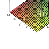
The corresponding scalar curvature can be written as
| (25) |
from which we observe that curvature singularities occur for those values of and that satisfy the equation
| (26) |
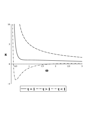
In Fig. 1, we illustrate the behavior of the scalar curvature . The picks on the graph correspond to singularities, i.e., locations where the curvature diverges and the conceptual basis of differential geometry breaks down.
Consider now the GTD metric by assuming in Eq.(7)
| (27) |
which for and reduces to
| (28) |
Furthermore, for the reduced van der Waals fundamental equation (15), we obtain
| (29) |
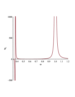
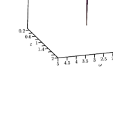
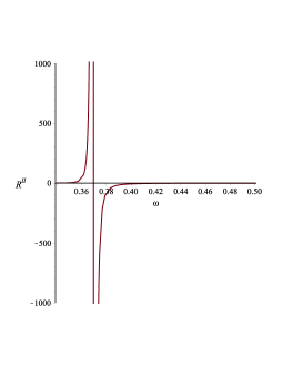
where the function has been defined in Eq.(24). It is then straighforward to compute the scalar curvature, which can be written as
| (30) |
from which it follows that curvature singularities are determined by the equation
| (31) |
The behavior of the curvature scalar is depicted in Fig. 2. For comparison, we choose the same intervals of values for the variables and . The singularity structure can easily be identified and is different from that of the scalar .
Finally, we consider the metric given in Eq.(8), which for and reduces to
| (32) |
Then, for the van der Waals fundamental equation we get
| (33) |
The corresponding curvature cannot be put in a compact form. However, one can show that in general the curvature singularities of the metric are determined by the condition
| (34) |
which is not satisfied by the van der Waals fundamental equation (15).
We conclude that in this case all the information about the curvature singularities of the equilibrium space is contained in the metrics and only.
V Interpretation of the results
According to the formalism of GTD, curvature singularities should indicate the presence of phase transitions. This intuitive idea is based upon the fact that singularities are critical locations at which the concepts of differential geometry cannot be applied anymore, i.e., singularities indicate a break down of the theory of differential geometry. On the other hand, we know that equilibrium thermodynamics breaks down when the system undergoes phase transitions. Based on this analogy, the geometric approaches to thermodynamics consider curvature singularities as the geometric representation of phase transitions. We will show this in the case of van der Waals systems.
V.1 First order phase transitions
First order phase transitions can be detected by considering the isotherms of the reduced pressure (20), which are illustrated in the plots of Fig. 3.
We can see that the behavior of the isotherms depends on the value of and determines the limit between two different classes of isotherms. This is the isotherm for which the temperature coincides with the critical temperature; in Fig. 3, it corresponds to the curve with an inflection point, i.e.,
| (35) |
Then, using the equation of state given in (9), one can show that the inflection point is determined by the solutions of the algebraic equation
| (36) |
which are also interpreted as the points where first order phase transitions occur Callen (1985). This is exactly the condition we have found in Eq.(26) for the existence of curvature singularities of the metric .
V.2 Second order phase transitions
The response functions of a system are used to indicate the presence of second order phase transitions. In the case of a simplet system with two thermodynamic degrees of freedom, there exist only three independent response functions Callen (1985); for concreteness, we choose as independent functions the isothermal compressibility , the thermal expansion at constant pressure , and the heat capacity at constant pressure and temperature , which are defined
| (37) |
Using the relationships: , , and , we obtain the reduced response functions
| (38) |
Furthermore, the reduced response functions can be expressed in terms of the derivatives of the fundamental equation as
| (39) |
Then, substituing the corresponding quantities for a van der Waals system, we obtain
| (40) | |||||
| (41) | |||||
| (42) |
It follows from the above expressions that the response functions diverge if the condition
| (43) |
is satisfied. We recognize immediately that this condition is identical to the condition for the existence of curvature singularities in the equilibrium space of the metric , as given in Eq.(31).
VI Thermodynamic geometry of van der Waals systems
Consider a system described by the fundamental equation . Thermodynamic geometry is an approach based upon the assumption that the geometric properties of the corresponding equilibrium space are determined by a Hessian metric
| (44) |
Although a Hessian metric can be constructed for any function , in thermodynamics only two options have been studied. If the thermodynamic potential is chosen as minus the entropy, , or the internal energy, , the resulting Hessian metrics
| (45) |
are called Ruppeiner Ruppeiner (1979) and Weinhold Weinhold (1975) metrics. We will now investigate the curvature of these metrics in the case of van der Waals systems by using reduced variables.
Using the fundamental equation (15), we obtain
| (46) |
where
| (47) |
and the corresponding curvature scalar reads
| (48) |
Consider now the Weinhold metric. In the energy representation, the fundamental equation (15) can be expressed as
| (49) |
Then, the Weinhold metric can be written explicitly written as
| (50) | |||||
from which we compute the curvature scalar and get
| (51) |
From the above expressions for the curvature scalar it follows that the condition
| (52) |
indicates the presence of singularities in the equilibrium space described by the Ruppeiner and Weinhold metrics. According to the results presented in Sec. V, the curvature of the Hessian metrics can reproduce the first order phase transitions determined by the condition (36), but they are not able to reproduce the second order phase transitions that are predicted by the response functions in Eq.(43).
VII Conclusions
In this work, we tested the formalism of GTD in the case of van der Waals systems. To this end, we first derived the reduced form of the fundamental equation, which has the advantage of being completely general in the sense that it does not depend on the particular values of the van der Waals constants and .
We calculated the scalar curvature of all the three GTD metrics in order to find the locations where curvature singularities can exist. This analysis lead to the conclusion that there are two different conditions that indicate the presence of singularities. By analyzing the thermodynamic properties of van der Waals systems we proved that the locations of the curvature singularities coincide with the points at which first and second order phase transitions occur. This shows that GTD can describe the entire phase transition structure of van der Waals systems.
Moreover, we investigated the properties of the equilibrium space as defined in thermodynamic geometry by means of Hessian metrics. We found that this approach correctly predicts the presence of first order phase transitions only.
The results presented in this work can be applied to any system characterized by two thermodynamic degrees of freedom. The formalism of GTD is completely general, although the explicit form of the GTD metrics depend on the fundamental equation of the corresponding system. We thus conclude that to study the equilibrium space and the complete phase transition structure of any thermodynamic system in an invariant way, one can use the metrics obtained in the framework of the GTD formalism.
Acknowledgments
This work was carried out within the scope of the project CIAS 3131 supported by the Vicerrectoría de Investigaciones de la Universidad Militar Nueva Granada - Vigencia 2020. This work was partially supported by UNAM-DGAPA-PAPIIT, Grant No. 114520, Conacyt-Mexico, Grant No. A1-S-31269, and by the Ministry of Education and Science of RK, Grant No. BR05236322 and AP05133630.
References
- Frankel (2004) T. Frankel, The Geometry of Physics: An Introduction (Cambridge University Press, 2004).
- Rao (1945) C. R. Rao, Bulletin of Calcutta Mathematical Society 37, 81 (1945).
- Amari (2012) S. Amari, Differential-Geometrical Methods in Statistics, Lecture Notes in Statistics (Springer New York, 2012).
- Weinhold (1975) F. Weinhold, The Journal of Chemical Physics 63, 2479 (1975).
- Ruppeiner (1979) G. Ruppeiner, Physical Review A 20, 1608 (1979).
- Ruppeiner (1995) G. Ruppeiner, Reviews of Modern Physics 67, 605 (1995).
- Quevedo (2007) H. Quevedo, Journal of Mathematical Physics 48, 013506 (2007).
- Callen (1985) H. B. Callen, Thermodynamics and an introduction to thermostatistics; 2nd ed. (Wiley, New York, NY, 1985).
- Weinhold (2009) F. Weinhold, Classical and geometrical theory of chemical and phase thermodynamics (John Wiley & Sons, 2009).
- Ruppeiner (2014) G. Ruppeiner, in Breaking of Supersymmetry and Ultraviolet Divergences in Extended Supergravity (Springer, 2014) pp. 179–203.
- Åman et al. (2015) J. E. Åman, I. Bengtsson, and N. Pidokrajt, Entropy 17, 6503 (2015).
- Mandal and Biswas (2015) A. Mandal and R. Biswas, Astrophysics and Space Science 357, 1 (2015).
- Bravetti and Luongo (2014) A. Bravetti and O. Luongo, International Journal of Geometric Methods in Modern Physics 11, 1450071 (2014).
- Hendi et al. (2016) S. Hendi, S. Panahiyan, and B. E. Panah, Journal of High Energy Physics 2016, 1 (2016).
- Kubizňák and Mann (2015) D. Kubizňák and R. B. Mann, Canadian Journal of Physics 93, 999 (2015).
- Arnold (1989) V. Arnold, Mathematical methods of classical mechanics, Vol. 60 (Springer, 1989).
- Alberty (1994) R. A. Alberty, Chemical Reviews 94, 1457 (1994), https://doi.org/10.1021/cr00030a001 .
- Quevedo et al. (2018) H. Quevedo, M. N. Quevedo, and A. Sánchez, The European Physical Journal C 79, 1 (2018).
- Greiner et al. (2012) W. Greiner, L. Neise, and H. Stöcker, Thermodynamics and statistical mechanics (Springer Science & Business Media, 2012).
- Huang (2009) K. Huang, Introduction to statistical physics (Chapman and Hall/CRC, 2009).
- Reif (2009) F. Reif, Fundamentals of statistical and thermal physics (Waveland Press, 2009).