Stability of $d$-dimensional Gravastars with Variable Equation of State

Abstract

In this paper, we are interested to explore stable configurations of $d$-dimensional gravastars constructed from the interior $d$-dimensional de Sitter and exterior $d$-dimensional Schwarzschild/Reissner-Nordström (de Sitter) black holes through cut and paste approach. We consider the linearized radial perturbation preserving the original symmetries to explore their stability by using three different types of matter distributions. The resulting frameworks represent unstable structures for barotropic, Chaplygin, and phantomlike models for every considered choice of exterior geometries. However, matter contents with variable equations of state have a remarkable role to maintain the stability of gravastars. We conclude that stable structures of gravastars are obtained only for generalized variable models with exterior $d$-dimensional Schwarzschild/Reissner-Nordström-de Sitter black holes.

Keywords: Gravastars; Black holes; Equation of state; Stability.
PACS: 04.20.-q; 04.70.Dy; 04.40.Dg; 04.50.Gh.

1 Introduction

A decade or more ago, Mazur and Mottola [1, 2] proposed a new solution for the endpoint of a gravitational collapse. They developed a cold compact object composed of an interior de Sitter (dS) and exterior Schwarzschild geometry by applying the principle of Bose-Einstein condensation to gravitational structures. These geometries are partitioned by a phase boundary having a small and finite thickness ($r_{i}-r_{o}=\delta$) which is also referred to as thin-shell, where the inner and outer radii of gravastar are denoted by $r_{i}$ and $r_{o}$, respectively. Consequently, the matter distributions at these sections can be characterized through some specific equations of state (EoS) given as

• Inner manifold: $0\leq r<r_{i}$, $p=-\sigma$,

• Thin-shell: $r_{i}<r<r_{o}$, $p=\sigma$,

• Outer manifold: $r_{o}<r$, $p=0=\sigma$.

The surface energy density and pressure of the matter contents are represented by $\sigma$ and $p$, respectively. To achieve a stable configuration, the concentration of matter at thin-shell plays a vital role to overcome the rapidly expanding and collapsing nature of thin-shell. The cut and paste technique [3] offers a general formalism for thin-shell construction from the matching of two distinct spacetimes at hypersurface. This formalism is used to construct thin-shell gravastar from the matching of interior dS and external Schwarzschild BH [2]. This method is very useful in avoiding the existence of central singularity and event horizon in the developed geometrical structure. We have also studied thin-shell stability as well as dynamics developed from cut and paste approach [4, 5].

Gravastars have attracted many researchers to study their basic framework using various methods. Visser and Wiltshire [6] discussed stable characteristics of gravastars by introducing different EoS. Horvat and Ilijic [7] studied gravastar model with exterior Schwarzschild and Schwarzschild-dS geometries. This formalism is extended for inner dS and outer Reissner-Nordström (RN) BH in [8, 9]. The physical characteristics like length, energy contents, and entropy of (2+1)-dimensional charged free and charged gravastars are investigated in [10]. The charged gravastar model with interior dS and exterior RN-dS spacetime is constructed in [11].

The study of the possible existence of bounded excursion gravastars (in which shell radius oscillates between two radii) is an interesting topic in the background of different exterior geometries. The prototype gravastar model was introduced by Rocha and his collaborators [12] by using external Schwarzschild BH and internal dS spacetime with stiff as well as dust fluid distributions. They analyzed that the developed structure expresses stable bounded excursion gravastars or collapsing behavior until BHs are formed. Thus, in such complex models, the probability of the existence of a gravastar model cannot be eliminated. This analysis was also extended for inner dS and outer Schwarzschild-dS and RN BHs in [13, 14]. It is found that the presence of a cosmological constant in the exterior geometry leads to a stable configuration of gravastar [13].

The stability of the gravastar model with a different type of matter distribution through linearized radial perturbation is also an interesting issue. Lobo and Arellano [15] constructed thin-shell gravastars with nonlinear electrodynamics. The stable configuration of noncommutative thin-shell gravastar is investigated by Lobo and Garattini [16]. They noticed that stable regions must exist near the predicted location of the event horizon. Övgün et al. [17] investigated the stability of gravastars constructed from the interior dS and exterior charged noncommutative BHs. They concluded that the developed structure shows stable behavior near the formation of the event horizon for suitable values of the physical parameters. Recently, we have constructed thin-shell gravastar from exterior regular as well as charged Kiselve BHs and explored the stability of the developed geometry through radial perturbation by considering variable EoS [18].

A significant subject in general relativity and modified gravity theories is the study of gravastars in higher dimensions. The class of gravastar solutions as an alternative to $d$-dimensional BHs are presented in [19]-[21]. A fascinating type of traversable wormhole is the thin-shell kind, which is built by grafting two equivalent manifolds together to form a geodesically complete spacetime with a shell positioned at the junction interface. Dias and Lemos [22] constructed $d$-dimensional electrically charged thin-shell wormholes and observed their stability. Eiroa and Simeone [23] studied the stability of $d$-dimensional static shells through spherically symmetric radial perturbation and found that stable regions are increased for higher dimensions. The stable configurations of $d$-dimensional thin-shell surrounded by quintessence through linearized radial perturbation are analyzed in [24] and its dynamics with massless and massive scalar fields are observed in [25].

In this paper, we study the stability of higher-dimensional gravastars by taking as an alternative to $d$-dimensional Schwarzschild, Schwarzschild-dS, RN and RN-dS BHs. The paper is organized in the following format. Section 2 is devoted to construct $d$-dimensional gravastars and consider Lanczos equations to obtain matter contents of thin-shell. Section 3 is used to discuss the stability of the developed structure filled with barotropic and generalized variable EoS. We observe the stability of gravastars for different $d$-dimensional BHs. In the last section, we briefly discuss the outcomes.

2 Geometry of $d$-Dimensional Gravastars

We consider Israel thin-shell formalism for smooth matching of the interior $d$-dimensional dS spacetime with different exterior $d$-dimensional BH geometries at the hypersurface. We develop the mathematical expression of the equation of motion of gravastar by using Lanczos equations. This equation plays a vital role to express the dynamical as well as stable configurations of the established frameworks in the presence of different types of matter distributions.

2.1 Interior Geometry

In general relativity, the dS geometry serves as the simplest mathematical model which explains the physics of the current scenario associated with the observed accelerated expansion of the universe. It is a vacuum solution of the field equations with negative pressure and positive vacuum energy density. The universe itself behaves as asymptotically dS with cosmological confirmations. The $d$-dimensional dS spacetime is a Lorentzian manifold having maximum symmetrical configurations with positive scalar constant curvature and is an analog of a $d$-sphere. The line element of the $d$-dimensional dS spacetime can be written as [26]

$$ds^{2}_{-} = -\mathcal{H}(r_{-})dt^{2}_{-}+\mathcal{H}(r_{-})^{-1}dr^{2}_{-}+r^{2}_{-}d\Omega^{2}_{d-2},$$ (1)

where the line element of $(d-2)$ unit sphere is denoted by $d\Omega^{2}_{d-2}$ and its metric function is given as

$$\mathcal{H}(r_{-})=1-\frac{r^{2}_{-}}{L_{i}^{2}},\quad\text{with}\quad L_{i}=\sqrt{\frac{(d-1)(d-2)}{2\Lambda_{i}}},$$

here $\Lambda_{i}$ represents the cosmological constant and cosmological event horizon at $r_{c-}=\alpha$. For different choices of $\Lambda_{i}$, it leads to different spacetimes, i.e., dS for $\Lambda_{i}>0$, anti dS (AdS) for $\Lambda_{i}<0$ and flat region for $\Lambda_{i}=0$.

2.2 Exterior Geometry

To construct $d$-dimensional gravastar, we consider the exterior spacetime as a $d$-dimensional BH. The line element of this spacetime is [26]

$$ds^{2}_{+} = -\mathcal{F}(r_{+})dt^{2}_{+}+\mathcal{F}(r_{+})^{-1}dr^{2}_{+}+r^{2}_{+}d\Omega^{2}_{d-2}.$$ (2)

Different choices of the metric function ($\mathcal{F}(r_{+})$) leads to different BHs.

• For $d$-dimensional Schwarzschild BH, it can be expressed as

  $$\mathcal{F}(r_{+})=1-\frac{2m}{r^{d-3}_{+}},$$

  where $m$ is the mass of BH.

• For $d$-dimensional Schwarzschild-dS BH, it yields

  $$\mathcal{F}(r_{+})=1-\frac{2m}{r^{d-3}_{+}}-\frac{r^{2}_{+}}{L_{e}^{2}},\quad\text{with}\quad L_{e}=\sqrt{\frac{(d-1)(d-2)}{2\Lambda_{e}}},$$

  where $\Lambda_{e}$ represents the cosmological constant of exterior geometry.

• For $d$-dimensional RN BH, it turns out to be

  $$\mathcal{F}(r_{+})=1-\frac{2m}{r^{d-3}_{+}}+\frac{Q^{2}}{r^{2(d-3)}_{+}},$$

  where $Q$ is the charge distribution of the BH spacetime.

• For $d$-dimensional RN-dS BH, it becomes

  $$\mathcal{F}(r_{+})=1-\frac{2m}{r^{d-3}_{+}}+\frac{Q^{2}}{r^{2(d-3)}_{+}}-\frac{r^{2}_{+}}{L_{e}^{2}}.$$

2.3 Visser Cut and Paste Approach

Visser’s approach is the best mathematical technique to construct a geometrical structure free from event horizons and singularities through the joining of inner and outer spacetimes. We apply this technique to obtain the geometrical structure of $d$-dimensional gravastar. For this purpose, we match these spacetimes at the timelike hypersurface ($\Sigma$) which is also known as $(d-1)$-dimensional spacetime. The hypersurface is referred to as a gravastar shell with radius $r=y(\tau)\equiv y$, where $\tau$ is the proper time. To avoid the event horizons and singularities in the developed structure, the shell radius $y$ must be greater than the event horizons of the considered spacetimes. According to Israel junction conditions, the line element of a hypersurface, inner and outer manifolds are identical, i.e., $ds^{2}_{-}\cong ds^{2}_{\Sigma}\cong ds^{2}_{+}$. The corresponding line elements (1) and (2) of inner and outer manifolds at $r_{+}=r_{-}=y$ can be expressed as

$$ds^{2}_{-} = \left[-\mathcal{H}(y)+\mathcal{H}(y)^{-1}(dy/d\tau)^{2}(d\tau/dt)^{2}\right]dt^{2}+y^{2}d\Omega^{2}_{d-2},$$ (3)

$$ds^{2}_{+} = \left[-\mathcal{F}(y)+\mathcal{F}(y)^{-1}(dy/d\tau)^{2}(d\tau/dt)^{2}\right]dt^{2}+y^{2}d\Omega^{2}_{d-2}.$$ (4)

The line element of the hypersurface is given as

$$ds^{2}_{\Sigma}=-d\tau^{2}+y^{2}d\Omega^{2}_{d-2},$$ (5)

The proper time derivative of temporal coordinate is obtained by comparing Eq.(5) with Eqs.(3) and (4). Hence, we have

$$dt/d\tau=\dot{t}=\begin{cases}(\mathcal{H}(y)+\dot{y}^{2})^{1/2}/\mathcal{H}(y),\quad\text{for the interior region}\\ (\mathcal{F}(y)+\dot{y}^{2})^{1/2}/\mathcal{F}(y),\quad\text{for the exterior region.}\end{cases}$$ (6)

The second Israel junction condition demonstrates discontinuity of the extrinsic curvature at $\Sigma$, i.e., $[K^{a}_{b}]=K^{a}_{b(i)}-K^{a}_{b(e)}\neq 0$. The matching of considered spacetimes leads to the boundary surface if $[K^{a}_{b}]=0$, otherwise it shows the existence of thin-shell. The extrinsic curvature components can be defined as

$$K_{ij}^{\pm}=-n_{\beta}^{\pm}\left(\frac{d^{2}y_{\pm}^{\beta}}{d\xi^{i}d\xi^{j}}+\Gamma^{\beta\pm}_{\mu\nu}\frac{dy^{\mu}_{\pm}}{d\xi^{i}}\frac{dy^{\nu}_{\pm}}{d\xi^{j}}\right),\quad i,j=0,2,3,\dotso,d,$$ (7)

where $\xi^{i}$ denotes hypersurface coordinates and the outward unit normals to the considered manifolds are given as

$$n_{\alpha}^{-} = \pm\mid g^{\mu\nu}\frac{\partial\mathcal{H}(y)}{\partial y^{\mu}}\frac{\partial\mathcal{H}(y)}{\partial y^{\nu}}\mid^{-\frac{1}{2}}\frac{\partial\mathcal{H}(y)}{\partial y^{\alpha}},\quad\alpha=0,1,2,\dotso,d,$$

$$n_{\alpha}^{+} = \pm\mid g^{\mu\nu}\frac{\partial\mathcal{F}(y)}{\partial y^{\mu}}\frac{\partial\mathcal{F}(y)}{\partial y^{\nu}}\mid^{-\frac{1}{2}}\frac{\partial\mathcal{F}(y)}{\partial y^{\alpha}}.$$

The corresponding $(t,t)$ and $(\theta,\theta)$ components of extrinsic curvature become

$$K^{\tau}_{\tau} = \begin{cases}(\mathcal{H}^{\prime}(y)+2\ddot{y}^{2})/(\mathcal{H}(y)+\dot{y}^{2})^{1/2},\quad\text{for interior region}\\ (\mathcal{H}^{\prime}(y)+2\ddot{y}^{2})/(\mathcal{F}(y)+\dot{y}^{2})^{1/2},\quad\text{for exterior region}\end{cases}$$ (8)

$$K^{\theta}_{\theta} = \begin{cases}(\mathcal{H}(y)+\dot{y}^{2})^{1/2}/y,\quad\text{for interior region}\\ (\mathcal{F}(y)+\dot{y}^{2})^{1/2}/y,\quad\text{for exterior region}\end{cases}$$ (9)

where dash represents derivative to the shell radius $y$.

The discontinuity of extrinsic curvature is due to the presence of a thin layer of matter surface at $\Sigma$. Such type of matter distribution greatly affects the dynamics and stability of the established frameworks. The stress-energy tensor components of matter contents can be evaluated through the reduced form of the field equations at $\Sigma$. These equations are known as Lanczos equations and are given as

$$8\pi S_{i}^{j}=\delta_{i}^{j}K-[K_{i}^{j}],$$ (10)

where $S_{i}^{j}$ represents the stress-energy tensor and $\delta_{i}^{j}$ is known as the Kronecker delta. The stress-energy tensor for perfect fluid has the form

$$S_{i}^{j}=v_{i}v^{j}\left(\rho+p\right)+\delta^{j}_{i}p,$$ (11)

where $v_{i}$, $\rho$ and $p$ represent the shell velocity, energy density and surface pressure of thin layer of matter at $\Sigma$, respectively. For the considered manifolds, the Lanczos equations can be expressed as

$$\rho(y) = -\frac{d-2}{8\pi y}\left\{\sqrt{\dot{y}^{2}+\mathcal{F}(y)}-\sqrt{\dot{y}^{2}+\mathcal{H}(y)}\right\},$$ (12)

$$p(y) = \frac{1}{8\pi y}\left\{\frac{y\mathcal{F}^{\prime}(y)+2y\ddot{y}+2(d-3)\left(\dot{y}^{2}+\mathcal{F}(y)\right)}{\sqrt{\dot{y}^{2}+\mathcal{F}(y)}}\right.$$ (13)

$$- \left.\frac{y\mathcal{H}^{\prime}(y)+2y\ddot{y}+2(d-3)\left(\dot{y}^{2}+\mathcal{H}(y)\right)}{\sqrt{\dot{y}^{2}+\mathcal{H}(y)}}\right\}.$$

It is noted that the shell does not move at equilibrium shell radius $y=y_{0}$ in the radial direction. Hence, the proper time derivative of shell radius at $y=y_{0}$ vanishes, i.e., $\dot{y}_{0}=0=\ddot{y}_{0}$. The corresponding expressions of energy density and surface pressure at $y=y_{0}$, yield

$$\rho(y_{0}) = -\frac{d-2}{8\pi y_{0}}\left\{\sqrt{\mathcal{F}(y_{0})}-\sqrt{\mathcal{H}(y_{0})}\right\},$$ (14)

$$p(y_{0}) = \frac{y_{0}\mathcal{F}^{\prime}(y_{0})+2(d-3)\mathcal{F}(y_{0})}{8\pi y_{0}\sqrt{\mathcal{F}(y_{0})}}-\frac{y_{0}\mathcal{H}^{\prime}(y_{0})+2(d-3)\mathcal{H}(y_{0})}{8\pi y_{0}\sqrt{\mathcal{H}(y_{0})}}.$$ (15)

The equation of motion of the shell can be obtained from Eq.(12) as

$$\frac{1}{2}\dot{y}^{2}+\Pi(y)=0,$$ (16)

where

$$\Pi(y) = -\frac{8\pi^{2}y^{2}\sigma^{2}}{(d-2)^{2}}-\frac{(d-2)^{2}\mathcal{Z}^{2}(y)}{512\pi^{2}y^{2}\sigma^{2}}+\frac{\mathcal{W}(y)}{4},$$ (17)

and the functions $\mathcal{Z}(y)$ and $\mathcal{W}(y)$ are defined as

$$\mathcal{Z}(y)=\mathcal{H}(y)-\mathcal{F}(y),\quad\mathcal{W}(y)=\mathcal{H}(y)+\mathcal{F}(y).$$

3 Stability Analysis

In this section, we discuss the stability of the developed structure by using linearized radial perturbation. We consider three different choices of matter distributions, i.e., barotropic EoS, generalized Chaplygin variable (GCV) and generalized phantomlike variable (GPV) models. The last two models depending on the shell radius of the developed structure are also known as variable EoS. We develop respective expressions of the effective potential of gravastar for these EoS. We then explore the behavior of effective potential to observe the final fate of the developed structure. It is mentioned here that the behavior of gravastar geometry (stable and unstable configurations) can be evaluated through the graphical behavior of effective potential. If the potential function and its first derivative vanish at $y=y_{0}$, then it shows stable behavior for $\Pi^{\prime\prime}(y_{0})>0$, unstable structure if $\Pi^{\prime\prime}(y_{0})<0$ and unpredictable if $\Pi^{\prime\prime}(y_{0})=0$ [28]. We use linear radial perturbation of the effective potential about equilibrium shell radius up to second-order terms to explore the stable configurations.

The Taylor series of $\Pi(y)$ about $y=y_{0}$ is given as

$$\Pi(y)=\Pi(y_{0})+\Pi^{\prime}(y_{0})(y-y_{0})+\frac{1}{2}\Pi^{\prime\prime}(y_{0})(y-y_{0})^{2}+O[(y-y_{0})^{3}].$$

It is found that $\Pi(y_{0})=0=\Pi^{\prime}(y_{0})$, hence the above equation becomes

$$\Pi(y)=\frac{1}{2}(y-y_{0})^{2}\Pi^{\prime\prime}(y_{0}).$$ (18)

The relation between surface stresses of thin-shell can be determined through the conservation equation as

$$4\pi\frac{d}{d\tau}(y^{2}\sigma)+4\pi p(\sigma,y)\frac{dy^{2}}{d\tau}=0,$$ (19)

which can be written as

$$\frac{d\sigma}{dy}=-\frac{2}{y}(\sigma+p(\sigma,y)).$$ (20)

The derivative of the above equation with respect to the shell radius becomes

$$\frac{d^{2}\sigma}{dy^{2}}=\frac{p(\sigma,y)+\sigma}{y^{2}}\left(2+\vartheta^{2}\right),$$ (21)

where the EoS parameter can be expressed as $\vartheta^{2}=dp/d\sigma$.

To investigate stability, we choose a specific expression of $p(\sigma,y)$ which leads to different types of matter distributions. We begin with linear EoS, $p=\eta\sigma$, where $\eta$ is the barotropic EoS parameter. This gives a linear relationship between surface energy density and pressure of matter contents located at thin-shell. The corresponding solution of the conservation equation (20) yields

$$\sigma=\left(y_{0}/y\right)^{2(1+\eta)}\sigma_{0}.$$ (22)

The respective expression of $\Pi(y)$ turns out to be

$$\Pi(y)=\frac{1}{4}\mathcal{W}(y)-\frac{(d-2)^{2}\mathcal{Z}(y)^{2}}{512\pi^{2}y^{2}\sigma_{0}^{2}}\left(\frac{y_{0}}{y}\right)^{-4(\eta+1)}-\frac{8\pi^{2}y^{2}\sigma_{0}^{2}}{(d-2)^{2}}\left(\frac{y_{0}}{y}\right)^{4(\eta+1)}.$$ (23)

It is found that $\Pi(y_{0})=0$ and $\Pi^{\prime}(y_{0})$ can be written as

$$\Pi^{\prime}(y_{0}) = \frac{16\pi^{2}y_{0}\sigma_{0}^{2}}{(d-2)^{2}}(2\eta+1)-\frac{(d-2)^{2}\mathcal{Z}(y_{0})}{256\pi^{2}\sigma_{0}^{2}y_{0}^{3}}\left(2\eta\mathcal{Z}(y_{0})+y_{0}\mathcal{Z}^{\prime}(y_{0})+\mathcal{Z}(y_{0})\right)$$

$$+ \frac{\mathcal{W}^{\prime}(y_{0})}{4},$$

which vanishes only if

$$\eta=\frac{\frac{(d-2)^{2}\mathcal{Z}(y_{0})^{2}}{256\pi^{2}\sigma_{0}^{2}y_{0}^{3}}+\frac{(d-2)^{2}\mathcal{Z}(y_{0})\mathcal{Z}^{\prime}(y_{0})}{256\pi^{2}\sigma_{0}^{2}y_{0}^{2}}-\frac{16\pi^{2}\sigma_{0}^{2}y_{0}}{(d-2)^{2}}-\frac{\mathcal{W}^{\prime}(y_{0})}{4}}{\frac{32\pi^{2}\sigma_{0}^{2}y_{0}}{(d-2)^{2}}-\frac{(d-2)^{2}\mathcal{Z}(y_{0})^{2}}{128\pi^{2}\sigma_{0}^{2}y_{0}^{3}}}.$$ (24)

Hence, we have

$$\Pi^{\prime\prime}(y_{0}) = -\left(-64\pi^{2}\sigma_{0}^{2}y_{0}^{4}\left((d-2)^{2}\mathcal{W}^{\prime\prime}(y_{0})-64\pi^{2}\sigma_{0}^{2}(2\eta+1)(4\eta+3)\right)\right.$$ (25)

$$+ \left.(d-2)^{4}\left(8\eta^{2}+6\eta+1\right)\mathcal{Z}(y_{0})^{2}+(d-2)^{4}y_{0}\mathcal{Z}(y_{0})\left(y_{0}\mathcal{Z}^{\prime\prime}(y_{0})\right.\right.$$

$$+ \left.\left.(8\eta+4)\mathcal{Z}^{\prime}(y_{0})\right)+(d-2)^{4}y_{0}^{2}\mathcal{Z}^{\prime}(y_{0})^{2}\right)$$

$$\times (256\pi^{2}(d-2)^{2}\sigma_{0}^{2}y_{0}^{4})^{-1}.$$

This equation is used to explore the stable/unstable geometrical configurations of thin-shell gravastars filled with the barotropic type fluid distributions.

We also obtain dynamical equations of the developed configurations filled with fluid distribution for GCV EoS given as $p=\frac{1}{y^{n}}\frac{\beta}{\sigma}$, where $\beta$ and $n$ are the real constants [27, 28], for $n=0$, the Chaplygin gas model is recovered [29]. The corresponding solution is

$$\sigma^{2}=\frac{(n-4)\sigma_{0}^{2}y_{0}^{n+4}y^{n}+4\beta y^{4}y_{0}^{n}-4\beta y^{n}y_{0}^{4}}{y^{n+4}y_{0}^{n}(n-4)}.$$ (26)

Consequently, the effective potential leads to

$$\Pi(y) = \frac{1}{4}\mathcal{W}(y)-\frac{(d-2)^{2}}{512\pi^{2}}\frac{(n-4)y^{n+2}\mathcal{Z}(y)^{2}y_{0}^{n}}{\left(y_{0}^{4}y^{n}\left((n-4)\sigma_{0}^{2}y_{0}^{n}-4\beta\right)+4y^{4}\beta y_{0}^{n}\right)}$$ (27)

$$- \frac{8\pi^{2}y^{-n-2}y_{0}^{-n}}{(d-2)^{2}(n-4)}\left(y_{0}^{4}y^{n}\left((n-4)\sigma_{0}^{2}y_{0}^{n}-4\beta\right)+4y^{4}\beta y_{0}^{n}\right).$$

At equilibrium shell radius, the effective potential vanishes and its first derivative with respect to shell radius is given as

$$\Pi^{\prime}(y_{0}) = \left(-2(d-2)^{4}\beta\mathcal{Z}(y_{0})^{2}-(d-2)^{2}\sigma_{0}^{2}y_{0}^{n}\left((d-2)^{2}\mathcal{Z}(y_{0})\left(y_{0}\mathcal{Z}^{\prime}(y_{0})\right.\right.\right.$$

$$+ \left.\left.\left.\mathcal{Z}(y_{0})\right)-64\pi^{2}\sigma_{0}^{2}y_{0}^{3}\mathcal{W}^{\prime}(y_{0})\right)+4096\pi^{4}\sigma_{0}^{4}y_{0}^{4}\left(2\beta+\sigma_{0}^{2}y_{0}^{n}\right)\right)$$

$$\times (256y^{n+3}_{0}\pi^{2}(d-2)^{2}\sigma_{0}^{4})^{-1}.$$

For $\Omega^{\prime}(y_{0})=0$, we obtain

$$\beta = \frac{-\sigma_{0}^{2}y_{0}^{n}}{8192\pi^{4}\sigma_{0}^{4}y_{0}^{4}-2(d-2)^{4}\mathcal{Z}(y_{0})^{2}}\left(64\pi^{2}\sigma_{0}^{2}y_{0}^{3}\left((d-2)^{2}\mathcal{W}^{\prime}(y_{0})\right.\right.$$ (28)

$$+ \left.\left.64\pi^{2}\sigma_{0}^{2}y_{0}\right)+(d-2)^{4}(-y_{0})\mathcal{Z}(y_{0})\mathcal{Z}^{\prime}(y_{0})-(d-2)^{4}\mathcal{Z}(y_{0})^{2}\right),$$

and

$$\Pi^{\prime\prime}(y_{0}) = \frac{y_{0}^{-2(n+2)}}{256\pi^{2}(d-2)^{2}\sigma_{0}^{6}}\left(-(d-2)^{4}\mathcal{Z}(y_{0})^{2}\left(16\beta^{2}-2\beta(n-7)\sigma_{0}^{2}y_{0}^{n}\right.\right.$$ (29)

$$+ \left.\left.\sigma_{0}^{4}y_{0}^{2n}\right)-(d-2)^{4}\sigma_{0}^{2}y_{0}^{n+1}\mathcal{Z}(y_{0})\left(8\sigma_{0}\mathcal{Z}^{\prime}(y_{0})+\sigma_{0}^{2}y_{0}^{n}\left(y_{0}\mathcal{Z}^{\prime\prime}(y_{0})\right.\right.\right.$$

$$+ \left.\left.\left.4\mathcal{Z}^{\prime}(y_{0})\right)\right)+64\pi^{2}\sigma_{0}^{6}y_{0}^{n+4}\left((d-2)^{2}y_{0}^{n}\mathcal{W}^{\prime\prime}(y_{0})-64\pi^{2}\left(2\beta(n+1)\right.\right.\right.$$

$$+ \left.\left.\left.3\sigma_{0}^{2}y_{0}^{n}\right)\right)-(d-2)^{4}\sigma_{0}^{4}y_{0}^{2n+2}\mathcal{Z}^{\prime}(y_{0})^{2}\right).$$

This is used to analyze stability of thin-shell gravastars filled with matter which follows GCV EoS.

Finally, we take GPV EoS, i.e., $p=\frac{\lambda\sigma}{y^{n}}$, where $\lambda$ and $n$ are real constants [27, 28]. For $n=0$, phantomlike EoS is obtained [30]. The respective solution of conservation equation gives

$$\sigma=y_{0}^{2}y^{-2}\sigma_{0}e^{\frac{\lambda\left(y_{0}^{-n}-y^{-n}\right)}{n}},$$ (30)

and it follows that

$$\Pi(y)=\frac{1}{4}\mathcal{W}(y)-\frac{y^{2}(d-2)^{2}\mathcal{Z}(y)^{2}}{512\pi^{2}\sigma_{0}y_{0}^{4}}e^{\frac{2\lambda\left(y_{0}^{-n}-y^{-n}\right)}{n}}-\frac{8\pi^{2}\sigma_{0}}{y_{0}^{-4}y^{2}}\frac{e^{\frac{2\lambda\left(y^{-n}-y_{0}^{-n}\right)}{n}}}{(d-2)^{2}}.$$ (31)

Also, we have

$$\Pi^{\prime}(y_{0}) = \frac{y_{0}^{-n-3}(d-2)^{-2}}{256\pi^{2}\sigma_{0}}\left(64\pi^{2}\sigma_{0}y_{0}^{3}\left(64\pi^{2}\sigma_{0}y_{0}\left(\lambda+y_{0}^{n}\right)+(d-2)^{2}y_{0}^{n}\mathcal{W}^{\prime}(y_{0})\right.\right.$$

$$- \left.\left.(d-2)^{4}y_{0}^{n+1}\mathcal{Z}(y_{0})\mathcal{Z}^{\prime}(y_{0})\right)-(d-2)^{4}\mathcal{Z}(y_{0})^{2}\left(\lambda+y_{0}^{n}\right)\right).$$

It is found that $\Pi(y_{0})=0$ and by taking $\Pi^{\prime}(y_{0})=0$, we obtain

$$\lambda = y_{0}^{n}\left(-64\pi^{2}\sigma_{0}y_{0}^{3}\left((d-2)^{2}\mathcal{W}^{\prime}(y_{0})+64\pi^{2}\sigma_{0}y_{0}\right)+(d-2)^{4}y_{0}\mathcal{Z}(y_{0})\mathcal{Z}^{\prime}(y_{0})\right.$$

$$+ \left.(d-2)^{4}\mathcal{Z}(y_{0})^{2}\right)\left(4096\pi^{4}\sigma_{0}^{2}y_{0}^{4}-(d-2)^{4}\mathcal{Z}(y_{0})^{2}\right)^{-1},$$

and hence

$$\Pi^{\prime\prime}(y_{0}) = \frac{y_{0}^{-2(n+2)}\pi^{-2}}{256(d-2)^{2}\sigma_{0}}\left(-(d-2)^{4}y_{0}^{2n+2}\mathcal{Z}^{\prime}(y_{0})^{2}-(d-2)^{4}\mathcal{Z}(y_{0})^{2}\left(2\lambda^{2}\right.\right.$$ (32)

$$- \left.\left.\lambda(n-3)y_{0}^{n}+y_{0}^{2n}\right)+64\pi^{2}\sigma_{0}y_{0}^{4}\left((d-2)^{2}y_{0}^{2n}\mathcal{W}^{\prime\prime}(y_{0})\right.\right.$$

$$- \left.\left.64\pi^{2}\sigma_{0}\left(2\lambda^{2}+\lambda(n+5)y_{0}^{n}+3y_{0}^{2n}\right)\right)-(d-2)^{4}y_{0}^{n+1}\mathcal{Z}(y_{0})\left(4\left(\lambda\right.\right.\right.$$

$$+ \left.\left.\left.y_{0}^{n}\right)\mathcal{Z}^{\prime}(y_{0})+y_{0}^{n+1}\mathcal{Z}^{\prime\prime}(y_{0})\right)\right).$$

In the following, we study the influence of physical parameters on the stability of the structure through graphs.

3.1 Different Choices of Exterior Geometries

We are interested to explore the stability of the developed structure in the background of different choices of exterior BH spacetimes, i.e., $d$-dimensional Schwarzschild (dS) and RN (dS) spacetimes. The possible existence of stable bounded excursion gravastars for these exterior geometries have been explored in four-dimensional spacetimes [12]-[14]. We develop the respective equations of motion of thin-shell filled with barotropic, GCV, and GPV EoS. We use a graphical approach to discuss the second derivative of the effective potential for suitable values of physical parameters. The stable characteristics of gravastar for different values of $d$ are shown in Figures 1-12. Here, we use $d=4$ (blue), $d=6$ (red), $d=8$ (brown), $d=10$ (green).

3.1.1 $d$-dimensional Schwarzschild BH

In the background of $d$-dimensional Schwarzschild BH, we have

$$\mathcal{Z}(y) = 2my^{3-d}-\frac{2y^{2}\Lambda_{i}}{(d-2)(d-1)},$$

$$\mathcal{W}(y) = -\frac{2y^{2}\Lambda_{i}}{(d-2)(d-1)}-2my^{3-d}+2.$$

Using the above expressions in Eqs.(25), (29) and (32), we obtain $\Pi^{\prime\prime}(y_{0})$ for $d$-dimensional Schwarzschild BH and thin-shell filled with matter satisfying barotropic, GCV and GPV EoS, respectively. The developed structure represents the unstable configuration for every choice of fluid distributions as shown in Figures 1-3. This shows that the choice of interior $d$-dimensional dS and exterior $d$-dimensional Schwarzschild BH leads to an unstable structure of gravastar.

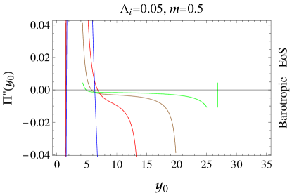
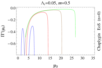
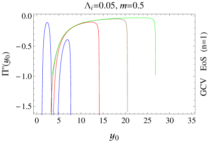
Figure 1: Unstable configuration of $d$-dimensional gravastar for barotropic EoS with exterior $d$-dimensional Schwarzschild BH. The blue, red, brown and green colors represent the behavior of $\Pi^{\prime\prime}(y_{0})$ for $d=4,6,8,10$, respectively. It is noted that the developed structure shows unstable configuration as $\Pi^{\prime\prime}(y_{0})<0$ for every choice of physical parameter.

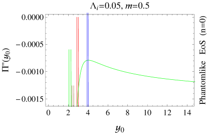
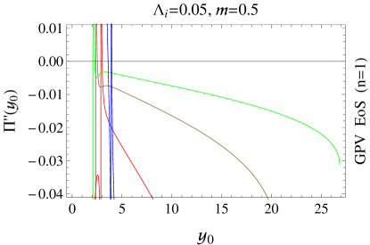
Figure 2: Unstable configuration of $d$-dimensional gravastar for Chaplygin and GCV EoS with exterior $d$-dimensional Schwarzschild BH.

Figure 3: Unstable configuration of $d$-dimensional gravastar for phantomlike and GPV EoS with exterior $d$-dimensional Schwarzschild BH.

3.1.2 $d$-dimensional Schwarzschild-dS BH

For $d$-dimensional Schwarzschild-dS BH, it follows that

$$\mathcal{Z}(y) = \frac{2y^{2}\Lambda_{e}}{(d-2)(d-1)}-\frac{2y^{2}\Lambda_{i}}{(d-2)(d-1)}+2my^{3-d},$$

$$\mathcal{W}(y) = -\frac{2y^{2}\Lambda_{e}}{(d-2)(d-1)}-\frac{2y^{2}\Lambda_{i}}{(d-2)(d-1)}-2my^{3-d}+2.$$

Similarly, we obtain the respective expressions of $\Pi^{\prime\prime}(y_{0})$ for $d$-dimensional Schwarzschild-dS gravastar with different types of matter contents by using the above functions in Eqs.(25), (29) and (32). Here, the gravastar structure shows unstable behavior initially then represents stable structure for barotropic type fluid distribution (Figure 4). For Chaplygin and phantomlike EoS, it represents unstable behavior (left plots of Figures 5 and 6) while GCV and GPV EoS lead to stable configuration of the developed structure (right plots of Figures 5 and 6). Hence, the exterior $d$-dimensional Schwarzschild-dS BH is suitable for the stable geometry of gravastars than $d$-dimensional Schwarzschild BH.

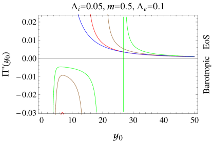
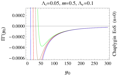
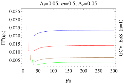
Figure 4: Stability of $d$-dimensional gravastar for barotropic EoS with exterior $d$-dimensional Schwarzschild-dS BH. It represents the initially unstable and then stable configuration of the developed structure.

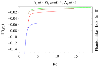
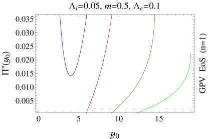
Figure 5: Stability of $d$-dimensional gravastar for Chaplygin and GCV EoS with exterior $d$-dimensional Schwarzschild-dS BH. Left plot shows unstable structure for Chaplygin model and right plot represents stable geometry for GCV EoS.

Figure 6: Stability of $d$-dimensional gravastar for phantomlike and GPV EoS with exterior $d$-dimensional Schwarzschild-dS BH. Left plot indicates unstable configuration for phantomlike EoS while right plot expresses stable structure for GPV EoS.

3.1.3 $d$-dimensional Reissner-Nordström BH

For $d$-dimensional RN BH, we have

$$\mathcal{Z}(y) = -\frac{2y^{2}\Lambda_{i}}{(d-2)(d-1)}+2my^{3-d}-Q^{2}y^{-2(d-3)},$$

$$\mathcal{W}(y) = -\frac{2y^{2}\Lambda_{i}}{(d-2)(d-1)}-2my^{3-d}+Q^{2}y^{-2(d-3)}+2.$$

We evaluate the respective expressions of the second derivative of effective potential with different matter distributions by using Eqs.(25), (29) and (32). The corresponding expressions of the second derivative of the effective potential for different matter distributions are analyzed graphically in Figures 7-9. The thin-shell gravastar represents an unstable structure for every choice of matter distribution with different values of $d$ while for higher values of $d$, the rate of the unstable structure decreases. For this choice of exterior geometry, the developed structure expresses unstable structure only.

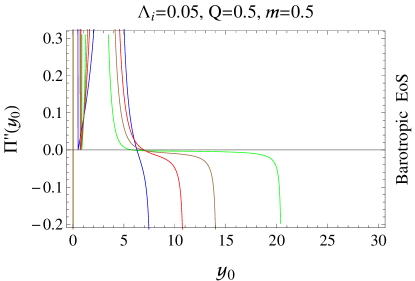
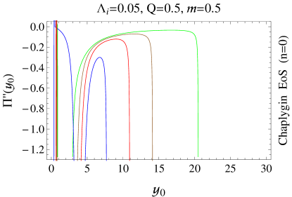
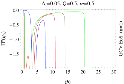
Figure 7: Unstable configuration of $d$-dimensional gravastar for barotropic EoS with exterior $d$-dimensional RN BH.

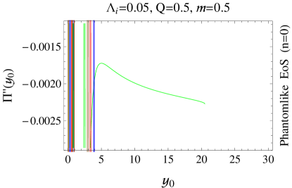
Figure 8: Unstable configuration of $d$-dimensional gravastar for Chaplygin and GCV EoS with exterior $d$-dimensional RN BH.

Figure 9: Unstable configuration of $d$-dimensional gravastar for phantomlike and GPV EoS with exterior $d$-dimensional RN BH.

3.1.4 $d$-dimensional Reissner-Nordström-dS BH

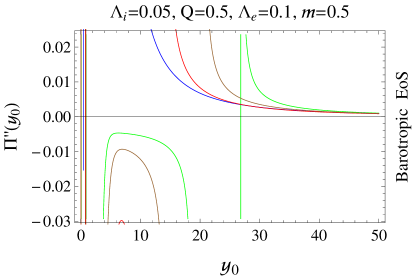
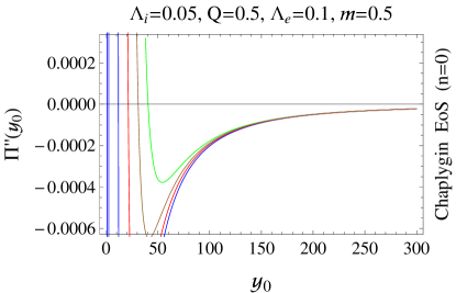
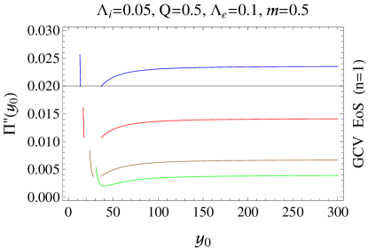
Figure 10: Stability of $d$-dimensional gravastar for barotropic EoS with exterior $d$-dimensional RN-dS BH. It is found that developed structure shows initially unstable then stable behavior for suitable physical parameters.

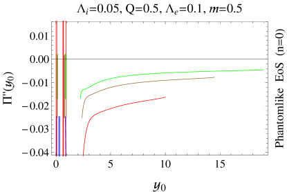
Figure 11: Stability of $d$-dimensional gravastar for Chaplygin and GCV EoS with exterior $d$-dimensional RN-dS BH. Left plot indicates unstable behavior for Chaplygin model and right plot shows stable configuration for GCV EoS.

Figure 12: Stability of $d$-dimensional gravastar for phantomlike and GPV EoS with exterior $d$-dimensional RN-dS BH. Left plot expresses unstable behavior for phantomlike EoS and right plot represents the stable geometry for GPV EoS.

The respective expressions of $\mathcal{Z}(y)$ and $\mathcal{W}(y)$ are given as

$$\mathcal{Z}(y) = \frac{2y^{2}\Lambda_{e}}{(d-2)(d-1)}-\frac{2y^{2}\Lambda_{i}}{(d-2)(d-1)}+2my^{3-d}-Q^{2}y^{-2(d-3)},$$

$$\mathcal{W}(y) = 2-\frac{2y^{2}\Lambda_{e}}{(d-2)(d-1)}-\frac{2y^{2}\Lambda_{i}}{(d-2)(d-1)}-2my^{3-d}+Q^{2}y^{-2(d-3)}.$$

The stable configurations are analyzed by using Eqs.(25), (29) and (32) as shown in Figures 10-12. We see that the developed structure indicates partially stable behavior for barotropic type fluid distribution (Figure 10) and unstable structure for Chaplygin as well as phantomlike EoS (left plots of Figures 11 and 12). For GCV and GPV EoS, thin-shell gravastars show stable configuration for every value of $d$ (right plots of Figures 11 and 12).

4 Conclusions

This paper studies stable configurations of gravastars through linearized radial perturbations for higher dimensions. We consider higher-dimensional BH spacetimes in the exterior of gravastars and explore their stability for three different types of matter distributions, i.e., barotropic, GCV, and GPV EoS. We have developed a geometrical structure of $d$-dimensional gravastars through the joining of inner $d$-dimensional dS and outer $d$-dimensional spherically symmetric BH spacetimes by using the cut and paste approach. We have considered Lanczos equations to obtain matter contents located at the hypersurface. The linearized radial perturbation is applied to the potential function of thin-shell to explore stable configurations.

Firstly, we have studied stable configurations of gravastar structure in the background of exterior $d$-dimensional Schwarzschild BH. We have found that the developed structure expresses unstable configurations for every type of matter distribution (Figures 1-3). For the exterior $d$-dimensional Schwarzschild-dS BH, we have obtained unstable structure for barotropic, Chaplygin, and phantomlike models while stable structure is found for GCV and GPV models for every suitable value of physical parameters (Figures 4-6).

For the $d$-dimensional RN manifold, the developed framework represents unstable configurations (Figures 7-9) while for $d$-dimensional RN-dS manifold, the structure indicates unstable behavior (for barotropic, Chaplygin, and phantomlike models) but stable configurations for GCV and GPV models (Figures 10-12). Hence, the $d$-dimensional Schwarzschild/RN-dS geometries lead to stable structure as compared to $d$-dimensional Schwarzschild/RN BHs. We conclude that the presence of cosmological constant in the exterior of gravastar geometry leads to stable structure for GCV and GPV type fluid distributions. It is worthwhile to mention here that stable configuration of higher-dimensional gravastar has similar behavior to four-dimensional gravastar.

References

• [1] P. Mazur, E. Mottola, Gravitational condensate stars: An alternative to black holes, arXiv: gr-qc/0109035.
• [2] P. Mazur, E. Mottola, Gravitational vacuum condensate stars, Proc. Nat. Acad. Sci. 101 (2004) 9545.
• [3] M. Visser, S. Kar, N. Dadhich, Traversable wormholes with arbitrarily small energy condition violations, Phys. Rev. Lett. 90 (2003) 201102.
• [4] M. Sharif, F. Javed, Collapse and expansion of scalar thin-shell for a class of black holes, Int. J. Mod. Phys. D 28 (2019) 1950046; Dynamical evolution of scalar field thin-shell for rotating regular black holes, Ann. Phys. 407 (2019) 198; Stability of Einstein-power-Maxwell (2+1)-dimensional wormholes, Chin. J. Phys. 61 (2019) 262; Dynamics of scalar shell for rotating and charged rotating BTZ black holes, Mod. Phys. Lett. A 35 (2019) 1950350.
• [5] M. Sharif, F. Javed, Stability of charged Kiselev thin-shell wormholes, Int. J. Mod. Phys. A 35 (2020) 2040015; Stability of charged rotating (2 + 1)-dimensional wormholes, Int. J. Mod. Phys. D 29 (2020) 2050007; Mechanical stability of a class of regular thin-shell wormholes, Mod. Phys. Lett. A 39 (2020) 2050309; Dynamics of thin-shell wormholes with rotational effects, Int. J. Mod. Phys. A 35 (2020) 2050030.
• [6] M. Visser, D.L. Wiltshire, Stable gravastars an alternative to black holes?, Class. Quantum Grav. 21 (2004) 1135.
• [7] D. Horvat, S. Ilijic, Gravastar energy conditions revisited, Class. Quantum Grav. 24 (2007) 5637.
• [8] B.M.N. Carter, Stable gravastars with generalized exteriors, Class. Quantum Grav. 22 (2005) 4551.
• [9] D. Horvat, S. Sasa Ilijic, A. Marunovic, Electrically charged gravastar configurations, Class. Quantum Grav. 26 (2009) 025003.
• [10] F. Rahaman, A.A. Usmani, S. Ray, S. Islam, The (2+1)-dimensional gravastars, Phys. Lett. B 707 (2012) 319; The (2+1)-dimensional charged gravastars, ibid. 717 (2012) 1.
• [11] C.F.C. Brandt, et al., Charged gravastar in a dark energy universe, J. Mod. Phys. 4 (2013) 869.
• [12] P. Rocha, et al., Bounded excursion stable gravastars and black holes, J. Cosmol. Astropart. Phys. 06 (2008) 25; R. Chan, M.F.A. da Silva, P. Rocha, A. Wang, Stable gravastars of anisotropic dark energy, J. Cosmol. Astropart. Phys. 03 (2009) 10.
• [13] R. Chan, M.F.A. da Silva, P. Rocha, How the cosmological constant affects gravastar formation, J. Cosmol. Astropart. Phys. 12 (2009) 17.
• [14] R. Chan, M.F.A. da Silva, How the charge can affect the formation of gravastars, J. Cosmol. Astropart. Phys. 07 (2010) 29.
• [15] F.S.N. Lobo, A.V.B. Arellano, Gravastars supported by nonlinear electrodynamics, Class. Quantum Grav. 24 (2007) 1069.
• [16] F.S.N. Lobo, R. Garattini, Linearized stability analysis of gravastars in noncommutative geometry, J. High Energy Phys. 1312 (2013) 065.
• [17] A. Γ–vgΓΌn, A. Banerjee, K. Jusufi, Charged thin-shell gravastars in noncommutative geometry, Eur. Phys. J. C 77 (2017) 566.
• [18] M. Sharif, F. Javed, Stability of gravastars with exterior regular black holes, Ann. Phys. 415 (2020) 168124; Stability of charged thin-shell gravastars with quintessence, Eur. Phys. J. C 81 (2021) 47.
• [19] A.A. Usmani, et al., Charged gravastars admitting conformal motion, Phys. Lett. B 701 (2011) 388.
• [20] P. Bhar, Higher dimensional charged gravastar admitting conformal motion, Astrophys. Space Sci. 354 (2014) 457.
• [21] Ghosh, S., Rahaman, F., Guha, B.K. and Ray, S., Charged gravastars in higher dimensions, Phys. Lett. B 767 (2017) 380; Gravastars with higher dimensional spacetimes, Ann. Phys. 394 (2018) 230.
• [22] G.A.S. Dias, J.P.S. Lemos, Thin-shell wormholes in $d$-dimensional general relativity: Solutions, properties, and stability, Phys. Rev. D 82 (2010) 084023.
• [23] E.F. Eiroa, C. Simeone, Aspects of spherical shells in a $d$-dimensional background, Int. J. Mod. Phys. D 21 (2012) 1250033.
• [24] A. Banerjee, K. Jusufi, S. Bahamonde, Stability of a $d$-dimensional thin-shell wormhole surrounded by quintessence, Gravit. Cosmol. 24 (2018) 1.
• [25] M. Sharif, F. Javed, Dynamics of the scalar shell in higher dimensions, Ann. Phys. 416 (2020) 168146; Stability and dynamics of regular thin-shell gravastars, J. Exp. Theor. Phys. 132 (2021) 381.
• [26] R.A. Konoplya, A. Zhidenko, Stability of multidimensional black holes: Complete numerical analysis, Nucl. Phys. B 777 (2007) 182; Stability of higher dimensional Reissner-NordstrΓΆm-anti-de Sitter black holes, Phys. Rev. D 78 (2008) 104017.
• [27] V. Varela, Note on linearized stability of Schwarzschild thin-shell wormholes with variable equations of state, Phys. Rev. D 92 (2015) 044002.
• [28] M. Sharif, F. Javed, On the stability of bardeen thin-shell wormholes, Gen. Relativ. Gravit. 48 (2016) 158; Linearized stability of Bardeen anti-de Sitter wormholes, Astrophys. Space. Sci. 364 (2019) 179. Stability of charged thin-shell and thin-shell wormholes: A comparison, Phys. Scr. 96 (2021) 055003.
• [29] E.F. Eiroa, C. Simeone, Stability of Chaplygin gas thin-shell wormholes, Phys. Rev. D 76 (2007) 024021.
• [30] P.K.F. Kuhfittig, The stability of thin-shell wormholes with a phantom-like equation of state, Acta Phys. Polon. B 41 (2010) 2017.