Deploying the Conditional Randomization Test
in High Multiplicity Problems

Abstract

This paper introduces the sequential CRT, which is a variable selection procedure that combines the conditional randomization test (CRT) and Selective SeqStep+. Valid $p\operatorname{-values}$ are constructed via the flexible CRT, which are then ordered and passed through the selective SeqStep+ filter to produce a list of discoveries. We develop theory guaranteeing control on the false discovery rate (FDR) even though the $p\operatorname{-values}$ are not independent. We show in simulations that our novel procedure indeed controls the FDR and are competitive with—and sometimes outperform—state-of-the-art alternatives in terms of power. Finally, we apply our methodology to a breast cancer dataset with the goal of identifying biomarkers associated with cancer stage.

1 Introduction

To quote from Benjamini and Hechtlinger [1],

Significance testing is an effort to address the selection of an interesting finding regarding a single parameter from the background noise. Modern science faces the problem of selection of promising findings from the noisy estimates of many.

This paper is about the latter. In contemporary studies, geneticists may have measured hundreds of thousands of genetic variants and wish to know which of these influence a trait [2; 3]. Scientists may be interested in discovering which demographic and clinical variables influence the susceptibility to Parkinson’s disease [4]. Economists study which variables from individual employment and wage histories affect future professional careers [5]. In all these examples and countless others, we have hundreds or even thousands of explanatory variables and are interested in determining which of these influence a response of interest. The problem is to select associations which are replicable, that is, without having too many false positives.

Formally, let $Y\in\mathbb{R}$ be the response we wish to study, and $X=(X_{1},X_{2},\ldots,X_{p})\in\mathbb{R}^{p}$ be the vector of explanatory variables. We call variable $j$ a null variable if $X_{j}$ is conditionally independent of $Y$ given the other $X$’s. This says that the $j$-th variable does not provide information about the response beyond what is already provided by all the other variables (roughly, if it is not in the Markov blanket of $Y$). Expressed differently, a variable is null if and only if the hypothesis

$$\mathcal{H}_{j}:X_{j}\mathchoice{\mathrel{\hbox to0.0pt{$\displaystyle\perp$\hss}\mkern 2.0mu{\displaystyle\perp}}}{\mathrel{\hbox to0.0pt{$\textstyle\perp$\hss}\mkern 2.0mu{\textstyle\perp}}}{\mathrel{\hbox to0.0pt{$\scriptstyle\perp$\hss}\mkern 2.0mu{\scriptstyle\perp}}}{\mathrel{\hbox to0.0pt{$\scriptscriptstyle\perp$\hss}\mkern 2.0mu{\scriptscriptstyle\perp}}}Y|X_{-j},$$ (1)

is true. (Throughout, $X_{-j}$ is a shorthand for all $p$ variables except the $j$th.) Likewise, a variable $j$ is nonnull if $\mathcal{H}_{j}$ is false. Let $\mathcal{H}_{0}\subset\left\{1,\dots,p\right\}$ be the subset of nulls. Suppose now we have $n$ independent samples assembled in a data matrix $\mathbf{X}\in\mathbb{R}^{n\times p}$ and a response vector $\mathbf{Y}\in\mathbb{R}^{n}$. The goal is to identify the nonnull variables with some form of type-I error control. Specifically, we consider in this paper the false discovery rate (FDR) [6], namely, the expected fraction of false positives defined as

$$\operatorname{FDR}=\mathbb{E}\left[\frac{|\hat{\mathcal{S}}\cap\mathcal{H}_{0}|}{|\hat{\mathcal{S}}|\vee 1}\right],.$$ (2)

where $\hat{\mathcal{S}}$ is the selected set of variables.

1.1 The conditional randomization test

Naturally, in order to identify the nonnull variables, one could test the hypotheses $\mathcal{H}_{j}$ in (1). Candès et al. [7] proposed to achieve this via the conditional randomization test (CRT). To run the CRT, we resample $\mathbf{X}_{j}$—the $j$th column of the matrix $\mathbf{X}$—conditional on the other variables, calculate the value of a test statistic, and compare it to the test statistic computed on the true $\mathbf{X}_{j}$. When the statistic computed on the true $\mathbf{X}_{j}$ has a high rank when compared with those obtained from imputed values, this is evidence against the null. Details of the CRT are given in Algorithm 1. There, the output p-value is valid in the sense that under the null, it is stochastically larger than a uniform variable.

Algorithm 1 Conditional Randomization Test (CRT)

0:  Data $(\mathbf{X},\mathbf{Y})$, test statistic $T(\cdot)$, number of randomizations $B$

  for $b\in\left\{1,\dots,B\right\}$ do

     Sample $\mathbf{X}_{j}^{(b)}$ from the distribution of $\mathbf{X}_{j}|\mathbf{X}_{-j}$, independently of $\mathbf{X}_{j}$ and $\mathbf{Y}$.

  end for

  The $p\operatorname{-value}$

$$p_{j}=\frac{1}{B+1}\left(1+\sum_{b=1}^{B}\mathbbm{1}{\left\{T(\mathbf{X}_{j},\mathbf{X}_{-j},\mathbf{Y})\leq T(\mathbf{X}_{j}^{(b)},\mathbf{X}_{-j},\mathbf{Y})\right\}}\right).$$

Informally, under the null hypothesis that the variable $X_{j}$ is independent of $Y$ conditional on $X_{-j}$, each one of the new samples $\mathbf{X}^{(b)}_{j}$ has the same distribution as $\mathbf{X}_{j}$, and they are all independent conditionally on $\mathbf{Y}$ and $\mathbf{X}_{-j}$. As a consequence, each $T(\mathbf{X}^{(b)}_{j},\mathbf{X}_{-j},\mathbf{Y})$ has the same distribution as $T(\mathbf{X}_{j},\mathbf{X}_{-j},\mathbf{Y})$. Thus the rank of $T(\mathbf{X}_{j},\mathbf{X}_{-j},\mathbf{Y})$ among $\left\{T(\mathbf{X}^{(b)}_{j},\mathbf{X}_{-j},\mathbf{Y})\right\}$ will be uniform in $\left\{1,\dots,B\right\}$ assuming we break ties at random. Formally, we have:

Theorem 1 (Candès et al. [7]).

If $X_{j}\mathchoice{\mathrel{\hbox to0.0pt{$\displaystyle\perp$\hss}\mkern 2.0mu{\displaystyle\perp}}}{\mathrel{\hbox to0.0pt{$\textstyle\perp$\hss}\mkern 2.0mu{\textstyle\perp}}}{\mathrel{\hbox to0.0pt{$\scriptstyle\perp$\hss}\mkern 2.0mu{\scriptstyle\perp}}}{\mathrel{\hbox to0.0pt{$\scriptscriptstyle\perp$\hss}\mkern 2.0mu{\scriptscriptstyle\perp}}}Y|X_{-j}$, then the $p\operatorname{-values}$ from Algorithm 1 satisfy $\mathbb{P}\left[p_{j}\leq\alpha\right]\leq\alpha$, for any $\alpha\in[0,1]$. This holds regardless of the test statistic $T(\cdot)$.

The validity of the procedure does not rely on any assumptions on the distribution of $Y|X$, parametric or not. Yet it requires knowledge of the distribution of the covariates $X$. This is known as the Model-X framework, and is an appropriate assumption in many important applications, including genetic and economics studies, where either knowledge about the exact covariate distribution or a large amount of unsupervised data of covariates is available [8; 9; 10; 11; 12]. Rapid progress has been made on methodological advances in this framework [7; 13; 2; 14; 15; 16; 17] and in applications to genetic studies [2; 3; 18].

1.2 Selective SeqStep+

We still need a selection procedure that transforms the CRT $p\operatorname{-values}$ into a selected set with FDR control guarantees. A natural choice of variable selection procedure is the Benjamini-Hochberg procedure (BHq) [6]. If we were to apply BHq, we would need to compare the $p\operatorname{-values}$ with critical thresholds of the form $\alpha_{i}=iq/p$, where $q$ is the nominal FDR level. When $p$ is large, $q$ is $0.1$, and $i=1,2,\dots$, this requires $p\operatorname{-values}$ on an extremely fine scale. The $p\operatorname{-values}$ defined in Algorithm 1, however, can only take values in $\{1/(B+1),2/(B+2),\dots,1\}$, thus a huge number of randomizations in CRT is required. This makes the combination of CRT and BHq computationally expensive or even infeasible. This is the motivation for this paper: can we find a selection procedure that does not require any of the $p\operatorname{-values}$ to be very small and works well with discrete $p\operatorname{-values}$?

Algorithm 2 Selective SeqStep+

0:  A sequence of $p\operatorname{-values}$ $p_{1},\dots p_{p}$

  Let

$$\hat{k}=\max\left\{k\in\left\{1,\dots,p\right\}:\frac{1+\#\left\{j\leq k:p_{j}>c\right\}}{\#\left\{j\leq k:p_{j}\leq c\right\}\vee 1}\leq\frac{1-c}{c}\cdot q\right\}.$$ (3)

  Selected set of nonnulls $\hat{\mathcal{S}}=\left\{j\leq\hat{k}:p_{j}\leq c\right\}$. If the set in $\eqref{eqn:seqstep}$ is empty, $\hat{\mathcal{S}}$ is the empty set as well.

To this end, we consider SeqStep+, a sequential testing procedure first introduced by Barber and Candès [19]. We consider a specific version, namely, Selective SeqStep+, which takes a sequence of $p\operatorname{-values}$ $p_{1},\dots p_{p}$ as input, and outputs a selected set $\hat{\mathcal{S}}$. The procedure starts by finding an integer $\hat{k}$ such that among the $p\operatorname{-values}$ $\left\{p_{1},\dots,p_{\hat{k}}\right\}$, few are greater than a user-specified threshold $c$. In details, $\hat{k}$ is the largest $k$ in $\left\{1,\dots p\right\}$ such that the ratio between $1+\#\left\{j\leq k:p_{j}>c\right\}$ and $\#\left\{j\leq k:p_{j}\leq c\right\}\vee 1$ is no greater than $(1-c)q/c$. The procedure then selects all $j$’s, such that $j\leq\hat{k}$ and $p_{j}\leq c$. We include details of the procedure in Algorithm 2.

To understand why the procedure works, assume that the null $p\operatorname{-values}$ are $\text{i.i.d.}\operatorname{Unif}[0,1]$. Then, the ratio of $\#\left\{\text{null }j\leq\hat{k}:p_{j}\leq c\right\}$ to $\#\left\{\text{null }j\leq\hat{k}:p_{j}>c\right\}$ is roughly $c/(1-c)$. Hence

$$\operatorname{FDP} =\frac{\#\left\{\text{null }j\leq\hat{k}:p_{j}\leq c\right\}}{\#\left\{j\leq\hat{k}:p_{j}\leq c\right\}\vee 1}\approx\frac{c}{1-c}\cdot\frac{\#\left\{\text{null }j\leq\hat{k}:p_{j}>c\right\}}{\#\left\{j\leq\hat{k}:p_{j}\leq c\right\}\vee 1}$$

$$\leq\frac{c}{1-c}\cdot\frac{\#\left\{j\leq\hat{k}:p_{j}>c\right\}}{\#\left\{j\leq\hat{k}:p_{j}\leq c\right\}\vee 1}\leq\frac{c}{1-c}\cdot\frac{1-c}{c}q=q.$$

Formally, we have the following result.

Theorem 2 (Barber and Candès [19]).

Assume that the ordering of the $p\operatorname{-values}$ is fixed. If all null $p\operatorname{-values}$ are independent with $p_{j}\geq\operatorname{Unif}[0,1]$, and are independent from the nonnulls, then Selective SeqStep+ controls the FDR at level $q$.

A close look at (3) shows that the only information Selective SeqStep+ uses from the $p\operatorname{-values}$ is whether or not $p_{j}\leq c$. This means that unlike BHq, Selective SeqStep+ does not require some of the $p\operatorname{-values}$ to be very small to make rejections, and hence would require a much smaller number of randomizations $B$. Selective SeqStep+ would, therefore, be computationally far less intensive.

1.3 Challenges and our contribution

In this paper, we study variable selection procedures with the conditional randomization test and Selective SeqStep+. There are three challenges and we address them all.

The first challenge is in the dependency of the $p\operatorname{-values}$. The $p\operatorname{-values}$ from CRT are not independent in general, hence Theorem 2 does not apply. In response, we will develop theory in Section 2 showing how we can make SeqStep+ valid under dependence. In particular, we will show examples of approximate FDR control when the $p\operatorname{-values}$ are weakly dependent or when they are exchangeable in distribution.

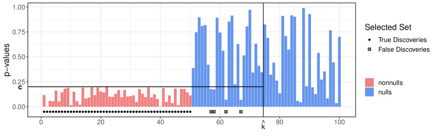
(a) A good ordering

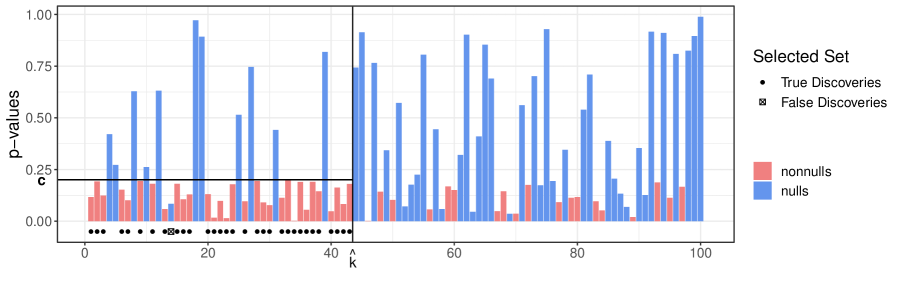
(b) A bad ordering

Figure 1: An illustration of the ordering of the $p\operatorname{-values}$ in Selective SeqStep+. The null $p\operatorname{-values}$ are sampled from $\operatorname{Unif}[0,1]$ and the nonnull $p\operatorname{-values}$ from $\operatorname{Unif}[0,0.2]$. We take $c=0.2$ and $q=0.1$. The $p\operatorname{-values}$ are the same in the two plots, but they are ordered in two different ways. In (a), the nonnulls appear early in the sequence. In (b), the order of the $p\operatorname{-values}$ is random. In terms of power, Selective SeqStep+ discovers all the nonnulls in (a) but only a subset of them in (b).

The second challenge concerns the ordering of the $p\operatorname{-values}$. Unlike the Benjamini-Hochberg procedure, which takes as input the $p\operatorname{-values}$ only, Selective SeqStep+ essentially requires two inputs: the $p\operatorname{-values}$ and an ordering of the $p\operatorname{-values}$. In other words, if we change the order of the input $p\operatorname{-values}$, we could end up selecting a very different set of variables. To illustrate this, consider the example in Figure 1, which fixes the $p\operatorname{-values}$ and compare two different orderings. The “good” ordering has the nonnulls appear early in the sequence and the “bad” ordering randomly permutes the $p\operatorname{-values}$. With the good ordering, the output set contains all the nonnulls; but with the bad ordering, only a fraction of the nonnulls is discovered. When the nonnull $p\operatorname{-values}$ appear early in the sequence, the proportion of $p\operatorname{-values}$ greater than $c$ will be smaller, thus the quantity $\frac{1+\#\left\{j\leq k:p_{j}>c\right\}}{\#\left\{j\leq k:p_{j}\leq c\right\}\vee 1}$ in (3) will tend to be smaller. Therefore a larger $\hat{k}$ will be obtained and hence the power of the procedure will be higher. In general, to make the variable selection procedure more powerful, it is important to look for an informative ordering that places nonnulls early in the sequence.

Another requirement for the ordering is that it needs to be independent of the $p\operatorname{-values}$. FDR is in general not controlled when the $p\operatorname{-values}$ and the ordering are dependent. As a simple example, assume a researcher obtains independent $p\operatorname{-values}$ and naively orders them by magnitude. Then the input sequence of $p\operatorname{-values}$ into Selective SeqStep+ would be an ordered sequence $p_{(1)}\leq p_{(2)}\dots\leq p_{(p)}$. In this case, the null $p\operatorname{-values}$ that appear early in the sequence will tend to be smaller and hence no longer uniform. In the case of the global null (all hypotheses are null) with independent $p\operatorname{-values}$, we would expect to make around $cp$ false discoveries. This is because there are approximately $cp$ $p\operatorname{-values}$ that are smaller than or equal to $c$, and they all appear early in the sequence, hence for $k=(c+(1-c)q)p$,

$$\frac{1+\#\left\{j\leq k:p_{j}>c\right\}}{\#\left\{j\leq k:p_{j}\leq c\right\}\vee 1}\approx\frac{(c+(1-c)q)p-cp}{cp}=\frac{(1-c)q}{c}.$$

In Section 3, we will present two methods to obtain the ordering: the split version and the symmetric statistic version. The former splits the data into two parts, obtaining $p\operatorname{-values}$ from one fold, and the ordering from the other. This makes the ordering and the $p\operatorname{-values}$ stochastically independent. No data-splitting is required for the symmetric statistic version; we obtain both the $p\operatorname{-values}$ and the ordering from the whole dataset. To obtain the ordering, we compute a statistic $z_{j}$ for each variable $j$, and sort the $z_{j}$’s. The statistic $z_{j}$ is obtained in such a way that $z_{j}$ is marginally independent of the $p\operatorname{-value}$ $p_{j}$. In theory, this notion of independence is not sufficient for FDR control; we however tested this method in many different empirical settings and always controlled the $\operatorname{FDR}$. In terms of power, the symmetric statistic version is more powerful than the split version. Thus in practice, we would recommend the symmetric statistic version.

The third challenge is computational in nature. Recall that with the CRT (Algorithm 1), we need to compute the test statistic $T_{j}^{(b)}$ for each $j$ and each $b$. Each statistic $T_{j}^{(b)}$ is obtained by sampling $\mathbf{X}_{j}^{(b)}$ and running a machine learning algorithm with $\mathbf{Y}$ as a response and $\mathbf{X}_{j}^{(b)},\mathbf{X}_{-j}$ as predictors. It is computationally expensive to run the machine learning algorithm $B$ times to get a single $p\operatorname{-value}$. In Section 4, we will present a faster way of obtaining the test statistics and, hence, the $p\operatorname{-values}$.

2 Selective SeqStep+ under dependence

2.1 Almost independent $p$-values

When employing SeqStep+, it is natural to ask whether the FDR is still controlled when the $p\operatorname{-values}$ are “close” to being independent. This section derives an bound upper bound on the FDR, which depends on the value of $\max_{j\in\mathcal{H}_{0}}\mathbb{P}[p_{j}\leq c\mid\mathbbm{1}\left\{p_{-j}\leq c\right\}]$, the maximum of the probability that $p_{j}$ is at most $c$ conditional on the boolean sequence of whether other $p\operatorname{-values}$ are smaller than or equal to $c$. Under independence of the $p\operatorname{-values}$, it holds that $\max_{j\in\mathcal{H}_{0}}\mathbb{P}\left[p_{j}\leq c\mid\mathbbm{1}\left\{p_{-j}\leq c\right\}\right]\leq c$ since marginally, $\mathbb{P}\left[p_{j}\leq c\right]\leq c$ for $j\in\mathcal{H}_{0}$. Our first result states that if $\max_{j\in\mathcal{H}_{0}}\mathbb{P}\left[p_{j}\leq c\mid\mathbbm{1}\left\{p_{-j}\leq c\right\}\right]$ is close to $c$ with high probability, then the FDR inflation cannot be large.

Theorem 3 (Almost independent $p$-values).

Suppose the ordering of the $p\operatorname{-values}$ is fixed. Set $a_{j}=\mathbb{P}\left[p_{j}\leq c\mid\mathbbm{1}\left\{p_{-j}\leq c\right\}\right]$ and assume the $p\operatorname{-values}$ satisfy $\mathbb{P}\left[\max_{j\in\mathcal{H}_{0}}a_{j}\leq c+\delta\right]\geq 1-\epsilon$. Then the output from Algorithm 2 obeys

$$\operatorname{FDR}\leq q\frac{c+\delta}{c}\frac{1-c}{1-c-\delta}+\epsilon.$$ (4)

As an illustration, we describe two examples where the FDR bound can be computed numerically. Consider data $(\mathbf{X},\mathbf{Y})$, where each row of $\mathbf{X}$ is generated independently from a multivariate Gaussian distribution with block diagonal covariance; that is, $X_{j}$ is only dependent on nearby variables. Recalling that the $p\operatorname{-values}$ are obtained from Algorithm 1, the first example takes the marginal test statistic to be $T(\mathbf{X}_{j},\mathbf{X}_{-j},\mathbf{Y})=\left|\operatorname{Corr}\left[\mathbf{X}_{j},\mathbf{Y}\right]\right|$, whereas in the second example, we regress $\mathbf{Y}$ on $\mathbf{X}_{j}$ and $\mathbf{X}_{N(j)}$, and take the test statistic $T(\mathbf{X}_{j},\mathbf{X}_{-j},\mathbf{Y})$ to be the absolute value of the fitted coefficient of $\mathbf{X}_{j}$. Here, the elements of $N(j)$ are the “neighbors” of $j$, i.e. the indices in the same block as $j$. Additional details of the simulation settings are included in Appendix A.6.

Before proceeding with the computation, we note that if $a_{j}$ were defined conditional on additional information, e.g. $a_{j}=\mathbb{P}\left[p_{j}\leq c\mid\mathbf{Y},\mathbbm{1}\left\{p_{-j}\leq c\right\}\right]$, then Theorem 3 would still hold. The specific block diagonal structure of the covariance of $X$ implies that $X_{i}$ and $X_{j}$ are independent conditionally on $Y$ if $i$ and $j$ are not in the same block. Thus, $a_{j}=\mathbb{P}\left[p_{j}\leq c\mid\mathbf{Y},\mathbbm{1}\left\{p_{-j}\leq c\right\}\right]=\mathbb{P}\left[p_{j}\leq c\mid\mathbf{Y},\mathbbm{1}\left\{p_{N(j)}\leq c\right\}\right]$. For a block of size $K$, the variable $\mathbbm{1}\left\{p_{N(j)}\leq c\right\}$ can take at most $2^{K}$ distinct values. In practice, the conditional probability $\mathbb{P}\left[p_{j}\leq c\mid\mathbf{Y},\mathbbm{1}\left\{p_{N(j)}\leq c\right\}\right]$ can therefore be estimated using sample proportions. One can fix $\mathbf{Y}$, sample $\mathbf{X}$ from the distribution of $X\mid Y$, compute the corresponding $p\operatorname{-values}$, and compute the frequency of the event $\left\{p_{j}\leq c\right\}$ conditional on the value of $\mathbbm{1}\left\{p_{N(j)}\leq c\right\}$. This is the reason why the block diagonal structure of the covariance is used here; this structure makes computations tractable since we are dealing with $2^{K}$ rather than $2^{p-1}$ possible configurations.

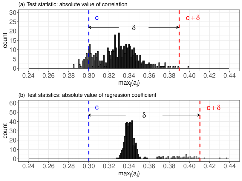
Figure 2: Histogram of $\max_{j\in\mathcal{H}_{0}}a_{j}$ from 500 samples. In (a), the test statistic of CRT is taken to be the absolute value of the correlation. In (b), the test statistic of CRT is taken to be the absolute value of the regression coefficient. We plot the threshold $c$ (blue dashed line). To apply the bound from Theorem 3, one possible choice of $\delta$ is shown as the distance between the red and blue lines.

In Figure 2, we plot the histogram of $\max_{j\in\mathcal{H}_{0}}a_{j}=\max_{j\in\mathcal{H}_{0}}\mathbb{P}\left[p_{j}\leq c\mid\mathbf{Y},\mathbbm{1}\left\{p_{N(j)}\leq c\right\}\right]$ from 500 samples and show a possible choice of $\delta$ and $\epsilon$. Here, the FDR threshold $q$ is set to be 0.1 and $c$ is chosen to be $0.3$. In the example where the test statistic is the absolute value of correlation between $\mathbf{X}$ and $\mathbf{Y}$, we can take $\delta=0.0893$ and $\epsilon=0.002$. The FDR bound in (4) is thus $q\frac{c+\delta}{c}\frac{1-c}{1-c-\delta}+\epsilon=0.1508$. In the other example where the test statistic is the absolute value of the fitted regression coefficient, we can take $\delta=0.11$ and $\epsilon=0.006$. The FDR bound in (4) is thus $q\frac{c+\delta}{c}\frac{1-c}{1-c-\delta}+\epsilon=0.1682$.

2.2 Under exchangeability

In this section, we study whether additional structure on the $p\operatorname{-values}$ can be helpful in obtaining sharper FDR bounds. To this end, consider the assumption of exchangeability. We say that the random variables $A_{1},A_{2},\dots,A_{m}$ are exchangeable conditional on a random variable $B$ if $(A_{1},\dots,A_{m})\mid B\stackrel{{\scriptstyle d}}{{=}}(A_{\pi(1)},\ldots,A_{\pi(m)})\mid B$ for any permutation $\pi$. With this, this section makes use of the following assumption:

Assumption 1.

The null $p\operatorname{-values}$ are exchangeable conditional on the nonnull $p\operatorname{-values}$.

To understand Assumption 1, we study examples where it holds. Consider $p\operatorname{-values}$ obtained from the CRT. A sufficient set of conditions is that the variables $X_{j}$’s are exchangeable and that the test statistic $T(\cdot)$ in the CRT (Algorithm 1) is symmetric in $\mathbf{X}_{-j}$. As a concrete example, imagine $X$ follows a $\mathcal{N}(\mathbf{\mu},\Sigma)$ distribution, where all entries in $\mu$ are the same and all off-diagonal terms in $\Sigma$ are the same. Then if $T(\mathbf{X}_{j},\mathbf{X}_{-j},\mathbf{Y})$ is obtained by running a lasso regression of $\mathbf{Y}$ on $\mathbf{X}$ and taking the regression coefficient of $j$, then the null $p\operatorname{-values}$ are exchangeable conditional on the nonnulls.

Under the assumption of exchangeability, we can show that FDR inflation will not be large. In particular, if the $p\operatorname{-values}$ are weakly correlated with each other, we get a sharper upper bound.

Theorem 4 (Under exchangeability).

Suppose the ordering of the $p\operatorname{-values}$ is fixed and that the nulls are marginally stochastically larger than uniform. Under Assumption 1, Algorithm 2 gives

$$\operatorname{FDR}\leq q+c(1-q).$$ (5)

If, in addition, the $p\operatorname{-values}$ satisfy $\operatorname{Corr}\left[\mathbbm{1}\left\{p_{i}\leq c\right\},\mathbbm{1}\left\{p_{j}\leq c\right\}\right]\leq\rho$ for any nulls $i\neq j$, then

$$\operatorname{FDR}\leq q+\varepsilon(c,q,\rho),$$ (6)

where

$$\varepsilon(c,q,\rho)=\left(\frac{\delta}{1+\beta\delta}\left[\frac{c}{1-c}-\frac{c-c\delta}{1-(c-c\delta)}q\right]\right)\wedge c(1-q),\quad\beta=\frac{c+(1-c)q}{(1-c)(1-q)},\quad\delta=\rho\frac{c(1-q)+q}{c(1-q)}.$$

The two bounds (5) and (6) are sharp asymptotically. For illustration, the bound (6) is plotted in Figure 3.

Proof.

We will show the asymptotic sharpness of (5) here. Specifically, we will show an example where the $\operatorname{FDR}$ converges to $q+c(1-q)$ as $p\to\infty$. We include a proof of the two upper bounds and the asymptotic sharpness of (6) in Appendix B.1.

Assume we are under the global null, i.e., all variables are nulls. Set $m_{0}=1+\lceil\frac{cp}{q+c(1-q)}\rceil$ and consider null $p\operatorname{-values}$ sampled as follows:

1. With probability $cp/m_{0}$, pick $m_{0}$ indices uniformly at random from $\left\{1,\dots,p\right\}$, and sample the corresponding $p\operatorname{-values}$ as $\text{i.i.d.}\operatorname{Unif}[0,c]$; sample the other $p\operatorname{-values}$ independently from $\operatorname{Unif}[c,1]$.

2. With probability $1-cp/m_{0}$, sample all $p\operatorname{-values}$ as $\text{i.i.d.}\operatorname{Unif}[c,1]$.

One can easily verify that each $p\operatorname{-value}$ marginally follows a $\operatorname{Unif}[0,1]$ distribution. On the first event, we always reject all the variables because

$$\frac{1+\#\left\{j\leq p:p_{j}>c\right\}}{\#\left\{j\leq p:p_{j}\leq c\right\}\vee 1}=\frac{1+p-m_{0}}{m_{0}}\leq\frac{1+p-m_{0}}{m_{0}-1}\leq\frac{1-c}{c}\cdot q.$$

Thus $\operatorname{FDP}=1$. On the second event, we reject none of the variables, thus $\operatorname{FDP}=0$. Combining the two cases, we get $\operatorname{FDR}=cp/m_{0}\to q+c(1-q)$ as $p\to\infty$. ∎

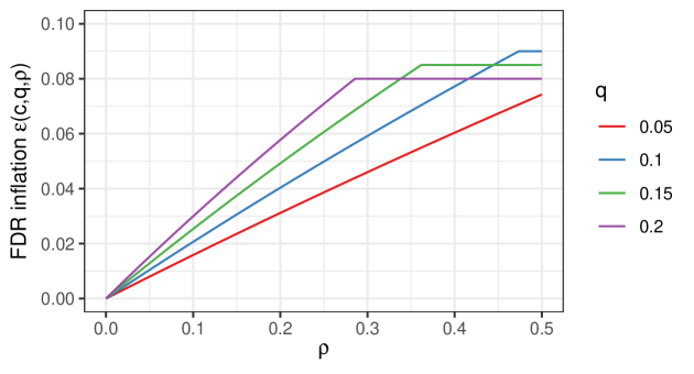
Figure 3: The bound on FDR inflation $\varepsilon(c,q,\rho)$. Here we set $c=0.1$, vary $\rho$ from 0 to 0.5, and vary the FDR threshold $q$ from $0.05$ to $0.2$.

Compared to the FDR bound in Theorem 3, Theorem 4 is neither weaker nor stronger. Theorem 4 holds when the null $p\operatorname{-values}$ are exchangeable, whereas Theorem 3 holds when the $p\operatorname{-values}$ are close to being independent. When the $p\operatorname{-values}$ are exchangeable and highly correlated, for example in the most extreme case where all the $p\operatorname{-values}$ are the same, then (5) in Theorem 4 gives that $\operatorname{FDR}\leq q+c(1-q)$, whereas (4) in Theorem 3 would not be informative at all. In a different setting where the $p\operatorname{-values}$ are independent but follow different distributions, Theorem 3 can be used to show that $\operatorname{FDR}\leq q$, whereas Theorem 4 cannot be applied.

2.3 Beyond exchangeability or almost independence of the $p$-values

In general, when the $p\operatorname{-values}$ have an arbitrary dependence structure, we can bound the FDR with a logarithmic inflation; the sharpness of the bound below is an open question.

Theorem 5 (Arbitrary dependence).

Suppose the ordering of the $p\operatorname{-values}$ is fixed and that the nulls are marginally stochastically larger than uniform. If $(1-c)q<c$, then Algorithm 2 yields

$$\operatorname{FDR}\leq(q+c(1-q))\sum_{j\in\mathcal{H}_{0}}\frac{1}{j+1}\leq(q+c(1-q))\log p.$$ (7)

When we have a good ordering of the $p\operatorname{-values}$, i.e., when the null $p\operatorname{-values}$ tend to have larger indices, then the right-hand side $(q+c(1-q))\sum_{j\in\mathcal{H}_{0}}\frac{1}{j+1}$ is smaller. Comparing to the case with exchangeability, we observe a potential logarithmic inflation on the FDR. A similar phenomenon has been observed for the BHq procedure, where an arbitrary dependence among the $p\operatorname{-values}$ also brings a possible logarithmic inflation [20].

3 Methods to order hypotheses

When performing variable selection with CRT and Selective SeqStep+, it is important to have a good ordering of the hypotheses/CRT $p\operatorname{-values}$. A naive way of obtaining the ordering is as follows: apply any machine learning algorithm to $(\mathbf{X},\mathbf{Y})$, compute a statistic $z_{j}$ providing evidence against the hypothesis that $j$ is null, sort the CRT $p\operatorname{-values}$ by decreasing order of the $z_{j}$’s, and apply Selective SeqStep+. As argued in Section 1.3, despite the intuitive structure of this procedure, the dependence between the $p\operatorname{-values}$ and the ordering will, in general, imply a loss of FDR control.

3.1 Splitting

Procedure 3 The Sequential CRT (Split version)

0:  Data $\mathcal{D}=(\mathbf{X},\mathbf{Y})$, number of randomizations $B$, test statistic $T(\cdot)$, score function $Z$, $\operatorname{FDR}$ threshold $q$, SeqStep threshold $c$.

1.   Split the data into two folds $\mathcal{D}_{\operatorname{pval}}=(\mathbf{X}^{\operatorname{pval}},\mathbf{Y}^{\operatorname{pval}})$ and $\mathcal{D}_{\operatorname{ordering}}=(\mathbf{X}^{\operatorname{ordering}},\mathbf{Y}^{\operatorname{ordering}})$.
2.   Obtain $p\operatorname{-values}$ $p_{1}\dots,p_{p}$ on $\mathcal{D}_{\operatorname{pval}}$ from CRT (Algorithm 1).
3.   Compute statistics $z_{j}=Z\left(\mathbf{X}_{j}^{\operatorname{ordering}},\mathbf{X}_{-j}^{\operatorname{ordering}},\mathbf{Y}^{\operatorname{ordering}}\right)$ on $\mathcal{D}_{\operatorname{ordering}}$ for each $j\in\left\{1,\dots p\right\}$, and obtain ordering $\pi$ by sorting the statistics: $z_{\pi(1)}\geq z_{\pi(2)}\dots\geq z_{\pi(p)}$.
4.   Apply Selective SeqStep+ (Algorithm 2) to $p_{\pi(1)},p_{\pi(2)},\dots,p_{\pi(p)}$.

0:  Discoveries from Selective SeqStep+.

The split version of the sequential CRT (Procedure 3) makes the $p\operatorname{-values}$ and ordering independent through data splitting: the data is split into two folds; the $p\operatorname{-values}$ are obtained from the CRT on the first fold; and the ordering is obtained on the second fold. Independence ensures that Theorem 3 holds for this procedure. The downside is that this suffers from a power loss as is the case for many other data splitting procedures. This motivates us to look for procedures that use the full data to obtain both the $p\operatorname{-values}$ and the ordering.

3.2 Symmetric statistics

As seen in Section 1.3, the correlation between the null $p\operatorname{-value}$ $p_{j}$ and the statistic $z_{j}$, which is sorted to obtain the ordering, largely accounts for the FDR inflation. It is thus natural to seek procedures that make $p_{j}$ and $z_{j}$ independent for nulls. To this end, recall that the $p\operatorname{-value}$ $p_{j}$ is defined as

$$p_{j}=\frac{1}{B+1}\left(1+\sum_{b=1}^{B}\mathbbm{1}\left\{T(\mathbf{X}_{j},\mathbf{X}_{-j},\mathbf{Y})\geq T(\mathbf{X}_{j}^{(b)},\mathbf{X}_{-j},\mathbf{Y})\right\}\right).$$

We propose a method with $p_{j}$ as above and each $z_{j}$ constructed as follows: consider a function $Z$ that is symmetric in its first $B+1$ arguments, and define

$$z_{j}=Z\left(\mathbf{X}_{j},\mathbf{X}_{j}^{(1)},\dots,\mathbf{X}_{j}^{(B)},\mathbf{X}_{-j},\mathbf{Y}\right).$$

This definition leads to Procedure 4.

Procedure 4 The Sequential CRT (Symmetric statistic version)

0:  Data $\mathcal{D}=(\mathbf{X},\mathbf{Y})$, number of randomizations $B$, test statistic $T(\cdot)$, score function $Z(\cdot)$ (symmetric in its first $B+1$ arguments), $\operatorname{FDR}$ threshold $q$, SeqStep threshold $c$.

1.   Obtain $p\operatorname{-values}$ $p_{1}\dots,p_{p}$ on $\mathcal{D}$ from CRT (Algorithm 1).
2.   Compute statistics: $z_{j}=Z\left(\mathbf{X}_{j},\mathbf{X}_{j}^{(1)},\dots,\mathbf{X}_{j}^{(B)},\mathbf{X}_{-j},\mathbf{Y}\right)$ for each $j\in\left\{1,\dots p\right\}$, and obtain an ordering $\pi$ by sorting the statistics: $z_{\pi(1)}\geq z_{\pi(2)}\dots\geq z_{\pi(p)}$.
3.   Apply Selective SeqStep+ (Algorithm 2) to $p_{\pi(1)},p_{\pi(2)},\dots,p_{\pi(p)}$.

0:  Discoveries from Selective SeqStep+.

Intuitively, the $p\operatorname{-value}$ $p_{j}$ is capturing the relative rank of $\mathbf{X}_{j}$ among $\left\{\mathbf{X}_{j}^{(1)},\dots,\mathbf{X}_{j}^{(B)}\right\}$, yet, $z_{j}$ is symmetric in $\left\{\mathbf{X}_{j},\mathbf{X}_{j}^{(1)},\dots,\mathbf{X}_{j}^{(B)}\right\}$. The symmetry allows us to permute elements in $\Big{\{}\mathbf{X}_{j},\mathbf{X}_{j}^{(1)},\dots,$ $\mathbf{X}_{j}^{(B)}\Big{\}}$ while keeping $z_{j}$ fixed. This means that $z_{j}$ is not providing information regarding the relative rank of $\mathbf{X}_{j}$ among $\left\{\mathbf{X}_{j}^{(1)},\dots,\mathbf{X}_{j}^{(B)}\right\}$ and is hence independent of $p_{j}$. Put formally:

Proposition 1.

The $p\operatorname{-value}$ $p_{j}$ and the statistic $z_{j}$ defined in Procedure 4 obey $p_{j}\mathchoice{\mathrel{\hbox to0.0pt{$\displaystyle\perp$\hss}\mkern 2.0mu{\displaystyle\perp}}}{\mathrel{\hbox to0.0pt{$\textstyle\perp$\hss}\mkern 2.0mu{\textstyle\perp}}}{\mathrel{\hbox to0.0pt{$\scriptstyle\perp$\hss}\mkern 2.0mu{\scriptstyle\perp}}}{\mathrel{\hbox to0.0pt{$\scriptscriptstyle\perp$\hss}\mkern 2.0mu{\scriptscriptstyle\perp}}}z_{j}$ for any null $j$. In addition, $p_{j}\mathchoice{\mathrel{\hbox to0.0pt{$\displaystyle\perp$\hss}\mkern 2.0mu{\displaystyle\perp}}}{\mathrel{\hbox to0.0pt{$\textstyle\perp$\hss}\mkern 2.0mu{\textstyle\perp}}}{\mathrel{\hbox to0.0pt{$\scriptstyle\perp$\hss}\mkern 2.0mu{\scriptstyle\perp}}}{\mathrel{\hbox to0.0pt{$\scriptscriptstyle\perp$\hss}\mkern 2.0mu{\scriptscriptstyle\perp}}}z_{j}|\mathbf{X}_{-j},\mathbf{Y}$, for any null $j$.

This result is a special case of Proposition 2 that will be presented later.

Note that Proposition 1 is not sufficient to guarantee FDR control. Even though $p_{j}$ is independent of $z_{j}$, $p_{j}$ could, in principle, still have a complicated relationship with $z_{-j}$. This makes the $p\operatorname{-values}$ not entirely independent of the ordering. This however does not appear to lead to FDR inflation in practice. We indeed observe FDR control in various simulation studies in Section 5.

The statistic $z_{j}$ can be computed using complicated machine learning methods. For example, one can run a gradient boosting algorithm with regression trees as base learners, $\mathbf{Y}$ as a response, and $\mathbf{X}_{j},\mathbf{X}_{j}^{(1)},\dots,\mathbf{X}_{j}^{(B)},\mathbf{X}_{-j}$ as predictors, obtain feature importance statistics of $\mathbf{X}_{j},\mathbf{X}_{j}^{(1)},\dots,\mathbf{X}_{j}^{(B)}$, and take $z_{j}$ to be the maximum of the statistics. One can easily verify that with this specific construction, $z_{j}$ is symmetric in $\left(\mathbf{X}_{j},\mathbf{X}_{j}^{(1)},\dots,\mathbf{X}_{j}^{(B)}\right)$.

4 Towards faster computation: one-shot CRT

In the original CRT (Algorithm 1), to compute each $p\operatorname{-value}$ $p_{j}$ one runs a machine learning algorithm $B$ times to obtain the test statistics $T_{j}^{(b)}$ for $b\in\left\{1,\dots,B\right\}$. This quickly gets computationally expensive when the machine learning algorithm is run on a large dataset. To save computation time, another way of computing the statistics is to run the machine learning algorithm once, with $\mathbf{Y}$ as a response and $\mathbf{X}_{j},\mathbf{X}_{j}^{(1)},\dots,\mathbf{X}_{j}^{(B)},\mathbf{X}_{-j}$ as the predictors. Formally, we consider a procedure $T$ that takes $\left(\mathbf{X}_{j}^{(0)},\mathbf{X}_{j}^{(1)},\dots,\mathbf{X}_{j}^{(B)},\mathbf{X}_{-j},\mathbf{Y}\right)$ as input, and outputs importance statistics $T_{j}^{(b)}$ for each $b\in\left\{1,\dots,B\right\}$, i.e.,

$$\left(T_{j}^{(0)},\dots,T_{j}^{(B)}\right)=T\left(\mathbf{X}_{j}^{(0)},\mathbf{X}_{j}^{(1)},\dots,\mathbf{X}_{j}^{(B)},\mathbf{X}_{-j},\mathbf{Y}\right).$$ (8)

We restrict attention to procedures obeying the following symmetry property: for all permutations $\pi$,

$$T\left(\left[\mathbf{X}_{j}^{(0)},\mathbf{X}_{j}^{(1)},\dots,\mathbf{X}_{j}^{(B)}\right]_{\operatorname{perm}(\pi)},\mathbf{X}_{-j},\mathbf{Y}\right)=\left[T\left(\mathbf{X}_{j}^{(0)},\mathbf{X}_{j}^{(1)},\dots,\mathbf{X}_{j}^{(B)},\mathbf{X}_{-j},\mathbf{Y}\right)\right]_{\operatorname{perm}(\pi)}.$$ (9)

This is saying that if we permute the input $\mathbf{X}_{j}^{(b)}$, this has the effect of permuting the output statistics. With these statistics, we obtain $p\operatorname{-values}$ via

$$p_{j}=\frac{1}{B+1}\left(1+\sum_{b=1}^{B}\mathbbm{1}{\left\{T_{j}^{(0)}\leq T_{j}^{(b)}\right\}}\right).$$ (10)

We call this procedure one-shot CRT.

As a concrete example, consider a case where the lasso is used to compute the test statistic $T_{j}^{(b)}$. To compute each $p\operatorname{-value}$ $p_{j}$, the original CRT runs the lasso by regressing $\mathbf{Y}$ on $\mathbf{X}_{j}^{(b)},\mathbf{X}_{-j}$ for each $b\in\left\{0,1,\dots,B\right\}$, and takes $T_{j}^{(b)}$ to be the absolute value of the fitted coefficient for $\mathbf{X}_{j}^{(b)}$. In total, we run $B+1$ regressions. In contrast, the one-shot CRT runs the lasso only once by regressing $\mathbf{Y}$ on $\mathbf{X}_{j}^{(0)},\mathbf{X}_{j}^{(1)},\dots,\mathbf{X}_{j}^{(b)},\mathbf{X}_{-j}$ and takes $T_{j}^{(b)}$ to be the corresponding $|\hat{\beta}|$ for $\mathbf{X}_{j}^{(b)}$ (this obeys (9)).

The symmetry in (9) ensures that the theoretical properties of the CRT $p\operatorname{-values}$ still hold for the one-shot CRT $p\operatorname{-values}$.

Proposition 2.

Consider a null variable $j$. Assume that the $p\operatorname{-value}$ $p_{j}$ is obtained from (8) and (10), and that (9) holds. Then $p_{j}$ satisfies $\mathbb{P}\left[p_{j}\leq\alpha\right]\leq\alpha$, for any $\alpha\in[0,1]$, and $p_{j}\mathchoice{\mathrel{\hbox to0.0pt{$\displaystyle\perp$\hss}\mkern 2.0mu{\displaystyle\perp}}}{\mathrel{\hbox to0.0pt{$\textstyle\perp$\hss}\mkern 2.0mu{\textstyle\perp}}}{\mathrel{\hbox to0.0pt{$\scriptstyle\perp$\hss}\mkern 2.0mu{\scriptstyle\perp}}}{\mathrel{\hbox to0.0pt{$\scriptscriptstyle\perp$\hss}\mkern 2.0mu{\scriptscriptstyle\perp}}}z_{j}|\mathbf{X}_{-j},\mathbf{Y}$, where $z_{j}$ is defined in Procedure 4.

Proof.

For the sake of notation, set $\mathbf{X}_{j}^{(0)}=\mathbf{X}_{j}$. Consider a null $j$. By construction of $\mathbf{X}_{j}^{(b)}$, all the $\mathbf{X}_{j}^{(b)}$’s are i.i.d. conditional on $\mathbf{X}_{-j}$ and $\mathbf{Y}$. Thus for any permutation $\rho$ of $\left\{0,\dots,B\right\}$, $\left(\mathbf{X}_{j}^{(0)},\dots,\mathbf{X}_{j}^{(B)}\right)\stackrel{{\scriptstyle d}}{{=}}\left(\mathbf{X}_{j}^{(\rho(0))},\dots,\mathbf{X}_{j}^{(\rho(B))}\right)\Big{|}\mathbf{X}_{-j},\mathbf{Y}$. The symmetry of $Z$ in its first $B+1$ arguments further ensures that $z_{j}=Z\left(\mathbf{X}_{j}^{(0)},\mathbf{X}_{j}^{(1)},\dots,\mathbf{X}_{j}^{(B)},\mathbf{X}_{-j},y\right)=Z\left(\mathbf{X}_{j}^{(\rho(0))},\mathbf{X}_{j}^{(\rho(1))},\dots,\mathbf{X}_{j}^{(\rho(B))},\mathbf{X}_{-j},\mathbf{Y}\right)$. Combining these facts, we have

$$\left(\mathbf{X}_{j}^{(0)},\dots,\mathbf{X}_{j}^{(B)}\right)\stackrel{{\scriptstyle d}}{{=}}\left(\mathbf{X}_{j}^{(\rho(0))},\dots,\mathbf{X}_{j}^{(\rho(B))}\right)\Big{|}\mathbf{X}_{-j},\mathbf{Y},z_{j}.$$

By property (9),

$$\left(T_{j}^{(\rho(0))},\dots,T_{j}^{(\rho(B))}\right)=T\left(\mathbf{X}_{j}^{(\rho(0))},\mathbf{X}_{j}^{(\rho(1))},\dots,\mathbf{X}_{j}^{(\rho(B))},\mathbf{X}_{-j},\mathbf{Y}\right).$$

This term has the same distribution as $T\left(\mathbf{X}_{j}^{(0)},\mathbf{X}_{j}^{(1)},\dots,\mathbf{X}_{j}^{(B)},\mathbf{X}_{-j},\mathbf{Y}\right)$ conditional on $\mathbf{X}_{-j},\mathbf{Y}$ and $z_{j}$. Since $T\left(\mathbf{X}_{j}^{(0)},\mathbf{X}_{j}^{(1)},\dots,\mathbf{X}_{j}^{(B)},\mathbf{X}_{-j},\mathbf{Y}\right)=\left(T_{j}^{(0)},\dots,T_{j}^{(B)}\right)$, we have

$$\left(T_{j}^{(\rho(0))},\dots,T_{j}^{(\rho(B))}\right)\stackrel{{\scriptstyle d}}{{=}}\left(T_{j}^{(0)},\dots,T_{j}^{(B)}\right)\Big{|}\mathbf{X}_{-j},\mathbf{Y},z_{j}.$$

This implies that conditional on $\mathbf{X}_{j},\mathbf{Y},z_{j}$, $p_{j}\sim\operatorname{Unif}\left\{\frac{1}{B+1},\frac{2}{B+1},\dots,1\right\}$. Note that the same holds without conditioning on $z_{j}$, i.e., conditioning on $\mathbf{X}_{j},\mathbf{Y}$ only. Hence $p_{j}\mathchoice{\mathrel{\hbox to0.0pt{$\displaystyle\perp$\hss}\mkern 2.0mu{\displaystyle\perp}}}{\mathrel{\hbox to0.0pt{$\textstyle\perp$\hss}\mkern 2.0mu{\textstyle\perp}}}{\mathrel{\hbox to0.0pt{$\scriptstyle\perp$\hss}\mkern 2.0mu{\scriptstyle\perp}}}{\mathrel{\hbox to0.0pt{$\scriptscriptstyle\perp$\hss}\mkern 2.0mu{\scriptscriptstyle\perp}}}z_{j}|\mathbf{X}_{-j},\mathbf{Y}$. Finally, the claim that $\mathbb{P}\left[p_{j}\leq\alpha\right]\leq\alpha$ follows from the fact that the distribution of $\operatorname{Unif}\left\{\frac{1}{B+1},\frac{2}{B+1},\dots,1\right\}$ is stochastically greater than $\operatorname{Unif}[0,1]$. ∎

In terms of FDR control, the theorems from Section 2 still hold for either the split or symmetric statistic version of our variable selection method applied with the one-shot CRT $p\operatorname{-values}$.

As an illustration, we show the average computation time of the one-shot CRT and the original CRT (on all variables together) on synthetic datasets in Table 1. The number of randomizations is set to $B=9$, and other details of the simulation study are included in Appendix A.5. Compared with the original CRT, the one-shot CRT reduces the computation time by a factor of roughly $1/B$ as expected.

Table 1: Average computation times (seconds)

Setting	Linear	Logistic	Non-linear 1	Non-linear 2
Dimension	$n=300,p=300$	$n=300,p=300$	$n=500,p=200$	$n=500,p=200$
Statistics are computed with	lasso	glmnet	gradient boosting	gradient boosting
Original CRT	694	709	2811	2672
One-shot CRT	89	91	248	277

Adding $B$ predictors into a machine learning algorithm cannot be used if we are combining CRT with BHq. As BHq requires much finer $p\operatorname{-values}$, $B$ needs to be much larger. Adding many irrelevant predictors into a regression problem is not generally a wise move.

More generally, the computational problem posed by the combination of the CRT and BHq has been considered by Tansey et al. [13] and Liu et al. [15], which propose separate methods to reduce the running time. Tansey et al. [13] consider data splitting: the algorithm trains a complicated machine learning model on the first part of the data and obtains $p\operatorname{-values}$ on the second part of the data making use of the trained model. The data splitting trick ensures that the complicated machine learning model will be fitted only once, and hence makes the algorithm much faster and computationally feasible. Liu et al. [15] propose a technique called distillation. Their proposed algorithm distills all the high-dimensional information in $\mathbf{X}_{-j}$ about $\mathbf{Y}$ into a low-dimensional representation, computes the test statistic as a function of $\mathbf{X}_{j}$, $\mathbf{Y}$, and the low-dimensional representation, and obtains the $p\operatorname{-values}$ based on the test statistics. The computation time is much lower since the expensive model fitting takes place in the distillation step, which is performed only once for each $j$. The two methods both give marginally valid $p\operatorname{-values}$, but the $p\operatorname{-values}$ would not be independent in general, and there is no theoretical guarantee on FDR control. (Both papers confirm in their simulations that the FDR of each method is well controlled empirically.)

5 Simulations

In this section, we demonstrate the performance of our methods on synthetic data. Software for our method is available from https://github.com/lsn235711/sequential-CRT, along with code to reproduce the analyses. We include in Appendix A implementation details and additional simulation studies.

5.1 Comparison of the original CRT and the one-shot CRT

We compare the proposed symmetric statistic version of the sequential CRT (with one-shot CRT) and the sequential CRT (with the original CRT). We also compare our methods with Model-X knockoffs as a benchmark. We consider a few different settings: linear/non-linear(tree like) models, and Gaussian/binomial responses. In all settings, the number of true nonnulls is set to be 20. For the distribution of $X$, we consider a Gaussian autoregressive model and a hidden Markov model. To compute test statistics, we consider algorithms including $L_{1}$-regularized regression (glmnet) and gradient boosting with regression trees as base learners. The statistic $z_{j}$ in Procedure 4 is taken to be $z_{j}=\max_{b\in\left\{0,\dots,B\right\}}T_{j}^{(b)}$, where $T_{j}^{(b)}$ is the test statistic computed in the CRT. Knockoffs are constructed with the Gaussian semi-definite optimization algorithm [7] for the Gaussian autoregressive model, and with Algorithm 3 from [2] for the hidden Markov model. Details of the simulation study are included in Appendix A.1. Figure 4(a) compares the performance of the above methods in terms of empirical false discovery rate and power averaged over 100 independent replications. In all settings, the sequential CRT appears to control the FDR around the desired level $q=0.1$. In terms of power, the performance of the one-shot CRT appears to be similar to that of the original CRT in most of the settings. Compared to knockoffs, the sequential CRT (both original CRT and one-shot CRT) is more powerful.

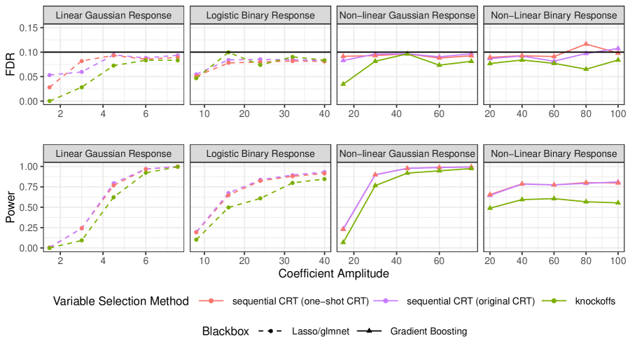
(a) $X$ follows a Gaussian AR model

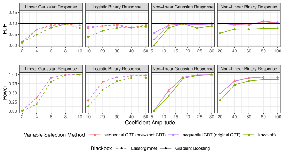
(b) $X$ follows an HMM

Figure 4: Performance of the sequential CRT with the original CRT and one-shot CRT (both use the symmetric statistic) and knockoffs on small synthetic datasets. The nominal false discovery rate level is 10%. Results are averaged over 100 independent experiments.

 

5.2 Comparison of the sequential CRT with knockoffs

We compare the proposed split version (Procedure 3) and symmetric statistic version (Procedure 4) of the sequential CRT with Model-X knockoffs. We run the sequential CRT with one-shot CRT. We consider similar settings as in the above Section 5.1. Since the computation time of one-shot CRT is much lower compared to the original CRT, here we run the experiments on larger datasets. In all settings in this section, the number of nonnulls is set to be 50. Other details can be found in Section 5.1 and Appendix A.2. Figure 5(a) compares the performance of the above methods in terms of empirical false discovery rate and power averaged over 100 independent replications. In all settings, the sequential CRT appears to control the FDR around the desired level $q=0.1$. In terms of power, the symmetric statistic version is comparable to knockoffs.

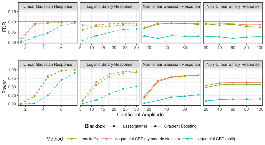
(a) $X$ follows a Gaussian AR model

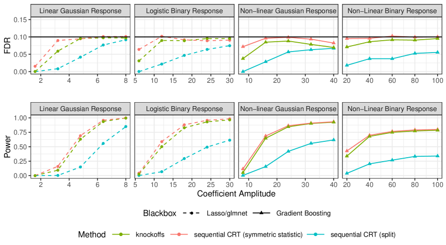
(b) $X$ follows an HMM

Figure 5: Performance of the proposed split version and symmetric statistic version of the sequential CRT compared to knockoffs on larger synthetic datasets. The nominal false discovery rate level is 10%. Results are averaged over 100 independent experiments.

 

5.3 The role of the number of potential discoveries

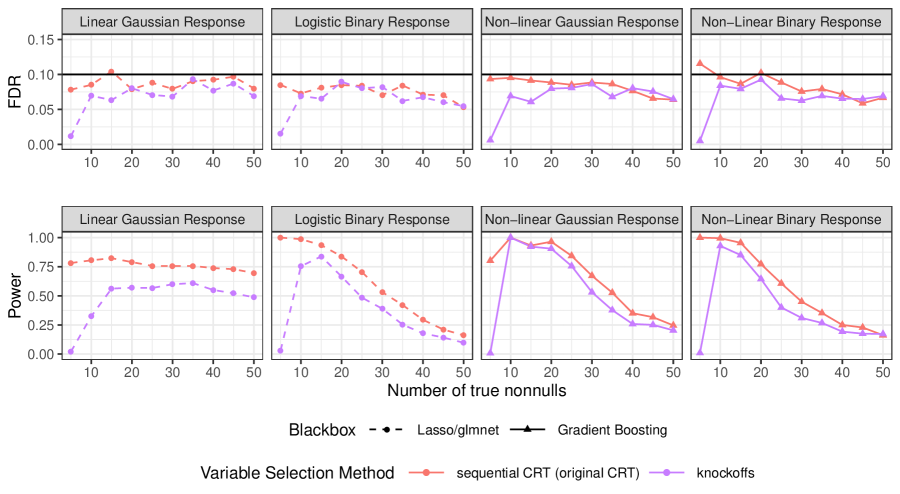
Figure 6: Performance of the sequential CRT compared to knockoffs as a function of the number of non-nulls. The nominal false discovery rate level is 10%. Results are averaged over 100 independent experiments.

Comparing the results from Sections 5.1 and 5.2, we observe that the power gain of the sequential CRT vis-a-vis model-X knockoffs is more noticeable when the number of nonnulls is small. To understand this phenomenon, return to the connection between the knockoff filter and Selective SeqStep+. It was shown by Barber and Candès [19] that the knockoff filter can be cast as a special case of the Selective SeqStep+ applied to “one-bit” p-values with $c$ chosen to be 0.5. When $q=0.1$ and $c=0.5$, the selected set of the Selective SeqStep+ becomes $\hat{\mathcal{S}}=\left\{j\leq\hat{k}:p_{j}\leq c\right\}$, where

$$\hat{k}=\max\left\{k\in\left\{1,\dots,p\right\}:\frac{1+\#\left\{j\leq k:p_{j}>0.5\right\}}{\#\left\{j\leq k:p_{j}\leq 0.5\right\}\vee 1}\leq 0.1\right\}.$$ (11)

When the number of nonnulls is small, the set above may be empty. Consider an example where the number of nonnulls is 8. Even in the ideal case where all the nonnulls have vanishing $p\operatorname{-values}$ and the nonnulls appear early in the sequence, for any $k\geq 8$, the left hand side in the inequality (11) becomes

$$\frac{1+\#\left\{\text{null }9\leq j\leq k:p_{j}\geq 0.5\right\}}{8+\#\left\{\text{null }9\leq j\leq k:p_{j}<0.5\right\}}\gtrsim\frac{1}{8}>0.1.$$ (12)

Therefore, most of the time there is no $k$ satisfying the inequality (11), thus we make no rejections. Hence the power will be low.

The sequential CRT, however, will not suffer from the same problem. We recall that throughout this paper, we take $c=0.1$ in the sequential CRT. With $c=0.1$, the definition of $\hat{k}$ becomes

$$\hat{k}=\max\left\{k\in\left\{1,\dots,p\right\}:\frac{1+\#\left\{j\leq k:p_{j}>0.1\right\}}{\#\left\{j\leq k:p_{j}\leq 0.1\right\}\vee 1}\leq 0.9\right\}.$$ (13)

With a good ordering the $p\operatorname{-values}$, the left hand side of the inequality can easily become lower than 0.9, a much less stringent threshold.

We run simulations varying the number of nonnulls. We compare the proposed symmetric statistic version of the sequential CRT with model-X knockoffs. We run the sequential CRT with one-shot CRT. We consider settings as in Section 5.1; details are in Appendix A.3. Figure 6 compares the performance of the above methods in terms of empirical false discovery rate and power averaged over 100 independent replications. In all settings, the sequential CRT appears to control the FDR around the desired level $q=0.1$. In terms of power, we see that the sequential CRT overcomes “the threshold phenomenon” discussed earlier.

5.4 Choice of the threshold $c$ and the number $B$ of randomizations

We here study the effect on power of the threshold $c$ and of the number $B$ of randomizations. We focus on the sequential CRT (symmetric statistics version with one-shot CRT). Intuitively, we expect the procedure with a smaller $c$ and a smaller $B$ to be more powerful. With a smaller $c$, our procedure is more likely to overcome “the threshold phenomenon” as discussed in Section 5.3. When using a smaller value of $B$, we make sure that we are not including too many irrelevant predictors in the machine learning algorithm while running the one-shot CRT algorithm. In addition, when we compute the statistics $z_{j}$ in Algorithm 4, we take the maximum (or the difference between the maximum and the median) of the feature importance statistics of $\mathbf{X}_{j},\mathbf{X}_{j}^{(1)},\dots,\mathbf{X}_{j}^{(B)}$; thus it is helpful to have a smaller $B$ so that the signal, i.e., the feature importance statistics of $\mathbf{X}_{j}$ has a chance of standing out. If we use an extremely large value of $B$, there is a chance that the maximum of the feature importance statistics of $\mathbf{X}_{j}^{(1)},\dots,\mathbf{X}_{j}^{(B)}$ exceeds that of $\mathbf{X}_{j}$. That said, $c$ and $B$ cannot be too small at the same time. At the very least, in order for our procedure to make any rejection, we need to have some $p\operatorname{-values}$ no larger than $c$. Since the $p\operatorname{-values}$ are bounded below by $1/(B+1)$, a necessary condition for not being powerless is to have $c\geq 1/(B+1)$.

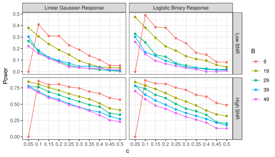
(a) Small datasets

 

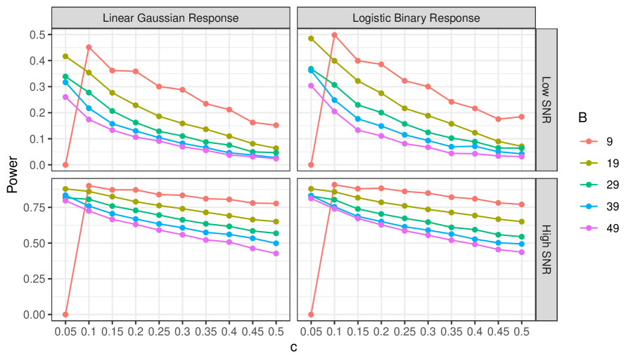
(b) Large datasets

Figure 7: Power of the sequential CRT (symmetric statistics version with one-shot CRT) with different choices of threshold $c$ and number of randomizations $B$. The nominal false discovery rate level is 10%. Results are averaged over 100 independent experiments.

The above heuristic arguments are confirmed in simulation studies. Figure 7 compares the performance of the sequential CRT with different values of $c$ and $B$. We consider several settings: linear/logistic models, small/large synthetic datasets, low/high signal to noise ratios. We observe the same phenomenon in all settings. Namely, power increases as $B$ decreases and $c$ decreases with the caveat that they cannot both be small at the same time. It appears that the pair $(B,c)=(9,0.1)$ is the most powerful in all settings, justifying the choices we made in earlier simulation studies. In Appendix A.4, we provide implementation details to reproduce Figure 7 and additionally show that the FDR is controlled at the nominal level for all choices of $B$ and $c$.

6 Real data application

We now apply our method to a breast cancer dataset to identify gene expressions on which the cancer stage depends. The dataset is from [21], which consists of $n=1,396$ staged cases of breast cancer. For each case, the data consists of expression level (mRNA) and copy number aberration (CNA) of $p=164$ genes. The goal is to identify genes whose expression level is not independent of the cancer stage, conditioning on all other genes and CNAs. The response variable, the progression stage of breast cancer, is binary. We take the dataset from [15] and pre-process the data as in their work. We refer to Section 5 and Section E of [15] for further details. Following [15], we model the distribution of expression levels using a multivariate Gaussian. The nominal false discovery rate is set to be 10%.

Below, we compare the following methods:

1. Sequential CRT: We consider Procedure 4 with one-shot CRT. We take the SeqStep threshold $c$ to be 0.1, and the number of randomizations to be 9. We take the importance statistics to be the absolute values of the coefficient of a cross-validated $L_{1}$-penalized logistic regression.

2. Distilled CRT [15]. We consider both $\operatorname{d}_{0}$CRT and $\operatorname{d}_{\operatorname{I}}$CRT; we refer to Section 2.3 and 2.4 of [15] for specific constructions of the dCRT. Since the response variable is binary, the distillation step is done by a cross-validated $L_{1}$-penalized logistic regression.

3. HRT [13]. Algorithm 1 of [13] is implemented with a logistic model fitted by a cross-validated $L_{1}$-penalized logistic regression and a data split of 50%-50%.

4. Knockoffs [7]. Knockoffs are constructed with the Gaussian semi-definite optimization algorithm. We take the feature importance statistic to be the glmnet coefficient difference.

For Distilled CRT and HRT, we reproduce the analysis from Liu et al. [15]. All methods considered above are randomized procedures, i.e., different runs of the same algorithm produce possibly different sets of discoveries. We run each method 100 times and compare the number of discoveries. Figure 8 is a boxplot showing the number of discoveries across random seeds. Our procedure appears to make more discoveries on average than the other methods. Compared to knockoffs, our procedure has less variability.

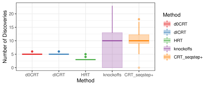
Figure 8: Number of discoveries on the breast cancer dataset

We present the full list of genes discovered by the sequential CRT in Table 2. Note here that the sequential CRT is random, thus different runs could produce different results. Following [7] and [2], to make the discoveries more “reliable”, we run the proposed method multiple times and only show the genes that are selected by our procedure more than 10% of the time. The 10% level is somewhat arbitrary and we do not make any claims about the discoveries exceeding this threshold. We leave the study of setting a threshold achieving theoretical error control guarantees to future research. We however observe that all discoveries above the 10% threshold were shown in other independent studies to be related to the development of cancer.

Selection frequency	Gene	Discovered by dCRT?	Confirmed in?
99%	HRAS	Yes	Geyer et al. [22]
99%	RUNX1	Yes	Li et al. [23]
96%	FBXW7	Yes	Liu et al. [24]
95%	GPS2	Yes	Huang et al. [25]
95%	NRAS		Galiè [26]
82%	FANCD2		Rudland et al. [27]
78%	MAP3K13	Yes	Han et al. [28]
76%	AHNAK		Chen et al. [29]
67%	MAP2K4		Liu et al. [30]
58%	CTNNA1		Clark et al. [31]
35%	NCOA3		Gupta et al. [32]
13%	LAMA2		Liang et al. [33]
10%	GATA3		Mehra et al. [34]

Table 2: Discoveries made by Procedure 4 on the breast cancer dataset

7 Discussion

Comparison with knockoffs

In this paper, we proposed a variable selection procedure, the sequential CRT. In comparison with model-X knockoffs, the proposed sequential CRT is generally more powerful than model-X knockoffs as shown in the simulation studies in Section 5. Specifically, we observe a much more noticeable power gain of the sequential CRT than is observed by model-X knockoffs when the number of nonnulls is small. In addition to the power gain, we note that the sequential CRT has another advantage over model-X knockoffs: it is usually easier to sample from the conditional distribution of $X_{j}\mid X_{-j}$ than to generate knockoffs, especially for complicated joint distribution of $X$.

Derandomizing the sequential CRT

Like many other Model-X procedures (e.g. Model-X knockoffs, distilled CRT, etc), the sequential CRT is a randomized procedure. In other words, different runs of the method produce might produce different selected sets. When the method is applied in practice, one would report those features whose selection frequency exceeds a threshold along with the corresponding frequencies. Ren et al. [17] studies the problem of derandomizing knockoffs. It will be interesting to study whether it is possible to derandomize the proposed method so that results are more consistent across different runs.

Theoretically validating power gains

While this paper demonstrates enhanced statistical power through simulations, it would be interesting to theoretically validate power gains. Intuitively, compared to Model-X knockoffs, the proposed method effectively reduces the number of covariates by a factor of 2 when computing feature importance statistics. It would be of interest to understand theoretically how important such reduction is in terms of statistical power.

Robustness to misspecification in the distribution of the covariates

Another interesting direction for future work is to study the robustness of the sequential CRT to misspecification in the distribution of the covariates. When the distribution of $X$ is known only approximately, Barber et al. [35] quantifies the possible FDR inflation of model-X knockoffs; and Berrett et al. [36] bounds the inflation in type-I error of the CRT. It will be interesting to evaluate the FDR inflation of the sequential CRT both empirically and theoretically.

Appendix A Simulation Details and Additional Simulation Studies

Software for our method is available from https://github.com/lsn235711/sequential-CRT, along with code to reproduce the analyses.

A.1 Details of the simulation study in Section 5.1

The samples are generated in the following way. In all examples, the samples are i.i.d. copies.

1. The explanatory variables $\mathbf{X}$ are generated from an AR(1) model with correlation parameter $\rho=0.5$.

   1. Conditional linear model with $n=300$ observations and $p=300$ variables. We set $Y=X^{\top}\beta+\epsilon$, where $\epsilon\sim\mathcal{N}(0,1)$. The vector $\beta$ has $20$ non-zero entries equal to $A/\sqrt{n}$, where the amplitude $A$ is a control parameter. The non-zero entries of $\beta$ are chosen at random.

   2. Conditional logistic model with $n=300$ observations and $p=300$ variables. $Y\mid X\sim\operatorname{Bern}\left(1/\left(1+\exp\left\{-X^{\top}\beta\right\}\right)\right)$. The vector $\beta$ has $20$ non-zero entries equal to $A/\sqrt{n}$, where the amplitude $A$ is a control parameter. The non-zero entries of $\beta$ are chosen at random.

   3. Conditional non-linear model with $n=500$ observations and $p=200$ variables. Conditional on $X$, $Y=\beta_{0}\sum_{k=1}^{10}\mathbbm{1}\left\{X_{j_{k}}>0\right\}\mathbbm{1}\left\{X_{\ell_{k}}>0\right\}+\epsilon$, where $\epsilon\sim\mathcal{N}(0,1)$ and $\beta_{0}=A/\sqrt{n}$. Again, $A$ is a control parameter. The two sets of indices in the regression function are each of cardinality 10 and disjoint. They are chosen uniformly at random.

   4. Conditional non-linear model with a binary response, and $n=500$ observations and $p=200$ variables. $Y\mid X\sim\operatorname{Bern}\left(1/\left(1+\exp\left\{-\tilde{X}^{\top}\beta\right\}\right)\right)$, where $\tilde{X}_{j}=\mathbbm{1}\left\{X_{j}>0\right\}-\mathbbm{1}\left\{X_{j}<0\right\}$. The vector $\beta$ has $20$ non-zero entries equal to $A/\sqrt{n}$, where $A$ is a control parameter. The non-zero entries of $\beta$ are chosen at random.

2. The explanatory variables $\mathbf{X}$ are generated from an HMM model. The HMM model considered has 5 hidden states and 3 output states. The transition matrix is

   $$\begin{bmatrix}0.6&0.1&0.1&0.1&0.1\\ 0.1&0.6&0.1&0.1&0.1\\ 0.1&0.1&0.6&0.1&0.1\\ 0.1&0.1&0.1&0.6&0.1\\ 0.1&0.1&0.1&0.1&0.6\\ \end{bmatrix}.$$

   The emission probability matrix is

   $$\begin{bmatrix}2/3&1/6&1/6\\ 5/12&5/12&1/6\\ 1/6&2/3&1/6\\ 1/6&5/12&5/12\\ 1/6&1/6&2/3\\ \end{bmatrix}.$$

   The initial probabilities are $[0.2,0.2,0.2,0.2,0.2]$.

   1. Conditional linear model with $n=300$ observations and $p=300$ variables. We set $Y=X^{\top}\beta+\epsilon$, where $\epsilon\sim\mathcal{N}(0,1)$. The vector $\beta$ has $20$ non-zero entries equal to $A/\sqrt{n}$, where the amplitude $A$ is a control parameter. The non-zero entries of $\beta$ are chosen at random.

   2. Conditional logistic model with $n=300$ observations and $p=300$ variables. $Y\mid X\sim\operatorname{Bern}\left(1/\left(1+\exp\left\{-(X-2\cdot\mathbf{1})^{\top}\beta\right\}\right)\right)$. The vector $\beta$ has $20$ non-zero entries equal to $A/\sqrt{n}$, where the amplitude $A$ is a control parameter. The non-zero entries of $\beta$ are chosen at random.

   3. Conditional non-linear model with $n=500$ observations and $p=200$ variables. Conditional on $X$, $Y=\beta_{0}\sum_{k=1}^{10}\mathbbm{1}\left\{X_{j_{k}}>1.5\right\}\mathbbm{1}\left\{X_{\ell_{k}}>1.5\right\}+\epsilon$, where $\epsilon\sim\mathcal{N}(0,1)$ and $\beta_{0}=A/\sqrt{n}$. Again, $A$ is a control parameter. The two sets of indices in the regression function are each of cardinality 10 and disjoint. They are chosen uniformly at random.

   4. Conditional non-linear model with a binary response, and $n=500$ observations and $p=200$ variables. $Y\mid X\sim\operatorname{Bern}\left(1/\left(1+\exp\left\{-\tilde{X}^{\top}\beta\right\}\right)\right)$, where $\tilde{X}_{j}=\mathbbm{1}\left\{X_{j}>1.5\right\}-2/3$. The vector $\beta$ has $20$ non-zero entries equal to $A/\sqrt{n}$, where $A$ is a control parameter. The non-zero entries of $\beta$ are chosen at random.

We set the FDR threshold to be $q=0.1$. We take $c=0.1$ in Selective SeqStep+. The number of randomizations $B$ in Procedure 3 and 4 are set to be $9$. To compute feature importance, the details of the blackbox algorithm we used are as follows: for lasso/glmnet, the regularization parameter is chosen using cross validation; for gradient boosting, we use the R-package XGBoost. We set the parameters eta=0.05, max_depth=2, nrounds = 100.

A.2 Details of the simulation study in Section 5.2

The samples are generated in the same way as in Section A.1, however, with a larger number of observations $n$, a larger number of variables $p$, and a larger number of nonnulls $k$. The methods are also the same as in A.1. With the same labeling as before, we set the parameters as follows.

1. For the AR(1) model:

   1. $n=1000$, $p=1000$, and $k=50$;

   2. $n=1000$, $p=1000$, and $k=50$;

   3. $n=1200$, $p=500$, and $k=50$;

   4. $n=1200$, $p=500$, and $k=50$.

2. For the HMM model:

   1. $n=1000$, $p=1000$, and $k=50$.

   2. $n=1000$, $p=1000$, and $k=50$.

   3. $n=1200$, $p=500$, and $k=50$.

   4. $n=1200$, $p=500$, and $k=50$.

A.3 Details of the simulation study in Section 5.3

The samples are generated in the same way as in Section A.1, however, with a fixed control parameter $A$, and a varying number of nonnulls $k\in\left\{5,10,\dots,50\right\}$. The methods are also the same as in A.1 and we only consider the AR(1) model. With the same labeling as before, we set the parameters as follows: (a) $A=1.5$; (b) $A=8$; (c) $A=15$; (d) $A=20$.

A.4 Details of the simulation study in Section 5.4

The FDR threshold is set to be $q=0.1$. To compute feature importance statistic, we use lasso for the linear case and glmnet for the logistic case, where the regularization parameter is chosen using cross validation. For the “small dataset” setting, the samples are generated in the same way as in Section A.1. We only consider the AR(1) model. We fix the control parameter $A$ as follows:

linear, low SNR	linear, high SNR	logistic, low SNR	logistic high SNR
$A=3.5$	$A=5$	$A=12$	$A=30$

For the “large dataset” setting, the samples are generated in the same way as in Section A.2. We only consider the AR(1) model. We fix the control parameter $A$ as follows:

linear, low SNR	linear, high SNR	logistic, low SNR	logistic high SNR
$A=3.5$	$A=5$	$A=10$	$A=20$

Figure 9 compares the performance of the sequential CRT (one-shot version) in terms of the FDR with various different values of $c$ and $B$. It appears that the FDR is well controlled for all combinations of $c$ and $B$.

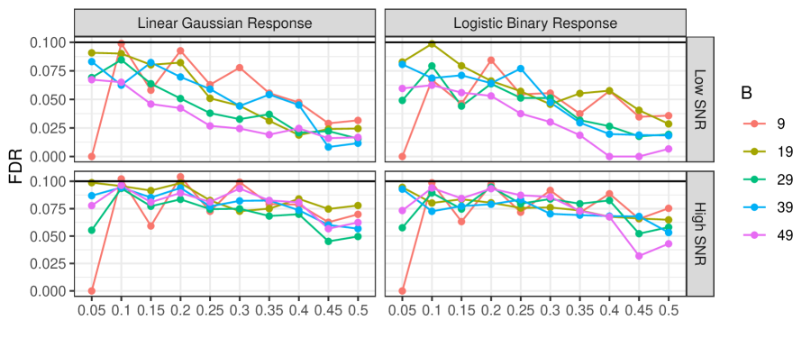
(a) Small datasets

 

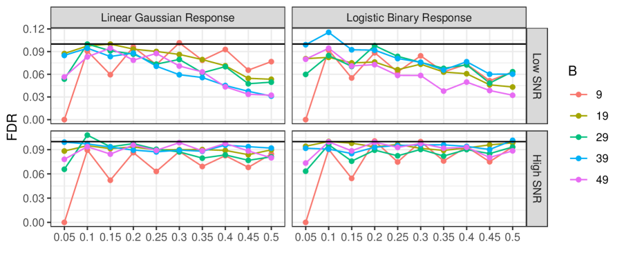
(b) Large datasets

Figure 9: FDR of the sequential CRT (one-shot) with different choices of threshold $c$ and number of randomizations $B$. The nominal false discovery rate level is 10%. Results are averaged over 100 independent experiments.

A.5 Implementation details of Table 1

The explanatory variables $\mathbf{X}$ are generated from an AR(1) model with correlation parameter $\rho=0.5$. Other details are as in Section A.1.

A.6 Implementation details of Figure 2

We simulate $n=200$ observations and $p=120$ variables. The explanatory variables $\mathbf{X}$ are jointly Gaussian with mean $0$ and variance $\Sigma$. $\Sigma$ is a block diagonal matrix with block size $3$. The non-zero off-diagonal entries of $\Sigma$ are equal to 0.3. Conditional on $X$, $Y=X^{\top}\beta+\epsilon$, where $\epsilon\sim\mathcal{N}(0,1)$. The vector $\beta$ has $30$ non-zero entries equal to $3/\sqrt{n}$. The non-zero entries of $\beta$ are chosen at random. The $p\operatorname{-values}$ are obtained using Algorithm 1 where the test statistics are computed using the lasso. The number of randomizations $B$ is set to $19$. We set $q=0.1$ and $c=0.3$. Each $a_{j}$ is estimated as an average of 5000 binary variables. The histogram (Figure 2) is based on 500 samples.

A.7 Comparison of the Sequential CRT with other benchmark methods

We compare the proposed split version (Procedure 3) and symmetric statistic version (Procedure 4) of the sequential CRT with the following methods:

1. Knockoffs [Candès et al., 2018]. Knockoffs are constructed with the Gaussian semi-definite optimization algorithm. We take the feature importance statistic to be the glmnet coefficient difference.

2. Distilled CRT [Liu et al., 2022]. We consider both $\operatorname{d}_{0}$CRT and $\operatorname{d}_{\operatorname{I}}$CRT; we refer to Section 2.3 and 2.4 of [Liu et al., 2022] for specific constructions of the dCRT. In the continuous response case, the distillation step is done by a cross-validated lasso; in the binary response case, the distillation step is done by $L_{1}$-penalized logistic regression.

3. HRT [Tansey et al., 2021]. We implement Algorithm 1 of [Tansey et al., 2021] with a data split of 50%-50%. In the continuous response case, the algorithm is implemented with a cross-validated lasso; in the binary response case, it is implemented with a cross-validated $L_{1}$-penalized logistic regression.

4. Gaussian Mirror [Xing et al., 2019]. We implement the Gaussian Mirror with the gm() function in the GM package (https://github.com/BioAlgs/GM).

We run the sequential CRT with one-shot CRT. We consider similar settings as in Section 5.2, and focus on the settings of AR model with a conditional linear model and AR model with a conditional logistic model. Other details can be found in Section 5.2 and Appendix A.2. Figure 10 compares the performance of the above methods in terms of empirical false discovery rate and power averaged over 100 independent replications. The sequential CRT (symmetric statistics) appears to have the highest power among all methods. In terms of the false discovery rate, all methods except the gaussian mirror control the false discovery rate at the desired level. The gaussian mirror appears to have a huge FDR inflation when the signal to noise ratio is small. Hence, from a practical point of view, it may not the most appealing method when we have no prior information on the signal strength.

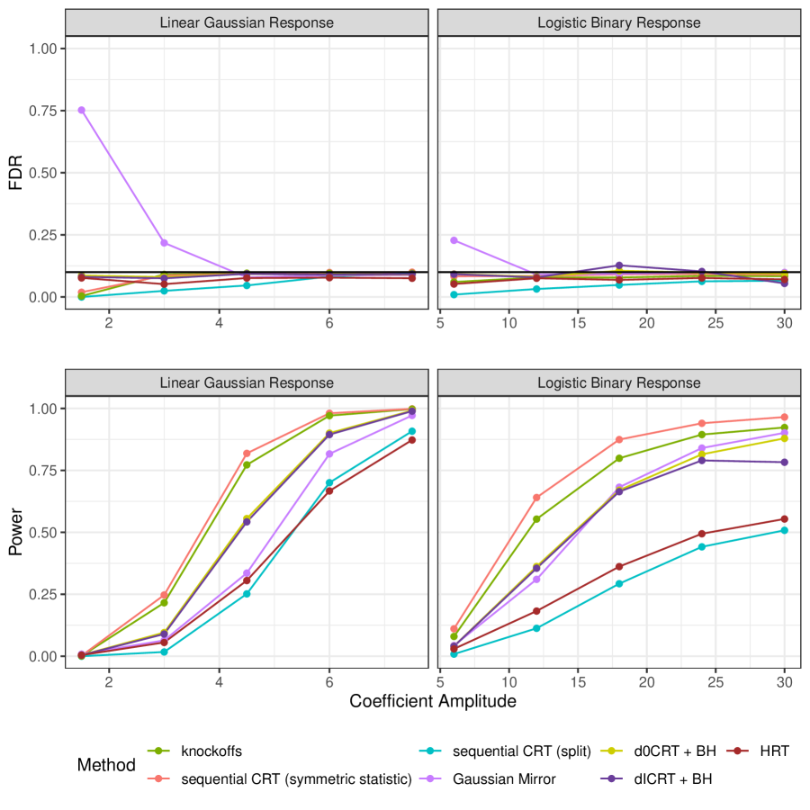
Figure 10: Performance of the proposed split version and symmetric statistic version of the sequential CRT compared to other benchmarks on synthetic datasets. The nominal false discovery rate level is 10%. Results are averaged over 100 independent experiments.

Appendix B Proofs

B.1 Proof of Theorem 4

For the sake of notation, we write $m=p$, i.e. we let $m$ be the number of hypotheses/variables, to distinguish from the “p” in $p\operatorname{-values}$: $p_{1},p_{2},$ etc.

B.1.1 Proof of upper bound (5)

To bound the FDR, we modify arguments from the proof of Lemma 1 and Theorem 3 in Supplement of [Barber and Candès, 2015]. We include a part of the statement in [Barber and Candès, 2015, Lemma 1] for reference:

“For $k=m,m-1,\ldots,1,0,$ put $V^{+}(k)=$ $\#\left\{j\in\mathcal{H}_{0}:1\leq j\leq k,p_{j}\leq c\right\}$ and $V^{-}(k)=\#\{j\in\mathcal{H}_{0}:1\leq j\leq k,p_{j}>c\}$ with the convention that $V^{\pm}(0)=0.$ Let $\mathcal{F}_{k}$ be the filtration defined by knowing all the nonnull $p\operatorname{-values}$, as well as $V^{\pm}\left(k^{\prime}\right)$ for all $k^{\prime}\geq k.$ Then the process

$$M(k)=\frac{V^{+}(k)}{1+V^{-}(k)}$$

is a super-martingale running backward in time with respect to $\mathcal{F}_{k}$.”

The conclusion above assumes that the null $p$ -values are i.i.d., satisfy $p_{j}\geq$ Unif[0,1], and are independent from the nonnulls. Here, we are no longer in the i.i.d. setting of [Barber and Candès, 2015, Lemma 1]. Yet, the same proof goes through with exchangeability. This mean that the above result still holds under the conditions that the null $p\operatorname{-values}$ are exchangeable given nonnull $p\operatorname{-values}$ and that marginally, null $p\operatorname{-values}$ satisfy $p_{j}\geq$ Unif[0,1].

As in [Barber and Candès, 2015], the $\hat{k}$ defined in (3) is a stopping time with respect to the backward filtration $\left\{\mathcal{F}_{k}\right\}$ since $\{\hat{k}\geq k\}\in\mathcal{F}_{k}$. By the optional stopping time theorem for super-martingales,

$$\mathbb{E}\left[M(\hat{k})\big{|}\mathcal{F}_{m}\right]\leq M(m)=\frac{\#\left\{j\in\mathcal{H}_{0}:p_{j}\leq c\right\}}{1+\#\left\{j\in\mathcal{H}_{0}:p_{j}>c\right\}}.$$

As in [Barber and Candès, 2015], we write $V=\#\left\{j\in\mathcal{H}_{0},j\leq\hat{k}:p_{j}\leq c\right\}$ and $R=\#\left\{j\leq\hat{k}:p_{j}\leq c\right\}$.

$$\mathbb{E}\left[\operatorname{FDP}|\mathcal{F}_{m}\right] =\mathbb{E}\left[\frac{V}{R\vee 1}\Big{|}\mathcal{F}_{m}\right]=\mathbb{E}\left[\frac{V}{R\vee 1}\cdot\mathbbm{1}\left\{\hat{k}>0\right\}\Big{|}\mathcal{F}_{m}\right]$$

$$=\mathbb{E}\left[\frac{\#\left\{j\in\mathcal{H}_{0},j\leq\hat{k}:p_{j}\leq c\right\}}{1+\#\left\{j\in\mathcal{H}_{0},j\leq\hat{k}:p_{j}>c\right\}}\cdot\left(\frac{1+\#\left\{j\in\mathcal{H}_{0},j\leq\hat{k}:p_{j}>c\right\}}{\#\left\{j\leq\hat{k}:p_{j}\leq c\right\}\vee 1}\cdot\mathbbm{1}\left\{\hat{k}>0\right\}\right)\Bigg{|}\mathcal{F}_{m}\right]$$

$$\leq\left(\mathbb{E}\left[\frac{\#\left\{j\in\mathcal{H}_{0},j\leq\hat{k}:p_{j}\leq c\right\}}{1+\#\left\{j\in\mathcal{H}_{0},j\leq\hat{k}:p_{j}>c\right\}}\Bigg{|}\mathcal{F}_{m}\right]\cdot\frac{1-c}{c}\cdot q\right)\wedge 1$$

$$\leq\left(\frac{\#\left\{j\in\mathcal{H}_{0}:p_{j}\leq c\right\}}{1+\#\left\{j\in\mathcal{H}_{0}:p_{j}>c\right\}}\cdot\frac{1-c}{c}\cdot q\right)\wedge 1$$

$$\leq\left(\frac{\#\left\{j\in\mathcal{H}_{0}:p_{j}\leq c\right\}}{1+\#\left\{j\in\mathcal{H}_{0}:p_{j}>c\right\}}\wedge\frac{c}{(1-c)q}\right)\frac{1-c}{c}q.$$

This implies that

$$\operatorname{FDR} =\mathbb{E}\left[\mathbb{E}\left[\operatorname{FDP}|\mathcal{F}_{m}\right]\right]\leq\frac{1-c}{c}q\mathbb{E}\left[\left(\frac{\#\left\{j\in\mathcal{H}_{0}:p_{j}\leq c\right\}}{1+\#\left\{j\in\mathcal{H}_{0}:p_{j}>c\right\}}\wedge\frac{c}{(1-c)q}\right)\right]$$

$$=\frac{(1-c)q}{c}\sum_{k=0}^{m}\pi_{k}\left(\frac{k}{1+m-k}\wedge\frac{c}{(1-c)q}\right),$$

where $\pi_{k}=\mathbb{P}\left[\#\left\{i\in\mathcal{H}_{0}:p_{i}\leq c\right\}=k\right]$.

Thus, bounding the FDR reduces to an optimization problem:

$$\text{maximize}_{\pi_{k}}\quad \sum_{k=0}^{m}\pi_{k}\left(\frac{k}{1+m-k}\wedge\frac{c}{(1-c)q}\right)$$ (14)

subject to $$\sum\pi_{k}=1,\pi_{k}\geq 0,\sum k\pi_{k}\leq cm.$$

More rigorously, let $V_{\operatorname{opt}}$ be the optimal value of (14). Then our previous analysis implies that $\operatorname{FDR}\leq\frac{(1-c)q}{c}V_{\operatorname{opt}}$. Note that with $\pi_{k}=\mathbb{P}\left[\#\left\{i\in\mathcal{H}_{0}:p_{i}\leq c\right\}=k\right]$, we have $\sum k\pi_{k}\leq c$ since $\sum k\pi_{k}=\mathbb{E}\left[\#\left\{i\in\mathcal{H}_{0}:p_{i}\leq c\right\}\right]=\sum_{i\in\mathcal{H}_{0}}\mathbb{P}\left[p_{i}\leq c\right]\leq cm$.

It remains to solve (14). The optimal value of (14) is indeed the same as that of (15):

$$\text{maximize}_{\pi_{k}}\quad \sum_{k=0}^{m^{\prime}}\pi_{k}\left(\frac{k}{1+m-k}\right)$$ (15)

subject to $$\sum_{k=0}^{m^{\prime}}\pi_{k}=1,\pi_{k}\geq 0,\sum_{k=0}^{m^{\prime}}k\pi_{k}\leq cm,$$

where $m^{\prime}=\lfloor\frac{cm}{q+c(1-q)}\rfloor$. This is because for $k>m^{\prime}$, $\frac{k}{1+m-k}>\frac{c}{(1-c)q}$. Hence for any optimal solution of (14) such that $\pi_{k}>0$ for some $k>m^{\prime}$, we can move the mass to $m^{\prime}$, i.e., define $\pi^{\prime}_{m^{\prime}}=\sum_{k\geq m^{\prime}}\pi_{k}$. Then the new $\pi^{\prime}$ still satisfies the constraints in (14) and achieves the same objective value.

To solve (15), note that since $\frac{k}{1+m-k}$ is convex in $k$, and the constraints are linear in $k$, the optimal value is achieved when the probability $\pi$ has its mass on the boundary. Formally, the optimal value is achieved when $\pi_{k}=0$ for all $k$ except for $0$ and $m^{\prime}$. To see this, assume that there is a $k_{0}\neq 0,m^{\prime}$ such that $\pi_{k_{0}}\neq 0$. We will see that if we move the mass at $k_{0}$ to $0$ and $m^{\prime}$, then the constraints are still satisfied but the objective function will have a larger value. More precisely, if we define $\tilde{\pi}$ by taking $\tilde{\pi}_{0}=\pi_{0}+\pi_{k_{0}}(m^{\prime}-k_{0})/m^{\prime}$, $\tilde{\pi}_{m^{\prime}}=\pi_{m^{\prime}}+\pi_{k_{0}}k_{0}/m^{\prime}$, and $\tilde{\pi}_{k_{0}}=0$, then $\sum_{k=0}^{m^{\prime}}\tilde{\pi}_{k}=\sum_{k=0}^{m^{\prime}}\pi_{k}=1$, and $\sum_{k=0}^{m^{\prime}}k\tilde{\pi}_{k}=\sum_{k=0}^{m^{\prime}}k\pi_{k}\leq cm$. The objective function $\sum_{k=0}^{m^{\prime}}\tilde{\pi}_{k}\left(\frac{k}{1+m-k}\right)>\sum_{k=0}^{m^{\prime}}\pi_{k}\left(\frac{k}{1+m-k}\right)$, because $\frac{k}{1+m-k}$ is strictly convex in $k$.

Therefore the optimal value of (15) is achieved when $\pi_{k}=0$ for all $k$ except for $0$ and $m^{\prime}$. Thus the optimal value $V_{\operatorname{opt}}=\frac{\pi_{m^{\prime}}m^{\prime}}{1+m-m^{\prime}}$, where $m^{\prime}\pi_{m^{\prime}}=cm$. As $m^{\prime}=\lfloor\frac{cm}{q+c(1-q)}\rfloor\leq\frac{cm}{q+c(1-q)}$, we have

$$V_{\operatorname{opt}}=\frac{\pi_{m^{\prime}}m^{\prime}}{1+m-m^{\prime}}\leq\frac{cm}{1+m-\frac{cm}{q+c(1-q)}}\leq\frac{c(q+c(1-q))}{q(1-c)}.$$

Hence

$$\operatorname{FDR}\leq\frac{(1-c)q}{c}\frac{c(q+c(1-q))}{q(1-c)}=q+c(1-q).$$

B.1.2 Proof of upper bound (6)

We work here with the additional constraint that for pairs of nulls $(i,j)$, $\operatorname{Corr}\left[\mathbbm{1}\left\{p_{i}\leq c\right\},\left\{p_{j}\leq c\right\}\right]\leq\rho$. Put $c_{0}=\mathbb{P}\left[p_{i}\leq c\right]$ and $m_{0}=\#\left\{i\in\mathcal{H}_{0}\right\}$. Then $\operatorname{Cov}\left[\mathbbm{1}\left\{p_{i}\leq c\right\},\left\{p_{j}\leq c\right\}\right]\leq\rho c_{0}(1-c_{0})$. Also,

$$\operatorname{Var}\left[\#\left\{i\in\mathcal{H}_{0}:p_{i}\leq c\right\}\right] =m_{0}\operatorname{Var}\left[\mathbbm{1}\left\{p_{i}\leq c\right\}\right]+m_{0}(m_{0}-1)\operatorname{Cov}[\mathbbm{1}\left\{p_{i}\leq c\right\},\mathbbm{1}\left\{p_{j}\leq c\right\}]$$

$$\leq m_{0}(1+\rho(m_{0}-1))c_{0}(1-c_{0}).$$

Alternatively, we can write the variance as a function of the $\pi_{k}$’s:

$$\operatorname{Var}\left[\#\left\{i\in\mathcal{H}_{0}:p_{i}\leq c\right\}\right]=\sum_{k=0}^{m}(k-c_{0}m_{0})^{2}\pi_{k}.$$

Thus the constraint that $\operatorname{Corr}\left[\mathbbm{1}\left\{p_{i}\leq c\right\},\left\{p_{j}\leq c\right\}\right]\leq\rho$ can be rewritten as

$$\sum_{k=0}^{m}(k-c_{0}m_{0})^{2}\pi_{k}\leq m_{0}(1+\rho(m_{0}-1))c_{0}(1-c_{0}).$$

Following the analysis in Section B.1.1, bounding the FDR reduces to solving an optimization problem with decision variables $\{\pi_{k}\}$, $m_{0}$ and $c_{0}$:

maximize $$\sum_{k=0}^{m}\pi_{k}\left(\frac{k}{1+m-k}\wedge\frac{c}{(1-c)q}\right)$$ (16)

subject to $$\sum_{k=0}^{m}\pi_{k}=1,\pi_{k}\geq 0,\,\,\sum_{k=0}^{m}\pi_{k}=c_{0}m_{0},\,\,c_{0}\leq c,\,\,m_{0}\leq m,$$

$$\sum_{k=0}^{m}(k-c_{0})^{2}\pi_{k}\leq m_{0}(1+\rho(m_{0}-1))c_{0}(1-c_{0}).$$

Specifically, $\operatorname{FDR}\leq\frac{(1-c)q}{c}V_{\operatorname{opt}}\eqref{eqn:opt1}$, where $V_{\operatorname{opt}}\eqref{eqn:opt1}$ is the optimal value of the program (16). The optimization problem is equivalent (in the sense that $V_{\operatorname{opt}}\eqref{eqn:opt1}=V_{\operatorname{opt}}\eqref{eqn:opt2}$) to:

maximize $$\sum_{k=0}^{m^{\prime}}\pi_{k}\left(\frac{k}{1+m-k}\right)$$ (17)

subject to $$\sum_{k=0}^{m^{\prime}}\pi_{k}=1,\,\,\pi_{k}\geq 0,\,\,\sum_{k=0}^{m^{\prime}}\pi_{k}=c_{0}m_{0},\,\,c_{0}\leq c,m_{0}\leq m,$$

$$\sum_{k=0}^{m^{\prime}}(k-c_{0})^{2}\pi_{k}\leq m_{0}(1+\rho(m_{0}-1))c_{0}(1-c_{0}),$$

where $m^{\prime}=\lfloor\frac{cm}{q+c(1-q)}\rfloor$. For now, fix $\sigma>0$ and $c_{1}\leq c$ and focus on the case where $\sum_{k=0}^{m^{\prime}}(k-c_{0})^{2}\pi_{k}=m^{2}\sigma^{2}$ and $\sum_{k=0}^{m}\pi_{k}=c_{1}m=c_{0}m_{0}$. We will optimize over the choice of $\sigma$ and $c_{1}$ later. That is, consider

maximize $$\sum_{k=0}^{m^{\prime}}\pi_{k}\left(\frac{k}{1+m-k}\right)$$ (18)

subject to $$\sum_{k=0}^{m^{\prime}}\pi_{k}=1,\pi_{k}\geq 0,\sum_{k=0}^{m^{\prime}}\pi_{k}=c_{1}m,$$

$$\sum_{k=0}^{m^{\prime}}(k-c_{1})^{2}\pi_{k}=\sigma^{2}m^{2},$$

with decision variables $\{\pi_{k}\}$. $V_{\operatorname{opt}}\eqref{eqn:opt3}$ is a function of $\sigma$, $c_{0}$ and $m_{0}$ and we have:

$$V_{\operatorname{opt}}\eqref{eqn:opt2}=\max\left\{V_{\operatorname{opt}}\eqref{eqn:opt3}:\sigma^{2}\leq m_{0}(1+\rho(m_{0}-1))c_{0}(1-c_{0})/m^{2},c_{0}\leq c,m_{0}\leq m\right\}.$$ (19)

As for the optimization problem (18), this is an LP with three equality constraints. By Carathéodory’s theorem, any optimal solution must have at most three non-zero $\pi_{k}$’s. Hence, the problem becomes ($V_{\operatorname{opt}}\eqref{eqn:opt3}=V_{\operatorname{opt}}\eqref{eqn:opt4}$)

maximize $$\pi_{1}\frac{k_{1}}{1+m-k_{1}}+\pi_{2}\frac{k_{2}}{1+m-k_{2}}+\pi_{3}\frac{k_{3}}{1+m-k_{3}}$$ (20)

subject to $$\pi_{1}+\pi_{2}+\pi_{3}=1,\,(\pi_{1},\pi_{2},\pi_{3})\geq 0,$$

$$\pi_{1}k_{1}+\pi_{2}k_{2}+\pi_{3}k_{3}=c_{1}m,$$

$$\pi_{1}(k_{1}-c_{1})^{2}+\pi_{2}(k_{2}-c_{1})^{2}+\pi_{3}(k_{3}-c_{1})^{2}=\sigma^{2}m^{2},$$

$$(k_{1},k_{2},k_{3})\leq\lfloor\frac{cm}{q+c(1-q)}\rfloor,$$

where the last inequality says that all components of the left-hand side are upper bounded by the right-hand side. Set $x_{i}=k_{i}/m$, $1\leq i\leq 3$, and relax the constraints by allowing $x_{1}$ to take any real value in the interval. We also increase the objective for simplification and consider

maximize $$\pi_{1}\frac{x_{1}}{1-x_{1}}+\pi_{2}\frac{x_{2}}{1-x_{2}}+\pi_{3}\frac{x_{3}}{1-x_{3}}\quad$$ (21)

subject to $$\pi_{1}+\pi_{2}+\pi_{3}=1,$$

$$\pi_{1}x_{1}+\pi_{2}x_{2}+\pi_{3}x_{3}=c_{1},$$

$$\pi_{1}(x_{1}-c_{1})^{2}+\pi_{2}(x_{2}-c_{1})^{2}+\pi_{3}(x_{3}-c_{1})^{2}=\sigma^{2},$$

$$(\pi_{1},\pi_{2},\pi_{3})\geq 0,\,\,0\leq(x_{1},x_{2},x_{3})\leq\frac{c}{q+c(1-q)},$$

so that $V_{\operatorname{opt}}\eqref{eqn:opt4}\leq V_{\operatorname{opt}}\eqref{eqn:opt5}$. By lemma 1,

$$V_{\operatorname{opt}}\eqref{eqn:opt5}\leq\frac{\alpha}{1-\alpha}-\frac{(\alpha-c_{1})^{2}}{(1-\alpha)(\sigma^{2}+(1-c_{1})(\alpha-c_{1}))},$$

where $\alpha=\frac{c}{q+c(1-q)}$. The upper bound is clearly an increasing function of $\sigma^{2}$ and $c_{1}$. Hence, for any $\sigma^{2}\leq m_{0}(1+\rho(m_{0}-1))c_{0}(1-c_{0})/m^{2}\leq(1+\rho(m-1))/mc_{0}(1-c_{0})$ and any $c_{1}=c_{0}m_{0}/m\leq c_{0}$,

$$V_{\operatorname{opt}}\eqref{eqn:opt5} \leq\frac{\alpha}{1-\alpha}-\frac{(\alpha-c_{1})^{2}}{(1-\alpha)(\sigma^{2}+(1-c_{1})(\alpha-c_{1}))}$$

$$\leq\frac{\alpha}{1-\alpha}-\frac{(\alpha-c_{0})^{2}}{(1-\alpha)(\tilde{\rho}c_{0}(1-c_{0})+(1-c_{0})(\alpha-c_{0}))},$$

where $\tilde{\rho}=((m-1)\rho+1)/m$. As

$$\frac{d}{dc_{0}}\frac{(\alpha-c_{0})^{2}}{(\tilde{\rho}c_{0}(1-c_{0})+(1-c_{0})(\alpha-c_{0}))}=-\frac{(\alpha-c_{0})(1-\alpha)+\tilde{\rho}(\alpha+c_{0}-2\alpha c_{0}))}{(c_{0}-1)^{2}(\alpha+c_{0}\rho-c_{0})^{2}}<0,$$

the bound $\frac{\alpha}{1-\alpha}-\frac{(\alpha-c_{0})^{2}}{(1-\alpha)(\tilde{\rho}c_{0}(1-c_{0})+(1-c_{0})(\alpha-c_{0}))}$ is an increasing function of $c_{0}$. Hence for any $c_{0}\leq c$,

$$V_{\operatorname{opt}}\eqref{eqn:opt5} \leq\frac{\alpha}{1-\alpha}-\frac{(\alpha-c_{0})^{2}}{(1-\alpha)(\tilde{\rho}c_{0}(1-c_{0})+(1-c_{0})(\alpha-c_{0}))}$$

$$\leq\frac{\alpha}{1-\alpha}-\frac{(\alpha-c)^{2}}{(1-\alpha)(\tilde{\rho}c(1-c)+(1-c)(\alpha-c))}.$$

Together with (19), this implies that

$$V_{\operatorname{opt}}\eqref{eqn:opt1} \leq\frac{\alpha}{1-\alpha}-\frac{(\alpha-c)^{2}}{(1-\alpha)(\tilde{\rho}c(1-c)+(1-c)(\alpha-c))},$$

where $\alpha=\frac{c}{q+c(1-q)}$, $\tilde{\rho}=((m-1)\rho+1)/m$. Thus

$$\operatorname{FDR} \leq\frac{(1-c)q}{c}V_{\operatorname{opt}}\eqref{eqn:opt1}\leq\frac{(1-c)q}{c}\left(\frac{\alpha}{1-\alpha}-\frac{(\alpha-c)^{2}}{(1-\alpha)(\tilde{\rho}c(1-c)+(1-c)(\alpha-c))}\right)$$

$$=q+\frac{\tilde{\delta}}{1+\beta\tilde{\delta}}\left[\frac{c}{1-c}-\frac{c-c\tilde{\delta}}{1-(c-c\tilde{\delta})}q\right],$$

where $\tilde{\rho}=\frac{(m-1)\rho+1}{m}$, $\beta=\frac{c+(1-c)q}{(1-c)(1-q)}$, and $\tilde{\delta}=\tilde{\rho}\frac{c(1-q)+q}{c(1-q)}$. Upon setting $\delta=\rho\frac{c(1-q)+q}{c(1-q)}$, $\tilde{\delta}\leq\delta$, whence,

$$\operatorname{FDR}\leq q+\frac{\tilde{\delta}}{1+\beta\tilde{\delta}}\left[\frac{c}{1-c}-\frac{c-c\tilde{\delta}}{1-(c-c\tilde{\delta})}q\right]\leq q+\frac{\delta}{1+\beta\delta}\left[\frac{c}{1-c}-\frac{c-c\delta}{1-(c-c\delta)}q\right].$$

Lemma 1.

Fix $1>\alpha>c>0$. The problem

maximize $$\pi_{1}\frac{x_{1}}{1-x_{1}}+\pi_{2}\frac{x_{2}}{1-x_{2}}+\pi_{3}\frac{x_{3}}{1-x_{3}}\quad$$ (22)

subject to $$\pi_{1}+\pi_{2}+\pi_{3}=1,$$

$$\pi_{1}x_{1}+\pi_{2}x_{2}+\pi_{3}x_{3}=c,$$

$$\pi_{1}(x_{1}-c)^{2}+\pi_{2}(x_{2}-c)^{2}+\pi_{3}(x_{3}-c)^{2}=\sigma^{2},$$

$$(\pi_{1},\pi_{2},\pi_{3})\geq 0,\,\,(x_{1},x_{2},x_{3})\leq\alpha,$$

has optimal value

$$V_{\operatorname{opt}}=\frac{\alpha}{1-\alpha}-\frac{(\alpha-c)^{2}}{(1-\alpha)(\sigma^{2}+(1-c)(\alpha-c))}.$$

Proof.

Let $\pi^{\star}$ and $x^{\star}$ be an optimal solution with objective value $V_{\operatorname{opt}}$. If $\pi_{i}^{\star}>0$ and $x_{i}^{\star}<\alpha$ for all $i=1,2,3$, then by complementary slackness, there exist $\lambda$ and $\gamma$ such that

$$\frac{\pi^{\star}_{i}}{(1-x_{i}^{\star})^{2}}+\lambda\pi_{i}^{\star}+\gamma\pi_{i}^{\star}(2x_{i}^{\star}-c)=0$$

holds for $i=1,2,3$. This further implies that

$$\frac{1}{(1-x_{i}^{\star})^{2}}+\lambda+\gamma(2x_{i}^{\star}-c)=0.$$

The left-hand side is strictly convex in $x$, thus this equation has at most two distinct solutions for $x$. Thus any optimal solution of (22) either has some $x_{i}$’s taking on the value $\alpha$ or two $x_{i}$’s are the same. We analyze each case below.

Optimal solution has some entries taking on the value $\alpha$.

Without loss of generality, assume that the optimal solution has $x_{3}=\alpha$. Then (22) is equivalent to

maximize $$\pi_{1}\frac{x_{1}}{1-x_{1}}+\pi_{2}\frac{x_{2}}{1-x_{2}}+\pi_{3}\frac{\alpha}{1-\alpha}\quad$$

subject to $$\pi_{1}+\pi_{2}+\pi_{3}=1,$$

$$\pi_{1}x_{1}+\pi_{2}x_{2}+\pi_{3}\alpha=c,$$

$$\pi_{1}(x_{1}-c)^{2}+\pi_{2}(x_{2}-c)^{2}+\pi_{3}(\alpha-c)^{2}=\sigma^{2},$$

$$(\pi_{1},\pi_{2},\pi_{3})\geq 0,\,\,(x_{1},x_{2})\leq\alpha.$$

Write $\pi_{3}=1-\pi_{1}-\pi_{2}$. The above program is equivalent to

maximize $$-\frac{\pi_{1}(\alpha-x_{1})}{(1-x_{1})(1-\alpha)}-\frac{\pi_{2}(\alpha-x_{2})}{(1-x_{1})(1-\alpha)}+\frac{\alpha}{1-\alpha}\quad$$

subject to $$\pi_{1}(\alpha-x_{1})+\pi_{2}(\alpha-x_{2})=\alpha-c,$$

$$\pi_{1}(\alpha-x_{1})(\alpha+x_{1}-2c)+\pi_{2}(\alpha-x_{2})(\alpha+x_{2}-2c)=(\alpha-c)^{2}-\sigma^{2},$$

$$(\pi_{1},\pi_{2},\pi_{3})\geq 0,\,\,(x_{1},x_{2},x_{3})\leq\alpha.$$

Put $\theta_{1}=\pi_{1}(\alpha-x_{1})$ and $\theta_{2}=\pi_{1}(\alpha-x_{1})$. The program above can be simplified to

maximize $$-\frac{1-\theta_{1}}{(1-x_{1})(1-\alpha)}-\frac{1-\theta_{2}}{(1-x_{1})(1-\alpha)}+\frac{\alpha}{1-\alpha}\quad$$ (23)

subject to $$\theta_{1}+\theta_{2}=\alpha-c,$$

$$\theta_{1}(\alpha+x_{1}-2c)+\theta_{2}(\alpha+x_{2}-2c)=(\alpha-c)^{2}-\sigma^{2},$$

$$(\theta_{1},\theta_{2},\theta_{3})\geq 0,\,\,(x_{1},x_{2},x_{3})\leq\alpha.$$

Now the constraints in (23) are linear in $x$ and the objective is convex. Hence, the optimal solution either has $x_{1}^{\star}=\alpha$ or $x_{2}^{\star}=\alpha$. In other words, the optimal solution either has $x_{1}^{\star}=x_{3}^{\star}=\alpha$ or $x_{2}^{\star}=x_{3}^{\star}=\alpha$. Thus the set $\left\{x_{1}^{\star},x_{2}^{\star},x_{3}^{\star}\right\}$ has at most two distinct elements, with one of them being $\alpha$.

Optimal solution has two entries taking on the same value.

Without loss of generality, assume $\pi_{3}=0$. Then problem (22) becomes

maximize $$\pi_{1}\frac{x_{1}}{1-x_{1}}+\pi_{2}\frac{x_{2}}{1-x_{2}}$$

subject to $$\pi_{1}+\pi_{2}=1,$$

$$\pi_{1}x_{1}+\pi_{2}x_{2}=c,$$

$$\pi_{1}(x_{1}-c)^{2}+\pi_{2}(x_{2}-c)^{2}=\sigma^{2},$$

$$(\pi_{1},\pi_{2})\geq 0,\,\,(x_{1},x_{2})\leq\alpha.$$

Assume without loss of generality that $x_{2}>x_{1}$. Make the change of variable $x_{1}=c-\sigma t$, $x_{2}=c+\sigma/t$, $\pi_{1}=\frac{1}{t^{2}+1}$, and $\pi_{2}=\frac{t^{2}}{t^{2}+1}$, where $t\geq 0$. The constraint becomes $0<t\leq\frac{\sigma}{\alpha-c}$ and the objective can be written as a function of $t$,

$$V(t)=\frac{1}{t^{2}+1}\frac{c-\sigma t}{1-c+\sigma t}+\frac{t^{2}}{t^{2}+1}\frac{c+\sigma t}{1-c-\sigma t}.$$

The derivative

$$V^{\prime}(t)=-\frac{\sigma^{3}\left(t^{2}+1\right)}{((1-c)t-\sigma)^{2}(1-c+\sigma t)^{2}},$$

is an increasing function of $t$. Therefore, $V$ is convex and attains its maximum at $t=\frac{\sigma}{\alpha-c}$, i.e., $x_{2}=\alpha$. Thus the optimal solution either has $x_{1}^{\star}=x_{3}^{\star}$ and $x_{2}^{\star}=\alpha$, or $x_{2}^{\star}=x_{3}^{\star}=\alpha$. Hence the set $\left\{x_{1}^{\star},x_{2}^{\star},x_{3}^{\star}\right\}$ has at most two distinct elements, with one of them being $\alpha$.

Combining both cases.

We showed that the optimal solution of (22) satisfies that the set $\left\{x_{1}^{\star},x_{2}^{\star},x_{3}^{\star}\right\}$ has at most two distinct elements, with one of them being $\alpha$. Without loss of generality, assume $\pi_{3}^{\star}=0$, $x_{2}^{\star}=\alpha$. It remains to solve

$$x_{2}=\alpha,$$

$$\pi_{1}+\pi_{2}=1,$$

$$\pi_{1}x_{1}+\pi_{2}x_{2}=c,$$

$$\pi_{1}(x_{1}-c)^{2}+\pi_{2}(x_{2}-c)^{2}=\sigma^{2}.$$

The solution is given by $x_{1}=c-\frac{\sigma^{2}}{\alpha-c}$, $x_{2}=\alpha$, $\pi_{1}=\frac{(\alpha-c)^{2}}{(\alpha-c)^{2}+\sigma^{2}}$ and $\pi_{2}=\frac{\sigma^{2}}{(\alpha-c)^{2}+\sigma^{2}}$. The optimal value of (22) is thus

$$V_{\operatorname{opt}} =\frac{(\alpha-c)^{2}}{(\alpha-c)^{2}+\sigma^{2}}\frac{c-\frac{\sigma^{2}}{\alpha-c}}{1-c+\frac{\sigma^{2}}{\alpha-c}}+\frac{\sigma^{2}}{(\alpha-c)^{2}+\sigma^{2}}\frac{\alpha}{1-\alpha}$$

$$=\frac{\alpha}{1-\alpha}-\frac{(\alpha-c)^{2}}{(1-\alpha)(\sigma^{2}+(1-c)(\alpha-c))}.$$

∎

B.1.3 Asymptotic Sharpness of (6)

We give an example where the difference between the FDR and bound (6) converges to 0 as $m\to\infty$. Observe that

$$\left(q+\frac{\delta}{1+\beta\delta}\left[\frac{c}{1-c}-\frac{c-c\delta}{1-(c-c\delta)}q\right]\right)\leq\left(q+c(1-q)\right)$$

if and only $\rho\leq\frac{c(1-q)}{q+c(1-q)}$. We thus assume $\rho\leq\frac{c(1-q)}{q+c(1-q)}$, and give an example where the FDR matches $\left(q+\frac{\delta}{1+\beta\delta}\left[\frac{c}{1-c}-\frac{c-c\delta}{1-(c-c\delta)}q\right]\right)$ asymptotically.

Consider the case where there are $n_{1}=\lfloor\sqrt{m}\rfloor$ nonnulls appearing first in the sequence. Let all the nonnull $p\operatorname{-values}$ be 0. We adopt the same notations as above section and set $\alpha=\frac{c}{c+q-cq}$, $x_{1}=c-\frac{\sigma^{2}}{\alpha-c}$, $x_{2}=\alpha$, $\pi_{1}=\frac{(\alpha-c)^{2}}{(\alpha-c)^{2}+\tilde{\rho}(1-c)c}$ and $\pi_{2}=\frac{\sigma^{2}}{(\alpha-c)^{2}+\tilde{\rho}(1-c)c}$. Note that by definition of $\sigma$, we have that $\pi_{1}+\pi_{2}=1$. The condition $\rho\leq\frac{c(1-q)}{q+c(1-q)}$ ensures that $x_{1},x_{2}\in[0,1]$. Let $n_{0}=m-n_{1}$ be the number of null $p\operatorname{-values}$ and set $m_{1}$ = $\lfloor n_{0}x_{1}\rfloor+1$ and $m_{2}$ = $\lfloor n_{0}x_{2}\rfloor-2$. We consider null $p\operatorname{-values}$ with the following distribution:

1. With probability $\pi_{1}$, pick $m_{1}$ indices uniformly at random from $\left\{1,\dots,m\right\}$, and sample the corresponding $p\operatorname{-values}$ as $\text{i.i.d.}\operatorname{Unif}[0,c]$; sample the other $p\operatorname{-values}$ independently from $\operatorname{Unif}[c,1]$.

2. With probability $1-\pi_{1}$, pick $m_{2}$ indices uniformly at random from $\left\{1,\dots,m\right\}$, and sample the corresponding $p\operatorname{-values}$ as $\text{i.i.d.}\operatorname{Unif}[0,c]$; sample the other $p\operatorname{-values}$ independently from $\operatorname{Unif}[c,1]$.

The null $p\operatorname{-values}$ sampled this way are clearly exchangeable. We then show that the null $p\operatorname{-values}$ are stochastically larger than $\operatorname{Unif}[0,1]$ and that they satisfy $\operatorname{Corr}\left[\mathbbm{1}\left\{p_{i}\leq c\right\},\mathbbm{1}\left\{p_{j}\leq c\right\}\right]\leq\rho$. For a null $j$, $\mathbb{P}\left[p_{j}\leq c\right]=m_{1}/(m-n_{1})\pi_{1}+m_{2}/(m-n_{1})\pi_{2}\leq x_{1}\pi_{1}+x_{2}\pi_{2}=c$. Hence, by construction, $p_{j}\geq\operatorname{Unif}[0,1]$. Regarding the covariance, note that

$$(n_{0}-1)n_{0}\operatorname{Cov}\left[\mathbbm{1}\left\{p_{i}\leq c\right\},\mathbbm{1}\left\{p_{j}\leq c\right\}\right]=(m_{2}-m_{1})^{2}\pi_{1}\pi_{2}-n_{0}\operatorname{Var}\left[\left\{p_{i}\leq c\right\}\right].$$

Thus

$$\operatorname{Corr}\left[\mathbbm{1}\left\{p_{i}\leq c\right\},\mathbbm{1}\left\{p_{j}\leq c\right\}\right]=(m_{2}-m_{1})^{2}\pi_{1}\pi_{2}/\left(n_{0}(n_{0}-1)\operatorname{Var}\left[\left\{p_{i}\leq c\right\}\right]\right)-1/(n_{0}-1).$$

The variance term obeys

$$\operatorname{Var}\left[\left\{p_{i}\leq c\right\}\right]=(1-(m_{1}\pi_{1}+m_{2}\pi_{2})/n_{0})((m_{1}\pi_{1}+m_{2}\pi_{2})/n_{0}).$$

Thus one can verify that

$$\operatorname{Corr}\left[\mathbbm{1}\left\{p_{i}\leq c\right\},\mathbbm{1}\left\{p_{j}\leq c\right\}\right]\leq(x_{2}-x_{1})^{2}\pi_{1}\pi_{2}/(c(1-c))-1/(n_{0}-1)\leq\rho.$$

Since there are many nonnulls appearing early in the sequence with vanishing $p\operatorname{-values}$, the set $\left\{j\in\mathcal{H}_{0},j\leq\hat{k}:p_{j}\leq c\right\}$ is not empty. Thus the super-martingale from B.1.1 becomes a martingale after $\hat{k}$, whence,

$$\mathbb{E}\left[M(\hat{k})\big{|}\mathcal{F}_{m}\right]=\frac{\#\left\{j\in\mathcal{H}_{0}:p_{j}\leq c\right\}}{1+\#\left\{j\in\mathcal{H}_{0}:p_{j}>c\right\}}.$$

Note also that since $\hat{k}\geq n_{1}$, we have

$$\frac{1+\#\left\{j\leq\hat{k}:p_{j}>c\right\}}{\#\left\{j\leq\hat{k}:p_{j}\leq c\right\}\vee 1}\geq\frac{1-c}{c}q-\frac{1+\frac{1-c}{c}q}{n_{1}}.$$

Combining these two facts gives

$$\mathbb{E}\left[\operatorname{FDP}|\mathcal{F}_{m}\right] =\mathbb{E}\left[\frac{V}{R\vee 1}\Big{|}\mathcal{F}_{m}\right]=\mathbb{E}\left[\frac{V}{R\vee 1}\cdot\mathbbm{1}\left\{\hat{k}>0\right\}\Big{|}\mathcal{F}_{m}\right]$$

$$=\mathbb{E}\left[\frac{\#\left\{j\in\mathcal{H}_{0},j\leq\hat{k}:p_{j}\leq c\right\}}{1+\#\left\{j\in\mathcal{H}_{0},j\leq\hat{k}:p_{j}>c\right\}}\cdot\left(\frac{1+\#\left\{j\in\mathcal{H}_{0},j\leq\hat{k}:p_{j}>c\right\}}{\#\left\{j\leq\hat{k}:p_{j}\leq c\right\}\vee 1}\cdot\mathbbm{1}\left\{\hat{k}>0\right\}\right)\Bigg{|}\mathcal{F}_{m}\right]$$

$$=\mathbb{E}\left[\frac{\#\left\{j\in\mathcal{H}_{0},j\leq\hat{k}:p_{j}\leq c\right\}}{1+\#\left\{j\in\mathcal{H}_{0},j\leq\hat{k}:p_{j}>c\right\}}\cdot\left(\frac{1+\#\left\{j\leq\hat{k}:p_{j}>c\right\}}{\#\left\{j\leq\hat{k}:p_{j}\leq c\right\}\vee 1}\cdot\right)\Bigg{|}\mathcal{F}_{m}\right]$$

$$\geq\left(\mathbb{E}\left[\frac{\#\left\{j\in\mathcal{H}_{0},j\leq\hat{k}:p_{j}\leq c\right\}}{1+\#\left\{j\in\mathcal{H}_{0},j\leq\hat{k}:p_{j}>c\right\}}\Bigg{|}\mathcal{F}_{m}\right]\cdot\left(\frac{1-c}{c}q-\frac{1+\frac{1-c}{c}q}{n_{1}}\right)\right)$$

$$=\frac{\#\left\{j\in\mathcal{H}_{0}:p_{j}\leq c\right\}}{1+\#\left\{j\in\mathcal{H}_{0}:p_{j}>c\right\}}\cdot\left(\frac{1-c}{c}q-\frac{1+\frac{1-c}{c}q}{n_{1}}\right).$$

Taking expectation on both hand sides, we get

$$\operatorname{FDR}\geq\left(\frac{\pi_{1}m_{1}}{1+m-n_{1}-m_{1}}+\frac{\pi_{2}m_{2}}{1+m-n_{1}-m_{2}}\right)\left(\frac{1-c}{c}q-\frac{1+\frac{1-c}{c}q}{n_{1}}\right).$$

Taking limits on both sides yields

$$\liminf_{m\to\infty}\operatorname{FDR} \geq\lim_{m\to\infty}\left(\frac{\pi_{1}m_{1}}{1+m-n_{1}-m_{1}}+\frac{\pi_{2}m_{2}}{1+m-n_{1}-m_{2}}\right)\left(\frac{1-c}{c}q-\frac{1+\frac{1-c}{c}q}{n_{1}}\right)$$

$$=\lim_{m\to\infty}\left(\frac{\pi_{1}x_{1}}{1-x_{1}}+\frac{\pi_{2}x_{2}}{1-x_{2}}\right)\frac{1-c}{c}q$$

$$=\lim_{m\to\infty}q+\frac{\tilde{\delta}}{1+\beta\tilde{\delta}}\left[\frac{c}{1-c}-\frac{c-c\tilde{\delta}}{1-(c-c\tilde{\delta})}q\right],$$

where the last equality follows from the results in B.1.2. Finally, note that by construction,

$$\lim_{m\to\infty}q+\frac{\tilde{\delta}}{1+\beta\tilde{\delta}}\left[\frac{c}{1-c}-\frac{c-c\tilde{\delta}}{1-(c-c\tilde{\delta})}q\right]=q+\frac{\delta}{1+\beta\delta}\left[\frac{c}{1-c}-\frac{c-c\delta}{1-(c-c\delta)}q\right].$$

Therefore,

$$\liminf_{m\to\infty}\operatorname{FDR}=q+\frac{\delta}{1+\beta\delta}\left[\frac{c}{1-c}-\frac{c-c\delta}{1-(c-c\delta)}q\right].$$

B.2 Proof of Theorem 3

We start by proving Theorem 3. The proof follows the argument in Barber et al. [2020]. Define

$$R_{\delta}=\frac{\#\left\{j\leq\hat{k},j\in\mathcal{H}_{0}:p_{j}\leq c,a_{j}\leq c+\delta\right\}}{1+\#\left\{j\leq\hat{k},j\in\mathcal{H}_{0}:p_{j}>c\right\}}=\sum_{j\in\mathcal{H}_{0}}\frac{\mathbbm{1}\left\{j\leq\hat{k}\right\}\mathbbm{1}\left\{p_{j}\leq c\right\}\mathbbm{1}\left\{a_{j}\leq c+\delta\right\}}{1+\sum_{i\in\mathcal{H}_{0}}\mathbbm{1}\left\{i\leq\hat{k}\right\}\mathbbm{1}\left\{p_{i}>c\right\}}.$$

Define $\hat{k}_{j}$ to be $\hat{k}$ if $p_{j}$ were at most $c$: formally,

$$\hat{k}_{j}=\max\left\{k\in\left\{1,\dots,n\right\}:\frac{1+\#\left\{i\leq k,i\neq j:p_{i}>c\right\}}{\mathbbm{1}\left\{j\leq k\right\}+\#\left\{i\leq k,i\neq j:p_{i}\leq c\right\}}\leq\frac{1-c}{c}\cdot q\right\}.$$

Observe he relation

$$\frac{\mathbbm{1}\left\{j\leq\hat{k}\right\}\mathbbm{1}\left\{p_{j}\leq c\right\}\mathbbm{1}\left\{a_{j}\leq c+\delta\right\}}{1+\sum_{i\in\mathcal{H}_{0}}\mathbbm{1}\left\{i\leq\hat{k}\right\}\mathbbm{1}\left\{p_{i}>c\right\}}=\frac{\mathbbm{1}\left\{j\leq\hat{k}_{j}\right\}\mathbbm{1}\left\{p_{j}\leq c\right\}\mathbbm{1}\left\{a_{j}\leq c+\delta\right\}}{1+\sum_{i\in\mathcal{H}_{0},i\neq j}\mathbbm{1}\left\{i\leq\hat{k}_{j}\right\}\mathbbm{1}\left\{p_{i}>c\right\}},$$

since $p_{j}\leq c$ implies $\hat{k}=\hat{k}_{j}$.

The quantity

$$\frac{\mathbbm{1}\left\{j\leq\hat{k}_{j}\right\}\mathbbm{1}\left\{a_{j}\leq c+\delta\right\}}{1+\sum_{i\in\mathcal{H}_{0},i\neq j}\mathbbm{1}\left\{i\leq\hat{k}_{j}\right\}\mathbbm{1}\left\{p_{i}>c\right\}}$$

does not depend on $p_{j}$, and only depends on $p_{-j}$. Hence, the expectation of $R_{\delta}$ can be written as

$$\mathbb{E}\left[R_{\delta}\right] =\sum_{j\in\mathcal{H}_{0}}\mathbb{E}\left[\frac{\mathbbm{1}\left\{j\leq\hat{k}\right\}\mathbbm{1}\left\{p_{j}\leq c\right\}\mathbbm{1}\left\{a_{j}\leq c+\delta\right\}}{1+\sum_{i\in\mathcal{H}_{0}}\mathbbm{1}\left\{i\leq\hat{k}\right\}\mathbbm{1}\left\{p_{i}>c\right\}}\right]$$

$$=\sum_{j\in\mathcal{H}_{0}}\mathbb{E}\left[\frac{\mathbbm{1}\left\{j\leq\hat{k}_{j}\right\}\mathbbm{1}\left\{p_{j}\leq c\right\}\mathbbm{1}\left\{a_{j}\leq c+\delta\right\}}{1+\sum_{i\in\mathcal{H}_{0},i\neq j}\mathbbm{1}\left\{i\leq\hat{k}_{j}\right\}\mathbbm{1}\left\{p_{i}>c\right\}}\right]$$

$$=\sum_{j\in\mathcal{H}_{0}}\mathbb{E}\left[a_{j}\frac{\mathbbm{1}\left\{j\leq\hat{k}_{j}\right\}\mathbbm{1}\left\{a_{j}\leq c+\delta\right\}}{1+\sum_{i\in\mathcal{H}_{0},i\neq j}\mathbbm{1}\left\{i\leq\hat{k}_{j}\right\}\mathbbm{1}\left\{p_{i}>c\right\}}\right]$$

$$\leq(c+\delta)\sum_{j\in\mathcal{H}_{0}}\mathbb{E}\left[\frac{\mathbbm{1}\left\{j\leq\hat{k}_{j}\right\}\mathbbm{1}\left\{a_{j}\leq c+\delta\right\}}{1+\sum_{i\in\mathcal{H}_{0},i\neq j}\mathbbm{1}\left\{i\leq\hat{k}_{j}\right\}\mathbbm{1}\left\{p_{i}>c\right\}}\right].$$

The term can be further bounded by

$$(c+\delta)\Bigg{[}\sum_{j\in\mathcal{H}_{0}}\mathbb{E}\left[\frac{\mathbbm{1}\left\{j\leq\hat{k}_{j}\right\}\mathbbm{1}\left\{p_{j}\leq c\right\}\mathbbm{1}\left\{a_{j}\leq c+\delta\right\}}{1+\sum_{i\in\mathcal{H}_{0},i\neq j}\mathbbm{1}\left\{i\leq\hat{k}_{j}\right\}\mathbbm{1}\left\{p_{i}>c\right\}}\right]+\sum_{j\in\mathcal{H}_{0}}\mathbb{E}\left[\frac{\mathbbm{1}\left\{j\leq\hat{k}_{j}\right\}\mathbbm{1}\left\{p_{j}>c\right\}}{1+\sum_{i\in\mathcal{H}_{0},i\neq j}\mathbbm{1}\left\{i\leq\hat{k}_{j}\right\}\mathbbm{1}\left\{p_{i}>c\right\}}\right]\Bigg{]}\\ =(c+\delta)\left[\mathbb{E}\left[R_{\delta}\right]+\sum_{j\in\mathcal{H}_{0}}\mathbb{E}\left[\frac{\mathbbm{1}\left\{j\leq\hat{k}_{j}\right\}\mathbbm{1}\left\{p_{j}>c\right\}}{1+\sum_{i\in\mathcal{H}_{0},i\neq j}\mathbbm{1}\left\{i\leq\hat{k}_{j}\right\}\mathbbm{1}\left\{p_{i}>c\right\}}\right]\right].$$

For the second term, unless the numerator is zero,

$$\sum_{j\in\mathcal{H}_{0}}\frac{\mathbbm{1}\left\{j\leq\hat{k}_{j}\right\}\mathbbm{1}\left\{p_{j}>c\right\}}{1+\sum_{i\in\mathcal{H}_{0},i\neq j}\mathbbm{1}\left\{i\leq\hat{k}_{j}\right\}\mathbbm{1}\left\{p_{i}>c\right\}} =\sum_{j\in\mathcal{H}_{0}}\frac{\mathbbm{1}\left\{j\leq\hat{k}_{j}\right\}\mathbbm{1}\left\{p_{j}>c\right\}}{1+\sum_{i\in\mathcal{H}_{0},i\neq j}\mathbbm{1}\left\{i\leq\hat{k}_{i}\right\}\mathbbm{1}\left\{p_{i}>c\right\}}$$

$$=\frac{\sum_{j\in\mathcal{H}_{0}}\mathbbm{1}\left\{j\leq\hat{k}_{j}\right\}\mathbbm{1}\left\{p_{j}>c\right\}}{\sum_{i\in\mathcal{H}_{0}}\mathbbm{1}\left\{i\leq\hat{k}_{i}\right\}\mathbbm{1}\left\{p_{i}>c\right\}}=1.$$

Combining the results above, we have $\mathbb{E}\left[R_{\delta}\right]\leq(c+\delta)(\mathbb{E}\left[R_{\delta}\right]+1)$ and hence

$$\mathbb{E}\left[R_{\delta}\right]\leq\frac{c+\delta}{1-c-\delta}.$$

Letting $\hat{\mathcal{S}}$ be the set of rejections, we have

$$\frac{\left|j:j\in\hat{\mathcal{S}}\cap\mathcal{H}_{0}\text{ and }a_{j}\leq c+\delta\right|}{\left|\hat{\mathcal{S}}\right|\vee 1} =\frac{\#\left\{j\leq\hat{k},j\in\mathcal{H}_{0}:p_{j}\leq c,a_{j}\leq c+\delta\right\}}{\#\left\{j\leq\hat{k},j\in\mathcal{H}_{0}:p_{j}\leq c\right\}\vee 1}$$

$$=\frac{\#\left\{j\leq\hat{k},j\in\mathcal{H}_{0}:p_{j}\leq c,a_{j}\leq c+\delta\right\}}{1+\#\left\{j\leq\hat{k},j\in\mathcal{H}_{0}:p_{j}>c\right\}}\frac{1+\#\left\{j\leq\hat{k},j\in\mathcal{H}_{0}:p_{j}>c\right\}}{\#\left\{j\leq\hat{k}:p_{j}\leq c\right\}\vee 1}$$

$$\leq R_{\delta}\frac{1-c}{c}q.$$

Since the $\operatorname{FDP}$ is at most $1$, the FDR is at most

$$\operatorname{FDR}=\mathbb{E}\left[\frac{\left|j:j\in\hat{\mathcal{S}}\cap\mathcal{H}_{0}\right|}{\left|\hat{\mathcal{S}}\right|\vee 1}\right]\leq\frac{1-c}{c}q\mathbb{E}\left[R_{\delta}\right]+\mathbb{P}\left[\max_{j\in\mathcal{H}_{0}}a_{j}>c+\delta\right]\leq q\frac{c+\delta}{c}\frac{1-c}{1-c-\delta}+\epsilon.$$

B.3 Proof of Theorem 5

By definition,

$$\operatorname{FDR}=\mathbb{E}\left[\frac{\#\left\{\text{null }j\leq\hat{k}:p_{j}\leq c\right\}}{\#\left\{j\leq\hat{k}:p_{j}\leq c\right\}\vee 1}\right]=\sum_{j\in\mathcal{H}_{0}}\mathbb{E}\left[\frac{\mathbbm{1}\left\{j\leq\hat{k}\right\}\mathbbm{1}\left\{p_{j}\leq c\right\}}{\#\left\{j\leq\hat{k}:p_{j}\leq c\right\}\vee 1}\right].$$

For each null $j$,

$$\mathbb{E}\left[\frac{\mathbbm{1}\left\{j\leq\hat{k}\right\}\mathbbm{1}\left\{p_{j}\leq c\right\}}{\#\left\{j\leq\hat{k}:p_{j}\leq c\right\}\vee 1}\right] \leq\mathbb{P}\left[p_{j}\leq c\right]\max\left\{\frac{\mathbbm{1}\left\{j\leq\hat{k}\right\}}{\#\left\{j\leq\hat{k}:p_{j}\leq c\right\}\vee 1}\right\}$$

$$\leq c\max\left\{\frac{\mathbbm{1}\left\{j\leq\hat{k}\right\}}{\#\left\{j\leq\hat{k}:p_{j}\leq c\right\}\vee 1}\right\}.$$

We study the quantity

$$\frac{\mathbbm{1}\left\{j\leq\hat{k}\right\}}{\#\left\{j\leq\hat{k}:p_{j}\leq c\right\}\vee 1}.$$

By definition of $\hat{k}$, unless $\hat{k}=0$,

$$\frac{1+\#\left\{j\leq\hat{k}:p_{j}>c\right\}}{\#\left\{j\leq\hat{k}:p_{j}\leq c\right\}\vee 1}\leq\frac{1-c}{c}\,q.$$

Hence, as long as $\frac{1-c}{c}q<1$,

$$\frac{1+\hat{k}-\#\left\{j\leq\hat{k}:p_{j}\leq c\right\}}{\#\left\{j\leq\hat{k}:p_{j}\leq c\right\}}\leq\frac{1-c}{c}q.$$

This implies that

$$\#\left\{j\leq\hat{k}:p_{j}\leq c\right\}\geq\frac{1+\hat{k}}{1+\frac{1-c}{c}q}.$$

Therefore,

$$\frac{\mathbbm{1}\left\{j\leq\hat{k}\right\}}{\#\left\{j\leq\hat{k}:p_{j}\leq c\right\}\vee 1}\leq\frac{\mathbbm{1}\left\{j\leq\hat{k}\right\}}{1+\hat{k}}\left(1+\frac{1-c}{c}q\right)\leq\frac{1+\frac{1-c}{c}q}{1+j}.$$

Note that the above quantity holds for $\hat{k}=0$ as well. This shows that

$$\mathbb{E}\left[\frac{\mathbbm{1}\left\{j\leq\hat{k}\right\}\mathbbm{1}\left\{p_{j}\leq c\right\}}{\#\left\{j\leq\hat{k}:p_{j}\leq c\right\}\vee 1}\right] \leq c\max\left\{\frac{\mathbbm{1}\left\{j\leq\hat{k}\right\}}{\#\left\{j\leq\hat{k}:p_{j}\leq c\right\}\vee 1}\right\}$$

$$\leq\left(c+(1-c)q\right)\frac{1}{1+j}.$$

Taking the summation over null $j$’s gives the desired result.

References

- Benjamini and Hechtlinger [2014] Yoav Benjamini and Yotam Hechtlinger. Discussion: an estimate of the science-wise false discovery rate and applications to top medical journals by jager and leek. Biostatistics, 15(1):13–16, 2014.
- Sesia et al. [2019] Matteo Sesia, Chiara Sabatti, and Emmanuel J Candès. Gene hunting with hidden markov model knockoffs. Biometrika, 106(1):1–18, 2019.
- Sesia et al. [2020] Matteo Sesia, Eugene Katsevich, Stephen Bates, Emmanuel Candès, and Chiara Sabatti. Multi-resolution localization of causal variants across the genome. Nature communications, 11(1):1–10, 2020.
- Gao et al. [2018] Chao Gao, Hanbo Sun, Tuo Wang, Ming Tang, Nicolaas I Bohnen, Martijn LTM Müller, Talia Herman, Nir Giladi, Alexandr Kalinin, Cathie Spino, et al. Model-based and model-free machine learning techniques for diagnostic prediction and classification of clinical outcomes in parkinson’s disease. Scientific reports, 8(1):1–21, 2018.
- Klose and Lederer [2020] Sophie-Charlotte Klose and Johannes Lederer. A pipeline for variable selection and false discovery rate control with an application in labor economics. arXiv preprint arXiv:2006.12296, 2020.
- Benjamini and Hochberg [1995] Yoav Benjamini and Yosef Hochberg. Controlling the false discovery rate: a practical and powerful approach to multiple testing. Journal of the Royal Statistical Society: Series B (Methodological), 57(1):289–300, 1995.
- Candès et al. [2018] Emmanuel Candès, Yingying Fan, Lucas Janson, and Jinchi Lv. Panning for gold: ‘model-X’ knockoffs for high dimensional controlled variable selection. Journal of the Royal Statistical Society: Series B (Statistical Methodology), 80(3):551–577, 2018.
- Cong et al. [2013] Le Cong, F Ann Ran, David Cox, Shuailiang Lin, Robert Barretto, Naomi Habib, Patrick D Hsu, Xuebing Wu, Wenyan Jiang, Luciano A Marraffini, et al. Multiplex genome engineering using CRISPR/Cas systems. Science, 339(6121):819–823, 2013.
- Haldane and Waddington [1931] JBS Haldane and CH Waddington. Inbreeding and linkage. Genetics, 16(4):357, 1931.
- Peters et al. [2016] Jason M Peters, Alexandre Colavin, Handuo Shi, Tomasz L Czarny, Matthew H Larson, Spencer Wong, John S Hawkins, Candy HS Lu, Byoung-Mo Koo, Elizabeth Marta, et al. A comprehensive, CRISPR-based functional analysis of essential genes in bacteria. Cell, 165(6):1493–1506, 2016.
- Saltelli et al. [2008] Andrea Saltelli, Marco Ratto, Terry Andres, Francesca Campolongo, Jessica Cariboni, Debora Gatelli, Michaela Saisana, and Stefano Tarantola. Global sensitivity analysis: the primer. John Wiley & Sons, 2008.
- Tang et al. [2006] Hua Tang, Marc Coram, Pei Wang, Xiaofeng Zhu, and Neil Risch. Reconstructing genetic ancestry blocks in admixed individuals. The American Journal of Human Genetics, 79(1):1–12, 2006.
- Tansey et al. [2021] Wesley Tansey, Victor Veitch, Haoran Zhang, Raul Rabadan, and David M. Blei. The holdout randomization test for feature selection in black box models. Journal of Computational and Graphical Statistics, pages 1–37, 2021.
- Bates et al. [2020a] Stephen Bates, Emmanuel Candès, Lucas Janson, and Wenshuo Wang. Metropolized knockoff sampling. Journal of the American Statistical Association, pages 1–15, 2020a.
- Liu et al. [2022] Molei Liu, Eugene Katsevich, Lucas Janson, and Aaditya Ramdas. Fast and powerful conditional randomization testing via distillation. Biometrika, forthcoming, 2022.
- Romano et al. [2020] Yaniv Romano, Matteo Sesia, and Emmanuel Candès. Deep knockoffs. Journal of the American Statistical Association, 115(532):1861–1872, 2020.
- Ren et al. [2021] Zhimei Ren, Yuting Wei, and Emmanuel Candès. Derandomizing knockoffs. Journal of the American Statistical Association, pages 1–28, 2021.
- Bates et al. [2020b] Stephen Bates, Matteo Sesia, Chiara Sabatti, and Emmanuel Candès. Causal inference in genetic trio studies. Proceedings of the National Academy of Sciences, 117(39):24117–24126, 2020b.
- Barber and Candès [2015] Rina Foygel Barber and Emmanuel J Candès. Controlling the false discovery rate via knockoffs. The Annals of Statistics, 43(5):2055–2085, 2015.
- Benjamini and Yekutieli [2001] Yoav Benjamini and Daniel Yekutieli. The control of the false discovery rate in multiple testing under dependency. Annals of Statistics, pages 1165–1188, 2001.
- Curtis et al. [2012] Christina Curtis, Sohrab P Shah, Suet-Feung Chin, Gulisa Turashvili, Oscar M Rueda, Mark J Dunning, Doug Speed, Andy G Lynch, Shamith Samarajiwa, Yinyin Yuan, et al. The genomic and transcriptomic architecture of 2,000 breast tumours reveals novel subgroups. Nature, 486(7403):346–352, 2012.
- Geyer et al. [2018] Felipe C Geyer, Anqi Li, Anastasios D Papanastasiou, Alison Smith, Pier Selenica, Kathleen A Burke, Marcia Edelweiss, Huei-Chi Wen, Salvatore Piscuoglio, Anne M Schultheis, et al. Recurrent hotspot mutations in HRAS Q61 and PI3K-AKT pathway genes as drivers of breast adenomyoepitheliomas. Nature communications, 9(1):1–16, 2018.
- Li et al. [2019] Qingyuan Li, Qiuhua Lai, Chengcheng He, Yuxin Fang, Qun Yan, Yue Zhang, Xinke Wang, Chuncai Gu, Yiqing Wang, Liangying Ye, et al. RUNX1 promotes tumour metastasis by activating the Wnt/-catenin signalling pathway and EMT in colorectal cancer. Journal of Experimental & Clinical Cancer Research, 38(1):1–13, 2019.
- Liu et al. [2019a] Faying Liu, Yang Zou, Feng Wang, Bicheng Yang, Ziyu Zhang, Yong Luo, Meirong Liang, Jiangyan Zhou, and Ouping Huang. FBXW7 mutations promote cell proliferation, migration, and invasion in cervical cancer. Genetic testing and molecular biomarkers, 23(6):409–417, 2019a.
- Huang et al. [2016] Xiao-Dong Huang, Feng-Jun Xiao, Shao-Xia Wang, Rong-Hua Yin, Can-Rong Lu, Qing-Fang Li, Na Liu, Li-Sheng Wang, Pei-Yu Li, et al. G protein pathway suppressor 2 (GPS2) acts as a tumor suppressor in liposarcoma. Tumor Biology, 37(10):13333–13343, 2016.
- Galiè [2019] Mirco Galiè. RAS as supporting actor in breast cancer. Frontiers in oncology, 9:1199, 2019.
- Rudland et al. [2010] Philip S Rudland, Angela M Platt-Higgins, Lowri M Davies, Suzete de Silva Rudland, James B Wilson, Abdulaziz Aladwani, John HR Winstanley, Dong L Barraclough, Roger Barraclough, Christopher R West, et al. Significance of the fanconi anemia fancd2 protein in sporadic and metastatic human breast cancer. The American journal of pathology, 176(6):2935–2947, 2010.
- Han et al. [2016] Han Han, Yuxing Chen, Li Cheng, Edward V Prochownik, and Youjun Li. microRna-206 impairs c-Myc-driven cancer in a synthetic lethal manner by directly inhibiting MAP3K13. Oncotarget, 7(13):16409, 2016.
- Chen et al. [2017] Bo Chen, Jin Wang, Danian Dai, Qingyu Zhou, Xiaofang Guo, Zhi Tian, Xiaojia Huang, Lu Yang, Hailin Tang, and Xiaoming Xie. AHNAK suppresses tumour proliferation and invasion by targeting multiple pathways in triple-negative breast cancer. Journal of Experimental & Clinical Cancer Research, 36(1):1–11, 2017.
- Liu et al. [2019b] Shu Liu, Juan Huang, Yewei Zhang, Yiyi Liu, Shi Zuo, and Rong Li. MAP2K4 interacts with vimentin to activate the PI3K/AKT pathway and promotes breast cancer pathogenesis. Aging (Albany NY), 11(22):10697, 2019b.
- Clark et al. [2020] Dana Farengo Clark, Scott T Michalski, Rashmi Tondon, Bita Nehoray, Jessica Ebrahimzadeh, Sarah Kate Hughes, Emily R Soper, Susan M Domchek, Anil K Rustgi, Daniel Pineda-Alvarez, et al. Loss-of-function variants in CTNNA1 detected on multigene panel testing in individuals with gastric or breast cancer. Genetics in Medicine, 22(5):840–846, 2020.
- Gupta et al. [2016] Ananya Gupta, Muhammad Mosaraf Hossain, Nicola Miller, Michael Kerin, Grace Callagy, and Sanjeev Gupta. NCOA3 coactivator is a transcriptional target of XBP1 and regulates PERK–eIF2–ATF4 signalling in breast cancer. Oncogene, 35(45):5860–5871, 2016.
- Liang et al. [2018] Xu Liang, Sophie Vacher, Anais Boulai, Virginie Bernard, Sylvain Baulande, Mylene Bohec, Ivan Bièche, Florence Lerebours, and Céline Callens. Targeted next-generation sequencing identifies clinically relevant somatic mutations in a large cohort of inflammatory breast cancer. Breast Cancer Research, 20(1):1–12, 2018.
- Mehra et al. [2005] Rohit Mehra, Sooryanarayana Varambally, Lei Ding, Ronglai Shen, Michael S Sabel, Debashis Ghosh, Arul M Chinnaiyan, and Celina G Kleer. Identification of GATA3 as a breast cancer prognostic marker by global gene expression meta-analysis. Cancer research, 65(24):11259–11264, 2005.
- Barber et al. [2020] Rina Foygel Barber, Emmanuel J Candès, and Richard J Samworth. Robust inference with knockoffs. Annals of Statistics, 48(3):1409–1431, 2020.
- Berrett et al. [2020] Thomas B Berrett, Yi Wang, Rina Foygel Barber, and Richard J Samworth. The conditional permutation test for independence while controlling for confounders. Journal of the Royal Statistical Society: Series B (Statistical Methodology), 82(1):175–197, 2020.
- Xing et al. [2019] Xin Xing, Zhigen Zhao, and Jun S Liu. Controlling false discovery rate using gaussian mirrors. arXiv preprint arXiv:1911.09761, 2019.