Explaining Off-Policy Actor-Critic From A Bias-Variance Perspective

Ting-Han Fan and Peter J. Ramadge
Department of Electrical and Computer Engineering, Princeton University
{tinghanf,ramadge}@princeton.edu
Abstract

Off-policy Actor-Critic algorithms have demonstrated phenomenal experimental performance but still require better explanations. To this end, we show its policy evaluation error on the distribution of transitions decomposes into: a Bellman error, a bias from policy mismatch, and a variance term from sampling. By comparing the magnitude of bias and variance, we explain the success of the Emphasizing Recent Experience sampling and 1/age weighted sampling. Both sampling strategies yield smaller bias and variance and are hence preferable to uniform sampling.

1 Introduction

A practical reinforcement learning (RL) algorithm is often in an actor-critic setting (Lin, 1992; Precup etย al., 2000) where the policy (actor) generates actions and the Q/value function (critic) evaluates the policyโ€™s performance. Under this setting, off-policy RL uses transitions sampled from a replay buffer to perform Q function updates, yielding a new policy $\pi$. Then, a finite-length trajectory under $\pi$ is added to the buffer, and the process repeats. Notice that sampling from a replay buffer is an offline operation and that the growth of replay buffer is an online operation. This implies off-policy actor-critic RL lies between offline RL (Yu etย al., 2020; Levine etย al., 2020) and on-policy RL (Schulman etย al., 2015, 2017). From a bias-variance perspective, offline RL experiences large policy mismatch bias but low sampling variance, while on-policy RL has a low bias but high variance. Hence, with a careful choice of the sampling from its replay buffer, off-policy actor-critic RL may achieve a better bias-variance trade-off. This is the direction we explore this work.

To reduce policy mismatch bias, off-policy RL employs importance sampling with the weight given by the probability ratio of the current to behavior policy (the policy that samples the trajectories) (Precup etย al., 2000; Xie etย al., 2019; Schmitt etย al., 2020). However, because the behavior policy is usually not given in practice, one can either estimate the probability ratio from the data (Lazic etย al., 2020; Yang etย al., 2020; Sinha etย al., 2020) or use other reasonable quantities, such as the Bellman error (Schaul etย al., 2016), as the sampling weight. Even using a naive uniform sampling from the replay buffer, some off-policy actor-critic algorithms can achieve a nontrivial performance (Haarnoja etย al., 2018; Fujimoto etย al., 2018). These observations suggest we need to better understand the success of off-policy actor-critic algorithms, especially in practical situations where a fixed behavior policy is unavailable.

Our contributions are as follows. To understand the actor-critic setting without a fixed behavior policy, we construct a non-stationary policy that generates the averaged occupancy measure. We use this policy as a reference and show the policy evaluation error in an off-policy actor-critic setting decomposes into the Bellman error, the policy mismatch bias, and the variance from sampling. Since supervised learning during the Q function update only controls the Bellman error, we need careful sampling strategies to mitigate bias and variance. We show that the 1/age weighting or its variants like the Emphasizing Recent Experience (ERE) strategy (Wang and Ross, 2019) are preferable because both their biases and variances are smaller than that of uniform weighting.

To ensure the applicability of our explanation to practical off-policy actor-critic algorithms, we adopt weak but verifiable assumptions such as Lipschitz Q functions, bounded rewards, and a bounded action space. We avoid strong assumptions such as a fixed well-explored behavior policy, concentration coefficients, bounded probability ratios (e.g., ratios of current to behavior policy), and tabular or linear function approximation. Hence our analysis is more applicable to practical settings. In addition, we explain the success of the ERE strategy (Wang and Ross, 2019) from a bias-variance perspective and show that ERE is essentially equivalent to 1/age weighting. Our simulations also support this conclusion. Our results thus provide theoretical foundations for practical off-policy actor-critic RL algorithms and allow us to reduce the algorithm to a simpler form.

2 Preliminaries

2.1 Reinforcement learning

Consider an infinite-horizon Markov Decision Process (MDP) $\langle\mathcal{S},~{}\mathcal{A},~{}T,~{}r,~{}\gamma\rangle,$ where $\mathcal{S},~{}\mathcal{A}$ are finite-dimensional continuous state and action spaces, rโ€‹(s,a)๐‘Ÿ๐‘ ๐‘Žr(s,a) is a deterministic reward function, $\gamma\in(0,1)$ is the discount factor, and Tโ€‹(sโ€ฒ|s,a)๐‘‡conditionalsuperscript๐‘ โ€ฒ๐‘ ๐‘ŽT(s^{\prime}|s,a) is the state transition density; i.e., the density of the next state sโ€ฒsuperscript๐‘ โ€ฒs^{\prime} given the current state and action (s,a).๐‘ ๐‘Ž(s,a). Given an initial state distribution $\rho_{0},$ the objective of RL is to find a policy $\pi$ that maximizes the $\gamma$-discounted cumulative reward when the actions along the trajectory follow $\pi$:

$$\max_{\pi}J(\pi)=\max_{\pi}\mathbb{E}\left[\sum_{i=0}^{\infty}\gamma^{i}r(s_{i},a_{i})\Big{\lvert}s_{0}\sim\rho_{0},~{}a_{i}\sim\pi(\cdot|s_{i}),~{}s_{i+1}\sim T(\cdot|s_{i},a_{i})\right].$$ (1)

Let ฯiโ€‹(s|ฯ0,ฯ€,T)subscript๐œŒ๐‘–conditional๐‘ subscript๐œŒ0๐œ‹๐‘‡\rho_{i}(s|\rho_{0},~{}\pi,~{}T) be the state distribution under $\pi$ at trajectory step $i$. Define the normalized state occupancy measure by

ฯฯ0ฯ€โ€‹(s)โ‰œ(1โˆ’ฮณ)โ€‹โˆ‘i=0โˆžฮณiโ€‹ฯiโ€‹(s|ฯ0,ฯ€,T).โ‰œsubscriptsuperscript๐œŒ๐œ‹subscript๐œŒ0๐‘ 1๐›พsuperscriptsubscript๐‘–0superscript๐›พ๐‘–subscript๐œŒ๐‘–conditional๐‘ subscript๐œŒ0๐œ‹๐‘‡\rho^{\pi}_{\rho_{0}}(s)\triangleq(1-\gamma)\sum_{i=0}^{\infty}\gamma^{i}\rho_{i}(s|\rho_{0},~{}\pi,~{}T). (2)

Ideally, the maximization in (1) is achieved using a parameterized policy $\pi_{\theta}$ and policy gradient updates with (Sutton etย al., 1999; Silver etย al., 2014):

โˆ‡ฮธJโ€‹(ฯ€ฮธ)=(1โˆ’ฮณ)โˆ’1โ€‹๐”ผ(s,a)โˆผฯฯ0ฯ€ฮธโ€‹[(โˆ‡ฮธlogโกฯ€ฮธโ€‹(a|s))โ€‹Qฯ€ฮธโ€‹(s,a)].subscriptโˆ‡๐œƒ๐ฝsubscript๐œ‹๐œƒsuperscript1๐›พ1subscript๐”ผsimilar-to๐‘ ๐‘Žsubscriptsuperscript๐œŒsubscript๐œ‹๐œƒsubscript๐œŒ0delimited-[]subscriptโˆ‡๐œƒsubscript๐œ‹๐œƒconditional๐‘Ž๐‘ superscript๐‘„subscript๐œ‹๐œƒ๐‘ ๐‘Ž\nabla_{\theta}J(\pi_{\theta})=(1-\gamma)^{-1}\mathbb{E}_{(s,a)\sim\rho^{\pi_{\theta}}_{\rho_{0}}}[(\nabla_{\theta}\log\pi_{\theta}(a|s))Q^{\pi_{\theta}}(s,a)]. (3)

Here ฯฯ0ฯ€ฮธโ€‹(s,a)=ฯฯ0ฯ€ฮธโ€‹(s)โ€‹ฯ€ฮธโ€‹(a|s)subscriptsuperscript๐œŒsubscript๐œ‹๐œƒsubscript๐œŒ0๐‘ ๐‘Žsubscriptsuperscript๐œŒsubscript๐œ‹๐œƒsubscript๐œŒ0๐‘ subscript๐œ‹๐œƒconditional๐‘Ž๐‘ \rho^{\pi_{\theta}}_{\rho_{0}}(s,a)=\rho^{\pi_{\theta}}_{\rho_{0}}(s)\pi_{\theta}(a|s) is given in (2), and $Q^{\pi_{\theta}}$ is the Q function under policy $\pi_{\theta}$:

$$Q^{\pi}(s,a)=\mathbb{E}\left[\sum_{i=0}^{\infty}\gamma^{i}r(s_{i},a_{i})\Big{\lvert}s_{0}=s,~{}a_{0}=a,~{}a_{i}\sim\pi(\cdot|s_{i}),~{}s_{i+1}\sim T(\cdot|s_{i},a_{i})\right].$$ (4)

Off-policy RL estimates $Q^{\pi}$ by approximating the solution of the Bellman fixed-point equation:

$$(\mathcal{B}^{\pi}Q^{\pi})(s,a)=r(s,a)+\gamma\mathbb{E}_{s^{\prime}\sim T(\cdot|s,a),~{}a^{\prime}\sim\pi(a|s)}Q^{\pi}(s^{\prime},a^{\prime})=Q^{\pi}(s,a).$$

It is well-known that $Q^{\pi}$ is the unique fixed point of the Bellman operator $\mathcal{B}^{\pi}$. Hence if (Bฯ€โ€‹Q^)โ€‹(s,a)โ‰ˆQ^โ€‹(s,a),superscript๐ต๐œ‹^๐‘„๐‘ ๐‘Ž^๐‘„๐‘ ๐‘Ž(B^{\pi}\hat{Q})(s,a)\approx\hat{Q}(s,a), then $\hat{Q}$ may be a โ€œgoodโ€ estimate of $Q^{\pi}$. In the next subsection, we will see that an off-policy actor-critic algorithm encourages this to hold for the replay buffer.

2.2 Off-policy actor-critic algorithm

We study an off-policy actor-critic algorithm of the form shown in Alg.ย 1.

Algorithm 1 Off-policy Actor-critic Algorithm
0:ย ย Parameterized policy $\pi^{e}=\pi_{\theta_{e}}$. Learning rate $\alpha$.
1:ย ย forย episodeโ€‹e=1,2,โ€ฆepisode๐‘’12โ€ฆ\text{episode}~{}e=1,2,...ย do
2:ย ย ย ย ย Sample a length-$L$ trajectory {(sie,aie)}i=0Lโˆ’1superscriptsubscriptsuperscriptsubscript๐‘ ๐‘–๐‘’superscriptsubscript๐‘Ž๐‘–๐‘’๐‘–0๐ฟ1\{(s_{i}^{e},a_{i}^{e})\}_{i=0}^{L-1} under initial distribution ฯ0โ€‹(s)subscript๐œŒ0๐‘ \rho_{0}(s), policy ฯ€eโ€‹(a|s)superscript๐œ‹๐‘’conditional๐‘Ž๐‘ \pi^{e}(a|s) and state transition $T(\cdot|s,a)$.
3:ย ย ย ย ย Train a โ€œlearnedโ€ Q function by Q^=argโกminQโ€‹โˆ‘j=1eโˆ‘i=0Lโˆ’1(Qโ€‹(sij,aij)โˆ’(โ„ฌฯ€eโ€‹Q)โ€‹(sij,aij))2^๐‘„subscript๐‘„superscriptsubscript๐‘—1๐‘’superscriptsubscript๐‘–0๐ฟ1superscript๐‘„superscriptsubscript๐‘ ๐‘–๐‘—superscriptsubscript๐‘Ž๐‘–๐‘—superscriptโ„ฌsuperscript๐œ‹๐‘’๐‘„superscriptsubscript๐‘ ๐‘–๐‘—superscriptsubscript๐‘Ž๐‘–๐‘—2\hat{Q}=\arg\min_{Q}\sum_{j=1}^{e}\sum_{i=0}^{L-1}\big{(}Q(s_{i}^{j},a_{i}^{j})-(\mathcal{B}^{\pi^{e}}Q)(s_{i}^{j},a_{i}^{j})\big{)}^{2}
4:ย ย ย ย ย Approximate Eq.ย (3) as โˆ‡ฮธJ^โ€‹(ฯ€ฮธ)=(1โˆ’ฮณ)โˆ’1โ€‹๐”ผ(s,a)โˆผฯฯ0ฯ€ฮธโ€‹[(โˆ‡ฮธlogโกฯ€ฮธโ€‹(a|s))โ€‹Q^โ€‹(s,a)]subscriptโˆ‡๐œƒ^๐ฝsubscript๐œ‹๐œƒsuperscript1๐›พ1subscript๐”ผsimilar-to๐‘ ๐‘Žsubscriptsuperscript๐œŒsubscript๐œ‹๐œƒsubscript๐œŒ0delimited-[]subscriptโˆ‡๐œƒsubscript๐œ‹๐œƒconditional๐‘Ž๐‘ ^๐‘„๐‘ ๐‘Ž\nabla_{\theta}\hat{J}(\pi_{\theta})=(1-\gamma)^{-1}\mathbb{E}_{(s,a)\sim\rho^{\pi_{\theta}}_{\rho_{0}}}[(\nabla_{\theta}\log\pi_{\theta}(a|s))\hat{Q}(s,a)] and update as $\theta_{e+1}=\theta_{e}+\alpha\nabla_{\theta}\hat{J}(\pi_{\theta})$.
5:ย ย endย for

In line 2, for episode index $e$, $\pi^{e}$ samples one trajectory of length $L.$ The transitions in this trajectory are then added to the replay buffer. Since the policies for different episodes are distinct, the collection of transitions in the replay buffer are generally inconsistent with the current policy.

Line 3 is a supervised learning that minimizes the Bellman error of $\hat{Q}$, making (โ„ฌฯ€eโ€‹Q^)โ€‹(s,a)โ‰ˆQ^โ€‹(s,a)superscriptโ„ฌsuperscript๐œ‹๐‘’^๐‘„๐‘ ๐‘Ž^๐‘„๐‘ ๐‘Ž(\mathcal{B}^{\pi^{e}}\hat{Q})(s,a)\approx\hat{Q}(s,a) for (s,a)๐‘ ๐‘Ž(s,a) in the replay buffer. When this holds, we will prove that the โ€œdistanceโ€ between $\hat{Q}$ and $Q^{\pi^{e}}$ become smaller over the replay buffer. This is a crucial step for line 4 to be truly useful. In line 4, $Q^{\pi^{e}}$ is replaced by $\hat{Q}$, and the policy is updated accordingly.

In practice, line 3 is replaced by gradient-descent-based mini-batch updates (Fujimoto etย al., 2018; Haarnoja etย al., 2018). For example, $\phi\leftarrow\phi-\alpha\nabla J(\hat{Q}_{\phi})$ with $\phi$ and $J(\hat{Q}_{\phi})$ being the parameter and the Bellman error of $\hat{Q},$ respectively. In sectionย 5.2, we show that a uniform-weighted mini-batch sampling biases learning towards older samples; this motivates the need for a countermeasure.

Note that Alg.ย 1 seems to be inconsistent in the horizon because the Q function, Eq.ย (4), is defined in the infinite horizon but the trajectories are finite-length. In Corollaryย 1, we will address this inconsistency by approximating the Q function using finite-length trajectories.

2.3 The construction of our behavior policy

Although Alg.ย 1 doesnโ€™t have a fixed behavior policy, in Lemmaย 1, we construct a non-stationary policy that generates the averaged occupancy measure at every step. This describes the averaged-over-episode behavior at every trajectory step $i$ of the historical trajectory {(sie,aie)}i,e=0,1Lโˆ’1,Nsuperscriptsubscriptsuperscriptsubscript๐‘ ๐‘–๐‘’superscriptsubscript๐‘Ž๐‘–๐‘’formulae-sequence๐‘–๐‘’01๐ฟ1๐‘\{(s_{i}^{e},a_{i}^{e})\}_{i,e=0,1}^{L-1,N}. We hence define it to be our behavior policy and use it as a reference when analyzing Alg.ย 1.

The construction is as follows. Denote the state distribution at trajectory step $i$ in episode $e$ as ฯieโ€‹(s)=ฯiโ€‹(s|ฯ0,ฯ€e,T)superscriptsubscript๐œŒ๐‘–๐‘’๐‘ subscript๐œŒ๐‘–conditional๐‘ subscript๐œŒ0superscript๐œ‹๐‘’๐‘‡\rho_{i}^{e}(s)=\rho_{i}(s|\rho_{0},~{}\pi^{e},T). By Eq.ย (2), $\rho_{\rho_{0}}^{\pi^{e}}$ is the state occupancy measure generated by $(\rho_{0},\pi^{e},T)$. Intuitively, $\rho_{\rho_{0}}^{\pi^{e}}$ describes the discounted state distribution starting at trajectory step 0 in episode $e$.

More generally, define $\rho^{\pi^{e}}_{\rho_{i}^{e}}$ as the state occupancy measure generated by $(\rho_{i}^{e},\pi^{e},T)$. Then, $\rho^{\pi^{e}}_{\rho_{i}^{e}}$ describes the discounted state distribution starting at trajectory step $i$ in episode $e$.

ฯฯieฯ€eโ€‹(s)โ‰œ(1โˆ’ฮณ)โ€‹โˆ‘j=iโˆžฮณjโˆ’iโ€‹ฯjeโ€‹(s)โ‰œsubscriptsuperscript๐œŒsuperscript๐œ‹๐‘’superscriptsubscript๐œŒ๐‘–๐‘’๐‘ 1๐›พsuperscriptsubscript๐‘—๐‘–superscript๐›พ๐‘—๐‘–superscriptsubscript๐œŒ๐‘—๐‘’๐‘ \rho^{\pi^{e}}_{\rho_{i}^{e}}(s)\triangleq(1-\gamma)\sum_{j=i}^{\infty}\gamma^{j-i}\rho_{j}^{e}(s) (5)

Since Alg.ย 1 considers trajectories from all episodes, the average-over-episodes distribution $N^{-1}\sum_{e}\rho_{\rho_{i}^{e}}^{\pi^{e}}$ is of interest. It describes the averaged-discounted state distribution at trajectory step $i$ over all episodes.

Behavior policy through averaging.

Let $\overline{\rho}_{i}^{o}$ be the average-over-episodes of $\{\rho_{\rho_{i}^{e}}^{\pi^{e}}\}_{e}$; i.e., $\overline{\rho}_{i}^{o}$ is the averaged occupancy measure if initialized at step $i$. To describe the average-over-episodes behavior at step $i$, we want a policy that generates $\overline{\rho}_{i}^{o}$, and Eq.ย (5) helps construct such a policy. Concretely, let $\overline{\rho}_{i}$, ฯ€iDโ€‹(a|s)superscriptsubscript๐œ‹๐‘–๐ทconditional๐‘Ž๐‘ \pi_{i}^{D}(a|s) be the averaged state distribution and the averaged policy at step $i$, respectively.

ฯยฏioโ€‹(s)โ‰œNโˆ’1โ€‹โˆ‘e=1Nฯฯieฯ€eโ€‹(s),ฯยฏiโ€‹(s)โ‰œNโˆ’1โ€‹โˆ‘e=1Nฯieโ€‹(s),ฯ€iDโ€‹(a|s)โ‰œโˆ‘e=1Nฯ€eโ€‹(a|s)โ€‹ฯฯieฯ€eโ€‹(s)โˆ‘e=1Nฯฯieฯ€eโ€‹(s).formulae-sequenceโ‰œsuperscriptsubscriptยฏ๐œŒ๐‘–๐‘œ๐‘ superscript๐‘1superscriptsubscript๐‘’1๐‘superscriptsubscript๐œŒsuperscriptsubscript๐œŒ๐‘–๐‘’superscript๐œ‹๐‘’๐‘ formulae-sequenceโ‰œsubscriptยฏ๐œŒ๐‘–๐‘ superscript๐‘1superscriptsubscript๐‘’1๐‘superscriptsubscript๐œŒ๐‘–๐‘’๐‘ โ‰œsuperscriptsubscript๐œ‹๐‘–๐ทconditional๐‘Ž๐‘ superscriptsubscript๐‘’1๐‘superscript๐œ‹๐‘’conditional๐‘Ž๐‘ superscriptsubscript๐œŒsuperscriptsubscript๐œŒ๐‘–๐‘’superscript๐œ‹๐‘’๐‘ superscriptsubscript๐‘’1๐‘superscriptsubscript๐œŒsuperscriptsubscript๐œŒ๐‘–๐‘’superscript๐œ‹๐‘’๐‘ \overline{\rho}_{i}^{o}(s)\triangleq N^{-1}\sum_{e=1}^{N}\rho_{\rho_{i}^{e}}^{\pi^{e}}(s),\quad\overline{\rho}_{i}(s)\triangleq N^{-1}\sum_{e=1}^{N}\rho_{i}^{e}(s),\quad\pi_{i}^{D}(a|s)\triangleq\frac{\sum_{e=1}^{N}\pi^{e}(a|s)\rho_{\rho_{i}^{e}}^{\pi^{e}}(s)}{\sum_{e=1}^{N}\rho_{\rho_{i}^{e}}^{\pi^{e}}(s)}. (6)

Lemmaย 1 shows $\pi_{i}^{D}$ in Eq.ย (6) is a notion of behavior policy in the sense that $(\overline{\rho}_{i},\pi_{i}^{D},T)$ generates $\overline{\rho}_{i}^{o}$; i.e., $\pi_{i}^{D}$ generates the averaged occupancy measures when the initial state follows $\overline{\rho}_{i}$. Since $\pi_{i}^{D}$ describes the averaged discounted behavior starting at step $i$, we define it to be our behavior policy. This is a key to analyzing the policy evaluation error in Alg.ย 1.

Lemma 1.

Let ฯฯยฏiฯ€iDโ€‹(s)superscriptsubscript๐œŒsubscriptยฏ๐œŒ๐‘–superscriptsubscript๐œ‹๐‘–๐ท๐‘ \rho_{\overline{\rho}_{i}}^{\pi_{i}^{D}}(s) be the normalized state occupancy measure generated by $(\overline{\rho}_{i},\pi_{i}^{D},T)$. Then ฯยฏioโ€‹(s)=ฯฯยฏiฯ€iDโ€‹(s)โ€‹a.e.formulae-sequencesuperscriptsubscriptยฏ๐œŒ๐‘–๐‘œ๐‘ superscriptsubscript๐œŒsubscriptยฏ๐œŒ๐‘–superscriptsubscript๐œ‹๐‘–๐ท๐‘ ๐‘Ž๐‘’\overline{\rho}_{i}^{o}(s)=\rho_{\overline{\rho}_{i}}^{\pi_{i}^{D}}(s)~{}a.e. and hence from Eq. (6), Nโˆ’1โ€‹โˆ‘e=1Nฯฯieฯ€eโ€‹(s)โ€‹ฯ€eโ€‹(a|s)=ฯฯยฏiฯ€iDโ€‹(s)โ€‹ฯ€iDโ€‹(a|s)โ€‹a.e.formulae-sequencesuperscript๐‘1superscriptsubscript๐‘’1๐‘superscriptsubscript๐œŒsuperscriptsubscript๐œŒ๐‘–๐‘’superscript๐œ‹๐‘’๐‘ superscript๐œ‹๐‘’conditional๐‘Ž๐‘ superscriptsubscript๐œŒsubscriptยฏ๐œŒ๐‘–superscriptsubscript๐œ‹๐‘–๐ท๐‘ subscriptsuperscript๐œ‹๐ท๐‘–conditional๐‘Ž๐‘ ๐‘Ž๐‘’N^{-1}\sum_{e=1}^{N}\rho_{\rho_{i}^{e}}^{\pi^{e}}(s)\pi^{e}(a|s)=\rho_{\overline{\rho}_{i}}^{\pi_{i}^{D}}(s)\pi^{D}_{i}(a|s)~{}a.e.

3 Related work

There are two main approaches to off-policy RL: importance sampling (IS) (Tokdar and Kass, 2010) and regression-based approach. IS has a low bias but high variance, while the opposite holds for the regression-based approach. Prior work also suggests that combining IS and the regression-based yields robust results (Dudรญk etย al., 2011; Jiang and Li, 2016; Thomas and Brunskill, 2016; Kallus and Uehara, 2020). Below, we briefly review these techniques.

Importance Sampling. Standard IS uses behavior policy to form an importance weight from the probability ratio of the current to the behavior policy. For a fully accessible behavior policy, examples of this approach include: the naive IS weight (Precup etย al., 2000), importance weight clipping (Schmitt etย al., 2020) and the marginalized importance weight (Xie etย al., 2019; Yin and Wang, 2020; Yin etย al., 2021). Alternatively, one can use the density ratio of the occupancy measures of the current to the behavior policies (Liu etย al., 2018). This is estimated using a maximum entropy approach (Lazic etย al., 2020), a Lagrangian approach (Yang etย al., 2020), or a variational approach (Sinha etย al., 2020). A distinct approach emphasizes experience without considering probability ratios. Examples include emphasizing samples with a higher TD error (Schaul etย al., 2016; Horgan etย al., 2018), emphasizing recent experience (Wang and Ross, 2019) or updating the policy towards the past and discarding distant experience (Novati and Koumoutsakos, 2019).

Regression-based. A regression-based approach can achieve strong experimental results using proper policy exploration and good function approximation (Fujimoto etย al., 2018; Haarnoja etย al., 2018). It also admits strong theoretical results such as generalization error using a concentration coefficient (Le etย al., 2019), policy evaluation error using bounded probability ratios (Agarwal etย al., 2019)[Chap 5.1], minimax optimal bound under linear function approximation Duan etย al. (2020), confidence bounds constructed by kernel Bellman loss Feng etย al. (2020), and sharp sample complexity in asynchronous setting (Li etย al., 2020). However, these settings require a fixed behavior policy and bounded probability ratios (i.e., the behavior policy should be sufficiently exploratory). Both requirements rarely hold in practice. To avoid this issue, we construct a non-stationary behavior policy that generates the occupancy measure and use it to analyze the policy evaluation error. This allows us to avoid assumptions and to work with continuous state and action spaces.

4 Policy evaluation error of off-policy actor-critic algorithms

Let $Q^{*}$, $Q^{\pi^{N}}$ be the Q function of the optimal policy and $\pi^{N}$, respectively. Let $\hat{Q}$ be the estimated Q function. The performance error $|\hat{Q}-Q^{*}|$ decomposes into $|\hat{Q}-Q^{\pi^{N}}|+|Q^{\pi^{N}}-Q^{*}|$. The first term $|\hat{Q}-Q^{\pi^{N}}|$ is the policy evaluation error and is the focus in the off-policy evaluation literature (Duan etย al., 2020). The second term is the policyโ€™s optimality gap and to bound this term currently requires strong assumptions such as tabular or linear MDPs (Jin etย al., 2018, 2020). In an off-policy actor-critic setting, the policy evaluation error has not been analyzed adequately since most analysis requires a fixed behavior policy. This is the focus of our analysis.

Suppose we are given the trajectories sampled in the past episodes (the replay buffer). We analyze the policy evaluation error over the expected distribution of transitions. We express this error in terms of the Bellman error of $\hat{Q}$, the bias term in 1-Wasserstein distance between the policies $(\pi^{N},\pi^{D}_{i}),$ and the variance term in the number of trajectories $N$. Note $\pi^{D}_{i}$ is the behavior policy at trajectory step $i$ defined in Eq.ย (6). The use of 1-Wasserstein distance (Villani, 2008) makes the results applicable to both stochastic and deterministic policies. Since supervised learning only makes the Bellman error small, we need good sampling strategies to mitigate the bias and variance terms. We hence investigate sampling techniques from a bias-variance perspective in the next section.

4.1 Problem setup

Notation.

In episode $e,$ a length-$L$ trajectory {(sie,aie)}i=0Lโˆ’1superscriptsubscriptsuperscriptsubscript๐‘ ๐‘–๐‘’superscriptsubscript๐‘Ž๐‘–๐‘’๐‘–0๐ฟ1\{(s_{i}^{e},a_{i}^{e})\}_{i=0}^{L-1} following policy $\pi^{e}$ is sampled (Alg.ย 1, line 2). Then, $\hat{Q}$ is fitted over the replay buffer (line 3). Because the error of $\hat{Q}$ at step $i$ depends on the states sampled at steps $i,i+1,\dots$, the importance of these samples (s,a)๐‘ ๐‘Ž(s,a) depends on the trajectory step $i$. Also, due to the discount factor, the importance of step $j>i$ is discounted by $\gamma^{j-i}$ relative to step $i$. Hence, we will use a Bellman error and a policy mismatch error that reflects the dependency on the trajectory step and the discount factor. For $f:~{}\mathcal{S}\times\mathcal{A}\rightarrow\mathbb{R}$ and $g:~{}\mathcal{S}\rightarrow\mathbb{R}$, define an averaging-discounted operator over the replay buffer in $N$ episodes:

E~iLโ€‹fโ€‹(โ‹…,โ‹…)โ‰œ1Nโ€‹โˆ‘e=1Nโˆ‘j=iLโˆ’1(1โˆ’ฮณ)โ€‹ฮณjโˆ’iโ€‹fโ€‹(sje,aje)andE~iLโ€‹gโ€‹(โ‹…)โ‰œ1Nโ€‹โˆ‘e=1Nโˆ‘j=iLโˆ’1(1โˆ’ฮณ)โ€‹ฮณjโˆ’iโ€‹gโ€‹(sje)formulae-sequenceโ‰œsuperscriptsubscript~๐ธ๐‘–๐ฟ๐‘“โ‹…โ‹…1๐‘superscriptsubscript๐‘’1๐‘superscriptsubscript๐‘—๐‘–๐ฟ11๐›พsuperscript๐›พ๐‘—๐‘–๐‘“superscriptsubscript๐‘ ๐‘—๐‘’superscriptsubscript๐‘Ž๐‘—๐‘’andโ‰œsuperscriptsubscript~๐ธ๐‘–๐ฟ๐‘”โ‹…1๐‘superscriptsubscript๐‘’1๐‘superscriptsubscript๐‘—๐‘–๐ฟ11๐›พsuperscript๐›พ๐‘—๐‘–๐‘”superscriptsubscript๐‘ ๐‘—๐‘’\tilde{E}_{i}^{L}f(\cdot,\cdot)\triangleq\frac{1}{N}\sum_{e=1}^{N}\sum_{j=i}^{L-1}(1-\gamma)\gamma^{j-i}f(s_{j}^{e},a_{j}^{e})\quad\text{and}\quad\tilde{E}_{i}^{L}g(\cdot)\triangleq\frac{1}{N}\sum_{e=1}^{N}\sum_{j=i}^{L-1}(1-\gamma)\gamma^{j-i}g(s_{j}^{e})

Using $\tilde{E}_{i}^{L}$, the Bellman error of $\hat{Q}$ and the distance between the policies $(\pi^{N},\pi^{D}_{i})$ on the replay buffer are written as

$$\begin{split}&\epsilon^{i,L}_{\hat{Q}}=\tilde{E}_{i}^{L}\Big{|}\hat{Q}(\cdot,\cdot)-(\mathcal{B}^{\pi^{N}}\hat{Q})(\cdot,\cdot)\Big{|},\\ &W_{1}^{i,L}=\tilde{E}_{i}^{L}W_{1}(\pi^{N}\lvert\rvert\pi^{D}_{i})(\cdot).\end{split}$$ (7)

$W_{1}(\pi^{N}\lvert\rvert\pi^{D}_{i})(s)=W_{1}(\pi^{N}(\cdot|s)\lvert\rvert\pi^{D}_{i}(\cdot|s))$ is the 1-Wasserstein distance between two policies at state s๐‘ s, which can be viewed as a function of (s,a)๐‘ ๐‘Ž(s,a). Both the Bellman error $\epsilon^{i,L}_{\hat{Q}}$ and the policy mismatch error $W_{1}^{i,L}$ depend on trajectory step $i$ and are both discounted by $\gamma$.

Assumptions.

We now relate the Bellman error and the policy mismatch error defined in Eq.ย (7) to the policy evaluation error $|\hat{Q}-Q^{\pi^{N}}|.$ To do so requires some assumptions. First, to control the error of $\hat{Q}$ by policy mismatch error in $W_{1}$ distance, we assume that for every state, $\hat{Q}$ and $Q^{\pi^{N}}$ are $L_{\mathcal{A}}$-Lipschitz over actions. We provide reasoning for this assumption in the later discussion. Next, observe that both quantities in Eq.ย (7) are random with sources of randomness from initial states,ย policies at different episodes, and the state transitions. To control this randomness, we need assumptions on the Q functions and apply a concentration inequality. Because Alg.ย 1 only samples one trajectory in each episode, higher-order quantities (e.g., variance) is unavailable. This motivates us to use first-order quantities (e.g., a uniform bound on the Q functions) and apply Hoeffdingโ€™s inequality. Hence, we assume that Q^โ€‹(s,a)^๐‘„๐‘ ๐‘Ž\hat{Q}(s,a) and Qฯ€Nโ€‹(s,a)superscript๐‘„superscript๐œ‹๐‘๐‘ ๐‘ŽQ^{\pi^{N}}(s,a) are bounded in the interval $[0,r^{\max}/(1-\gamma)]$ and that the action space is bounded with the diameter $\text{diam}_{\mathcal{A}}$. A justification of these assumptions is provided in Appendixย A.2.

4.2 Policy evaluation error

Observe that the Q function, Eq.ย (4), is defined on infinite-length trajectories while the errors, Eq.ย (7), are evaluated on length-$L$ trajectories. Discounting makes it possible to approximate the Q functions using finite-length $L$. To approximate the Q function at trajectory step $i$ up to a constant error, we need samples at least to step $i+\Omega((1-\gamma)^{-1})$. Hence, we first prove the main theorem with $i=0$ and $L=\infty$. Then, we generalize the result to $i\geq 0$ and finite $L$ in Corollaryย 1.

Theorem 1.

Let $N$ be the number of episodes. For $f\colon\mathcal{S}\times\mathcal{A}\to\mathbb{R},$ define the operator E~0โˆžโ€‹fโ‰œ1Nโ€‹โˆ‘e=1Nโˆ‘i=0โˆž(1โˆ’ฮณ)โ€‹ฮณiโ€‹fโ€‹(sie,aie)โ‰œsuperscriptsubscript~๐ธ0๐‘“1๐‘superscriptsubscript๐‘’1๐‘superscriptsubscript๐‘–01๐›พsuperscript๐›พ๐‘–๐‘“superscriptsubscript๐‘ ๐‘–๐‘’superscriptsubscript๐‘Ž๐‘–๐‘’\tilde{E}_{0}^{\infty}f\triangleq\frac{1}{N}\sum_{e=1}^{N}\sum_{i=0}^{\infty}(1-\gamma)\gamma^{i}f(s_{i}^{e},a_{i}^{e}). Denote the policy mismatch error and the Bellman error as $W_{1}^{0,\infty}=\tilde{E}_{0}^{\infty}W_{1}(\pi^{N}\lvert\rvert\pi^{D}_{0})(\cdot)$ and $\epsilon^{0,\infty}_{\hat{Q}}=\tilde{E}_{0}^{\infty}|\hat{Q}(\cdot,\cdot)-(\mathcal{B}^{\pi^{N}}\hat{Q})(\cdot,\cdot)|$, respectively. Assume

  • (1)

    For each sโˆˆ๐’ฎ,๐‘ ๐’ฎs\in\mathcal{S}, Q^โ€‹(s,a)^๐‘„๐‘ ๐‘Ž\hat{Q}(s,a) and Qฯ€Nโ€‹(s,a)superscript๐‘„superscript๐œ‹๐‘๐‘ ๐‘ŽQ^{\pi^{N}}(s,a) are $L_{\mathcal{A}}$-Lipschitz in $a.$

  • (2)

    Q^โ€‹(s,a)^๐‘„๐‘ ๐‘Ž\hat{Q}(s,a) and Qฯ€Nโ€‹(s,a)superscript๐‘„superscript๐œ‹๐‘๐‘ ๐‘ŽQ^{\pi^{N}}(s,a) are bounded and take values in $[0,r^{\max}/(1-\gamma)]$.

  • (3)

    The action space is bounded with diameter $\text{diam}_{\mathcal{A}}<\infty$.

Then, with probability at least $1-\delta$,

๐”ผ(s0,a0)โˆผฯ0โ€‹(s)โ€‹ฯ€0Dโ€‹(a|s)โ€‹|Q^โ€‹(s0,a0)โˆ’Qฯ€Nโ€‹(s0,a0)|subscript๐”ผsimilar-tosubscript๐‘ 0subscript๐‘Ž0subscript๐œŒ0๐‘ subscriptsuperscript๐œ‹๐ท0conditional๐‘Ž๐‘ ^๐‘„subscript๐‘ 0subscript๐‘Ž0superscript๐‘„superscript๐œ‹๐‘subscript๐‘ 0subscript๐‘Ž0\displaystyle\mathbb{E}_{(s_{0},a_{0})\sim\rho_{0}(s)\pi^{D}_{0}(a|s)}\Big{|}\hat{Q}(s_{0},a_{0})-Q^{\pi^{N}}(s_{0},a_{0})\Big{|}
$\displaystyle\leq$ $\displaystyle\frac{r^{\max}}{1-\gamma}\sqrt{\frac{1}{2N}\log\frac{2}{\delta}}+\Big{(}\frac{r^{\max}}{(1-\gamma)^{2}}+\frac{2L_{\mathcal{A}}\text{diam}_{\mathcal{A}}}{1-\gamma}\Big{)}\sqrt{\frac{2}{N}\log\frac{2}{\delta}}+\frac{1}{1-\gamma}\Big{(}\epsilon_{\hat{Q}}^{0,\infty}+2L_{\mathcal{A}}W_{1}^{0,\infty}\Big{)}.$

Theoremย 1 expresses the error of $\hat{Q}$ as the sum of Bellman error, bias, and variance terms. To be more specific, the first two terms are understood as the โ€œvariance from samplingโ€ because these decrease in the number of episodes $N$. On the other hand, $W_{1}^{0,\infty}$ is the โ€œpolicy mismatch biasโ€ w.r.t. $\pi^{N}$. Because the behavior policy $\pi_{0}^{D}$ is a mixture of the historical policies $\{\pi^{e}\}_{e=1}^{N},$ Eq.ย (6), we expect it to increase in $N$ until $\pi^{N}$ begins to converge.

Theoremย 1 only indicates the difference between $\hat{Q}$ and $Q^{\pi^{N}}$ at $i=0$ and infinite-length trajectories. We can generalize it to $i\geq 0$ and finite-length trajectories as follows. Recall from Eq.ย (6) and Lemmaย 1, the average state distribution at the $i$-th step, $\overline{\rho}_{i},$ and the behavior policy at the $i$-th step, $\pi^{D}_{i},$ generate the average state occupancy measure, i.e., $\rho_{\overline{\rho}_{i}}^{\pi^{D}_{i}}=N^{-1}\sum_{e=1}^{N}\rho_{\rho_{i}^{e}}^{\pi^{e}}~{}a.e.$ Therefore, by restricting attention to the states sampled at time steps $i,i+1,\dots$ the โ€œinitial state distributionโ€ and the behavior policy become $\overline{\rho}_{i}$ and $\pi^{D}_{i}$, which generalizes Theoremย 1 from $i=0$ to $i\geq 0$. In addition, due to $\gamma$-discounting, we may use length-$L$ trajectories to approximate infinite-length ones, provided that $L\geq i+\Omega((1-\gamma)^{-1})$. These observations lead to the following corollary.

Corollary 1.

Fix assumptions (1) (2) (3) of Theoremย 1. Rewrite the policy mismatch error and the Bellman error as $W_{1}^{i,L}=\tilde{E}_{i}^{L}W_{1}(\pi^{N}\lvert\rvert\pi^{D}_{i})(\cdot)$ and $\epsilon_{\hat{Q}}^{i,L}=\tilde{E}_{i}^{L}|\hat{Q}(\cdot,\cdot)-(\mathcal{B}^{\pi^{N}}\hat{Q})(\cdot,\cdot)|$, respectively. Note $\tilde{E}_{i}^{L}$ is defined in Eq.ย (7). Then, with probability at least $1-\delta$,

๐”ผ(si,ai)โˆผฯยฏiโ€‹(s)โ€‹ฯ€iDโ€‹(a|s)โ€‹|Q^โ€‹(si,ai)โˆ’Qฯ€Nโ€‹(si,ai)|โ‰คsubscript๐”ผsimilar-tosubscript๐‘ ๐‘–subscript๐‘Ž๐‘–subscriptยฏ๐œŒ๐‘–๐‘ subscriptsuperscript๐œ‹๐ท๐‘–conditional๐‘Ž๐‘ ^๐‘„subscript๐‘ ๐‘–subscript๐‘Ž๐‘–superscript๐‘„superscript๐œ‹๐‘subscript๐‘ ๐‘–subscript๐‘Ž๐‘–absent\displaystyle\mathbb{E}_{(s_{i},a_{i})\sim\overline{\rho}_{i}(s)\pi^{D}_{i}(a|s)}\Big{|}\hat{Q}(s_{i},a_{i})-Q^{\pi^{N}}(s_{i},a_{i})\Big{|}\leq
$\displaystyle{\scriptsize\frac{r^{\max}}{1-\gamma}\sqrt{\frac{1}{2N}\log\frac{2}{\delta}}+\Big{(}\frac{r^{\max}}{(1-\gamma)^{2}}+\frac{2L_{\mathcal{A}}\text{diam}_{\mathcal{A}}}{1-\gamma}\Big{)}\Big{(}\sqrt{\frac{2}{N}\log\frac{2}{\delta}}+\gamma^{L-i}\Big{)}+\frac{1}{1-\gamma}\Big{(}\epsilon_{\hat{Q}}^{i,L}+2L_{\mathcal{A}}W_{1}^{i,L}\Big{)}.}$

Moreover, if $i\leq L-\frac{\log\epsilon}{\log\gamma}$ with $0<\epsilon<1$ and the constants are normalized as $L_{\mathcal{A}}=c/(1-\gamma)$, $\epsilon_{\hat{Q}}^{i,L}=\xi_{\hat{Q}}^{i,L}/(1-\gamma)$, then, with probability at least $1-\delta$,

๐”ผ(si,ai)โˆผฯยฏiโ€‹(s)โ€‹ฯ€iDโ€‹(a|s)โ€‹|Q^โ€‹(si,ai)โˆ’Qฯ€Nโ€‹(si,ai)|subscript๐”ผsimilar-tosubscript๐‘ ๐‘–subscript๐‘Ž๐‘–subscriptยฏ๐œŒ๐‘–๐‘ subscriptsuperscript๐œ‹๐ท๐‘–conditional๐‘Ž๐‘ ^๐‘„subscript๐‘ ๐‘–subscript๐‘Ž๐‘–superscript๐‘„superscript๐œ‹๐‘subscript๐‘ ๐‘–subscript๐‘Ž๐‘–\displaystyle\mathbb{E}_{(s_{i},a_{i})\sim\overline{\rho}_{i}(s)\pi^{D}_{i}(a|s)}\Big{|}\hat{Q}(s_{i},a_{i})-Q^{\pi^{N}}(s_{i},a_{i})\Big{|}
$\displaystyle\leq$ $\displaystyle\tilde{O}\Big{(}\frac{1}{(1-\gamma)^{2}}\Big{(}(r^{\max}+c\cdot\text{diam}_{\mathcal{A}})(1/\sqrt{N}+\epsilon)+\xi_{\hat{Q}}^{i,L}+c\cdot W_{1}^{i,L}\Big{)}\Big{)},$

where $\tilde{O}(\cdot)$ is a variant of $O(\cdot)$ that ignores logarithmic factors.

Note that if $i=0$ and $L=\infty,$ Corollaryย 1 is identical to Theoremย 1. Because the Bellman error of $\hat{Q}$ and the bias of the policy are both evaluated using the averaging-discounted operator $\tilde{E}_{i}^{L}$, Corollaryย 1 implies the difference of $\hat{Q}$ and $Q^{\pi^{N}}$ at trajectory step $i$ mainly depends on states at trajectory steps $\geq i$. Since the Q function is a discounted sum of rewards from the current step to the future, the error at step $i$ should mainly depend on the steps $\geq i$.

Normalization.

Although the first conclusion in Corollaryย 1 gives a bound on the error of $\hat{Q}$, the constants may implicitly depend on the expected horizon $(1-\gamma)^{-1}.$ Hence its interpretation requires care. For instance, $L_{\mathcal{A}}$, the Lipschitz constant of the Q functions w.r.t. actions, is probably the most tricky constant. While it is used extensively in the prior work (Luo etย al., 2019; Xiao etย al., 2019; Ni etย al., 2019; Yu etย al., 2020), its magnitude is never properly addressed in the literature. Intuitively, if a policy $\pi$ is good enough, it should quickly correct some disturbance on actions. In this case, the rewards after the disturbance only differ in a few trajectory steps, so the Lipschitzness of $Q^{\pi}$ in actions is sublinear in $(1-\gamma)^{-1}$. On the other hand, if the policy $\pi$ fails to correct a disturbance $\delta$, due to error propagation, the error $\delta$ propagates to every future step, leading to a linear error dependency to the horizon $O(\delta H)$. Therefore, the Lipschitzness of $Q^{\pi}$ in actions can be as large as $O((1-\gamma)^{-1})$. In addition to $L_{\mathcal{A}}$, the Bellman error $\epsilon_{\hat{Q}}^{i,L}$ should scale linearly in $(1-\gamma)^{-1}$ because the Q function represents the discounted cumulative reward, Eq.ย (4), which scales linearly in $(1-\gamma)^{-1}$. These observations suggest that $\epsilon_{\hat{Q}}^{i,L}$ and $L_{\mathcal{A}}$ in Corollaryย 1 are either linear in the horizon or lie between sublinear and linear. To better capture the dependency on the horizon, we normalize the constants and get the second conclusion.

Interpretation.

The second conclusion shows the approximation error from infinite to finite-length trajectories is bounded by a constant for $i\leq L-\frac{\log\epsilon}{\log\gamma}\overset{\text{Taylor}}{\approx}L-\Omega((1-\gamma)^{-1})$, and will become harder to control for the higher $i$ due to the lack of samples. Besides, the variance from sampling $\tilde{O}(1/\sqrt{N})$ and the bias from policy mismatch $W_{1}^{i,L}$ correspond to the same order of the expected horizon $(1-\gamma)^{-1}$. This means that the relative magnitude between them is irrelevant to the expected horizon and may largely depend on $N$. The variance term dominates when $N$ is small, while the bias term dominates when $N$ is large. Therefore, one may imagine that the training of Alg.ย 1 has two phases. At phase 1, the variance term dominates and decreases in $N$, so the learning improves quickly as more trajectories are collected. At phase 2, the bias term dominates, so $\pi^{N}$ becomes harder to improve and tends to converge. The tendency of convergence makes the bias smaller, meaning that the error of $\hat{Q}$ becomes smaller, too. Therefore, the policy can still slowly improve in $N$ at phase 2. This explains why experiments (Figureย 2) usually show a quick performance improvement at the beginning followed by a drastic slowdown.

5 Practical sampling strategies

As previously mentioned, the supervised learning during the Q function update fails to control the bias and variance. We need careful sampling techniques during the sampling from the replay buffer to mitigate the policy evaluation error. In particular, Wang and Ross (2019) proposes to emphasize recent experience (ERE) because the recent policies are closer to the latest policy. We show below that the ERE strategy is a refinement of 1/age weighting and that both methods help balance the expected selection number of each training transition (s,a)๐‘ ๐‘Ž(s,a). Balanced selection numbers reduce both the policy mismatch bias and sampling variance. Hence, this suggests the potential usefulness of ERE and 1/age, which we verify through experiments in the last subsection.

5.1 Emphasizing recent experience

In Wang and Ross (2019), the authors use a length-$K$ trajectory ($K$ may differ across episodes) and perform $K$ updates. In the $k$-th ($1\leq k\leq K$) update, a mini-batch is sampled uniformly from the most recent $c_{k}=\max(N_{0}\eta^{k\frac{L_{0}}{K}},c_{\min})$ samples, where $N_{0}$ is the current size of the replay buffer, $L_{0}$ is the maximum horizon of the environment, $\eta$ is the decay parameter, and $c_{\min}$ is the minimum coverage of the sampling. For MuJoCo (Todorov etย al., 2012) environments, the paper suggests the values: $(L_{0},~{}\eta,~{}c_{\min})=(1000,~{}0.996,~{}5000)$. One can see that $\eta=1$ does a uniform weighting over the replay buffer, and the emphasis on the recent data becomes larger as $\eta$ becomes smaller. To see how the ERE strategy affects the mini-batch sampling, we prove the following result.

Proposition 1.

ERE is approximately equivalent (Taylor Approx.) to the non-uniform weighting:

$$w_{t}\propto\frac{1}{\max(t,c_{\min},N_{0}\eta^{L_{0}})}-\frac{1}{N_{0}}+\frac{\mathbbm{1}(t\leq c_{\min})}{c_{\min}}\max\Big{(}\ln\frac{c_{\min}}{N_{0}\eta^{L_{0}}},~{}0\Big{)},$$ (8)

where $t$ is the age of a data point relative to the newest time step; i.e., $w_{1}$ is the newest sample.

Note that Prop.ย 1 holds for ฮทโ‰ 1๐œ‚1\eta\neq 1 because it is derived from the geometric series formula: $(1-\eta^{n})/(1-\eta)$, which is valid when ฮทโ‰ 1๐œ‚1\eta\neq 1. Despite this discontinuity, we may still claim that the ERE strategy performs a uniform weighting when $\eta$ is close to 1. This is because when $\eta\approx 1$, Eq.ย (8) suggests $w_{t}$ is proportional to $1/(N_{0}\eta^{L_{0}})-1/{N_{0}}$ for all $1\leq t\leq N_{0}$, which is a uniform weighting. The emphasis on the recent experience (indicated by $\mathbbm{1}(t\leq c_{\min})$) is also evident from Eq.ย (8). Precisely, the second term increases logarithmically $\ln\frac{1}{\eta}$ when $\eta$ becomes smaller, so the smaller $\eta$ indeed gives more weight on the recent experience.

Discussion.

A key distinction between the original ERE and Prop.ย 1 is that the original ERE considers the trajectory length $K$ while Prop.ย 1 doesnโ€™t. Intuitively, the disappearance of $K$โ€™s dependency results from the aggregation of all effects in $1\leq k\leq K$ updates. We verify that Eq.ย (8) tracks the original ERE well in the next subsection.
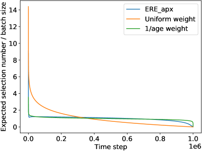
Another feature of Prop.ย 1 is an implicit 1/age weighting in Eq.ย (8). Although the original ERE samples uniformly from the recent $c_{k}$ points, the aggregate effect of all $1\leq k\leq K$ updates appears to be well approximated by a 1/age weighting. To understand the effect of 1/age, recall from sectionย 2.2 that in practice, $\hat{Q}$ is updated using mini-batch samples. Define a point (sie,aie)superscriptsubscript๐‘ ๐‘–๐‘’superscriptsubscript๐‘Ž๐‘–๐‘’(s_{i}^{e},a_{i}^{e})โ€™s time step as $i+1+L\cdot(e-1)$. Then the expected number of times in all batch samples that a point at a certain time step is selected (the expected selection number) gives the aggregate weight over the time steps. As shown in Figure.ย 1, 1/age weighting and ERE_apx, Eq.ย (8), give almost uniform expected selection numbers across time steps while uniform weighting is significantly biased toward the old samples. Therefore, 1/age weighting and its variants help balance the expected selection number.

Refer to caption
Figure 1: Expected selection numbers (aggregate weights) over a million time steps.

5.2 Merit of balanced selection number

Recall the expected selection numbers are the aggregate weights over time. To understand the merit of balanced selection numbers, we develop an error analysis under non-uniform aggregate weights in the Appendix (Theorem 2 & Corollary 2). Similar to the uniform-weight error in sectionย 4, the non-uniform-weight error is controlled by bias from policy mismatch and variance from sampling. In the following, we discuss these biases and variances in ERE, 1/age weighting, and uniform weighting. We conclude that the ERE and 1/age weighting are better because both of their biases and variances are smaller than that of uniform weighting.

For the bias from policy mismatch, Figureย 1 shows the uniform weighting (for each sampling from the replay buffer) makes the aggregate weights (expected selection number) bias toward old samples. Because the old policies tend to be distant from the current policy, the uniform weighting has a larger policy mismatch bias than ERE and 1/age weighting.

As for the variance from sampling, we generalize Corollaryย 1โ€™s uniform case: $\tilde{O}(1/\sqrt{N})$ to Corollary 2โ€™s weighted case: $\tilde{O}(\sqrt{\sum_{i}w_{i}^{2}}/\sum_{i}w_{i})$ in the Appendix. To see this, let $\{X_{i}\}_{i=1}^{N}$ be a martingale difference sequence with $0\leq X_{i}\leq\Delta$. Consider a weighted sequence $\{w_{i}X_{i}\}_{i=1}^{N}$ with weights $\{w_{i}>0\}$. The Azuma-Hoeffding inequality suggests that with probability $\geq 1-\delta$,

$\displaystyle\frac{\sum_{i}w_{i}X_{i}-\mathbb{E}[\sum_{i}w_{i}X_{i}]}{\sum_{i}w_{i}}\leq\sqrt{\frac{\sum_{i}(w_{i}\Delta)^{2}}{2}\log\frac{1}{\delta}}/\sum_{i}w_{i}=\tilde{O}\Big{(}\Delta\frac{\sqrt{\sum_{i}w_{i}^{2}}}{\sum_{i}w_{i}}\Big{)},$

which means that a general non-uniform weight admits a Hoeffding error $\tilde{O}(\sqrt{\sum_{i}w_{i}^{2}}/\sum_{i}w_{i})$ and is reduced to $\tilde{O}(1/\sqrt{N})$ when the weights are equal. Furthermore, one can prove that the Hoeffding error is minimized under uniform weights:

Proposition 2.

Let $\{w_{t}>0\}_{t=1}^{N}$ be the weights of the data indexed by $t$. Then the Hoeffding error $\sqrt{\sum_{t=1}^{N}w_{t}^{2}}/\sum_{t=1}^{N}w_{t}$ is minimized when the weights are equal: $w_{t}=c>0,~{}\forall~{}t$.

Therefore, the variance from sampling is large under non-uniform aggregate weights and is minimized by uniform aggregate weights. Since the uniform weighting leads to more non-uniform aggregate weights than ERE and 1/age weighting, its variance is also larger.

Because the ERE and 1/age weighting have balanced selection numbers (i.e., balanced aggregate weights), their biases and variance are smaller. They should perform better than uniform weighting for off-policy actor-critic RL. We will verify this in the next subsection.

5.3 Experimental verification

Since weโ€™ve established a theoretical foundation of ERE and 1/age from a bias-variance perspective, we will explore two main propositions from the preceding subsections: (1) Are ERE and 1/age weighting better than uniform weighting? (2) Does the approximated ERE proposed in Eq.ย (8) track the original ERE well? In addition, since prioritized experience replay (Schaul etย al., 2016) (PER) is a popular sampling method, a natural question to ask is (3) Do ERE and 1/age outperform PER?

We evaluate five sampling methods (ERE, ERE_apx, 1/age weighting, uniform, PER) on five MuJoCo continuous-control environments (Todorov etย al., 2012): Humanoid, Ant, Walker2d, HalfCheetah, and Hopper. All tasks have a maximum horizon of 1000 and are trained using a Pytorch Soft-Actor-Critic (Haarnoja etย al., 2018) implementation on Github (Tandon, 2018). Most hyper-parameters of the SAC algorithm are the same as that in Tandon (2018) except for the batch size, where we find a batch size of 512 tends to give more stable results. Our code is available at https://github.com/sunfex/weighted-sac. The SAC implementation and the MuJoCo environment are licensed under the MIT license and the personal student license, respectively. The experiment is run on a server with an Intel i7-6850K CPU and Nvidia GTX 1080 Ti GPUs.
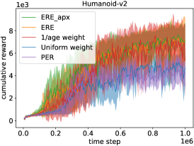
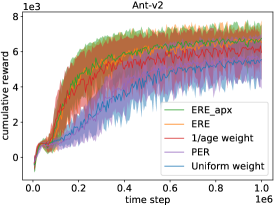
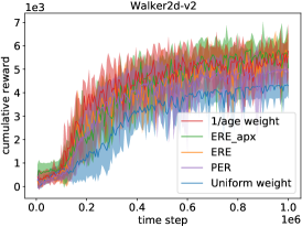
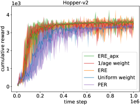
Refer to caption
Refer to caption
Refer to caption
Refer to caption
Refer to caption
Figure 2: ERE, ERE_apx, 1/age weighting and uniform weighting on MuJoCo environments in a million steps. The solid lines and shaded areas are the means and one standard deviations.

In Figureย 2, the ERE and 1/age weighting strategies perform better than the uniform weighting does in all tasks. This verifies our preceding assertion that the ERE and 1/age weighting are superior because their biases and variances of the estimated Q function are smaller. Moreover, ERE and ERE_apx mostly coincide with each other, so Eq.ย (8) is indeed a good approximation of the ERE strategy. This also explains the implicit connection between ERE and 1/age weighting strategies: ERE is almost equivalent to ERE_apx and 1/age is the main factor in ERE_apx, so ERE and 1/age weighting should produce similar results. Finally, ERE and 1/age generally outperform PER, so the 1/age-based samplings that we study achieve nontrivial performance improvements.

6 Conclusion

To understand an off-policy actor-critic algorithm, we show the policy evaluation error on the expected distribution of transitions decomposes into the Bellman error, the bias from policy mismatch, and the variance from sampling. We use this to explain that a successful off-policy actor-critic algorithm should have a careful sampling strategy that controls its bias and variance. Motivated by the empirical success of Emphasizing Recent Experience (ERE), we prove that ERE is a variant of the 1/age weighting. We then explain from a bias-variance perspective that ERE and 1/age weighting are preferable over uniform weighting because the resulting biases and variances are smaller.

References

  • Agarwal etย al. (2019) Agarwal, A., N.ย Jiang, S.ย M. Kakade, and W.ย Sun
    2019.
    Reinforcement learning: Theory and algorithms. CS Dept., UW Seattle, Seattle, WA, USA, Tech. Rep.
  • Duan etย al. (2020) Duan, Y., Z.ย Jia, and M.ย Wang
    2020.
    Minimax-optimal off-policy evaluation with linear function approximation. In Proceedings of the 37th International Conference on Machine Learning, volume 119 of Proceedings of Machine Learning Research, Pp.ย  2701โ€“2709, Virtual. PMLR.
  • Dudรญk etย al. (2011) Dudรญk, M., J.ย Langford, and L.ย Li
    2011.
    Doubly robust policy evaluation and learning. In Proceedings of the 28th International Conference on International Conference on Machine Learning, ICMLโ€™11, P.ย  1097โ€“1104, Madison, WI, USA. Omnipress.
  • Fan and Ramadge (2021) Fan, T.-H. and P.ย Ramadge
    2021.
    A contraction approach to model-based reinforcement learning. In Proceedings of The 24th International Conference on Artificial Intelligence and Statistics, A.ย Banerjee and K.ย Fukumizu, eds., volume 130 of Proceedings of Machine Learning Research, Pp.ย  325โ€“333. PMLR.
  • Feng etย al. (2020) Feng, Y., T.ย Ren, Z.ย Tang, and Q.ย Liu
    2020.
    Accountable off-policy evaluation with kernel Bellman statistics. In Proceedings of the 37th International Conference on Machine Learning, H.ย D. III and A.ย Singh, eds., volume 119 of Proceedings of Machine Learning Research, Pp.ย  3102โ€“3111. PMLR.
  • Fujimoto etย al. (2018) Fujimoto, S., H.ย van Hoof, and D.ย Meger
    2018.
    Addressing function approximation error in actor-critic methods. In Proceedings of the 35th International Conference on Machine Learning, ICML 2018, Stockholmsmรคssan, Stockholm, Sweden, July 10-15, 2018, J.ย G. Dy and A.ย Krause, eds., volumeย 80 of Proceedings of Machine Learning Research, Pp.ย  1582โ€“1591. PMLR.
  • Fujita and Maeda (2018) Fujita, Y. and S.-i. Maeda
    2018.
    Clipped action policy gradient. In Proceedings of the 35th International Conference on Machine Learning, J.ย Dy and A.ย Krause, eds., volumeย 80 of Proceedings of Machine Learning Research, Pp.ย  1597โ€“1606. PMLR.
  • Gulrajani etย al. (2017) Gulrajani, I., F.ย Ahmed, M.ย Arjovsky, V.ย Dumoulin, and A.ย C. Courville
    2017.
    Improved training of wasserstein gans. In Advances in Neural Information Processing Systems, I.ย Guyon, U.ย V. Luxburg, S.ย Bengio, H.ย Wallach, R.ย Fergus, S.ย Vishwanathan, and R.ย Garnett, eds., volumeย 30. Curran Associates, Inc.
  • Haarnoja etย al. (2018) Haarnoja, T., A.ย Zhou, P.ย Abbeel, and S.ย Levine
    2018.
    Soft actor-critic: Off-policy maximum entropy deep reinforcement learning with a stochastic actor. In Proceedings of the 35th International Conference on Machine Learning, ICML 2018, Stockholmsmรคssan, Stockholm, Sweden, July 10-15, 2018, J.ย G. Dy and A.ย Krause, eds., volumeย 80 of Proceedings of Machine Learning Research, Pp.ย  1856โ€“1865. PMLR.
  • Horgan etย al. (2018) Horgan, D., J.ย Quan, D.ย Budden, G.ย Barth-Maron, M.ย Hessel, H.ย van Hasselt, and D.ย Silver
    2018.
    Distributed prioritized experience replay. In International Conference on Learning Representations.
  • Jiang and Li (2016) Jiang, N. and L.ย Li
    2016.
    Doubly robust off-policy value evaluation for reinforcement learning. In Proceedings of The 33rd International Conference on Machine Learning, M.ย F. Balcan and K.ย Q. Weinberger, eds., volumeย 48 of Proceedings of Machine Learning Research, Pp.ย  652โ€“661, New York, New York, USA. PMLR.
  • Jin etย al. (2018) Jin, C., Z.ย Allen-Zhu, S.ย Bubeck, and M.ย I. Jordan
    2018.
    Is q-learning provably efficient? In Advances in Neural Information Processing Systems, S.ย Bengio, H.ย Wallach, H.ย Larochelle, K.ย Grauman, N.ย Cesa-Bianchi, and R.ย Garnett, eds., volumeย 31. Curran Associates, Inc.
  • Jin etย al. (2020) Jin, C., Z.ย Yang, Z.ย Wang, and M.ย I. Jordan
    2020.
    Provably efficient reinforcement learning with linear function approximation. In Conference on Learning Theory, Pp.ย  2137โ€“2143. PMLR.
  • Kallus and Uehara (2020) Kallus, N. and M.ย Uehara
    2020.
    Doubly robust off-policy value and gradient estimation for deterministic policies. In Advances in Neural Information Processing Systems, H.ย Larochelle, M.ย Ranzato, R.ย Hadsell, M.ย F. Balcan, and H.ย Lin, eds., volumeย 33, Pp.ย  10420โ€“10430. Curran Associates, Inc.
  • Lazic etย al. (2020) Lazic, N., D.ย Yin, M.ย Farajtabar, N.ย Levine, D.ย Gorur, C.ย Harris, and D.ย Schuurmans
    2020.
    A maximum-entropy approach to off-policy evaluation in average-reward mdps. Advances in Neural Information Processing Systems, 33.
  • Le etย al. (2019) Le, H., C.ย Voloshin, and Y.ย Yue
    2019.
    Batch policy learning under constraints. In International Conference on Machine Learning, Pp.ย  3703โ€“3712. PMLR.
  • Levine etย al. (2020) Levine, S., A.ย Kumar, G.ย Tucker, and J.ย Fu
    2020.
    Offline reinforcement learning: Tutorial, review, and perspectives on open problems. arXiv preprint arXiv:2005.01643.
  • Li etย al. (2020) Li, G., Y.ย Wei, Y.ย Chi, Y.ย Gu, and Y.ย Chen
    2020.
    Sample complexity of asynchronous q-learning: Sharper analysis and variance reduction. In Advances in Neural Information Processing Systems, H.ย Larochelle, M.ย Ranzato, R.ย Hadsell, M.ย F. Balcan, and H.ย Lin, eds., volumeย 33, Pp.ย  7031โ€“7043. Curran Associates, Inc.
  • Lin (1992) Lin, L.ย J.
    1992.
    Self-improving reactive agents based on reinforcement learning, planning and teaching. Machine Learning, 8:293โ€“321.
  • Liu etย al. (2018) Liu, Q., L.ย Li, Z.ย Tang, and D.ย Zhou
    2018.
    Breaking the curse of horizon: Infinite-horizon off-policy estimation. In Advances in Neural Information Processing Systems, volumeย 31, Pp.ย  5356โ€“5366. Curran Associates, Inc.
  • Luo etย al. (2019) Luo, Y., H.ย Xu, Y.ย Li, Y.ย Tian, T.ย Darrell, and T.ย Ma
    2019.
    Algorithmic framework for model-based deep reinforcement learning with theoretical guarantees. In International Conference on Learning Representations.
  • Miyato etย al. (2018) Miyato, T., T.ย Kataoka, M.ย Koyama, and Y.ย Yoshida
    2018.
    Spectral normalization for generative adversarial networks. In International Conference on Learning Representations.
  • Ni etย al. (2019) Ni, C., L.ย F. Yang, and M.ย Wang
    2019.
    Learning to control in metric space with optimal regret. In 2019 57th Annual Allerton Conference on Communication, Control, and Computing (Allerton), Pp.ย  726โ€“733.
  • Novati and Koumoutsakos (2019) Novati, G. and P.ย Koumoutsakos
    2019.
    Remember and forget for experience replay. In Proceedings of the 36th International Conference on Machine Learning, K.ย Chaudhuri and R.ย Salakhutdinov, eds., volumeย 97 of Proceedings of Machine Learning Research, Pp.ย  4851โ€“4860, Long Beach, California, USA. PMLR.
  • Precup etย al. (2000) Precup, D., R.ย S. Sutton, and S.ย P. Singh
    2000.
    Eligibility traces for off-policy policy evaluation. In Proceedings of the Seventeenth International Conference on Machine Learning, ICML โ€™00, P.ย  759โ€“766, San Francisco, CA, USA. Morgan Kaufmann Publishers Inc.
  • Schaul etย al. (2016) Schaul, T., J.ย Quan, I.ย Antonoglou, and D.ย Silver
    2016.
    Prioritized experience replay. In ICLR.
  • Schmitt etย al. (2020) Schmitt, S., M.ย Hessel, and K.ย Simonyan
    2020.
    Off-policy actor-critic with shared experience replay. In Proceedings of the 37th International Conference on Machine Learning, H.ย D. III and A.ย Singh, eds., volume 119 of Proceedings of Machine Learning Research, Pp.ย  8545โ€“8554, Virtual. PMLR.
  • Schulman etย al. (2015) Schulman, J., S.ย Levine, P.ย Abbeel, M.ย Jordan, and P.ย Moritz
    2015.
    Trust region policy optimization. In Proceedings of the 32nd International Conference on Machine Learning, F.ย Bach and D.ย Blei, eds., volumeย 37 of Proceedings of Machine Learning Research, Pp.ย  1889โ€“1897, Lille, France. PMLR.
  • Schulman etย al. (2017) Schulman, J., F.ย Wolski, P.ย Dhariwal, A.ย Radford, and O.ย Klimov
    2017.
    Proximal policy optimization algorithms. arXiv:1707.06347.
  • Silver etย al. (2014) Silver, D., G.ย Lever, N.ย Heess, T.ย Degris, D.ย Wierstra, and M.ย Riedmiller
    2014.
    Deterministic policy gradient algorithms. In Proceedings of the 31st International Conference on Machine Learning, E.ย P. Xing and T.ย Jebara, eds., volumeย 32 of Proceedings of Machine Learning Research, Pp.ย  387โ€“395, Bejing, China. PMLR.
  • Sinha etย al. (2020) Sinha, S., J.ย Song, A.ย Garg, and S.ย Ermon
    2020.
    Experience replay with likelihood-free importance weights. arXiv:2006.13169.
  • Sutton etย al. (1999) Sutton, R.ย S., D.ย McAllester, S.ย Singh, and Y.ย Mansour
    1999.
    Policy gradient methods for reinforcement learning with function approximation. In Proceedings of the 12th International Conference on Neural Information Processing Systems, NIPSโ€™99, P.ย  1057โ€“1063, Cambridge, MA, USA. MIT Press.
  • Tandon (2018) Tandon, P.
    2018.
    Pytorch soft actor critic. Github Repository,ย https://github.com/pranz24/pytorch-soft-actor-critic.
  • Thomas and Brunskill (2016) Thomas, P. and E.ย Brunskill
    2016.
    Data-efficient off-policy policy evaluation for reinforcement learning. In Proceedings of The 33rd International Conference on Machine Learning, M.ย F. Balcan and K.ย Q. Weinberger, eds., volumeย 48 of Proceedings of Machine Learning Research, Pp.ย  2139โ€“2148, New York, New York, USA. PMLR.
  • Todorov etย al. (2012) Todorov, E., T.ย Erez, and Y.ย Tassa
    2012.
    Mujoco: A physics engine for model-based control. In 2012 IEEE/RSJ International Conference on Intelligent Robots and Systems, Pp.ย  5026โ€“5033.
  • Tokdar and Kass (2010) Tokdar, S.ย T. and R.ย E. Kass
    2010.
    Importance sampling: a review. Wiley Interdisciplinary Reviews: Computational Statistics, 2(1):54โ€“60.
  • Villani (2008) Villani, C.
    2008.
    Optimal transport โ€“ Old and new, volume 338, Pp.ย  xxii+973.
  • Wang and Ross (2019) Wang, C. and K.ย Ross
    2019.
    Boosting soft actor-critic: Emphasizing recent experience without forgetting the past. arXiv:1906.04009.
  • Xiao etย al. (2019) Xiao, C., Y.ย Wu, C.ย Ma, D.ย Schuurmans, and M.ย Mรผller
    2019.
    Learning to combat compounding-error in model-based reinforcement learning. arXiv:1912.11206.
  • Xie etย al. (2019) Xie, T., Y.ย Ma, and Y.-X. Wang
    2019.
    Towards optimal off-policy evaluation for reinforcement learning with marginalized importance sampling. In Advances in Neural Information Processing Systems, volumeย 32, Pp.ย  9668โ€“9678. Curran Associates, Inc.
  • Yang etย al. (2020) Yang, M., O.ย Nachum, B.ย Dai, L.ย Li, and D.ย Schuurmans
    2020.
    Off-policy evaluation via the regularized lagrangian. Advances in Neural Information Processing Systems, 33.
  • Yin etย al. (2021) Yin, M., Y.ย Bai, and Y.-X. Wang
    2021.
    Near-optimal provable uniform convergence in offline policy evaluation for reinforcement learning. In Proceedings of The 24th International Conference on Artificial Intelligence and Statistics, A.ย Banerjee and K.ย Fukumizu, eds., volume 130 of Proceedings of Machine Learning Research, Pp.ย  1567โ€“1575. PMLR.
  • Yin and Wang (2020) Yin, M. and Y.-X. Wang
    2020.
    Asymptotically efficient off-policy evaluation for tabular reinforcement learning. In Proceedings of the Twenty Third International Conference on Artificial Intelligence and Statistics, S.ย Chiappa and R.ย Calandra, eds., volume 108 of Proceedings of Machine Learning Research, Pp.ย  3948โ€“3958, Online. PMLR.
  • Yu etย al. (2020) Yu, T., G.ย Thomas, L.ย Yu, S.ย Ermon, J.ย Y. Zou, S.ย Levine, C.ย Finn, and T.ย Ma
    2020.
    Mopo: Model-based offline policy optimization. In Advances in Neural Information Processing Systems, H.ย Larochelle, M.ย Ranzato, R.ย Hadsell, M.ย F. Balcan, and H.ย Lin, eds., volumeย 33, Pp.ย  14129โ€“14142. Curran Associates, Inc.

Appendix A Appendix

A.1 Hyper-parameters

To train the SAC agents, we use deep neural networks to parameterize the policy and Q functions. Both networks consist of dense layers with the same widths. Tableย 1 presents the suggested hyper-parameters. As mentioned in the experiment section, the hyper-parameters are similar as the implementation in Tandon (2018).

Variable Value
Optimizer Adam
Learning rate 3E-4
Discount factor 0.99
Batch size 512
Model width 256
Model depth 3
Table 1: Suggested hyper-parameters for SAC.
Environment Hopper HalfCheetah Walker2D Ant Humanoid
Temperature 0.2 0.2 0.2 0.2 0.05
Table 2: Temperature parameters for SAC in MuJoCo environments.

A.2 Justification of assumptions

In sectionย 4.1, we introduce three main assumptions in this work. Below is a validation for each.

  • 1.

    For each sโˆˆ๐’ฎ,๐‘ ๐’ฎs\in\mathcal{S}, Q^โ€‹(s,a)bold-^๐‘„๐‘ ๐‘Ž\hat{Q}(s,a) and Qฯ€Nโ€‹(s,a)superscript๐‘„superscript๐œ‹๐‘๐‘ ๐‘ŽQ^{\pi^{N}}(s,a) are $L_{\mathcal{A}}$-Lipschitz in $a.$ As mentioned in the paragraph โ€Normalizationโ€ of sectionย 4.2, the Lipschitzness of $Q^{\pi^{N}}$ is sublinear or linear in the horizon, which quantifies the magnitude of $Q^{\pi^{N}}$โ€™s Lipschitz constant. Since $\hat{Q}$ approximates $Q^{\pi^{N}}$, $\hat{Q}$ should have a similar property as long as the training error is well controlled. The practitioner can also enforce the Lipschitzness of $\hat{Q}$ using gradient penalty (Gulrajani etย al., 2017) or spectral normalization (Miyato etย al., 2018).

  • 2.

    $\hat{Q}(s,a)$ and Qฯ€Nโ€‹(s,a)superscript๐‘„superscript๐œ‹๐‘๐‘ ๐‘ŽQ^{\pi^{N}}(s,a) are bounded and take values in $[0,r^{\max}/(1-\gamma)]$. This is a standard assumption in the RL literature. If the bound is violated, one can either clip, translate, or rescale to obtain new Q functions that satisfy the constraint. Note a bounded reward rโ€‹(s,a)โˆˆ[0,rmax]๐‘Ÿ๐‘ ๐‘Ž0superscript๐‘Ÿr(s,a)\in[0,r^{\max}] has implied $Q^{\pi^{N}}\in[0,r^{\max}/(1-\gamma)]$.

  • 3.

    The action space is bounded with diameter $\text{diam}_{\mathcal{A}}<\infty$. This is a standard assumption in continuous-control environments and is usually satisfied in practice. It is also common to use clipping to ensure the bounds of the actions generated by the policy (Fujita and Maeda, 2018).

A.3 The construction of our behavior policy

We first discuss some important relations between state occupancy measures and Bellman flow operator. Similar results about Factย 1 and 2 be found in Liu etย al. (2018)[Lemma 3] and Fan and Ramadge (2021)[Appendix A.1].

Definition 1 (Bellman flow operator).

The Bellman flow operator $B_{\rho_{0},\pi,T}(\cdot)$ generated by $(\rho_{0},\pi,T)$ with discount factor $\gamma$ is defined as

Bฯ0,ฯ€,Tโ€‹(ฯ)โ€‹(s)โ‰œ(1โˆ’ฮณ)โ€‹ฯ0โ€‹(s)+ฮณโ€‹โˆซTโ€‹(s|sโ€ฒ,aโ€ฒ)โ€‹ฯ€โ€‹(aโ€ฒ|sโ€ฒ)โ€‹ฯโ€‹(sโ€ฒ)โ€‹๐‘‘sโ€ฒโ€‹๐‘‘aโ€ฒ.โ‰œsubscript๐ตsubscript๐œŒ0๐œ‹๐‘‡๐œŒ๐‘ 1๐›พsubscript๐œŒ0๐‘ ๐›พ๐‘‡conditional๐‘ superscript๐‘ โ€ฒsuperscript๐‘Žโ€ฒ๐œ‹conditionalsuperscript๐‘Žโ€ฒsuperscript๐‘ โ€ฒ๐œŒsuperscript๐‘ โ€ฒdifferential-dsuperscript๐‘ โ€ฒdifferential-dsuperscript๐‘Žโ€ฒB_{\rho_{0},\pi,T}(\rho)(s)\triangleq(1-\gamma)\rho_{0}(s)+\gamma\int T(s|s^{\prime},a^{\prime})\pi(a^{\prime}|s^{\prime})\rho(s^{\prime})ds^{\prime}da^{\prime}.
Fact 1.

$B_{\rho_{0},\pi,T}$ is a $\gamma$-contraction w.r.t. total variational distance.

Proof.

Let p1โ€‹(s),p2โ€‹(s)subscript๐‘1๐‘ subscript๐‘2๐‘ p_{1}(s),~{}p_{2}(s) be the density functions of some state distributions.

DTโ€‹Vโ€‹(Bฯ0,ฯ€,Tโ€‹(p1)โ€‹||โ€‹Bฯ0,ฯ€,Tโ€‹(p2))=12โ€‹โˆซ|Bฯ0,ฯ€,Tโ€‹(p1โ€‹(s))โˆ’Bฯ0,ฯ€,Tโ€‹(p2โ€‹(s))|โ€‹๐‘‘s=12โ€‹โˆซฮณโ€‹|โˆซTโ€‹(s|sโ€ฒ,aโ€ฒ)โ€‹ฯ€โ€‹(aโ€ฒ|sโ€ฒ)โ€‹(p1โ€‹(sโ€ฒ)โˆ’p2โ€‹(sโ€ฒ))โ€‹๐‘‘sโ€ฒโ€‹๐‘‘aโ€ฒ|โ€‹๐‘‘sโ‰คฮณ2โ€‹โˆซTโ€‹(s|sโ€ฒ,aโ€ฒ)โ€‹ฯ€โ€‹(aโ€ฒ|sโ€ฒ)โ€‹|p1โ€‹(sโ€ฒ)โˆ’p2โ€‹(sโ€ฒ)|โ€‹๐‘‘sโ€ฒโ€‹๐‘‘aโ€ฒโ€‹๐‘‘s=ฮณ2โ€‹โˆซ|p1โ€‹(sโ€ฒ)โˆ’p2โ€‹(sโ€ฒ)|โ€‹๐‘‘sโ€ฒ=ฮณโ€‹DTโ€‹Vโ€‹(p1โ€‹||โ€‹p2).subscript๐ท๐‘‡๐‘‰subscript๐ตsubscript๐œŒ0๐œ‹๐‘‡subscript๐‘1subscript๐ตsubscript๐œŒ0๐œ‹๐‘‡subscript๐‘212subscript๐ตsubscript๐œŒ0๐œ‹๐‘‡subscript๐‘1๐‘ subscript๐ตsubscript๐œŒ0๐œ‹๐‘‡subscript๐‘2๐‘ differential-d๐‘ 12๐›พ๐‘‡conditional๐‘ superscript๐‘ โ€ฒsuperscript๐‘Žโ€ฒ๐œ‹conditionalsuperscript๐‘Žโ€ฒsuperscript๐‘ โ€ฒsubscript๐‘1superscript๐‘ โ€ฒsubscript๐‘2superscript๐‘ โ€ฒdifferential-dsuperscript๐‘ โ€ฒdifferential-dsuperscript๐‘Žโ€ฒdifferential-d๐‘ ๐›พ2๐‘‡conditional๐‘ superscript๐‘ โ€ฒsuperscript๐‘Žโ€ฒ๐œ‹conditionalsuperscript๐‘Žโ€ฒsuperscript๐‘ โ€ฒsubscript๐‘1superscript๐‘ โ€ฒsubscript๐‘2superscript๐‘ โ€ฒdifferential-dsuperscript๐‘ โ€ฒdifferential-dsuperscript๐‘Žโ€ฒdifferential-d๐‘ ๐›พ2subscript๐‘1superscript๐‘ โ€ฒsubscript๐‘2superscript๐‘ โ€ฒdifferential-dsuperscript๐‘ โ€ฒ๐›พsubscript๐ท๐‘‡๐‘‰subscript๐‘1subscript๐‘2\begin{split}D_{TV}(B_{\rho_{0},\pi,T}(p_{1})\lvert\rvert B_{\rho_{0},\pi,T}(p_{2}))&=\frac{1}{2}\int\big{\lvert}B_{\rho_{0},\pi,T}(p_{1}(s))-B_{\rho_{0},\pi,T}(p_{2}(s))\big{\rvert}ds\\ &=\frac{1}{2}\int\gamma\Big{\lvert}\int T(s|s^{\prime},a^{\prime})\pi(a^{\prime}|s^{\prime})\big{(}p_{1}(s^{\prime})-p_{2}(s^{\prime})\big{)}ds^{\prime}da^{\prime}\Big{\rvert}ds\\ &\leq\frac{\gamma}{2}\int T(s|s^{\prime},a^{\prime})\pi(a^{\prime}|s^{\prime})\big{\lvert}p_{1}(s^{\prime})-p_{2}(s^{\prime})\big{\rvert}ds^{\prime}da^{\prime}ds\\ &=\frac{\gamma}{2}\int\big{\lvert}p_{1}(s^{\prime})-p_{2}(s^{\prime})\big{\rvert}ds^{\prime}=\gamma D_{TV}(p_{1}\lvert\rvert p_{2}).\end{split}

โˆŽ

Fact 2.

The normalized state occupancy measure $\rho_{\rho_{0}}^{\pi}$ generated by $(\rho_{0},\pi,T)$ with discount factor $\gamma$ is a fixed point of $B_{\rho_{0},\pi,T}$; i.e., Bฯ0,ฯ€,Tโ€‹(ฯฯ0ฯ€)โ€‹(s)=ฯฯ0ฯ€โ€‹(s)subscript๐ตsubscript๐œŒ0๐œ‹๐‘‡superscriptsubscript๐œŒsubscript๐œŒ0๐œ‹๐‘ superscriptsubscript๐œŒsubscript๐œŒ0๐œ‹๐‘ B_{\rho_{0},\pi,T}(\rho_{\rho_{0}}^{\pi})(s)=\rho_{\rho_{0}}^{\pi}(s).

Proof.
ฯฯ0ฯ€โ€‹(s)=(1โˆ’ฮณ)โ€‹โˆ‘i=0โˆžฮณiโ€‹fiโ€‹(s|ฯ0,ฯ€,T)=(1โˆ’ฮณ)โ€‹f0โ€‹(s|ฯ0,ฯ€,T)+ฮณโ€‹(1โˆ’ฮณ)โ€‹โˆ‘i=0โˆžฮณiโ€‹fi+1โ€‹(s|ฯ0,ฯ€,T)=(1โˆ’ฮณ)โ€‹ฯ0โ€‹(s)+ฮณโ€‹(1โˆ’ฮณ)โ€‹โˆ‘i=0โˆžฮณiโ€‹โˆซTโ€‹(s|sโ€ฒ,aโ€ฒ)โ€‹ฯ€โ€‹(aโ€ฒ|sโ€ฒ)โ€‹fiโ€‹(sโ€ฒ|ฯ0,ฯ€,T)โ€‹๐‘‘sโ€ฒโ€‹๐‘‘aโ€ฒ=(1โˆ’ฮณ)โ€‹ฯ0โ€‹(s)+ฮณโ€‹โˆซTโ€‹(s|sโ€ฒ,aโ€ฒ)โ€‹ฯ€โ€‹(aโ€ฒ|sโ€ฒ)โ€‹(1โˆ’ฮณ)โ€‹โˆ‘i=0โˆžฮณiโ€‹fiโ€‹(sโ€ฒ|ฯ0,ฯ€,T)โ€‹dโ€‹sโ€ฒโ€‹dโ€‹aโ€ฒ=(1โˆ’ฮณ)โ€‹ฯ0โ€‹(s)+ฮณโ€‹โˆซTโ€‹(s|sโ€ฒ,aโ€ฒ)โ€‹ฯ€โ€‹(aโ€ฒ|sโ€ฒ)โ€‹ฯฯ0ฯ€โ€‹(sโ€ฒ)โ€‹๐‘‘sโ€ฒโ€‹๐‘‘aโ€ฒ=Bฯ0,ฯ€,Tโ€‹(ฯฯ0ฯ€)โ€‹(s).superscriptsubscript๐œŒsubscript๐œŒ0๐œ‹๐‘ 1๐›พsuperscriptsubscript๐‘–0superscript๐›พ๐‘–subscript๐‘“๐‘–conditional๐‘ subscript๐œŒ0๐œ‹๐‘‡1๐›พsubscript๐‘“0conditional๐‘ subscript๐œŒ0๐œ‹๐‘‡๐›พ1๐›พsuperscriptsubscript๐‘–0superscript๐›พ๐‘–subscript๐‘“๐‘–1conditional๐‘ subscript๐œŒ0๐œ‹๐‘‡1๐›พsubscript๐œŒ0๐‘ ๐›พ1๐›พsuperscriptsubscript๐‘–0superscript๐›พ๐‘–๐‘‡conditional๐‘ superscript๐‘ โ€ฒsuperscript๐‘Žโ€ฒ๐œ‹conditionalsuperscript๐‘Žโ€ฒsuperscript๐‘ โ€ฒsubscript๐‘“๐‘–conditionalsuperscript๐‘ โ€ฒsubscript๐œŒ0๐œ‹๐‘‡differential-dsuperscript๐‘ โ€ฒdifferential-dsuperscript๐‘Žโ€ฒ1๐›พsubscript๐œŒ0๐‘ ๐›พ๐‘‡conditional๐‘ superscript๐‘ โ€ฒsuperscript๐‘Žโ€ฒ๐œ‹conditionalsuperscript๐‘Žโ€ฒsuperscript๐‘ โ€ฒ1๐›พsuperscriptsubscript๐‘–0superscript๐›พ๐‘–subscript๐‘“๐‘–conditionalsuperscript๐‘ โ€ฒsubscript๐œŒ0๐œ‹๐‘‡๐‘‘superscript๐‘ โ€ฒ๐‘‘superscript๐‘Žโ€ฒ1๐›พsubscript๐œŒ0๐‘ ๐›พ๐‘‡conditional๐‘ superscript๐‘ โ€ฒsuperscript๐‘Žโ€ฒ๐œ‹conditionalsuperscript๐‘Žโ€ฒsuperscript๐‘ โ€ฒsuperscriptsubscript๐œŒsubscript๐œŒ0๐œ‹superscript๐‘ โ€ฒdifferential-dsuperscript๐‘ โ€ฒdifferential-dsuperscript๐‘Žโ€ฒsubscript๐ตsubscript๐œŒ0๐œ‹๐‘‡superscriptsubscript๐œŒsubscript๐œŒ0๐œ‹๐‘ \begin{split}\rho_{\rho_{0}}^{\pi}(s)=&(1-\gamma)\sum_{i=0}^{\infty}\gamma^{i}f_{i}(s|\rho_{0},\pi,T)\\ =&(1-\gamma)f_{0}(s|\rho_{0},\pi,T)+\gamma(1-\gamma)\sum_{i=0}^{\infty}\gamma^{i}f_{i+1}(s|\rho_{0},\pi,T)\\ =&(1-\gamma)\rho_{0}(s)+\gamma(1-\gamma)\sum_{i=0}^{\infty}\gamma^{i}\int T(s|s^{\prime},a^{\prime})\pi(a^{\prime}|s^{\prime})f_{i}(s^{\prime}|\rho_{0},\pi,T)ds^{\prime}da^{\prime}\\ =&(1-\gamma)\rho_{0}(s)+\gamma\int T(s|s^{\prime},a^{\prime})\pi(a^{\prime}|s^{\prime})(1-\gamma)\sum_{i=0}^{\infty}\gamma^{i}f_{i}(s^{\prime}|\rho_{0},\pi,T)ds^{\prime}da^{\prime}\\ =&(1-\gamma)\rho_{0}(s)+\gamma\int T(s|s^{\prime},a^{\prime})\pi(a^{\prime}|s^{\prime})\rho_{\rho_{0}}^{\pi}(s^{\prime})ds^{\prime}da^{\prime}=B_{\rho_{0},\pi,T}(\rho_{\rho_{0}}^{\pi})(s).\end{split}

โˆŽ

Thus, the Bellman flow operator is useful to analyze the state occupancy measures, and we have the following lemma to construct the behavior policy $\pi_{i}^{D}$.

Lemma 1.

Let ฯieโ€‹(s)superscriptsubscript๐œŒ๐‘–๐‘’๐‘ \rho_{i}^{e}(s) the state distribution at trajectory step $i$ in episode $e$. Let ฯฯieฯ€eโ€‹(s)superscriptsubscript๐œŒsuperscriptsubscript๐œŒ๐‘–๐‘’superscript๐œ‹๐‘’๐‘ \rho_{\rho_{i}^{e}}^{\pi^{e}}(s) be the normalized occupancy measure starting at trajectory step $i$ in episode $e$. Then 1Nโ€‹โˆ‘e=1Nฯฯieฯ€eโ€‹(s)=ฯฯยฏiฯ€iDโ€‹(s)โ€‹a.e.formulae-sequence1๐‘superscriptsubscript๐‘’1๐‘superscriptsubscript๐œŒsuperscriptsubscript๐œŒ๐‘–๐‘’superscript๐œ‹๐‘’๐‘ superscriptsubscript๐œŒsubscriptยฏ๐œŒ๐‘–superscriptsubscript๐œ‹๐‘–๐ท๐‘ ๐‘Ž๐‘’\frac{1}{N}\sum_{e=1}^{N}\rho_{\rho_{i}^{e}}^{\pi^{e}}(s)=\rho_{\overline{\rho}_{i}}^{\pi_{i}^{D}}(s)~{}a.e., where $\rho_{\overline{\rho}_{i}}^{\pi_{i}^{D}}$ is the normalized state occupancy measure is generated by $(\overline{\rho}_{i},\pi_{i}^{D},T)$. Moreover, we have 1Nโ€‹โˆ‘e=1Nฯฯieฯ€eโ€‹(s)โ€‹ฯ€eโ€‹(a|s)=ฯฯยฏiฯ€iDโ€‹(s)โ€‹ฯ€iDโ€‹(a|s)โ€‹a.e.formulae-sequence1๐‘superscriptsubscript๐‘’1๐‘superscriptsubscript๐œŒsuperscriptsubscript๐œŒ๐‘–๐‘’superscript๐œ‹๐‘’๐‘ superscript๐œ‹๐‘’conditional๐‘Ž๐‘ superscriptsubscript๐œŒsubscriptยฏ๐œŒ๐‘–superscriptsubscript๐œ‹๐‘–๐ท๐‘ subscriptsuperscript๐œ‹๐ท๐‘–conditional๐‘Ž๐‘ ๐‘Ž๐‘’\frac{1}{N}\sum_{e=1}^{N}\rho_{\rho_{i}^{e}}^{\pi^{e}}(s)\pi^{e}(a|s)=\rho_{\overline{\rho}_{i}}^{\pi_{i}^{D}}(s)\pi^{D}_{i}(a|s)~{}a.e.

Proof.

Precisely, ฯieโ€‹(s)=ฯiโ€‹(s|ฯ0,ฯ€e,T)superscriptsubscript๐œŒ๐‘–๐‘’๐‘ subscript๐œŒ๐‘–conditional๐‘ subscript๐œŒ0superscript๐œ‹๐‘’๐‘‡\rho_{i}^{e}(s)=\rho_{i}(s|\rho_{0},\pi^{e},T) is the state distribution at trajectory step $i$ following the laws of $(\rho_{0},\pi^{e},T)$. Since $\rho_{\rho_{i}^{e}}^{\pi^{e}}$ is the normalized occupancy measure generated by $(\rho_{i}^{e},\pi^{e},T)$, each $\rho_{\rho_{i}^{e}}^{\pi^{e}}$ is the fixed-point of the Bellman flow equation:

ฯฯieฯ€eโ€‹(s)=(1โˆ’ฮณ)โ€‹ฯieโ€‹(s)+ฮณโ€‹โˆซTโ€‹(s|sโ€ฒ,aโ€ฒ)โ€‹ฯ€eโ€‹(aโ€ฒ|sโ€ฒ)โ€‹ฯฯieฯ€eโ€‹(sโ€ฒ)โ€‹๐‘‘sโ€ฒโ€‹๐‘‘aโ€ฒ,โˆ€eโˆˆ[1,โ€ฆ,N].formulae-sequencesuperscriptsubscript๐œŒsuperscriptsubscript๐œŒ๐‘–๐‘’superscript๐œ‹๐‘’๐‘ 1๐›พsuperscriptsubscript๐œŒ๐‘–๐‘’๐‘ ๐›พ๐‘‡conditional๐‘ superscript๐‘ โ€ฒsuperscript๐‘Žโ€ฒsuperscript๐œ‹๐‘’conditionalsuperscript๐‘Žโ€ฒsuperscript๐‘ โ€ฒsuperscriptsubscript๐œŒsuperscriptsubscript๐œŒ๐‘–๐‘’superscript๐œ‹๐‘’superscript๐‘ โ€ฒdifferential-dsuperscript๐‘ โ€ฒdifferential-dsuperscript๐‘Žโ€ฒfor-all๐‘’1โ€ฆ๐‘\rho_{\rho_{i}^{e}}^{\pi^{e}}(s)=(1-\gamma)\rho_{i}^{e}(s)+\gamma\int T(s|s^{\prime},a^{\prime})\pi^{e}(a^{\prime}|s^{\prime})\rho_{\rho_{i}^{e}}^{\pi^{e}}(s^{\prime})ds^{\prime}da^{\prime},~{}~{}~{}\forall~{}e\in[1,...,N].

This implies the average normalized occupancy measure is the fixed point of the Bellman flow equation characterized by $(\overline{\rho}_{i},\pi_{i}^{D},T)$:

1Nโ€‹โˆ‘e=1Nฯฯieฯ€eโ€‹(s)1๐‘superscriptsubscript๐‘’1๐‘superscriptsubscript๐œŒsuperscriptsubscript๐œŒ๐‘–๐‘’superscript๐œ‹๐‘’๐‘ \displaystyle\frac{1}{N}\sum_{e=1}^{N}\rho_{\rho_{i}^{e}}^{\pi^{e}}(s) =1Nโ€‹โˆ‘e=1N[(1โˆ’ฮณ)โ€‹ฯieโ€‹(s)+ฮณโ€‹โˆซTโ€‹(s|sโ€ฒ,aโ€ฒ)โ€‹ฯ€eโ€‹(aโ€ฒ|sโ€ฒ)โ€‹ฯฯieฯ€eโ€‹(sโ€ฒ)โ€‹๐‘‘sโ€ฒโ€‹๐‘‘aโ€ฒ]absent1๐‘superscriptsubscript๐‘’1๐‘delimited-[]1๐›พsuperscriptsubscript๐œŒ๐‘–๐‘’๐‘ ๐›พ๐‘‡conditional๐‘ superscript๐‘ โ€ฒsuperscript๐‘Žโ€ฒsuperscript๐œ‹๐‘’conditionalsuperscript๐‘Žโ€ฒsuperscript๐‘ โ€ฒsuperscriptsubscript๐œŒsuperscriptsubscript๐œŒ๐‘–๐‘’superscript๐œ‹๐‘’superscript๐‘ โ€ฒdifferential-dsuperscript๐‘ โ€ฒdifferential-dsuperscript๐‘Žโ€ฒ\displaystyle=\frac{1}{N}\sum_{e=1}^{N}\left[(1-\gamma)\rho_{i}^{e}(s)+\gamma\int T(s|s^{\prime},a^{\prime})\pi^{e}(a^{\prime}|s^{\prime})\rho_{\rho_{i}^{e}}^{\pi^{e}}(s^{\prime})ds^{\prime}da^{\prime}\right]
=(1โˆ’ฮณ)โ€‹ฯยฏiโ€‹(s)+ฮณโ€‹โˆซTโ€‹(s|sโ€ฒ,aโ€ฒ)โ€‹1Nโ€‹โˆ‘e=1N[ฯ€eโ€‹(aโ€ฒ|sโ€ฒ)โ€‹ฯฯieฯ€eโ€‹(sโ€ฒ)]โ€‹dโ€‹sโ€ฒโ€‹dโ€‹aโ€ฒabsent1๐›พsubscriptยฏ๐œŒ๐‘–๐‘ ๐›พ๐‘‡conditional๐‘ superscript๐‘ โ€ฒsuperscript๐‘Žโ€ฒ1๐‘superscriptsubscript๐‘’1๐‘delimited-[]superscript๐œ‹๐‘’conditionalsuperscript๐‘Žโ€ฒsuperscript๐‘ โ€ฒsuperscriptsubscript๐œŒsuperscriptsubscript๐œŒ๐‘–๐‘’superscript๐œ‹๐‘’superscript๐‘ โ€ฒ๐‘‘superscript๐‘ โ€ฒ๐‘‘superscript๐‘Žโ€ฒ\displaystyle=(1-\gamma)\overline{\rho}_{i}(s)+\gamma\int T(s|s^{\prime},a^{\prime})\frac{1}{N}\sum_{e=1}^{N}\left[\pi^{e}(a^{\prime}|s^{\prime})\rho_{\rho_{i}^{e}}^{\pi^{e}}(s^{\prime})\right]ds^{\prime}da^{\prime}
=(1โˆ’ฮณ)โ€‹ฯยฏiโ€‹(s)+ฮณโ€‹โˆซTโ€‹(s|sโ€ฒ,aโ€ฒ)โ€‹โˆ‘e=1Nฯ€eโ€‹(aโ€ฒ|sโ€ฒ)โ€‹ฯฯieฯ€eโ€‹(sโ€ฒ)โˆ‘e=1Nฯฯieฯ€eโ€‹(sโ€ฒ)โ€‹โˆ‘e=1Nฯฯieฯ€eโ€‹(sโ€ฒ)Nโ€‹๐‘‘sโ€ฒโ€‹๐‘‘aโ€ฒabsent1๐›พsubscriptยฏ๐œŒ๐‘–๐‘ ๐›พ๐‘‡conditional๐‘ superscript๐‘ โ€ฒsuperscript๐‘Žโ€ฒsuperscriptsubscript๐‘’1๐‘superscript๐œ‹๐‘’conditionalsuperscript๐‘Žโ€ฒsuperscript๐‘ โ€ฒsuperscriptsubscript๐œŒsuperscriptsubscript๐œŒ๐‘–๐‘’superscript๐œ‹๐‘’superscript๐‘ โ€ฒsuperscriptsubscript๐‘’1๐‘superscriptsubscript๐œŒsuperscriptsubscript๐œŒ๐‘–๐‘’superscript๐œ‹๐‘’superscript๐‘ โ€ฒsuperscriptsubscript๐‘’1๐‘superscriptsubscript๐œŒsuperscriptsubscript๐œŒ๐‘–๐‘’superscript๐œ‹๐‘’superscript๐‘ โ€ฒ๐‘differential-dsuperscript๐‘ โ€ฒdifferential-dsuperscript๐‘Žโ€ฒ\displaystyle=(1-\gamma)\overline{\rho}_{i}(s)+\gamma\int T(s|s^{\prime},a^{\prime})\frac{\sum_{e=1}^{N}\pi^{e}(a^{\prime}|s^{\prime})\rho_{\rho_{i}^{e}}^{\pi^{e}}(s^{\prime})}{\sum_{e=1}^{N}\rho_{\rho_{i}^{e}}^{\pi^{e}}(s^{\prime})}\frac{\sum_{e=1}^{N}\rho_{\rho_{i}^{e}}^{\pi^{e}}(s^{\prime})}{N}ds^{\prime}da^{\prime}
=(1โˆ’ฮณ)โ€‹ฯยฏiโ€‹(s)+ฮณโ€‹โˆซTโ€‹(s|sโ€ฒ,aโ€ฒ)โ€‹ฯ€iDโ€‹(aโ€ฒ|sโ€ฒ)โ€‹1Nโ€‹โˆ‘e=1Nฯฯieฯ€eโ€‹(sโ€ฒ)โ€‹dโ€‹sโ€ฒโ€‹dโ€‹aโ€ฒ,absent1๐›พsubscriptยฏ๐œŒ๐‘–๐‘ ๐›พ๐‘‡conditional๐‘ superscript๐‘ โ€ฒsuperscript๐‘Žโ€ฒsuperscriptsubscript๐œ‹๐‘–๐ทconditionalsuperscript๐‘Žโ€ฒsuperscript๐‘ โ€ฒ1๐‘superscriptsubscript๐‘’1๐‘superscriptsubscript๐œŒsuperscriptsubscript๐œŒ๐‘–๐‘’superscript๐œ‹๐‘’superscript๐‘ โ€ฒ๐‘‘superscript๐‘ โ€ฒ๐‘‘superscript๐‘Žโ€ฒ\displaystyle=(1-\gamma)\overline{\rho}_{i}(s)+\gamma\int T(s|s^{\prime},a^{\prime})\pi_{i}^{D}(a^{\prime}|s^{\prime})\frac{1}{N}\sum_{e=1}^{N}\rho_{\rho_{i}^{e}}^{\pi^{e}}(s^{\prime})ds^{\prime}da^{\prime},

where ฯ€iDโ€‹(a|s)โ‰œโˆ‘e=1Nฯ€eโ€‹(a|s)โ€‹ฯฯieฯ€eโ€‹(s)โˆ‘e=1Nฯฯieฯ€eโ€‹(s)โ‰œsuperscriptsubscript๐œ‹๐‘–๐ทconditional๐‘Ž๐‘ superscriptsubscript๐‘’1๐‘superscript๐œ‹๐‘’conditional๐‘Ž๐‘ superscriptsubscript๐œŒsuperscriptsubscript๐œŒ๐‘–๐‘’superscript๐œ‹๐‘’๐‘ superscriptsubscript๐‘’1๐‘superscriptsubscript๐œŒsuperscriptsubscript๐œŒ๐‘–๐‘’superscript๐œ‹๐‘’๐‘ \pi_{i}^{D}(a|s)\triangleq\frac{\sum_{e=1}^{N}\pi^{e}(a|s)\rho_{\rho_{i}^{e}}^{\pi^{e}}(s)}{\sum_{e=1}^{N}\rho_{\rho_{i}^{e}}^{\pi^{e}}(s)} is the average behavior policy at step $i$. Since the Bellman flow operator is a $\gamma$-contraction in TV distance and hence has a unique fixed point in TV distance, denoted as ฯฯยฏiฯ€iDโ€‹(s)superscriptsubscript๐œŒsubscriptยฏ๐œŒ๐‘–superscriptsubscript๐œ‹๐‘–๐ท๐‘ \rho_{\overline{\rho}_{i}}^{\pi_{i}^{D}}(s), we arrive at 1Nโ€‹โˆ‘e=1Nฯฯieฯ€eโ€‹(s)=ฯฯยฏiฯ€iDโ€‹(s)1๐‘superscriptsubscript๐‘’1๐‘superscriptsubscript๐œŒsuperscriptsubscript๐œŒ๐‘–๐‘’superscript๐œ‹๐‘’๐‘ superscriptsubscript๐œŒsubscriptยฏ๐œŒ๐‘–superscriptsubscript๐œ‹๐‘–๐ท๐‘ \frac{1}{N}\sum_{e=1}^{N}\rho_{\rho_{i}^{e}}^{\pi^{e}}(s)=\rho_{\overline{\rho}_{i}}^{\pi_{i}^{D}}(s) almost everywhere. Also, by construction, we have

1Nโ€‹โˆ‘e=1Nฯฯieฯ€eโ€‹(s)โ€‹ฯ€eโ€‹(a|s)=ฯฯยฏiฯ€iDโ€‹(s)โ€‹ฯ€iDโ€‹(a|s)โ€‹a.e.formulae-sequence1๐‘superscriptsubscript๐‘’1๐‘superscriptsubscript๐œŒsuperscriptsubscript๐œŒ๐‘–๐‘’superscript๐œ‹๐‘’๐‘ superscript๐œ‹๐‘’conditional๐‘Ž๐‘ superscriptsubscript๐œŒsubscriptยฏ๐œŒ๐‘–superscriptsubscript๐œ‹๐‘–๐ท๐‘ subscriptsuperscript๐œ‹๐ท๐‘–conditional๐‘Ž๐‘ ๐‘Ž๐‘’\frac{1}{N}\sum_{e=1}^{N}\rho_{\rho_{i}^{e}}^{\pi^{e}}(s)\pi^{e}(a|s)=\rho_{\overline{\rho}_{i}}^{\pi_{i}^{D}}(s)\pi^{D}_{i}(a|s)~{}a.e.

โˆŽ

A.4 Policy Evaluation Error

Lemma 2.

If Qโ€‹(s,a)๐‘„๐‘ ๐‘ŽQ(s,a) is $L_{\mathcal{A}}$-Lipschitz in $a$ for any s๐‘ s, then, for any state distribution $\rho$,

$$\mathbb{E}_{s\sim\rho}\Big{|}\mathbb{E}_{a\sim\pi_{1}(\cdot|s)}Q(s,a)-\mathbb{E}_{a\sim\pi_{2}(\cdot|s)}Q(s,a)\Big{|}\leq L_{\mathcal{A}}\mathbb{E}_{s\sim\rho}W_{1}(\pi_{1}(\cdot|s)\lvert\rvert\pi_{2}(\cdot|s)).$$
Proof.

For any fixed s๐‘ s, we have

$\displaystyle\mathbb{E}_{a\sim\pi_{1}(\cdot|s)}Q(s,a)-\mathbb{E}_{a\sim\pi_{2}(\cdot|s)}Q(s,a)=L_{\mathcal{A}}\Big{[}\mathbb{E}_{a\sim\pi_{1}(\cdot|s)}\frac{Q(s,a)}{L_{\mathcal{A}}}-\mathbb{E}_{a\sim\pi_{2}(\cdot|s)}\frac{Q(s,a)}{L_{\mathcal{A}}}\Big{]}$
$\displaystyle\leq$ $\displaystyle L_{\mathcal{A}}\Big{[}\sup_{\|f\|_{\text{Lip}}\leq 1}\mathbb{E}_{a\sim\pi_{1}(\cdot|s)}f(a)-\mathbb{E}_{a\sim\pi_{2}(\cdot|s)}f(a)\Big{]}=L_{\mathcal{A}}W_{1}(\pi_{1}(\cdot|s)\lvert\rvert\pi_{2}(\cdot|s)),$

where the second line follows from Kantorovich-Rubinstein duality (Villani, 2008). Since the 1-Wasserstein distance $W_{1}$ is symmetric, we can interchange the roles of $\pi_{1}$ and $\pi_{2}$, yielding

$$\Big{|}\mathbb{E}_{a\sim\pi_{1}(\cdot|s)}Q(s,a)-\mathbb{E}_{a\sim\pi_{2}(\cdot|s)}Q(s,a)\Big{|}\leq L_{\mathcal{A}}W_{1}(\pi_{1}(\cdot|s)\lvert\rvert\pi_{2}(\cdot|s)).$$

Taking the expectation ๐”ผsโˆผฯsubscript๐”ผsimilar-to๐‘ ๐œŒ\mathbb{E}_{s\sim\rho} on both sides completes the proof. โˆŽ

Lemma 3.

If Qฯ€โ€‹(s,a)superscript๐‘„๐œ‹๐‘ ๐‘ŽQ^{\pi}(s,a) is $L_{\mathcal{A}}$-Lipschitz in $a$ for any s๐‘ s, then

$$\mathbb{E}_{(s_{0},a_{0})\sim\hat{\rho}_{0}(s)\pi^{D}_{0}(a|s)}\Big{|}Q^{\pi^{D}_{0}}(s_{0},a_{0})-Q^{\pi}(s_{0},a_{0})\Big{|}\leq\frac{L_{\mathcal{A}}}{1-\gamma}\mathbb{E}_{s\sim\rho^{\pi^{D}_{0}}_{\hat{\rho}_{0}}}W_{1}(\pi^{D}_{0}(\cdot|s)\lvert\rvert\pi(\cdot|s)).$$
Proof.

For any (s,a)๐‘ ๐‘Ž(s,a), we have

$$\begin{split}&|Q^{\pi^{D}_{0}}(s,a)-Q^{\pi}(s,a)|\\ =&\gamma\Big{|}\mathbb{E}_{s^{\prime}\sim T(\cdot|s,a)}\mathbb{E}_{\pi^{D}_{0}}Q^{\pi^{D}_{0}}(s^{\prime},\pi^{D}_{0}(s^{\prime}))-\mathbb{E}_{\pi}Q^{\pi}(s^{\prime},\pi(s^{\prime}))\Big{|}\\ \leq&\gamma\mathbb{E}_{s^{\prime}\sim T(\cdot|s,a)}\Big{|}\mathbb{E}_{\pi^{D}_{0},\pi}Q^{\pi^{D}_{0}}(s^{\prime},\pi^{D}_{0}(s^{\prime}))-Q^{\pi}(s^{\prime},\pi^{D}_{0}(s^{\prime}))+Q^{\pi}(s^{\prime},\pi^{D}_{0}(s^{\prime}))-Q^{\pi}(s^{\prime},\pi(s^{\prime}))\Big{|}\\ \leq&\gamma\mathbb{E}_{s^{\prime}\sim T(\cdot|s,a)}\Big{(}\Big{|}\mathbb{E}_{\pi^{D}_{0}}Q^{\pi^{D}_{0}}(s^{\prime},\pi^{D}_{0}(s^{\prime}))-Q^{\pi}(s^{\prime},\pi^{D}_{0}(s^{\prime}))\Big{|}+\Big{|}\mathbb{E}_{\pi^{D}_{0},\pi}Q^{\pi}(s^{\prime},\pi^{D}_{0}(s^{\prime}))-Q^{\pi}(s^{\prime},\pi(s^{\prime}))\Big{|}\Big{)}\\ \leq&\gamma\mathbb{E}_{s^{\prime}\sim T(\cdot|s,a)}\Big{(}\mathbb{E}_{\pi^{D}_{0}}\Big{|}Q^{\pi^{D}_{0}}(s^{\prime},\pi^{D}_{0}(s^{\prime}))-Q^{\pi}(s^{\prime},\pi^{D}_{0}(s^{\prime}))\Big{|}+L_{\mathcal{A}}W_{1}(\pi^{D}_{0}(\cdot|s^{\prime})\lvert\rvert\pi(\cdot|s^{\prime}))\Big{)},\end{split}$$

where the last line follows from Lemmaย 2. Let $\rho_{i}^{\pi^{D}_{0}}$ be the state distribution at step $i$ following the laws of $(\hat{\rho}_{0},\pi^{D}_{0},T)$. Take expectation over $\hat{\rho}_{0}$ and expand the recursive relation. We arrive at

$\displaystyle\mathbb{E}_{(s_{0},a_{0})\sim\hat{\rho}_{0}(s)\pi^{D}_{0}(a|s)}\Big{|}Q^{\pi^{D}_{0}}(s_{0},a_{0})-Q^{\pi}(s_{0},a_{0})\Big{|}\leq L_{\mathcal{A}}\sum_{i=1}^{\infty}\gamma^{i}\mathbb{E}_{s_{i}\sim\rho_{i}^{\pi^{D}_{0}}}W_{1}(\pi^{D}_{0}(\cdot|s_{i})\lvert\rvert\pi(\cdot|s_{i}))$
$\displaystyle=$ $\displaystyle\frac{L_{\mathcal{A}}}{1-\gamma}\mathbb{E}_{s\sim\rho^{\pi^{D}_{0}}_{\hat{\rho}_{0}}}W_{1}(\pi^{D}_{0}(\cdot|s)\lvert\rvert\pi(\cdot|s))-L_{\mathcal{A}}\mathbb{E}_{s\sim\hat{\rho}}W_{1}(\pi^{D}_{0}(\cdot|s)\lvert\rvert\pi(\cdot|s))$
$\displaystyle\leq$ $\displaystyle\frac{L_{\mathcal{A}}}{1-\gamma}\mathbb{E}_{s\sim\rho^{\pi^{D}_{0}}_{\hat{\rho}_{0}}}W_{1}(\pi^{D}_{0}(\cdot|s)\lvert\rvert\pi(\cdot|s)),$

where the second line follows from $\rho^{\pi^{D}_{0}}_{\hat{\rho}_{0}}=(1-\gamma)\sum_{i=0}^{\infty}\gamma^{i}\rho_{i}^{\pi^{D}_{0}}$. โˆŽ

Lemma 4.

If Qโ€‹(s,a)๐‘„๐‘ ๐‘ŽQ(s,a) is $L_{\mathcal{A}}$-Lipschitz in $a$ for any s๐‘ s, then

๐”ผ(s0,a0)โˆผฯ^0โ€‹(s)โ€‹ฯ€0Dโ€‹(a|s)โ€‹|Qโ€‹(s0,a0)โˆ’Qฯ€0Dโ€‹(s0,a0)|subscript๐”ผsimilar-tosubscript๐‘ 0subscript๐‘Ž0subscript^๐œŒ0๐‘ subscriptsuperscript๐œ‹๐ท0conditional๐‘Ž๐‘ ๐‘„subscript๐‘ 0subscript๐‘Ž0superscript๐‘„subscriptsuperscript๐œ‹๐ท0subscript๐‘ 0subscript๐‘Ž0\displaystyle\mathbb{E}_{(s_{0},a_{0})\sim\hat{\rho}_{0}(s)\pi^{D}_{0}(a|s)}\Big{|}Q(s_{0},a_{0})-Q^{\pi^{D}_{0}}(s_{0},a_{0})\Big{|}
$\displaystyle\leq$ $\displaystyle\frac{\mathbb{E}_{(s,a)\sim\rho^{\pi^{D}_{0}}_{\hat{\rho}_{0}}(s)\pi^{D}_{0}(a|s)}\Big{|}Q(s,a)-\mathcal{B}^{\pi}Q(s,a)\Big{|}+L_{\mathcal{A}}W_{1}(\pi(\cdot|s)\lvert\rvert\pi^{D}_{0}(\cdot|s))}{1-\gamma}.$
Proof.

For any (s,a)โˆˆ๐’ฎร—๐’œ๐‘ ๐‘Ž๐’ฎ๐’œ(s,a)\in\mathcal{S}\times\mathcal{A}, we have a recursive relation:

|Qโ€‹(s,a)โˆ’Qฯ€0Dโ€‹(s,a)|=|Qโ€‹(s,a)โˆ’โ„ฌฯ€0Dโ€‹Qฯ€0Dโ€‹(s,a)|๐‘„๐‘ ๐‘Žsuperscript๐‘„subscriptsuperscript๐œ‹๐ท0๐‘ ๐‘Ž๐‘„๐‘ ๐‘Žsuperscriptโ„ฌsubscriptsuperscript๐œ‹๐ท0superscript๐‘„subscriptsuperscript๐œ‹๐ท0๐‘ ๐‘Ž\displaystyle\Big{|}Q(s,a)-Q^{\pi^{D}_{0}}(s,a)\Big{|}=\Big{|}Q(s,a)-\mathcal{B}^{\pi^{D}_{0}}Q^{\pi^{D}_{0}}(s,a)\Big{|}
$\displaystyle\leq$ |Qโ€‹(s,a)โˆ’โ„ฌฯ€0Dโ€‹Qโ€‹(s,a)|+|โ„ฌฯ€0Dโ€‹Qโ€‹(s,a)โˆ’โ„ฌฯ€0Dโ€‹Qฯ€0Dโ€‹(s,a)|๐‘„๐‘ ๐‘Žsuperscriptโ„ฌsubscriptsuperscript๐œ‹๐ท0๐‘„๐‘ ๐‘Žsuperscriptโ„ฌsubscriptsuperscript๐œ‹๐ท0๐‘„๐‘ ๐‘Žsuperscriptโ„ฌsubscriptsuperscript๐œ‹๐ท0superscript๐‘„subscriptsuperscript๐œ‹๐ท0๐‘ ๐‘Ž\displaystyle\Big{|}Q(s,a)-\mathcal{B}^{\pi^{D}_{0}}Q(s,a)\Big{|}+\Big{|}\mathcal{B}^{\pi^{D}_{0}}Q(s,a)-\mathcal{B}^{\pi^{D}_{0}}Q^{\pi^{D}_{0}}(s,a)\Big{|}
$\displaystyle=$ $\displaystyle\Big{|}Q(s,a)-\mathcal{B}^{\pi^{D}_{0}}Q(s,a)\Big{|}+\gamma\Big{|}\mathbb{E}_{s^{\prime}\sim T(\cdot|s,a),a^{\prime}\sim\pi^{D}_{0}(\cdot|s^{\prime})}Q(s^{\prime},a^{\prime})-Q^{\pi^{D}_{0}}(s^{\prime},a^{\prime})\Big{|}$
$\displaystyle\leq$ $\displaystyle\Big{|}Q(s,a)-\mathcal{B}^{\pi^{D}_{0}}Q(s,a)\Big{|}+\gamma\mathbb{E}_{s^{\prime}\sim T(\cdot|s,a),a^{\prime}\sim\pi^{D}_{0}(\cdot|s^{\prime})}\Big{|}Q(s^{\prime},a^{\prime})-Q^{\pi^{D}_{0}}(s^{\prime},a^{\prime})\Big{|}$

Expand the recursive relation. We have

$$\begin{split}&\mathbb{E}_{(s_{0},a_{0})\sim\hat{\rho}_{0}(s)\pi^{D}_{0}(a|s)}\Big{|}Q(s_{0},a_{0})-Q^{\pi^{D}_{0}}(s_{0},a_{0})\Big{|}\\ \leq&\mathbb{E}_{s_{0}\sim\hat{\rho}_{0}}\mathbb{E}_{a_{0}\sim\pi^{D}_{0}(\cdot|s_{0})}\Big{|}Q(s_{0},a_{0})-\mathcal{B}^{\pi^{D}_{0}}Q(s_{0},a_{0})\Big{|}\\ &+\mathbb{E}_{s_{0}\sim\hat{\rho}_{0}}\sum_{i=1}^{\infty}\gamma^{i}\mathbb{E}_{a_{0},s_{1},a_{1},...,s_{i-1},a_{i-1}}\mathbb{E}_{s_{i}\sim T(\cdot|s_{i-1},a_{i-1}),a_{i}\sim\pi^{D}_{0}(\cdot|s_{i})}\Big{|}Q(s_{i},a_{i})-\mathcal{B}^{\pi^{D}_{0}}Q(s_{i},a_{i})\Big{|}\\ =&\mathbb{E}_{s_{0}\sim\hat{\rho}_{0}}\sum_{i=0}^{\infty}\gamma^{i}\mathbb{E}_{a_{0},s_{1},a_{1},...,s_{i},a_{i}\sim T,\pi^{D}_{0}}\Big{|}Q(s_{i},a_{i})-\mathcal{B}^{\pi^{D}_{0}}Q(s_{i},a_{i})\Big{|}\\ =&\frac{1}{1-\gamma}\mathbb{E}_{(s,a)\sim\rho^{\pi^{D}_{0}}_{\hat{\rho}_{0}}(s)\pi^{D}_{0}(a|s)}\Big{|}Q(s,a)-\mathcal{B}^{\pi^{D}_{0}}Q(s,a)\Big{|}.\end{split}$$ (9)

The last line uses a fact for the normalized occupancy measure :

$\displaystyle\mathbb{E}_{\rho^{\pi^{D}_{0}}_{\hat{\rho}_{0}}}=(1-\gamma)\Big{[}\mathbb{E}_{s_{0}\sim\hat{\rho}_{0}}\mathbb{E}_{a_{0}\sim\pi^{D}_{0}(\cdot|s_{0})}+\sum_{i=1}^{\infty}\gamma^{i}\mathbb{E}_{s_{0}\sim\hat{\rho}_{0}}\mathbb{E}_{a_{0}\sim\pi^{D}_{0}(\cdot|s_{0})}...\mathbb{E}_{s_{i}\sim T(\cdot|s_{i-1},a_{i-1}),a_{i}\sim\pi^{D}_{0}(\cdot|s_{i})}\Big{]}.$

We are almost done once the $\mathcal{B}^{\pi^{D}_{0}}$ in Eq.ย (9) is replaced by $\mathcal{B}^{\pi}$. Note that

๐”ผ(s,a)โˆผฯฯ^0ฯ€0Dโ€‹(s)โ€‹ฯ€0Dโ€‹(a|s)โ€‹|Qโ€‹(s,a)โˆ’โ„ฌฯ€0Dโ€‹Qโ€‹(s,a)|โ‰ค๐”ผ(s,a)โˆผฯฯ^0ฯ€0Dโ€‹(s)โ€‹ฯ€0Dโ€‹(a|s)โ€‹|Qโ€‹(s,a)โˆ’โ„ฌฯ€โ€‹Qโ€‹(s,a)|+|โ„ฌฯ€โ€‹Qโ€‹(s,a)โˆ’โ„ฌฯ€0Dโ€‹Qโ€‹(s,a)|=๐”ผ(s,a)โˆผฯฯ^0ฯ€0Dโ€‹(s)โ€‹ฯ€0Dโ€‹(a|s)โ€‹|Qโ€‹(s,a)โˆ’โ„ฌฯ€โ€‹Qโ€‹(s,a)|+ฮณโ€‹|๐”ผsโ€ฒโˆผT(โ‹…|s,a)โ€‹๐”ผฯ€,ฯ€0Dโ€‹Qโ€‹(sโ€ฒ,ฯ€โ€‹(sโ€ฒ))โˆ’Qโ€‹(sโ€ฒ,ฯ€0Dโ€‹(sโ€ฒ))|โ‰คLโ€‹eโ€‹m.2๐”ผ(s,a)โˆผฯฯ^0ฯ€0Dโ€‹(s)โ€‹ฯ€0Dโ€‹(a|s)[|Q(s,a)โˆ’โ„ฌฯ€Q(s,a)|+ฮณL๐’œ๐”ผsโ€ฒโˆผT(โ‹…|s,a)W1(ฯ€(โ‹…|sโ€ฒ)||ฯ€0Dโ‹…|sโ€ฒ)]=๐”ผ(s,a)โˆผฯฯ^0ฯ€0Dโ€‹(s)โ€‹ฯ€0Dโ€‹(a|s)โ€‹|Qโ€‹(s,a)โˆ’โ„ฌฯ€โ€‹Qโ€‹(s,a)|+L๐’œ๐”ผsโˆผฯฯ^0ฯ€0DW1(ฯ€(โ‹…|s)||ฯ€0D(โ‹…|s))โˆ’(1โˆ’ฮณ)L๐’œ๐”ผsโˆผฯ^0W1(ฯ€(โ‹…|s)||ฯ€0D(โ‹…|s))โ‰ค๐”ผ(s,a)โˆผฯฯ^0ฯ€0Dโ€‹(s)โ€‹ฯ€0Dโ€‹(a|s)|Q(s,a)โˆ’โ„ฌฯ€Q(s,a)|+L๐’œW1(ฯ€(โ‹…|s)||ฯ€0D(โ‹…|s)).\begin{split}&\mathbb{E}_{(s,a)\sim\rho^{\pi^{D}_{0}}_{\hat{\rho}_{0}}(s)\pi^{D}_{0}(a|s)}\Big{|}Q(s,a)-\mathcal{B}^{\pi^{D}_{0}}Q(s,a)\Big{|}\\ \leq&\mathbb{E}_{(s,a)\sim\rho^{\pi^{D}_{0}}_{\hat{\rho}_{0}}(s)\pi^{D}_{0}(a|s)}\Big{|}Q(s,a)-\mathcal{B}^{\pi}Q(s,a)\Big{|}+\Big{|}\mathcal{B}^{\pi}Q(s,a)-\mathcal{B}^{\pi^{D}_{0}}Q(s,a)\Big{|}\\ =&\mathbb{E}_{(s,a)\sim\rho^{\pi^{D}_{0}}_{\hat{\rho}_{0}}(s)\pi^{D}_{0}(a|s)}\Big{|}Q(s,a)-\mathcal{B}^{\pi}Q(s,a)\Big{|}+\gamma\Big{|}\mathbb{E}_{s^{\prime}\sim T(\cdot|s,a)}\mathbb{E}_{\pi,\pi^{D}_{0}}Q(s^{\prime},\pi(s^{\prime}))-Q(s^{\prime},\pi^{D}_{0}(s^{\prime}))\Big{|}\\ \overset{Lem.~{}\ref{lem:wass-bound}}{\leq}&\mathbb{E}_{(s,a)\sim\rho^{\pi^{D}_{0}}_{\hat{\rho}_{0}}(s)\pi^{D}_{0}(a|s)}\bigg{[}\Big{|}Q(s,a)-\mathcal{B}^{\pi}Q(s,a)\Big{|}+\gamma L_{\mathcal{A}}\mathbb{E}_{s^{\prime}\sim T(\cdot|s,a)}W_{1}(\pi(\cdot|s^{\prime})\lvert\rvert\pi^{D}_{0}{\cdot}|s^{\prime})\bigg{]}\\ =&\mathbb{E}_{(s,a)\sim\rho^{\pi^{D}_{0}}_{\hat{\rho}_{0}}(s)\pi^{D}_{0}(a|s)}\Big{|}Q(s,a)-\mathcal{B}^{\pi}Q(s,a)\Big{|}\\ &+L_{\mathcal{A}}\mathbb{E}_{s\sim\rho^{\pi^{D}_{0}}_{\hat{\rho}_{0}}}W_{1}(\pi(\cdot|s)\lvert\rvert\pi^{D}_{0}(\cdot|s))-(1-\gamma)L_{\mathcal{A}}\mathbb{E}_{s\sim\hat{\rho}_{0}}W_{1}(\pi(\cdot|s)\lvert\rvert\pi^{D}_{0}(\cdot|s))\\ \leq&\mathbb{E}_{(s,a)\sim\rho^{\pi^{D}_{0}}_{\hat{\rho}_{0}}(s)\pi^{D}_{0}(a|s)}\Big{|}Q(s,a)-\mathcal{B}^{\pi}Q(s,a)\Big{|}+L_{\mathcal{A}}W_{1}(\pi(\cdot|s)\lvert\rvert\pi^{D}_{0}(\cdot|s)).\end{split} (10)

The second-last line follows from that the distribution of sโ€ฒsuperscript๐‘ โ€ฒs^{\prime} is ฯฯ^0,1ฯ€0Dโ€‹(sโ€ฒ)=โˆซsโ€‹aTโ€‹(sโ€ฒ|s,a)โ€‹ฯฯ^0ฯ€0Dโ€‹(s,a)subscriptsuperscript๐œŒsubscriptsuperscript๐œ‹๐ท0subscript^๐œŒ01superscript๐‘ โ€ฒsubscript๐‘ ๐‘Ž๐‘‡conditionalsuperscript๐‘ โ€ฒ๐‘ ๐‘Žsubscriptsuperscript๐œŒsubscriptsuperscript๐œ‹๐ท0subscript^๐œŒ0๐‘ ๐‘Ž\rho^{\pi^{D}_{0}}_{\hat{\rho}_{0},1}(s^{\prime})=\int_{sa}T(s^{\prime}|s,a)\rho^{\pi^{D}_{0}}_{\hat{\rho}_{0}}(s,a), which satisfies the identity

ฯฯ^0ฯ€0Dโ€‹(sโ€ฒ)=(1โˆ’ฮณ)โ€‹ฯ^0โ€‹(sโ€ฒ)+ฮณโ€‹โˆซTโ€‹(sโ€ฒ|s,a)โ€‹ฯฯ^0ฯ€0Dโ€‹(s,a)โ€‹๐‘‘sโ€‹๐‘‘a=(1โˆ’ฮณ)โ€‹ฯ^0โ€‹(sโ€ฒ)+ฮณโ€‹ฯฯ^0,1ฯ€0Dโ€‹(sโ€ฒ).subscriptsuperscript๐œŒsubscriptsuperscript๐œ‹๐ท0subscript^๐œŒ0superscript๐‘ โ€ฒ1๐›พsubscript^๐œŒ0superscript๐‘ โ€ฒ๐›พ๐‘‡conditionalsuperscript๐‘ โ€ฒ๐‘ ๐‘Žsubscriptsuperscript๐œŒsubscriptsuperscript๐œ‹๐ท0subscript^๐œŒ0๐‘ ๐‘Ždifferential-d๐‘ differential-d๐‘Ž1๐›พsubscript^๐œŒ0superscript๐‘ โ€ฒ๐›พsubscriptsuperscript๐œŒsubscriptsuperscript๐œ‹๐ท0subscript^๐œŒ01superscript๐‘ โ€ฒ\rho^{\pi^{D}_{0}}_{\hat{\rho}_{0}}(s^{\prime})=(1-\gamma)\hat{\rho}_{0}(s^{\prime})+\gamma\int T(s^{\prime}|s,a)\rho^{\pi^{D}_{0}}_{\hat{\rho}_{0}}(s,a)dsda=(1-\gamma)\hat{\rho}_{0}(s^{\prime})+\gamma\rho^{\pi^{D}_{0}}_{\hat{\rho}_{0},1}(s^{\prime}).

Combining Eq.ย (9) and Eq.ย (10), the result follows. โˆŽ

Lemma 5.

Let 0โ‰คfโ€‹(s,a)โ‰คฮ”0๐‘“๐‘ ๐‘Žฮ”0\leq f(s,a)\leq\Delta be a bounded function for (s,a)โˆˆ๐’ฎร—๐’œ๐‘ ๐‘Ž๐’ฎ๐’œ(s,a)\in\mathcal{S}\times\mathcal{A}. Let $\tilde{E}_{0}^{\infty}$ be the averaging-discounted operator with infinite-length trajectories in $N$ episodes; i.e., E~0โˆžโ€‹f=1Nโ€‹โˆ‘e=1Nโˆ‘i=0โˆž(1โˆ’ฮณ)โ€‹ฮณiโ€‹fโ€‹(sie,aie)superscriptsubscript~๐ธ0๐‘“1๐‘superscriptsubscript๐‘’1๐‘superscriptsubscript๐‘–01๐›พsuperscript๐›พ๐‘–๐‘“superscriptsubscript๐‘ ๐‘–๐‘’superscriptsubscript๐‘Ž๐‘–๐‘’\tilde{E}_{0}^{\infty}f=\frac{1}{N}\sum_{e=1}^{N}\sum_{i=0}^{\infty}(1-\gamma)\gamma^{i}f(s_{i}^{e},a_{i}^{e}). Then, with probability greather than $1-\delta$,

(E~0โˆžโˆ’๐”ผฯฯ^0ฯ€0Dโ€‹(s)โ€‹ฯ€0Dโ€‹(a|s))โ€‹fโ‰คฮ”โ€‹2Nโ€‹logโก1ฮด.superscriptsubscript~๐ธ0subscript๐”ผsuperscriptsubscript๐œŒsubscript^๐œŒ0subscriptsuperscript๐œ‹๐ท0๐‘ subscriptsuperscript๐œ‹๐ท0conditional๐‘Ž๐‘ ๐‘“ฮ”2๐‘1๐›ฟ\left(\tilde{E}_{0}^{\infty}-\mathbb{E}_{\rho_{\hat{\rho}_{0}}^{\pi^{D}_{0}}(s)\pi^{D}_{0}(a|s)}\right)f\leq\Delta\sqrt{\frac{2}{N}\log\frac{1}{\delta}}.
Proof.

Let ฮดs0eโ€‹(s)subscript๐›ฟsuperscriptsubscript๐‘ 0๐‘’๐‘ \delta_{s_{0}^{e}}(s) be the delta measure at the initial state in episode $e$. Because the empirical distribution $\hat{\rho}_{0}$ is composed of the realization of the trajectoriesโ€™s initial states, we know ฯ^0=1Nโ€‹โˆ‘e=1Nฮดs0esubscript^๐œŒ01๐‘superscriptsubscript๐‘’1๐‘subscript๐›ฟsuperscriptsubscript๐‘ 0๐‘’\hat{\rho}_{0}=\frac{1}{N}\sum_{e=1}^{N}\delta_{s_{0}^{e}}. Then, Lemmaย 1 implies $\rho_{\hat{\rho}_{0}}^{\pi^{D}_{0}}$ is an average of the normalized occupancy measures in $N$ episodes.

$$\begin{split}\rho_{\hat{\rho}_{0}}^{\pi^{D}_{0}}(s)\pi^{D}_{0}(a|s)\overset{a.e.}{=}&\frac{1}{N}\sum_{e=1}^{N}\rho_{\delta_{s_{0}^{e}}}^{\pi^{e}}(s)\pi^{e}(a|s)\\ \overset{def.~{}of~{}\rho_{\delta_{s_{0}^{e}}}^{\pi^{e}}}{=}&\frac{1}{N}\sum_{e=1}^{N}\sum_{i=0}^{\infty}(1-\gamma)\gamma^{i}\rho_{i}^{e}(s|\delta_{s_{0}^{e}},\pi^{e},T)\pi^{e}(a|s),\end{split}$$ (11)

where $\rho_{i}^{e}$ is the state density at trajectory step $i$ in episode $e$. Since (sie,aie)โˆผฯieโ€‹(s|ฮดs0e,ฯ€e,T)โ€‹ฯ€eโ€‹(a|s)similar-tosuperscriptsubscript๐‘ ๐‘–๐‘’superscriptsubscript๐‘Ž๐‘–๐‘’superscriptsubscript๐œŒ๐‘–๐‘’conditional๐‘ subscript๐›ฟsuperscriptsubscript๐‘ 0๐‘’superscript๐œ‹๐‘’๐‘‡superscript๐œ‹๐‘’conditional๐‘Ž๐‘ (s_{i}^{e},a_{i}^{e})\sim\rho_{i}^{e}(s|\delta_{s_{0}^{e}},\pi^{e},T)\pi^{e}(a|s), we have

(E~0โˆžโˆ’๐”ผฯฯ^0ฯ€0Dโ€‹(s)โ€‹ฯ€0Dโ€‹(a|s))โ€‹f=1Nโ€‹โˆ‘e=1N[โˆ‘i=0โˆž(1โˆ’ฮณ)โ€‹ฮณiโ€‹fโ€‹(sie,aie)โˆ’๐”ผฯฮดs0eฯ€eโ€‹(s)โ€‹ฯ€eโ€‹(a|s)โ€‹f]=(โ€‹11โ€‹)โ€‹1Nโ€‹โˆ‘e=1N[โˆ‘i=0โˆž(1โˆ’ฮณ)โ€‹ฮณiโ€‹[fโ€‹(sie,aie)โˆ’๐”ผโ€‹[fโ€‹(sie,aie)|s0e]]]=1Nโ€‹โˆ‘e=1NMe.superscriptsubscript~๐ธ0subscript๐”ผsuperscriptsubscript๐œŒsubscript^๐œŒ0subscriptsuperscript๐œ‹๐ท0๐‘ subscriptsuperscript๐œ‹๐ท0conditional๐‘Ž๐‘ ๐‘“1๐‘superscriptsubscript๐‘’1๐‘delimited-[]superscriptsubscript๐‘–01๐›พsuperscript๐›พ๐‘–๐‘“superscriptsubscript๐‘ ๐‘–๐‘’superscriptsubscript๐‘Ž๐‘–๐‘’subscript๐”ผsuperscriptsubscript๐œŒsubscript๐›ฟsuperscriptsubscript๐‘ 0๐‘’superscript๐œ‹๐‘’๐‘ superscript๐œ‹๐‘’conditional๐‘Ž๐‘ ๐‘“italic-(11italic-)1๐‘superscriptsubscript๐‘’1๐‘delimited-[]superscriptsubscript๐‘–01๐›พsuperscript๐›พ๐‘–delimited-[]๐‘“superscriptsubscript๐‘ ๐‘–๐‘’superscriptsubscript๐‘Ž๐‘–๐‘’๐”ผdelimited-[]conditional๐‘“superscriptsubscript๐‘ ๐‘–๐‘’superscriptsubscript๐‘Ž๐‘–๐‘’superscriptsubscript๐‘ 0๐‘’1๐‘superscriptsubscript๐‘’1๐‘superscript๐‘€๐‘’\begin{split}\left(\tilde{E}_{0}^{\infty}-\mathbb{E}_{\rho_{\hat{\rho}_{0}}^{\pi^{D}_{0}}(s)\pi^{D}_{0}(a|s)}\right)f&=\frac{1}{N}\sum_{e=1}^{N}\left[\sum_{i=0}^{\infty}(1-\gamma)\gamma^{i}f(s_{i}^{e},a_{i}^{e})-\mathbb{E}_{\rho_{\delta_{s_{0}^{e}}}^{\pi^{e}}(s)\pi^{e}(a|s)}f\right]\\ &\overset{\eqref{eq:occu-expand}}{=}\frac{1}{N}\sum_{e=1}^{N}\left[\sum_{i=0}^{\infty}(1-\gamma)\gamma^{i}\big{[}f(s_{i}^{e},a_{i}^{e})-\mathbb{E}[f(s_{i}^{e},a_{i}^{e})|s_{0}^{e}]\big{]}\right]=\frac{1}{N}\sum_{e=1}^{N}M^{e}.\end{split} (12)

We claim that $\{M^{e}\}_{e=1}^{N}$ defined as Me=โˆ‘i=0โˆž(1โˆ’ฮณ)โ€‹ฮณiโ€‹[fโ€‹(sie,aie)โˆ’๐”ผโ€‹[fโ€‹(sie,aie)|s0e]]superscript๐‘€๐‘’superscriptsubscript๐‘–01๐›พsuperscript๐›พ๐‘–delimited-[]๐‘“superscriptsubscript๐‘ ๐‘–๐‘’superscriptsubscript๐‘Ž๐‘–๐‘’๐”ผdelimited-[]conditional๐‘“superscriptsubscript๐‘ ๐‘–๐‘’superscriptsubscript๐‘Ž๐‘–๐‘’superscriptsubscript๐‘ 0๐‘’M^{e}=\sum_{i=0}^{\infty}(1-\gamma)\gamma^{i}\big{[}f(s_{i}^{e},a_{i}^{e})-\mathbb{E}[f(s_{i}^{e},a_{i}^{e})|s_{0}^{e}]\big{]} is a martingale difference sequence. To see this, let $\mathcal{F}^{e}$ be the filtration of all randomness from episode $1$ to $e$, with $\mathcal{F}^{0}$ being a null set. Clearly, we have $M^{e}\in\mathcal{F}^{e}$, $\mathbb{E}[M^{e}|\mathcal{F}^{e-1}]=0$ and $M^{e}\in[-\Delta,\Delta]$ since fโ€‹(s,a)โˆˆ[0,ฮ”]๐‘“๐‘ ๐‘Ž0ฮ”f(s,a)\in[0,\Delta] by assumption, which proves $\{M^{e}\}_{e=1}^{N}$ is a martingale difference sequence.

Finally, since $M^{e}$ is bounded in $[-\Delta,\Delta]$, by Azuma-Hoeffding inequality, we conclude that with probability greater than $1-\delta$,

Eq.ย โ€‹(โ€‹12โ€‹)โ‰คNโˆ’1โ€‹โˆ‘e=1N(2โ€‹ฮ”)22โ€‹logโก1ฮด=ฮ”โ€‹2Nโ€‹logโก1ฮด.Eq.ย italic-(12italic-)superscript๐‘1superscriptsubscript๐‘’1๐‘superscript2ฮ”221๐›ฟฮ”2๐‘1๐›ฟ\text{Eq.~{}}\eqref{eq:main-mgd}\leq N^{-1}\sqrt{\frac{\sum_{e=1}^{N}(2\Delta)^{2}}{2}\log\frac{1}{\delta}}=\Delta\sqrt{\frac{2}{N}\log\frac{1}{\delta}}.

โˆŽ

Theorem 1.

Let $N$ be the number of episodes. For $f\colon\mathcal{S}\times\mathcal{A}\to\mathbb{R},$ define the operator E~0โˆžโ€‹fโ‰œ1Nโ€‹โˆ‘e=1Nโˆ‘i=0โˆž(1โˆ’ฮณ)โ€‹ฮณiโ€‹fโ€‹(sie,aie)โ‰œsuperscriptsubscript~๐ธ0๐‘“1๐‘superscriptsubscript๐‘’1๐‘superscriptsubscript๐‘–01๐›พsuperscript๐›พ๐‘–๐‘“superscriptsubscript๐‘ ๐‘–๐‘’superscriptsubscript๐‘Ž๐‘–๐‘’\tilde{E}_{0}^{\infty}f\triangleq\frac{1}{N}\sum_{e=1}^{N}\sum_{i=0}^{\infty}(1-\gamma)\gamma^{i}f(s_{i}^{e},a_{i}^{e}). Denote the policy mismatch error and the Bellman error as $W_{1}^{0,\infty}=\tilde{E}_{0}^{\infty}W_{1}(\pi^{N}\lvert\rvert\pi^{D}_{0})(\cdot)$ and $\epsilon^{0,\infty}_{\hat{Q}}=\tilde{E}_{0}^{\infty}|\hat{Q}(\cdot,\cdot)-(\mathcal{B}^{\pi^{N}}\hat{Q})(\cdot,\cdot)|$, respectively. Assume

  • (1)

    For each sโˆˆ๐’ฎ,๐‘ ๐’ฎs\in\mathcal{S}, Q^โ€‹(s,a)^๐‘„๐‘ ๐‘Ž\hat{Q}(s,a) and Qฯ€Nโ€‹(s,a)superscript๐‘„superscript๐œ‹๐‘๐‘ ๐‘ŽQ^{\pi^{N}}(s,a) are $L_{\mathcal{A}}$-Lipschitz in $a.$

  • (2)

    Q^โ€‹(s,a)^๐‘„๐‘ ๐‘Ž\hat{Q}(s,a) and Qฯ€Nโ€‹(s,a)superscript๐‘„superscript๐œ‹๐‘๐‘ ๐‘ŽQ^{\pi^{N}}(s,a) are bounded and take values in $[0,r^{\max}/(1-\gamma)]$.

  • (3)

    The action space is bounded with diameter $\text{diam}_{\mathcal{A}}<\infty$.

Note W1โ€‹(ฯ€Nโ€‹||โ€‹ฯ€iD)โ€‹(s)subscript๐‘Š1superscript๐œ‹๐‘subscriptsuperscript๐œ‹๐ท๐‘–๐‘ W_{1}(\pi^{N}\lvert\rvert\pi^{D}_{i})(s) means $W_{1}(\pi^{N}(\cdot|s)\lvert\rvert\pi^{D}_{i}(\cdot|s))$, which is a function of s๐‘ s. Then, with probability greater than $1-\delta$, we have

๐”ผ(s0,a0)โˆผฯ0โ€‹(s)โ€‹ฯ€0Dโ€‹(a|s)โ€‹|Q^โ€‹(s0,a0)โˆ’Qฯ€Nโ€‹(s0,a0)|subscript๐”ผsimilar-tosubscript๐‘ 0subscript๐‘Ž0subscript๐œŒ0๐‘ subscriptsuperscript๐œ‹๐ท0conditional๐‘Ž๐‘ ^๐‘„subscript๐‘ 0subscript๐‘Ž0superscript๐‘„superscript๐œ‹๐‘subscript๐‘ 0subscript๐‘Ž0\displaystyle\mathbb{E}_{(s_{0},a_{0})\sim\rho_{0}(s)\pi^{D}_{0}(a|s)}\Big{|}\hat{Q}(s_{0},a_{0})-Q^{\pi^{N}}(s_{0},a_{0})\Big{|}
$\displaystyle\leq$ $\displaystyle\frac{r^{\max}}{1-\gamma}\sqrt{\frac{1}{2N}\log\frac{2}{\delta}}+\Big{(}\frac{r^{\max}}{(1-\gamma)^{2}}+\frac{2L_{\mathcal{A}}\text{diam}_{\mathcal{A}}}{1-\gamma}\Big{)}\sqrt{\frac{2}{N}\log\frac{2}{\delta}}+\frac{1}{1-\gamma}\Big{(}\epsilon_{\hat{Q}}^{0,\infty}+2L_{\mathcal{A}}W_{1}^{0,\infty}\Big{)}.$
Proof.

The proof basically combines Lemmaย 3,ย 4 and 5. To start with, the objective is decomposed as:

๐”ผ(s0,a0)โˆผฯ0โ€‹(s)โ€‹ฯ€0Dโ€‹(a|s)โ€‹|Q^โ€‹(s0,a0)โˆ’Qฯ€Nโ€‹(s0,a0)|=H1+๐”ผ(s0,a0)โˆผฯ^0โ€‹(s)โ€‹ฯ€0Dโ€‹(a|s)โ€‹|Q^โ€‹(s0,a0)โˆ’Qฯ€Nโ€‹(s0,a0)|โ‰คH1+๐”ผ(s,a)โˆผฯ^0โ€‹(s)โ€‹ฯ€0Dโ€‹(a|s)โ€‹|Q^โ€‹(s0,a0)โˆ’Qฯ€0Dโ€‹(s0,a0)|+|Qฯ€0Dโ€‹(s0,a0)โˆ’Qฯ€Nโ€‹(s0,a0)|โ‰ค4,3H1+11โˆ’ฮณ๐”ผ(s,a)โˆผฯฯ^0ฯ€0Dโ€‹(s)โ€‹ฯ€0Dโ€‹(a|s)[|Q^(s,a)โˆ’(โ„ฌฯ€NQ^)(s,a)|+2L๐’œW1(ฯ€N(โ‹…|s)||ฯ€0D(โ‹…|s))]=H1+H21โˆ’ฮณ+11โˆ’ฮณโ€‹E~0โˆžโ€‹[|Q^โ€‹(โ‹…,โ‹…)โˆ’(โ„ฌฯ€Nโ€‹Q^)โ€‹(โ‹…,โ‹…)|+2โ€‹L๐’œโ€‹W1โ€‹(ฯ€Nโ€‹||โ€‹ฯ€0D)โ€‹(โ‹…)]โ‰คAssump.H1+H21โˆ’ฮณ+11โˆ’ฮณโ€‹(ฯตQ^0,โˆž+2โ€‹L๐’œโ€‹W10,โˆž).\begin{split}&\mathbb{E}_{(s_{0},a_{0})\sim\rho_{0}(s)\pi^{D}_{0}(a|s)}\Big{|}\hat{Q}(s_{0},a_{0})-Q^{\pi^{N}}(s_{0},a_{0})\Big{|}\\ =&H_{1}+\mathbb{E}_{(s_{0},a_{0})\sim\hat{\rho}_{0}(s)\pi^{D}_{0}(a|s)}\Big{|}\hat{Q}(s_{0},a_{0})-Q^{\pi^{N}}(s_{0},a_{0})\Big{|}\\ \leq&H_{1}+\mathbb{E}_{(s,a)\sim\hat{\rho}_{0}(s)\pi^{D}_{0}(a|s)}\Big{|}\hat{Q}(s_{0},a_{0})-Q^{\pi^{D}_{0}}(s_{0},a_{0})\Big{|}+\Big{|}Q^{\pi^{D}_{0}}(s_{0},a_{0})-Q^{\pi^{N}}(s_{0},a_{0})\Big{|}\\ \overset{\ref{lem:q-qpid},~{}\ref{lem:qpid-qpi}}{\leq}&H_{1}+\frac{1}{1-\gamma}\mathbb{E}_{(s,a)\sim\rho^{\pi^{D}_{0}}_{\hat{\rho}_{0}}(s)\pi^{D}_{0}(a|s)}\bigg{[}\Big{|}\hat{Q}(s,a)-(\mathcal{B}^{\pi^{N}}\hat{Q})(s,a)\Big{|}+2L_{\mathcal{A}}W_{1}(\pi^{N}(\cdot|s)\lvert\rvert\pi^{D}_{0}(\cdot|s))\bigg{]}\\ =&H_{1}+\frac{H_{2}}{1-\gamma}+\frac{1}{1-\gamma}\tilde{E}_{0}^{\infty}\bigg{[}\Big{|}\hat{Q}(\cdot,\cdot)-(\mathcal{B}^{\pi^{N}}\hat{Q})(\cdot,\cdot)\Big{|}+2L_{\mathcal{A}}W_{1}(\pi^{N}\lvert\rvert\pi^{D}_{0})(\cdot)\bigg{]}\\ \overset{\text{Assump.}}{\leq}&H_{1}+\frac{H_{2}}{1-\gamma}+\frac{1}{1-\gamma}\Big{(}\epsilon_{\hat{Q}}^{0,\infty}+2L_{\mathcal{A}}W_{1}^{0,\infty}\Big{)}.\end{split} (13)

Because |Q^โ€‹(s,a)โˆ’Qฯ€Nโ€‹(s,a)|โˆˆ[0,rmax1โˆ’ฮณ]^๐‘„๐‘ ๐‘Žsuperscript๐‘„superscript๐œ‹๐‘๐‘ ๐‘Ž0superscript๐‘Ÿ1๐›พ|\hat{Q}(s,a)-Q^{\pi^{N}}(s,a)|\in[0,\frac{r^{\max}}{1-\gamma}], we know $\mathbb{E}_{a\sim\pi^{D}_{0}(\cdot|s)}|\hat{Q}(s,a)-Q^{\pi^{N}}(s,a)|\in[0,\frac{r^{\max}}{1-\gamma}]$, too. Suppose $\hat{\rho}_{0}$ have $N$ independent samples. By Hoeffdingโ€™s inequality, with probability $\geq 1-\delta$,

$$\begin{split}H_{1}&=\big{(}\mathbb{E}_{s_{0}\sim\rho_{0}}-\mathbb{E}_{s_{0}\sim\hat{\rho}_{0}}\big{)}\mathbb{E}_{a_{0}\sim\pi^{D}_{0}(\cdot|s_{0})}\big{|}\hat{Q}(s_{0},a_{0})-Q^{\pi^{N}}(s_{0},a_{0})\big{|}\leq\frac{r^{\max}}{1-\gamma}\sqrt{\frac{1}{2N}\log\frac{1}{\delta}}.\end{split}$$ (14)

Also, let $f(s,a)=\big{|}\hat{Q}(s,a)-(\mathcal{B}^{\pi^{N}}\hat{Q})(s,a)\big{|}+2L_{\mathcal{A}}W_{1}(\pi^{N}(\cdot|s)\lvert\rvert\pi^{D}_{0}(\cdot|s))$. Then fโ€‹(s,a)๐‘“๐‘ ๐‘Žf(s,a) is bounded in $[0,\frac{r^{\max}}{1-\gamma}+2L_{\mathcal{A}}\text{diam}_{\mathcal{A}}]$. Thereby, Lemmaย 5 implies that with probability greater than $1-\delta$,

$$\begin{split}H_{2}=&\Big{(}\mathbb{E}_{(s,a)\sim\rho^{\pi^{D}_{0}}_{\hat{\rho}_{0}}(s)\pi^{D}_{0}(a|s)}-\tilde{E}_{0}^{\infty}\Big{)}\bigg{[}\Big{|}\hat{Q}(s,a)-(\mathcal{B}^{\pi^{N}}\hat{Q})(s,a)\Big{|}+2L_{\mathcal{A}}W_{1}(\pi^{N}(\cdot|s)\lvert\rvert\pi^{D}_{0}(\cdot|s))\bigg{]}\\ \leq&\Big{(}\frac{r^{\max}}{1-\gamma}+2L_{\mathcal{A}}\text{diam}_{\mathcal{A}}\Big{)}\sqrt{\frac{2}{N}\log\frac{1}{\delta}}\end{split}$$ (15)

Combining Eq.ย (13),ย (14) and (15), a union bound implies with probability greater than $1-2\delta$,

๐”ผ(s0,a0)โˆผฯ0โ€‹(s)โ€‹ฯ€0Dโ€‹(a|s)โ€‹|Q^โ€‹(s0,a0)โˆ’Qฯ€Nโ€‹(s0,a0)|subscript๐”ผsimilar-tosubscript๐‘ 0subscript๐‘Ž0subscript๐œŒ0๐‘ subscriptsuperscript๐œ‹๐ท0conditional๐‘Ž๐‘ ^๐‘„subscript๐‘ 0subscript๐‘Ž0superscript๐‘„superscript๐œ‹๐‘subscript๐‘ 0subscript๐‘Ž0\displaystyle\mathbb{E}_{(s_{0},a_{0})\sim\rho_{0}(s)\pi^{D}_{0}(a|s)}\Big{|}\hat{Q}(s_{0},a_{0})-Q^{\pi^{N}}(s_{0},a_{0})\Big{|}
$\displaystyle\leq$ $\displaystyle\frac{r^{\max}}{1-\gamma}\sqrt{\frac{1}{2N}\log\frac{1}{\delta}}+\Big{(}\frac{r^{\max}}{(1-\gamma)^{2}}+\frac{2L_{\mathcal{A}}\text{diam}_{\mathcal{A}}}{1-\gamma}\Big{)}\sqrt{\frac{2}{N}\log\frac{1}{\delta}}+\frac{1}{1-\gamma}\Big{(}\epsilon_{\hat{Q}}^{0,\infty}+2L_{\mathcal{A}}W_{1}^{0,\infty}\Big{)}$

Finally, rescaling $\delta$ to $\delta/2$ finishes the proof. โˆŽ

Corollary 1.

Let $\tilde{E}_{i}^{L}$ be the operator defined as E~iLโ€‹f=1Nโ€‹โˆ‘e=1Nโˆ‘j=iLโˆ’1(1โˆ’ฮณ)โ€‹ฮณjโˆ’iโ€‹fโ€‹(sje,aje)superscriptsubscript~๐ธ๐‘–๐ฟ๐‘“1๐‘superscriptsubscript๐‘’1๐‘superscriptsubscript๐‘—๐‘–๐ฟ11๐›พsuperscript๐›พ๐‘—๐‘–๐‘“superscriptsubscript๐‘ ๐‘—๐‘’superscriptsubscript๐‘Ž๐‘—๐‘’\tilde{E}_{i}^{L}f=\frac{1}{N}\sum_{e=1}^{N}\sum_{j=i}^{L-1}(1-\gamma)\gamma^{j-i}f(s_{j}^{e},a_{j}^{e}). Fix assumptions (1) (2) (3) of Theoremย 1. Rewrite the policy mismatch error and the Bellman error as $W_{1}^{i,L}=\tilde{E}_{i}^{L}W_{1}(\pi^{N}\lvert\rvert\pi^{D}_{i})(\cdot)$ and $\epsilon_{\hat{Q}}^{i,L}=\tilde{E}_{i}^{L}|\hat{Q}(\cdot,\cdot)-(\mathcal{B}^{\pi^{N}}\hat{Q})(\cdot,\cdot)|$, respectively, where $W_{1}(\pi^{N}\lvert\rvert\pi^{D}_{i})(s)=W_{1}(\pi^{N}(\cdot|s)\lvert\rvert\pi^{D}_{i}(\cdot|s))$. Let ฯยฏiโ€‹(s)subscriptยฏ๐œŒ๐‘–๐‘ \overline{\rho}_{i}(s) be the average state density at trajectory step $i$ over all $N$ episodes. Then, with probability greater than $1-\delta$, we have

๐”ผ(si,ai)โˆผฯยฏiโ€‹(s)โ€‹ฯ€iDโ€‹(a|s)โ€‹|Q^โ€‹(si,ai)โˆ’Qฯ€Nโ€‹(si,ai)|โ‰คsubscript๐”ผsimilar-tosubscript๐‘ ๐‘–subscript๐‘Ž๐‘–subscriptยฏ๐œŒ๐‘–๐‘ subscriptsuperscript๐œ‹๐ท๐‘–conditional๐‘Ž๐‘ ^๐‘„subscript๐‘ ๐‘–subscript๐‘Ž๐‘–superscript๐‘„superscript๐œ‹๐‘subscript๐‘ ๐‘–subscript๐‘Ž๐‘–absent\displaystyle\mathbb{E}_{(s_{i},a_{i})\sim\overline{\rho}_{i}(s)\pi^{D}_{i}(a|s)}\Big{|}\hat{Q}(s_{i},a_{i})-Q^{\pi^{N}}(s_{i},a_{i})\Big{|}\leq
$\displaystyle\frac{r^{\max}}{1-\gamma}\sqrt{\frac{1}{2N}\log\frac{2}{\delta}}+\Big{(}\frac{r^{\max}}{(1-\gamma)^{2}}+\frac{2L_{\mathcal{A}}\text{diam}_{\mathcal{A}}}{1-\gamma}\Big{)}\Big{(}\sqrt{\frac{2}{N}\log\frac{2}{\delta}}+\gamma^{L-i}\Big{)}+\frac{1}{1-\gamma}\Big{(}\epsilon_{\hat{Q}}^{i,L}+2L_{\mathcal{A}}W_{1}^{i,L}\Big{)}.$

Moreover, if $i\leq L-\frac{\log\epsilon}{\log\gamma}$ and the constants are normalized as $L_{\mathcal{A}}=c/(1-\gamma)$, $\epsilon_{\hat{Q}}^{i,L}=\xi_{\hat{Q}}^{i,L}/(1-\gamma)$, then, with probability greater than $1-\delta$, we have

๐”ผ(si,ai)โˆผฯยฏiโ€‹(s)โ€‹ฯ€iDโ€‹(a|s)โ€‹|Q^โ€‹(si,ai)โˆ’Qฯ€Nโ€‹(si,ai)|subscript๐”ผsimilar-tosubscript๐‘ ๐‘–subscript๐‘Ž๐‘–subscriptยฏ๐œŒ๐‘–๐‘ subscriptsuperscript๐œ‹๐ท๐‘–conditional๐‘Ž๐‘ ^๐‘„subscript๐‘ ๐‘–subscript๐‘Ž๐‘–superscript๐‘„superscript๐œ‹๐‘subscript๐‘ ๐‘–subscript๐‘Ž๐‘–\displaystyle\mathbb{E}_{(s_{i},a_{i})\sim\overline{\rho}_{i}(s)\pi^{D}_{i}(a|s)}\Big{|}\hat{Q}(s_{i},a_{i})-Q^{\pi^{N}}(s_{i},a_{i})\Big{|}
$\displaystyle\leq$ $\displaystyle\tilde{O}\Big{(}\frac{1}{(1-\gamma)^{2}}\Big{(}(r^{\max}+c\cdot\text{diam}_{\mathcal{A}})(1/\sqrt{N}+\epsilon)+\xi_{\hat{Q}}^{i,L}+c\cdot W_{1}^{i,L}\Big{)}\Big{)}$
Proof.

Notice that Theoremย 1 is the situation when $i=0$ and $L=\infty$. To push this to $i\geq 0$ and $L=\infty$, recall that Lemmaย 1 defines the behavior policy $\pi^{D}_{i}$, the average state distribution $\overline{\rho}_{i}$ and the state occupancy measure $\rho_{\overline{\rho}_{i}}^{\pi^{D}_{i}}$ at step $i$. Also, since the trajectories in each episode are initialized using the same initial state distribution, we have $\rho_{0}=\overline{\rho}_{0}$. Therefore, the objective of Theoremย 1 is actually ๐”ผ(s0,a0)โˆผฯยฏ0โ€‹(s)โ€‹ฯ€0Dโ€‹(a|s)โ€‹|Q^โ€‹(s0,a0)โˆ’Qฯ€Nโ€‹(s0,a0)|subscript๐”ผsimilar-tosubscript๐‘ 0subscript๐‘Ž0subscriptยฏ๐œŒ0๐‘ subscriptsuperscript๐œ‹๐ท0conditional๐‘Ž๐‘ ^๐‘„subscript๐‘ 0subscript๐‘Ž0superscript๐‘„superscript๐œ‹๐‘subscript๐‘ 0subscript๐‘Ž0\mathbb{E}_{(s_{0},a_{0})\sim\overline{\rho}_{0}(s)\pi^{D}_{0}(a|s)}\Big{|}\hat{Q}(s_{0},a_{0})-Q^{\pi^{N}}(s_{0},a_{0})\Big{|}. This is generalized to $i\geq 0$ using substitutions: $(\overline{\rho}_{0},~{}\pi^{D}_{0},~{}\tilde{E}_{0}^{\infty})\rightarrow(\overline{\rho}_{i},~{}\pi^{D}_{i},~{}\tilde{E}_{i}^{\infty})$, yielding

๐”ผ(si,ai)โˆผฯยฏiโ€‹(s)โ€‹ฯ€iDโ€‹(a|s)โ€‹|Q^โ€‹(si,ai)โˆ’Qฯ€Nโ€‹(si,ai)|subscript๐”ผsimilar-tosubscript๐‘ ๐‘–subscript๐‘Ž๐‘–subscriptยฏ๐œŒ๐‘–๐‘ subscriptsuperscript๐œ‹๐ท๐‘–conditional๐‘Ž๐‘ ^๐‘„subscript๐‘ ๐‘–subscript๐‘Ž๐‘–superscript๐‘„superscript๐œ‹๐‘subscript๐‘ ๐‘–subscript๐‘Ž๐‘–\displaystyle\mathbb{E}_{(s_{i},a_{i})\sim\overline{\rho}_{i}(s)\pi^{D}_{i}(a|s)}\Big{|}\hat{Q}(s_{i},a_{i})-Q^{\pi^{N}}(s_{i},a_{i})\Big{|}
$\displaystyle\leq$ $\displaystyle\frac{r^{\max}}{1-\gamma}\sqrt{\frac{1}{2N}\log\frac{2}{\delta}}+\Big{(}\frac{r^{\max}}{(1-\gamma)^{2}}+\frac{2L_{\mathcal{A}}\text{diam}_{\mathcal{A}}}{1-\gamma}\Big{)}\sqrt{\frac{2}{N}\log\frac{2}{\delta}}+\frac{1}{1-\gamma}\Big{(}\epsilon_{\hat{Q}}^{i,\infty}+2L_{\mathcal{A}}W_{1}^{i,\infty}\Big{)}.$

Finally, observe that for any bounded $f$:

$$\tilde{E}_{i}^{\infty}f\leq\tilde{E}_{i}^{L}f+\gamma^{L-i}\|f\|_{\infty}$$

We arrive at

๐”ผ(si,ai)โˆผฯยฏiโ€‹(s)โ€‹ฯ€iDโ€‹(a|s)โ€‹|Q^โ€‹(si,ai)โˆ’Qฯ€Nโ€‹(si,ai)|subscript๐”ผsimilar-tosubscript๐‘ ๐‘–subscript๐‘Ž๐‘–subscriptยฏ๐œŒ๐‘–๐‘ subscriptsuperscript๐œ‹๐ท๐‘–conditional๐‘Ž๐‘ ^๐‘„subscript๐‘ ๐‘–subscript๐‘Ž๐‘–superscript๐‘„superscript๐œ‹๐‘subscript๐‘ ๐‘–subscript๐‘Ž๐‘–\displaystyle\mathbb{E}_{(s_{i},a_{i})\sim\overline{\rho}_{i}(s)\pi^{D}_{i}(a|s)}\Big{|}\hat{Q}(s_{i},a_{i})-Q^{\pi^{N}}(s_{i},a_{i})\Big{|}
$\displaystyle\leq$ $\displaystyle\frac{r^{\max}}{1-\gamma}\sqrt{\frac{1}{2N}\log\frac{2}{\delta}}+\Big{(}\frac{r^{\max}}{(1-\gamma)^{2}}+\frac{2L_{\mathcal{A}}\text{diam}_{\mathcal{A}}}{1-\gamma}\Big{)}\Big{(}\sqrt{\frac{2}{N}\log\frac{2}{\delta}}+\gamma^{L-i}\Big{)}+\frac{1}{1-\gamma}\Big{(}\epsilon_{\hat{Q}}^{i,L}+2L_{\mathcal{A}}W_{1}^{i,L}\Big{)}.$

As for the second conclusion, with the substitutions in the statement, we know $\gamma^{L-i}\leq\epsilon$. Hence,

๐”ผ(si,ai)โˆผฯยฏiโ€‹(s)โ€‹ฯ€iDโ€‹(a|s)โ€‹|Q^โ€‹(si,ai)โˆ’Qฯ€Nโ€‹(si,ai)|subscript๐”ผsimilar-tosubscript๐‘ ๐‘–subscript๐‘Ž๐‘–subscriptยฏ๐œŒ๐‘–๐‘ subscriptsuperscript๐œ‹๐ท๐‘–conditional๐‘Ž๐‘ ^๐‘„subscript๐‘ ๐‘–subscript๐‘Ž๐‘–superscript๐‘„superscript๐œ‹๐‘subscript๐‘ ๐‘–subscript๐‘Ž๐‘–\displaystyle\mathbb{E}_{(s_{i},a_{i})\sim\overline{\rho}_{i}(s)\pi^{D}_{i}(a|s)}\Big{|}\hat{Q}(s_{i},a_{i})-Q^{\pi^{N}}(s_{i},a_{i})\Big{|}
$\displaystyle\leq$ $\displaystyle\frac{r^{\max}}{1-\gamma}\sqrt{\frac{1}{2N}\log\frac{2}{\delta}}+\Big{(}\frac{r^{\max}}{(1-\gamma)^{2}}+\frac{2c\cdot\text{diam}_{\mathcal{A}}}{(1-\gamma)^{2}}\Big{)}\Big{(}\sqrt{\frac{2}{N}\log\frac{2}{\delta}}+\epsilon\Big{)}+\frac{1}{(1-\gamma)^{2}}\Big{(}\xi_{\hat{Q}}^{i,L}+2c\cdot W_{1}^{i,L}\Big{)}$
$\displaystyle=$ $\displaystyle\tilde{O}\Big{(}\frac{1}{(1-\gamma)^{2}}\Big{(}(r^{\max}+c\cdot\text{diam}_{\mathcal{A}})(1/\sqrt{N}+\epsilon)+\xi_{\hat{Q}}^{i,L}+c\cdot W_{1}^{i,L}\Big{)}\Big{)}$

โˆŽ

A.5 Policy Evaluation Error under Non-uniform Weights

Lemma 6.

Following from Lemmaย 1, let $w=\{w_{e}>0\}_{e=1}^{N}$ be the (unnormalized) weights for the episodes. We have for the weighted case, 1โˆ‘eweโ€‹โˆ‘eweโ€‹ฯฯieฯ€eโ€‹(s)=ฯฯยฏi,wฯ€i,wDโ€‹(s)โ€‹a.e.formulae-sequence1subscript๐‘’subscript๐‘ค๐‘’subscript๐‘’subscript๐‘ค๐‘’superscriptsubscript๐œŒsuperscriptsubscript๐œŒ๐‘–๐‘’superscript๐œ‹๐‘’๐‘ superscriptsubscript๐œŒsubscriptยฏ๐œŒ๐‘–๐‘คsuperscriptsubscript๐œ‹๐‘–๐‘ค๐ท๐‘ ๐‘Ž๐‘’\frac{1}{\sum_{e}w_{e}}\sum_{e}w_{e}\rho_{\rho_{i}^{e}}^{\pi^{e}}(s)=\rho_{\overline{\rho}_{i,w}}^{\pi_{i,w}^{D}}(s)~{}a.e., where ฯฯยฏi,wฯ€i,wDโ€‹(s)superscriptsubscript๐œŒsubscriptยฏ๐œŒ๐‘–๐‘คsuperscriptsubscript๐œ‹๐‘–๐‘ค๐ท๐‘ \rho_{\overline{\rho}_{i,w}}^{\pi_{i,w}^{D}}(s) is the normalized state occupancy measure is generated by $(\overline{\rho}_{i,w},\pi_{i,w}^{D},T)$. Also, 1โˆ‘eweโ€‹โˆ‘eweโ€‹ฯฯieฯ€eโ€‹(s)โ€‹ฯ€eโ€‹(a|s)=ฯฯยฏi,wฯ€i,wDโ€‹(s)โ€‹ฯ€i,wDโ€‹(a|s)โ€‹a.e.formulae-sequence1subscript๐‘’subscript๐‘ค๐‘’subscript๐‘’subscript๐‘ค๐‘’superscriptsubscript๐œŒsuperscriptsubscript๐œŒ๐‘–๐‘’superscript๐œ‹๐‘’๐‘ superscript๐œ‹๐‘’conditional๐‘Ž๐‘ superscriptsubscript๐œŒsubscriptยฏ๐œŒ๐‘–๐‘คsuperscriptsubscript๐œ‹๐‘–๐‘ค๐ท๐‘ superscriptsubscript๐œ‹๐‘–๐‘ค๐ทconditional๐‘Ž๐‘ ๐‘Ž๐‘’\frac{1}{\sum_{e}w_{e}}\sum_{e}w_{e}\rho_{\rho_{i}^{e}}^{\pi^{e}}(s)\pi^{e}(a|s)=\rho_{\overline{\rho}_{i,w}}^{\pi_{i,w}^{D}}(s)\pi_{i,w}^{D}(a|s)~{}a.e.

Proof.

The proof is basically a generalization of Lemmaย 1. Since $\rho_{\rho_{i}^{e}}^{\pi^{e}}$ is the normalized occupancy measure generated by $(\rho_{i}^{e},\pi^{e},T)$, we know each $\rho_{\rho_{i}^{e}}^{\pi^{e}}$ is the fixed-point of the Bellman flow equation:

ฯฯieฯ€eโ€‹(s)=(1โˆ’ฮณ)โ€‹ฯieโ€‹(s)+ฮณโ€‹โˆซTโ€‹(s|sโ€ฒ,aโ€ฒ)โ€‹ฯ€eโ€‹(aโ€ฒ|sโ€ฒ)โ€‹ฯฯieฯ€eโ€‹(sโ€ฒ)โ€‹๐‘‘sโ€ฒโ€‹๐‘‘aโ€ฒ,โˆ€eโˆˆ[1,โ€ฆ,N].formulae-sequencesuperscriptsubscript๐œŒsuperscriptsubscript๐œŒ๐‘–๐‘’superscript๐œ‹๐‘’๐‘ 1๐›พsuperscriptsubscript๐œŒ๐‘–๐‘’๐‘ ๐›พ๐‘‡conditional๐‘ superscript๐‘ โ€ฒsuperscript๐‘Žโ€ฒsuperscript๐œ‹๐‘’conditionalsuperscript๐‘Žโ€ฒsuperscript๐‘ โ€ฒsuperscriptsubscript๐œŒsuperscriptsubscript๐œŒ๐‘–๐‘’superscript๐œ‹๐‘’superscript๐‘ โ€ฒdifferential-dsuperscript๐‘ โ€ฒdifferential-dsuperscript๐‘Žโ€ฒfor-all๐‘’1โ€ฆ๐‘\rho_{\rho_{i}^{e}}^{\pi^{e}}(s)=(1-\gamma)\rho_{i}^{e}(s)+\gamma\int T(s|s^{\prime},a^{\prime})\pi^{e}(a^{\prime}|s^{\prime})\rho_{\rho_{i}^{e}}^{\pi^{e}}(s^{\prime})ds^{\prime}da^{\prime},~{}~{}~{}\forall~{}e\in[1,...,N].

Taking a weighted average, we get

1โˆ‘eweโ€‹โˆ‘eweโ€‹ฯฯieฯ€eโ€‹(s)1subscript๐‘’subscript๐‘ค๐‘’subscript๐‘’subscript๐‘ค๐‘’superscriptsubscript๐œŒsuperscriptsubscript๐œŒ๐‘–๐‘’superscript๐œ‹๐‘’๐‘ \displaystyle\frac{1}{\sum_{e}w_{e}}\sum_{e}w_{e}\rho_{\rho_{i}^{e}}^{\pi^{e}}(s)
$\displaystyle=$ 1โˆ‘eweโ€‹โˆ‘eweโ€‹[(1โˆ’ฮณ)โ€‹ฯieโ€‹(s)+ฮณโ€‹โˆซTโ€‹(s|sโ€ฒ,aโ€ฒ)โ€‹ฯ€eโ€‹(aโ€ฒ|sโ€ฒ)โ€‹ฯฯieฯ€eโ€‹(sโ€ฒ)โ€‹๐‘‘sโ€ฒโ€‹๐‘‘aโ€ฒ]1subscript๐‘’subscript๐‘ค๐‘’subscript๐‘’subscript๐‘ค๐‘’delimited-[]1๐›พsuperscriptsubscript๐œŒ๐‘–๐‘’๐‘ ๐›พ๐‘‡conditional๐‘ superscript๐‘ โ€ฒsuperscript๐‘Žโ€ฒsuperscript๐œ‹๐‘’conditionalsuperscript๐‘Žโ€ฒsuperscript๐‘ โ€ฒsuperscriptsubscript๐œŒsuperscriptsubscript๐œŒ๐‘–๐‘’superscript๐œ‹๐‘’superscript๐‘ โ€ฒdifferential-dsuperscript๐‘ โ€ฒdifferential-dsuperscript๐‘Žโ€ฒ\displaystyle\frac{1}{\sum_{e}w_{e}}\sum_{e}w_{e}\left[(1-\gamma)\rho_{i}^{e}(s)+\gamma\int T(s|s^{\prime},a^{\prime})\pi^{e}(a^{\prime}|s^{\prime})\rho_{\rho_{i}^{e}}^{\pi^{e}}(s^{\prime})ds^{\prime}da^{\prime}\right]
$\displaystyle=$ (1โˆ’ฮณ)โ€‹ฯยฏi,wโ€‹(s)+ฮณโ€‹โˆซTโ€‹(s|sโ€ฒ,aโ€ฒ)โ€‹1โˆ‘eweโ€‹โˆ‘eweโ€‹[ฯ€eโ€‹(aโ€ฒ|sโ€ฒ)โ€‹ฯฯieฯ€eโ€‹(sโ€ฒ)]โ€‹dโ€‹sโ€ฒโ€‹dโ€‹aโ€ฒ1๐›พsubscriptยฏ๐œŒ๐‘–๐‘ค๐‘ ๐›พ๐‘‡conditional๐‘ superscript๐‘ โ€ฒsuperscript๐‘Žโ€ฒ1subscript๐‘’subscript๐‘ค๐‘’subscript๐‘’subscript๐‘ค๐‘’delimited-[]superscript๐œ‹๐‘’conditionalsuperscript๐‘Žโ€ฒsuperscript๐‘ โ€ฒsuperscriptsubscript๐œŒsuperscriptsubscript๐œŒ๐‘–๐‘’superscript๐œ‹๐‘’superscript๐‘ โ€ฒ๐‘‘superscript๐‘ โ€ฒ๐‘‘superscript๐‘Žโ€ฒ\displaystyle(1-\gamma)\overline{\rho}_{i,w}(s)+\gamma\int T(s|s^{\prime},a^{\prime})\frac{1}{\sum_{e}w_{e}}\sum_{e}w_{e}\left[\pi^{e}(a^{\prime}|s^{\prime})\rho_{\rho_{i}^{e}}^{\pi^{e}}(s^{\prime})\right]ds^{\prime}da^{\prime}
$\displaystyle=$ (1โˆ’ฮณ)โ€‹ฯยฏi,wโ€‹(s)+ฮณโ€‹โˆซTโ€‹(s|sโ€ฒ,aโ€ฒ)โ€‹โˆ‘eweโ€‹ฯ€eโ€‹(aโ€ฒ|sโ€ฒ)โ€‹ฯฯieฯ€eโ€‹(sโ€ฒ)โˆ‘eweโ€‹ฯฯieฯ€eโ€‹(sโ€ฒ)โ€‹โˆ‘eweโ€‹ฯฯieฯ€eโ€‹(sโ€ฒ)โˆ‘eweโ€‹๐‘‘sโ€ฒโ€‹๐‘‘aโ€ฒ1๐›พsubscriptยฏ๐œŒ๐‘–๐‘ค๐‘ ๐›พ๐‘‡conditional๐‘ superscript๐‘ โ€ฒsuperscript๐‘Žโ€ฒsubscript๐‘’subscript๐‘ค๐‘’superscript๐œ‹๐‘’conditionalsuperscript๐‘Žโ€ฒsuperscript๐‘ โ€ฒsuperscriptsubscript๐œŒsuperscriptsubscript๐œŒ๐‘–๐‘’superscript๐œ‹๐‘’superscript๐‘ โ€ฒsubscript๐‘’subscript๐‘ค๐‘’superscriptsubscript๐œŒsuperscriptsubscript๐œŒ๐‘–๐‘’superscript๐œ‹๐‘’superscript๐‘ โ€ฒsubscript๐‘’subscript๐‘ค๐‘’superscriptsubscript๐œŒsuperscriptsubscript๐œŒ๐‘–๐‘’superscript๐œ‹๐‘’superscript๐‘ โ€ฒsubscript๐‘’subscript๐‘ค๐‘’differential-dsuperscript๐‘ โ€ฒdifferential-dsuperscript๐‘Žโ€ฒ\displaystyle(1-\gamma)\overline{\rho}_{i,w}(s)+\gamma\int T(s|s^{\prime},a^{\prime})\frac{\sum_{e}w_{e}\pi^{e}(a^{\prime}|s^{\prime})\rho_{\rho_{i}^{e}}^{\pi^{e}}(s^{\prime})}{\sum_{e}w_{e}\rho_{\rho_{i}^{e}}^{\pi^{e}}(s^{\prime})}\frac{\sum_{e}w_{e}\rho_{\rho_{i}^{e}}^{\pi^{e}}(s^{\prime})}{\sum_{e}w_{e}}ds^{\prime}da^{\prime}
$\displaystyle=$ (1โˆ’ฮณ)โ€‹ฯยฏi,wโ€‹(s)+ฮณโ€‹โˆซTโ€‹(s|sโ€ฒ,aโ€ฒ)โ€‹ฯ€i,wDโ€‹(aโ€ฒ|sโ€ฒ)โ€‹1โˆ‘eweโ€‹โˆ‘eweโ€‹ฯฯieฯ€eโ€‹(sโ€ฒ)โ€‹dโ€‹sโ€ฒโ€‹dโ€‹aโ€ฒ,1๐›พsubscriptยฏ๐œŒ๐‘–๐‘ค๐‘ ๐›พ๐‘‡conditional๐‘ superscript๐‘ โ€ฒsuperscript๐‘Žโ€ฒsuperscriptsubscript๐œ‹๐‘–๐‘ค๐ทconditionalsuperscript๐‘Žโ€ฒsuperscript๐‘ โ€ฒ1subscript๐‘’subscript๐‘ค๐‘’subscript๐‘’subscript๐‘ค๐‘’superscriptsubscript๐œŒsuperscriptsubscript๐œŒ๐‘–๐‘’superscript๐œ‹๐‘’superscript๐‘ โ€ฒ๐‘‘superscript๐‘ โ€ฒ๐‘‘superscript๐‘Žโ€ฒ\displaystyle(1-\gamma)\overline{\rho}_{i,w}(s)+\gamma\int T(s|s^{\prime},a^{\prime})\pi_{i,w}^{D}(a^{\prime}|s^{\prime})\frac{1}{\sum_{e}w_{e}}\sum_{e}w_{e}\rho_{\rho_{i}^{e}}^{\pi^{e}}(s^{\prime})ds^{\prime}da^{\prime},

where ฯ€iDโ€‹(a|s)โ‰œโˆ‘eweโ€‹ฯ€eโ€‹(a|s)โ€‹ฯฯieฯ€eโ€‹(s)โˆ‘eweโ€‹ฯฯieฯ€eโ€‹(s)โ‰œsuperscriptsubscript๐œ‹๐‘–๐ทconditional๐‘Ž๐‘ subscript๐‘’subscript๐‘ค๐‘’superscript๐œ‹๐‘’conditional๐‘Ž๐‘ superscriptsubscript๐œŒsuperscriptsubscript๐œŒ๐‘–๐‘’superscript๐œ‹๐‘’๐‘ subscript๐‘’subscript๐‘ค๐‘’superscriptsubscript๐œŒsuperscriptsubscript๐œŒ๐‘–๐‘’superscript๐œ‹๐‘’๐‘ \pi_{i}^{D}(a|s)\triangleq\frac{\sum_{e}w_{e}\pi^{e}(a|s)\rho_{\rho_{i}^{e}}^{\pi^{e}}(s)}{\sum_{e}w_{e}\rho_{\rho_{i}^{e}}^{\pi^{e}}(s)} is the weighted behavior policy at step $i$. Since the Bellman flow operator is a $\gamma$-contraction in TV distance and hence has a unique (up to difference in some measure zero set) fixed point, denoted as ฯฯยฏi,wฯ€i,wDโ€‹(s)superscriptsubscript๐œŒsubscriptยฏ๐œŒ๐‘–๐‘คsuperscriptsubscript๐œ‹๐‘–๐‘ค๐ท๐‘ \rho_{\overline{\rho}_{i,w}}^{\pi_{i,w}^{D}}(s), we arrive at 1โˆ‘eweโ€‹โˆ‘eweโ€‹ฯฯieฯ€eโ€‹(s)=ฯฯยฏi,wฯ€i,wDโ€‹(s)โ€‹a.e.formulae-sequence1subscript๐‘’subscript๐‘ค๐‘’subscript๐‘’subscript๐‘ค๐‘’superscriptsubscript๐œŒsuperscriptsubscript๐œŒ๐‘–๐‘’superscript๐œ‹๐‘’๐‘ superscriptsubscript๐œŒsubscriptยฏ๐œŒ๐‘–๐‘คsuperscriptsubscript๐œ‹๐‘–๐‘ค๐ท๐‘ ๐‘Ž๐‘’\frac{1}{\sum_{e}w_{e}}\sum_{e}w_{e}\rho_{\rho_{i}^{e}}^{\pi^{e}}(s)=\rho_{\overline{\rho}_{i,w}}^{\pi_{i,w}^{D}}(s)~{}a.e. Finally, by definition of ฯ€i,wDโ€‹(a|s)superscriptsubscript๐œ‹๐‘–๐‘ค๐ทconditional๐‘Ž๐‘ \pi_{i,w}^{D}(a|s), we conclude that 1โˆ‘eweโ€‹โˆ‘eweโ€‹ฯฯieฯ€eโ€‹(s)โ€‹ฯ€eโ€‹(a|s)=ฯฯยฏi,wฯ€i,wDโ€‹(s)โ€‹ฯ€i,wDโ€‹(a|s)โ€‹a.e.formulae-sequence1subscript๐‘’subscript๐‘ค๐‘’subscript๐‘’subscript๐‘ค๐‘’superscriptsubscript๐œŒsuperscriptsubscript๐œŒ๐‘–๐‘’superscript๐œ‹๐‘’๐‘ superscript๐œ‹๐‘’conditional๐‘Ž๐‘ superscriptsubscript๐œŒsubscriptยฏ๐œŒ๐‘–๐‘คsuperscriptsubscript๐œ‹๐‘–๐‘ค๐ท๐‘ superscriptsubscript๐œ‹๐‘–๐‘ค๐ทconditional๐‘Ž๐‘ ๐‘Ž๐‘’\frac{1}{\sum_{e}w_{e}}\sum_{e}w_{e}\rho_{\rho_{i}^{e}}^{\pi^{e}}(s)\pi^{e}(a|s)=\rho_{\overline{\rho}_{i,w}}^{\pi_{i,w}^{D}}(s)\pi_{i,w}^{D}(a|s)~{}a.e. โˆŽ

Theorem 2.

Let $w=\{w_{e}>0\}_{e=1}^{N}$ be the (unnormalized) weights for the episodes. Let $\tilde{E}_{0,w}^{\infty}$ be the operator defined as E~0,wโˆžโ€‹f=1โˆ‘eweโ€‹โˆ‘e=1Nโˆ‘i=0โˆž(1โˆ’ฮณ)โ€‹ฮณiโ€‹weโ€‹fโ€‹(sie,aie)superscriptsubscript~๐ธ0๐‘ค๐‘“1subscript๐‘’subscript๐‘ค๐‘’superscriptsubscript๐‘’1๐‘superscriptsubscript๐‘–01๐›พsuperscript๐›พ๐‘–subscript๐‘ค๐‘’๐‘“superscriptsubscript๐‘ ๐‘–๐‘’superscriptsubscript๐‘Ž๐‘–๐‘’\tilde{E}_{0,w}^{\infty}f=\frac{1}{\sum_{e}w_{e}}\sum_{e=1}^{N}\sum_{i=0}^{\infty}(1-\gamma)\gamma^{i}w_{e}f(s_{i}^{e},a_{i}^{e}). Fix assumptions (1) (2) (3) of Theoremย 1. Rewrite the policy mismatch error and the Bellman error as $W_{1,w}^{0,\infty}=\tilde{E}_{0,w}^{\infty}W_{1}(\pi^{N}\lvert\rvert\pi_{0,w}^{D})(\cdot)$ and $\epsilon^{0,\infty}_{\hat{Q},w}=\tilde{E}_{0,w}^{\infty}|\hat{Q}(\cdot,\cdot)-(\mathcal{B}^{\pi^{N}}\hat{Q})(\cdot,\cdot)|$, respectively, where $W_{1}(\pi^{N}\lvert\rvert\pi_{0,w}^{D})(s)=W_{1}(\pi^{N}(\cdot|s)\lvert\rvert\pi_{0,w}^{D}(\cdot|s))$. With probability greater than $1-\delta$, we have

๐”ผ(s0,a0)โˆผฯ0โ€‹(s)โ€‹ฯ€0,wDโ€‹(a|s)โ€‹|Q^โ€‹(s0,a0)โˆ’Qฯ€Nโ€‹(s0,a0)|โ‰คrmax1โˆ’ฮณโ€‹โˆ‘ewe22โ€‹(โˆ‘ewe)2โ€‹logโก2ฮดsubscript๐”ผsimilar-tosubscript๐‘ 0subscript๐‘Ž0subscript๐œŒ0๐‘ subscriptsuperscript๐œ‹๐ท0๐‘คconditional๐‘Ž๐‘ ^๐‘„subscript๐‘ 0subscript๐‘Ž0superscript๐‘„superscript๐œ‹๐‘subscript๐‘ 0subscript๐‘Ž0superscript๐‘Ÿ1๐›พsubscript๐‘’superscriptsubscript๐‘ค๐‘’22superscriptsubscript๐‘’subscript๐‘ค๐‘’22๐›ฟ\displaystyle\mathbb{E}_{(s_{0},a_{0})\sim\rho_{0}(s)\pi^{D}_{0,w}(a|s)}\Big{|}\hat{Q}(s_{0},a_{0})-Q^{\pi^{N}}(s_{0},a_{0})\Big{|}\leq\frac{r^{\max}}{1-\gamma}\sqrt{\frac{\sum_{e}w_{e}^{2}}{2(\sum_{e}w_{e})^{2}}\log\frac{2}{\delta}}
$\displaystyle\quad\quad\quad\quad\quad+\Big{(}\frac{r^{\max}}{(1-\gamma)^{2}}+\frac{2L_{\mathcal{A}}\text{diam}_{\mathcal{A}}}{1-\gamma}\Big{)}\sqrt{\frac{2\sum_{e}w_{e}^{2}}{(\sum_{e}w_{e})^{2}}\log\frac{2}{\delta}}+\frac{1}{1-\gamma}\Big{(}\epsilon_{\hat{Q},w}^{0,\infty}+2L_{\mathcal{A}}W_{1,w}^{0,\infty}\Big{)}.$
Proof.

The proof basically follows from Theoremย 1. Decompose the objective using Lemmaย 3,ย 4 as:

๐”ผ(s0,a0)โˆผฯ0โ€‹(s)โ€‹ฯ€0,wDโ€‹(a|s)โ€‹|Q^โ€‹(s0,a0)โˆ’Qฯ€Nโ€‹(s0,a0)|=H1+๐”ผ(s0,a0)โˆผฯ^0,wโ€‹(s)โ€‹ฯ€0,wDโ€‹(a|s)โ€‹|Q^โ€‹(s0,a0)โˆ’Qฯ€Nโ€‹(s0,a0)|โ‰คH1+๐”ผ(s,a)โˆผฯ^0,wโ€‹(s)โ€‹ฯ€0,wDโ€‹(a|s)โ€‹|Q^โ€‹(s0,a0)โˆ’Qฯ€0,wDโ€‹(s0,a0)|+|Qฯ€0,wDโ€‹(s0,a0)โˆ’Qฯ€Nโ€‹(s0,a0)|โ‰ค4,3H1+11โˆ’ฮณ๐”ผ(s,a)โˆผฯฯ^0,wฯ€0,wDโ€‹(s)โ€‹ฯ€0,wDโ€‹(a|s)[|Q^(s,a)โˆ’(โ„ฌฯ€NQ^)(s,a)|+2L๐’œW1(ฯ€N(โ‹…|s)||ฯ€0,wD(โ‹…|s))]=H1+H21โˆ’ฮณ+11โˆ’ฮณโ€‹E~0,wโˆžโ€‹[|Q^โ€‹(โ‹…,โ‹…)โˆ’(โ„ฌฯ€Nโ€‹Q^)โ€‹(โ‹…,โ‹…)|+2โ€‹L๐’œโ€‹W1โ€‹(ฯ€Nโ€‹||โ€‹ฯ€0,wD)โ€‹(โ‹…)]โ‰คAssump.H1+H21โˆ’ฮณ+11โˆ’ฮณโ€‹(ฯตQ^,w0,โˆž+2โ€‹L๐’œโ€‹W1,w0,โˆž),\begin{split}&\mathbb{E}_{(s_{0},a_{0})\sim\rho_{0}(s)\pi^{D}_{0,w}(a|s)}\Big{|}\hat{Q}(s_{0},a_{0})-Q^{\pi^{N}}(s_{0},a_{0})\Big{|}\\ =&H_{1}+\mathbb{E}_{(s_{0},a_{0})\sim\hat{\rho}_{0,w}(s)\pi^{D}_{0,w}(a|s)}\Big{|}\hat{Q}(s_{0},a_{0})-Q^{\pi^{N}}(s_{0},a_{0})\Big{|}\\ \leq&H_{1}+\mathbb{E}_{(s,a)\sim\hat{\rho}_{0,w}(s)\pi^{D}_{0,w}(a|s)}\Big{|}\hat{Q}(s_{0},a_{0})-Q^{\pi^{D}_{0,w}}(s_{0},a_{0})\Big{|}+\Big{|}Q^{\pi^{D}_{0,w}}(s_{0},a_{0})-Q^{\pi^{N}}(s_{0},a_{0})\Big{|}\\ \overset{\ref{lem:q-qpid},~{}\ref{lem:qpid-qpi}}{\leq}&H_{1}+\frac{1}{1-\gamma}\mathbb{E}_{(s,a)\sim\rho^{\pi^{D}_{0,w}}_{\hat{\rho}_{0,w}}(s)\pi^{D}_{0,w}(a|s)}\bigg{[}\Big{|}\hat{Q}(s,a)-(\mathcal{B}^{\pi^{N}}\hat{Q})(s,a)\Big{|}+2L_{\mathcal{A}}W_{1}(\pi^{N}(\cdot|s)\lvert\rvert\pi^{D}_{0,w}(\cdot|s))\bigg{]}\\ =&H_{1}+\frac{H_{2}}{1-\gamma}+\frac{1}{1-\gamma}\tilde{E}_{0,w}^{\infty}\bigg{[}\Big{|}\hat{Q}(\cdot,\cdot)-(\mathcal{B}^{\pi^{N}}\hat{Q})(\cdot,\cdot)\Big{|}+2L_{\mathcal{A}}W_{1}(\pi^{N}\lvert\rvert\pi^{D}_{0,w})(\cdot)\bigg{]}\\ \overset{\text{Assump.}}{\leq}&H_{1}+\frac{H_{2}}{1-\gamma}+\frac{1}{1-\gamma}\Big{(}\epsilon_{\hat{Q},w}^{0,\infty}+2L_{\mathcal{A}}W_{1,w}^{0,\infty}\Big{)},\end{split} (16)

where ฯ^0,wโ€‹(s)=โˆ‘eweโ€‹ฮดโ€‹(sโˆ’s0e)โˆ‘ewesubscript^๐œŒ0๐‘ค๐‘ subscript๐‘’subscript๐‘ค๐‘’๐›ฟ๐‘ subscriptsuperscript๐‘ ๐‘’0subscript๐‘’subscript๐‘ค๐‘’\hat{\rho}_{0,w}(s)=\frac{\sum_{e}w_{e}\delta(s-s^{e}_{0})}{\sum_{e}w_{e}} is the weighted empirical initial state distribution. Because |Q^โ€‹(s,a)โˆ’Qฯ€Nโ€‹(s,a)|โˆˆ[0,rmax1โˆ’ฮณ]^๐‘„๐‘ ๐‘Žsuperscript๐‘„superscript๐œ‹๐‘๐‘ ๐‘Ž0superscript๐‘Ÿ1๐›พ|\hat{Q}(s,a)-Q^{\pi^{N}}(s,a)|\in[0,\frac{r^{\max}}{1-\gamma}], we know $\mathbb{E}_{a\sim\pi^{D}_{0,w}(\cdot|s)}|\hat{Q}(s,a)-Q^{\pi^{N}}(s,a)|\in[0,\frac{r^{\max}}{1-\gamma}]$, too. By Hoeffdingโ€™s inequality, with probability greater than $1-\delta$,

$$\begin{split}H_{1}&=\big{(}\mathbb{E}_{s_{0}\sim\rho_{0}}-\mathbb{E}_{s_{0}\sim\hat{\rho}_{0,w}}\big{)}\mathbb{E}_{a_{0}\sim\pi^{D}_{0,w}(\cdot|s_{0})}\big{|}\hat{Q}(s_{0},a_{0})-Q^{\pi^{N}}(s_{0},a_{0})\big{|}\\ &\leq\frac{1}{\sum_{e}w_{e}}\sqrt{\frac{\sum_{e}\Big{(}w_{e}\frac{r^{\max}}{1-\gamma}\Big{)}^{2}}{2}\log\frac{1}{\delta}}=\frac{r^{\max}}{1-\gamma}\sqrt{\frac{\sum_{e}w_{e}^{2}}{2(\sum_{e}w_{e})^{2}}\log\frac{1}{\delta}}.\end{split}$$ (17)

Also, let $f(s,a)=\big{|}\hat{Q}(s,a)-(\mathcal{B}^{\pi^{N}}\hat{Q})(s,a)\big{|}+2L_{\mathcal{A}}W_{1}(\pi^{N}(\cdot|s)\lvert\rvert\pi^{D}_{0,w}(\cdot|s))$. Then fโ€‹(s,a)๐‘“๐‘ ๐‘Žf(s,a) is bounded in $[0,\frac{r^{\max}}{1-\gamma}+2L_{\mathcal{A}}\text{diam}_{\mathcal{A}}]$. Using a weighted version of Azuma-Hoeffding in Lemmaย 5, we have that with probability greater than $1-\delta$,

$$\begin{split}H_{2}=&\Big{(}\mathbb{E}_{(s,a)\sim\rho^{\pi^{D}_{0,w}}_{\hat{\rho}_{0,w}}(s)\pi^{D}_{0,w}(a|s)}-\tilde{E}_{0,w}^{\infty}\Big{)}\bigg{[}\Big{|}\hat{Q}(s,a)-(\mathcal{B}^{\pi^{N}}\hat{Q})(s,a)\Big{|}+2L_{\mathcal{A}}W_{1}(\pi^{N}(\cdot|s)\lvert\rvert\pi^{D}_{0,w}(\cdot|s))\bigg{]}\\ \leq&\Big{(}\frac{r^{\max}}{1-\gamma}+2L_{\mathcal{A}}\text{diam}_{\mathcal{A}}\Big{)}\sqrt{\frac{2\sum_{e}w_{e}^{2}}{(\sum_{e}w_{e})^{2}}\log\frac{1}{\delta}}\end{split}$$ (18)

Combining Eq.ย (16),ย (17) and (18), a union bound implies with probability greater than $1-2\delta$,

๐”ผ(s0,a0)โˆผฯ0โ€‹(s)โ€‹ฯ€0,wDโ€‹(a|s)โ€‹|Q^โ€‹(s0,a0)โˆ’Qฯ€Nโ€‹(s0,a0)|โ‰คrmax1โˆ’ฮณโ€‹โˆ‘ewe22โ€‹(โˆ‘ewe)2โ€‹logโก1ฮดsubscript๐”ผsimilar-tosubscript๐‘ 0subscript๐‘Ž0subscript๐œŒ0๐‘ subscriptsuperscript๐œ‹๐ท0๐‘คconditional๐‘Ž๐‘ ^๐‘„subscript๐‘ 0subscript๐‘Ž0superscript๐‘„superscript๐œ‹๐‘subscript๐‘ 0subscript๐‘Ž0superscript๐‘Ÿ1๐›พsubscript๐‘’superscriptsubscript๐‘ค๐‘’22superscriptsubscript๐‘’subscript๐‘ค๐‘’21๐›ฟ\displaystyle\mathbb{E}_{(s_{0},a_{0})\sim\rho_{0}(s)\pi^{D}_{0,w}(a|s)}\Big{|}\hat{Q}(s_{0},a_{0})-Q^{\pi^{N}}(s_{0},a_{0})\Big{|}\leq\frac{r^{\max}}{1-\gamma}\sqrt{\frac{\sum_{e}w_{e}^{2}}{2(\sum_{e}w_{e})^{2}}\log\frac{1}{\delta}}
$\displaystyle\quad\quad\quad\quad\quad+\Big{(}\frac{r^{\max}}{(1-\gamma)^{2}}+\frac{2L_{\mathcal{A}}\text{diam}_{\mathcal{A}}}{1-\gamma}\Big{)}\sqrt{\frac{2\sum_{e}w_{e}^{2}}{(\sum_{e}w_{e})^{2}}\log\frac{1}{\delta}}+\frac{1}{1-\gamma}\Big{(}\epsilon_{\hat{Q},w}^{0,\infty}+2L_{\mathcal{A}}W_{1,w}^{0,\infty}\Big{)}$

Finally, rescaling $\delta$ to $\delta/2$ finishes the proof. โˆŽ

Corollary 2.

Let $\tilde{E}_{i,w}^{L}$ be the operator defined as E~i,wLโ€‹f=1โˆ‘eweโ€‹โˆ‘eโˆ‘j=iLโˆ’1(1โˆ’ฮณ)โ€‹ฮณjโˆ’iโ€‹weโ€‹fโ€‹(sje,aje)superscriptsubscript~๐ธ๐‘–๐‘ค๐ฟ๐‘“1subscript๐‘’subscript๐‘ค๐‘’subscript๐‘’superscriptsubscript๐‘—๐‘–๐ฟ11๐›พsuperscript๐›พ๐‘—๐‘–subscript๐‘ค๐‘’๐‘“superscriptsubscript๐‘ ๐‘—๐‘’superscriptsubscript๐‘Ž๐‘—๐‘’\tilde{E}_{i,w}^{L}f=\frac{1}{\sum_{e}w_{e}}\sum_{e}\sum_{j=i}^{L-1}(1-\gamma)\gamma^{j-i}w_{e}f(s_{j}^{e},a_{j}^{e}). Fix assumptions (1) (2) (3) of Theoremย 1. Rewrite the policy mismatch error and the Bellman error as $W_{1,w}^{i,L}=\tilde{E}_{i,w}^{L}W_{1}(\pi^{N}\lvert\rvert\pi_{i,w}^{D})(\cdot)$ and $\epsilon_{\hat{Q},w}^{i,L}=\tilde{E}_{i,w}^{L}|\hat{Q}(\cdot,\cdot)-(\mathcal{B}^{\pi^{N}}\hat{Q})(\cdot,\cdot)|$, respectively, where $W_{1}(\pi^{N}\lvert\rvert\pi_{i,w}^{D})(s)=W_{1}(\pi^{N}(\cdot|s)\lvert\rvert\pi_{i,w}^{D}(\cdot|s))$. Let ฯยฏi,wโ€‹(s)subscriptยฏ๐œŒ๐‘–๐‘ค๐‘ \overline{\rho}_{i,w}(s) be the average weighted state density at trajectory step $i$. Then, with probability greater than $1-\delta$, we have

๐”ผ(si,ai)โˆผฯยฏi,wโ€‹(s)โ€‹ฯ€i,wDโ€‹(a|s)โ€‹|Q^โ€‹(si,ai)โˆ’Qฯ€Nโ€‹(si,ai)|โ‰คrmax1โˆ’ฮณโ€‹โˆ‘ewe22โ€‹(โˆ‘ewe)2โ€‹logโก2ฮดsubscript๐”ผsimilar-tosubscript๐‘ ๐‘–subscript๐‘Ž๐‘–subscriptยฏ๐œŒ๐‘–๐‘ค๐‘ superscriptsubscript๐œ‹๐‘–๐‘ค๐ทconditional๐‘Ž๐‘ ^๐‘„subscript๐‘ ๐‘–subscript๐‘Ž๐‘–superscript๐‘„superscript๐œ‹๐‘subscript๐‘ ๐‘–subscript๐‘Ž๐‘–superscript๐‘Ÿ1๐›พsubscript๐‘’superscriptsubscript๐‘ค๐‘’22superscriptsubscript๐‘’subscript๐‘ค๐‘’22๐›ฟ\displaystyle\mathbb{E}_{(s_{i},a_{i})\sim\overline{\rho}_{i,w}(s)\pi_{i,w}^{D}(a|s)}\Big{|}\hat{Q}(s_{i},a_{i})-Q^{\pi^{N}}(s_{i},a_{i})\Big{|}\leq\frac{r^{\max}}{1-\gamma}\sqrt{\frac{\sum_{e}w_{e}^{2}}{2(\sum_{e}w_{e})^{2}}\log\frac{2}{\delta}}
$\displaystyle\quad\quad\quad+\Big{(}\frac{r^{\max}}{(1-\gamma)^{2}}+\frac{2L_{\mathcal{A}}\text{diam}_{\mathcal{A}}}{1-\gamma}\Big{)}\Big{(}\sqrt{\frac{2\sum_{e}w_{e}^{2}}{(\sum_{e}w_{e})^{2}}\log\frac{2}{\delta}}+\gamma^{L-i}\Big{)}+\frac{1}{1-\gamma}\Big{(}\epsilon_{\hat{Q},w}^{i,L}+2L_{\mathcal{A}}W_{1,w}^{i,L}\Big{)}.$

Moreover, if $i\leq L-\frac{\log\epsilon}{\log\gamma}$ and the constants are normalized as $L_{\mathcal{A}}=c/(1-\gamma)$, $\epsilon_{\hat{Q},w}^{i,L}=\xi_{\hat{Q},w}^{i,L}/(1-\gamma)$, then, with probability greater than $1-\delta$, we have

๐”ผ(si,ai)โˆผฯยฏi,wโ€‹(s)โ€‹ฯ€i,wDโ€‹(a|s)โ€‹|Q^โ€‹(si,ai)โˆ’Qฯ€Nโ€‹(si,ai)|subscript๐”ผsimilar-tosubscript๐‘ ๐‘–subscript๐‘Ž๐‘–subscriptยฏ๐œŒ๐‘–๐‘ค๐‘ superscriptsubscript๐œ‹๐‘–๐‘ค๐ทconditional๐‘Ž๐‘ ^๐‘„subscript๐‘ ๐‘–subscript๐‘Ž๐‘–superscript๐‘„superscript๐œ‹๐‘subscript๐‘ ๐‘–subscript๐‘Ž๐‘–\displaystyle\mathbb{E}_{(s_{i},a_{i})\sim\overline{\rho}_{i,w}(s)\pi_{i,w}^{D}(a|s)}\Big{|}\hat{Q}(s_{i},a_{i})-Q^{\pi^{N}}(s_{i},a_{i})\Big{|}
$\displaystyle\leq$ $\displaystyle\tilde{O}\Big{(}\frac{1}{(1-\gamma)^{2}}\Big{(}(r^{\max}+c\cdot\text{diam}_{\mathcal{A}})\Big{(}\sqrt{(\sum_{e}w_{e}^{2})/(\sum_{e}w_{e})^{2}}+\epsilon\Big{)}+\xi_{\hat{Q},w}^{i,L}+c\cdot W_{1,w}^{i,L}\Big{)}\Big{)}$
Proof.

Observe that for any bounded $f$:

$$\tilde{E}_{i,w}^{\infty}f\leq\tilde{E}_{i,w}^{L}f+\gamma^{L-i}\|f\|_{\infty}$$

Thus, we can start from Theoremย 2 and prove with the same argument in Corollaryย 1. โˆŽ

A.6 Proof of Emphazing Recent Experience

Proposition 1.

The ERE strategy in Wang and Ross (2019) is equivalent to a non-uniform sampling with weight $w_{t}$:

$\displaystyle w_{t}\propto\frac{1}{1-\eta^{L_{0}/K}}\Big{(}\frac{1}{\max(t,c_{\min},N_{0}\eta^{L_{0}})}-\frac{1}{N_{0}}\Big{)}+\frac{\mathbbm{1}(t\leq c_{\min})K}{c_{\min}}\max\Big{(}1-\frac{\ln c_{\min}/N_{0}}{L_{0}\ln\eta},~{}0\Big{)},$

where $t$ is the age of a data point relative to the newest time step; i.e., $w_{0}$ is the newest sample. $N_{0}$ is the size of the experience replay. $L_{0}=1000$ is the maximum horizon of the environment. $K$ is the length of the recent trajectory. $\eta\approx 0.996$ is the decay parameter. $c_{\min}\approx 5000$ is the minimum coverage of the sampling. Moreover, the ERE strategy can be approximated (by Taylor Approximation) as

$\displaystyle w_{t}\propto\frac{1}{\max(t,c_{\min},N_{0}\eta^{L_{0}})}-\frac{1}{N_{0}}+\frac{\mathbbm{1}(t\leq c_{\min})}{c_{\min}}\max\Big{(}\ln\frac{c_{\min}}{N_{0}\eta^{L_{0}}},~{}0\Big{)}$
Proof.

Recall that Wang and Ross (2019) assume a situation of doing $K$ updates in each episode. In the $k$th update, the data is sampled uniformly from the most recent $c_{k}=\max(N_{0}\eta^{k\frac{L_{0}}{K}},c_{\min})$ points.

To compute the aggregrated weight $w_{t}$ over these $K$ updates, observe that a data point of age $t$ is in the most recent $c_{k}$ points if $c_{k}\geq t$ and that the weight in each uniform sample is $1/c_{k}$. Therefore, $w_{t}$ should be proportional to

$$w_{t}\propto\sum_{\begin{subarray}{c}k:~{}1\leq k\leq K,\\ ~{}c_{k}\geq t\end{subarray}}\frac{1}{c_{k}}.$$ (19)

Because $c_{k}$ is designed to be lower bounded by $c_{\min}$, we shall discuss Eq.ย (19) by cases.

  1. (1)

    When $t>c_{\min}$, we know $c_{k}>c_{\min}$ because $c_{k}\geq t$ is a constraint in the sum. This means $c_{k}=N_{0}\eta^{kL_{0}/K}$ and hence $c_{k}\geq t$ is equivalent to $k\leq\ln\frac{t}{N_{0}}/\ln\eta^{L_{0}/K}$. Eq.ย (19) becomes

    $$\begin{split}&\sum_{\begin{subarray}{c}k:~{}1\leq k\leq K,\\ ~{}c_{k}\geq t\end{subarray}}\frac{1}{c_{k}}=\sum_{k=1}^{\min(K,~{}\ln\frac{t}{N_{0}}/\ln\eta^{L_{0}/K})}\frac{1}{N_{0}}\eta^{-L_{0}k/K}\overset{(*)}{=}\sum_{k=1}^{\min(K,~{}\ln\frac{t}{N_{0}}/\ln\xi)}\frac{1}{N_{0}}\xi^{-k}\\ =&\begin{cases}\frac{\xi^{-1}}{N_{0}}\frac{1-\xi^{-\log_{\xi}\frac{t}{N_{0}}}}{1-\xi^{-1}}=\frac{1/t-1/N_{0}}{1-\eta^{L_{0}/K}}&\text{if}~{}K>\ln\frac{t}{N_{0}}/\ln\eta^{L_{0}/K}\\ \frac{\xi^{-1}}{N_{0}}\frac{1-\xi^{-K}}{1-\xi^{-1}}=\frac{\eta^{-L_{0}}/N_{0}-1/N_{0}}{1-\eta^{L_{0}/K}}&\text{if}~{}K\leq\ln\frac{t}{N_{0}}/\ln\eta^{L_{0}/K}\end{cases}\\ =&\begin{cases}\frac{1/t-1/N_{0}}{1-\eta^{L_{0}/K}}&\text{if}~{}t>N_{0}\eta^{L_{0}}\\ \frac{1/(N_{0}\eta^{L_{0}})-1/N_{0}}{1-\eta^{L_{0}/K}}&\text{if}~{}t\leq N_{0}\eta^{L_{0}}\end{cases}=\frac{1}{1-\eta^{L_{0}/K}}\Big{(}\frac{1}{\max(t,~{}N_{0}\eta^{L_{0}})}-\frac{1}{N_{0}}\Big{)}\end{split}$$

    where (*) is a substitution: $\xi=\eta^{L_{0}/K}$.

  2. (2)

    When $t\leq c_{\min}$, we know $c_{k}\geq t$ for all $k$ because $c_{k}\geq c_{\min}$ by definition. Eq.ย (19) becomes

    $$\begin{split}&\sum_{\begin{subarray}{c}k:~{}1\leq k\leq K,\\ ~{}c_{k}\geq t\end{subarray}}\frac{1}{c_{k}}=\sum_{k=1}^{K}\frac{1}{c_{k}}\\ \overset{(*)}{=}&\sum_{k=1}^{\min(K,~{}\ln\frac{c_{\min}}{N_{0}}/\ln\xi)}\frac{1}{N_{0}}\xi^{-k}+\max(K-\ln\frac{c_{\min}}{N_{0}}/\ln\xi,~{}0)\frac{1}{c_{\min}}\\ \overset{(**)}{=}&\frac{1}{1-\eta^{L_{0}/K}}\Big{(}\frac{1}{\max(c_{\min},~{}N_{0}\eta^{L_{0}})}-\frac{1}{N_{0}}\Big{)}+\max(K-K\frac{\ln c_{\min}/N_{0}}{L_{0}\ln\eta},~{}0)\frac{1}{c_{\min}}\\ =&\frac{1}{1-\eta^{L_{0}/K}}\Big{(}\frac{1}{\max(c_{\min},~{}N_{0}\eta^{L_{0}})}-\frac{1}{N_{0}}\Big{)}+\frac{K}{c_{\min}}\max\Big{(}1-\frac{\ln c_{\min}/N_{0}}{L_{0}\ln\eta},~{}0\Big{)},\end{split}$$

    where (*) does a substitution: $\xi=\eta^{L_{0}/K}$ and split the sum. (**) reuses the analysis in case (1).

Combining cases (1) and (2), we arrive at the first conclusion. As for the approximation, since $\eta\approx 0.996$, let $\eta=1-\kappa$. We have

$$1-\eta^{L_{0}/K}=1-(1-\kappa)^{L_{0}/K}\approx 1-1+\kappa L_{0}/K=\kappa\frac{L_{0}}{K}\approx-\frac{L_{0}}{K}\ln(1-\kappa)=-\frac{L_{0}}{K}\ln\eta$$

Thus the first term in the conclusion of Prop.ย 1 is proportional to $K$. The second term is also proportional to $K$. Since $w_{t}$ is only made to be proportional to the RHS and both terms on the RHS become proportional to $K$, we can remove $K$ on the RHS:

$\displaystyle w_{t}\propto\frac{1}{-L_{0}\ln\eta}\Big{(}\frac{1}{\max(t,c_{\min},N_{0}\eta^{L_{0}})}-\frac{1}{N_{0}}\Big{)}+\frac{\mathbbm{1}(t\leq c_{\min})}{c_{\min}}\max\Big{(}1-\frac{\ln c_{\min}/N_{0}}{L_{0}\ln\eta},~{}0\Big{)}$

Finally, because $0<\eta<1$, $-L_{0}\ln\eta$ is a positive number, the above expression can be further simplified by timing $-L_{0}\ln\eta$ on the RHS, yielding the result. โˆŽ

Proposition 2.

Let $\{w_{t}>0\}_{t=1}^{N}$ be the weights of the data indexed by $t$. Then the Hoeffding error $\sqrt{\sum_{t=1}^{N}w_{t}^{2}}/\sum_{t=1}^{N}w_{t}$ is minimized when the weights are equal: $w_{t}=c>0,~{}\forall~{}t$.

Proof.

Let $w=[w_{1},...,w_{N}]^{\top}$ be the weight vector and $f(w)=\sqrt{w^{\top}w}/(\mathbbm{1}^{\top}w)$ be the Hoeffding error. Observe that $f(w)$ is of the form:

$$f(w)=\|w\|/(\mathbbm{1}^{\top}w)=\|w/(\mathbbm{1}^{\top}w)\|,$$

where $\|w\|=\sqrt{w^{\top}w}$ is the 2-norm of $w$. Thereby, let $z=w/(\mathbbm{1}^{\top}w)$ be the normalized vector. That $f(w)$ is minimized is equivalent to that $g(z)=\|z\|$ is minimized for $\mathbbm{1}^{\top}z=1$. By the lagrange multiplier, this happens when

$$\nabla g=\frac{z}{\|z\|}=\lambda\mathbbm{1},~{}\text{for~{}some}~{}\lambda\in\mathbb{R}.$$

This can be achieved by $z_{t}=c$ for some $c>0$. Therefore, we know $f$ is minimized when

$$z_{t}=\frac{w_{t}}{\mathbbm{1}^{\top}w}=c~{}\text{for~{}some}~{}c.$$

Since ${\mathbbm{1}^{\top}w}$ does not depend on $t$, we conclude that the minimizer happens at $w_{t}=c>0,~{}\forall t.$ โˆŽ