Jacobi-type algorithms for homogeneous polynomial optimization on Stiefel manifolds with applications to tensor approximations

Abstract.

This paper mainly studies the gradient-based Jacobi-type algorithms to maximize two classes of homogeneous polynomials with orthogonality constraints, and establish their convergence properties. For the first class of homogeneous polynomials subject to a constraint on a Stiefel manifold, we reformulate it as an optimization problem on a unitary group, which makes it possible to apply the gradient-based Jacobi-type (Jacobi-G) algorithm. Then, if the subproblem can always be represented as a quadratic form, we establish the global convergence of Jacobi-G under any one of three conditions. The convergence result for the first condition is an easy extension of the result in [Usevich et al. SIOPT 2020], while other two conditions are new ones. This algorithm and the convergence properties apply to the well-known joint approximate symmetric tensor diagonalization. For the second class of homogeneous polynomials subject to constraints on the product of Stiefel manifolds, we reformulate it as an optimization problem on the product of unitary groups, and then develop a new gradient-based multi-block Jacobi-type (Jacobi-MG) algorithm to solve it. We establish the global convergence of Jacobi-MG under any one of the above three conditions, if the subproblem can always be represented as a quadratic form. This algorithm and the convergence properties are suitable to the well-known joint approximate tensor diagonalization. As the proximal variants of Jacobi-G and Jacobi-MG, we also propose the Jacobi-GP and Jacobi-MGP algorithms, and establish their global convergence without any further condition. Some numerical results are provided indicating the efficiency of the proposed algorithms.

1. Introduction

1.1. Notation

Let $\boldsymbol{\mathcal{A}}\in\mathbb{C}^{n_{1}\times n_{2}\times\cdots\times n_{d}}$ be an order-$d$ complex tensor, and $\boldsymbol{X}\in\mathbb{C}^{r\times n_{p}}$ be a complex matrix. We use the $p$-mode product defined as $(\boldsymbol{\mathcal{A}}\mathop{\bullet_{p}}\boldsymbol{X})_{q_{1}\cdots j\cdots q_{d}}\stackrel{{\scriptstyle\sf def}}{{=}}\sum_{q_{p}=1}^{n_{p}}\mathcal{A}_{q_{1}\cdots q_{p}\cdots q_{d}}X_{jq_{p}}.$ For a matrix $\boldsymbol{X}\in\mathbb{C}^{n\times r}$, $\boldsymbol{X}^{{\sf T}}$, $\boldsymbol{X}^{*}$ and $\boldsymbol{X}^{{\sf H}}$ represent its transpose, conjugate and conjugate transpose, respectively. In this paper, we will write $(\cdot)^{\dagger}$ and it can stand for $(\cdot)^{{\sf H}}$ or $(\cdot)^{{\sf T}}$, depending on the context. The notation $\mathop{\operator@font diag}\{\boldsymbol{\mathcal{A}}\}$ refers to the vector formed by the diagonal elements of a tensor $\boldsymbol{\mathcal{A}}\in\mathbb{C}^{n_{1}\times n_{2}\times\cdots\times n_{d}}$, and it is defined as $\mathop{\operator@font diag}\{\boldsymbol{\mathcal{A}}\}\stackrel{{\scriptstyle\sf def}}{{=}}(\mathcal{A}_{11\cdots 1},\mathcal{A}_{22\cdots 2},\cdots,\mathcal{A}_{n_{\min}n_{\min}\cdots n_{\min}})^{{\sf T}}$ with $n_{\min}=\min_{1\leq p\leq d}n_{p}$. We say that a tensor $\boldsymbol{\mathcal{A}}$ is diagonal, if its elements except the diagonal elements are all zero, that is, $\mathcal{A}_{q_{1}q_{2}\cdots q_{d}}=0$ unless $q_{1}=q_{2}=\cdots=q_{d}$ for $1\leq q_{p}\leq n_{p}$ and $1\leq p\leq d$. We denote by $\|\cdot\|$ the Frobenius norm of a tensor or matrix, and the Euclidean norm of a vector. We denote by $\boldsymbol{\mathcal{A}}^{(r_{1},r_{2},\cdots,r_{d})}$ the $(r_{1},r_{2},\cdots,r_{d})$-dimensional subtensor obtained from $\boldsymbol{\mathcal{A}}$ by allowing its indices $q_{p}$ to take values only in $1\leq q_{p}\leq r_{p}$ for $1\leq p\leq d$.

Let $\text{St}(r,n,\mathbb{C})\stackrel{{\scriptstyle\sf def}}{{=}}\{\boldsymbol{X}\in\mathbb{C}^{n\times r}:\boldsymbol{X}^{{\sf H}}\boldsymbol{X}=\boldsymbol{I}_{r}\}$ be the Stiefel manifold with $1\leq r\leq n$. We denote by $\Omega\stackrel{{\scriptstyle\sf def}}{{=}}\text{St}(r_{1},n_{1},\mathbb{C})\times\text{St}(r_{2},n_{2},\mathbb{C})\times\cdots\times\text{St}(r_{d},n_{d},\mathbb{C})$ the product of $d$ Stiefel manifolds $(d>1)$, and $\Omega^{(p)}\stackrel{{\scriptstyle\sf def}}{{=}}\text{St}(r_{1},n_{1},\mathbb{C})\times\cdots\times\text{St}(r_{p-1},n_{p-1},\mathbb{C})\times\text{St}(r_{p+1},n_{p+1},\mathbb{C})\times\cdots\times\text{St}(r_{d},n_{d},\mathbb{C}).$ Denote that $\boldsymbol{\omega}=(\boldsymbol{X}^{(1)},\boldsymbol{X}^{(2)},\cdots,\boldsymbol{X}^{(d)})\in\Omega$ and $\boldsymbol{X}=(\boldsymbol{x}_{1},\boldsymbol{x}_{2},\cdots,\boldsymbol{x}_{r})\in\mathbb{C}^{n\times r}$. Let $\boldsymbol{\mathcal{B}}\in\mathbb{C}^{n\times n\times\cdots\times n}$ be an order-$2\kappa$ complex tensor with $\kappa\geq 1$ and $\boldsymbol{X}\in\text{St}(r,n,\mathbb{C})$. We denote that

$$\boldsymbol{\Gamma}(\boldsymbol{\mathcal{B}},\boldsymbol{X},\kappa)\stackrel{{\scriptstyle\sf def}}{{=}}\boldsymbol{\mathcal{B}}\mathop{\bullet_{1}}\boldsymbol{X}^{\sf H}\mathop{\bullet_{2}}\cdots\mathop{\bullet_{\kappa}}\boldsymbol{X}^{\sf H}\mathop{\bullet_{\kappa+1}}\boldsymbol{X}^{\sf T}\mathop{\bullet_{\kappa+2}}\cdots\mathop{\bullet_{2\kappa}}\boldsymbol{X}^{\sf T}.$$

1.2. Problem formulation

This paper mainly considers two important classes of homogeneous polynomial optimization problems with orthogonality constraints. The first class can be written as the homogeneous polynomial optimization on a Stiefel manifold (HPOSM):

(1.1) $$\max\ g:\ \text{St}(r,n,\mathbb{C})\longrightarrow\mathbb{R},\ \boldsymbol{X}\longmapsto\sum_{q=1}^{r}\boldsymbol{\Gamma}(\boldsymbol{\mathcal{B}}^{(q)},\boldsymbol{x}_{q},\kappa),$$

where $\boldsymbol{\mathcal{B}}^{(q)}\in\mathbb{C}^{n\times n\times\cdots\times n}$ is an order-$2\kappa$ complex tensor with $1\leq q\leq r$ and $\kappa\geq 1$. For $1\leq q\leq r$, we always assume that the tensor $\boldsymbol{\mathcal{B}}^{(q)}$ is Hermitian [43, 47], i.e., $\mathcal{B}^{(q)}_{i_{1},\cdots,i_{\kappa},i_{\kappa+1},\cdots,i_{2\kappa}}=(\mathcal{B}^{(q)}_{i_{\kappa+1},\cdots,i_{2\kappa},i_{1},\cdots,i_{\kappa}})^{*}.$ The second class can be written as the homogeneous polynomial optimization on the product of Stiefel manifolds (HPOSM-P):

(1.2) $$\max_{\boldsymbol{\omega}\in\Omega}f(\boldsymbol{\omega}),$$

where, for each $1\leq p\leq d$, the restricted function

(1.3) $$f_{(p)}:\ \text{St}(r_{p},n_{p},\mathbb{C})\longrightarrow\mathbb{R},\ \boldsymbol{X}\longmapsto f(\boldsymbol{\nu}^{(p)},\boldsymbol{X})\stackrel{{\scriptstyle\sf def}}{{=}}f(\boldsymbol{X}^{(1)},\cdots,\boldsymbol{X}^{(p-1)},\boldsymbol{X},\boldsymbol{X}^{(p+1)},\cdots,\boldsymbol{X}^{(d)}),$$

is of form (1.1) for any fixed $\boldsymbol{\nu}^{(p)}\in\Omega^{(p)}$.

1.3. Homogeneous polynomial optimization with orthogonality constraints

The homogeneous polynomial optimization has been widely used in applied and computational mathematics. In general, there exist two popular tools to handle it. The first one is to transform it into a convex optimization problem which can be solved in polynomial time by the semi-definite programming (SDP) relaxation. The other one is the moment sums of squares (moment-SOS) relaxation. For instance, Luo and Zhang [40] presented a general semi-definite relaxation scheme for general quartic polynomial optimization under homogeneous quadratic constraints, which leads to a quadratic optimization problem with linear constraints over the semi-definite matrix cone. Ling, Nie, Qi and Ye [37] presented a bi-linear SDP relaxation for bi-quadratic polynomial optimization over unit spheres. Except for these relaxation techniques, He, Li and Zhang [22] also proposed an approximation algorithm for the homogeneous polynomial optimization with quadratic constraints. One can refer to [36] for a survey on the approximation methods.

In the last three decades, the homogeneous polynomial optimization with orthogonality constraints has also received a lot of attention because of the wide applications [16, 27, 48], including the linear eigenvalue problem [21], independent component analysis [9, 11, 12] and orthogonal Procrustes problem [17]. In general, it is difficult to solve due to the nonconvexity of orthogonality constraints, which may result in not being guaranteed to find a global solution. From the perspective of Euclidean optimization, it is a constrained optimization problem, and thus there are many algorithms to solve it; see [20, 31, 23]. On the other hand, when the intrinsic structure is considered, one can view it as an unconstrained optimization problem on the Stiefel manifolds. Then various kinds of unconstrained optimization algorithms can be extended to the corresponding Riemannian versions, e.g., steepest descent methods [1], Barzilai-Borwein methods [27, 48] and trust region methods [2, 26]. For more details, one can refer to the monographs on Riemannian optimization [4, 6]. In particular, based on the relationship between homogeneous polynomial optimization and tensor computation, many Riemannian algorithms were used to solve the tensor decomposition problems, e.g., the geometric Newton [18] and L-BFGS [15] algorithms for Tucker decomposition [28], and the polar decomposition based algorithms for low rank orthogonal approximation [10, 24, 49, 35].

1.4. Jacobi-type algorithms

If $r=n$ in problem (1.1), or $r_{p}=n_{p}$ for $1\leq p\leq d$ in problem (1.2), then these problems have orthogonal constraints on unitary groups, or on the product of unitary groups. In this case, besides the above optimization methods, one important approach is to use the Jacobi-type rotations [9, 11, 13, 14, 42, 33]. From the computational point of view, a key step of Jacobi-type methods is to solve the subproblem. For example, for the order-$3$ real symmetric tensor case of joint approximate symmetric tensor diagonalization, De Lathauwer, De Moor and Vandewalle [14] showed that the solution of the subproblem has an SVD solution of a symmetric $2\times 2$ (real case) or $3\times 3$ (complex case) matrix. The order-$3$ real tensor (not necessarily symmetric) generalization of the Jacobi SVD algorithm [21] also uses a similar method, while the subproblem is to maximize the trace of a tensor [42]. In this criterion, the subproblem has a straightforward explicit solution. If we set up the criterion as maximizing the sum of squares of the diagonal elements, it does not have a straightforward explicit solution, but still has an explicit solution involving the SVD. In the joint SVD problem for $2\times 2$ real matrices, it was shown in [44] that maximizing the sum of squares of the diagonal elements is equivalent to maximizing the trace. However, these two subproblem criteria are not equivalent in higher order tensor cases.

For the best low multilinear rank approximation of order-$d$ real symmetric tensors, Ishteva, Absil and Van Dooren [25] proposed a gradient-based Jacobi-type (Jacobi-G) algorithm, and proved the weak convergence. Then, for the joint approximate symmetric tensor diagonalization on an orthogonal group with real symmetric matrices or order-$3$ tensors, Li, Usevich and Comon [32] established the global convergence of Jacobi-G algorithm without any condition. For the joint approximate symmetric tensor diagonalization on a unitary group with complex matrices or tensors, Usevich, Li and Comon [47] similarly formulated the Jacobi-G algorithm, established its global convergence under certain conditions, and estimated the local linear convergence rate. For the joint approximate symmetric tensor diagonalization on a Stiefel manifold with real symmetric matrices or tensors, Li, Usevich and Comon [34] formulated it as an equivalent optimization problem on an orthogonal group, and then used a Jacobi-type algorithm to solve it. To our knowledge, the global convergence of the Jacobi-type methods [42] for joint approximate (nonsymmetric) tensor diagonalization has not yet been established in the literature.

1.5. Contributions

In this paper, for the objective function $g$ in (1.1), we prove that the elementary function $h_{(i,j),\boldsymbol{U}}$ (see (4.1)) can always be represented as the sum of a finite number of quadratic forms (see Proposition 4.1). If $\kappa=1$, this elementary function can always be represented as a quadratic form (see Corollary 4.6). For the Jacobi-G algorithm (Algorithm 1) on a unitary group proposed in [47], we prove its global convergence under any one of two new conditions (see (C2) and (C3) in Section 5.2), when the subproblem can always be represented as a quadratic form. This global convergence result applies to the joint approximate symmetric tensor diagonalization (JATD-S) (see Example 3.3). For the Jacobi-MG algorithm (Algorithm 2) on the product of unitary groups, we propose this algorithm, and prove that it is well defined. Similar as for the Jacobi-G algorithm, we establish the global convergence of Jacobi-MG algorithm under any one of three conditions (see (C1), (C2) and (C3) in Section 5.2). This algorithm and its global convergence result apply to the joint approximate tensor diagonalization (JATD) (see Example 3.4). We also propose two general proximal variants: Jacobi-GP (Algorithm 3) and Jacobi-MGP (Algorithm 4), and establish their weak and global convergence without any further condition. This paper is based on the complex Stiefel manifolds and complex tensors. In fact, for the real cases of HPOSM problem (1.1) and HPOSM-P problem (1.2), all the algorithms and convergence results of this paper also apply.

1.6. Organization

The paper is organized as follows. In Section 2, we recall the basics of geometries on the Stiefel manifolds and unitary groups, as well as the Łojasiewicz gradient inequality. In Section 3, we present the tensor approximation examples we study, and some geometric equivalence results. In Section 4, we give the representation of the elementary functions under Jacobi rotations by using quadratic forms, as well as the Riemannian gradient. In Section 5, we recall the Jacobi-G algorithm on the unitary group, and prove its global convergence under two different conditions. In Section 6, we develop a gradient-based multi-block Jacobi-type algorithm on the product of unitary groups, and prove its global convergence under three different conditions. In Section 7, we propose two proximal variants of the Jacobi-type algorithm, and establish their global convergence without any further condition. Some numerical experiments are shown in Section 8. Section 9 concludes this paper with some final remarks and possible future work.

2. Geometries on the Stiefel manifold and unitary group

2.1. Wirtinger calculus

For $\boldsymbol{X}\in\mathbb{C}^{n\times r}$, we write $\boldsymbol{X}=\boldsymbol{X}^{\Re}+\mathbf{i}\boldsymbol{X}^{\Im}$ for the real and imaginary parts. For $\boldsymbol{X},\boldsymbol{Y}\in\mathbb{C}^{n\times r}$, we introduce the following real-valued inner product

(2.1) $$\left\langle\boldsymbol{X},\boldsymbol{Y}\right\rangle_{\Re}\stackrel{{\scriptstyle\sf def}}{{=}}\langle\boldsymbol{X}^{\Re},\boldsymbol{Y}^{\Re}\rangle+\langle\boldsymbol{X}^{\Im},\boldsymbol{Y}^{\Im}\rangle=\Re\left({\mathop{\operator@font tr}\left(\boldsymbol{X}^{{\sf H}}\boldsymbol{Y}\right)}\right),$$

which makes $\mathbb{C}^{n\times r}$ a real Euclidean space of dimension $2nr$. Let $g:\text{St}(r,n,\mathbb{C})\rightarrow\mathbb{R}$ be a differentiable function and $\boldsymbol{X}\in\text{St}(r,n,\mathbb{C})$. We denote by $\frac{\partial g}{\partial\boldsymbol{X}^{\Re}},\frac{\partial g}{\partial\boldsymbol{X}^{\Im}}\in\mathbb{R}^{n\times r}$ the matrix Euclidean derivatives of $g$ with respect to real and imaginary parts of $\boldsymbol{X}$. The Wirtinger derivatives [1, 8, 29] are defined as

$$\frac{\partial g}{\partial\boldsymbol{X}^{*}}\stackrel{{\scriptstyle\sf def}}{{=}}\frac{1}{2}\left(\frac{\partial g}{\partial\boldsymbol{X}^{\Re}}+\mathbf{i}\frac{\partial g}{\partial\boldsymbol{X}^{\Im}}\right),\quad\frac{\partial g}{\partial\boldsymbol{X}}\stackrel{{\scriptstyle\sf def}}{{=}}\frac{1}{2}\left(\frac{\partial g}{\partial\boldsymbol{X}^{\Re}}-\mathbf{i}\frac{\partial g}{\partial\boldsymbol{X}^{\Im}}\right).$$

Then the Euclidean gradient of $g$ with respect to the inner product (2.1) becomes

(2.2) $$\nabla g(\boldsymbol{X})=\frac{\partial g}{\partial\boldsymbol{X}^{\Re}}+\mathbf{i}\frac{\partial g}{\partial\boldsymbol{X}^{\Im}}=2\frac{\partial g}{\partial\boldsymbol{X}^{*}}.$$

For real matrices $\boldsymbol{X},\boldsymbol{Y}\in\mathbb{R}^{n\times r}$, we see that (2.1) becomes the standard inner product, and (2.2) becomes the standard Euclidean gradient.

2.2. Riemannian gradient on $\text{St}(r,n,\mathbb{C})$

We denote $\mathop{\operator@font skew}(\boldsymbol{P})\stackrel{{\scriptstyle\sf def}}{{=}}\frac{1}{2}(\boldsymbol{P}-\boldsymbol{P}^{{\sf H}})$ for a complex matrix $\boldsymbol{P}\in\mathbb{C}^{r\times r}$. Let ${\rm\bf T}_{\boldsymbol{X}}\text{St}(r,n,\mathbb{C})$ be the tangent space to $\text{St}(r,n,\mathbb{C})$ at a point $\boldsymbol{X}$. By [41, Definition 6], we know that

(2.3) $${\rm\bf T}_{\boldsymbol{X}}\text{St}(r,n,\mathbb{C})=\{\boldsymbol{Z}\in\mathbb{C}^{n\times r}:\boldsymbol{Z}=\boldsymbol{X}\boldsymbol{A}+\boldsymbol{X}_{\perp}\boldsymbol{B},\boldsymbol{A}\in\mathbb{C}^{r\times r},\boldsymbol{A}^{{\sf H}}+\boldsymbol{A}=0,\boldsymbol{B}\in\mathbb{C}^{(n-r)\times r}\},$$

which is a $(2nr-r^{2})$-dimensional vector space. The orthogonal projection of $\xi\in\mathbb{C}^{n\times r}$ to (2.3) is

(2.4) $${\rm Proj}_{\boldsymbol{X}}\xi=(\boldsymbol{I}_{n}-\boldsymbol{X}\boldsymbol{X}^{{\sf H}})\xi+\boldsymbol{X}\mathop{\operator@font skew}(\boldsymbol{X}^{{\sf H}}\xi).$$

We denote ${\rm Proj}^{\bot}_{\boldsymbol{X}}\xi=\xi-{\rm Proj}_{\boldsymbol{X}}\xi$, which is in fact the orthogonal projection of $\xi$ to the normal space. Note that $\text{St}(r,n,\mathbb{C})$ is an embedded submanifold of the Euclidean space $\mathbb{C}^{n\times r}$. Let $g$ be the function in (1.1). From (2.4), we have the Riemannian gradient of $g$ at $\boldsymbol{X}$ as:

(2.5) $$\mathop{{\operator@font grad}}g(\boldsymbol{X})={\rm Proj}_{\boldsymbol{X}}\nabla g(\boldsymbol{X})=(\boldsymbol{I}_{n}-\boldsymbol{X}\boldsymbol{X}^{{\sf H}})\nabla g(\boldsymbol{X})+\boldsymbol{X}\mathop{\operator@font skew}(\boldsymbol{X}^{{\sf H}}\nabla g(\boldsymbol{X})).$$

For the objective function $f$ in (1.2), which is defined on the product of Stiefel manifolds, its Riemannian gradient can be computed as $\mathop{{\operator@font grad}}f(\boldsymbol{\omega})=(\mathop{{\operator@font grad}}f_{(1)}(\boldsymbol{X}^{(1)}),\mathop{{\operator@font grad}}f_{(2)}(\boldsymbol{X}^{(2)}),\cdots,\mathop{{\operator@font grad}}f_{(d)}(\boldsymbol{X}^{(d)})).$

2.3. Riemannian gradient on $\mathscr{U}_{n}$

In Section 2.2, if $r=n$, it specializes as the unitary group $\mathscr{U}_{n}$. In particular, the tangent space [4, Section 3.5.7] to $\mathscr{U}_{n}$ at a point $\boldsymbol{U}$ is

$$\begin{aligned} \mathbf{T}_{\boldsymbol{U}}\mathscr{U}_{n}=\{\boldsymbol{Z}\in\mathbb{C}^{n\times n}:\boldsymbol{Z}^{{\sf H}}\boldsymbol{U}+\boldsymbol{U}^{{\sf H}}\boldsymbol{Z}=\boldsymbol{0}\}=\{\boldsymbol{Z}\in\mathbb{C}^{n\times n}:\boldsymbol{Z}=\boldsymbol{U}\boldsymbol{P},\,\,\boldsymbol{P}+\boldsymbol{P}^{{\sf H}}=\boldsymbol{0},\,\,\boldsymbol{P}\in\mathbb{C}^{n\times n}\}.\end{aligned}$$

Let $\tilde{g}:\mathscr{U}_{n}\rightarrow\mathbb{R}$ be a differentiable function and $\boldsymbol{U}\in\mathscr{U}_{n}$. The equation (2.5) specializes as

(2.6) $$\mathop{{\operator@font grad}}\tilde{g}(\boldsymbol{U})=\boldsymbol{U}\mathop{\operator@font skew}(\boldsymbol{U}^{{\sf H}}\nabla\tilde{g}(\boldsymbol{U}))=\boldsymbol{U}\boldsymbol{\Lambda}(\boldsymbol{U}),$$

where $\boldsymbol{\Lambda}(\boldsymbol{U})\stackrel{{\scriptstyle\sf def}}{{=}}\mathop{\operator@font skew}(\boldsymbol{U}^{{\sf H}}\nabla\tilde{g}(\boldsymbol{U}))$ is a skew-Hermitian matrix. For the objective function $\tilde{f}$ in (3.11), its Riemannian gradient is $\mathop{{\operator@font grad}}\tilde{f}(\boldsymbol{\upsilon})=(\mathop{{\operator@font grad}}\tilde{f}_{(1)}(\boldsymbol{U}^{(1)}),\mathop{{\operator@font grad}}\tilde{f}_{(2)}(\boldsymbol{U}^{(2)}),\cdots,\mathop{{\operator@font grad}}\tilde{f}_{(d)}(\boldsymbol{U}^{(d)})).$

2.4. Łojasiewicz gradient inequality

We now recall some results about the Łojasiewicz gradient inequality [3, 38, 39, 46], which will help us to establish the global convergence of Jacobi-type algorithms.

Definition 2.1 ([45, Definition 2.1]).

Let $\mathcal{M}\subseteq\mathbb{R}^{n}$ be a Riemannian submanifold and $f:\mathcal{M}\to\mathbb{R}$ be a differentiable function. The function $f:\mathcal{M}\to\mathbb{R}$ is said to satisfy a Łojasiewicz gradient inequality at $\boldsymbol{x}\in\mathcal{M}$, if there exist $\varpi>0$, $\zeta\in(0,\frac{1}{2}]$ and a neighborhood $\mathcal{U}$ in $\mathcal{M}$ of $\boldsymbol{x}$ such that

(2.7) $$|{f}(\boldsymbol{y})-{f}(\boldsymbol{x})|^{1-\zeta}\leq\varpi\|\mathop{{\operator@font grad}}f(\boldsymbol{y})\|,$$

for all $\boldsymbol{y}\in\mathcal{U}$.

Lemma 2.2 ([45, Proposition 2.2]).

Let $\mathcal{M}\subseteq\mathbb{R}^{n}$ be an analytic submanifold and $f:\mathcal{M}\to\mathbb{R}$ be a real analytic function. Then for any $\boldsymbol{x}\in\mathcal{M}$, $f$ satisfies a Łojasiewicz gradient inequality (2.7) in the $\delta$-neighborhood of $\boldsymbol{x}$, for some $\delta,\varpi>0$ and $\zeta\in(0,\frac{1}{2}]$.

Theorem 2.3 ([45, Theorem 2.3]).

Let $\mathcal{M}\subseteq\mathbb{R}^{n}$ be an analytic submanifold and $\{\boldsymbol{x}_{k}\}_{k\geq 1}\subseteq\mathcal{M}$. Suppose that $f$ is a real analytic function, and for large enough $k$,
(i) there exists $\varsigma>0$ such that

$$|{f}(\boldsymbol{x}_{k+1})-{f}(\boldsymbol{x}_{k})|\geq\varsigma\|\mathop{{\operator@font grad}}f(\boldsymbol{x}_{k})\|\|\boldsymbol{x}_{k+1}-\boldsymbol{x}_{k}\|$$

holds;
(ii) $\mathop{{\operator@font grad}}f(\boldsymbol{x}_{k})=0$ implies that $\boldsymbol{x}_{k+1}=\boldsymbol{x}_{k}$.
Then any accumulation point $\boldsymbol{x}_{*}$ of $\{\boldsymbol{x}_{k}\}_{k\geq 1}$ must be the only limit point.

3. Tensor approximation examples and geometric results

3.1. Examples in tensor approximation

We now present two important examples in tensor approximation, which can be written as the form (1.1) or (1.2).

Example 3.1.

Let $\{\boldsymbol{\mathcal{A}}^{(\ell)}\}_{1\leq\ell\leq L}\subseteq\mathbb{C}^{n\times n\times\cdots\times n}$ be a set of order-$d$ tensors. Let $\alpha_{\ell}\in\mathbb{R}^{+}$ for $1\leq\ell\leq L$. Let $1\leq r\leq n$. The joint approximate symmetric tensor diagonalization (JATD-S) [10, 32, 34, 35] is

(3.1) $$\max\ g(\boldsymbol{X})=\sum\limits_{\ell=1}^{L}\alpha_{\ell}\|\mathop{\operator@font diag}\{\boldsymbol{\mathcal{W}}^{(\ell)}\}\|^{2},\ \ \boldsymbol{X}\in\text{St}(r,n,\mathbb{C}),$$

where $\boldsymbol{\mathcal{W}}^{(\ell)}=\boldsymbol{\mathcal{A}}^{(\ell)}\mathop{\bullet_{1}}\boldsymbol{X}^{\dagger}\mathop{\bullet_{2}}\cdots\mathop{\bullet_{d}}\boldsymbol{X}^{\dagger}$ for $1\leq\ell\leq L$, and $(\cdot)^{\dagger}$ stands for $(\cdot)^{{\sf H}}$ or $(\cdot)^{{\sf T}}$. Then we have that

(3.2) $$g(\boldsymbol{X})=\sum\limits_{q=1}^{r}\sum_{\ell=1}^{L}\alpha_{\ell}|\boldsymbol{\mathcal{A}}^{(\ell)}\mathop{\bullet_{1}}\boldsymbol{x}_{q}^{\dagger}\mathop{\bullet_{2}}\cdots\mathop{\bullet_{d}}\boldsymbol{x}_{q}^{\dagger}|^{2}=\sum\limits_{q=1}^{r}\boldsymbol{\Gamma}\left(\left(\sum_{\ell=1}^{L}\alpha_{\ell}{\boldsymbol{\mathcal{A}}^{(\ell)}}^{*}{\otimes\boldsymbol{\mathcal{A}}^{(\ell)}}\right)^{\sharp},\boldsymbol{x}_{q},d\right),$$

and thus it is of the form (1.1) with $\kappa=d$. Here, for a complex matrix $\boldsymbol{\mathcal{B}}$, we denote that

(3.3) $$(\boldsymbol{\mathcal{B}})^{\sharp}\stackrel{{\scriptstyle\sf def}}{{=}}\bigg{\{}\begin{aligned} \boldsymbol{\mathcal{B}}^{*},\ \ &\textrm{if}\ (\cdot)^{\dagger}=(\cdot)^{{\sf H}},\\ \boldsymbol{\mathcal{B}},\ \ &\textrm{if}\ (\cdot)^{\dagger}=(\cdot)^{{\sf T}}.\end{aligned}$$

Example 3.2.

Let $\{\boldsymbol{\mathcal{A}}^{(\ell)}\}_{1\leq\ell\leq L}\subseteq\mathbb{C}^{n_{1}\times n_{2}\times\cdots n_{d}}$ be a set of complex tensors. Let $\alpha_{\ell}\in\mathbb{R}^{+}$ for $1\leq\ell\leq L$. Let $1\leq r\leq n_{p}$ for $1\leq p\leq d$. The joint approximate tensor diagonalization (JATD) [10, 35] problem is

(3.4) $$\max\ f(\boldsymbol{\omega})=\sum\limits_{\ell=1}^{L}\alpha_{\ell}\|\mathop{\operator@font diag}\{\boldsymbol{\mathcal{W}}^{(\ell)}\}\|^{2},\ \ \boldsymbol{X}^{(p)}\in\text{St}(r,n_{p},\mathbb{C}),$$

where $\boldsymbol{\mathcal{W}}^{(\ell)}=\boldsymbol{\mathcal{A}}^{(\ell)}\mathop{\bullet_{1}}(\boldsymbol{X}^{(1)})^{\dagger}\mathop{\bullet_{2}}\cdots\mathop{\bullet_{d}}(\boldsymbol{X}^{(d)})^{\dagger}$ for $1\leq\ell\leq L$, and $(\cdot)^{\dagger}$ stands for $(\cdot)^{{\sf H}}$ or $(\cdot)^{{\sf T}}$. If we fix $1\leq p\leq d$, and denote

$$\boldsymbol{\mathcal{V}}^{(\ell)} =\boldsymbol{\mathcal{A}}^{(\ell)}\mathop{\bullet_{1}}(\boldsymbol{X}^{(1)})^{\dagger}\mathop{\bullet_{2}}\cdots\mathop{\bullet_{p-1}}(\boldsymbol{X}^{(p-1)})^{\dagger}\mathop{\bullet_{p+1}}(\boldsymbol{X}^{(p+1)})^{\dagger}\cdots\mathop{\bullet_{d}}(\boldsymbol{X}^{(d)})^{\dagger},$$

$$\boldsymbol{v}^{(\ell)}_{q} =\boldsymbol{\mathcal{A}}^{(\ell)}\mathop{\bullet_{1}}(\boldsymbol{x}_{q}^{(1)})^{\dagger}\mathop{\bullet_{2}}\cdots\mathop{\bullet_{p-1}}(\boldsymbol{x}_{q}^{(p-1)})^{\dagger}\mathop{\bullet_{p+1}}(\boldsymbol{x}_{q}^{(p+1)})^{\dagger}\cdots\mathop{\bullet_{d}}(\boldsymbol{x}_{q}^{(d)})^{\dagger},$$

then the restricted function $f_{(p)}$ in (1.3) can be represented as

(3.5) $$f_{(p)}(\boldsymbol{X})=\sum_{q=1}^{r}\sum\limits_{\ell=1}^{L}\alpha_{\ell}|\boldsymbol{x}_{q}^{\dagger}\boldsymbol{v}^{(\ell)}_{q}|^{2}=\sum_{q=1}^{r}\left(\sum\limits_{\ell=1}^{L}\alpha_{\ell}(\boldsymbol{v}^{(\ell)}_{q})^{*}(\boldsymbol{v}^{(\ell)}_{q})^{\sf T}\right)^{\sharp}\mathop{\bullet_{1}}\boldsymbol{x}_{q}^{\sf H}\mathop{\bullet_{2}}\boldsymbol{x}_{q}^{\sf T},$$

where $(\cdot)^{\sharp}$ is as in (3.3), and thus it is of the form (1.1) with $\kappa=1$.

3.2. Problem reformulations on $\mathscr{U}_{n}$ and $\Upsilon$

3.2.1. For problem (1.1) on a Stiefel manifold

Let

(3.6) $$g:\ \text{St}(r,n,\mathbb{C})\longrightarrow\mathbb{R}$$

be an abstract function, which includes the objective function (1.1) as a special case. This paper aims to use Jacobi-type elementary rotations to optimize the abstract function $g$ in (3.6). To do this, we first need to reformulate problem (3.6) from the Stiefel manifold $\text{St}(r,n,\mathbb{C})$ to the unitary group $\mathscr{U}_{n}$. Let $\sigma:\mathscr{U}_{n}\rightarrow\text{St}(r,n,\mathbb{C})$ be the natural projection map which only keeps the first $r$ columns. We define

(3.7) $$\tilde{g}:\ \mathscr{U}_{n}\longrightarrow\mathbb{R},\,\,\,\,\boldsymbol{\boldsymbol{U}}\mapsto g(\sigma(\boldsymbol{\boldsymbol{U}})).$$

An equivalence relationship between the stationary points of functions $g$ in (3.6) and $\tilde{g}$ in (3.7) will be shown in Section 3.3 (see Theorem 3.8).

Example 3.3.

Let $g$ be the homogeneous polynomial in (1.1). Denote $\boldsymbol{U}=(\boldsymbol{u}_{1},\boldsymbol{u}_{2},\cdots,\boldsymbol{u}_{n})\in\mathscr{U}_{n}$. Then the corresponding $\tilde{g}$ can be represented as

(3.8) $$\tilde{g}(\boldsymbol{U})=\sum_{q=1}^{r}\boldsymbol{\Gamma}(\boldsymbol{\mathcal{B}}^{(q)},\boldsymbol{u}_{q},\kappa).$$

If $g$ is the example function in (3.1), then we have

(3.9) $$\tilde{g}(\boldsymbol{U})=\sum\limits_{\ell=1}^{L}\alpha_{\ell}\|\mathop{\operator@font diag}\{(\boldsymbol{\mathcal{W}}^{(\ell)})^{(r,r,\cdots,r)}\}\|^{2},$$

where $\boldsymbol{\mathcal{W}}^{(\ell)}=\boldsymbol{\mathcal{A}}^{(\ell)}\mathop{\bullet_{1}}\boldsymbol{U}^{\dagger}\mathop{\bullet_{2}}\cdots\mathop{\bullet_{d}}\boldsymbol{U}^{\dagger}$ for $1\leq\ell\leq L.$

3.2.2. For problem (1.2) on the product of Stiefel manifolds

Let

(3.10) $$f:\ \Omega\longrightarrow\mathbb{R}$$

be an abstract function, which includes the objective function (1.2) as a special case. We denote that $\Upsilon\stackrel{{\scriptstyle\sf def}}{{=}}\mathscr{U}_{n_{1}}\times\mathscr{U}_{n_{2}}\times\cdots\times\mathscr{U}_{n_{d}}$, and denote by $\rho:\Upsilon\rightarrow\Omega$ the natural projection map, which only keeps the first $r_{p}$ columns for the $p$-th block variable. Denote $\boldsymbol{\upsilon}=(\boldsymbol{U}^{(1)},\boldsymbol{U}^{(2)},\cdots,\boldsymbol{U}^{(d)})\in\Upsilon$. For problem (3.10), we define

(3.11) $$\tilde{f}:\ \Upsilon\longrightarrow\mathbb{R},\ \boldsymbol{\upsilon}\mapsto f(\rho(\boldsymbol{\upsilon})).$$

Similarly, in Section 3.3, we will prove an equivalence relationship between the stationary points of functions $f$ in (3.10) and $\tilde{f}$ in (3.11) (see Corollary 3.9).

Example 3.4.

Let $f$ be the example function in (3.4). Then we have

(3.12) $$\tilde{f}(\boldsymbol{\upsilon})=\sum\limits_{\ell=1}^{L}\alpha_{\ell}\|\mathop{\operator@font diag}\{(\boldsymbol{\mathcal{W}}^{(\ell)})^{(r,r,\cdots,r)}\}\|^{2},\ \ \boldsymbol{U}^{(p)}\in\mathscr{U}_{n_{p}},\ 1\leq p\leq d,$$

where $\boldsymbol{\mathcal{W}}^{(\ell)}=\boldsymbol{\mathcal{A}}^{(\ell)}\mathop{\bullet_{1}}(\boldsymbol{U}^{(1)})^{\dagger}\mathop{\bullet_{2}}\cdots\mathop{\bullet_{d}}(\boldsymbol{U}^{(d)})^{\dagger}$ for $1\leq\ell\leq L$.

3.3. Geometric equivalence

Let $g$ be as in (3.6), and $\tilde{g}$ be as in (3.7). Let $\mathbb{S}\subseteq\mathbb{C}$ be the set of unimodular complex numbers. We say that $g$ is scale invariant, if $g(\boldsymbol{X})=g(\boldsymbol{X}\boldsymbol{R})$ for all $\boldsymbol{X}\in\text{St}(r,n,\mathbb{C})$ and

$$\boldsymbol{R}\in\mathscr{DU}_{r}\stackrel{{\scriptstyle\sf def}}{{=}}\left\{\begin{bmatrix}z_{1}&&0\\ &\ddots&\\ 0&&z_{r}\end{bmatrix}:z_{p}\in\mathbb{S},\ 1\leq p\leq r\right\}\subseteq\mathscr{U}_{r}.$$

Let $f$ be as in (3.10) and $\tilde{f}$ be as in (3.11). We say that $f$ is scale invariant, if for all $1\leq p\leq d$, the restricted function $f_{(p)}$ in (1.3) is always scale invariant. We now show some interesting relationships between the geometric properties of $g$ and $\tilde{g}$, as well as that between $f$ and $\tilde{f}$.

Theorem 3.5.

Function $g$ is scale invariant if and only if $\tilde{g}$ is scale invariant.

Proof.

If $g$ is scale invariant, $\boldsymbol{U}\in\mathscr{U}_{n}$ and $\boldsymbol{R}\in\mathscr{DU}_{n}$, then

$$\tilde{g}(\boldsymbol{U}\boldsymbol{R})=g(\sigma(\boldsymbol{\boldsymbol{U}\boldsymbol{R}}))=g(\sigma(\boldsymbol{\boldsymbol{U}})\boldsymbol{R}^{(r,r)})=g(\sigma(\boldsymbol{\boldsymbol{U}}))=\tilde{g}(\boldsymbol{U}),$$

and thus $\tilde{g}$ is also scale invariant. Conversely, if $\tilde{g}$ is scale invariant, $\boldsymbol{X}\in\text{St}(r,n,\mathbb{C})$ and $\boldsymbol{R}\in\mathscr{DU}_{r}$, then there exists $\boldsymbol{U}\in\mathscr{U}_{n}$ satisfying $\sigma(\boldsymbol{U})=\boldsymbol{X}$, and $\boldsymbol{R}_{0}\in\mathscr{DU}_{n}$ satisfying $\boldsymbol{R}_{0}^{(r,r)}=\boldsymbol{R}$. Then

$$g(\boldsymbol{X}\boldsymbol{R})=g(\sigma(\boldsymbol{U})\boldsymbol{R})=g(\sigma(\boldsymbol{U}\boldsymbol{R}_{0}))=\tilde{g}(\boldsymbol{U}\boldsymbol{R}_{0})=\tilde{g}(\boldsymbol{U})=g(\boldsymbol{X}).$$

The proof is complete. ∎

The following result is a direct consequence of Theorem 3.5.

Corollary 3.6.

Function $f$ is scale invariant if and only if $\tilde{f}$ is scale invariant.

Remark 3.7.

It is clear that the functions $g$ in (1.1) and $f$ in (1.2) are both scale invariant. Therefore, both the example functions in Section 3.1 are scale invariant.

Theorem 3.8.

Let $\boldsymbol{U}_{*}\in\mathscr{U}_{n}$ and $\boldsymbol{X}_{*}\in\text{St}(r,n,\mathbb{C})$ satisfy $\sigma(\boldsymbol{U}_{*})=\boldsymbol{X}_{*}$. Then $\mathop{{\operator@font grad}}\tilde{g}(\boldsymbol{U}_{*})=\boldsymbol{0}$ if and only if $\mathop{{\operator@font grad}}g(\boldsymbol{X}_{*})=\boldsymbol{0}$.

Proof.

Denote $\boldsymbol{U}_{*}=[\boldsymbol{X}_{*}\ \boldsymbol{Y}_{*}]\in\mathscr{U}_{n}$ with $\boldsymbol{X}_{*}\in\text{St}(r,n,\mathbb{C})$. Then we have

(3.13) $$\begin{aligned} \boldsymbol{U}_{*}^{{\sf H}}\nabla\tilde{g}(\boldsymbol{U}_{*})&=\left[\begin{array}[]{c}\boldsymbol{X}_{*}^{{\sf H}}\\ \boldsymbol{Y}_{*}^{{\sf H}}\end{array}\right]\left[\partial\tilde{g}(\boldsymbol{X}_{*}),\,\,\partial\tilde{g}(\boldsymbol{Y}_{*})\right]=\begin{bmatrix}\boldsymbol{X}_{*}^{{\sf H}}\partial\tilde{g}(\boldsymbol{X}_{*})&\boldsymbol{X}_{*}^{{\sf H}}\partial\tilde{g}(\boldsymbol{Y}_{*})\\ \boldsymbol{Y}_{*}^{{\sf H}}\partial\tilde{g}(\boldsymbol{X}_{*})&\boldsymbol{Y}_{*}^{{\sf H}}\partial\tilde{g}(\boldsymbol{Y}_{*})\end{bmatrix}.\end{aligned}$$

If $\mathop{{\operator@font grad}}g(\boldsymbol{X}_{*})=\boldsymbol{0}$, equation (2.5) tells us that

(3.14) $$\left(\boldsymbol{I}_{n}-\boldsymbol{X}_{*}\boldsymbol{X}_{*}^{{\sf H}}\right)\nabla g(\boldsymbol{X}_{*})+\boldsymbol{X}_{*}\mathop{\operator@font skew}(\boldsymbol{X}_{*}^{{\sf H}}\nabla g(\boldsymbol{X}_{*}))=\boldsymbol{0}.$$

Multiplying both sides of (3.14) by $\boldsymbol{X}_{*}^{{\sf H}}$ to the left, we get $\mathop{\operator@font skew}(\boldsymbol{X}_{*}^{{\sf H}}\nabla g(\boldsymbol{X}_{*}))=\boldsymbol{0}$. It follows from (3.14) that $\left(\boldsymbol{I}_{n}-\boldsymbol{X}_{*}\boldsymbol{X}_{*}^{{\sf H}}\right)\nabla g(\boldsymbol{X}_{*})=\boldsymbol{0}$, and thus

$$\boldsymbol{Y}_{*}\boldsymbol{Y}_{*}^{{\sf H}}\partial\tilde{g}(\boldsymbol{X}_{*})=\left(\boldsymbol{I}_{n}-\boldsymbol{X}_{*}\boldsymbol{X}_{*}^{{\sf H}}\right)\nabla g(\boldsymbol{X}_{*})=\boldsymbol{0},$$

which implies that $\boldsymbol{Y}_{*}^{{\sf H}}\partial\tilde{g}(\boldsymbol{X}_{*})=\boldsymbol{0}$. Note that $\partial\tilde{g}(\boldsymbol{Y}_{*})=\boldsymbol{0}$ and we have proved $\mathop{\operator@font skew}(\boldsymbol{X}_{*}^{{\sf H}}\nabla g(\boldsymbol{X}_{*}))=\boldsymbol{0}$. By (3.13), we see that $\mathop{\operator@font skew}(\boldsymbol{U}_{*}^{{\sf H}}\nabla\tilde{g}(\boldsymbol{U}_{*}))=\boldsymbol{0}$, and then $\mathop{{\operator@font grad}}\tilde{g}(\boldsymbol{U}_{*})=\boldsymbol{U}_{*}\mathop{\operator@font skew}(\boldsymbol{U}_{*}^{{\sf H}}\nabla\tilde{g}(\boldsymbol{U}_{*}))=\boldsymbol{0}.$ Conversely, if $\mathop{{\operator@font grad}}\tilde{g}(\boldsymbol{U}_{*})=\boldsymbol{0}$, by (3.13), we see that $\mathop{\operator@font skew}(\boldsymbol{X}_{*}^{{\sf H}}\nabla g(\boldsymbol{X}_{*}))=\boldsymbol{0}$ and $\boldsymbol{Y}_{*}^{{\sf H}}\partial\tilde{g}(\boldsymbol{X}_{*})=\boldsymbol{0}$. It follows that $\left(\boldsymbol{I}_{n}-\boldsymbol{X}_{*}\boldsymbol{X}_{*}^{{\sf H}}\right)\nabla g(\boldsymbol{X}_{*})=\boldsymbol{0}$, and thus $\mathop{{\operator@font grad}}g(\boldsymbol{X}_{*})=\boldsymbol{0}$. The proof is complete. ∎

Similarly, we also have the following result for $f$ in (3.10) and $\tilde{f}$ in (3.11).

Corollary 3.9.

Let $\boldsymbol{\omega}\in\Omega$ and $\boldsymbol{\upsilon}\in\Upsilon$ satisfy $\rho(\boldsymbol{\upsilon})=\boldsymbol{\omega}$. Then $\mathop{{\operator@font grad}}\tilde{f}(\boldsymbol{\upsilon})=\boldsymbol{0}$ if and only if $\mathop{{\operator@font grad}}f(\boldsymbol{\omega})=\boldsymbol{0}$.

Remark 3.10.

In [34, Proposition 2.8], a similar result as Theorem 3.8 was proved for low rank orthogonal approximation problem of real symmetric tensors. A more general result of Theorem 3.8 can also be seen in [6, Proposition 9.3.8].

4. Elementary functions

4.1. Elementary functions

Let $(i,j)$ be an index pair satisfying that $1\leq i<j\leq n$. Let $\boldsymbol{G}(i,j,\boldsymbol{\Psi})$ be the plane transformation defined as in [47, Equation (2.8)] for $\boldsymbol{\Psi}\in\mathscr{U}_{2}$. Let $\tilde{g}$ be as in (3.7). Fix $\boldsymbol{U}\in\mathscr{U}_{n}$. Define the elementary function

(4.1) $$\begin{split}h_{(i,j),\boldsymbol{U}}:\ \mathscr{U}_{2}\longrightarrow\mathbb{R},\ {\boldsymbol{\Psi}}\longmapsto\tilde{g}(\boldsymbol{U}\boldsymbol{G}(i,j,\boldsymbol{\Psi})).\end{split}$$

Note that the function $\tilde{g}$ in (3.8) is scale invariant. We only need to consider

(4.2) $$\boldsymbol{\Psi}=\boldsymbol{\Psi}(c,s_{1},s_{2}) =\begin{bmatrix}c&-s\\ s^{\ast}&c\end{bmatrix}=\begin{bmatrix}c&-(s_{1}+\mathbf{i}s_{2})\\ s_{1}-\mathbf{i}s_{2}&c\end{bmatrix}=\begin{bmatrix}\cos\theta&-\sin\theta\mathrm{e}^{\mathbf{i}\phi}\\ \sin\theta\mathrm{e}^{-\mathbf{i}\phi}&\cos\theta\end{bmatrix},$$

where $c\in\mathbb{R}^{+}$, $s=s_{1}+\mathbf{i}s_{2}\in\mathbb{C}$, $c^{2}+|s|^{2}=1$. For $1\leq\alpha,\beta\leq\kappa$, we denote

(4.3) $$\boldsymbol{z}_{\alpha,\beta}=(\cos\alpha\theta,-\sin\alpha\theta\cos\beta\phi,-\sin\alpha\theta\sin\beta\phi)^{{\sf T}}\in\mathbb{R}^{3}.$$

For $1\leq r\leq n$, we define the pair index set $\mathbb{I}\stackrel{{\scriptstyle\sf def}}{{=}}\{(i,j):1\leq i<j\leq n\}$, and divide it into three different subsets

$$\mathbb{I}_{1}=\{(i,j):1\leq i<j\leq r\},\ \mathbb{I}_{2}=\{(i,j):1\leq i\leq r<j\leq n\},\ \mathbb{I}_{3}=\{(i,j):r<i<j\leq n\}.$$

Let $\tilde{g}$ be as in (3.8). For $1\leq q\leq r$, we denote that $\boldsymbol{\mathcal{W}}^{(q)}\stackrel{{\scriptstyle\sf def}}{{=}}\boldsymbol{\Gamma}(\boldsymbol{\mathcal{B}}^{(q)},\boldsymbol{U},\kappa)$ and $\boldsymbol{\mathcal{T}}^{(q)}\stackrel{{\scriptstyle\sf def}}{{=}}(\boldsymbol{\mathcal{W}}^{(q)})^{(i,j)}\in\mathbb{C}^{2\times 2\times\cdots\times 2}$. Let $\boldsymbol{G}(i,j,\boldsymbol{\Psi})=(\boldsymbol{r}_{1},\boldsymbol{r}_{2},\cdots,\boldsymbol{r}_{n})\in\mathscr{U}_{n}$, and

(4.4) $$\boldsymbol{x}=\begin{bmatrix}\cos\theta\\ \sin\theta\mathrm{e}^{-\mathbf{i}\phi}\end{bmatrix},\ \ \boldsymbol{y}=\begin{bmatrix}-\sin\theta\mathrm{e}^{\mathbf{i}\phi}\\ \cos\theta\end{bmatrix}.$$

Then the elementary function $h_{(i,j),\boldsymbol{U}}$ in (4.1) can be further represented as

• if $(i,j)\in\mathbb{I}_{1}$, then

  $$\begin{aligned} h_{(i,j),\boldsymbol{U}}(\boldsymbol{\Psi})=\sum_{q=1}^{r}\boldsymbol{\Gamma}(\boldsymbol{\mathcal{W}}^{(q)},\boldsymbol{r}_{q},\kappa)=\boldsymbol{\Gamma}(\boldsymbol{\mathcal{T}}^{(i)},\boldsymbol{x},\kappa)+\boldsymbol{\Gamma}(\boldsymbol{\mathcal{T}}^{(j)},\boldsymbol{y},\kappa)+C_{1},\end{aligned}$$

  where $C_{1}$ is a constant.

• if $(i,j)\in\mathbb{I}_{2}$, then $h_{(i,j),\boldsymbol{U}}(\boldsymbol{\Psi})=\boldsymbol{\Gamma}(\boldsymbol{\mathcal{T}}^{(i)},\boldsymbol{x},\kappa)+C_{2}$, where $C_{2}$ is a constant.

• if $(i,j)\in\mathbb{I}_{3}$, then $h_{(i,j),\boldsymbol{U}}(\boldsymbol{\Psi})=C_{3}$, where $C_{3}$ is a constant.

4.2. Representation using quadratic forms

In this subsection, we first prove that $h_{(i,j),\boldsymbol{U}}$ can always be represented as the sum of a finite number of quadratic forms.

Proposition 4.1.

Let $\tilde{g}$ be as in (3.8). Let $\boldsymbol{\mathcal{T}}$ be an order-$2\kappa$ 2-dimensional Hermitian tensor and $\kappa$-semisymmetric. Let $\boldsymbol{x}$ and $\boldsymbol{y}$ be as in (4.4). Then

(4.5) $$\boldsymbol{\Gamma}(\boldsymbol{\mathcal{T}},\boldsymbol{x},\kappa) =\sum_{\alpha=1}^{\kappa}\sum_{\beta=1}^{\kappa}\boldsymbol{z}_{\alpha,\beta}^{{\sf T}}\boldsymbol{M}^{(\alpha,\beta)}\boldsymbol{z}_{\alpha,\beta}+C_{1},$$

(4.6) $$\boldsymbol{\Gamma}(\boldsymbol{\mathcal{T}},\boldsymbol{y},\kappa) =\sum_{\alpha=1}^{\kappa}\sum_{\beta=1}^{\kappa}\boldsymbol{z}_{\alpha,\beta}^{{\sf T}}(-1)^{\alpha}\boldsymbol{M}^{(\alpha,\beta)}\boldsymbol{z}_{\alpha,\beta}+C_{2},$$

where the unit vectors $\boldsymbol{z}_{\alpha,\beta}$ are as in (4.3), $\boldsymbol{M}^{(\alpha,\beta)}\in\mathbb{R}^{3\times 3}$ are real symmetric matrices determined by $\boldsymbol{\mathcal{T}}$, $C_{1}$ and $C_{2}$ are constants.

To prove Proposition 4.1, we need first to present some formulas of trigonometric functions, which can be easily proved by induction methods.

Lemma 4.2.

Let $k_{1},k_{2}\geq 1$. Then we have

$$\cos^{2k_{1}}\theta\sin^{2k_{2}}\theta=\sum_{t=0}^{k_{1}+k_{2}}c_{t}\cos 2t\theta\quad\text{and}\quad\cos^{2k_{2}}\theta\sin^{2k_{1}}\theta=\sum_{t=0}^{k_{1}+k_{2}}(-1)^{t}c_{t}\cos 2t\theta,$$

where $\{c_{t}\}_{t=0}^{k_{1}+k_{2}}$ are constants satisfying that $\sum_{t=0}^{k_{1}+k_{2}}c_{t}=0$ and $\sum_{t=0}^{k_{1}+k_{2}}(-1)^{t}c_{t}=0$.

Lemma 4.3.

Let $k_{1},k_{2}\geq 1$. Then we have

$$\cos^{2k_{1}+1}\theta\sin^{2k_{2}-1}\theta=\sum_{t=1}^{k_{1}+k_{2}}s_{t}\sin 2t\theta\quad\text{and}\quad\cos^{2k_{2}-1}\theta\sin^{2k_{1}+1}\theta=\sum_{t=1}^{k_{1}+k_{2}}(-1)^{t-1}s_{t}\sin 2t\theta,$$

where $\{s_{t}\}_{t=1}^{k_{1}+k_{2}}$ are constants.

Proof of Proposition 4.1.

Denote $\tbinom{\kappa}{t}=\frac{\kappa!}{t!(\kappa-t)!}$ for $1\leq t\leq\kappa$, and $\tbinom{\kappa}{0}=\kappa$. We now first prove equation (4.5). Note that $\boldsymbol{\mathcal{T}}$ is $\kappa$-semisymmetric. We have that

$$\boldsymbol{\Gamma}(\boldsymbol{\mathcal{T}},\boldsymbol{x},\kappa) =\sum_{t_{1},t_{2}=0}^{\kappa}\tbinom{\kappa}{t_{1}}\tbinom{\kappa}{t_{2}}\mathcal{T}_{\underbrace{1\cdots 1}_{\kappa-t_{1}}\underbrace{2\cdots 2}_{t_{1}}\underbrace{1\cdots 1}_{\kappa-t_{2}}\underbrace{2\cdots 2}_{t_{2}}}\cos^{2\kappa-(t_{1}+t_{2})}\theta\sin^{t_{1}+t_{2}}\theta\mathrm{e}^{(t_{1}-t_{2})\mathbf{i}\phi}$$

$$=\sum_{0\leq t_{1}\leq t_{2}\leq\kappa}\tbinom{\kappa}{t_{1}}\tbinom{\kappa}{t_{2}}\cos^{2\kappa-(t_{1}+t_{2})}\theta\sin^{t_{1}+t_{2}}\theta$$

$$\quad\cdot\left(\mathcal{T}_{\underbrace{1\cdots 1}_{\kappa-t_{1}}\underbrace{2\cdots 2}_{t_{1}}\underbrace{1\cdots 1}_{\kappa-t_{2}}\underbrace{2\cdots 2}_{t_{2}}}\mathrm{e}^{(t_{1}-t_{2})\mathbf{i}\phi}+\mathcal{T}_{\underbrace{1\cdots 1}_{\kappa-t_{2}}\underbrace{2\cdots 2}_{t_{2}}\underbrace{1\cdots 1}_{\kappa-t_{1}}\underbrace{2\cdots 2}_{t_{1}}}\mathrm{e}^{(t_{2}-t_{1})\mathbf{i}\phi}\right)$$

$$=\sum_{0\leq t_{1}\leq t_{2}\leq\kappa}\tbinom{\kappa}{t_{1}}\tbinom{\kappa}{t_{2}}\cos^{2\kappa-(t_{1}+t_{2})}\theta\sin^{t_{1}+t_{2}}\theta$$

(4.7) $$\quad\cdot 2\left(\mathcal{T}_{\underbrace{1\cdots 1}_{\kappa-t_{1}}\underbrace{2\cdots 2}_{t_{1}}\underbrace{1\cdots 1}_{\kappa-t_{2}}\underbrace{2\cdots 2}_{t_{2}}}^{\Re}\cos(t_{2}-t_{1})\phi+\mathcal{T}_{\underbrace{1\cdots 1}_{\kappa-t_{1}}\underbrace{2\cdots 2}_{t_{1}}\underbrace{1\cdots 1}_{\kappa-t_{2}}\underbrace{2\cdots 2}_{t_{2}}}^{\Im}\sin(t_{2}-t_{1})\phi\right).$$

If $t_{2}-t_{1}$ is even, by Lemma 4.2, we have

$$\cos^{2\kappa-(t_{1}+t_{2})}\theta\sin^{t_{1}+t_{2}}\theta\cos(t_{2}-t_{1})\phi =\sum_{t=0}^{\kappa}c_{t}(1-2\sin^{2}t\theta)\cos(t_{2}-t_{1})\phi=\sum_{t=0}^{\kappa}-2c_{t}\sin^{2}t\theta\cos(t_{2}-t_{1})\phi$$

$$=\sum_{t=0}^{\kappa}-2c_{t}\sin^{2}t\theta\left(\cos^{2}\frac{(t_{2}-t_{1})\phi}{2}-\sin^{2}\frac{(t_{2}-t_{1})\phi}{2}\right),$$

$$\cos^{2\kappa-(t_{1}+t_{2})}\theta\sin^{t_{1}+t_{2}}\theta\sin(t_{2}-t_{1})\phi =\sum_{t=0}^{\kappa}c_{t}(1-2\sin^{2}t\theta)\sin(t_{2}-t_{1})\phi=\sum_{t=0}^{\kappa}-2c_{t}\sin^{2}t\theta\sin(t_{2}-t_{1})\phi$$

$$=\sum_{t=0}^{\kappa}-4c_{t}\sin^{2}t\theta\cos\frac{(t_{2}-t_{1})\phi}{2}\sin\frac{(t_{2}-t_{1})\phi}{2}.$$

If $t_{2}-t_{1}$ is odd, by Lemma 4.3, we have

$$\cos^{2\kappa-(t_{1}+t_{2})}\theta\sin^{t_{1}+t_{2}}\theta\cos(t_{2}-t_{1})\phi =\sum_{t=1}^{\kappa}2s_{t}\cos t\theta\sin t\theta\cos(t_{2}-t_{1})\phi,$$

$$\cos^{2\kappa-(t_{1}+t_{2})}\theta\sin^{t_{1}+t_{2}}\theta\sin(t_{2}-t_{1})\phi =\sum_{t=1}^{\kappa}2s_{t}\cos t\theta\sin t\theta\sin(t_{2}-t_{1})\phi.$$

It can be seen that every item in (4.7) belongs to a quadratic form in (4.5), and thus the equation (4.5) is proved. Similarly, we can prove equation (4.6) by Lemmas 4.2 and 4.3. The proof is complete. ∎

Remark 4.4.

The matrices $\boldsymbol{M}^{(\alpha,\beta)}$ in (4.5) and (4.6) may be not unique. For example, we have $\cos 2\theta\sin 2\theta\cos 2\phi=2\cos\theta\sin\theta\cos^{2}\phi-\cos\theta\sin\theta$, since $\cos 2\alpha\theta=2\cos^{2}\alpha\theta-1$ and $\sin 2\alpha\theta=2\sin\alpha\theta\cos\alpha\theta$.

We now present two concrete examples of Proposition 4.1.

Example 4.5.

Let $\boldsymbol{\mathcal{T}}\in\mathbb{C}^{2\times 2}$ be a Hermitian matrix. Let $\boldsymbol{x}$ and $\boldsymbol{y}$ be as in (4.4). Then
(i) $\boldsymbol{\mathcal{T}}\mathop{\bullet_{1}}\boldsymbol{x}^{\sf H}\mathop{\bullet_{2}}\boldsymbol{x}^{\sf T}=\boldsymbol{z}_{1,1}^{\sf T}\boldsymbol{M}^{(1,1)}\boldsymbol{z}_{1,1}+\mathcal{T}_{22}$,  
(ii) $\boldsymbol{\mathcal{T}}\mathop{\bullet_{1}}\boldsymbol{y}^{\sf H}\mathop{\bullet_{2}}\boldsymbol{y}^{\sf T}=-\boldsymbol{z}_{1,1}^{\sf T}\boldsymbol{M}^{(1,1)}\boldsymbol{z}_{1,1}+\mathcal{T}_{11}$,
where

$$\boldsymbol{M}^{(1,1)}=\begin{bmatrix}\mathcal{T}_{11}-\mathcal{T}_{22}&-\mathcal{T}_{12}^{\Re}&-\mathcal{T}_{12}^{\Im}\\ -\mathcal{T}_{12}^{\Re}&0&0\\ -\mathcal{T}_{12}^{\Im}&0&0\end{bmatrix}.$$

Corollary 4.6.

Let $\tilde{g}$ be as in (3.8) with $\kappa=1$. Then the elementary function $h_{(i,j),\boldsymbol{U}}$ in (4.1) can be expressed as a quadratic form if $(i,j)\in\mathbb{I}_{1}$ or $(i,j)\in\mathbb{I}_{2}$.

Example 4.7.

Let $\boldsymbol{\mathcal{T}}\in\mathbb{C}^{2\times 2\times 2\times 2}$ be an order-$4$ Hermitian tensor and $2$-semisymmetric. Let $\boldsymbol{x}$ and $\boldsymbol{y}$ be as in (4.4). Then
(i) $\boldsymbol{\Gamma}(\boldsymbol{\mathcal{T}},\boldsymbol{x},2)=\boldsymbol{z}_{2,1}^{\sf T}\boldsymbol{M}^{(2,1)}\boldsymbol{z}_{2,1}+\boldsymbol{z}_{1,1}^{\sf T}\boldsymbol{M}^{(1,1)}\boldsymbol{z}_{1,1}+\frac{1}{4}(3\mathcal{T}_{2222}-\mathcal{T}_{1111})$,
(ii) $\boldsymbol{\Gamma}(\boldsymbol{\mathcal{T}},\boldsymbol{y},2)=\boldsymbol{z}_{2,1}^{\sf T}\boldsymbol{M}^{(2,1)}\boldsymbol{z}_{2,1}-\boldsymbol{z}_{1,1}^{\sf T}\boldsymbol{M}^{(1,1)}\boldsymbol{z}_{1,1}+\frac{1}{4}(3\mathcal{T}_{1111}-\mathcal{T}_{2222})$,
where

$$\boldsymbol{M}^{(2,1)} =\frac{1}{4}\begin{bmatrix}\mathcal{T}_{1111}+\mathcal{T}_{2222}&2\mathcal{T}_{1222}^{\Re}-2\mathcal{T}_{1112}^{\Re}&2\mathcal{T}_{1222}^{\Im}-2\mathcal{T}_{1112}^{\Im}\\ 2\mathcal{T}_{1222}^{\Re}-2\mathcal{T}_{1112}^{\Re}&2\mathcal{T}_{1122}^{\Re}+4\mathcal{T}_{1212}&2\mathcal{T}_{1122}^{\Im}\\ 2\mathcal{T}_{1222}^{\Im}-2\mathcal{T}_{1112}^{\Im}&2\mathcal{T}_{1122}^{\Im}&-2\mathcal{T}_{1122}^{\Re}+4\mathcal{T}_{1212}\end{bmatrix},$$

$$\boldsymbol{M}^{(1,1)} =\begin{bmatrix}\mathcal{T}_{1111}-\mathcal{T}_{2222}&-\mathcal{T}_{1222}^{\Re}-\mathcal{T}_{1112}^{\Re}&-\mathcal{T}_{1222}^{\Im}-\mathcal{T}_{1112}^{\Im}\\ -\mathcal{T}_{1222}^{\Re}-\mathcal{T}_{1112}^{\Re}&0&0\\ -\mathcal{T}_{1222}^{\Im}-\mathcal{T}_{1112}^{\Im}&0&0\end{bmatrix}.$$

It can be seen from Proposition 4.1 and the above examples that the elementary function $h_{(i,j),\boldsymbol{U}}$ in (4.1) can always be represented as the sum of a finite number of quadratic forms. In fact, for several cases, e.g., the lower order cases [47, Theorem 4.16] and the examples in Section 6.3, the elementary function $h_{(i,j),\boldsymbol{U}}$ can be simply represented as a single quadratic form. In this paper, we also focus on this case, i.e., there exist $1\leq\alpha,\beta\leq\kappa$ such that

(4.8) $$h_{(i,j),\boldsymbol{U}}(\boldsymbol{\Psi})=\boldsymbol{z}_{\alpha,\beta}^{\sf T}\boldsymbol{M}\boldsymbol{z}_{\alpha,\beta}+C,$$

where $C$ is a constant. For the general case in Proposition 4.1, maximizing $h_{(i,j),\boldsymbol{U}}(\boldsymbol{\Psi})$ may be much more complex, and this will be studied in the future work.

4.3. Riemannian gradient

Let $\tilde{g}$ be as in (3.7), and $\mathop{{\operator@font grad}}\tilde{g}(\boldsymbol{U})=\boldsymbol{U}\boldsymbol{\Lambda}(\boldsymbol{U})$ as in (2.6). Then we have the following lemma, which is a direct consequence of [47, Lemma 3.2].

Lemma 4.8.

The Riemannian gradient of $h_{(i,j),\boldsymbol{U}}$ defined in (4.1) at the identity matrix $\boldsymbol{I}_{2}$ is a submatrix of the matrix $\boldsymbol{\Lambda}(\boldsymbol{U})$:

$$\mathop{{\operator@font grad}}h_{(i,j),\boldsymbol{U}}(\boldsymbol{I}_{2})=\begin{bmatrix}\boldsymbol{\Lambda}(\boldsymbol{U})_{ii}&\boldsymbol{\Lambda}(\boldsymbol{U})_{ij}\\ \boldsymbol{\Lambda}(\boldsymbol{U})_{ji}&\boldsymbol{\Lambda}(\boldsymbol{U})_{jj}\end{bmatrix}.$$

If the elementary function $h_{(i,j),\boldsymbol{U}}$ has the quadratic form (4.8), we further have the following relationship between $\mathop{{\operator@font grad}}h_{(i,j),\boldsymbol{U}}(\boldsymbol{I}_{2})$ and the matrix $\boldsymbol{M}$ in (4.8). For any $1\leq\alpha,\beta\leq\kappa$ instead of $\alpha=2$ and $\beta=1$, Lemma 4.9 provides a generalization of [47, Lemma 4.7]. Since the proof is similar as in [47, Lemma 4.7], we omit the details here.

Lemma 4.9.

For $1\leq\alpha,\beta\leq\kappa$, we have

$$\mathop{{\operator@font grad}}h_{(i,j),\boldsymbol{U}}(\boldsymbol{I}_{2})=\alpha\begin{bmatrix}0&M_{12}+\mathbf{i}M_{13}\\ -M_{12}+\mathbf{i}M_{13}&0\end{bmatrix}.$$

Example 4.10.

Let $\tilde{f}$ be as in (3.12). Fix $1\leq p\leq d$. Denote

$$\boldsymbol{\mathcal{V}}^{(\ell)}=\boldsymbol{\mathcal{A}}^{(\ell)}\mathop{\bullet_{1}}(\boldsymbol{U}^{(1)})^{\dagger}\mathop{\bullet_{2}}\cdots\mathop{\bullet_{p-1}}(\boldsymbol{U}^{(p-1)})^{\dagger}\mathop{\bullet_{p+1}}(\boldsymbol{U}^{(p+1)})^{\dagger}\mathop{\bullet_{p+2}}\cdots\mathop{\bullet_{d}}(\boldsymbol{U}^{(d)})^{\dagger},$$

where $(\cdot)^{\dagger}$ stands for $(\cdot)^{{\sf H}}$ or $(\cdot)^{{\sf T}}$. Then

$$f_{(p)}(\boldsymbol{U})=\sum\limits_{\ell=1}^{L}\alpha_{\ell}\|\mathop{\operator@font diag}\{(\boldsymbol{\mathcal{W}}^{(\ell)})^{(r,r,\cdots,r)}\}\|^{2}\,\,\,\,\text{with}\,\,\,\,\boldsymbol{\mathcal{W}}^{(\ell)}=\boldsymbol{\mathcal{V}}^{(\ell)}\mathop{\bullet_{p}}\boldsymbol{U}^{\dagger}.$$

Let $\boldsymbol{v}^{(\ell)}_{p}\stackrel{{\scriptstyle\sf def}}{{=}}\boldsymbol{\mathcal{V}}^{(\ell)}_{:,qq\cdots q}\in\mathbb{C}^{n_{p}}$. By [35, Lemma 5.3], we have $\nabla f_{(p)}(\boldsymbol{U})=2\left[\boldsymbol{v}_{1}^{*}\mathcal{W}_{1\cdots 1},\cdots,\boldsymbol{v}_{r}^{*}\mathcal{W}_{r\cdots r},\boldsymbol{0},\cdots,\boldsymbol{0}\right]^{\sharp}$, where $(\cdot)^{\sharp}$ is as in (3.3). It follows from (2.6) that

$$[\boldsymbol{\Lambda}^{(p)}(\boldsymbol{U})]_{ij}=\left\{\begin{array}[]{lcl}\quad 0,&i=j\,\,\mbox{or}\,\,(i,j)\in\mathbb{I}^{(p)}_{3},\\ \sum\limits_{\ell=1}^{L}\alpha_{\ell}\left(\mathcal{W}^{(\ell)}_{j\cdots\mathop{i}\limits_{(p)}\cdots j}\mathcal{W}_{j\cdots j}^{(\ell)*}-\mathcal{W}_{i\cdots\mathop{j}\limits_{(p)}\cdots i}^{(\ell)*}\mathcal{W}_{i\cdots i}^{(\ell)}\right)^{\sharp},&(i,j)\in\mathbb{I}^{(p)}_{1},\\ -\sum\limits_{\ell=1}^{L}\alpha_{\ell}\left(\mathcal{W}^{(\ell)*}_{i\cdots\mathop{j}\limits_{(p)}\cdots i}\mathcal{W}^{(\ell)}_{i\cdots i}\right)^{\sharp},&(i,j)\in\mathbb{I}^{(p)}_{2},\\ -[\boldsymbol{\Lambda}^{(p)}(\boldsymbol{U})]^{*}_{ij},&(j,i)\in\mathbb{I}^{(p)}.\end{array}\right.$$

5. Jacobi-G algorithm on the unitary group

5.1. Jacobi-G algorithm and subproblem

Let $\tilde{g}$ be an abstract function as in (3.7). The following general gradient-based Jacobi-type (Jacobi-G) algorithm was proposed in [47] to maximize $\tilde{g}$.

1:  Input: A positive constant $0<\delta\leq\sqrt{2}/n$ and an initial point $\boldsymbol{U}_{0}$.

2:  Output: Sequence of iterations $\boldsymbol{U}_{k}$.

3:  for $k=1,2,\cdots$ until a stopping criterion is satisfied do

4:     Choose an index pair $(i_{k},j_{k})$ satisfying

(5.1) $$\|\mathop{{\operator@font grad}}h_{(i_{k},j_{k}),\boldsymbol{\boldsymbol{U}_{k-1}}}(\boldsymbol{I}_{2})\|\geq\delta\|\mathop{{\operator@font grad}}\tilde{g}(\boldsymbol{U}_{k-1})\|.$$

5:     Find $\boldsymbol{\Psi}_{k}$ that maximizes $h_{k}(\boldsymbol{\Psi})\stackrel{{\scriptstyle\sf def}}{{=}}h_{(i_{k},j_{k}),\boldsymbol{U}_{k-1}}(\boldsymbol{\Psi})$.

6:     Update $\boldsymbol{U}_{k}=\boldsymbol{U}_{k-1}\boldsymbol{G}(i_{k},j_{k},\boldsymbol{\Psi}_{k})$.

7:  end for

Algorithm 1 Jacobi-G algorithm.

Remark 5.1.

According to [47, Remark 4.2], in Algorithm 1, we can always find an index pair $(i_{k},j_{k})$ such that the inequality (5.1) is satisfied.

In this paper, we assume that the function $\tilde{g}$ in (3.7) is scale invariant, and $h_{k}(\boldsymbol{\Psi})$ in Algorithm 1 can always be expressed as a quadratic form

(5.2) $$h_{k}(\boldsymbol{\Psi})=\boldsymbol{z}_{\alpha,\beta}^{{\sf T}}\boldsymbol{M}\boldsymbol{z}_{\alpha,\beta}+C,$$

as in (4.8) with $1\leq\alpha,\beta\leq\kappa$ and $\kappa\geq 1$. Note that $\|\boldsymbol{z}_{\alpha,\beta}\|^{2}=1$. There may exist many different choices of $\boldsymbol{M}$ in (5.2). For example, if $\widetilde{\boldsymbol{M}}=\boldsymbol{M}+C\boldsymbol{I}_{3}$, then we also have a quadratic form $h_{k}(\boldsymbol{\Psi})=\boldsymbol{z}_{\alpha,\beta}^{{\sf T}}\widetilde{\boldsymbol{M}}\boldsymbol{z}_{\alpha,\beta}$. It is easy to see that $\boldsymbol{M}$ and $\widetilde{\boldsymbol{M}}$ have the same eigenvector.

5.2. Convergence analysis

For the symmetric matrix $\boldsymbol{M}\in\mathbb{R}^{3\times 3}$ in (5.2), we denote its eigenvalues by $\lambda_{1}\geq\lambda_{2}\geq\lambda_{3}$ in a descending order, and their corresponding eigenvectors by $\boldsymbol{w}=(w_{1},w_{2},w_{3})^{{\sf T}},\boldsymbol{u}=(u_{1},u_{2},u_{3})^{{\sf T}}$ and $\boldsymbol{v}=(v_{1},v_{2},v_{3})^{{\sf T}}$. It is clear that $\max h_{k}(\boldsymbol{\Psi})=\lambda_{1}+C$. Without loss of generality, we always choose $\boldsymbol{w}$ such that $w_{1}\geq 0$. Then, we can choose $\theta_{k}\in[0,\frac{\pi}{2\alpha}]$ such that

(5.3) $$\boldsymbol{w}=(\cos\alpha\theta_{k},-\sin\alpha\theta_{k}\cos\beta\phi_{k},-\sin\alpha\theta_{k}\sin\beta\phi_{k})^{{\sf T}}\in\mathbb{R}^{3}$$

by (4.3). We now present three conditions about the matrix $\boldsymbol{M}$ as follows:

1. there exists a universal $\varepsilon>0$ such that $\frac{\lambda_{2}-\lambda_{3}}{\lambda_{1}-\lambda_{3}}\leq 1-\varepsilon$;

2. $u_{1}=0$;

3. $v_{1}=0$.

It can be seen that the above three conditions are all independent of the specific choice of the matrix $\boldsymbol{M}$ in (5.2). For example, a matrix $\boldsymbol{M}$ satisfies the condition (C1) if and only if $\boldsymbol{M}+C\boldsymbol{I}_{3}$ satisfies this condition for any constant $C\in\mathbb{R}$.

To prove the global convergence of Algorithm 1 under any one of the three conditions (C1), (C2) and (C3), we need a lemma about the relationship between $\|\boldsymbol{U}_{k}-\boldsymbol{U}_{k-1}\|$ and $w_{1}$.

Lemma 5.2.

Let the matrix $\boldsymbol{M}$ be as in (5.2), and $\theta_{k}$ be the corresponding parameter in (5.3). Then

(5.4) $$\|\boldsymbol{U}_{k}-\boldsymbol{U}_{k-1}\|\leq 2\sqrt{1-w_{1}^{2}}\leq 2\sqrt{2}\sqrt{1-w_{1}}.$$

Proof.

Note that $\theta_{k}\in[0,\frac{\pi}{2\alpha}]$. We have $1-\cos^{2}\alpha\theta_{k}=\sin^{2}\alpha\theta_{k}\geq\sin^{2}\theta_{k}=1-\cos^{2}\theta_{k}.$ Then,

$$\|\boldsymbol{U}_{k}-\boldsymbol{U}_{k-1}\|^{2}=\|\boldsymbol{G}(i_{k},j_{k},\boldsymbol{\Psi}_{k})-\boldsymbol{I}_{n}\|^{2}=4(1-\cos\theta_{k})\leq 4(1-\cos^{2}\alpha\theta_{k})\leq 8(1-w_{1}),$$

where the first equation holds since $\boldsymbol{U}_{k}=\boldsymbol{U}_{k-1}\boldsymbol{G}(i_{k},j_{k},\boldsymbol{\Psi}_{k})$, and the last inequality follows from $1+w_{1}\leq 2$. The proof is complete. ∎

5.2.1. About the condition (C1) for global convergence

The condition (C1) was in fact first introduced in [47, Lemma 7.3]. As in [47, Section 7], the following result about the global convergence of Algorithm 1 can be easily proved.

Theorem 5.3.

In Algorithm 1, if the elementary function $h_{k}(\boldsymbol{\Psi})$ in (5.1) can always be expressed as a quadratic form in (5.2), and there exists a universal $\varepsilon>0$ such that the condition (C1) is always satisfied, then the iterations $\boldsymbol{U}_{k}$ converge to the only limit point $\boldsymbol{U}_{*}$.

Proof.

We first prove that

(5.5) $$h_{k}(\boldsymbol{\Psi}_{k})-h_{k}(\boldsymbol{I}_{2})\geq\frac{\varepsilon}{4\alpha}\|\mathop{{\operator@font grad}}h_{k}(\boldsymbol{I}_{2})\|\,\|\boldsymbol{\Psi}_{k}-\boldsymbol{I}_{2}\|$$

holds for all $k$. In [47, Equation (7.3)], it was shown that $M_{12}^{2}+M_{13}^{2}\leq(1-w_{1}^{2})\left((\lambda_{1}-\lambda_{3})^{2}+(\lambda_{2}-\lambda_{3})^{2}\right).$ By Lemma 4.9, we have $\|\mathop{{\operator@font grad}}h_{k}(\boldsymbol{I}_{2})\|^{2}=2\alpha^{2}(M_{12}^{2}+M_{13}^{2})$. Together with Lemma 5.2, following the proof of [47, Lemma 7.3], we can check that (5.5) holds. It is easy to see that $\|\boldsymbol{U}_{k}-\boldsymbol{U}_{k-1}\|=\|\boldsymbol{\Psi}_{k}-\boldsymbol{I}_{2}\|$ from $\boldsymbol{U}_{k}=\boldsymbol{U}_{k-1}\boldsymbol{G}(i_{k},j_{k},\boldsymbol{\Psi}_{k})$. Then, based on Theorem 2.3 and (5.5), the proof is complete. ∎

Remark 5.4.

It can be seen from [47, Lemma 7.3] that, in the quadratic form (5.2) with $\kappa=2$, if the condition (C1) is always satisfied for a universal positive constant $\varepsilon>0$, then

(5.6) $$h_{k}(\boldsymbol{\Psi}_{k})-h_{k}(\boldsymbol{I}_{2})\geq\frac{\varepsilon}{8}\|\mathop{{\operator@font grad}}h_{k}(\boldsymbol{I}_{2})\|\,\|\boldsymbol{\Psi}_{k}-\boldsymbol{I}_{2}\|$$

holds for all $k$. The equation (5.5) can be seen as an extension of the above equation (5.6).

5.2.2. About the conditions (C2) and (C3) for global convergence

The conditions (C2) and (C3) are two new ones proposed in this paper. In this subsection, we mainly prove the global convergence result of Algorithm 1 under any one of these two conditions. Before that, we first present two examples to explain the condition (C2).

Example 5.5.

If the matrix $\boldsymbol{M}$ in the quadratic form (5.2) has a special structure

(5.7) $$\boldsymbol{M}=\begin{bmatrix}M_{11}&M_{12}&M_{13}\\ M_{12}&0&0\\ M_{13}&0&0\end{bmatrix},$$

then $\lambda_{2}=0$ and the second eigenvector $\boldsymbol{u}$ satisfies $u_{1}=0$, and thus the matrix $\boldsymbol{M}$ satisfies the condition (C2). In fact, from the characteristic polynomial of $\boldsymbol{M}$, we have $\lambda\big{(}\lambda^{2}-M_{11}\lambda-(M_{12}^{2}+M_{13}^{2})\big{)}=0.$ It follows that

$$\begin{aligned} \lambda_{1}=\frac{M_{11}+\sqrt{M_{11}^{2}+4(M_{12}^{2}+M_{13}^{2})}}{2}\geq\lambda_{2}=0\geq\lambda_{3}=\frac{M_{11}-\sqrt{M_{11}^{2}+4(M_{12}^{2}+M_{13}^{2})}}{2}.\end{aligned}$$

Then, according to $\boldsymbol{M}\boldsymbol{u}=\lambda_{2}\boldsymbol{u}$, we can easily verify that $u_{1}=0$. It will be shown in Section 6.3 that the objective function (3.12) satisfies the structure (5.7).

Example 5.6.

We now present a matrix $\boldsymbol{M}$, which satisfies the condition (C2), while does not have the structure (5.7). Let

$$\boldsymbol{M}=\begin{bmatrix}1&-2&-2\\ -2&1.5&1.5\\ -2&1.5&1.5\end{bmatrix}.$$

It can be calculated that $\lambda_{1}=5,\lambda_{2}=0$, $\lambda_{3}=-1$ and

$$[\boldsymbol{w},\boldsymbol{u},\boldsymbol{v}]=\begin{bmatrix}\frac{\sqrt{3}}{3}&0&\frac{\sqrt{6}}{3}\\ -\frac{\sqrt{3}}{3}&\frac{\sqrt{2}}{2}&\frac{\sqrt{6}}{6}\\ -\frac{\sqrt{3}}{3}&-\frac{\sqrt{2}}{2}&\frac{\sqrt{6}}{6}\end{bmatrix}.$$

Therefore, it satisfies (C2), and thus the structure (5.7) is not equivalent to the condition (C2).

Theorem 5.7.

In Algorithm 1, if the elementary function $h_{k}(\boldsymbol{\Psi})$ in (5.1) can always be expressed as a quadratic form in (5.2), and the matrix $\boldsymbol{M}$ satisfies the condition (C2) or (C3), then the iterations $\boldsymbol{U}_{k}$ converge to the only limit point $\boldsymbol{U}_{*}$.

Proof.

We only prove the case for condition (C2). The other case for (C3) is similar. Let $\boldsymbol{\Psi}_{k}$ and $\boldsymbol{w}$ be the optimal solutions to maximize $h_{k}(\boldsymbol{\Psi})$. As in equation (5.2), we let $\lambda_{1}\geq\lambda_{2}\geq\lambda_{3}$ be the eigenvalues of $\boldsymbol{M}$ with eigenvectors $\boldsymbol{w},\boldsymbol{u}$ and $\boldsymbol{v}$, respectively. Then

(5.8) $$\boldsymbol{M}=\lambda_{1}\boldsymbol{w}\boldsymbol{w}^{{\sf T}}+\lambda_{2}\boldsymbol{u}\boldsymbol{u}^{{\sf T}}+\lambda_{3}\boldsymbol{v}\boldsymbol{v}^{{\sf T}}.$$

By the condition (C2), we see that $w_{1}^{2}+v_{1}^{2}=1$. Then

$$\quad\,\,M_{12}^{2}+M_{13}^{2} =(\lambda_{1}w_{1}w_{2}+\lambda_{3}v_{1}v_{2})^{2}+(\lambda_{1}w_{1}w_{3}+\lambda_{3}v_{1}v_{3})^{2}$$

$$=\lambda_{1}^{2}w_{1}^{2}(w_{2}^{2}+w_{3}^{2})+2\lambda_{1}\lambda_{3}w_{1}v_{1}(w_{2}v_{2}+w_{3}v_{3})+\lambda_{3}^{2}v_{1}^{2}(v_{2}^{2}+v_{3}^{2})$$

$$=\lambda_{1}^{2}w_{1}^{2}(1-w_{1}^{2})-2\lambda_{1}\lambda_{3}w_{1}^{2}v_{1}^{2}+\lambda_{3}^{2}v_{1}^{2}(1-v_{1}^{2})$$

$$=(1-w_{1}^{2})(\lambda_{1}-\lambda_{3})^{2}(1-v_{1}^{2})$$

(5.9) $$\leq 2(1-w_{1})(\lambda_{1}-\lambda_{3})^{2},$$

where the inequality follows from $1+w_{1}\leq 2$ and $1-v_{1}^{2}\leq 1$. Hence, it follows from Lemma 4.9 and (5.9) that

(5.10) $$\begin{aligned} \|\mathop{{\operator@font grad}}h_{k}(\boldsymbol{I}_{2})\|^{2}=2\alpha^{2}(M_{12}^{2}+M_{13}^{2})\leq 4\alpha^{2}(1-w_{1})(\lambda_{1}-\lambda_{3})^{2}.\end{aligned}$$

Note that

(5.11) $$h_{k}(\boldsymbol{\Psi}_{k})-h_{k}(\boldsymbol{I}_{2})=\boldsymbol{w}^{{\sf T}}\boldsymbol{M}\boldsymbol{w}-M_{11}=\lambda_{1}-(\lambda_{1}w_{1}^{2}+\lambda_{3}v_{1}^{2})=(\lambda_{1}-\lambda_{3})(1-w_{1}^{2}),$$

where the last two equalities result from (5.8) and $w_{1}^{2}+v_{1}^{2}=1$, respectively. From (5.4), (5.10) and (5.11), we have that

$$h_{k}(\boldsymbol{\Psi}_{k})-h_{k}(\boldsymbol{I}_{2}) =(\lambda_{1}-\lambda_{3})\sqrt{1-w_{1}}(1+w_{1})\sqrt{1-w_{1}}$$

(5.12) $$\geq\frac{1}{2\alpha}\|\mathop{{\operator@font grad}}h_{k}(\boldsymbol{I}_{2})\|\sqrt{1-w_{1}}\geq\frac{\sqrt{2}}{8\alpha}\|\mathop{{\operator@font grad}}h_{k}(\boldsymbol{I}_{2})\|\|\boldsymbol{\Psi}_{k}-\boldsymbol{I}_{2}\|.$$

Then, by Theorem 2.3, the iterations $\boldsymbol{U}_{k}$ converge to the only limit point $\boldsymbol{U}_{*}$. The proof is complete. ∎

Remark 5.8.

For the matrix $\boldsymbol{M}$ of form (5.7), we have the following explicit expression:

$$\boldsymbol{w}=\left\{\begin{array}[]{lcl}\textsf{Normalize}\Big{(}\textsf{sign}(M_{13})\cdot(\frac{M_{11}+\sqrt{M_{11}^{2}+4(M_{12}^{2}+M_{13}^{2})}}{2M_{13}},\frac{M_{12}}{M_{13}},1)^{{\sf T}}\Big{)},&M_{13}\neq 0,\\ \textsf{Normalize}\Big{(}\textsf{sign}(M_{12})\cdot(\frac{M_{11}+\sqrt{M_{11}^{2}+4M_{12}^{2}}}{2M_{12}},1,0)^{{\sf T}}\Big{)},&M_{12}\neq 0\,\,\mbox{and}\,\,M_{13}=0,\\ (1,0,0)^{{\sf T}},&M_{12}=0\,\,\mbox{and}\,\,M_{13}=0,\end{array}\right.$$

where $\textsf{Normalize}(\bar{\boldsymbol{w}})\stackrel{{\scriptstyle\sf def}}{{=}}\frac{\bar{\boldsymbol{w}}}{\|\bar{\boldsymbol{w}}\|}$, and the indicator function sign($x$) is defined as

$$\textsf{sign}(x)=\bigg{\{}\begin{aligned} 1,\ \ &x>0,\\ -1,\ \ &x<0.\end{aligned}$$

Remark 5.9.

For real case, the unit vector $\boldsymbol{z}_{\alpha,\beta}$ in (4.3) will be

(5.13) $$\boldsymbol{z}_{\alpha}=(\cos\alpha\theta,-\sin\alpha\theta)^{{\sf T}}\in\mathbb{R}^{2}.$$

In this case, according to the proof of (5.12), we see that if the elementary function can always be expressed as a quadratic form $\boldsymbol{z}_{\alpha}^{\sf T}\boldsymbol{M}\boldsymbol{z}_{\alpha}+C$, then the global convergence of real Jacobi-G algorithm on the orthogonal group can be directly obtained without any condition.

Remark 5.10.

We now analyze the computational complexity of Algorithm 1. Note that the elementary function (5.2) can be represented as a single quadratic form. The complexity of solving the subproblem $\max h_{k}(\boldsymbol{\Psi})$ is $\mathcal{O}(1)$, since the solution can be obtained from an eigenvector corresponding to the maximal eigenvalue of $\boldsymbol{M}\in\mathbb{R}^{3\times 3}$. At each iteration of the Jacobi-G algorithm, only the elements of the tensor with one of the indices $i$ or $j$ are updated. The computational complexity of per update is $\mathcal{O}(8\kappa n)$. In particular, for problem (3.1), let $\boldsymbol{\mathcal{W}}_{k}$ be the current tensor at $k$-th iteration. If an optimal solution $\boldsymbol{\Psi}_{k}$ has been found, we can modify the current tensor $\boldsymbol{\mathcal{W}}_{k}$ by

(5.14) $$\boldsymbol{\mathcal{W}}_{k+1}=\boldsymbol{\mathcal{W}}_{k}\mathop{\bullet_{1}}\boldsymbol{G}(i_{k},j_{k},\boldsymbol{\Psi}_{k})^{\dagger}\mathop{\bullet_{2}}\boldsymbol{G}(i_{k},j_{k},\boldsymbol{\Psi}_{k})^{\dagger}\cdots\mathop{\bullet_{d}}\boldsymbol{G}(i_{k},j_{k},\boldsymbol{\Psi}_{k})^{\dagger}.$$

The computational complexity of (5.14) is $\mathcal{O}(4dn)$. Since we need the matrix $\boldsymbol{\Lambda}(\boldsymbol{U})$ in (2.6), the complexity of the gradient inequality is $\mathcal{O}(n^{2})$. Above all, the computational complexity of per sweep, including $\frac{n(n-1)}{2}$ iterations, is $\mathcal{O}(n^{4})$.

6. Jacobi-MG algorithm on the product of unitary groups

6.1. Jacobi-MG algorithm

In this subsection, we develop a gradient-based multi-block Jacobi-type (Jacobi-MG) algorithm on the product of unitary groups $\Upsilon$ to maximize the objective function $\tilde{f}$ in (3.11). As in Section 4.1, for $1\leq p\leq d$, we define the pair index set $\mathbb{I}^{(p)}\stackrel{{\scriptstyle\sf def}}{{=}}\{(i,j):1\leq i<j\leq n_{p}\}$, and divide it into three different subsets

$$\mathbb{I}^{(p)}_{1}=\{(i,j):1\leq i<j\leq r_{p}\},\ \mathbb{I}^{(p)}_{2}=\{(i,j):1\leq i\leq r_{p}<j\leq n_{p}\},\ \mathbb{I}^{(p)}_{3}=\{(i,j):r_{p}<i<j\leq n_{p}\}.$$

Let $\boldsymbol{\upsilon}=(\boldsymbol{U}^{(1)},\cdots,\boldsymbol{U}^{(d)})\in\Upsilon$ and

$$\begin{aligned} \tilde{g}_{(p)}:\mathscr{U}_{n_{p}}\longrightarrow\mathbb{R},\quad\boldsymbol{U}\longmapsto\tilde{f}(\boldsymbol{U}^{(1)},\cdots,\boldsymbol{U}^{(p-1)},\boldsymbol{U},\boldsymbol{U}^{(p+1)},\cdots,\boldsymbol{U}^{(d)})\end{aligned}$$

be the restricted function defined as in (1.3). Let

(6.1) $$h_{(i,j),\boldsymbol{\upsilon}}^{(p)}:\mathscr{U}_{2}\longrightarrow\mathbb{R},\quad{\boldsymbol{\Psi}}\longmapsto\tilde{g}_{(p)}(\boldsymbol{U}^{(p)}\boldsymbol{G}(i,j,\boldsymbol{\Psi}))$$

be the elementary function of $\tilde{g}_{(p)}$ defined as in (4.1). Let $n_{\rm max}\stackrel{{\scriptstyle\sf def}}{{=}}\max_{1\leq p\leq d}n_{p}$. The general framework of the Jacobi-MG algorithm on $\Upsilon$ can be formulated as in Algorithm 2.

1:  Input: A positive constant $0<\delta\leq\sqrt{\frac{2}{dn_{\rm max}(n_{\rm max}-1)}}$ and an initial point $\boldsymbol{\upsilon}_{0}$.

2:  Output: Sequence of iterations $\boldsymbol{\upsilon}_{k}$.

3:  for $k=1,2,\cdots$ until a stopping criterion is satisfied do

4:     Choose $p_{k}$ and an index pair $(i_{k},j_{k})\in\mathbb{I}^{(p_{k})}$ satisfying

(6.2) $$\|\mathop{{\operator@font grad}}h_{(i_{k},j_{k}),\boldsymbol{\upsilon}_{k-1}}^{(p_{k})}(\boldsymbol{I}_{2})\|\geq\delta\|\mathop{{\operator@font grad}}\tilde{f}(\boldsymbol{\upsilon}_{k-1})\|.$$

5:     Find $\boldsymbol{\Psi}_{k}$ that maximizes $h_{k}(\boldsymbol{\Psi})\stackrel{{\scriptstyle\sf def}}{{=}}h_{(i_{k},j_{k}),\boldsymbol{\upsilon}_{k-1}}^{(p_{k})}(\boldsymbol{\Psi})$.

6:     Update $\boldsymbol{U}^{(p_{k})}_{k}=\boldsymbol{U}^{(p_{k})}_{k-1}\boldsymbol{G}(i_{k},j_{k},\boldsymbol{\Psi}_{k})$, and $\boldsymbol{U}^{(p)}_{k}=\boldsymbol{U}^{(p)}_{k-1}$ for $p\neq p_{k}$.

7:     Set $\boldsymbol{\upsilon}_{k}=(\boldsymbol{U}_{k}^{(1)},\cdots,\boldsymbol{U}_{k}^{(d)})$.

8:  end for

Algorithm 2 Jacobi-MG algorithm.

As the inequality (5.1) in Algorithm 1, the above inequality (6.2) restricted to the $p_{k}$-th block is to guarantee the global convergence result Theorem 6.4. Now we first prove that Algorithm 2 is well defined. In other words, we can always find a pair $(i_{k},j_{k})$ and mode $p_{k}$ such that the inequality (6.2) is satisfied.

Lemma 6.1.

Let $\tilde{f}$ and $h^{(p)}_{(i,j),\boldsymbol{\upsilon}}$ be defined as in (3.11) and (6.1), respectively. Then there always exist $1\leq p\leq d$ and $(i,j)\in\mathbb{I}^{(p)}$ such that

$$\|\mathop{{\operator@font grad}}h^{(p)}_{(i,j),\boldsymbol{\upsilon}}(\boldsymbol{I}_{2})\|\geq\delta\|\mathop{{\operator@font grad}}\tilde{f}(\boldsymbol{\boldsymbol{\upsilon}})\|,$$

where $0<\delta\leq\sqrt{\frac{2}{dn_{\rm max}(n_{\rm max}-1)}}$ is a fixed positive constant.

Proof.

Let $\mathop{{\operator@font grad}}\tilde{g}_{(p)}(\boldsymbol{U})=\boldsymbol{U}\boldsymbol{\Lambda}^{(p)}(\boldsymbol{U})$ as in (2.6). By Lemma 4.8, we have

$$\sum_{(i,j)\in\mathbb{I}^{(p)}}\|\mathop{{\operator@font grad}}h^{(p)}_{(i,j),\boldsymbol{\upsilon}}(\boldsymbol{I}_{2})\|^{2}\geq\|\boldsymbol{\Lambda}^{(p)}(\boldsymbol{U}^{(p)})\|^{2}=\|\mathop{{\operator@font grad}}\tilde{g}_{(p)}(\boldsymbol{U}^{(p)})\|^{2}.$$

It follows that

$$\frac{d}{2}n_{\rm max}(n_{\rm max}-1)\max_{(i,j)\in\mathbb{I}^{(p)},1\leq p\leq d}\|\mathop{{\operator@font grad}}h^{(p)}_{(i,j),\boldsymbol{\upsilon}}(\boldsymbol{I}_{2})\|^{2} \geq\sum_{p=1}^{d}\sum_{(i,j)\in\mathbb{I}^{(p)}}\|\mathop{{\operator@font grad}}h^{(p)}_{(i,j),\boldsymbol{\upsilon}}(\boldsymbol{I}_{2})\|^{2}$$

$$\geq\sum_{p=1}^{d}\|\mathop{{\operator@font grad}}\tilde{g}_{(p)}(\boldsymbol{U}^{(p)})\|^{2}=\|\mathop{{\operator@font grad}}\tilde{f}(\boldsymbol{\boldsymbol{\upsilon}})\|^{2}.$$

The proof is complete. ∎

Remark 6.2.

In Algorithm 2, a more natural way of choosing the block $p_{k}$ and index pair $(i_{k},j_{k})$ is according to a cyclic ordering. For example, we first choose $1\leq p_{k}\leq d$ cyclically, and then for each $p_{k}$, we choose the index pair in a cyclic way as follows:

$$\begin{split}(1,2)\to(1,3)\to\cdots\to(1,n_{k})\to(2,3)\to\cdots\to(2,n_{k})\to\cdots\to(n_{k}-1,n_{k})\to(1,2)\to(1,3)\to\cdots.\end{split}$$

In this way, we call it a Jacobi-MC algorithm on the product of unitary groups. This cyclic choice of index pair $(i_{k},j_{k})$ was used in [42].

6.2. Global convergence

As in Section 5.1, we now assume that the function $\tilde{f}$ in (3.11) is scale invariant, and $h_{k}(\boldsymbol{\Psi})$ in Algorithm 2 can always be expressed as a quadratic form in (5.2). By a similar method for proving (5.5) and (5.12), we can get the following result.

Lemma 6.3.

If the quadratic form (5.2) satisfies the condition (C1) or (C2) or (C3), then

$$\tilde{f}(\boldsymbol{\upsilon}_{k})-\tilde{f}(\boldsymbol{\upsilon}_{k-1})\geq\eta\|\mathop{{\operator@font grad}}\tilde{f}(\boldsymbol{\upsilon}_{k-1})\|\|\boldsymbol{\upsilon}_{k}-\boldsymbol{\upsilon}_{k-1}\|$$

holds for all $k$, where $\eta=\frac{\varepsilon\delta}{4\alpha}$ under the condition (C1) and $\eta=\frac{\sqrt{2}\delta}{8\alpha}$ under the condition (C2) or (C3).

Now, we apply Theorem 2.3 and Lemma 6.3 to get the global convergence of Algorithm 2 easily.

Theorem 6.4.

In Algorithm 2 for the objective function $\tilde{f}$ in (3.11), if the quadratic form (5.2) always satisfies any one of the conditions (C1), (C2) and (C3), then for any initial point $\boldsymbol{\upsilon}_{0}$, the iterations $\boldsymbol{\upsilon}_{k}$ converge to the only limit point $\boldsymbol{\upsilon}_{*}$.

6.3. Joint approximate tensor diagonalization

In this subsection, we show that the condition (C2) is always satisfied when $\tilde{f}$ is the function (3.12). Then, by Theorem 6.4, we get the global convergence of Algorithm 2 for this function.

Lemma 6.5.

Let $\tilde{f}$ be as in (3.12), and $h_{(i,j),\boldsymbol{\upsilon}}^{(p)}$ be as in (6.1). Then $h_{(i,j),\boldsymbol{\upsilon}}^{(p)}$ can always be expressed as a quadratic form (5.2) with $\alpha=\beta=1$. Let

(6.3) $$\varrho=\bigg{\{}\begin{aligned} 1,\ \ &\textrm{if}\ (\cdot)^{\dagger}=(\cdot)^{{\sf H}},\\ -1,\ \ &\textrm{if}\ (\cdot)^{\dagger}=(\cdot)^{{\sf T}}.\end{aligned}$$

(i) If $(i,j)\in\mathbb{I}^{(p)}_{1}$, then $\boldsymbol{M}$ has the form (5.7) with

$$M_{11} =\sum\limits_{\ell=1}^{L}\alpha_{\ell}\left(|\mathcal{W}_{i\cdots i}^{(\ell)}|^{2}+|\mathcal{W}_{j\cdots j}^{(\ell)}|^{2}-|\mathcal{W}_{i\cdots\mathop{j}\limits_{(p)}\cdots i}^{(\ell)}|^{2}-|\mathcal{W}_{j\cdots\mathop{i}\limits_{(p)}\cdots j}^{(\ell)}|^{2}\right),$$

$$M_{12} =\sum\limits_{\ell=1}^{L}\alpha_{\ell}\left(\mathcal{W}_{j\cdots j}^{(\ell)\Re}\mathcal{W}_{j\cdots\mathop{i}\limits_{(p)}\cdots j}^{(\ell)\Re}+\mathcal{W}_{j\cdots j}^{(\ell)\Im}\mathcal{W}_{j\cdots\mathop{i}\limits_{(p)}\cdots j}^{(\ell)\Im}-\mathcal{W}_{i\cdots i}^{(\ell)\Re}\mathcal{W}_{i\cdots\mathop{j}\limits_{(p)}\cdots i}^{(\ell)\Re}-\mathcal{W}_{i\cdots i}^{(\ell)\Im}\mathcal{W}_{i\cdots\mathop{j}\limits_{(p)}\cdots i}^{(\ell)\Im}\right),$$

$$M_{13} =\sum\limits_{\ell=1}^{L}\varrho\alpha_{\ell}\left(\mathcal{W}_{i\cdots i}^{(\ell)\Re}\mathcal{W}_{i\cdots\mathop{j}\limits_{(p)}\cdots i}^{(\ell)\Im}+\mathcal{W}_{j\cdots j}^{(\ell)\Re}\mathcal{W}_{j\cdots\mathop{i}\limits_{(p)}\cdots j}^{(\ell)\Im}-\mathcal{W}_{i\cdots i}^{(\ell)\Im}\mathcal{W}_{i\cdots\mathop{j}\limits_{(p)}\cdots i}^{(\ell)\Re}-\mathcal{W}_{j\cdots j}^{(\ell)\Im}\mathcal{W}_{j\cdots\mathop{i}\limits_{(p)}\cdots j}^{(\ell)\Re}\right).$$

(ii) If $(i,j)\in\mathbb{I}^{(p)}_{2}$, then $\boldsymbol{M}$ has the form (5.7) with

$$\begin{aligned} M_{11}&=\sum\limits_{\ell=1}^{L}\alpha_{\ell}\left(|\mathcal{W}_{i\cdots i}^{(\ell)}|^{2}-|\mathcal{W}_{i\cdots\mathop{j}\limits_{(p)}\cdots i}^{(\ell)}|^{2}\right),\ M_{12}=\sum\limits_{\ell=1}^{L}\alpha_{\ell}\left(-\mathcal{W}_{i\cdots i}^{(\ell)\Re}\mathcal{W}_{i\cdots\mathop{j}\limits_{(p)}\cdots i}^{(\ell)\Re}-\mathcal{W}_{i\cdots i}^{(\ell)\Im}\mathcal{W}_{i\cdots\mathop{j}\limits_{(p)}\cdots i}^{(\ell)\Im}\right),\\ M_{13}&=\sum\limits_{\ell=1}^{L}\varrho\alpha_{\ell}\left(\mathcal{W}_{i\cdots i}^{(\ell)\Re}\mathcal{W}_{i\cdots\mathop{j}\limits_{(p)}\cdots i}^{(\ell)\Im}-\mathcal{W}_{i\cdots i}^{(\ell)\Im}\mathcal{W}_{i\cdots\mathop{j}\limits_{(p)}\cdots i}^{(\ell)\Re}\right).\end{aligned}$$

By Example 5.5, Theorem 6.4 and Lemma 6.5, we can directly get the following result about Algorithm 2 for the objective function $\tilde{f}$ in (3.12).

Corollary 6.6.

In Algorithm 2 for the objective function $\tilde{f}$ in (3.12), for any initial point $\boldsymbol{\upsilon}_{0}$, the iterations $\boldsymbol{\upsilon}_{k}$ converge to the only limit point $\boldsymbol{\upsilon}_{*}$.

Remark 6.7.

(i) A Jacobi-type algorithm was proposed in [42] to solve the real order-$3$ tensor case of JATD problem, in which the subproblem is to maximize the sum of squares of the diagonal elements, or the trace. In this algorithm, each iteration includes three sweeps, and each sweep corresponds to one orientation (the order-$3$ tensor has three different orientations as a cube).
(ii) It was mentioned in [42, Section 11] that “the question of the general order-$d$ tensor case is still being explored”. For any order-$d$ tensors, the Algorithm 2 chooses one orientation at each iteration, and the subproblem for JATD problem can always be represented as a quadratic form using the unit vector in (5.13), in which case the global solution can be calculated. Therefore, in some sense, this issue in [42, Section 11] has been addressed, and the complex tensor case is considered as well.
(iii) Moreover, analogous with the discussions above, it is easy to check that our theoretical results in Corollary 6.6 also directly apply to the real gradient-based multi-block Jacobi-type algorithm on the product of orthogonal groups for real JATD problem. We omit the details here.

Remark 6.8.

As in Remark 5.10, the computational complexity of per sweep for Algorithm 2 is $\mathcal{O}(dn_{\max}^{4})$. In particular, for problem (3.2), $\boldsymbol{M}$ has a special structure (5.7), and thus we always have an explicit expression for the solution of the subproblem by Remark 5.8. Compared with Algorithm 1, the difference is that, since $\boldsymbol{\mathcal{W}}_{k+1}=\boldsymbol{\mathcal{W}}_{k}\mathop{\bullet_{p_{k}}}\boldsymbol{G}(i_{k},j_{k},\boldsymbol{\Psi}_{k})^{{\sf H}}$ at each iteration, the computational complexity of per update is $\mathcal{O}(4n_{p_{k}})$. In Algorithm 2, although every $p_{k}$ and index pair $(i_{k},j_{k})$ satisfying the inequality (6.2) will lead to a subproblem, it has an analytical solution, and we can compute it very fast. Therefore, Algorithm 2 is of great potential in general.

7. Jacobi-GP and Jacobi-MGP algorithms

7.1. Jacobi-GP algorithm

Let $\epsilon>0$ be a small positive constant. Let $\boldsymbol{e}_{1}=(1,0,0)^{{\sf T}}\in\mathbb{R}^{3}$ be the standard unit vector. For the objective function (3.7), we define a new function

(7.1) $$\tilde{h}_{(i,j),\boldsymbol{U}}(\boldsymbol{\Psi})\stackrel{{\scriptstyle\sf def}}{{=}}h_{(i,j),\boldsymbol{U}}(\boldsymbol{\Psi})-\epsilon\|\boldsymbol{z}_{\alpha,\beta}-\boldsymbol{e}_{1}\|^{2},$$

where $\boldsymbol{z}_{\alpha,\beta}$ is related to $\boldsymbol{\Psi}$ by (4.2) and (4.3). Now, in Algorithm 3, we propose a proximal variant of the Jacobi-G algorithm, which is called the Jacobi-GP algorithm.

1:  Input: Two positive constants $0<\delta\leq\sqrt{2}/n$ and $\epsilon>0$, an initial point $\boldsymbol{U}_{0}$.

2:  Output: Sequence of iterations $\boldsymbol{U}_{k}$.

3:  for  $k=1,2,\cdots$ until a stopping criterion is satisfied do

4:     Choose an index pair $(i_{k},j_{k})$ such that the inequality (5.1) is satisfied.

5:     Find $\boldsymbol{\Psi}_{k}$ that maximizes $\tilde{h}_{k}(\boldsymbol{\Psi})\stackrel{{\scriptstyle\sf def}}{{=}}\tilde{h}_{(i_{k},j_{k}),\boldsymbol{U}_{k-1}}(\boldsymbol{\Psi})$ defined in (7.1).

6:     Update $\boldsymbol{U}_{k}=\boldsymbol{U}_{k-1}\boldsymbol{G}(i_{k},j_{k},\boldsymbol{\Psi}_{k})$.

7:  end for

Algorithm 3 Jacobi-GP algorithm.

Remark 7.1.

It is worth noting that inequality (5.1) should be satisfied for the original $h_{(i_{k},j_{k}),\boldsymbol{U}_{k-1}}(\boldsymbol{I}_{2})$ in step 4 of Algorithm 3, and thus, from Remark 5.1, we can always find an index pair $(i_{k},j_{k})$ such that it is satisfied.

Lemma 7.2.

Let $\tilde{h}_{(i,j),\boldsymbol{U}}$ be as in (7.1), and $\boldsymbol{\Psi}_{*}$ be the maximizer. Let $(\boldsymbol{z}_{\alpha,\beta})_{*}$ be the unit vector $\boldsymbol{z}_{\alpha,\beta}$ corresponding to $\boldsymbol{\Psi}_{*}$. Then

$$h_{(i,j),\boldsymbol{U}}(\boldsymbol{\Psi}_{*})-h_{(i,j),\boldsymbol{U}}(\boldsymbol{I}_{2})\geq\epsilon\|(\boldsymbol{z}_{\alpha,\beta})_{*}-\boldsymbol{e}_{1}\|^{2}.$$

Proof.

If $\boldsymbol{\Psi}_{*}$ is the maximizer of $\tilde{h}_{(i,j),\boldsymbol{U}}$ in (7.1), we see that

$$h_{(i,j),\boldsymbol{U}}(\boldsymbol{\Psi}_{*})-h_{(i,j),\boldsymbol{U}}(\boldsymbol{I}_{2}) =\tilde{h}_{(i,j),\boldsymbol{U}}(\boldsymbol{\Psi}_{*})-\tilde{h}_{(i,j),\boldsymbol{U}}(\boldsymbol{I}_{2})+\epsilon\|(\boldsymbol{z}_{\alpha,\beta})_{*}-\boldsymbol{e}_{1}\|^{2}\geq\epsilon\|(\boldsymbol{z}_{\alpha,\beta})_{*}-\boldsymbol{e}_{1}\|^{2},$$

and thus the proof is complete. ∎

Corollary 7.3.

In Algorithm 3 for the objective function (3.7), for any initial point $\boldsymbol{U}_{0}$, the iterations $\boldsymbol{U}_{k}$ converge to a stationary point $\boldsymbol{U}_{*}$.

Proof.

By Theorem 2.3, it is sufficient to prove that

(7.2) $$h_{k}(\boldsymbol{\Psi}_{k})-h_{k}(\boldsymbol{I}_{2})\geq\epsilon^{\prime}\|\mathop{{\operator@font grad}}h_{k}(\boldsymbol{I}_{2})\|\,\|\boldsymbol{\Psi}_{k}-\boldsymbol{I}_{2}\|$$

for a universal constant $\epsilon^{\prime}>0$ and any $k\geq 1$. By [47, Lemma 7.2], there exists a universal constant $\tau>0$ such that

(7.3) $$\tau\|\mathop{{\operator@font grad}}h_{k}(\boldsymbol{I}_{2})\|\leq\|\boldsymbol{\Psi}_{k}-\boldsymbol{I}_{2}\|.$$

It follows from (5.4) that

(7.4) $$\|(\boldsymbol{z}_{\alpha,\beta})_{*}-\boldsymbol{e}_{1}\|^{2}=2(1-(\boldsymbol{z}_{\alpha,\beta})_{*1})\geq\frac{1}{4}\|\boldsymbol{\Psi}_{k}-\boldsymbol{I}_{2}\|^{2}.$$

By Lemma 7.2, and using (7.3) and (7.4), we have that

(7.5) $$h_{k}(\boldsymbol{\Psi}_{k})-h_{k}(\boldsymbol{I}_{2})\geq\epsilon\|(\boldsymbol{z}_{\alpha,\beta})_{*}-\boldsymbol{e}_{1}\|^{2}\geq\frac{\epsilon}{4}\|\boldsymbol{\Psi}_{k}-\boldsymbol{I}_{2}\|^{2}\geq\frac{\epsilon\tau}{4}\|\mathop{{\operator@font grad}}h_{k}(\boldsymbol{I}_{2})\|\,\|\boldsymbol{\Psi}_{k}-\boldsymbol{I}_{2}\|,$$

and then the inequality (7.2) holds by denoting $\epsilon^{\prime}=\frac{\epsilon\tau}{4}$. Moreover, we see that $\boldsymbol{U}_{*}$ is a stationary point from (7.3) and (7.5). The proof is complete. ∎

Remark 7.4.

In some sense, Algorithm 3 can be seen as a generalization of the Jacobi-PC algorithm proposed in [32], and the JLROA-GP algorithm proposed in [34].

7.2. Solving the subproblem

For the objective function (3.8), we assume that the elementary function $h_{(i,j),\boldsymbol{U}}$ in (4.1) can always be expressed as a quadratic form in (4.8). In this case, we have

(7.6) $$\tilde{h}_{(i,j),\boldsymbol{U}}(\boldsymbol{\Psi})=\boldsymbol{z}_{\alpha,\beta}^{\sf T}\boldsymbol{M}\boldsymbol{z}_{\alpha,\beta}-\epsilon\|\boldsymbol{z}_{\alpha,\beta}-\boldsymbol{e}_{1}\|^{2}+C=\boldsymbol{z}_{\alpha,\beta}^{{\sf T}}\boldsymbol{M}\boldsymbol{z}_{\alpha,\beta}+2\epsilon\langle\boldsymbol{z}_{\alpha,\beta},\boldsymbol{e}_{1}\rangle-2\epsilon+C.$$

Then the subproblem (7.6) can be rewritten as

(7.7) $$\boldsymbol{z}_{\alpha,\beta}=\mathop{\operator@font argmin}_{\|\boldsymbol{z}_{\alpha,\beta}\|=1}\left\{-\boldsymbol{z}_{\alpha,\beta}^{{\sf T}}\boldsymbol{M}\boldsymbol{z}_{\alpha,\beta}-2\epsilon\langle\boldsymbol{z}_{\alpha,\beta},\boldsymbol{e}_{1}\rangle+2\epsilon-C\right\},$$

which is a classical constrained least squares problem. The problem (7.7) can be solved using the approach in [19], where the authors [19] investigated the solvability of the constrained least squares problem based on quadratic eigenvalue problem.

7.3. Jacobi-MGP algorithm

Let $\epsilon>0$ be a small positive constant. For the objective function (3.11), we similarly define a new function

(7.8) $$\tilde{h}_{(i,j),\boldsymbol{\upsilon}}^{(p)}(\boldsymbol{\Psi})\stackrel{{\scriptstyle\sf def}}{{=}}h_{(i,j),\boldsymbol{\upsilon}}^{(p)}(\boldsymbol{\Psi})-\epsilon\|\boldsymbol{z}_{\alpha,\beta}-\boldsymbol{e}_{1}\|^{2}.$$

Now, in Algorithm 4, we propose a proximal variant of the Jacobi-MG algorithm, which is called the Jacobi-MGP algorithm.

1:  Input: Two positive constants $0<\delta\leq\sqrt{\frac{2}{dn_{\rm max}(n_{\rm max}-1)}}$ and $\epsilon$, an initial point $\boldsymbol{\upsilon}_{0}$.

2:  Output: Sequence of iterations $\boldsymbol{\upsilon}_{k}$.

3:  for $k=1,2,\cdots$ until a stopping criterion is satisfied do

4:     Choose $p_{k}$ and an index pair $(i_{k},j_{k})\in\mathbb{I}^{(p_{k})}$ satisfying the inequality (6.2) is satisfied.

5:     Find $\boldsymbol{\Psi}_{k}$ that maximizes $\tilde{h}_{k}(\boldsymbol{\Psi})\stackrel{{\scriptstyle\sf def}}{{=}}\tilde{h}_{(i_{k},j_{k}),\boldsymbol{\upsilon}_{k-1}}^{(p_{k})}(\boldsymbol{\Psi})$ in (7.8).

6:     Update $\boldsymbol{U}^{(p_{k})}_{k}=\boldsymbol{U}^{(p_{k})}_{k-1}\boldsymbol{G}(i_{k},j_{k},\boldsymbol{\Psi}_{k})$, and $\boldsymbol{U}^{(p)}_{k}=\boldsymbol{U}^{(p)}_{k-1}$ for $p\neq p_{k}$.

7:     Set $\boldsymbol{\upsilon}_{k}=(\boldsymbol{U}_{k}^{(1)},\cdots,\boldsymbol{U}_{k}^{(d)})$.

8:  end for

Algorithm 4 Jacobi-MGP algorithm.

Analogous with Lemma 7.2 and Corollary 7.3, from Theorem 2.3, we can easily get the following convergence result.

Corollary 7.5.

In Algorithm 4 for the objective function (3.11), for any initial point $\boldsymbol{\upsilon}_{0}$, the iterations $\boldsymbol{\upsilon}_{k}$ converge to a stationary point $\boldsymbol{\upsilon}_{*}$.

8. Numerical experiments

In this section, we report some numerical results using several random examples. All the computations are done using MATLAB R2019a and the Tensor Toolbox version 2.6 [5]. The numerical experiments are conducted on a PC with an Intel^® Core^TM i5 CPU at 2.11 GHz and 8.00 GB of RAM in 64bt Windows operation system. The Jacobi-type algorithms we run in this section include the Jacobi-MG, Jacobi-MC (cyclic), Jacobi-G, Jacobi-GP and Jacobi-C, while the first-order Riemannian optimization methods, including the steepest descent method, conjugate gradient method and Barzilai-Borwein method, are implemented in the manopt package [7] as comparisons. We choose $\boldsymbol{U}_{0}=\boldsymbol{I}_{n}$ or $\boldsymbol{\omega}_{0}=(\boldsymbol{I}_{n_{1}},\cdots,\boldsymbol{I}_{n_{d}})\in\Omega$ as the initial point. In the Jacobi-type algorithms, the stopping criterion is that the sweep number is greater than the maximum sweep number $\emph{maxsweep}=200$. The first-order Riemannian optimization methods in the manopt package use the default values of parameters except the stopping criterion was changed. These first-order Riemannian optimization algorithms run up to $\emph{maxiter}=1,000$ iterations.

Let $\boldsymbol{\mathcal{A}}\in\mathbb{C}^{n_{1}\times n_{2}\times\cdots\times n_{d}}$. We define the ratio $\texttt{Rat}\stackrel{{\scriptstyle\sf def}}{{=}}\sum_{i=1}^{n_{\rm min}}\frac{|\mathcal{A}_{ii\cdots i}|^{2}}{\|\boldsymbol{\mathcal{A}}\|^{2}}$ as a measure for the approximate tensor diagonalization. Obviously, Rat can be used to measure how much of the elements are condensed on the diagonal of $\boldsymbol{\mathcal{A}}$. It is equal to 1 if a tensor is diagonal, and in general it is between 0 and 1. If an approximate tensor diagonalization is better, the ratio Rat will be closer to 1.

Example 8.1.

We consider the JATD-S problem in (3.1) with $n=10$, $r=10$ and $L=8$. Let $d=2$ and $\alpha_{\ell}=1$ for $1\leq\ell\leq L$. Let the matrices $\boldsymbol{A}^{(\ell)}=\boldsymbol{D}^{(\ell)}\mathop{\bullet_{1}}\boldsymbol{U}\mathop{\bullet_{2}}\boldsymbol{U}+\frac{\boldsymbol{E}^{(\ell)}}{\|\boldsymbol{E}^{(\ell)}\|}$ for $1\leq\ell\leq L$, where $\boldsymbol{\mathcal{D}}^{(\ell)}=\textsf{diag}(2*\textsf{randn}(n,1))$ are randomly generated for $1\leq\ell\leq L$, $\boldsymbol{U}\in\mathbb{C}^{n\times n}$ is a random unitary matrix and $\boldsymbol{E}^{(\ell)}=2*\textsf{randn}(n,n)$ for $1\leq\ell\leq L$. Here, we have used the notations diag and randn, which are the MATLAB built-in functions. It can be calculated that the initial ratio $\texttt{Rat}=0.3146$. We choose the parameters $\delta=\frac{\sqrt{2}}{10n}$ and $\epsilon=10^{-3}$ in Jacobi-G and Jacobi-GP. In Figure 1, we plot the results of $\sum_{\ell}\|\boldsymbol{A}^{(\ell)}\|^{2}-g(\boldsymbol{U}_{k})$ and $\|\mathop{{\operator@font grad}}g(\boldsymbol{U}_{k})\|$ with respect to the running time. In particular, all the algorithms in Figure 1 arrive at the same ratio $\texttt{Rat}=0.9971$.

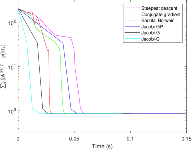
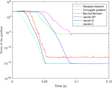
Figure 1. Experimental results for Example 8.1

Example 8.2.

We consider the JATD problem in (3.4) with $d=4$, $n_{1}=n_{2}=5$, $n_{3}=n_{4}=6$ and $r=5$. Let $L=1$ and $\alpha_{1}=1$. Let $\boldsymbol{\mathcal{A}}=\boldsymbol{\mathcal{D}}\mathop{\bullet_{1}}\boldsymbol{U}^{(1)}\mathop{\bullet_{2}}\boldsymbol{U}^{(2)}\mathop{\bullet_{3}}\boldsymbol{U}^{(3)}\mathop{\bullet_{4}}\boldsymbol{U}^{(4)}+\frac{\boldsymbol{\mathcal{E}}}{\|\boldsymbol{\mathcal{E}}\|}$, where $\boldsymbol{\mathcal{D}}$ is a diagonal tensor with $\mathcal{D}_{jjjj}=\sqrt{j}+j\mathbf{i}$ for $1\leq j\leq n_{\rm min}=5$, $\boldsymbol{U}^{(p)}\in\mathbb{C}^{n_{p}\times n_{p}}$, $p=1,2,3,4$, are random unitary matrices, and $\boldsymbol{\mathcal{E}}=\textsf{randn}(n_{1},n_{2},n_{3},n_{4})+\mathbf{i}*\textsf{randn}(n_{1},n_{2},n_{3},n_{4})$. It can be calculated that the initial ratio $\texttt{Rat}=0.0026$. In Jacobi-MG, we choose the parameter $\delta=\frac{1}{10}\sqrt{\frac{2}{dn_{\rm max}(n_{\rm max}-1)}}$. The results of $\|\boldsymbol{\mathcal{A}}\|^{2}-f(\boldsymbol{\omega}_{k})$ and $\|\mathop{{\operator@font grad}}f(\boldsymbol{\omega}_{k})\|$ with respect to the running time are shown in Figure 2. In particular, all the algorithms in Figure 2 arrive at the same ratio $\texttt{Rat}=0.9870$.

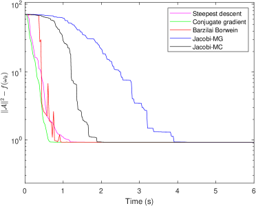
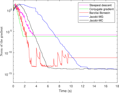
Figure 2. Experimental results for Example 8.2

Example 8.3.

We consider the JATD problem in (3.4) with $d=4$, $n_{1}=n_{2}=n_{3}=n_{4}=3$ and $r=2$. Let $L=1$ and $\alpha_{1}=1$. Let $\boldsymbol{\mathcal{A}}=\boldsymbol{\mathcal{A}}^{\Re}+\mathbf{i}*\boldsymbol{\mathcal{A}}^{\Im}$, where $\boldsymbol{\mathcal{A}}^{\Re}$ and $\boldsymbol{\mathcal{A}}^{\Im}$ are generated randomly using $\textsf{round}(1+\textsf{rand}(n_{1},n_{2},n_{3},n_{4}))$, in which $\textsf{round}(\cdot)$ is the same as that in MATLAB. It can be calculated that the initial ratio $\texttt{Rat}=0.0328$. In Jacobi-MG, we choose the parameter $\delta=\frac{1}{10}\sqrt{\frac{2}{dn_{\rm max}(n_{\rm max}-1)}}$. The results of $\|\boldsymbol{\mathcal{A}}\|^{2}-f(\boldsymbol{\omega}_{k})$ and $\|\mathop{{\operator@font grad}}f(\boldsymbol{\omega}_{k})\|$ with respect to the running time are shown in Figure 3. In particular, all the algorithms in Figure 3 arrive at the same ratio $\texttt{Rat}=0.9196$.

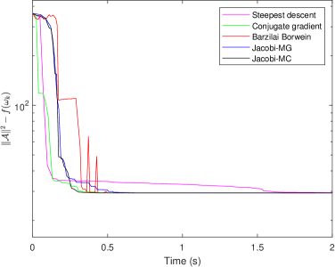
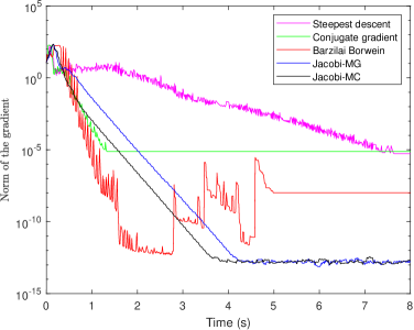
Figure 3. Experimental results for Example 8.3

The results of the above examples demonstrate the efficiency and effectiveness of the tested Jacobi-type algorithms. Compared with the first-order Riemannian optimization methods, the tested Jacobi-type algorithms have much better performances in the convergence to stationary points, since the norm of the gradient for Jacobi-type algorithms is smaller from Figures 1, 2 and 3. On the other hand, in Jacobi-G, Jacobi-MG and Jacobi-GP algorithms, they need to compute the Riemannian gradient and check the gradient inequality (5.1) or (6.2) in each iteration, and thus cost more elapsed time. This is also consistent with our experimental results in Figures 1, 2 and 3.

9. Conclusion

We considered two general classes of homogeneous polynomials with orthogonality constraints, the HPOSM problem (1.1) and HPOSM-P problem (1.2), which include as special cases the JATD-S and JATD problems. We proved some new convergence results for the Jacobi-G algorithm on the unitary group, which is to solve the JATD-S problem. We then proposed the Jacobi-MG algorithm on the product of unitary groups to solve the JATD problem, and also obtained several new convergence results. Moreover, as a generalization of the Jacobi-PC algorithm proposed in [32] and the JLROA-GP algorithm proposed in [34], we formulated the Jacobi-GP and Jacobi-MGP algorithms in the general case to solve the HPOSM problem (1.1) and HPOSM-P problem (1.2), and these two new proximal variants are proved to have global and weak convergence properties. In future work, it may be interesting to consider the following two questions: (i) how to establish the global convergence of Jacobi-G algorithm for JATD-S problem with complex matrices or order-$3$ complex tensors, or order-$4$ real symmetric tensors without any condition; (ii) how to solve the subproblem in Jacobi-G algorithm, if the subproblem can only be represented as the sum of a finite number of quadratic forms (not a single quadratic form as we assume in the present paper).

Acknowledgments. The authors would like to thank Prof. Shuzhong Zhang for his insightful discussions and suggestions. We are grateful to the associate editor and the two anonymous reviewers for their useful suggestions and comments, which helped to improve the presentation of the paper.

References

- [1] T. E. Abrudan, J. Eriksson, and V. Koivunen, Steepest descent algorithms for optimization under unitary matrix constraint, IEEE Transactions on Signal Processing 56 (2008), no. 3, 1134–1147.
- [2] P.-A. Absil, C.G. Baker, and K. A. Gallivan, Trust-region methods on Riemannian manifolds, Foundations of Computational Mathematics 7 (2007), no. 3, 303–330.
- [3] P.-A. Absil, R. Mahony, and B. Andrews, Convergence of the iterates of descent methods for analytic cost functions, SIAM Journal on Optimization 16 (2005), no. 2, 531–547.
- [4] P.-A. Absil, R. Mahony, and R. Sepulchre, Optimization Algorithms on Matrix Manifolds, Princeton University Press, Princeton, NJ, 2008.
- [5] B. W. Bader, T. G. Kolda, et al., Matlab tensor toolbox version 2.6, Available online, February 2015, http://www.sandia.gov/~tgkolda/TensorToolbox/.
- [6] N. Boumal, An Introduction to Optimization on Smooth Manifolds, Cambridge University Press, Cambridge, 2023.
- [7] N. Boumal, B. Mishra, P.-A. Absil, and R. Sepulchre, Manopt, a matlab toolbox for optimization on manifolds, Journal of Machine Learning Research 15 (2014), 1455–1459.
- [8] D. Brandwood, A complex gradient operator and its application in adaptive array theory, IEE Proceedings H - Microwaves, Optics and Antennas 130 (1983), no. 1, 11–16.
- [9] J. F. Cardoso and A. Souloumiac, Blind beamforming for non-gaussian signals, IEE Proceedings F (Radar and Signal Processing) 6 (1993), no. 140, 362–370.
- [10] J. Chen and Y. Saad, On the tensor SVD and the optimal low rank orthogonal approximation of tensors, SIAM Journal on Matrix Analysis and Applications 30 (2009), no. 4, 1709–1734.
- [11] P. Comon, Independent component analysis, a new concept?, Signal Processing 36 (1994), no. 3, 287–314.
- [12] P. Comon and C. Jutten (eds.), Handbook of Blind Source Separation, Academic Press, Oxford, 2010.
- [13] L. De Lathauwer, B. De Moor, and J. Vandewalle, Blind source separation by simultaneous third-order tensor diagonalization, 1996 8th European Signal Processing Conference (EUSIPCO 1996), 1996, pp. 1–4.
- [14] by same author, Independent component analysis and (simultaneous) third-order tensor diagonalization, IEEE Transactions on Signal Processing 49 (2001), no. 10, 2262–2271.
- [15] H. De Sterck and A. J. M. Howse, Nonlinearly preconditioned L-BFGS as an acceleration mechanism for alternating least squares, with application to tensor decomposition, Numerical Linear Algebra with Applications 25 (2018), e2202.
- [16] A. Edelman, T. A. Arias, and S. T. Smith, The geometry of algorithms with orthogonality constraints, SIAM Journal on Matrix Analysis and Applications 20 (1998), no. 2, 303–353.
- [17] L. Eldén and H. Park, A procrustes problem on the stiefel manifold, Numerische Mathematik 82 (1999), no. 4, 599–619.
- [18] L. Eldén and B. Savas, A Newton-Grassmann method for computing the best multilinear rank-(, , ) approximation of a tensor, SIAM Journal on Matrix Analysis and Applications 31 (2009), no. 2, 248–271.
- [19] W. Gander, G. H. Golub, and U. von Matt, A constrained eigenvalue problem, Linear Algebra and Its Applications 114-115 (1989), 815–839.
- [20] B. Gao, X. Liu, X. Chen, and Y. Yuan, A new first-order algorithmic framework for optimization problems with orthogonality constraints, SIAM Journal on Optimization 28 (2018), no. 1, 302–332.
- [21] G. H. Golub and C. F. Van Loan, Matrix Computations, third ed., Johns Hopkins University Press, 1996.
- [22] S. He, Z. Li, and S. Zhang, Approximation algorithms for homogeneous polynomial optimization with quadratic constraints, Mathematical Programming, Series B 125 (2010), no. 2, 353–383.
- [23] S. Hu, An inexact augmented Lagrangian method for computing strongly orthogonal decompositions of tensors, Computational Optimization and Applications 75 (2020), 701–737.
- [24] S. Hu and K. Ye, Linear convergence of an alternating polar decomposition method for low rank orthogonal tensor approximations, Mathematical Programming, Series A (2022), https://doi.org/10.1007/s10107-022-01867-8.
- [25] M. Ishteva, P.-A. Absil, and P. Van Dooren, Jacobi algorithm for the best low multilinear rank approximation of symmetric tensors, SIAM Journal on Matrix Analysis and Applications 2 (2013), no. 34, 651–672.
- [26] M. Ishteva, P.-A. Absil, S. Van Huffel, and L. De Lathauwer, Best low multilinear rank approximation of higher-order tensors, based on the Riemannian trust-region scheme, SIAM Journal on Matrix Analysis and Applications 32 (2011), no. 1, 115–135.
- [27] B. Jiang and Y. H. Dai, A framework of constraint preserving update schemes for optimization on Stiefel manifold, Mathematical Programming, Series A 153 (2015), no. 2, 535–575.
- [28] T. G. Kolda and B. W. Bader, Tensor decompositions and applications, SIAM Review 51 (2009), no. 3, 455–500.
- [29] S. G. Krantz, Function Theory of Several Complex Variables, AMS Chelsea Publishing, Providence, RI, 2001.
- [30] S. G. Krantz and H. R. Parks, A Primer of Real Analytic Functions, Birkhäuser Boston, 2002.
- [31] R. Lai and S. Osher, A splitting method for orthogonality constrained problems, Journal of Scientific Computing 58 (2014), no. 2, 431–449.
- [32] J. Li, K. Usevich, and P. Comon, Globally convergent Jacobi-type algorithms for simultaneous orthogonal symmetric tensor diagonalization, SIAM Journal on Matrix Analysis and Applications 39 (2018), no. 1, 1–22.
- [33] by same author, On the convergence of Jacobi-type algorithms for independent component analysis, 2020 IEEE 11th Sensor Array and Multichannel Signal Processing Workshop (SAM), IEEE, 2020, pp. 1–5.
- [34] by same author, Jacobi-type algorithm for low rank orthogonal approximation of symmetric tensors and its convergence analysis, Pacific Journal of Optimization 17 (2021), no. 3, 357–379.
- [35] J. Li and S. Zhang, Polar decomposition based algorithms on the product of Stiefel manifolds with applications in tensor approximation, arXiv:1912.10390v2 (2020).
- [36] Z. Li, S. He, and S. Zhang, Approximation methods for polynomial optimization: Model, Algorithms, and Applications, 2012.
- [37] C. Ling, J. Nie, L. Qi, and Y. Ye, Biquadratic optimization over unit spheres and semidefinite programming relaxations, SIAM Journal on Optimization 20 (2009), no. 3, 1286–1310.
- [38] S. Łojasiewicz, Ensembles semi-analytiques, IHES notes (1965).
- [39] by same author, Sur la géométrie semi- et sous-analytique, Annales de l’institut Fourier 43 (1993), no. 5, 1575–1595.
- [40] Z. Q. Luo and S. Zhang, A semidefinite relaxation scheme for multivariate quartic polynomial optimization with quadratic constraints, SIAM Journal on Optimization 20 (2010), no. 4, 1716–1736.
- [41] J. H. Manton, Modified steepest descent and newton algorithms for orthogonally constrained optimisation. part I. the complex stiefel manifold, Proceedings of the Sixth International Symposium on Signal Processing and its Applications, vol. 1, 2001, pp. 80–83.
- [42] C. D. M. Martin and C. F. Van Loan, A Jacobi-type method for computing orthogonal tensor decompositions, SIAM Journal on Matrix Analysis and Applications 30 (2008), no. 3, 1219–1232.
- [43] J. Nie and Z. Yang, Hermitian tensor decompositions, SIAM Journal on Matrix Analysis and Applications 41 (2020), no. 3, 1115–1144.
- [44] B. Pesquet-Popescu, J. C. Pesquet, and A. P. Petropulu, Joint singular value decomposition-a new tool for separable representation of images, in Proceedings of the IEEE International Conference on Image Processing, Thessaloniki, Greece, 2001, pp. 569–572.
- [45] R. Schneider and A. Uschmajew, Convergence results for projected line-search methods on varieties of low-rank matrices via Łojasiewicz inequality, SIAM Journal on Optimization 25 (2015), no. 1, 622–646.
- [46] A. Uschmajew, A new convergence proof for the higher-order power method and generalizations, Pacific Journal of Optimization 11 (2015), no. 2, 309–321.
- [47] K. Usevich, J. Li, and P. Comon, Approximate matrix and tensor diagonalization by unitary transformations: convergence of Jacobi-type algorithms, SIAM Journal on Optimization 30 (2020), no. 4, 2998–3028.
- [48] Z. Wen and W. Yin, A feasible method for optimization with orthogonality constraints, Mathematical Programming, Series A 142 (2013), no. 1-2, 397–434.
- [49] Y. Yang, The Epsilon-alternating least squares for orthogonal low-rank tensor approximation and its global convergence, SIAM Journal on Matrix Analysis and Applications 41 (2020), no. 4, 1797–1825.