Enhanced Sensitivity of Degenerate System Made of Two Unstable Resonators Coupled by Gyrator Operating at an Exceptional Point

Abstract

We demonstrate that a circuit comprising two unstable LC resonators coupled via a gyrator supports an exceptional point of degeneracy (EPD) with purely real eigenfrequency. Each of the two resonators includes either a capacitor or an inductor with a negative value, showing purely imaginary resonance frequency when not coupled to the other via the gyrator. With external perturbation imposed on the system, we show analytically that the resonance frequency response of the circuit follows the square-root dependence on perturbation, leading to possible sensor applications. Furthermore, the effect of small losses in the resonators is investigated, and we show that losses lead to instability. In addition, the EPD occurrence and sensitivity are demonstrated by showing that the relevant Puiseux fractional power series expansion describes the eigenfrequency bifurcation near the EPD. The EPD has the great potential to enhance the sensitivity of a sensing system by orders of magnitude. Making use of the EPD in the gyrator-based circuit, our results pave the way to realize a new generation of high-sensitive sensors to measure small physical or chemical perturbations.

I Introduction

An exceptional point of degeneracy (EPD) is a point in parameter space at which the eigenmodes of the circuit, namely the eigenvalues and the eigenvectors, coalesce simultaneously [1, 2, 3, 4]. As the remarkable feature of an EPD is the strong full degeneracy of at least two eigenmodes, as mentioned in [5], the significance of referring to it as a “degeneracy” is here emphasized, hence including "D" in EPD. An EPD in the system is reached when the system matrix is similar to a matrix that contains a non-trivial Jordan block. EPD-induced sensitivity according to the concept of parity-time (PT) symmetry in multiple coupled resonators has been studied [6, 7, 8]. Also, the electronic circuits with EPD based on PT symmetry have been expressed in [9, 10] and then more developed in [11, 12] where the circuits are made of two coupled resonators with gain-loss symmetry and a proper combination of parameters leads to an EPD. Primarily, it has been confirmed that the eigenvalues bifurcation feature at EPD can significantly increase the effect of external perturbation; namely, the sensitivity of resonance frequency to components value perturbations can be enhanced. Moreover, frequency splitting happens at degenerate frequencies of the system where eigenmodes coalesce, and this feature at EPDs has been investigated to conceive a new generation of sensors [13, 14, 15, 16]. The resulting perturbation leads to a shift in the system resonance frequency that can be recognized and measured using the proper measurement setup [13]. When a second-order EPD at which specifically two eigenstates coalesce is subjected to a small external perturbation, the resulting eigenvalue splitting is proportional to the square root of external perturbation value, which is bigger than the case of linear splitting for conventional degeneracies [17]. The concept of EPD has been employed in various sensing schemes such as optical microcavities [8], optical microdisk [18], electron beam devices [19], mass sensors [20], and bending curvature sensors [21].

The gyrator is a two-terminal element with the property of transmission phase shift in one direction differs by $\pi$ from that for transmission in the other direction [22]. Another property of the gyrator network is that of impedance inversion. The inductance at the output of the gyrator is observed as capacitance at the input port, and a voltage source is transformed to a current source. A relevant alias for the gyrator might be the “dualizer” since it can interchange current and voltage roles and turns an impedance into its dual [23]. Gyrators could be designed directly as integrated circuits [24, 25]. Also, many operational-amplifier (opamp) gyrator circuits have been proposed [26, 27, 28], which can be classified into two types. First, 3-terminal gyrator circuits in which both ports are grounded [26]; second, 4-terminal gyrator circuits in which the output port is floating [27, 28]. Because of the availability of different realizable circuits for gyrators and their versatility for practical circuit devices, gyrator-based circuits may form an essential part of integrated circuit technology in a wide range of applications.

In this paper, we study the second-order EPDs in a gyrator-based sensing circuit as Fig. 1 and explore its enhanced sensitivity (variation in sensor’s resonance frequencies to external perturbations) and its potentials for sensing devices in the vicinity of EPD. Two series LC resonators are coupled in the utilized circuit via an ideal gyrator, as explained in [29]. Contrary to the study in [29], this paper demonstrates the conditions to get the EPD with real eigenfrequency by using unstable resonators. In other words, we study the case of two unstable resonators coupled via an ideal gyrator. A general mathematical approach for constructing lossless circuits for any conceivable Jordan structure has been developed in [30], including the simplest possible circuit as in Fig. 1 and other circuits related to the Jordan blocks of higher dimensions. In addition, important issues related to operational stability, perturbation analysis, and sensitivity analysis are studied in [31], whereas analysis of stability or instability by adding losses to the circuit is not discussed. We show that the gyrator-based circuit can achieve EPD with real eigenfrequency even when two unstable resonators are used in the circuit. Hence, dispersion diagrams correspond to perturbation in the circuit’s parameters show the eigenfrequencies split. Then, we show examples for different cases and analyze the output signal by using time-domain simulations. We then study the impact of small losses in the circuit and explain how they can make it unstable. Besides, we look at the sensitivity of circuit eigenfrequencies to component variations, and we show that the Puiseux fractional power series expansion well approximates the bifurcation of the eigenfrequency diagram near the EPD [32]. The sensitivity enhancement is attributed to the second root topology of the eigenvalues in parameter space, peculiar to the second-order EPD. Lastly, we examine the gyrator-based circuit’s enhanced sensitivity and provide a practical scenario to detect physical parameters variations and material characteristics changes. Besides exploring EPD physics in the gyrator-based circuits, this work is also important for understanding the instability in resonators. The given analysis and circuit show promising potential in the novel ultra high-sensitive sensing applications.

II Gyrator Characteristic

A gyrator is a two-port component that couples an input port to an output port by a gyration resistance value. It is a lossless and storage-less two-port network that converts circuits at the gyrator output into their dual, with respect to the gyration resistance value [33]. For instance, this component can make a capacitive circuit behave inductively, a series LC resonator behave like a parallel LC resonator, and so on. This device allows network realizations of two-port devices, which cannot be realized by just the basic components, i.e., resistors, inductors, capacitors, and transformers. In addition, the gyrator could be considered a more fundamental circuit component than the ideal transformer because an ideal transformer can be made by cascading two ideal gyrators, but a gyrator cannot be made from transformers [22]. The circuit symbol for the ideal gyrator is represented in Fig. 1 (red dashed box), and the defining equations are [22, 34]

$$\begin{cases}v_{2}=R_{g}i_{1}\\ v_{1}=-R_{g}i_{2}\end{cases}$$ (1)

where $R_{g}$ is called gyration resistance and has a unit of Ohm. A gyrator is a nonreciprocal two-port network represented by an asymmetric impedance matrix $\mathbf{\underline{Z}}$ as [34]

$$\mathbf{\underline{Z}}=\left[\begin{array}[]{cc}0&-R_{g}\\ R_{g}&0\end{array}\right].$$ (2)

III EPD Condition in The Lossless Gyrator-Based Circuit

This section provides an analysis of a gyrator-based circuit in which two series LC resonators are coupled via an ideal gyrator as illustrated in 1. We first assume that all components are ideal, and the circuit does not contain any resistance. The circuit resembles the one in [29], but here the two resonance angular frequencies $\omega_{01}=1/\sqrt{C_{1}L_{1}}$, and $\omega_{02}=1/\sqrt{C_{2}L_{2}}$ of the two uncoupled resonators are imaginary with a negative sign (also the counterpart with the positive sign is a resonance), since we consider three cases: (i) both $L_{1}$ and $L_{2}$ are negative while the capacitors have a positive value, (ii) both $C_{1}$ and $C_{2}$ are negative while the inductors have a positive value, and (iii) $L_{1}$($C_{1}$) and $C_{2}$($L_{2}$) are negative while other elements have a positive value. Then we investigate the possibility of the occurring EPD in the cases just mentioned. In the past years, EPDs have been found by using balanced loss and gain in a PT symmetry scheme [35, 10, 8]. More recently, EPDs have also been found in systems with time-periodic modulation [36, 37]. Here, we obtain EPDs by using the negative inductance and capacitance in the gyrator-based circuit, constituting a new class of EPD-based circuits.

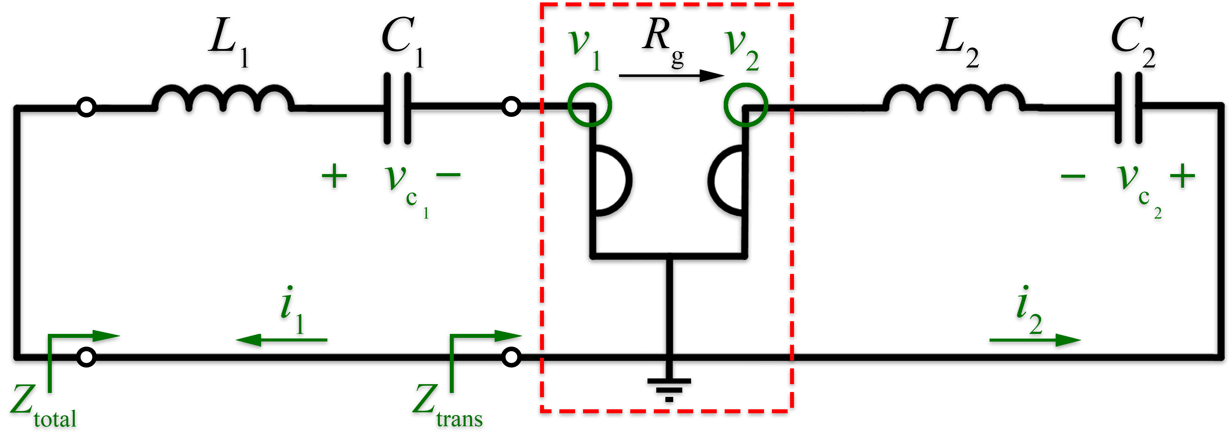
Figure 1: The schematic illustration of the proposed gyrator-based circuit with the ideal gyrator indicated by the red dashed box. In this circuit, two different (unstable) LC resonators are embedded in a series configuration, coupled via an ideal gyrator.

We consider the Kirchhoff voltage law equations in the time-domain for two loops of the circuit in Fig. 1. In order to find the solution of the circuit differential equations, it is convenient to define the state vector as $\boldsymbol{\Psi}(t)\equiv[Q_{1},Q_{2},\dot{Q}_{1},\dot{Q}_{2}]^{T}$, where $T$ denotes the transpose operator. The state vector consists of stored charges in the capacitors $Q_{n}=\int i_{n}dt=C_{n}v_{c_{n}}$, and their time derivative (currents) $\dot{Q}_{n}=i_{n}$, $n=1,\ldots,4.$ We utilize then the Liouvillian formalism for this circuit as [29]

$$\mathcal{\mathrm{\frac{d\boldsymbol{\Psi}(t)}{dt}=\mathbf{\underline{M}}\boldsymbol{\Psi}(t),\;}\mathbf{\underline{M}}}=\left(\begin{array}[]{cccc}0&0&1&0\\ 0&0&0&1\\ -\omega_{01}^{2}&0&0&\frac{R_{g}}{L_{1}}\\ 0&-\omega_{02}^{2}&-\frac{R_{g}}{L_{2}}&0\end{array}\right),$$ (3)

where $\underline{\mathbf{M}}$ is the $4\times 4$ circuit matrix. Assuming time harmonic dependence of the form $Q_{n}\varpropto e^{j\omega t}$, we obtain the characteristic equation allowing us to find the eigenfrequencies by solving $\det(\underline{\mathbf{M}}-j\omega\underline{\mathbf{I}})=0$, where $\underline{\mathbf{I}}$ is the identity matrix. The corresponding characteristic equation of the circuit is

$$\omega^{4}-\omega^{2}\left(\omega_{01}^{2}+\omega_{02}^{2}+\frac{R_{g}^{2}}{L_{1}L_{2}}\right)+\omega_{01}^{2}\omega_{02}^{2}=0,$$ (4)

where any solution $\omega$ is an eigenfrequency of the circuit. In the case of $R_{g}=0$, the two resonators are uncoupled, and the circuit has two eigenfrequency pairs of $\omega_{1,3}=\pm\omega_{01}$, and $\omega_{2,4}=\pm\omega_{02},$ that are purely imaginary (in contrast to the case studies in [29], where the resonance frequencies have real values). All the $\omega$’s coefficients of the characteristic equation are real, so $\omega$ and $\omega^{*}$ are both roots of the characteristic equation, where * indicates the complex conjugate operator. Moreover, it is a quadratic equation in $\omega^{2}$; therefore, $\omega$ and $-\omega$ are both solutions of the Eq. (4). As we mentioned before, we only consider unstable resonators, i.e., resonators with imaginary resonance frequency. Therefore, only one circuit element in each resonator should have a negative value, leading to $\omega_{01}^{2}$ and $\omega_{02}^{2}$ with negative values. After finding the solutions of the characteristic equation, the angular eigenfrequencies (resonance frequencies) of the circuit are expressed as

$$\omega_{1,3}=\pm\sqrt{a+b},\;\omega_{2,4}=\pm\sqrt{a-b},$$ (5)

where

$$a=\frac{1}{2}\left(\omega_{01}^{2}+\omega_{02}^{2}+\omega_{g}^{2}\right),$$ (6)

$$\begin{array}[]{c}b^{2}=a^{2}-\omega_{01}^{2}\omega_{02}^{2}\end{array},$$ (7)

where it has been convenient to define $\omega_{g}^{2}=R_{g}^{2}/(L_{1}L_{2})$, that may be positive or negative depending on the considered case. According to Eq. (5), the EPD condition requires

$$b=0,$$ (8)

leading to an EPD angular frequency $\omega_{\mathit{e}}=\sqrt{a}$ (with its negative pair $-\omega_{\mathit{e}}$). According to Eq. (7), the EPD condition is rewritten as $a^{2}=\omega_{01}^{2}\omega_{02}^{2}.$ As in [29], we consider positive values for $a$ to have a real EPD angular frequency $\omega_{\mathit{e}}$ , so we have

$$\omega_{01}^{2}+\omega_{02}^{2}+\omega_{g}^{2}>0.$$ (9)

Finally, the EPD frequency is calculated by using Eqs. (6), (7), and (8) as

$$\begin{array}[]{c}\omega_{\mathit{e}}=\sqrt{\frac{1}{2}\left(\omega_{01}^{2}+\omega_{02}^{2}+\omega_{g}^{2}\right)}.\end{array}$$ (10)

The last equation can also be rewritten as $\omega_{\mathit{e}}=\sqrt[4]{\omega_{01}^{2}\omega_{02}^{2}}$, with the quartic square root defined by taking the positive value; in other words, if we consider that the two unstable frequencies have the following purely imaginary expression, $\omega_{01}=-j/\sqrt{|C_{1}L_{1}|}$ and $\omega_{02}=-j/\sqrt{|C_{2}L_{2}|}$, the EPD frequency can be expressed as $\omega_{\mathit{e}}=\sqrt{-\omega_{01}\omega_{02}}$. We obtain the desired value of a real EPD frequency by optimizing the values of the components in the circuit. Theoretically, the utilized optimization method is not critical, and merely we need to found the proper solution for Eq. (8). Obviously, practical limitations also affect the selection of suitable constraints for optimization. In the particular case the two circuits are identical, one has $\omega_{0}^{2}\equiv\omega_{01}^{2}=\omega_{02}^{2}=1/(LC)<0$, and the EPD condition (8) reduces to $4\omega_{0}^{2}=-\omega_{g}^{2},$that in turns leads to the EPD angular frequency $\begin{array}[]{c}\omega_{\mathit{e}}=\sqrt{-\omega_{0}^{2}}\end{array}$. In the following subsections, we analyze the circuit in three different cases, i.e., the three different assumptions mentioned earlier.

III-A Negative Inductances $L_{1}$ and $L_{2}$

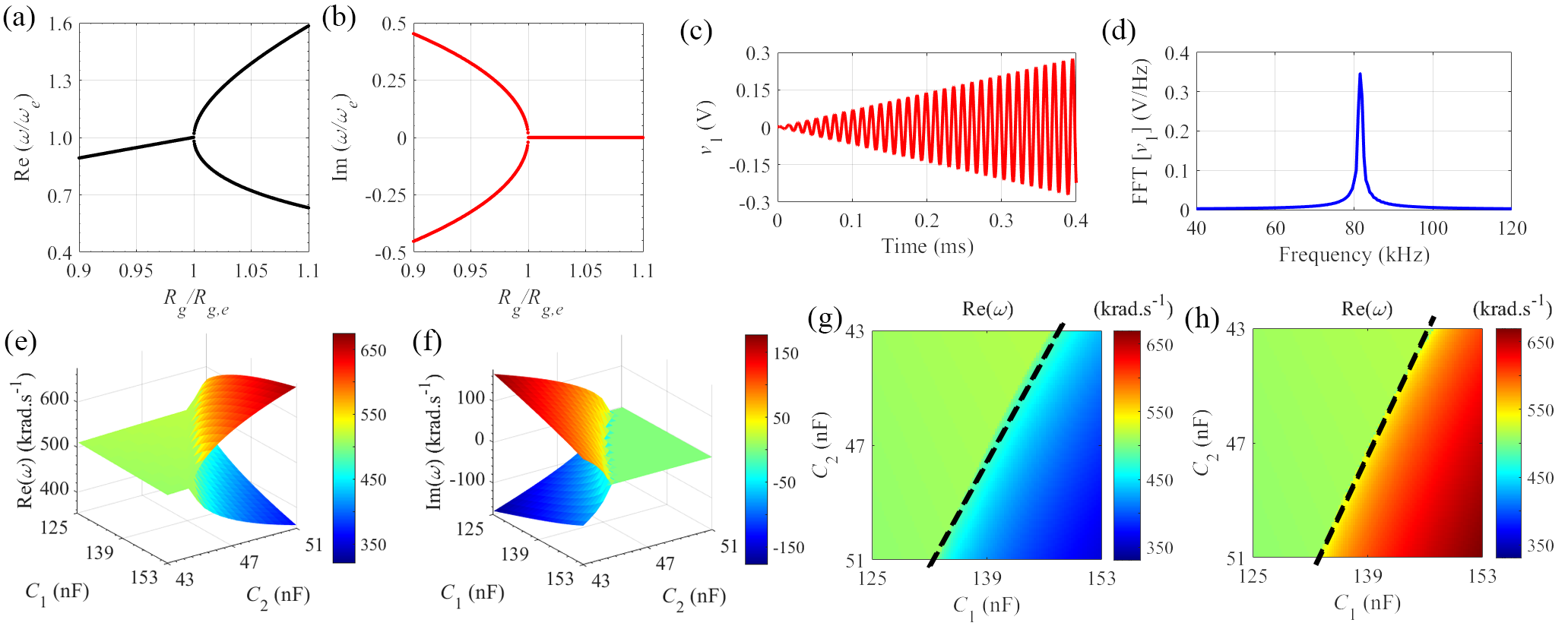
Figure 2: The sensitivity of the (a) real and (b) imaginary parts of the eigenfrequencies to gyration resistance perturbation. Voltage $v_{1}(t)$ under the EPD condition in the (c) time-domain, and (d) frequency-domain. The frequency-domain result is calculated from $40\mathrm{\>kHz}$ to $120\>\mathrm{kHz}$ by applying an FFT with $10^{6}$ samples in the time window of $0\>\mathrm{ms}$ to $0.4\>\mathrm{ms}$. The three-dimensional plot of the (e) real and (f) imaginary parts of the eigenfrequencies to $C_{1}$ and $C_{2}$ perturbation. The real part of eigenfrequencies for (g) higher and (h) lower value of resonance frequencies which colormap show the resonance frequency value. The black dashed line in these plots shows the EPD.

As a first case, we consider a negative value for both inductances and a positive value for both capacitances; hence, in this case $\omega_{g}^{2}>0$. According to the required condition for EPD expressed in Eq. (8) and by using Eq. (7), the first and second terms in Eq. (6) are negative and the third term is positive. Eq. (10) shows that, if $\left|\omega_{01}^{2}+\omega_{02}^{2}\right|<\omega_{g}^{2}$ we obtain a real value for EPD frequency, and if $\left|\omega_{01}^{2}+\omega_{02}^{2}\right|>\omega_{g}^{2}$, the EPD frequency yields an imaginary value.

We explain the procedure to obtain an EPD in this circuit by presenting an example. Various combinations of values for the circuit’s components can satisfy the EPD condition demonstrated in Eq. (8), and here as an example, we consider this set of values: $L_{1}=-47\mathrm{\>\mu H}$, $L_{2}=-47\mathrm{\>\mu H}$, $C_{2}=47\mathrm{\>nF}$, and $R_{g}=50\>\Omega$. Then, the capacitance of the first resonator is determined by solving the resulting quadratic equation from the EPD condition demonstrated in Eq. (8). In this example, we consider $C_{1}$ as a sensing capacitance of the circuit, which has a positive value and it can detect variations in environmental parameters and transform them into electrical quantities. According to Eq. (8), after solving the quadratic equation, two different values for capacitance in the first resonator are calculated, and we consider $C_{1,\mathit{e}}=139.17\>\mathrm{nF}$ for the presented example. According to the calculated values for components, both $\omega_{01}^{2}$ and $\omega_{02}^{2}$ have negative values, with $\omega_{01}=-j391\>\mathrm{krad/s}$, and $\omega_{02}=-j672.82\>\mathrm{krad/s}$, leading to a positive result for $a$ in Eq. (6) and real EPD angular frequency $\omega_{\mathit{e}}=512.9\mathrm{\>krad/s}$. The results in Figs. 2(a), and (b) show the real and imaginary parts of perturbed eigenfrequencies obtained from the eigenvalue problem when $R_{g}$ of the ideal gyrator is perturbed, revealing the high sensitivity to perturbations.

To investigate the time-domain behavior of the circuit under EPD conditions, we used the Keysight Advanced Design System (ADS) circuit simulator. The transient behavior of the coupled resonators with the ideal gyrator is simulated using the time-domain solver with an initial condition $v_{c_{1}}(0)=1\>\mathrm{mV}$, where $v_{c_{1}}(t)$ is the voltage of the capacitor in the left resonator. Fig. 2(c) shows the time-domain simulation results of the voltage $v_{1}(t)$, where $v_{1}(t)$ is the voltage at the gyrator input port (see Fig. 1). The extracted result is obtained in the time span of $0$ ms to $0.4$ ms. The solution of the eigenvalue problem in the Eq. (3) and at the EPD is different from any other regular frequency in the dispersion diagram since the system matrix contains repeated eigenvalues associated with one eigenvector. Thus, the time-domain response of the circuit at the second-order EPD is expected to be in the form of $\boldsymbol{\Psi}(t)\propto te^{j\omega_{\mathit{e}}t}$, as it is indeed shown in Fig. 2(c). The voltage grows linearly by increasing time, whereas the oscillation frequency is constant. This remarkable feature is peculiar to an EPD, and it is the result of coalescing eigenvalues and eigenvectors that also corresponds to a double pole in the circuit (or zero, depending on what is observed). We take a fast Fourier transform (FFT) of the voltage $v_{1}(t)$ to show the frequency spectrum, and the calculated result is illustrated in Fig. 2(d). The result is calculated from $40\mathrm{\>kHz}$ to $120\>\mathrm{kHz}$ by applying an FFT with $10^{6}$ samples in the time window of $0\>\mathrm{ms}$ to $0.4\>\mathrm{ms}$. The numerically observed oscillation angular frequency is $f_{0}=\omega_{o}/(2\pi)=81.63\mathrm{\>kHz}$, that shows the frequency corresponds to the maximum value in 2(d). The numerically obtained value is in good agreement with the theoretical value calculated above.

So far, we have used the gyrator-based circuit to measure the perturbation near EPD by varying the gyrator resistance. Next, we analyze the circuit’s sensitivity to independent perturbations in the positive values of both capacitances. We change the capacitance value on each resonator independently and calculate the eigenfrequencies’ real and imaginary parts. The three-dimensional result for the calculated eigenfrequencies is illustrated in Figs. 2(e), and (f). The elevation value of any point on the surface shows the eigenfrequency, and the associated color helps to recognize it conveniently. In these figures, only the two solutions with $\mathrm{Re}(\omega)>0$ are illustrated. Although the resonance frequency of each resonator in this paper is imaginary, in the specific range of $C_{1}$ and $C_{2}$, the EPD frequency is purely real. To utilize these calculated results, the flat version of the three-dimensional diagram for the real part is provided in Figs. 2(g), and (h) for higher and lower eigenfrequency. These figures can help designers in the design procedure to select the proper value for components to achieve the desired real resonance frequency. The intersection of two surfaces (eigenfrequencies surface and surface of constant $z$ plane) is a one-dimensional curve. Therefore, there is a different set of values for capacitances to make oscillation at a certain frequency. Moreover, the intersection of the higher eigenfrequencies surface and lower eigenfrequencies surface indicates the possible EPD that various combinations of capacitances values can yield. Designers can use these figures and pick a proper value in the design steps according to their practical limitations.

III-B Negative Capacitances $C_{1}$ and $C_{2}$

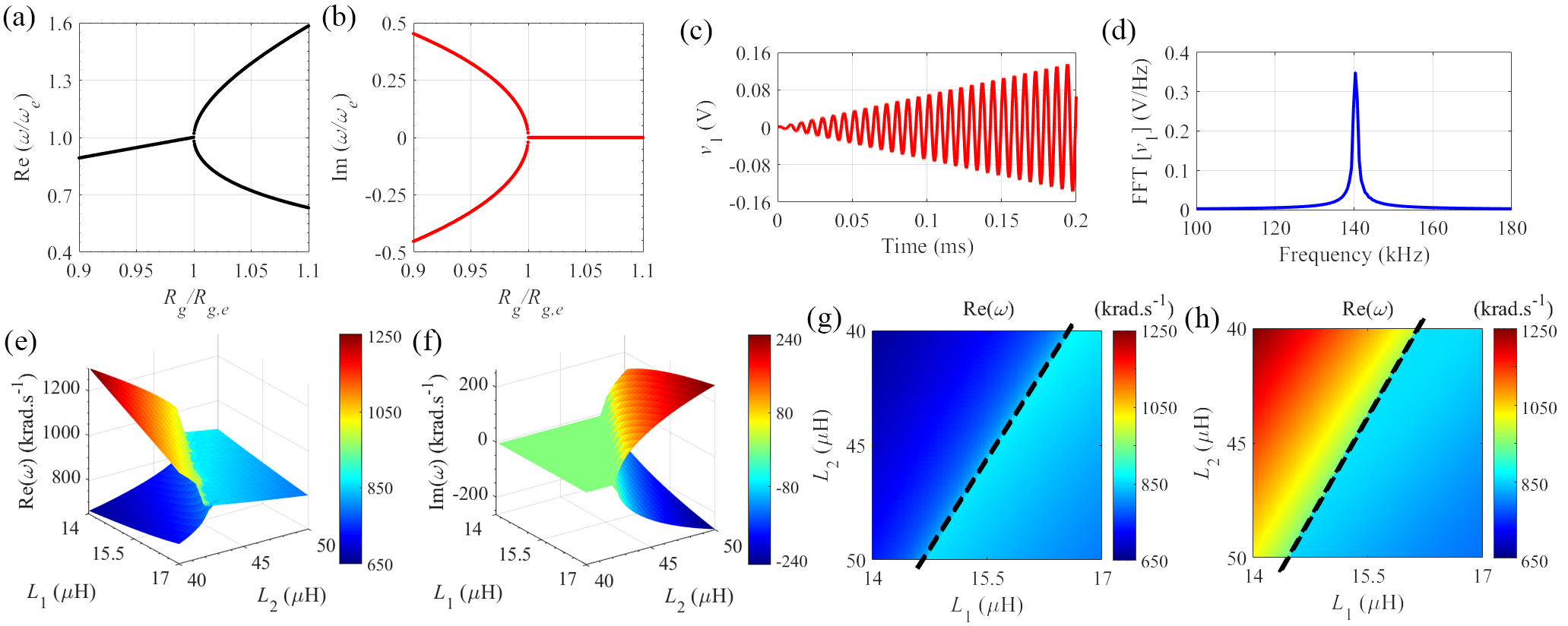
Figure 3: The sensitivity of the (a) real and (b) imaginary parts of the eigenfrequencies to gyration resistance perturbation. Voltage $v_{1}(t)$ under the EPD condition in the (c) time-domain, and (d) frequency-domain. The frequency-domain result is calculated from $100\mathrm{\>kHz}$ to $180\>\mathrm{kHz}$ by applying an FFT with $10^{6}$ samples in the time window of $0\>\mathrm{ms}$ to $0.2\>\mathrm{ms}$. The three-dimensional plot of the (e) real and (f) imaginary parts of the eigenfrequencies to $L_{1}$ and $L_{2}$ perturbation. The real part of eigenfrequencies for (g) higher and (h) lower value of resonance frequencies which colormap show the resonance frequency value. The black dashed line in these plots shows the EPD.

In the following section, we consider another condition in which negative capacitances are used on both resonators; so $\omega_{g}^{2}>0$. Using the mentioned presumption, the first and second terms in Eq. (6) are negative because of the imaginary value of resonance frequencies of resonators, and the third term is positive. So, if the EPD condition is met, the sign of $a$ in Eq. (6) indicates whether the eigenfrequency is real or imaginary. According to Eq. (5), if $\left|\omega_{01}^{2}+\omega_{02}^{2}\right|<\omega_{g}^{2}$ we get a real value for the EPD frequency, and if $\left|\omega_{01}^{2}+\omega_{02}^{2}\right|>\omega_{g}^{2}$, the EPD frequency is imaginary.

Different combinations of values for the circuit’s components can satisfy the EPD condition demonstrated in Eq. (8), and here as an example, we use this set of values: $C_{1}=-47\mathrm{\>nF}$, $C_{2}=-47\mathrm{\>nF},$ $L_{2}=47\mathrm{\>\mu H}$, and $R_{g}=50\>\Omega$. The inductance value on the left resonator is calculated by solving the resulting quadratic equation from Eq. (8). In the presented example, $L_{1}$ can be a sensing inductor in a system. According to Eq. (8), two different values for inductance in the first resonator are calculated after solving the quadratic equation. We consider $L_{1,\mathit{e}}=15.87\mathrm{\>\mu H}$ for this example, so both $\omega_{01}^{2}$ and $\omega_{02}^{2}$ have negative values, with $\omega_{01}=-j1.16\>\mathrm{Mrad/s}$, and $\omega_{02}=-j672.82\>\mathrm{krad/s}$. Then, we obtain a positive value for $a$ in Eq. (6), leading to a real EPD angular frequency of $\omega_{\mathit{e}}=881.6\mathrm{\>krad/s}$. The results in Figs. 3(a), and (b) shows the two branches of the real and imaginary parts of eigenfrequencies obtained by perturbing $R_{g}$ near the value that made the EPD.

The time-domain simulation result by using the Keysight ADS with an initial condition $v_{1}(0)=1\>\mathrm{mV}$ is presented in Fig. 3(c). The voltage $v_{1}(t)$ is calculated in the time interval of $0$ ms to $0.2$ ms. Fig. 3(c) shows $v_{1}(t)$ is growing linearly by increasing time. The growing signal demonstrates the circuit eigenvalues coalesce, and the output rises linearly at the second-order EPD frequency. In order to evaluate the oscillation frequency from the time-domain simulation, we take an FFT of voltage $v_{1}(t)$ from $100\mathrm{\>kHz}$ to $180\>\mathrm{kHz}$ using $10^{6}$ samples in the time window of $0\>\mathrm{ms}$ to $0.2\>\mathrm{ms}$. The calculated spectrum is shown in Fig. 3(d), showing an oscillation frequency of $f_{0}=\omega_{o}/(2\pi)=140.31\mathrm{\>kHz}$, which is in good agreement with the calculated theoretical value obtained from Eq. (10).

In the following step, we investigate the circuit’s sensitivity to independent perturbation in the value of both inductances. The real and imaginary parts of eigenfrequencies are calculated when the values of the inductances are changed. The three-dimensional eigenfrequencies map of the two solutions with $\mathrm{Re}(\omega)>0$ is shown in Figs. 3(e), and (f). In order to provide a better representation, the flat view of the three-dimensional diagram for the real part is shown in Figs. 3(g), and (h) for higher and lower eigenfrequencies.

III-C Negative Inductance on One Side and Negative Capacitance on The Other Side

In this last case, different constraints for components value are considered. We assume a component with a negative value on one side (capacitance/inductance) and the other component with a negative value on the other side (inductance/capacitance); hence, in this case $\omega_{g}^{2}<0$. For instance, we consider a negative inductance on the right resonator and a negative capacitance on the left resonator. It is evident that in this case, we have two unstable resonators when they are uncoupled. When two resonators are coupled, EPD should satisfy Eq. (7). According to Eq. (10), all terms inside the square root are negative, and the sum of negative values is always negative. As a result, it is impossible to achieve an EPD with a real eigenfrequency under the assumption mentioned above. Since we focus on cases with real EPD frequency in this paper, we will skip considering this condition in the rest of the paper.

IV Frequency-Domain Analysis of The Resonances in Lossless Gyrator-Based Circuit

We demonstrate how the EPD regime is associated with a special kind of circuit’s resonance, directly observed in frequency-domain circuit analysis. First, we calculate the transferred impedance on the left port of the gyrator in Fig. 1, which is

$$Z_{trans}(\omega)=\frac{R_{g}^{2}}{Z_{2}(\omega)},$$ (11)

where $Z_{2}(\omega)=j\omega L_{2}+1/(j\omega C_{2})$ is the impedance of LC tank on the right side of the gyrator. The total impedance observed from the input port (see Fig. 1) is

$$Z_{total}(\omega)\triangleq Z_{1}(\omega)+Z_{trans}(\omega)=Z_{1}(\omega)+\frac{R_{g}^{2}}{Z_{2}(\omega)},$$ (12)

where $Z_{1}(\omega)=j\omega L_{1}+1/(j\omega C_{1})$ is the impedance of LC tank on the left side of the gyrator. The complex-valued resonance frequencies of the circuit are calculated by imposing $Z_{total}(\omega)=0$. Fig. 4 shows the zeros of such total impedance $Z_{total}(\omega)$ for various gyration resistance values (arrows represent growing $R_{g}$ values). When considering the EPD gyrator resistance $R_{g}=R_{g,\mathit{e}}=50\,\Omega$, one has $Z_{total}(\omega)\propto(\omega-\omega_{\mathit{e}})^{2}$, i.e., the two zeros coincide with the EPD angular frequency $\omega_{\mathrm{\mathit{e}}}$, that is also the point where the two curves in Fig. 4 meet. For gyrator resistances $R_{g}<R_{g,\mathit{e}}$, the two resonance angular frequencies are complex conjugate, consistent with the result in Fig. 4. Also, for gyrator resistances such that $R_{g}>R_{g,\mathit{e}}$, the two resonance angular frequencies are purely real. In other words, the EPD frequency coincides with double zeros of the frequency spectrum, or double poles, depending on the way the circuit is described.

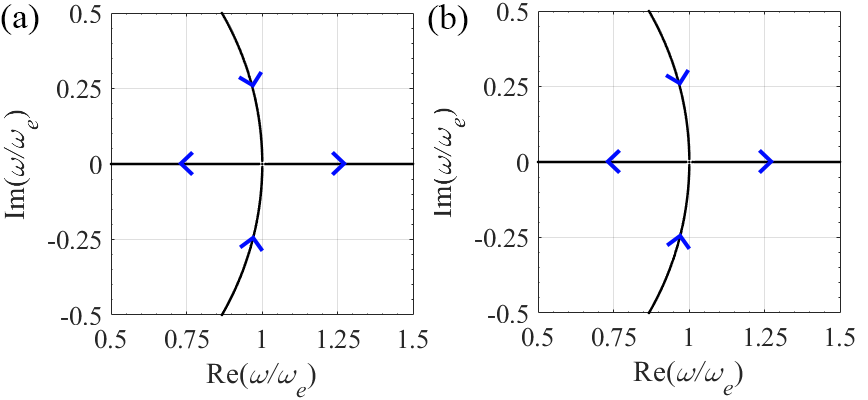
Figure 4: Root locus of zeros of $Z_{total}(\omega)=0$ showing the real and imaginary parts of resonance frequencies of the circuit when varying gyration resistance (arrows represent growing $R_{g}$ values). In these figures, we consider two cases, with a negative value of (a) both inductances and (b) both capacitances, discussed in Section III. At the EPD, the system’s total impedance is $Z_{total}(\omega)\propto(\omega-\omega_{\mathit{e}})^{2}$; hence it exhibits a double zero at $\omega_{\mathit{e}}$.

V EPD in The Lossy Gyrator-Based Circuit

The following section analyzes the EPD condition in the gyrator-based circuit by accounting for series resistors $R_{1}$ and $R_{2}$ in resonators as illustrated in Fig. 5. A procedure analogous to the one discussed earlier, using the same state vector $\boldsymbol{\Psi}\equiv[Q_{1},Q_{2},\dot{Q}_{1},\dot{Q}_{2}]^{T}$, leads to [29]

$$\mathcal{\mathrm{\frac{d\boldsymbol{\Psi}}{dt}=\mathbf{\underline{M}}\boldsymbol{\Psi},\;\;}}\mathbf{\underline{M}}=\left(\begin{array}[]{cccc}0&0&1&0\\ 0&0&0&1\\ -\omega_{01}^{2}&0&-\gamma_{1}&\frac{R_{g}}{L_{1}}\\ 0&-\omega_{02}^{2}&-\frac{R_{g}}{L_{2}}&-\gamma_{2}\end{array}\right).$$ (13)

In the presented lossy circuit matrix, $\gamma_{1}=R_{1}/L_{1}$, and $\gamma_{2}=R_{2}/L_{2}$ determine losses in each resonator. These eigenfrequencies of the circuit are found by solving the below characteristic equation,

$$\begin{array}[]{c}\omega^{4}-j\omega^{3}\left(\gamma_{1}-\gamma_{2}\right)-\omega^{2}\left(\omega_{01}^{2}+\omega_{02}^{2}+\gamma_{1}\gamma_{2}+\frac{R_{g}^{2}}{L_{1}L_{2}}\right)\\ +j\omega\left(\gamma_{1}\omega_{02}^{2}+\gamma_{2}\omega_{01}^{2}\right)+\omega_{01}^{2}\omega_{02}^{2}=0.\end{array}$$ (14)

The coefficients of the odd-power terms of the angular eigenfrequency in the characteristic equation are imaginary; therefore, $\omega$ and $-\omega^{*}$ are both roots of the characteristic equation. In order to obtain a stable circuit with real-valued eigenfrequencies, the coefficients of the odd-power terms in the characteristic equation Eq. (14), $-j(\gamma_{1}-\gamma_{2})$ and $j(\gamma_{1}\omega_{02}^{2}+\gamma_{2}\omega_{01}^{2})$, should vanish, otherwise a complex eigenfrequency is needed to satisfy the characteristic equation. The coefficient of the $\omega^{3}$ term is zero when $\gamma_{1}=\gamma_{2}$, but according to this condition, the coefficient of the $\omega$ term is non-zero because $\omega_{01}^{2}$ and $\omega_{02}^{2}$ are both negative. Moreover, the coefficient of the $\omega$ term never vanishes when both resonators are lossy because both $\omega_{01}^{2}$ and $\omega_{02}^{2}$ have the same sign. Consequently, it is not possible to have all real-valued coefficients in the characteristic polynomials, except when $\gamma_{1}=\gamma_{2}=0$, which corresponds to a lossless circuit.

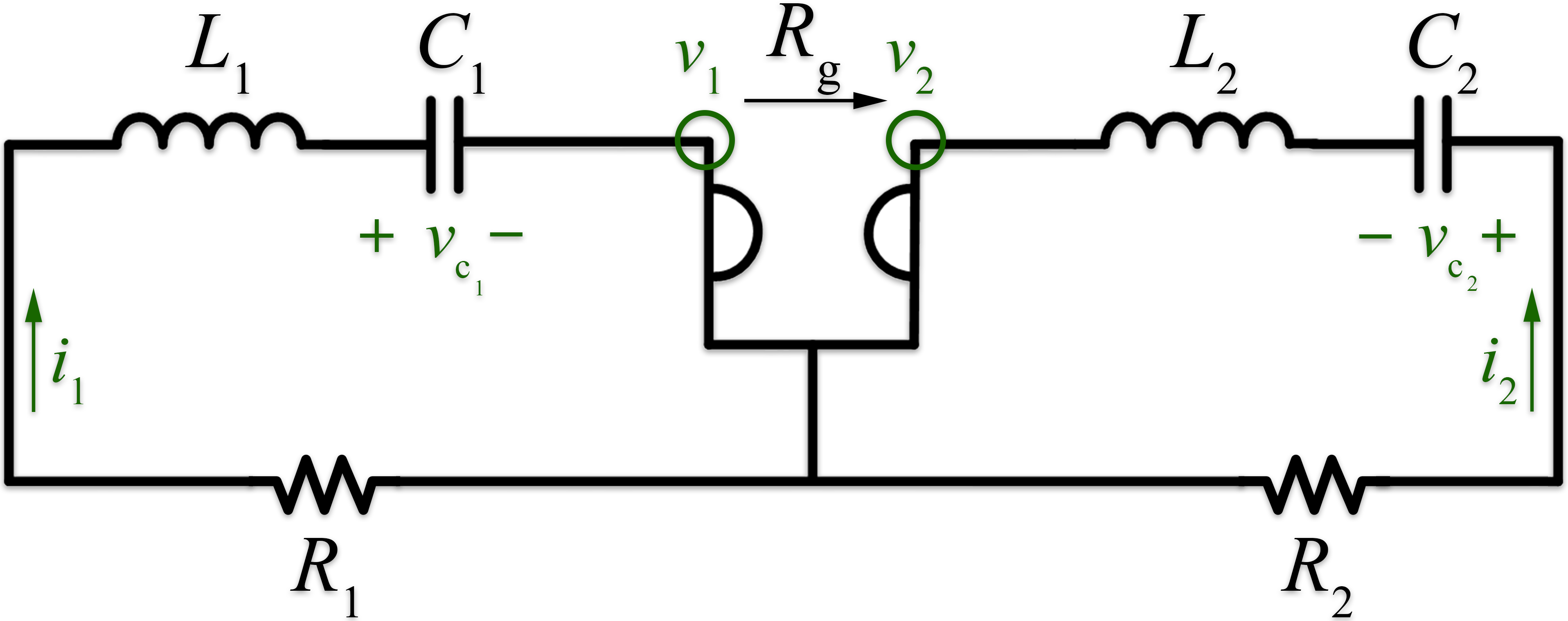
Figure 5: Schematic view of the lossy gyrator-based circuit, with a resistor in each resonator.

V-A RLC Resonators With Negative Inductances $L_{1}$ and $L_{2}$

In the first case, we assume inductances with negative values. In Figs. 6(a) and (b), $\gamma_{1}$ is perturbed while we assume $\gamma_{2}=0$, whereas in Figs. 6(c), and (d), $\gamma_{2}$ is perturbed while $\gamma_{1}=0$. These four figures present the real and imaginary parts of eigenfrequencies when the resistances $R_{1}$ and $R_{2}$ are perturbed individually. We use the same values for the circuit components as already used in the lossless circuit presented in Subsection III-A. The normalization term $\omega_{\mathit{e}}$ is the EPD angular frequency obtained when $\gamma_{1}=\gamma_{2}=0$, which is the same EPD frequency of the lossless circuit. In this case, losses in the circuit are represented by negative $\gamma_{1}$ and $\gamma_{2}$ since $L_{1}$, and $L_{2}$ are negative, so the right half side of the figure axes show the loss and the left half side of the axes represent the gain in the circuit through a negative resistance. In Figs. 6(a)-(d), we recognize the bifurcations of the real and imaginary parts of the eigenfrequencies, so the circuit is extremely sensitive to variations of resistances in the vicinity of EPD. By perturbing $\gamma_{1}$ or $\gamma_{2}$ away from $\gamma_{1}=\gamma_{2}=0$, the circuit becomes unstable, and it begins to self oscillate at a frequency associated with the real part of the unstable angular eigenfrequency. In addition, we show the real and imaginary parts of the eigenfrequencies by separately perturbing the resistances in both sides in 6(e)-(f). The black contour lines in these three-dimensional figures show constant real and imaginary parts of the eigenfrequencies. We observe that by adding either loss or gain, the circuit becomes unstable. Instability in the circuit is not due to the instability of the uncoupled resonators, but rather it is unstable because of the addition of losses, as was the case in [29] for different configurations. When $\gamma_{1}$ or $\gamma_{2}$ is perturbed from the EPD, the oscillation frequency is shifted from the EPD frequency, and it could be measured for sensing applications. The eigenfrequency with a negative imaginary part is associated with an exponentially growing signal (instability). Considering the existence of instability, there are a few possible ways of operations: preventing the system from reaching saturation by switching off the circuit, partially compensating for losses, or make the circuit an oscillator. In the partial compensation scheme, the instability effect due to losses in the circuit can be counterbalanced by adding an independent series gain to each resonator. A negative resistance can be easily implemented using the same opamp-based circuit designed to achieve negative inductance and capacitance. This issue is out of the scope of this paper, and it seems a complicated strategy for stability. We believe that exploiting the system’s instability may be an excellent strategy to design sensitive oscillators that work as sensors; this could be the subject of future investigations.

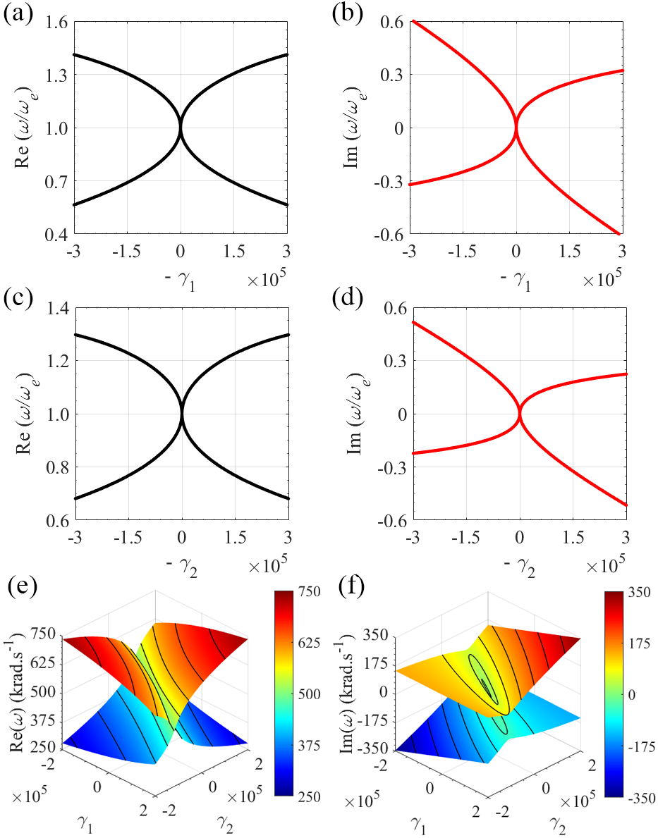
Figure 6: Case with negative value of the inductances on both resonators. Variation of (a) real and (b) imaginary parts of the angular eigenfrequencies to a resistor perturbation on the left resonator, i.e., when $-\gamma_{1}$ changes and $\gamma_{2}=0$. (c) and (d), as in (a) and (b), but the resistor perturbation is on the right resonator, i.e., $-\gamma_{2}$ changes and $\gamma_{1}=0$. Variation of (e) real and (f) imaginary parts of the angular eigenfrequencies to independent resistor perturbation on the both sides.

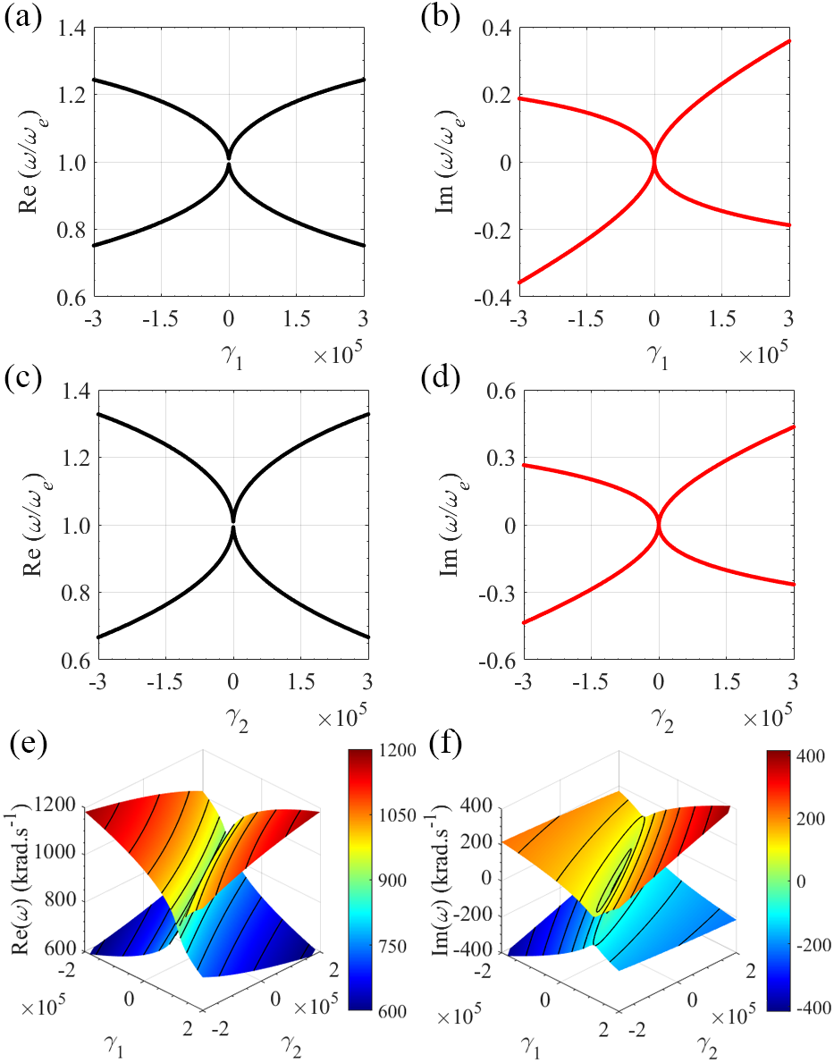
Figure 7: As in Fig. 6, except that these results pertain to the case where both capacitances are negative.

V-B RLC Resonators With Negative Capacitances $C_{1}$ and $C_{2}$

In the second case, we consider the negative value for capacitances. In Figs. 7(a) and (b), $\gamma_{1}$ is perturbed while we consider $\gamma_{2}=0$ and in Figs. 7(c), and (d), $\gamma_{2}$ is perturbed while $\gamma_{1}=0$. These figures show the real and imaginary parts of eigenfrequencies when each resistor is perturbed individually. We use the same values for the circuit components as used earlier in the lossless circuit shown in Subsection III-B, and the EPD angular frequency is obtained for these circuit parameters when $\gamma_{1}=\gamma_{2}=0$, which is the same EPD frequency of the lossless circuit. In Figs. 7(a)-(d), we observe the bifurcations of the real and imaginary parts of the eigenfrequencies, so the circuit is exhibits extreme sensitivity to resistance value variations in the vicinity of EPD. We show the real and imaginary parts of the eigenfrequencies by independently changing the resistances in both sides in 7(e)-(f). The black contour lines in these three-dimensional figures show constant real and imaginary parts of the eigenfrequencies. Angular eigenfrequencies are complex-valued when perturbing $\gamma_{1}$ and $\gamma_{2}$ away from $\gamma_{1}=\gamma_{2}=0$; hence the circuit gets unstable and it starts to oscillate at a fundamental frequency associated with the real part of the unstable angular eigenfrequency. In Figs. 7(a)-(f), both conditions $\gamma_{1}>0$ and $\gamma_{2}>0$ represent loss, whereas the conditions $\gamma_{1}<0$ and $\gamma_{2}<0$ represent gain in the circuit through a negative resistance.

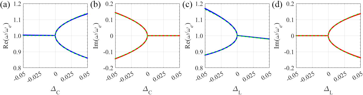
Figure 8: Sensitivity of (a) real and (b) imaginary parts of the eigenfrequencies to a capacitance perturbation (solid lines), $\Delta_{\mathrm{C}}=(C_{\mathrm{1}}-C_{\mathrm{1,\mathit{e}}})/C_{\mathrm{1,\mathit{e}}}$, while the inductances values on both sides are negative. Dashed lines show the perturbed eigenfrequencies according to the Puiseux expansion up to its first order. Sensitivity of (c) real and (d) imaginary parts of the eigenfrequencies to an inductance perturbation (solid lines), $\Delta_{\mathrm{L}}=(L_{\mathrm{1}}-L_{\mathrm{1,\mathit{e}}})/L_{\mathrm{1,\mathit{e}}}$, while the capacitances values on both sides are negative. Dashed lines show the perturbed eigenfrequencies according to Puiseux expansion up to its second order.

VI High-Sensitivity and Puiseux Fractional Power Series Expansion

Eigenfrequencies at EPDs are extremely sensitive to perturbations of the circuit elements, a property that is peculiar to the EPD condition. We study the circuit under EPD perturbation to investigate the circuit’s sensitivity near the EPD. We will demonstrate how small perturbations in a component’s value perturb the eigenfrequencies of the circuit. In order to do this analysis, the relative circuit perturbation $\Delta_{\mathrm{X}}$ is defined as

$$\Delta_{\mathrm{X}}=\frac{X-X_{\mathit{e}}}{X_{\mathit{e}}},$$ (15)

where $X$ is the perturbed parameter value, and $X_{\mathit{e}}$ is its unperturbed value that provides the EPD. The perturbation in $\Delta_{\mathrm{X}}$ value leads to a perturbed circuit matrix $\mathbf{\underline{M}}(\Delta_{\mathrm{X}})$. We demonstrate the extreme sensitivity to extrinsic perturbation by resorting to the general theory of EPD and utilizing the Puiseux fractional power series expansion [32]. Accordingly, when a small relative perturbation in component value $\Delta_{\mathrm{X}}$ is applied, the resulting two different eigenfrequencies $\omega_{\mathrm{\mathit{p}}}(\Delta_{\mathrm{X}})$, with $p=1,2$ are estimated using the convergent Puiseux series. Here we provide the first two terms to estimate the eigenfrequencies near an EPD, using the explicit formulas given in [38],

$$\omega_{p}(\Delta_{\mathrm{X}})\approx\omega_{\mathit{e}}+(-1)^{p}\alpha_{1}\sqrt{\Delta_{\mathrm{X}}}+\alpha_{2}\Delta_{\mathrm{X}},$$ (16)

$$\alpha_{1}=\left.\sqrt{-\frac{\frac{\partial H(\Delta_{\mathrm{X}},\omega)}{\partial\Delta_{\mathrm{X}}}}{\frac{1}{2!}\frac{\partial^{2}H(\Delta_{\mathrm{X}},\omega)}{\partial\omega^{2}}}}\right|_{\Delta_{\mathrm{X}}=0,\,\omega=\omega_{\mathrm{\mathit{e}}}},$$ (17)

$$\alpha_{2}=\left.-\frac{\alpha_{1}^{2}\frac{1}{3!}\frac{\partial^{3}H(\Delta_{\mathrm{X}},\omega)}{\partial\omega^{3}}+\frac{\partial^{2}H(\Delta_{\mathrm{X}},\omega)}{\partial\omega\partial\Delta_{\mathrm{X}}}}{\frac{\partial^{2}H(\Delta_{\mathrm{X}},\omega)}{\partial\omega^{2}}}\right|_{\Delta_{\mathrm{X}}=0,\,\omega=\omega_{\mathrm{\mathit{e}}}},$$ (18)

where $H(\Delta_{\mathrm{X}},\omega)=\mathrm{det}[\mathbf{\underline{M}}(\Delta_{\mathrm{X}})-j\omega\underline{\mathbf{I}}]$, and $\alpha_{1}$, and $\alpha_{2}$ are first- and second-order coefficients respectively. Eq. (16) indicates that for a tiny perturbation in component value $\Delta_{\mathrm{X}}\ll 1$ the eigenvalues change sharply from their original degenerate value due to the square root function, which is an essential characteristic of second-order EPD.

Typically, the inductor or capacitor changes in response to an external perturbation of the parameter of interest, leading to a shift in resonance frequency. We consider variations of $L_{\mathrm{1}}$, or $C_{\mathrm{1}}$, one at the time, and the calculated real and imaginary parts of the eigenfrequencies near the EPD is shown in Figs. 8. In the first case, the perturbation parameter is the capacitance, $\Delta_{\mathrm{C}}=(C_{\mathrm{1}}-C_{\mathrm{1,\mathit{e}}})/C_{\mathrm{1,\mathit{e}}}$, and a negative value for both inductances is assumed, so the first-order Puiseux expansion coefficient is calculated as $\alpha_{1}=3.228\times 10^{5}\>\mathrm{rad/s}$. To calculate the coefficients, we used the components value utilized in Subsection III-A. Figs. 8(a) and (b) exhibit the real and imaginary parts of the perturbed eigenfrequencies $\omega$ obtained from the eigenvalue problem after perturbing $\Delta_{\mathrm{C}}$. Furthermore, green dashed lines in these figures demonstrate such perturbed eigenfrequencies are well estimated with high accuracy by using the Puiseux expansion truncated at its first order. For a negative but small value of $\Delta_{\mathrm{C}}$, the imaginary part of the eigenfrequencies experiences a rapid change, and its real part remains constant. On the other hand, a very small positive value of $\Delta_{\mathrm{C}}$ causes a sharp change in the real part of the eigenfrequencies while its imaginary part remains unchanged.

In the second example, the inductance value in the left resonator is considered as a perturbed parameter, $\Delta_{\mathrm{L}}=(L_{\mathrm{1}}-L_{\mathrm{1,\mathit{e}}})/L_{\mathrm{1,\mathit{e}}}$, whereas capacitances values are both negative. By using Eqs. (17), and (18) and using the components value utilized in Subsection III-B, the coefficients of the Puiseux expansion are calculated as $\alpha_{1}=j5.548\times 10^{5}\>\mathrm{rad/s}$ and $\alpha_{2}=-3.960\times 10^{5}\>\mathrm{rad/s}$. The calculated results in Figs. 8(c), and (d) show the two branches (solid lines) of the exact perturbed eigenfrequencies evaluated from the eigenvalue problem when the external perturbation is applied to the circuit. This figure shows that the perturbed eigenfrequencies are estimated accurately by applying the Puiseux expansion truncated at its second order (dashed lines). For a tiny value of positive perturbation, the imaginary part of the eigenfrequencies undergoes sharp changes, while its real part remains approximately unchanged. However, a small negative perturbation in the inductance value rapidly changes the real part of the two eigenfrequencies away from the EPD eigenfrequency. The bifurcation in the diagram, described by a square root, is the most exceptional physical property associated with the EPD. It can be employed to devise ultra-sensitive sensors for various applications [39, 11, 40, 41].

VII Sensing Scenario for Liquid Content Measurement

In recent years various well-established techniques has been proposed to measure the liquid level such as light-reflection sensors [42], chirped fiber Bragg grating [43, 44], fiber optic sensors [45, 46, 47], ultrasonic Lamb waves [48], and capacitive sensors [49, 50, 51, 52]. The use of a capacitive sensor is a well-known method for liquid level measurement [53]. This kind of sensor has been proven to be stable, can be assembled using various materials, and can provide high resolution [54]. The principle of operation of capacitive sensors is that it converts a variation in position, or material characteristics, into measurable electrical signals [55]. Capacitive sensors are operated by changing any of the three main parameters: relative dielectric constant, area of capacitive plates, and distance between the plates. In conventional methods, a capacitive liquid level detector can sense the fluid level by measuring variations in capacitance made between two conducting plates embedded outside a non-conducting tank or immersed in the liquid [56, 53]. The same concept applies when the liquid occupies a varying volume percentage as a mixture’s component.

The following design will provide the schematic of a practical scenario to investigate the gyrator-based circuit application for physical parameter measurement. We provide the required setup and the measurement procedure to measure the liquid volume. Here, we use the following set of values for the components in the gyrator-based circuit $L_{1}=-4.7\mathrm{\>nH}$, $L_{2}=-4.7\mathrm{\>nH}$, $C_{2}=47\mathrm{\>pF}$, and $R_{g}=50\>\Omega$. Consider a cylindrical glass with top and bottom metal plates. This structure can serve as a variable capacitor in which the volume of filled liquid (or a percentage of a mixture) can change the total capacitance. A schematic structure for this scenario is illustrated in Fig. 9(a). The designed device includes the gyrator-based circuit (see Fig. 1) where the positive capacitor on the left side is the cylindrical container with height $d_{2}=3.0142\>\mathrm{cm}$, of which a height $d_{1}$ is filled with water and the area of metal plates are $A=100\>\mathrm{cm^{2}}$. Pure water is assumed to have a relative permittivity of $\varepsilon_{r}=78.7$ at $T=22.0^{\mathrm{o}}\>\mathrm{C}$, and we neglect losses in this simple case [57]. Two series variable capacitors model the structure, that the bottom one has a capacitance $C_{filled}=\varepsilon_{0}\varepsilon_{r}A/d_{1},$and the top one has a capacitance $C_{empty}=\varepsilon_{0}A/(d_{2}-d_{1})$. The total capacitance is $C_{total}=C_{filled}C_{empty}/(C_{filled}+C_{empty})$, which changes when varying the water level. By opening the top inlet, the height of water increases, so the capacitance value will be increased. On the contrary, the water’s height decreases when opening the bottom outlet, and the total capacitance value will be decreased. In summary, a level of water is related to the capacitance, and the perturbation in the value of capacitance will change a circuit’s eigenfrequencies. Using the explained steps in Section III and by solving the eigenvalue problem, the plot of resonance frequency versus water level percentage for this specific example is illustrated in Fig. 9(b) by the solid blue line. The measuring scheme is very sensitive near $0\%$ water content. The EPD can be designed for different water contents, so the frequency variation caused by changes in the water level around that mentioned level would be very sensitive. We now compare the sensitivity of the EPD-based scheme with that of a single LC resonator. We consider an LC resonator with the resonance frequency of $\omega_{0}=\omega_{e}$, i.e., coincident with one of the EPD systems. We assume that the sensing capacitor is the same as the one in Fig. 9, i.e., the same as that considered in the EPD system. The variation in the resonance frequency by perturbing the capacitance as described above, i.e., the level of water content, is shown in Fig. 9(b) by the red dashed line. It is clear that the EPD-based bifurcation in the dispersion diagram, characterized by a square root, dramatically enhances the circuit’s sensitivity compared to the sensitivity of the single LC resonator to the same capacitance perturbation.

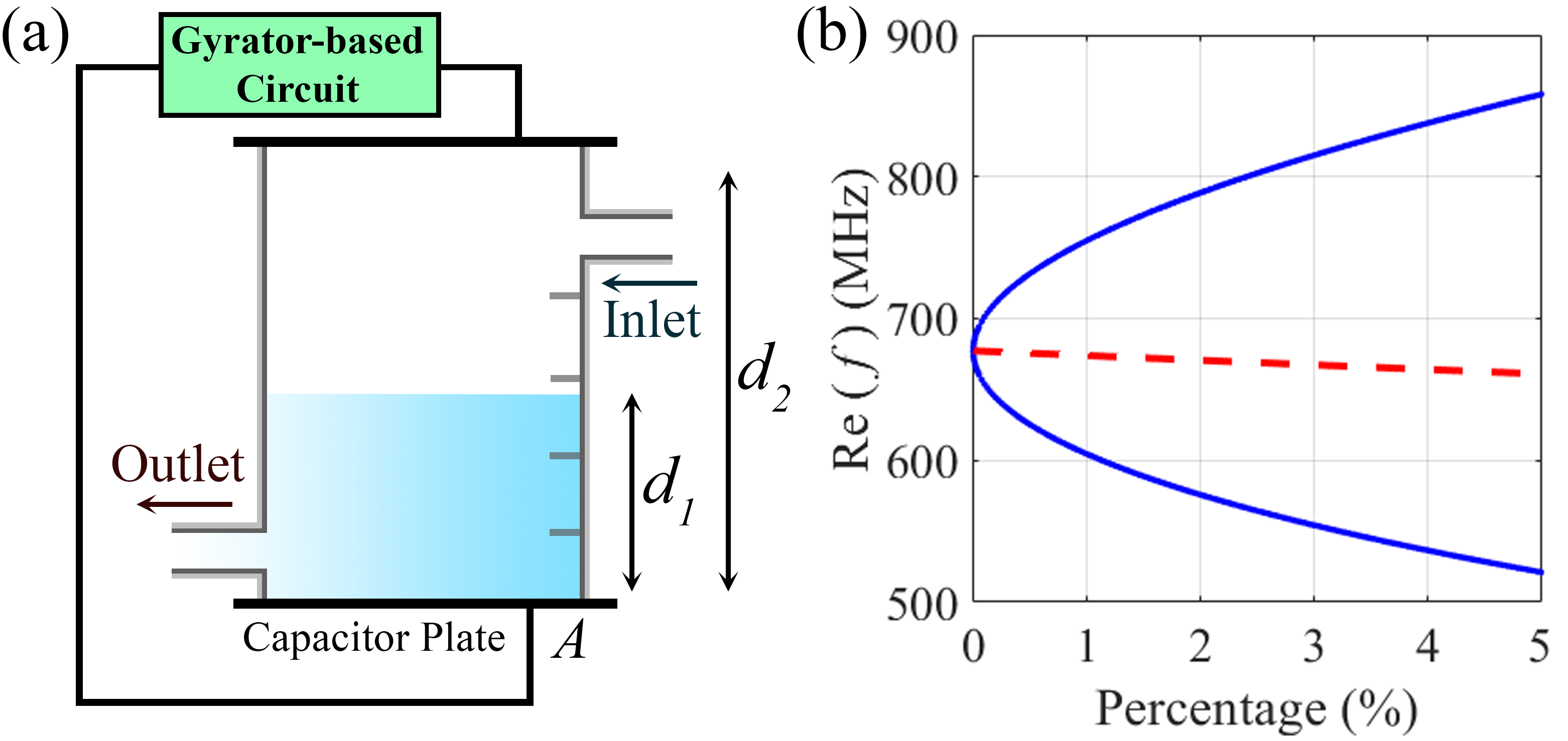
Figure 9: (a) Schematic illustration of a device for liquid level measurement. (b) The EPD is designed at a given level of water content ($0\%$ in the figure). The solid blue line in the plot shows the two resonance frequencies of the gyrator-based circuit versus water level variation with very high sensitivity near $0\%$. Also, the red dashed line shows the resonance frequency of a single resonator when the water content changes. The EPD-based circuit and the single LC resonator have the same resonance frequency at $0\%$. It is clear that the EPD-based circuit provides much higher sensitivity to the capacitance perturbation than the single LC resonator.

In the proposed scheme for liquid content measurement, we assumed that the gyrator-based circuit works in the stable region where eigenfrequencies were purely real. However, when considering the instabilities generated by losses, one eigenfrequency has a negative imaginary value, as explained in Section V. Consequently, the circuit starts having growing oscillations. The exponential growth rate can be controlled in two ways: either by stopping (switching off) the circuit to reach saturation or by letting it saturate. In this latter case, the gyrator-based circuit should be designed as a sensor that oscillates. The circuit can be used to sense physical or chemical parameters changes by measuring the oscillation frequency variations.

VIII Conclusions

The second-order EPD with real (degenerate) eigenfrequency in a gyrator-based circuit is achieved using two unstable series LC resonators coupled via an ideal gyrator. Both resonators have either negative capacitances or negative inductances. The resonance frequency of each resonator (when uncoupled) is purely imaginary, and we have demonstrated that the EPD frequency can be purely real. However, when losses are considered in the circuit, the system becomes unstable. We have focused on the physics of the EPD in this kind of gyrator-based circuit, looking at enhanced sensitivity when perturbing either the gyration resistance, a capacitance, or an inductance. In the potential application, the perturbation in the circuit can be estimated by measuring the shift of resonance frequencies. The presented results may have significant implications in sensing technology, security systems, particle monitoring, and motion sensors.

Acknowlegment

This material is based upon work supported by the National Science Foundation under Grant No. ECCS-1711975 and by AFOSR Grant No. FA9550-19-1-0103.

References

- [1] W. Heiss, “Repulsion of resonance states and exceptional points,” Physical Review E, vol. 61, no. 1, p. 929, 2000.
- [2] A. Figotin and I. Vitebskiy, “Oblique frozen modes in periodic layered media,” Physical Review E, vol. 68, no. 3, p. 036609, Sep 2003.
- [3] A. Figotin and I. Vitebskiy, “Gigantic transmission band-edge resonance in periodic stacks of anisotropic layers,” Physical review E, vol. 72, no. 3, p. 036619, 2005.
- [4] H. Ramezani, T. Kottos, V. Kovanis, and D. N. Christodoulides, “Exceptional-point dynamics in photonic honeycomb lattices with PT symmetry,” Physical Review A, vol. 85, no. 1, p. 013818, 2012.
- [5] M. V. Berry, “Physics of nonhermitian degeneracies,” Czechoslovak journal of physics, vol. 54, no. 10, pp. 1039–1047, Oct 2004.
- [6] C. M. Bender and S. Boettcher, “Real spectra in non-Hermitian Hamiltonians having PT symmetry,” Physical Review Letters, vol. 80, no. 24, pp. 2455–2464, Jun 1998.
- [7] H. Hodaei, M.-A. Miri, M. Heinrich, D. N. Christodoulides, and M. Khajavikhan, “Parity-time symmetric microring lasers,” Science, vol. 346, no. 6212, pp. 975–978, Nov 2014.
- [8] P.-Y. Chen, M. Sakhdari, M. Hajizadegan, Q. Cui, M. M.-C. Cheng, R. El-Ganainy, and A. Alu, “Generalized parity-time symmetry condition for enhanced sensor telemetry,” Nature Electronics, vol. 1, no. 5, pp. 297–304, May 2018.
- [9] T. Stehmann, W. Heiss, and F. Scholtz, “Observation of exceptional points in electronic circuits,” Journal of Physics A: Mathematical and General, vol. 37, no. 31, p. 7813, 2004.
- [10] J. Schindler, A. Li, M. C. Zheng, F. M. Ellis, and T. Kottos, “Experimental study of active LRC circuits with PT symmetries,” Physical Review A, vol. 84, no. 4, p. 040101, Oct 2011.
- [11] M. Sakhdari, M. Hajizadegan, Y. Li, M. M.-C. Cheng, J. C. Hung, and P.-Y. Chen, “Ultrasensitive, parity–time-symmetric wireless reactive and resistive sensors,” IEEE Sensors Journal, vol. 18, no. 23, pp. 9548–9555, 2018.
- [12] Y. J. Zhang, H. Kwon, M.-A. Miri, E. Kallos, H. Cano-Garcia, M. S. Tong, and A. Alu, “Noninvasive glucose sensor based on parity-time symmetry,” Physical Review Applied, vol. 11, no. 4, p. 044049, 2019.
- [13] J. Wiersig, “Enhancing the sensitivity of frequency and energy splitting detection by using exceptional points: application to microcavity sensors for single-particle detection,” Physical Review Letters, vol. 112, no. 20, p. 203901, 2014.
- [14] J. Wiersig, “Sensors operating at exceptional points: General theory,” Physical Review A, vol. 93, no. 3, p. 033809, Mar 2016.
- [15] J. Wiersig, “Robustness of exceptional-point-based sensors against parametric noise: the role of Hamiltonian and Liouvillian degeneracies,” Physical Review A, vol. 101, no. 5, p. 053846, 2020.
- [16] J. Wiersig, “Review of exceptional point-based sensors,” Photonics Research, vol. 8, no. 9, pp. 1457–1467, 2020.
- [17] J. Wiersig, “Prospects and fundamental limits in exceptional point-based sensing,” Nature communications, vol. 11, no. 1, pp. 1–3, 2020.
- [18] S. Gwak, H. Kim, H.-H. Yu, J. Ryu, C.-M. Kim, and C.-H. Yi, “Rayleigh scatterer-induced steady exceptional points of stable-island modes in a deformed optical microdisk,” Optics Letters, vol. 46, no. 12, pp. 2980–2983, 2021.
- [19] K. Rouhi, R. Marosi, T. Mealy, A. F. Abdelshafy, A. Figotin, and F. Capolino, “Exceptional degeneracies in traveling wave tubes with dispersive slow-wave structure including space-charge effect,” Applied Physics Letters, vol. 118, no. 26, p. 263506, 2021.
- [20] P. Djorwe, Y. Pennec, and B. Djafari-Rouhani, “Exceptional point enhances sensitivity of optomechanical mass sensors,” Physical Review Applied, vol. 12, no. 2, p. 024002, 2019.
- [21] Q. Wang and Y. Liu, “Review of optical fiber bending/curvature sensor,” Measurement, vol. 130, pp. 161–176, 2018.
- [22] B. D. Tellegen, “The gyrator, a new electric network element,” Philips Res. Rep, vol. 3, no. 2, pp. 81–101, 1948.
- [23] D. C. Hamill, “Lumped equivalent circuits of magnetic components: the gyrator-capacitor approach,” IEEE transactions on power electronics, vol. 8, no. 2, pp. 97–103, 1993.
- [24] D. Sheahan and H. Orchard, “Integratable gyrator using mos and bipolar transistors,” Electronics letters, vol. 2, no. 10, pp. 390–391, 1966.
- [25] T. Rao and R. Newcomb, “Direct-coupled gyrator suitable for integrated circuits and time variation,” Electronics Letters, vol. 2, no. 7, pp. 250–251, 1966.
- [26] A. Morse and L. Huelsman, “A gyrator realization using operational amplifiers,” IEEE Transactions on Circuit Theory, vol. 11, no. 2, pp. 277–278, 1964.
- [27] R. Riordan, “Simulated inductors using differential amplifiers,” Electronics Letters, vol. 3, no. 2, pp. 50–51, 1967.
- [28] A. Antoniou, “Gyrators using operational amplifiers,” Electronics Letters, vol. 3, no. 8, pp. 350–352, 1967.
- [29] A. Nikzamir, K. Rouhi, A. Figotin, and F. Capolino, “Demonstration of exceptional points of degeneracy in gyrator-based circuit for high-sensitivity applications,” arXiv preprint arXiv:2107.00639, 2021.
- [30] A. Figotin, “Synthesis of lossless electric circuits based on prescribed Jordan forms,” Journal of Mathematical Physics, vol. 61, no. 12, p. 122703, 2020.
- [31] A. Figotin, “Perturbations of circuit evolution matrices with Jordan blocks,” Journal of Mathematical Physics, vol. 62, no. 4, p. 042703, 2021.
- [32] T. Kato, Perturbation Theory for Linear Operators, 2nd ed. Springer-Verlag, Berlin Heidelberg, 1995, vol. 132.
- [33] M. Ehsani, I. Husain, and M. O. Bilgiç, “Power converters as natural gyrators,” IEEE Transactions on Circuits and Systems I: Fundamental Theory and Applications, vol. 40, no. 12, pp. 946–949, 1993.
- [34] B. Shenoi, “Practical realization of a gyrator circuit and rc-gyrator filters,” IEEE Transactions on Circuit Theory, vol. 12, no. 3, pp. 374–380, 1965.
- [35] W. D. Heiss, “Exceptional points of non-Hermitian operators,” Journal of Physics A: Mathematical and General, vol. 37, no. 6, pp. 2455–2464, Jan 2004.
- [36] H. Kazemi, M. Y. Nada, T. Mealy, A. F. Abdelshafy, and F. Capolino, “Exceptional points of degeneracy induced by linear time-periodic variation,” Physical Review Applied, vol. 11, no. 1, p. 014007, Jan 2019.
- [37] H. Kazemi, A. Hajiaghajani, M. Y. Nada, M. Dautta, M. Alshetaiwi, P. Tseng, and F. Capolino, “Ultra-sensitive radio frequency biosensor at an exceptional point of degeneracy induced by time modulation,” IEEE Sensors Journal, 2020.
- [38] A. Welters, “On explicit recursive formulas in the spectral perturbation analysis of a Jordan block,” SIAM Journal on Matrix Analysis and Applications, vol. 32, no. 1, pp. 1–22, jan 2011.
- [39] H. Hodaei, A. U. Hassan, S. Wittek, H. Garcia-Gracia, R. El-Ganainy, D. N. Christodoulides, and M. Khajavikhan, “Enhanced sensitivity at higher-order exceptional points,” Nature, vol. 548, no. 7666, pp. 187–191, aug 2017.
- [40] K. Rouhi, H. Kazemi, A. Figotin, and F. Capolino, “Exceptional points of degeneracy directly induced by space-time modulation of a single transmission line,” IEEE Antennas and Wireless Propagation Letters, pp. 1–1, 2020.
- [41] T. Li, W. Wang, and X. Yi, “Enhancing the sensitivity of optomechanical mass sensors with a laser in a squeezed state,” Physical Review A, vol. 104, no. 1, p. 013521, 2021.
- [42] R. Azzam, “Light-reflection liquid-level sensor,” IEEE Transactions on Instrumentation and Measurement, vol. 29, no. 2, pp. 113–115, 1980.
- [43] B. Yun, N. Chen, and Y. Cui, “Highly sensitive liquid-level sensor based on etched fiber Bragg grating,” IEEE photonics technology letters, vol. 19, no. 21, pp. 1747–1749, 2007.
- [44] E. Vorathin, Z. Hafizi, A. Aizzuddin, M. K. A. Zaini, and K. S. Lim, “A novel temperature-insensitive hydrostatic liquid-level sensor using chirped FBG,” IEEE Sensors Journal, vol. 19, no. 1, pp. 157–162, 2018.
- [45] S. Khaliq, S. W. James, and R. P. Tatam, “Fiber-optic liquid-level sensor using a long-period grating,” Optics letters, vol. 26, no. 16, pp. 1224–1226, 2001.
- [46] H. Golnabi, “Design and operation of a fiber optic sensor for liquid level detection,” Optics and Lasers in Engineering, vol. 41, no. 5, pp. 801–812, 2004.
- [47] X. Lin, L. Ren, Y. Xu, N. Chen, H. Ju, J. Liang, Z. He, E. Qu, B. Hu, and Y. Li, “Low-cost multipoint liquid-level sensor with plastic optical fiber,” IEEE Photonics Technology Letters, vol. 26, no. 16, pp. 1613–1616, 2014.
- [48] V. Sakharov, S. Kuznetsov, B. Zaitsev, I. Kuznetsova, and S. Joshi, “Liquid level sensor using ultrasonic Lamb waves,” Ultrasonics, vol. 41, no. 4, pp. 319–322, 2003.
- [49] F. N. Toth, G. C. Meijer, and M. van der Lee, “A planar capacitive precision gauge for liquid-level and leakage detection,” IEEE transactions on Instrumentation and Measurement, vol. 46, no. 2, pp. 644–646, 1997.
- [50] H. Canbolat, “A novel level measurement technique using three capacitive sensors for liquids,” IEEE transactions on Instrumentation and Measurement, vol. 58, no. 10, pp. 3762–3768, 2009.
- [51] K. Chetpattananondh, T. Tapoanoi, P. Phukpattaranont, and N. Jindapetch, “A self-calibration water level measurement using an interdigital capacitive sensor,” Sensors and Actuators A: Physical, vol. 209, pp. 175–182, 2014.
- [52] J. R. Hanni and S. K. Venkata, “A novel helical electrode type capacitance level sensor for liquid level measurement,” Sensors and Actuators A: Physical, vol. 315, p. 112283, 2020.
- [53] B. Kumar, G. Rajita, and N. Mandal, “A review on capacitive-type sensor for measurement of height of liquid level,” Measurement and control, vol. 47, no. 7, pp. 219–224, 2014.
- [54] K. Loizou and E. Koutroulis, “Water level sensing: State of the art review and performance evaluation of a low-cost measurement system,” Measurement, vol. 89, pp. 204–214, 2016.
- [55] S. C. Bera, J. K. Ray, and S. Chattopadhyay, “A low-cost noncontact capacitance-type level transducer for a conducting liquid,” IEEE Transactions on Instrumentation and Measurement, vol. 55, no. 3, pp. 778–786, 2006.
- [56] E. Terzic, J. Terzic, R. Nagarajah, and M. Alamgir, A neural network approach to fluid quantity measurement in dynamic environments. Springer Science & Business Media, 2012.
- [57] N. S. Midi, K. Sasaki, R.-i. Ohyama, and N. Shinyashiki, “Broadband complex dielectric constants of water and sodium chloride aqueous solutions with different DC conductivities,” IEEJ Transactions on Electrical and Electronic Engineering, vol. 9, no. 1, pp. 8–12, 2014.