Gell-Mann-Low criticality in neural networks

Abstract

Criticality is deeply related to optimal computational capacity. The lack of a renormalized theory of critical brain dynamics, however, so far limits insights into this form of biological information processing to mean-field results. These methods neglect a key feature of critical systems: the interaction between degrees of freedom across all length scales, which allows for complex nonlinear computation. We present a renormalized theory of a prototypical neural field theory, the stochastic Wilson-Cowan equation. We compute the flow of couplings, which parameterize interactions on increasing length scales. Despite similarities with the Kardar-Parisi-Zhang model, the theory is of a Gell-Mann-Low type, the archetypal form of a renormalizable quantum field theory. Here, nonlinear couplings vanish, flowing towards the Gaussian fixed point, but logarithmically slowly, thus remaining effective on most scales. We show this critical structure of interactions to implement a desirable trade-off between linearity, optimal for information storage, and nonlinearity, required for computation.

Criticality and information processing are deeply related: Statistical descriptions of the hardest-to-solve combinatorial optimization problems, for example, are right at the edge of a phase transition (Cheeseman et al., 1991; Saitta et al., 2011). Also brain activity shows criticality (Beggs and Plenz, 2003; Chialvo, 2010), which may optimize the network’s computational properties. Among these, long spatio-temporal correlations support information storage and transmission, while rich collective and nonlinear dynamics allow degrees of freedom to cooperatively perform complex signal transformations (Langton, 1990).

A multitude of critical processes could lie behind critical brain dynamics. Thanks to the universality paradigm of statistical physics, however, their macroscopic behavior is organized into few classes, distinguished by only generic properties, like the system’s dimension, the nature of the degrees of freedom, as well as symmetries and conservation laws (Hohenberg and Halperin, 1977; Taeuber, 2014). Identifying the universality classes implemented by neural networks and finding their distinctive features is key to understanding if and how the brain exploits criticality to perform computation.

Theoretical analysis of critical brain dynamics is, however, so far restricted to mean-field methods. These partly explain why memory, dynamic range and signal separation are optimal at a critical point (Bertschinger and Natschläger, 2004; Bertschinger et al., 2005; Kinouchi and Copelli, 2006). Still, a fundamental aspect of critical computation is inaccessible to these methods: the nonlinear interaction between degrees of freedom across all length scales. By approximating fluctuations as Gaussian, mean-field theory can study only the linear response of individual modes to stimuli. But a single, uncoupled mode can solve only simple computational tasks. In fact, this approximation only holds if nonlinear interactions, albeit necessary for computation, are irrelevant on macroscopic scales. Thus, mean-field criticality is a special case, in fact the simplest but also the most restricted kind of criticality the brain could possibly implement. Uncovering different kinds of criticality requires more sophisticated methods.

In this letter we analyze criticality in the stochastic Wilson-Cowan rate model, a prototypical model of brain dynamics (Wilson and Cowan, 1972, 1973; Destexhe and Sejnowski, 2009). We use the non-equilibrium Wilsonian renormalization group to go beyond mean-field analysis (Hohenberg and Halperin, 1977; Taeuber, 2014). This technique tracks the flow of effective nonlinear couplings as one describes the system on gradually increasing length scales. This exposes the type of criticality featured by the system and its relevance for computation. The model is studied under a continuous stream of external inputs, as typical for interconnected brain areas (Schüz and Braitenberg, 2002; Destexhe et al., 2003). While critical activity in networks driven by sparse inputs is well described by branching processes (Beggs and Plenz, 2003; Haldeman and Beggs, 2005) belonging to the universality class of mean-field directed percolation (Henkel et al., 2008), it is still unclear whether constantly driven brain networks are able to support criticality at all (Fosque et al., 2021).

We find the Wilson-Cowan model can indeed be critical in this regime. The derived long-range description is very similar to that of the Kardar-Parisi-Zhang model (Kardar et al., 1986). But while the latter features a strong coupling fixed point, we find a completely different form of criticality: It is of the Gell-Mann-Low type, the archetypal criticality underlying renormalizability of quantum field theories (Gell-Mann and Low, 1954)(Wilson, 1975, Sec. V). This type of criticality occurs at the upper critical dimension, at which mean-field theory looses validity. We determine this to be $d=2$, in agreement with the planar organization of cortical networks. Nonlinear couplings decrease only logarithmically slowly, thus remaining effective on practically all length scales. This property implements a desirable balance between a linear behavior and a nonlinear one; the model optimally remembers signals presented in the past, due to its nearly linear dynamics, and at the same time can perform nonlinear classification.

Focusing on the key ingredients of neural networks, that are nonlinear dynamics of their constituents, noisy drive, and spatially localized nonlinear coupling, we consider a neural field following the well-known Wilson-Cowan equation

$$\tau\frac{dh}{dt}=-l\left(h\right)+w\ast f\left(h\right)+\sqrt{\tau}\,I\,,$$ (1)

where $h\left(x,t\right)$ is a neural activity field on the space $x\in\mathbb{R}^{d}$ that evolves in time $t$ on the characteristic time-scale $\tau$. The function $l$ describes intrinsic local dynamics, and $f$ is a nonlinear gain function. The connectivity kernel $w\left(x-x^{\prime}\right)$ weighs the input from the neural state at position $x^{\prime}$ to that at position $x$, and $\ast$ is the spatial convolution. Following a common approach (Ermentrout, 1998), the connectivity $w$ is the sum of two Gaussians with widths $\sigma_{\pm}$ and amplitudes $w_{\pm}$, with $\text{sign}\left(w_{\pm}\right)=\pm 1$, representing excitatory and inhibitory connections. External input from remote brain areas driving the local activity is, for simplicity, modeled as Gaussian white noise with statistics $\langle I\left(x,t\right)\rangle=\mu$ and $\langle I\left(x,t\right)I\left(x^{\prime},t^{\prime}\right)\rangle=D\delta\left(x-x^{\prime}\right)\,\delta\left(t-t^{\prime}\right)$. A microscopic length $a$ characterizes the spatial resolution of the model, thus Eq. (1) is defined on a square lattice with $N^{d}$ sites and spacing $a$, eventually taking the limit $N\to\infty$. Equivalently, momenta are restricted to $\left|k\right|<\Lambda\coloneqq\pi/a$.

The computational properties of the model are later tested in a reservoir computing setting (Lukoševičius and Jaeger, 2009): A linear readout is trained to extract a desired input-output mapping from the neural activity (Fig. 1(a)). Nonlinear interactions are fundamental to achieve complex mappings. We thus want to go beyond mean-field methods and instead track the relevance of nonlinear interactions on gradually increasing length scales.

We make explicit all nonlinear terms in Eq. (1) by Taylor expanding $f\left(x\right)=\sum_{n}f_{n}x^{n}$ and likewise $l$. Also, the momentum dependence of the Fourier transformed coupling kernel $\hat{w}\left(k\right)=\sum_{\pm}w_{\pm}\left(1-\frac{1}{2}\sigma_{\pm}^{2}k^{2}+\mathit{\mathcal{O}}\left(k^{4}\right)\right)$ is kept up to second order, enough to expose those terms that characterize the system on a mesoscopic length-scale. We thus obtain, in the spatial domain,

$$\tau\frac{dh}{dt}=\sum_{n=1}^{\infty}\left(-m_{n}+g_{n}\Delta+\mathcal{O}\left(\Delta^{2}\right)\right)\,h^{n}+I\,,$$ (2)

where $\Delta$ is the Laplace operator and $\mathit{\mathcal{O}}\left(\Delta^{2}\right)$ denotes all terms proportional to spatial differential operators of order $\geq 4$. Couplings are conveniently renamed $m_{n}\coloneqq l_{n}-f_{n}\sum_{\pm}w_{\pm}$, characterizing the local dynamics, and $g_{n}\coloneqq\frac{1}{2}f_{n}\sum_{\pm}\sigma_{\pm}^{2}w_{\pm}$, quantifying the interaction across space points. Notice $\mu$, $l_{0}$ and $f_{0}$, corresponding to a constant input causing $\langle h\rangle\neq 0$, are without loss of generality set to zero (see Supplemental Material).

Temporarily neglecting nonlinearities ($g_{n}$, $m_{n}=0$ $\forall n>1$), the mass term $m_{1}$ plays the role of a lower momentum cut-off (Wilson, 1975). This defines the system’s spatial ($\propto m_{1}^{-\frac{1}{2}}$) and temporal ($\propto m_{1}^{-1}$) correlation lengths, both diverging as $m_{1}\to 0$. Thus $m_{1}=0$ identifies a critical point of the linear model. To include the effect of nonlinearities close to this point, standard expansion methods fail: perturbative corrections diverge due to statistical fluctuations interacting on an infinite range of length scales (Wilson, 1975).

To tackle this issue, the renormalization group (RG) (Wilson, 1975; Hohenberg and Halperin, 1977; Taeuber, 2014) performs the integration of fluctuations gradually over momentum scales $\Lambda/\ell<\left|k\right|<\Lambda$; progressively increasing the flow parameter $\ell\in[1,\infty)$, we obtain a series of effective field theories, each describing only degrees of freedom on larger length scales, with $k<\Lambda/\ell$. Such theories are defined on the rescaled quantities $k_{\ell}\coloneqq\ell k$, $t_{\ell}\coloneqq\ell^{-z}t$, $\hat{h}_{\ell}\left(k_{\ell},t_{\ell}\right)\coloneqq\ell^{-\zeta}\hat{h}\left(k,t\right)$ and $\hat{I}_{\ell}\left(k_{\ell},t_{\ell}\right)\coloneqq\ell^{\chi}\hat{I}\left(k,t\right)$. Rescaling makes all effective field theories look formally equivalent to Eq. (2), differing only by the values of the couplings $m_{n}\left(\ell\right)$ and $g_{n}\left(\ell\right)$, which become $\ell$-dependent. This dependence accounts for two effects: The interaction with the integrated out degrees of freedom and the rescaling. The couplings’ flow with $\ell$ therefore characterizes nonlinear interactions on different length scales and, thus, the type of critical behavior featured by the system. For example, the flow running into a fixed point is a characteristic of critical systems and determines their typical scale invariance.

We begin with analyzing the coupling’s flow due to rescaling alone. This corresponds to standard dimensional analysis and the mean-field approach, neglecting the contribution of fluctuations. As typical brain networks have a planar organization, we are ultimately interested in the case $d=2$. We choose $z=2,$ $\zeta=\frac{d+2}{2},$ and $\chi=\frac{d-2}{2}$ so that $g_{1}$, $\tau$, and the input variance $D$ are at a fixed point (i.e. do not rescale). With this choice, for $d\geq 2$ all couplings not appearing explicitly in Eq. (2) rapidly flow to $0$ with some negative power of $\ell$. These couplings are termed irrelevant and can be neglected as the effective theory’s reference scale $\ell$ is increased. The couplings $m_{n}\left(\ell\right)=\ell^{2-\left(n-1\right)\frac{d-2}{2}}m_{n}\left(1\right)$ diverge at $d=2$ as $\sim\ell^{2}$. They are termed relevant, meaning they must be fine-tuned to $0$ to be at a fixed point. This fine-tuning here implies balance of inhibitory and excitatory inputs (see Supplemental Material), often observed in brain networks as a necessary condition for criticality (Shew et al., 2009). The couplings $g_{n}\left(\ell\right)=\ell^{-\left(n-1\right)\frac{d-2}{2}}g_{n}\left(1\right)$ vanish for $d>2$, $\forall n\geq 2$. For these spatial dimensions, mean-field theory is usually accurate: all nonlinear terms in Eq. (2) are negligible at large scales, thus fluctuations have almost no interactions and can be neglected. Conversely, dimensional analysis predicts $d=2$ as the upper critical dimension at which the $g_{n}$ do not scale and are thus termed marginal: their flow is driven by fluctuations alone and thus must be investigated with more sophisticated methods, like the RG.

The mean-field analysis above allows us to determine the form of the effective theory describing the critical system at a mesoscopic scale, where irrelevant couplings are negligible

$$\tau\frac{dh}{dt}=\Delta\left(g_{1}h+g_{2}h^{2}+g_{3}h^{3}\right)+I\,.$$ (3)

Notice that, at such scales, the field $h$ describes neural populations exchanging activity with nearest neighbors via a diffusive process, as expressed by the Laplace operator $\Delta$ (di Santo et al., 2018). Among the marginal couplings $g_{n}$, we keep only the first $n\leq n_{0}=3$. We can assume neural activity to mainly explore a limited range of the gain function (Ostojic and Brunel, 2011; Roxin et al., 2011), which can therefore be locally approximated with a polynomial. We choose $n_{0}=3$ to keep a minimal approach ($n_{0}=2$ cannot be chosen, as Eq. (3) would be unstable). Equation (3) was proposed as an alternative to the Kardar-Parisi-Zhang (KPZ) model (Pavlik, 1994; Antonov and Vasiliev, 1995), both describing the dynamic growth of interfaces. The original KPZ model (Kardar et al., 1986) defines the KPZ universality class, where the interaction flows into a strong-coupling fixed point. Despite the similarities, we show Eq. (3) to exhibit a radically different type of critical behavior.

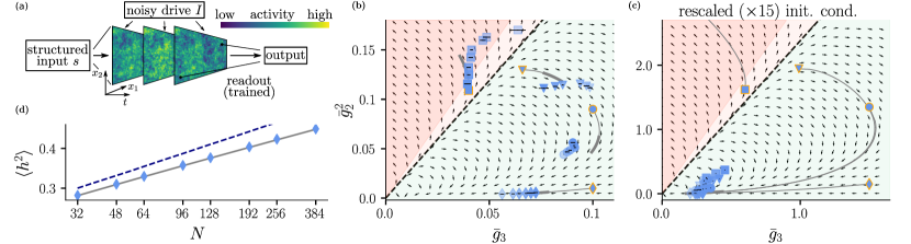
Figure 1: Phase diagram and flow of couplings. (a) Scheme of the model. (b) and (c): Direction of flow (arrows) in the $\bar{g}_{3}-\bar{g}_{2}^{2}$ plane, as defined by Eq. (5) and Eq. (6). The transition line (black, dashed) separates the plane in a converging (green) and diverging region (red). Region of non-physical bi-stable regime in darker red (see Supplemental Material). Blue markers represent the measured flow of couplings at $\ell=\frac{N}{2}$, with $N\in\left\{32,48,64,96,128,192\right\}$ (dark to light shading; squares in (b) also include $N=256,384$) for different initial conditions (yellow edge). Gray solid lines (thicker within the range of simulated $\ell$) represent the corresponding predicted flow. (d): Measured variance (blue diamonds) as a function of $N$ for $\bar{g}_{3}=0.1$ and $\bar{g}_{2}^{2}=0.01$ ($\bar{g}_{2}^{2}\ll\bar{g}_{3}$ regime), compared against the linear case (dashed, dark blue line) and prediction (gray, solid line).

We start from Eq. (3) to compute the fluctuation-driven part of the couplings’ flow. This is conveniently done by mapping Eq. (3) to a field theory by means of the Martin-Siggia-Rose-de Dominicis-Janssen formalism (Martin et al., 1973; De Dominicis, 1976; Hertz et al., 2017; Helias and Dahmen, 2020). Flow equations are then computed to one-loop order with Feynman diagram techniques, within the framework of the infinitesimal momentum shell Wilsonian RG for non-equilibrium systems (Hohenberg and Halperin, 1977) (details in Supplemental Material). Notice only $g_{2}$ and $g_{3}$ are meaningful parameters, as one can rewrite Eq. (3) in dimensionless form by setting $\tau,\,g_{1},\,D$ and $a$ to unity and renaming $\bar{g}_{n}\coloneqq\left(D/g_{1}\right)^{\frac{n-1}{2}}\frac{g_{n}}{g_{1}}$. We use this convention for the remainder of this letter. Defining $s\coloneqq\left(2\pi\right)^{-1}\ln\left(\ell\right)$, the differential flow equations take the form

$$\frac{1}{g_{1}}\frac{dg_{1}}{ds}=\frac{3}{2}\bar{g}_{3}-\bar{g}_{2}^{2},$$ (4)

$$\frac{d\bar{g}_{2}^{2}}{ds}=-\frac{27}{2}\bar{g}_{3}\bar{g}_{2}^{2}+7\bar{g}_{2}^{4},$$ (5)

$$\frac{d\bar{g}_{3}}{ds}=-\frac{15}{2}\bar{g}_{3}^{2}+14\bar{g}_{3}\bar{g}_{2}^{2}-4\bar{g}_{2}^{4}\,,$$ (6)

showing that $\bar{g}_{2}$ and $\bar{g}_{3}$ alone drive the flow. The Laplace operator in front of the nonlinear terms in Eq. (3) protects $D$, $\tau$ and $m_{n}$ from fluctuation corrections (see Supplemental Material), so their flow is completely determined by the mean-field analysis above. Fig. 1(b) shows the flow vector field in the $\bar{g}_{3}-\bar{g}_{2}^{2}$ plane. A line $\frac{\bar{g}_{2}^{2}}{\bar{g}_{3}}=\frac{7+\sqrt{145}}{8}$ determines a transition between a diverging and converging behavior.

Below the transition line, the couplings vanish, flowing into the Gaussian fixed point $(\bar{g}_{2}=\bar{g}_{3}=0$). Differently than in a mean-field scenario, however, the flow is logarithmically slow in $\ell$, a characteristic of marginal couplings at the upper critical dimension. This means interactions are effectively present on a wide range of length scales. Finite-size systems typically do not even reach the extent beyond which interactions become truly negligible. This is known as Gell-Mann-Low criticality, the archetypal behavior underlying renormalizability of quantum field theories, such as Quantum Electrodynamics (QED) (Gell-Mann and Low, 1954)(Wilson, 1975, Sec. V). Here one observes nonlinearities that shape non-trivial electro-magnetic interactions on a wide range of scales. A difference to a prototypical Gell-Mann-Low theory, however, is that the flow is driven by the pair of marginal couplings $(\bar{g}_{2},\bar{g}_{3})$, rather than by a single coupling, which for QED is the charge. At large scales, the power law scaling exponents $z,\,\zeta$, and $\chi$ maintain their mean-field values, since interactions eventually vanish. However, logarithmic corrections must be included due to the slowness of the flow. One example of this effect can be seen in the scaling of the variance $\big{\langle}h^{2}\big{\rangle}$ as a function of $N$ shown in Fig. 1(d). These logarithmic corrections may also be mistaken as different power law exponents, which depend on the system’s dynamical state, rather than being universal. Thus they can lead to small, state-dependent shifts in measured scaling exponents with respect to their mean-field value (see Supplemental Material).

As previously noted by (Antonov and Vasiliev, 1995), the infinite number of marginal couplings $g_{n}$ in principle allows for the existence of an infinite number of fixed points. Determining analytically whether these are attractive, though, has never been done due to the technical difficulty of the task. In neglecting $g_{n}$, $\forall n>3$, we are implicitly assuming the Gaussian fixed point is stable, with a sufficiently large basin of attraction to attract the flow from any initial $g_{n}$. We therefore test the validity of the flow equations numerically, by integrating Eq. (3) with the Euler-Maruyama algorithm (Kloeden and Platen, 1992)(additional details in Supplemental Material). Measurements are restricted to $\bar{g}_{2}^{2}<3\bar{g}_{3}$ (Fig. 1(b)), due to the occurrence of an unphysical bi-stable regime above such boundary (Supplemental Material).

We simulate systems of increasing size $N$, which limits the extent of correlations. By measuring correlation functions of the neural field $h$, we extract the value of the flown couplings at different length scales $\ell=\frac{N}{2}$ and initial conditions, shown in Fig. 1(b). Below the transition line, we observe good qualitative agreement between the measured and predicted flow. Quantitative departures from predictions are expected, given the approximation made to one-loop order in fluctuations and to third order in the expansion of $f$. This approximation is good enough, given our goal to qualitatively confirm the running of the flow towards the Gaussian fixed point. Higher orders could be easily included, if needed, at the relatively low cost of computing more Feynman diagrams.

Above the transition line instead, our approximation leads to a divergence of the flow. This could signal the presence of a strong coupling fixed point, into which the flow eventually runs. This occurs, for example, in the KPZ model for $d\geq 3$, where an analogous transition point exists (Fogedby and Ren, 2009). Differently, however, our measurements in Fig. 1(b) suggest the flow still heads towards the Gaussian fixed point, making a u-turn similar to when starting close and below the transition line. This is confirmed in Fig. 1(c), showing the flow for larger initial values of the couplings. The flow is then subject to a stronger drive in its initial transient, thus spanning a longer trajectory within the same range of $\ell$. These measurements thus suggest that, regardless of the initial condition, after an initial transient the flow always runs into the $\bar{g}_{3}\gg\bar{g}_{2}^{2}$ region, heading towards the Gaussian fixed point. Luckily, this region is where the flow equations in the given approximation yield reliable quantitative predictions. This is exemplified by the measured neural field variance $\big{\langle}h^{2}\big{\rangle}$ as a function of $N$ being well predicted by theory (Fig. 1(d)). In the limit $N\to\infty$, we predict $\big{\langle}h^{2}\big{\rangle}\sim\left(4\pi g_{1}\left(\ell\right)\right)^{-1}\ln\left(\frac{N}{2}\right)$, with $\ell\overset{!}{=}\frac{N}{2}$ (see Supplemental Material). The $\ell$-dependence of $g_{1}$ shows a logarithmic correction with respect to the linear case, in which $g_{1}\left(\ell\right)=1$ $\forall\ell$.

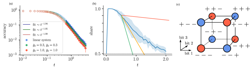
Figure 2: Examples of computation. (a) Memory: reconstruction accuracy over time of a Gaussian input for different strengths of the nonlinearties (legend). Values range from $0$ (complete forgetting) to $1$ (perfect reconstruction). (b) Classification: Share of correctly classified $3$-bit strings (blue line) and standard deviation across repeated trainings (blue area). Other curves decay with the time-scale of the slowest (red), middle (orange) and fastest (green) modes available at readout. (c) Spatial position of the $3$-bit strings, colored by their parity.

We have so far demonstrated that the system showcases criticality of the Gell-Mann-Low kind. The question remains on why, among types of criticality, this one would be especially beneficial for computation. Criticality optimizes desirable computational properties; still, these may strive for a balance between a linear behavior, optimal for storage and transmission of information, and a nonlinear one, necessary for computation. The Gell-Mann-Low criticality implements such a balance by sitting in-between a mean-field and strong coupling fixed point scenario. We exemplify this by training the system Eq. (3) to solve example tasks by what is known as reservoir computing (Fig. 1(a)) (Lukoševičius and Jaeger, 2009): A structured input $s$ is fed at some time $t_{\mathit{in}}$ in the form of a perturbation $h\left(x,t_{\mathrm{in}}\right)+s\left(x\right)$. At a later time $t_{\mathrm{out}}$, a linear readout $\sum_{x}W\left(x\right)h\left(x,t_{\mathrm{out}}\right)$ is taken and the parameters $W\left(x\right)$ are trained with gradient descent (task-specific details in Supplemental Material).

We first focus on memory; for concreteness, consider the Fischer memory curve (Ganguli et al., 2008). In the linear case, it is expected to be optimal, and to decay with time as $t^{-2}$. Being a global feature, involving the system as a whole on long time scales, it benefits from the system’s closeness to linear dynamics. Indeed, since nonlinearities vanish on a global length scale, as opposed to a strong coupling fixed point scenario, they do not worsen the power law decay found in the optimal linear case; rather they cause only small logarithmic corrections. Inspired by these theoretical grounds, we train $N^{2}$ linear readouts to reconstruct a Gaussian-shaped input at some time $t$ after injection, recording the reconstruction accuracy (Fig. 2(a)). As expected, increasing the strength of nonlinearities, the accuracy’s power law exponent does not deviate appreciably from the linear case: performance is only worsened by a constant shift in double logarithmic scale.

In contrast to a strict mean-field scenario, nonlinearities are, however, still relevant on most length scales other than the very macroscopic ones, thus allowing the system’s degrees of freedom to interact and to collectively perform computation. We exemplify this by training two linear readouts to correctly classify the parity of $3$-bit strings. The task is not linearly separable: no plane can correctly separate the strings in the two categories (Fig. 2(c)). Nonlinear dynamics are necessary to expand the input’s dimensionality, thus making linear separation possible. The input string’s $n$-th bit is encoded by the sign of a perturbation of the Fourier mode of momentum $k_{n}=\left(\pi-n\,4\pi/N\right)\hat{e}_{1}$, right below the high momentum cut-off $\pi$. The linear readout is taken on a low-pass filtered $h$, restricted to momenta $<\left|k_{3}\right|$. Thus nonlinear dynamics are further necessary to transfer information from the input to the readout modes. Fig. 2(b) indeed shows successful training. Performance decays on a time scale between the characteristic scales of the slowest and fastest modes, suggesting their collective interaction to be employed to perform the task. The modes’ response shown in the Supplemental Material further imply this, see Fig. LABEL:fig:k_modes.

In conclusion, we furnish the tools, a renormalized theory of neural network dynamics, to uncover the structure of nonlinear interactions across scales, so far inaccessible by mean-field methods. This framework opens the door to explore many other forms of criticality, beyond mean-field, that neural networks might implement, and to quantitatively address nonlinear signal transformations at a dynamical critical point. Applying the methods to the stochastic Wilson-Cowan model, we find a new form of criticality, which is robust to the biologically plausible external drive. At the relevant dimension $d=2$, critical behavior ceases to be mean-field, being instead of the Gell-Mann-Low kind. Most notably, nonlinear couplings, fundamental for computation, have a logarithmically slow, rather than power-law vanishing flow. We argue that this supports a computationally optimal balance between linear and nonlinear dynamics. The RG methodology and the concept of Gell-Mann-Low criticality are generally applicable to any stochastic dynamical system. We thus foresee applications to computation-oriented, possibly more complex models, both biological and artificial. For example, Gell-Mann-Low criticality could naturally account for the variability in critical exponents observed in the context of neural avalanches (Fontenele et al., 2019; Carvalho et al., 2021). The link between neural field theory, the KPZ model central to non-equilibrium statistical physics, and quantum field theory presents a stepping stone to transfer expertise from these fields, where RG methods are widely used.