Posterior predictive model assessment using formal methods in a spatio-temporal model

Abstract

We propose an interdisciplinary framework, Bayesian formal predictive model assessment. It combines Bayesian predictive inference, a well established tool in statistics, with formal verification methods rooting in the computer science community.

Bayesian predictive inference allows for coherently incorporating uncertainty about unknown quantities by making use of methods or models that produce predictive distributions, which in turn inform decision problems. By formalizing these problems and the corresponding properties, we can use spatio-temporal reach and escape logic to formulate and probabilistically assess their satisfaction. This way, competing models can directly be compared based on their ability to predict the property satisfaction a posteriori.

The approach is illustrated on an urban mobility application, where the crowdedness in the center of Milan is proxied by aggregated mobile phone traffic data. We specify several desirable spatio-temporal properties related to city crowdedness such as a fault-tolerant network or the reachability of hospitals. After verifying these properties on draws from the posterior predictive distributions, we compare several spatio-temporal Bayesian models based on their overall and property-based predictive performance.

1 Introduction

In this paper, we combine Bayesian inference with formal verification methods widely employed in the computer science literature to specify, verify and evaluate requirements or properties that a spatio-temporal measure of population crowdedness shall satisfy for different decision problems. This interdisciplinary framework provides a unifying approach to the modeling and statistical analysis of data that coherently accounts for uncertainty through the Bayesian paradigm and can be directly employed for decision-making by incorporating application- and decision-specific requirements into the model assessment procedure.

Bayesian predictive inference allows to coherently account for uncertainty about an unknown or future value of a random variable being modeled by providing the entire posterior predictive distribution. Posterior predictive model evaluation and checking (Rubin, 1984) is then employed to check the predictive performance of a Bayesian model on unseen data by qualitatively and quantitatively assessing how well the posterior predictive distributions produced by a model reflect existing data. Formally, from a decision theoretic point of view, the predictive performance of a model is typically defined in terms of a utility or scoring function that measures the quality of the predictive distribution of candidate models (Bernardo and Smith, 1994). Especially when a temporal component is present both in the data and in the modeling framework, the posterior predictive distribution for different time intervals will inform a series of decision problems. Clearly, in the decision-making process, these future values are unknown ex-ante but will be observed ex-post, i.e., after the decision has been taken, so competing models can be compared based on evaluating the out-of-sample posterior predictive distribution given the future observed values. These predictive distributions can be obtained either in an exact fashion, by employing a (time-series) cross-validation where the model is re-estimated as new observations come in, or in an approximate fashion (see e.g., Vehtari et al., 2017; Bürkner et al., 2020). A large body of literature has been concerned with how models should be evaluated and compared based on these predictive distributions, with various versions of predictive density scores being proposed (see, e.g. Corradi and Swanson, 2006; Geweke and Amisano, 2010; Frazier et al., 2021).

Ideally, the score functions or rules employed in the model assessment should be specifically tailored for the application at hand, and the model assessment and comparison should take into account the process through which the prediction of future data with the model enters a decision. However, such approaches are rather limited in the literature, where commonly used measures based on, e.g., logarithmic scores are chosen for their desirable mathematical properties. Indeed, in most applications predictions obtained from a (Bayesian) model are often not directly translated into a decision but rather transformed, compressed, and combined with further rules or requirements relevant for the decision problem at hand. As a simple example, consider an algorithmic trading scheme using a predictive model for stock returns, which will use the output of the predictive model together with the rule “place a sell order if the 90% quantile of the predictive stock return distribution exceeds 10% three days in a row”. Or a traffic officer who will decide to divert traffic if the model predicts crowdedness to raise above a certain threshold along the city’s main arteries. Such rules could also be employed to put monitoring systems in place for the predictive models (especially black-box ones); e.g., for the purpose of ensuring fairness in the predictions. Especially in high-dimensional, complex models, these requirements or properties relevant for decision-making are typically highly nonlinear functions of the random variables, and one is interested in their predictive distribution. Their verification ex-ante as well as their evaluation ex-post (as part of the posterior model checking and comparison exercise) could provide valuable insights to the modeler and decision-maker and could tailor the analysis to the concrete needs of the decision problem.

We advocate in this paper for the formulation and verification of complex spatio-temporal properties as part of the Bayesian workflow in data analysis. We achieve this by leveraging an existing stream of literature in the computer science field of model checking and verification to approximate the posterior predictive probability of satisfaction of these properties, as well as a posterior predictive measure of property reliability or robustness. We then introduce the Bayesian predictive probability of satisfaction and posterior predictive robustness as quantities of interest and show how these measures can for comparing a collection of spatio-temporal Bayesian models. This property-related comparison can complement common predictive evaluation measures such as the log predictive density scores. In the computation of these methods, we rely on draws from a Bayesian predictive distribution, which are obtained through the Markov chain Monte Carlo (MCMC) algorithms employed for parameter estimation.

In order to provide a general framework for the formulation and verification of the relevant properties, we employ formal verification methods, which have a long-standing tradition in the computer science community. Verification methods have historically emerged in the context of hardware and software systems to provide strong guarantees about the correctness of the analyzed implementation concerning a particular high-level formal specification. The traditional approach for formal verification of stochastic systems is probabilistic model checking (introduced independently by Clarke and Emerson, 1982; Queille and Sifakis, 1982), where the system is described as a finite-state model, on which an exhaustive exploration of the transition space is performed, based on the possible inputs. However, in the context of very large stochastic systems, numerical probabilistic model checking is practically infeasible, and alternative approaches must be taken into account (Younes et al., 2006). Statistical model checking (SMC, see Legay et al., 2019, for a recent survey on the area) is a simulation based version of probabilistic model checking, where a finite set of trajectories (or system realizations) is used to assess the system’s reliability. Complex properties are translated into logical formulae, which can then be automatically verified using efficient algorithms tailored to the type of logic employed. The primary advantage of specifying properties as logic formulae comes from the efficient monitoring algorithms that are available to automatically check whether the specified properties are satisfied or not, and to which extent. Given its scalability and parallelizable nature, SMC has therefore become increasingly used in different application domains, especially related to biological systems and cyber-physical systems (see Nenzi et al., 2017, for an application of a continuous time Markov chain model to model a bike sharing system). Extensions to SMC have been proposed, such as Bayesian SMC (Zuliani et al., 2013). Bayesian SMC employs a Beta-Binomial model to incorporate prior information about the probability of the satisfaction of a property. However, to the best of our knowledge, existing work in the SMC community does not place emphasis on modeling or uncertainty quantification, as the finite set of trajectories is typically simulated from a model with fixed parameter values. Therefore, a further contribution of our proposed approach is the extension of the classical approach to SMC to a Bayesian framework (which is not to be confused with the aforementioned Bayesian SMC). This is achieved by performing verification and monitoring on a finite set of trajectories from the out-of-sample Bayesian predictive distribution drawn using the MCMC algorithm employed for model estimation.

We illustrate the approach on a spatio-temporal urban mobility application, given that urban population density dynamics are highly variable both in space and time. In this application, building a Bayesian spatio-temporal model able to accurately predict future population dynamics, is of paramount importance to decision-makers in the context of urban planning (e.g., who must plan for resource allocation, divert traffic and increase mobile network capabilities temporarily) but has far-reaching implications related to the environment, economy, and health (Gariazzo et al., 2019). In particular, the latter link became even more evident in the context of the COVID-19 pandemic. Analyzing mobile phone traffic data as a proxy for population mobility has been widely employed in the past years (e.g., Deville et al., 2014; Peters-Anders et al., 2017; Gariazzo et al., 2019; Bernini et al., 2019, and references therein), with applications ranging from population density estimation in the absence of census data (Wardrop et al., 2018) to traffic prediction (e.g., Iqbal et al., 2014) and to modeling the spread of epidemics (e.g., Cinnamon et al., 2016; Bonato et al., 2020). Given the high-dimensionality of the mobile phone data, only few studies have focused on sophisticated (Bayesian) modeling tools in an urban planning context. Cadonna et al. (2019) build a spatio-temporal model with spatial clustering of the locations in Milan using data from an Italian telecommunications company; Wang et al. (2021) conducted an empirical study in Shenzhen, China where they include the population statistics and indices for mixed-use to explore the spatial pattern of population fluctuation in a Bayesian model. For illustration purposes, we employ in this work open source data from the “Telecom Italia Big Data Challenge”, which contains telecommunications activity aggregated over a fixed spatial grid of the city of Milan during the months of November and December 2013. Our results provide a deeper understanding of urban dynamics in Milan in terms of the best performing model which identifies areal clusters and in terms of property satisfaction.

The paper is organized as follows: Section 2 briefly reviews the Bayesian predictive framework, provides a description of formal methods, and introduces measures for predictive evaluation in terms of property satisfaction. The Bayesian models which will be investigated in the predictive exercise, including a spatio-temporal model with clustering on the areal units, are presented in Section 3. The spatio-temporal properties which are to be verified are introduced in Section 4. The empirical data and results are presented in Section 5. Section 6 concludes and outlines directions of future work.

2 Using formal methods in posterior predictive performance

In this section, we introduce the framework for performing model comparison and model checking using formal methods. We begin by presenting the Bayesian predictive distribution and the log predictive density scores as classical ex-post predictive evaluation measures. We then introduce formal verification methods in general and spatio-temporal reach and escape logic (STREL, Nenzi et al., 2022) as the language used for specifying properties in particular. We conclude this section by introducing two Bayesian posterior predictive quantities derived from the formal verification method, namely the posterior predictive satisfaction and robustness.

The empirical analysis aims to model the behavior of city crowdedness observed at regular time intervals on a fixed grid area. Let $y_{i,j}$ denote the crowdedness measure in area $i$ at time $j$ for $i=1,\ldots I$ areal units on a city grid and $j=1,\ldots T$ time points. As a framework for predictive inference, we assume the observations up to time $t<T$ are used as a training sample and the evaluation is performed on the observations at the remaining $t+1,\ldots,T$ discrete time points.

2.1 Bayesian predictive distribution and log predictive density scores

The $h$-step ahead Bayesian predictive density is given by

$$p(\bm{y}_{t+h}|\bm{y}^{o}_{1:t})=\int_{\mathcal{K}}p(\bm{y}_{t+h}|\bm{y}^{o}_{1:t},\bm{\kappa})p(\bm{\kappa}|\bm{y}^{o}_{1:t})d\bm{\kappa},$$ (1)

where $\bm{y}^{o}_{1:t}$ denotes the observed values of $\bm{y}_{1:t}=(\bm{y}_{1},\ldots,\bm{y}_{t})$, each being $I$ dimensional random variables, $\bm{\kappa}$ contains all parameters and latent quantities to be estimated, $p(\bm{\kappa}|\bm{y}^{o}_{1:t})$ denotes their posterior distribution and $\mathcal{K}$ contains the corresponding integration space. It can be seen that the predictive density in Equation (1) is given by the integral of the likelihood function, where the values of the unobservables $\bm{\kappa}$ are weighted according to their posterior distribution. This means that this predictive density integrates uncertainty about the vector of unobservables and the intrinsic uncertainty about the future value $\bm{y}_{t+h}$ given the history $\bm{y}^{o}_{1:t}$.

The posterior distribution $p(\bm{\kappa}|\bm{y}^{o}_{1:t})$ can, in our proposed models, be accessed by generating $M$ draws $\bm{\kappa}_{1:t}^{(m)}$ from the posterior up to time $t$ using MCMC. The predictive distribution in Equation (1) can then be accessed by simulating $\bm{y}^{(m)}_{t+h}$ from each of the distributions represented by the density $p(\bm{y}_{t+h}|\bm{y}^{o}_{1:t},\bm{\kappa}_{1:t}^{(m)})$ for $m=1,\ldots,M$.

The Bayesian predictive distribution in Equation (1) can also be employed for the purpose of model comparison by using the $h$-steps ahead log predictive density scores (cf. Geweke and Amisano, 2010; Kastner, 2016). If we evaluate (1) at the observed value $\bm{y}^{o}_{t+h}$, the $h$-step ahead LPDS is the real number:

$$\text{LPDS}_{t+h}=\log\int_{\mathcal{K}}p(\bm{y}^{o}_{t+h}|\bm{y}^{o}_{1:t},\bm{\kappa})p(\bm{\kappa}|\bm{y}^{o}_{1:t})d\bm{\kappa}\approx\log\left(\frac{1}{M}\sum_{m=1}^{M}p(\bm{y}^{o}_{t+h}|\bm{y}^{o}_{1:t},\bm{\kappa}_{1:t}^{(m)})\right).$$

The LPDS evaluates a predictive model based only on the density value at the realizing outcome. However, it is not the only metric which can be employed for evaluating the predictive performance of probabilistic forecasts. Other scores can be employed depending on which forecast feature is desirable for the application at hand. For example, another commonly employed score which also rewards predictive distributions that place mass close to the realizing outcome is the continuous-ranked probability score (CRPS; Matheson and Winkler, 1976). More generally, these scores are sample estimates based on the observed data of scoring rules employed to measure prediction accuracy (Gneiting and Raftery, 2007). For a review on the estimation of scoring rules based on MCMC output, see Krüger et al. (2021).

2.2 Formal verification methods

With the goal of incorporating application-specific properties into the Bayesian workflow, we introduce formal verification methods as a way to specify and verify such properties.

A formal verification method has the goal of checking whether a (stochastic) system satisfies some properties or requirements, which are stated in some formal language. The last decade has seen a great effort to develop logic-based specification languages and monitoring frameworks for spatio-temporal properties; in our case, we consider STREL (Nenzi et al., 2022) as the specification language of reference. A spatio-temporal logic combines atomic propositions via a set of operators: the standard Boolean operators ($\vee$, $\neg$, $\rightarrow$,…), temporal operators to specify the temporal evolution and spatial operators to reason about the space.

Let us describe the language more in detail. We denote with $i=1,\ldots,I$ the areas of the city grid. The logic requires a spatial configuration (in our application it can be defined through the adjacency matrix) and the distance between two cells $i$ and $j$ is the path that minimizes the number of “hops” or “jumps” from cell $i$ to cell $j$. The framework is rather general, but we are primarily interested in the properties in a predictive context so we will formulate and consider requirements on the future crowdedness values up to $h$-steps ahead $\bm{y}_{t+1:h}=(\bm{y}_{t+1},\ldots,\bm{y}_{t+h})$. The logic formulae are then specified with the language generated by the following grammar, which defines rules for building formulae recursively starting from the atomic proposition:

$$\varphi:=\mu~{}|~{}\neg~{}\varphi~{}|~{}\varphi_{1}~{}\land~{}\varphi_{2}~{}|~{}\mathrm{F}_{\leq h}~{}\varphi~{}|~{}\mathrm{G}_{\leq h}\varphi~{}|~{}\varphi_{1}~{}\mathcal{R}_{\leq d}^{~{}}\varphi_{2}~{}|~{}\mathcal{E}_{\leq d}^{~{}}\varphi.$$ (2)

The atomic propositions $\mu$ in STREL are defined for a location $i$ and time $s$ and they can describe the indexes (e.g., whether location $i$ contains a hospital or whether $s$ corresponds to midnight) or they can be defined as inequalities on the relevant variables (in our application city crowdedness) e.g., $y_{i,s}>c_{i,s}$ or $y_{i,s}<c_{i,s}$ for $c_{i,s}\in\mathbb{R}$. Note that the quantities entering the atomic propositions are univariate and that the logic cannot, at the time of writing, express inequalities of the form e.g., $y_{i,s}>y_{i,s-1}+c_{i,s}$. The logical operators then combine different truth values of atomic propositions $\mathbb{1}(\mu_{i,s})\in\{0,1\}$ for a sequence of locations and time points, i.e., $\forall(i,s)$ in an index set $\Lambda$. Boolean operators like $\neg$ and $\land$ denote the classical negation and conjunction. We use $\mathrm{F}_{\leq h}\varphi$ and $\mathrm{G}_{\leq h}\varphi$ as the eventually and always temporal operators, respectively. The former denotes the occurrence of property $\varphi$ at least once in the future time interval $(t,t+h]$, while the latter checks the occurrence of property $\varphi$ in all future time points in the interval $(t,t+h]$ (for discretely observed systems, a constant behavior in between time points is assumed). When the context requires also lower-bounds to the times of interest, we will adopt an interval-based notation, like $\mathrm{F}_{[a,b)}$, to denote the interval $[t+a,t+b)$. Lastly, spatial operators are represented by the reach $\varphi_{1}~{}\mathcal{R}_{\leq d}^{~{}}\varphi_{2}$ and escape $\mathcal{E}_{\leq d}^{~{}}\varphi$ operators for $d\in\mathbb{R}^{+}$. The former represents the reachability of an area where $\varphi_{2}$ holds by only passing through locations that satisfy $\varphi_{1}$ where the total distance of the path should be at most $d$. The latter operator describes the possibility of escaping from a certain location via a route passing only through locations that satisfy $\varphi$, with the distance between the starting location of the path and the last being at most $d$. Moreover, other operators such as disjunction $\land$, implication $\rightarrow$, or further spatial operators can be derived. One example is the somewhere operator $\diamonddiamond_{\leq d}^{~{}}\varphi$ which checks whether there exists a location that satisfies $\varphi$ reachable via a route with a distance of at most $d$.

Once the properties are specified as logic formulae, efficient algorithms tailored to the type of logic employed are available to approximate the behavior of the stochastic system with respect to the properties. One is interested firstly in property satisfaction $S(\bm{y}_{t+1:h},\varphi)$, i.e., whether the quantities of interest satisfy property $\varphi$. STREL provides a Boolean monitoring algorithm for this purpose, which returns a yes/no answer while checking for the satisfaction of a given logical formula on a specific realization from the system. Secondly, one also wants to quantify the reliability of a property. This is measured by the robustness function $R(\bm{y}_{t+1:h},\varphi)$, which is defined as the bound on the perturbation that the quantities of interest can tolerate without changing the truth value of a property  (Fainekos and Pappas, 2009). The quantitative monitoring algorithm of STREL computes the value of the robustness function for a given realization, with a positive value corresponding to satisfaction and a negative value to violation of the property. The formula of the robustness function is different for each logical operator (see Nenzi et al., 2022). In the simple case of the atomic proposition, e.g., $\mu_{i,s}=y_{i,s}>c_{i,s}$, the robustness is given by the difference between the quantity of interest and the threshold value.

We refer the interested reader to Nenzi et al. (2022) for a complete and formal description of the logic, or to Nenzi et al. (2020) for a more practice-oriented list of case studies. We devote the rest of this section to highlighting the key benefits of adopting the STREL machinery for property verification. The primary advantage is that STREL is a specification language crafted specifically for keeping a strong connection with intuitive notions of spatial and temporal concepts, allowing to express complex requirements in a compact and understandable way. Note that a dedicated scripting language for STREL is available. It allows expressing the formulae in almost-plain English. Moreover, a key advantage of specifying requirements in terms of STREL operators is that the open-source software Moonlight is readily available for automatically verifying that a given set of predictions satisfies the provided specification. Lastly, the automatic monitoring of STREL specification implemented by Moonlight takes into account state-of-the-art algorithms for maximizing memory and computational time efficiency (with usually better performances than alternatives). While ad-hoc algorithms can be more efficient if they are tailored to a given specification, they are often costly to adapt as the monitored properties evolve. Therefore, the generality offered by the framework and the Moonlight software ensure easy adaptability of the property specifications with minimal changes from the part of the modeler.

2.3 Predictive model checking using formal methods

By using STREL, we are interested in investigating two functions or statistics of future crowdedness, namely the property satisfaction and the property robustness. To extend the concept of satisfaction and robustness over the whole stochastic system, we introduce two key concepts: i) the Bayesian predictive probability of satisfaction and ii) the expected value of the Bayesian predictive robustness.

The Bayesian $h$-step-ahead predictive probability of satisfaction for property $\varphi$ at location $i$ and time $t$ is given by

$$\mathbb{E} [S_{i}(\bm{y}_{t+1:h},\varphi)|\bm{y}^{o}_{1:t}]=$$

$$\int_{\bm{y}_{t+1}\in\mathcal{Y}_{1}}\ldots\int_{\bm{y}_{t+h}\in\mathcal{Y}_{h}}S_{i}(\bm{y}_{t+1:h},\varphi)p({\bm{y}_{t+1:h}}|\bm{y}^{o}_{1:t})\text{d}{\bm{y}_{t+1}}\ldots\text{d}{\bm{y}_{t+h}}.$$ (3)

We can approximate the probability in (2.3) by using the draws from the Bayesian predictive density,

$$\mathbb{E}[S_{i}(\bm{y}_{t+1:h},\varphi)|\bm{y}^{o}_{1:t}]\approx\frac{1}{M}\sum_{m=1}^{M}S_{i}(\bm{y}_{t+1:h}^{(m)},\varphi),$$ (4)

where for one draw $m$ the $S_{i}(\bm{y}_{t+1:h}^{(m)}.\varphi)$ takes either value zero or value one.

Conditional on the observed data, the Bayesian predictive robustness is a function of the relevant predictions for the property $\varphi$ together with the property parameters. The expected value at location $i$ and time $t$, which is given by

$$\mathbb{E} [R_{i}(\bm{y}_{t+1:h},\varphi)|\bm{y}^{o}_{1:t}]=$$

$$\int_{\bm{y}_{t+1}\in\mathcal{Y}_{1}}\ldots\int_{\bm{y}_{t+h}\in\mathcal{Y}_{h}}R_{i}(\bm{y}_{t+1:h},\varphi)p({\bm{y}_{t+1},\ldots,\bm{y}_{t+h}}|\bm{y}^{o}_{1:t})\text{d}{\bm{y}_{t+1}}\ldots\text{d}{\bm{y}_{t+h}},$$ (5)

and can be approximated by

$$\mathbb{E}[R_{i}(\bm{y}_{t+1:h},\varphi)|\bm{y}^{o}_{1:t}]\approx\frac{1}{M}\sum_{m=1}^{M}R_{i}(\bm{y}_{t+1:h}^{(m)},\varphi).$$ (6)

The monitoring algorithms of STREL are employed here to efficiently calculate (4) and (6) from the $m=1,\ldots,M$ posterior predictive draws. We note that both $S(\bm{y}_{t+1:h},\varphi)$ and $R(\bm{y}_{t+1:h},\varphi)$ can be seen as summary statistics in the sense of the classical posterior predictive model check (PPC, Gelman et al., 1996). In our case, unlike in classical PPC, the summary statistics do not depend on the model parameters, but rather on the property parameters which are kept fixed throughout the analysis. The satisfaction is a binary statistic, while the robustness is continuous. Methods such Bayesian p-values (Gelman et al., 1996) can be employed on these statistics for the purpose of model evaluation.

For the purpose of model comparison, we compare the posterior predictive satisfaction and robustness measures estimated on the $M$ trajectories with the ex-post evaluation of the satisfaction and robustness of the properties on the observed data $\bm{y}^{o}_{t+1:h}$. We compute for the following measures:

• Mean accuracy between the observed and estimated satisfaction,

  $$\bar{\text{Acc}}_{t}^{\text{Satisf}}=\frac{1}{M}\sum_{m=1}^{M}\left(\frac{1}{I}\sum_{i=1}^{I}1\{S_{i}(\bm{y}_{t+1:h}^{(m)},\varphi)=1\}1\{S_{i}(\bm{y}^{o}_{t+1:h},\varphi)=1\}\right).$$

• Mean F1 score between the observed and estimated satisfaction,

  $$\bar{\text{F1}}_{t}^{\text{Satisf}}=\frac{1}{M}\sum_{m=1}^{M}2\frac{\text{recall}^{(m)}\times\text{precision}^{(m)}}{\text{recall}^{(m)}+\text{precision}^{(m)}},$$

  where

  $$\text{precision}^{(m)}=\frac{\sum_{i=1}^{I}1\{S_{i}(\bm{y}_{t+1:h}^{(m)},\varphi)=1\}1\{S_{i}(\bm{y}^{o}_{t+1:h},\varphi)=1\}}{\sum_{i=1}^{I}1\{S_{i}(\bm{y}_{t+1:h}^{(m)},\varphi)=1\}},$$

  $$\text{recall}^{(m)}=\frac{\sum_{i=1}^{I}1\{S_{i}(\bm{y}_{t+1:h}^{(m)},\varphi)=1\}1\{S_{i}(\bm{y}^{o}_{t+1:h},\varphi)=1\}}{\sum_{i=1}^{I}1\{S_{i}(\bm{y}^{o}_{t+1:h},\varphi)=1\}}.$$

• Root mean squared error (RMSE) between the observed and the estimated robustness,

  $$\text{RMSE}^{\text{Rob}}_{t}=\sqrt{\frac{1}{M}\sum_{m=1}^{M}\left\{\frac{1}{I}\sum_{i=1}^{I}(R_{i}(\bm{y}_{t+1:h}^{(m)},\varphi)-R_{i}(\bm{y}^{o}_{t+1:h},\varphi))^{2}\right\}}.$$

3 Models

We employ in our analysis several Bayesian models to model the behavior of city crowdedness observed at regular time intervals on a fixed grid area. Let $y_{i,t}$ denote the crowdedness measure in area $i$ at time $t$ for $i=1,\ldots I$ areas and $t=1,\ldots T$ time points. The measure is likely to exhibit highly seasonal behavior on both a daily and weekly level. Crowdedness will peak in most areas at noon or in the evening and will drop significantly during the night. Moreover, certain areas will exhibit high activity during the weekdays while others will get crowded during the weekend. We account for such characteristics in the model formulation by employing the following dynamic harmonic regression:

$$\log(y_{i,t})=\beta_{0}+\bm{h}_{t}^{\top}\bm{\beta}_{i}+\eta_{i,t},$$

where $\bm{\beta}_{i}$ is a vector of area-specific regression coefficients, $\eta_{i,t}$ is an error term and $\bm{h}_{t}=(\cos(2\pi\omega_{k_{1}}t),\sin(2\pi\omega_{k_{1}}t),\ldots,\cos(2\pi\omega_{K}t),\sin(2\pi\omega_{K}t))^{\top}$ is a vector of dimension $2K$ of harmonic regressors (cf. Savitsky and Williams, 2022). The term $\omega_{k}=k/T$ is a Fourier frequency for which the associated sinusoid completes an integer number of cycles in the observed length of time series, and $K$ cannot be larger than $T/2$. Which frequencies shall be included in the covariate matrix can be decided by inspecting the periodograms of the time series for each location $i$ (see Figure 1).

Baseline model

The simplest model considered is a harmonic regression, where we assume that the dependence in crowdedness is explained by the harmonic regressors and with error term $\eta_{i,t}\stackrel{{\scriptstyle iid}}{{\sim}}\mathcal{N}(0,\sigma^{2})$. Moreover, we assume that all spatial units share the same temporal behavior with $\bm{\beta}_{i}\equiv\bm{\beta}$.

CAR-AR models with common harmonic regression coefficients

The error term $\eta_{i,t}$ is split into two components:

$$\eta_{i,t}=w_{i,t}+\epsilon_{i,t},$$

where $\epsilon_{i,t}$ is normally distributed $\epsilon_{i,t}\stackrel{{\scriptstyle iid}}{{\sim}}\mathcal{N}(0,\sigma^{2})$ and $w_{i,t}$ is a space-time random effect which captures the spatio-temporal dependence in the log crowdedness measure unexplained by the Fourier covariates. The random effect $w_{i,t}$ is modeled as a stationary first-order autoregressive process:

$$w_{i,t}=\xi w_{i,t-1}+\sqrt{1-\xi^{2}}u_{i,t},\qquad t=2,\ldots,T,$$ (7)

where $\xi\in(-1,1)$ to ensure stationarity of the model and $u_{i,t}$ is a mean zero stationary spatial innovation process with variance $\tau^{2}$ which is independent over time but correlated over the spatial units:

$$\bm{u}_{t}\stackrel{{\scriptstyle iid}}{{\sim}}\mathcal{N}(\bm{0},\tau^{2}Q(\rho,W)^{-1}).$$

For the first time point we have $\bm{w}_{1}\sim\mathcal{N}(\bm{0},\tau^{2}Q(\rho,W)^{-1})$. The matrix $Q(\rho,W)$ denotes the spatial precision proposed in Leroux et al. (2000):

$$Q(\rho,W)=\rho(\text{diag}(W\bm{1})-W)+(1-\rho)\mathbb{I},$$

where $\bm{1}$ is the $I\times 1$ vector of ones, while $\mathbb{I}$ is the $I\times I$ identity matrix. In this spatial prior, $0\leq\rho\leq 1$ provides a measure of spatial dependence while the spatial auto-correlation is controlled by the symmetric $I\times I$ adjacency matrix $W$, where $w_{kl}$ is equal to one if area $k$ shares an edge or a vertex with area $l$ and zero otherwise (the so-called queen contiguity). This mean-zero normal prior on the spatial innovations is referred to in the literature as a spatial conditionally autoregressive (CAR) prior. We assume again one common set of regression coefficients $\bm{\beta}_{i}\equiv\bm{\beta}$.

CAR-AR model with spatial clustering (CAR-AR-BNP)

We modify the model introduced above in order to identify areas with similar seasonality pattern. We place a Bayesian non-parametric (BNP) Dirichlet process prior on the $\bm{\beta}_{i}$ coefficients for all locations:

$$\bm{\beta}_{i}|P\stackrel{{\scriptstyle iid}}{{\sim}}P,\quad i=1,\ldots,I,\,\text{with}\,\,P\sim\text{DP}(\alpha,P^{0}),\quad P(\cdot)=\sum_{j=1}^{\infty}\pi_{j}\delta_{\bm{\theta}_{j}}(\cdot),$$ (8)

where the random measure $P$ is represented as the infinite sum of the product of random weights $\pi_{j}$ and locations $\bm{\theta}_{j}\sim P^{0}$ and $\delta_{\theta}$ represents the point mass at $\theta$. The stick breaking prior is assumed on the common weights $\pi_{j}/\prod_{i=1}^{j-1}(1-\pi_{i})\sim\text{Beta}(1,\alpha)$ and the reference measure is specified as $P^{0}(\bm{\beta})=\mathcal{N}_{2K}(\bm{\beta}|\bm{m}_{0},S_{0})$.

Further priors and estimation

The intercept term $\beta_{0}$ has a mean zero normal prior. For the models with one set of regression coefficients, we employ $\bm{\beta}\sim\mathcal{N}_{2K}(\bm{\beta}|\bm{m}_{0},S_{0})$. Uniform priors are set on $\rho$ and $\xi$ and inverse Gamma conjugate priors are set for the variance parameters: $\sigma^{2}\sim\mathcal{IG}(a^{\sigma},b^{\sigma})$ and $\tau^{2}\sim\mathcal{IG}(a^{\tau},b^{\tau})$. These component specifications, along with our a-priori independence assumption, form the joint prior.

Inference is performed using MCMC methods. The CAR-AR models are Gaussian state space models where the full conditional distributions of the parameters have a closed form, so a Gibbs sampler can be employed. A rough outline of the samplers is given below:

1. For CAR-AR-BNP: The marginalized sampler together with the reuse algorithm in Favaro and Teh (2013) is implemented for sampling the cluster assignments and the unique values of the cluster parameters (cf. Cadonna et al., 2019; Mozdzen et al., 2022).

2. The unique values of the regression coefficients are sampled from the full conditional.

3. To sample the spatio-temporal random effects $w_{i,t}$ efficiently from an $I\times T$ multivariate normal distribution, we exploit the sparsity of the spatial precision matrix (cf. Knorr-Held and Rue, 2002; McCausland et al., 2011; Banerjee, 2017).

4. Parameters $\rho$ and $\xi$ are sampled from a truncated normal distribution on the intervals $[0,1]$ and $[-1,1]$, respectively.

5. Variance parameters $\tau^{2}$ and $\sigma^{2}$ are sampled from the respective conjugate full conditional posterior distribution.

4 Crowdedness requirements

4.1 Informal specification of requirements

In this section, we propose some informal properties that the crowdedness level in the city grid should satisfy in order to robustly withstand critical events. Let $c$ represent a crowdedness threshold for all the areas of the city. Note, however, that the framework can accommodate for, e.g., area-specific threshold values. We restrict ourselves to a universal $c$ for the sake of simplicity in the exposition. This threshold would typically be known to the decision-maker and would correspond to the maximum value for which a certain location would still be considered uncrowded. Moreover, let $h_{\varphi}$ be a time step in the future to be used in a property or requirement $\varphi$. As in the previous section, we assume that we train our Bayesian model using data up to time $t<T$.

Given that the measure of crowdedness we are employing is derived from mobile phone data, one possible stakeholder of our proposed framework is a telecommunications company, which would like to have a predictive alert system to ensure that their mobile network does not get overcrowded. The following three properties could be of interest to the telecommunications company:

1. Overloads are temporary: if the level of crowdedness goes above the threshold $c$ in the period following $t$, then it must return below $c$ latest by time $t+h_{\text{P.}1}$.

2. Overloads are local: if at a certain location the level of crowdedness at $t+h_{\text{P.}2}$ rises above $c$, this location must be at most at distance $d_{\text{P.}2}$ from another location with a level of crowdedness below $c$ at the same time. This is a minimal spatial requirement for a city grid trying to balance excessive loads.

3. The network is fault-tolerant: for a location, the level of crowdedness in that location or in other locations within a distance of $d_{\text{P.3}}$ should be below $c$ at all times in the interval $(t,t+h_{\text{P.}3}]$, i.e., emergency load-balancing must be possible.

In addition to the previous requirements that are related to general aspects of the mobile network, for the evaluation of the city in terms of safety and quality of life, it is interesting to look at how the city is performing with respect to the reachability of some key points of interest. For example, in an emergency scenario, a traffic monitoring body would be interested in the following requirement (assuming that our crowdedness measure is indeed a proxy for population density in the city):

1. Uncrowded reachability: A hospital must be reachable within a distance of $d_{\text{P.}4}$ from any uncrowded location of the city center, in the time interval $(t,t+h_{\text{P.}4}]$, by only going through uncrowded locations.

All the requirements will be checked for each location in the grid $i=1,\ldots,I$.

4.2 Formalizing the requirements

We show here how to use the STREL logic presented in Section 2.2 to specify the requirements introduced above. The previous requirements will be in the following formally expressed as STREL formulae, and the key operators will be described gradually. Before looking at the formalization of the requirements, we introduce the atomic property,

$$\phi=(y>c),$$

i.e., the crowdedness is above a certain threshold $c$. Conversely, the formula $\neg\phi$ represents the case where the crowdedness level is below the threshold $c$. This formula constitutes the basic building block for formalizing our requirements; in fact, the first requirement was related to temporary overloads, which can be formulated by using temporal operators in the following way:

$$\varphi_{P.1}=\phi\rightarrow\mathrm{F}_{\leq h_{P.1}}\neg\phi.$$ (P.1)

The second property, related to overloads being local, can be formalized as a spatio-temporal property:

$$\varphi_{\text{P.}2}=\mathrm{F}_{=h_{\text{P.}2}}(\phi\rightarrow\diamonddiamond_{\leq d_{\text{P.}2}}\neg\phi).$$ (P.2)

Note that the temporal operator $\mathrm{F}_{=h_{\text{P.}2}}$ here denotes that the requirement shall hold at the time which lies $h_{\text{P.}2}$-steps ahead in the future.

Thirdly, the fault-tolerance of the network is a spatio-temporal requirement, which can be formulated as

$$\varphi_{\text{P.}3}=\mathrm{G}_{\leq h_{\text{P.}3}}\left(\diamonddiamond_{\leq d_{\text{P.}3}}\neg\phi\right),$$ (P.3)

where $\mathrm{G}_{\leq h_{\text{P.}3}}$ requires the “somewhere” property to hold globally for the whole interval $(t,t+h_{\text{P.}3}]$.

Lastly, for the requirement related to the reachability of hospitals, let us first introduce a new atomic proposition:

$$\phi_{2}=isHospital.$$

Here, $\phi_{2}$ is a peculiar proposition representing hospital locations, meaning that it is satisfied only when the current location comprises a hospital. A first, direct translation of the P.4 could be the following:

$$\mathrm{F}_{\leq h_{\text{P.}4}}(\neg\phi\mathcal{R}_{\leq d_{\text{P.}4}}\phi_{2}).$$

While the previous requirement formalizes P.4 literally, it likely gives an unrealistic interpretation to the requirement. In fact, $\neg\phi\mathcal{R}_{\leq d_{\text{P.}4}}\phi_{2}$ means that a hospital can be reached by only traversing uncrowded areas, however it does not consider the traveling time to reach the location, meaning that the property would be satisfied whenever there is an uncrowded path to the hospital (although the actual traveling time might be significantly higher). A more realistic (although a bit more involved) version is presented below:

$$\varphi_{\text{P.}4}=\varphi_{\alpha,0,d_{\text{P.}4}},$$ (P.4)

$$\varphi_{\alpha,i,n}=\begin{cases}\phi_{2}&n=0,\\ \phi_{2}\vee\left(\left(\mathrm{G}_{[i,i+1]}\lnot\phi\right)\wedge\left(\diamonddiamond_{\leq 1}\varphi_{\alpha,i+1,n-1}\right)\right)&\mathit{otherwise}.\end{cases}$$

Property $\varphi_{\text{P.}4}$, with a slight abuse of notation, encodes our requirement and shows the flexibility of the logic approach. The requirement states that one needs to move at most $d_{\text{P.4}}$ cells in the time interval $(t,t+h_{\text{P.4}}]$ time units, but it does not explicitly specify how fast one can move through the different cells of the city grid. To give a realistic interpretation to the specification, we assumed that in $10$ minutes, one can only travel from one cell to the next. This interpretation translates into $\varphi_{\alpha,n,j}$, which imposes that the current location is not crowded for the next ten minutes, and iteratively enforces this $n$ times by the recursive check of $\varphi_{\beta,n,j}$, until the maximum distance is reached (in terms of “hops” on the grid), in which case it looks for a hospital in the neighborhood. This way, analyzing the satisfaction or robustness of $\varphi_{\text{P.}4}$, will not only provide insights about the spatial reachability of a hospital, but it will also take into account the traversal time needed to reach it.

5 Empirical illustration

5.1 Data

To illustrate the proposed framework, we employ a data set containing telecommunications activity data derived from call detail records (CDRs) for the center of Milan, Italy over the period of one week in November 2013. The CDR data is a valuable proxy for population distribution and people’s mobility habits (Peters-Anders et al., 2017), given the almost universal use of mobile phones, and has a high potential in researching the patterns in mobility at a high frequency in time and over a large spatial network. Mobile communication service providers generate a CDR whenever a device state changes either because of the user’s actions (phoning, texting, browsing on the internet) or because of technical reasons (e.g., switching to a cell with stronger signal in the cellular network).

The data set employed in this paper is a subset of the “Telecom Italia Big Data Challenge” open source database, which contains various geo-referenced, aggregated and anonymized datasets for the city of Milan and the Province of Trentino (for a detailed description, see Barlacchi et al., 2015). The telecommunications activity data covers the period November 01, 2013, to December 16, 2013, and the CDR data provided is aggregated in both space and time. In the case of Milan, the city area is composed of a grid overlay of 1000 squares with size of approximately 235m$\times$235m with the CDRs being aggregated inside each square. Additionally, a temporal aggregation is performed in time slots of ten minutes. Information on the type of activity which generated the CDR is also provided in the database:

• SMS-in activity: activity proportional to the amount of received short message services (SMSs) inside a given grid square during a given time interval. A CDR is generated each time a user receives an SMS.

• SMS-out activity: activity proportional to the amount of sent SMSs inside a given grid square during a given time interval. A CDR is generated each time a user sends an SMS.

• Call-in activity: activity proportional to the amount of received calls inside a given grid square during a given time interval. A CDR is generated each time a user receives a call.

• Call-out activity: activity proportional to the amount of issued calls inside a given grid square during a given time interval. A CDR is generated each time a user issues a call.

• Internet traffic activity: number of CDRs generated inside a given grid square during a given time interval. A CDR is generated each time a user starts an Internet connection or ends an Internet connection. During the same connection, a CDR is generated if the connection lasts for more than 15 min or the user transferred more than 5 MB.

The data is further anonymized by dividing the true number of records in each category by a constant known to Telecom Italia, which hides the true number of calls, SMS and internet connections.

Sample description

We consider a subset of the Milan telecommunications activity dataset covering the period November 04, 2013 (Monday) to November 11, 2013 (Monday) with $T=6\times 24\times 8=1152$. We further restrict our analysis to the central $21\times 21$ grid (i.e., $I=441$), where the center-most cell is the one containing the location of the Milan Duomo. This grid corresponds to an area of around 25$\text{km}^{2}$. Moreover, we consider the sum of all the mobile phone activity measures (i.e., SMS-in, SMS-out, call-in, call-out and internet) as our measure of crowdedness. We use this aggregated measure, because i) the phoning (call-in, call-out) and texting by SMS measures are rather sparse during the night, as people rarely call or text after midnight, ii) the modern use of cell phones relies much more on browsing the internet or on messaging apps which gained popularity around 2010. As such, considering the internet CDRs in addition to the other four can paint a more realistic picture of the crowdedness of a certain area.

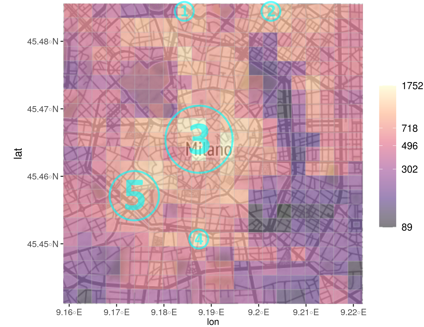
Figure 1: Average crowdedness measure over the period November 04, 2013, to November 11, 2013. The $x$-axis contains the longitude and the $y$-axis contains the latitude degrees. The marked areas represent:  Garibaldi Station,  Central Station,  Duomo,  Bocconi,  Navigli.

Figure 1 contains the crowdedness measure averaged over the 10-minute time intervals for the whole analyzed period over the $21\times 21$ grid. Areas with high levels of crowdedness are apparent in the central grid squares in the area surrounding the Milan Duomo and in the upper center, where the two main stations are, namely  Garibaldi Station and  Central Station. On the other hand, lower activity grid squares such as the ones overlaid on a highly trafficked avenue on the right-hand side and right bottom corner of the map can be identified.

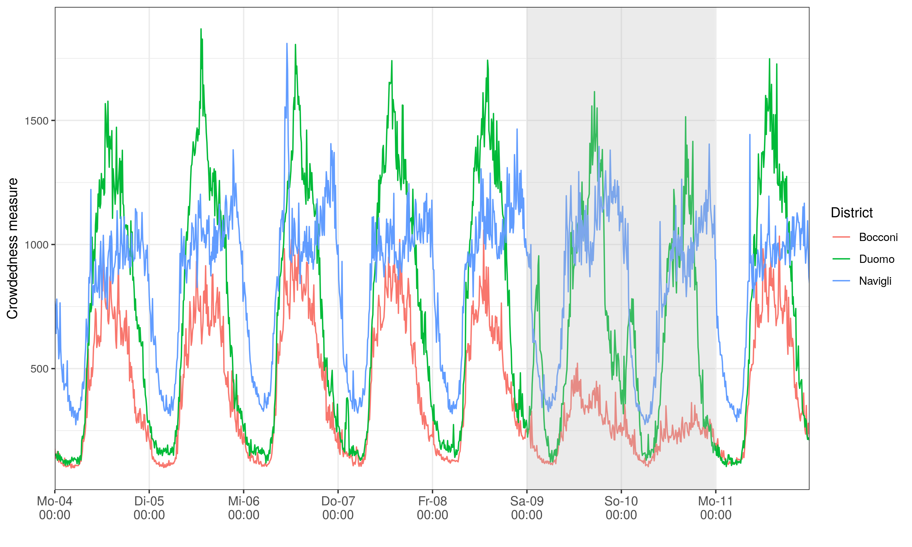
Figure 2: Time series of the crowdedness measure for the areal units containing the districts Duomo, Navigli and Bocconi over the period from November 04, 2013, to November 11, 2013. Areas marked in gray represent weekends.

In order to illustrate the temporal behavior of the crowdedness measure, we present in Figure 2 the time-series of the grid units containing the three representative districts of  Duomo,  Navigli and  Bocconi. We observe a larger high activity in the area of  Duomo compared to the other two districts, which peaks around midday during the working days and in the early afternoon on the weekends.  Navigli on the other hand, which is a district famous for its different types of cafés, restaurants, bars and design shops, exhibits a more uniform behavior among the working and the weekend days, with activity peaking in the evening hours. The grid square containing the  Bocconi university exhibits a clear pattern during the working hours and reduced activity levels on the weekends, especially on Sundays.

The seasonality in the data can be identified also in Figure 3, which contains a visualization of the whole dataset through a raster plot. Aside from the strong daily seasonality which is present in all locations, one can observe different temporal patterns among the areas. Most areas share the characteristic of a relatively lower activity in the weekends, while the activity in the working days differs among groups of locations e.g., the locations from the central part of the grid (cell IDs 150–280) exhibit a higher difference between the daily crowdedness during working days vs. weekends, while locations with cell IDs around 400 (top cells in the map) exhibit rather similar activity during the workdays and weekends.

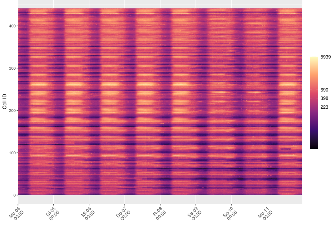
Figure 3: Raster plot exhibiting the time-series of the crowdedness measure for each of the 441 grid squares for the period November 04, 2013, to November 11, 2013.

5.2 Model comparison

In the following, we investigate and compare the predictive performance of the models introduced in Section 3. For this purpose, we set up an out-of-sample exercise based on rolling windows, where we start by training the Bayesian model on data between November 04, 2013, at 00:00 (Monday) and November 10, 2013 23:50 to generate one-, two- and three-step-ahead predictions, as well as for computing the predictive measures to be used for model selection for November 11, 2013 00:00 up to November 11, 2013 00:20. In a separate estimation procedure, we shift the window of the training data by 10 minutes and re-estimate the model in an iterative fashion until we reach the end of the sample.

In order to choose the dimension of the harmonic regressions, we inspect the estimated spectral densities of our $I=21\times 21=441$ time series (see Figure 4) and observe the strong intra-daily as well as an intra-weekly seasonality, with the largest values corresponding to 24 hour intervals. We use this information to select the 12 frequencies marked in by vertical lines in Figure 4 in constructing the harmonic regression. This means that the dimension of our vector of covariates $\bm{h}_{t}$ is 24.

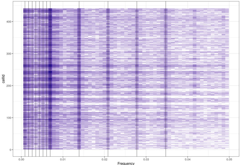
Figure 4: Raster plot exhibiting the spectral density estimates for each of the 441 grid squares for the period from November 04, 2013, to November 11, 2013. The $x$-axis only exhibits frequencies up to 0.05. The black vertical lines represent the frequencies which were chosen to be included in the harmonic regression after visual inspection of this graph. The chosen frequencies correspond to the intra-weekly and intra-daily seasonality.

As mentioned before, as a baseline model, we consider the model with no random effects $w_{i,t}=0$ and with one set of regression coefficients for all locations as the baseline. In addition to the CAR-AR-BNP model which performs clustering on the areal units, we consider three CAR-AR models which all assume a normal prior on $\bm{\beta}$: i) a model where the spatial auto-correlation parameter $\rho$ is fixed to $0$ – CAR-AR ($\rho=0$), ii) a model where spatial auto-correlation parameter $\rho$ is fixed to $0.5$ – CAR-AR ($\rho=0.5$), iii) a model where the spatial auto-correlation parameter $\rho$ is estimated in the MCMC procedure – CAR-AR.

For all models, the values of the hyperparameters are kept identical: $\bm{m}_{0}=\bm{0}$, $S_{0}=0.1\mathbb{I}_{2K}$, $a^{\sigma}=a^{\tau}=1$, $b^{\sigma}=b^{\tau}=0.01$. We take $\alpha=1$ in the BNP prior, and we use $C=50$ auxiliary variables in the algorithm for sampling the cluster assignments (see Section 3.2.1 in Favaro and Teh, 2013). All results are based on 10000 iterations of the Gibbs sampler, where the first 5000 are discarded as burn-in and the thinning parameter is set to 50. This leave 100 draws to be used for inference. The number of draws is not as large as typical values, but we use it to keep the verification of the properties (especially Property P.4) manageable in terms of computation time on a local computer. If one has access to a cluster of workstations, the number of iterations can be increased, as the property verification can trivially be parallelized. The trace plots of the models show acceptable convergence for all parameters, as well as good mixing.

Figure 5 presents the cumulative one-step ahead ($h=1$) and three-step ahead ($h=3$) log predictive Bayes factors for Monday, November 11, 2013:

$$\log\text{BF}_{t_{1},t_{2}}(A,B)=\sum_{t=t_{1}}^{t_{2}-h}\log\text{LPDS}_{t+h}(A)-\log\text{LPDS}_{t+h}(B),$$

where $B$ is taken to be a baseline model. We observe that all models which take space and/or time correlation into account through the autoregressive structure outperform the baseline model, with the model CAR-AR-BNP with spatial-clustering also outperforming, even if not by a lot, the CAR-AR model. In terms of the three-steps ahead prediction, the CAR-AR-BNP model is superior, but we observe also that the performance of all CAR-AR models is worse than the baseline in the hours following midnight and between 07:00-09:00 (see negative slopes in the log Bayes factor curves). Furthermore, the gain in performance of the CAR-AR models diminishes around 19:00, when the slopes of the curves are not as steep. These results point towards the fact that there might be a change in the spatial dependence parameter $\rho$ throughout the day. We leave such an extension of the model to further research.

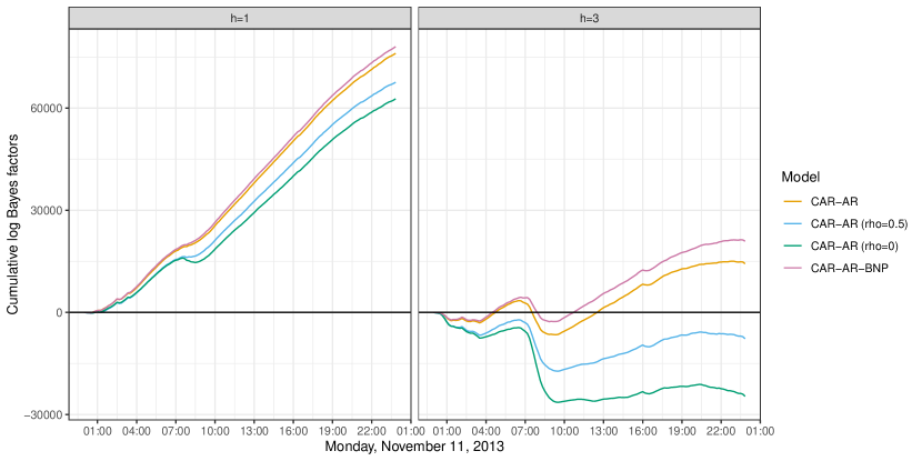
Figure 5: One- and three-steps-ahead cumulative log predictive Bayes factors for different models relative to the baseline model.

Finally, we also investigate the performance of the five models in terms of the predictive measures based on property satisfaction and robustness introduced in Section 2.3. The property parameters used for all properties are: $c=500$, $h_{\text{P.1}}=h_{\text{P.3}}=30~{}\text{min}$, $h_{\text{P.2}}=10~{}\text{min}$, $h_{\text{P.4}}=40~{}\text{min}$, $d_{\text{P.2}}=d_{\text{P.3}}=1~{}\text{cell}$, $d_{\text{P.4}}=4~{}\text{cells}$. Table 1 shows the posterior mean and standard deviation of the satisfaction accuracy, satisfaction F1 score and robustness RMSE for all four properties. We observe that the CAR-AR-BNP model is the best performing one in terms of the measures inspected, however the difference in performance for some properties is not large. Figure 6 presents the average value of the measures in Table 1 for all testing periods, together with 80% credible intervals. This figure can be used for deciding which model performs best in terms of specific interest in the verified properties. For example, it can be seen that the autoregressive models perform similarly in terms of satisfaction measures for all properties, while the robustness of the model CAR-AR-BNP is better for properties P.2 and P.3. The same model also outperforms the others in terms of property P.4 during the rush hours 07:00-09:00, so it should be chosen if the performance in this specific time-frame is of interest to the modeler.

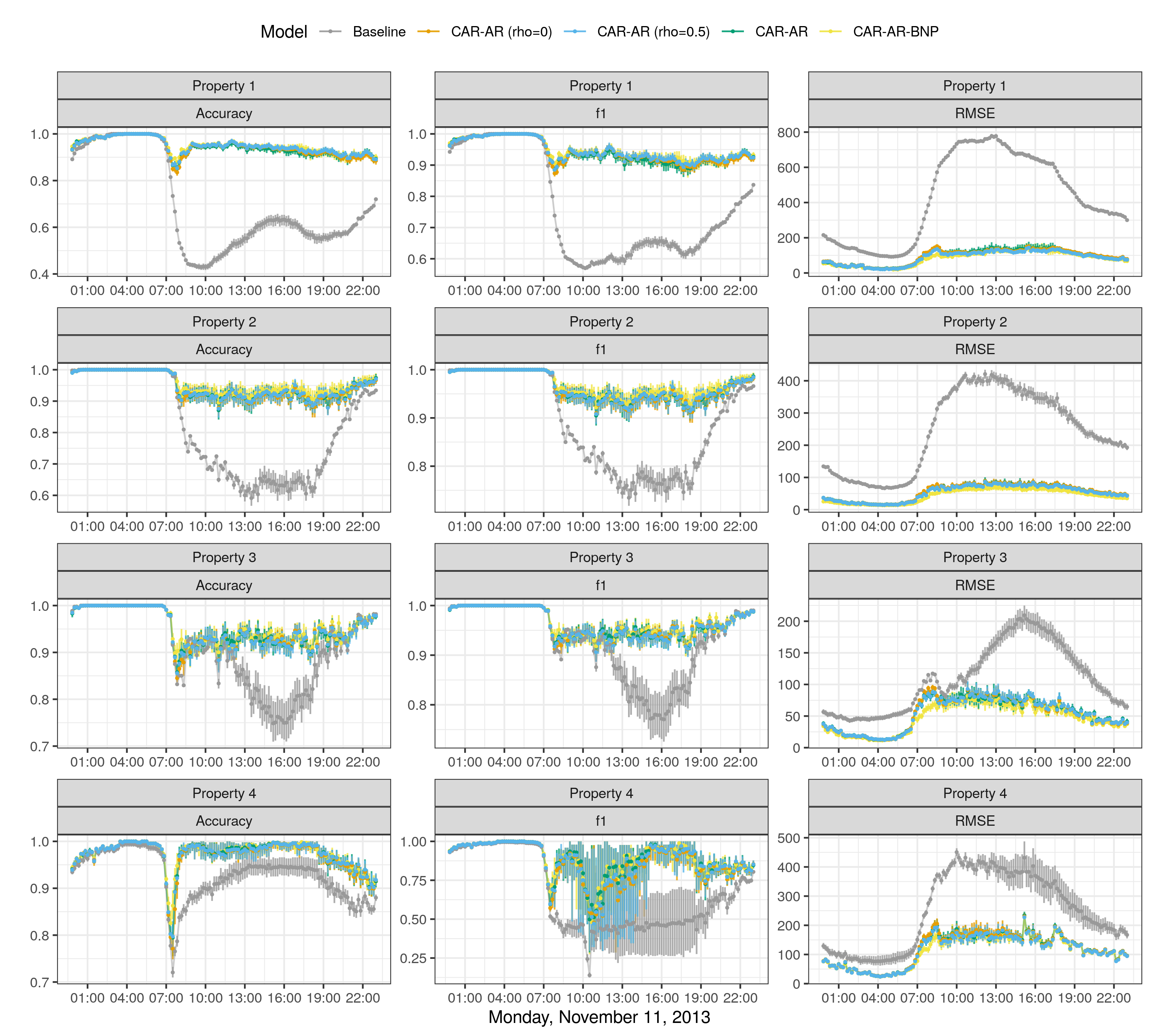
Figure 6: Mean accuracy, F1 score for the Bayesian predictive satisfaction measure and the RMSE of the robustness measure (points) with their corresponding 80% credible intervals for a rolling window exercise.

Table 1: Posterior means and standard deviations (in parentheses) of the predictive measures of accuracy and F1 scores for property satisfaction and the RMSE of the robustness for the four properties. The reported measures are averages over all test samples.

Measure	Baseline	CAR-AR	CAR-AR	CAR-AR	CAR-AR
		$\rho=0$	$\rho=0.5$		BNP
Property P.1
$\bar{\text{Acc}}^{\text{Satisf}}$	0.6999	0.944	0.9479	0.9445	0.9498
	(0.0056)	(0.0025)	(0.003)	(0.0059)	(0.0035)
$\bar{\text{F1}}^{\text{Satisf}}$	0.8027	0.9555	0.9584	0.956	0.9601
	(0.0029)	(0.0019)	(0.0022)	(0.0043)	(0.0026)
$\text{RMSE}^{\text{Rob}}$	493.2178	101.979	96.0108	101.7701	92.9006
	(5.84)	(3.8052)	(4.2172)	(9.328)	(6.104)
Property P.2
$\bar{\text{Acc}}^{\text{Satisf}}$	0.8177	0.9463	0.9481	0.9476	0.9553
	(0.0056)	(0.0038)	(0.0038)	(0.0043)	(0.0037)
$\bar{\text{F1}}^{\text{Satisf}}$	0.8988	0.9678	0.9688	0.9686	0.9731
	(0.0033)	(0.0022)	(0.0023)	(0.0025)	(0.0022)
$\text{RMSE}^{\text{Rob}}$	273.7798	59.9263	57.5646	59.1099	48.6895
	(8.4465)	(2.771)	(2.5964)	(2.7259)	(2.8436)
Property P.3
$\bar{\text{Acc}}^{\text{Satisf}}$	0.9116	0.9511	0.9508	0.9515	0.9547
	(0.0076)	(0.0028)	(0.0031)	(0.0036)	(0.0039)
$\bar{\text{F1}}^{\text{Satisf}}$	0.9439	0.9692	0.969	0.9695	0.9713
	(0.0051)	(0.0018)	(0.0021)	(0.0024)	(0.0026)
$\text{RMSE}^{\text{Rob}}$	120.5187	59.3011	59.1511	58.645	52.6133
	(7.339)	(1.9052)	(2.8903)	(3.8598)	(3.461)
Property P.4
$\bar{\text{Acc}}^{\text{Satisf}}$	0.9268	0.9703	0.9722	0.9726	0.9743
	(0.0061)	(0.0034)	(0.0037)	(0.0043)	(0.0034)
$\bar{\text{F1}}^{\text{Satisf}}$	0.8575	0.939	0.9426	0.9437	0.947
	(0.0117)	(0.007)	(0.0075)	(0.0084)	(0.0068)
$\text{RMSE}^{\text{Rob}}$	280.6554	130.225	125.8994	128.1106	122.4351
	(20.4942)	(6.0651)	(5.6114)	(6.5048)	(5.1467)

5.3 Results of the spatio-temporal model with spatial clustering

The top panel in Figure 7 presents the three clusters identified by employing Binder’s loss on the samples of the cluster assignments vector, while the bottom panel presents crowdedness measure averaged over all locations in one cluster. The blue cluster is one where the difference in the crowdedness between weekends and working days is not as large as for the other two, with activity peaking in the morning (stronger during the working days) as well as in the evening (stronger effect on Sunday). The  Navigli area is a member of the blue cluster. The yellow cluster contains areas where the activity is high in the working days and lower on the weekends, with an intraday peak around noon. Typical locations in this cluster are university centers or the city center, where most office buildings are situated. The green cluster is the smallest one, with the characteristic that the activity plummets during the weekend. The area corresponding to this cluster is Porta Romana, which contains the train station with the same name, a station primarily used by commuters into the city. Moreover, the rather isolated areas belonging to one cluster but enclosed by areas in other clusters seem to be explainable and likely not cause by model artifacts. For example, the yellow square in the middle of the green cluster is the location of a large shopping mall.

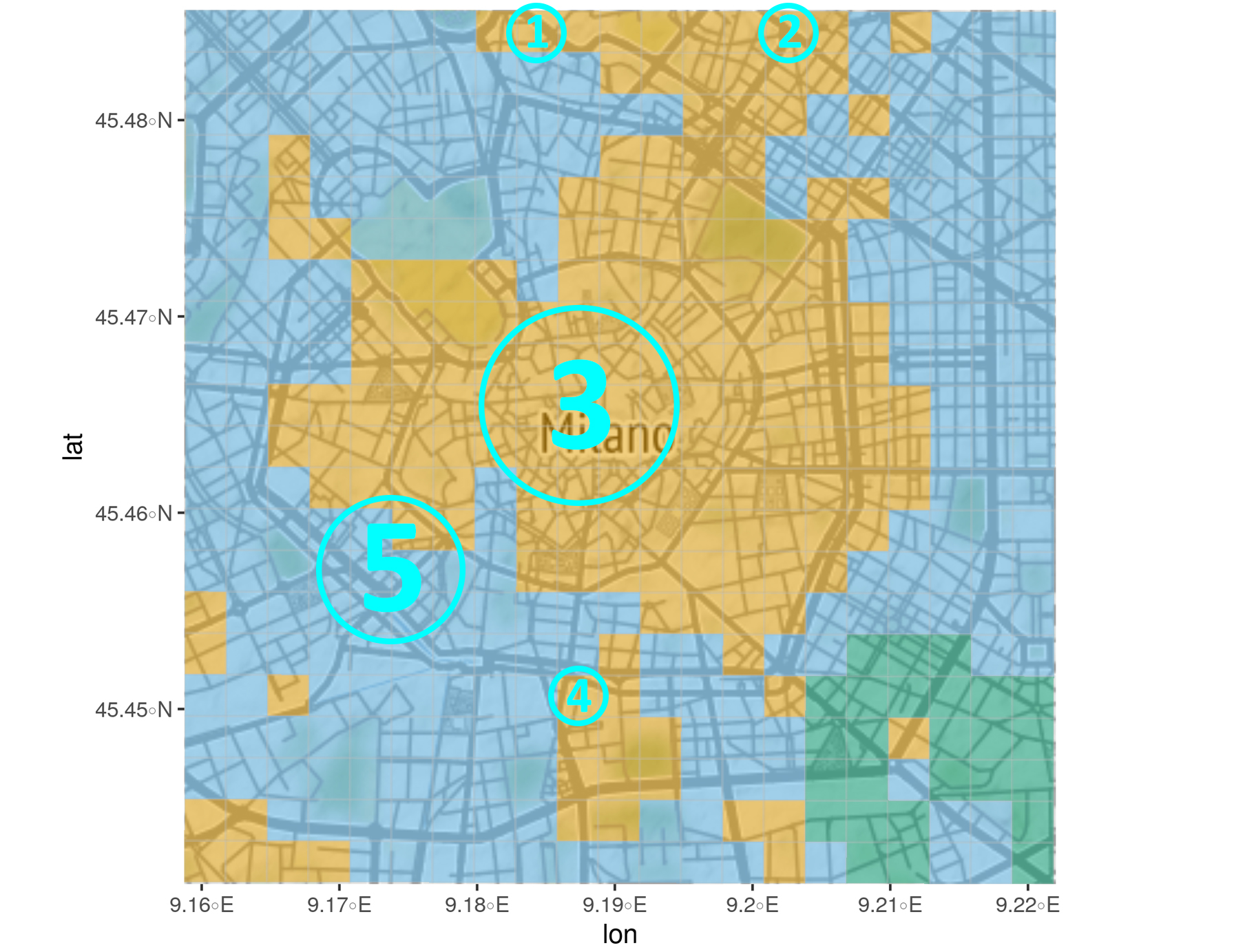
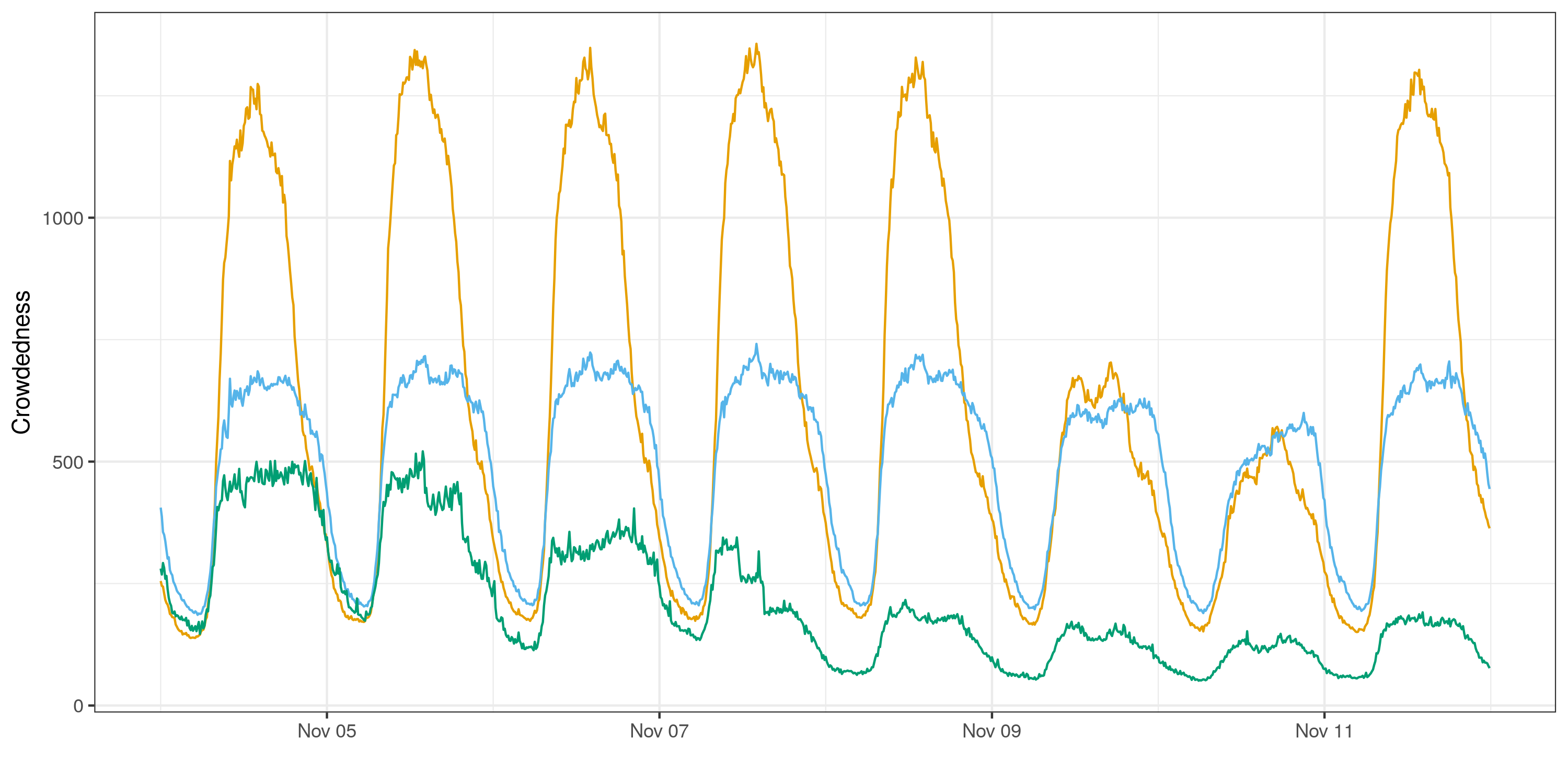
Figure 7: Top panel: Clusters as identified by Binder’s loss. Bottom panel: crowdedness measure averaged over all locations in one cluster

Finally, the spatial dependence parameter $\rho$ has a posterior mean of $0.9$ and the posterior mean of the $\xi$ parameter lies close to one, which indicates strong persistence in both space and time.

5.4 Verification of the crowdedness requirements for spatio-temporal model with spatial clustering

5.4.1 P.1 – Overloads are temporary

Figure 8 shows the estimated posterior satisfaction probability and the posterior mean of the robustness measure resulting from the evaluation of property P.1. Note that P.1 defines a property only in terms of a temporal operator, where we set $h_{\text{P.1}}=30~{}\text{min}$. That is, we check whether the crowdedness variable stays below a value of $c=500$ or, in case it exceeds this value, then it must return below it within 30 minutes. When looking at the results, it appears clear that the city is roughly split in two macro-areas: the historical and financial center is unlikely to satisfy the property during busy times, while the residential areas are almost always satisfying it. A relevant exception comes from the  Navigli area (left bottom of the map): it is, in fact, a vibrant area, where many young people live, which has many touristic landmarks and an active commercial area. We can see that this area is consistently violating our requirement over time, although, from a look at the robustness its actual value is close to zero, meaning that the violation is quite small, making it less concerning from a network capacity perspective.

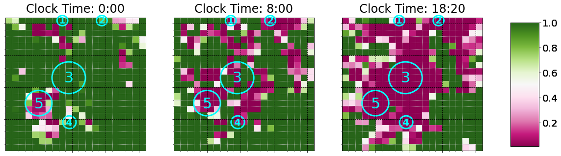
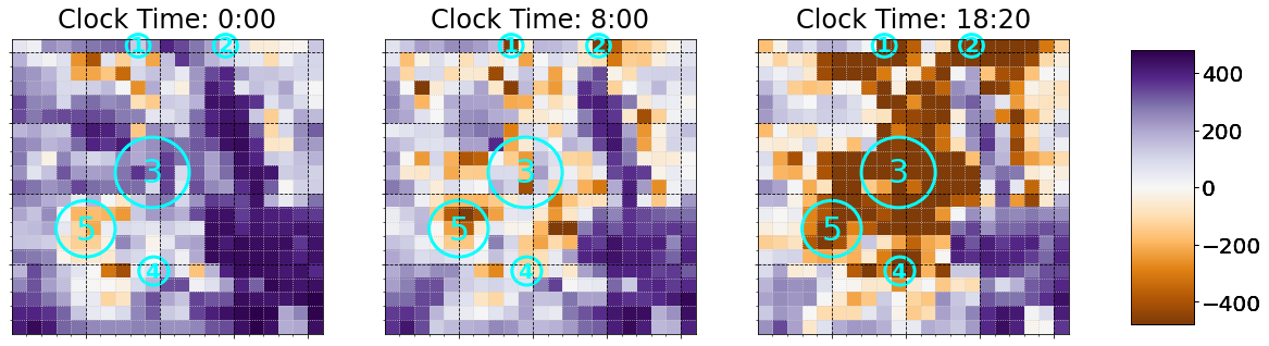
Figure 8: Posterior satisfaction probability (top row) and posterior mean of the robustness measure (bottom row) resulting from checking for property P.1 at three times of the day.

5.4.2 P.2 – Overloads are local

Figure 9 shows the estimated posterior satisfaction probability and the posterior mean of the robustness measure resulting from the evaluation of property P.2 at three different times of the day. Note that this property is based only on predictions of neighboring locations ($d_{\text{P.2}}=1~{}\text{cell}$) at future time $t+h_{\text{P.2}}$, with $h_{\text{P.2}}=10~{}\text{min}$. As one might intuitively expect, the property exhibits high values of satisfaction and robustness for a large area of the city center (there is usually at least an uncrowded area connected to a crowded one). A notable exception is the  Duomo area, from which crowds spread towards the other hot-spots at the busiest time of the day (18:20). However, by looking at the posterior predictive mean of the robustness for different time points, we get a more clear understanding about the spatial distribution of the excessive loads. In fact, it is evident that the  Duomo is the area that might most likely suffer from excessive crowdedness, without any possibility to enact load-balancing strategies based on the state of nearby locations. Conversely, other areas, like the  Navigli area, have a much safer spatial behavior, either because they exceed the threshold only slightly, or because they are surrounded by areas with much lower levels of crowdedness.

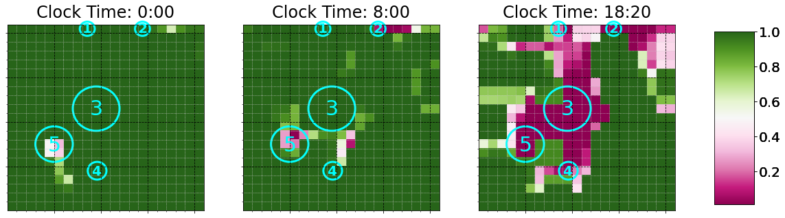
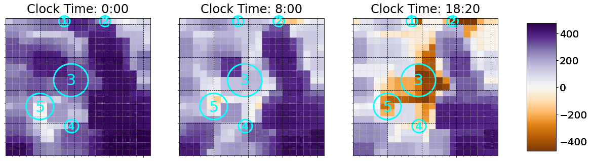
Figure 9: Posterior satisfaction probability (top row) and posterior mean of the robustness measure (bottom row) resulting from checking property P.2 at three times of the day.

5.4.3 P.3 – The network is fault-tolerant

Figure 10 shows the estimated posterior satisfaction probability and the posterior mean of the robustness measure resulting from the evaluation of property P.3 at three different times of the day. Property P.3 enforces the availability of a neighboring uncrowded area (i.e., $d_{\text{P.}3}=1$) consistently for $h_{\text{P.}3}=30~{}\text{min}$. The first thing the reader might notice is that this property exhibits a visual pattern similar to P.1–P.2, except that it is in general less likely to be satisfied. This behavior is to be expected, as one can notice when looking at the logic formulas: P.3 resembles, in fact, the structure of the right side of implication (“$\rightarrow$”) in P.1–P.2, except that it enforces stricter requirements (there must be an uncrowded area for the next half-hour). This observation shows a key strength of logic for the validation and explainability of specifications: from an informal perspective, P.1 and P.2 describe different aspects than P.3. Yet, the obtained results show that P.3 could effectively replace P.1–P.2 as a specification that encompasses both of them. In fact, P.3 summarizes the ideal behavior of a fault-tolerant system overall. Verifying this property clearly shows that the city is split into two parts, with the most-touristic part less likely to satisfy the property, while the residential and non-touristic areas are more likely to satisfy it.

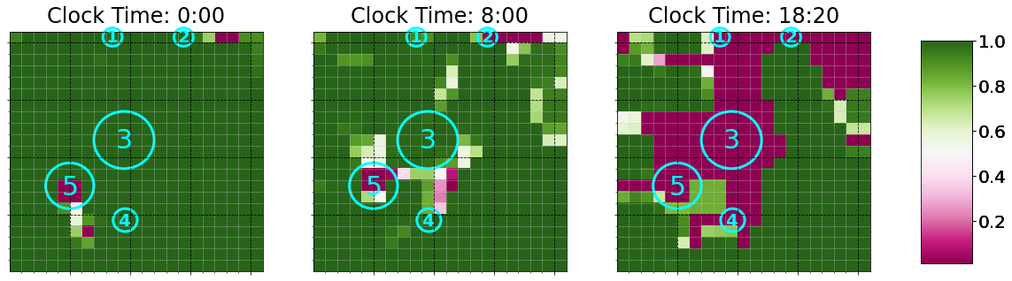
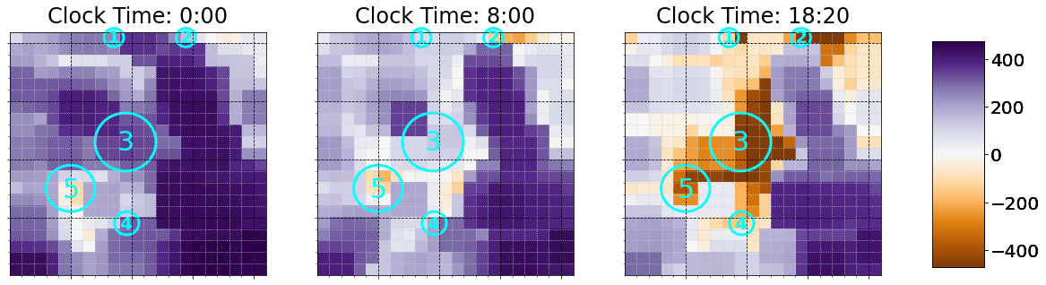
Figure 10: Posterior satisfaction probability (top row) and posterior mean of the robustness measure (bottom row) resulting from checking property P.3 at three times of the day.

5.4.4 P.4 – Uncrowded reachability

Figure 11 presents the results of verifying property P.4 for $h_{\text{P.4}}=40\text{min}$ and $d_{\text{P.4}}=4~{}\text{cells}$ (approximately $1$ km).

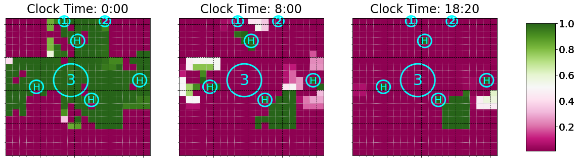
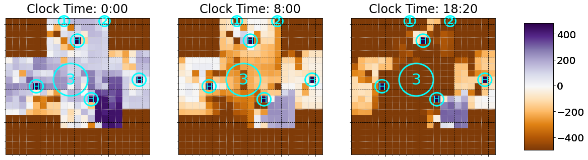
Figure 11: Posterior satisfaction probability (top row) and posterior mean of the robustness measure (bottom row) resulting from monitoring the property P.4 at three times of the day.

circles mark hospitals’ locations, where the property is trivially satisfied in all circumstances. By looking at the picture, an immediate observation is that areas at the corners are simply too far from any of the city center hospitals, meaning that going towards the center from there would be impractical. However, it is interesting to see that, while it is never very easy to get to hospitals in busy times (like at 18:20), the  Central Station is still in a good spot (as it is not too far, and not too crowded), conversely the  Garibaldi Station is in a less favorable location, as it becomes practically inaccessible in crowded times. Even worse is the  Duomo area, which, despite being quite close to a hospital, experiences such high levels of crowdedness that make reaching the hospital almost impossible in crowded times (in the terms of the requirement we have defined), while it is relatively easier in medium-crowded times. Lastly, the always failing areas at the corners of the grid, and at the bottom-center tell us something different: for the spatial configuration we are considering, they always violate the requirement to reach a hospital of the city center in $d_{\text{P.}4}$. This can be surprising at first, but a look at the broader map of the city clarifies that they are closer to hospitals that are not in our grid, therefore cannot be fully analyzed by our model.

6 Discussion and future work

In this paper we propose a framework for predictive model checking and comparison, where in addition to usual approaches, we advocate for the specification of concrete (spatio-temporal) properties which the predictions from a model should satisfy. Given trajectories from the Bayesian predictive distribution, the posterior predictive probability of satisfaction and the posterior predictive robustness of these properties can be approximated by verifying the properties on each of the trajectories efficiently using techniques from formal verification methods. Finally, we can evaluate ex post the model by comparing the resulting measures with the values in the observed data.

We illustrate the approach by building a Bayesian spatio-temporal model for areal crowdedness extracted from aggregated mobile phone data in the city of Milan and by formulating properties which the crowdedness level in the city network should satisfy in order to robustly withstand critical events. We compare various model specifications which include a harmonic regression with and without random effects, as well as a model which performs clustering of the area-specific harmonic regression coefficients. The model which performs clustering is indeed the one which performs best in terms of the proposed measures. This model can however be further refined to clustering over time or a temporal evolution of the persistence parameter for the autoregressive random effects.

The proposed framework advocates for exploiting the rich information that Bayesian predictive inference offers in the form of draws from the posterior predictive distribution of future values, by evaluating models also based on properties which can be directly translated into decision-making. Therefore, we show-case how different model specifications are then evaluated based on well-known performance measures but also on posterior predictive measures employed in formal verification, such as the satisfaction probabilities or the robustness measure.

On a larger scale, by exploiting the synergy between Bayesian modeling and formal verification methods, we also advocate for the development and use of explainable algorithms where properties relevant for decision-making are incorporated into the data analytic process flow. Therefore, the proposed approach has a clear potential in the area of sustainable cities and urban mobility, as these applications deal with complex systems, with a multitude of stakeholders and with a pressing need for transparency in the decision-making process. We hope for the illustration in the current paper to open the way to further applications.

Computational details and replication materials

The computations have been performed on 25 IBM dx360M3 nodes within a cluster of workstations. Instruction for downloading the data set as well as an extensive description can be found in Barlacchi et al. (2015). The estimation of the Bayesian models can be performed using code in the repository https://github.com/lauravana/CARBayesSTBNP. The Moonlight tool is available at https://github.com/moonlightsuite/moonlight, while the specific problem instance related to this project, together with the data and the scripts for generating the figures, are available at: https://github.com/ennioVisco/bayesformal.

[Acknowledgments] The authors acknowledge funding from the Austrian Science Fund (FWF) for the project “High-dimensional statistical learning: New methods to advance economic and sustainability policies” (ZK 35), jointly carried out by the University of Klagenfurt, the University of Salzburg, TU Wien, and the Austrian Institute of Economic Research (WIFO).

References

- Banerjee (2017) Banerjee, S. (2017). “High-dimensional Bayesian geostatistics.” Bayesian Analysis, 12(2): 583 – 614.
- Barlacchi et al. (2015) Barlacchi, G., De Nadai, M., Larcher, R., Casella, A., Chitic, C., Torrisi, G., Antonelli, F., Vespignani, A., Pentland, A., and Lepri, B. (2015). “A multi-source dataset of urban life in the city of Milan and the Province of Trentino.” Scientific data, 2(1): 1–15.
- Bernardo and Smith (1994) Bernardo, J. M. and Smith, A. F. (1994). Bayesian Theory. John Wiley & Sons.
- Bernini et al. (2019) Bernini, A., Toure, A. L., and Casagrandi, R. (2019). “The time varying network of urban space uses in Milan.” Applied Network Science, 4(1): 1–16.
- Bonato et al. (2020) Bonato, P., Cintia, P., Fabbri, F., Fadda, D., Giannotti, F., Lopalco, P. L., Mazzilli, S., Nanni, M., Pappalardo, L., Pedreschi, D., et al. (2020). “Mobile phone data analytics against the COVID-19 epidemics in Italy: flow diversity and local job markets during the national lockdown.” arXiv preprint arXiv:2004.11278.
- Bürkner et al. (2020) Bürkner, P.-C., Gabry, J., and Vehtari, A. (2020). “Approximate leave-future-out cross-validation for Bayesian time series models.” Journal of Statistical Computation and Simulation, 90(14): 2499–2523.
- Cadonna et al. (2019) Cadonna, A., Cremaschi, A., and Guglielmi, A. (2019). “Bayesian modeling for large spatio-temporal data: an application to mobile networks.” In Smart Statistics for Smart Applications. Book of Short Papers SIS 2019, 691–696. Pearson.
- Cinnamon et al. (2016) Cinnamon, J., Jones, S. K., and Adger, W. N. (2016). “Evidence and future potential of mobile phone data for disease disaster management.” Geoforum, 75: 253–264.
- Clarke and Emerson (1982) Clarke, E. M. and Emerson, E. A. (1982). “Design and synthesis of synchronization skeletons using branching time temporal logic.” In Kozen, D. (ed.), Logics of Programs, 52–71. Berlin, Heidelberg: Springer Berlin Heidelberg.
- Corradi and Swanson (2006) Corradi, V. and Swanson, N. R. (2006). “Predictive density evaluation.” In Elliott, G., Granger, C., and Timmermann, A. (eds.), Handbook of Economic Forecasting, volume 1 of Handbook of Economic Forecasting, 197–284. Elsevier.
- Deville et al. (2014) Deville, P., Linard, C., Martin, S., Gilbert, M., Stevens, F. R., Gaughan, A. E., Blondel, V. D., and Tatem, A. J. (2014). “Dynamic population mapping using mobile phone data.” Proceedings of the National Academy of Sciences, 111(45): 15888–15893.
- Fainekos and Pappas (2009) Fainekos, G. E. and Pappas, G. J. (2009). “Robustness of temporal logic specifications for continuous-time signals.” Theoretical Computer Science, 410(42): 4262–4291.
- Favaro and Teh (2013) Favaro, S. and Teh, Y. W. (2013). “MCMC for normalized random measure mixture models.” Statistical Science, 28(3): 335–359.
- Frazier et al. (2021) Frazier, D. T., Loaiza-Maya, R., Martin, G. M., and Koo, B. (2021). “Loss-based variational Bayes prediction.” arXiv preprint arXiv:2104.14054.
- Gariazzo et al. (2019) Gariazzo, C., Pelliccioni, A., and Bogliolo, M. P. (2019). “Spatiotemporal analysis of urban mobility using aggregate mobile phone derived presence and demographic data: a case study in the city of Rome, Italy.” Data, 4(1).
- Gelman et al. (1996) Gelman, A., Meng, X.-L., and Stern, H. (1996). “Posterior predictive assessment of model fitness via realized discrepancies.” Statistica Sinica, 733–760.
- Geweke and Amisano (2010) Geweke, J. and Amisano, G. (2010). “Comparing and evaluating Bayesian predictive distributions of asset returns.” International Journal of Forecasting, 26(2): 216–230.
- Gneiting and Raftery (2007) Gneiting, T. and Raftery, A. E. (2007). “Strictly proper scoring rules, prediction, and estimation.” Journal of the American Statistical Association, 102(477): 359–378.
- Iqbal et al. (2014) Iqbal, M. S., Choudhury, C. F., Wang, P., and González, M. C. (2014). “Development of origin–destination matrices using mobile phone call data.” Transportation Research Part C: Emerging Technologies, 40: 63–74.
- Kastner (2016) Kastner, G. (2016). “Dealing with stochastic volatility in time series using the R package stochvol.” Journal of Statistical Software, 69(5): 1–30.
- Knorr-Held and Rue (2002) Knorr-Held, L. and Rue, H. (2002). “On block updating in Markov random field models for disease mapping.” Scandinavian Journal of Statistics, 29(4): 597–614.
- Krüger et al. (2021) Krüger, F., Lerch, S., Thorarinsdottir, T., and Gneiting, T. (2021). “Predictive inference based on Markov chain Monte Carlo output.” International Statistical Review, 89(2): 274–301.
- Legay et al. (2019) Legay, A., Lukina, A., Traonouez, L. M., Yang, J., Smolka, S. A., and Grosu, R. (2019). Statistical Model Checking, 478–504. Cham: Springer International Publishing.
- Leroux et al. (2000) Leroux, B. G., Lei, X., and Breslow, N. (2000). “Estimation of disease rates in small areas: a new mixed model for spatial dependence.” In Statistical models in epidemiology, the environment, and clinical trials, 179–191. Springer.
- Matheson and Winkler (1976) Matheson, J. E. and Winkler, R. L. (1976). “Scoring rules for continuous probability distributions.” Management Science, 22(10): 1087–1096.
- McCausland et al. (2011) McCausland, W. J., Miller, S., and Pelletier, D. (2011). “Simulation smoothing for state-space models: A computational efficiency analysis.” Computational Statistics & Data Analysis, 55(1): 199–212.
- Mozdzen et al. (2022) Mozdzen, A., Cremaschi, A., Cadonna, A., Guglielmi, A., and Kastner, G. (2022). “Bayesian modeling and clustering for spatio-temporal areal data: an application to Italian unemployment.” arXiv preprint arXiv:2206.10509.
- Nenzi et al. (2022) Nenzi, L., Bartocci, E., Bortolussi, L., and Loreti, M. (2022). “A logic for monitoring dynamic networks of spatially-distributed cyber-physical systems.” Logical Methods in Computer Science, 18(1).
- Nenzi et al. (2020) Nenzi, L., Bartocci, E., Bortolussi, L., Loreti, M., and Visconti, E. (2020). “Monitoring spatio-temporal properties.” In Deshmukh, J. and Ničković, D. (eds.), Runtime Verification, 21–46. Cham: Springer International Publishing.
- Nenzi et al. (2017) Nenzi, L., Bortolussi, L., Ciancia, V., Loreti, M., and Massink, M. (2017). “Qualitative and quantitative monitoring of spatio-temporal properties with SSTL.” arXiv preprint arXiv:1706.09334.
- Peters-Anders et al. (2017) Peters-Anders, J., Khan, Z., Loibl, W., Augustin, H., and Breinbauer, A. (2017). “Dynamic, interactive and visual analysis of population distribution and mobility dynamics in an urban environment using the mobility explorer framework.” Information, 8(2): 56.
- Queille and Sifakis (1982) Queille, J. P. and Sifakis, J. (1982). “Specification and verification of concurrent systems in CESAR.” In Dezani-Ciancaglini, M. and Montanari, U. (eds.), International Symposium on Programming, 337–351. Berlin, Heidelberg: Springer Berlin Heidelberg.
- Rubin (1984) Rubin, D. B. (1984). “Bayesianly justifiable and relevant frequency calculations for the applied statistician.” The Annals of Statistics, 1151–1172.
- Savitsky and Williams (2022) Savitsky, T. D. and Williams, M. R. (2022). “Bayesian dependent functional mixture estimation for area and time-indexed data: an application for the prediction of monthly county employment.” Bayesian Analysis, 17(3): 791 – 815.
- Vehtari et al. (2017) Vehtari, A., Gelman, A., and Gabry, J. (2017). “Practical Bayesian model evaluation using leave-one-out cross-validation and WAIC.” Statistics and Computing, 27(2): 1413––1432.
- Wang et al. (2021) Wang, Z., Yue, Y., He, B., Nie, K., Tu, W., Du, Q., and Li, Q. (2021). “A Bayesian spatio-temporal model to analyzing the stability of patterns of population distribution in an urban space using mobile phone data.” International Journal of Geographical Information Science, 35(1): 116–134.
- Wardrop et al. (2018) Wardrop, N., Jochem, W., Bird, T., Chamberlain, H., Clarke, D., Kerr, D., Bengtsson, L., Juran, S., Seaman, V., and Tatem, A. (2018). “Spatially disaggregated population estimates in the absence of national population and housing census data.” Proceedings of the National Academy of Sciences, 115(14): 3529–3537.
- Younes et al. (2006) Younes, H. L. S., Kwiatkowska, M., Norman, G., and Parker, D. (2006). “Numerical vs. statistical probabilistic model checking.” International Journal on Software Tools for Technology Transfer, 8(3): 216–228.
- Zuliani et al. (2013) Zuliani, P., Platzer, A., and Clarke, E. M. (2013). “Bayesian statistical model checking with application to Stateflow/Simulink verification.” Formal Methods in System Design, 43(2): 338–367.