CENN: Conservative energy method based on neural networks with subdomains for solving variational problems involving heterogeneous and complex geometries

Abstract

We propose a conservative energy method based on neural networks with subdomains for solving variational problems (CENN), where the admissible function satisfying the essential boundary condition without boundary penalty is constructed by the radial basis function (RBF), particular solution neural network, and general neural network. Loss term is the potential energy, optimized based on the principle of minimum potential energy. The loss term at the interfaces has the lower order derivative compared to the strong form PINN with subdomains. The advantage of the proposed method is higher efficiency, more accurate, and less hyperparameters than the strong form PINN with subdomains. Another advantage of the proposed method is that it can apply to complex geometries based on the special construction of the admissible function. To analyze its performance, the proposed method CENN is used to model representative PDEs, the examples include strong discontinuity, singularity, complex boundary, non-linear, and heterogeneous problems. Furthermore, it outperforms other methods when dealing with heterogeneous problems.

1 Introduction

Many physical phenomena are modeled by partial differential equations (PDEs). In general, it is difficult to obtain the analytical solutions of PDEs. Hence, various numerical methods are developed to obtain the approximate solutions in a finite dimensional space. Traditional ways to tackle the solution of PDEs are the finite element method (FEM), the finite difference method, the finite volume method, and mesh-free method [1]. The traditional methods, especially FEM, are computationally efficient and accurate for engineering applications. However, mesh generation of complex boundaries [2], dimensional explosion and distortion problems for the high-dimensional cases cannot be tackled well by FEM [3], reducing the efficiency exponentially lower. In addition, FEM requires the selection of specific basis functions to construct the approximation function. For example, the singular element specifically is designed for fracture mechanics singularities [4] in FEM. Constructing basis functions corresponding to different elements undoubtedly increases the brainpower cost.

Artificial intelligence has impacted many fields in the last decade, and it is now generally expected that the means to achieve artificial intelligence can be machine learning, using data-driven optimization. Deep learning, a method in machine learning, has achieved unprecedented success in many fields, from computer vision [5], speech recognition [6], natural language processing [7], and strategy games [8, 9] to drug development[10] . In the present day, deep learling is ubiquitous, empowering various fields. The success of deep learning partially attributes to the powerful approximation capabilities of the neural network [11]. It is natural to use the neural network as the approximation function of PDEs, i.e., physics-informed neural network (PINN) [12].

The idea of using the neural network to solve PDEs can be traced back to the last century [13], but it received little attention due to hardware limitations. Raissi et al. propose PINN to deal with the strong form of the PDE, i.e., a weighted residual method with neural networks as the approximate function [12]. PINN can apply to many physical systems containing PDEs. In [14], a framework using PINN was proposed for the solution of forward and inverse problems in solid mechanics. In [15], PINN is used to approximate the Euler equations that model high-speed aerodynamic flows in fluid mechanics. In [16], the theory of error bound estimation in the incompressible Navier-Stokes equations is proposed for PINN. In [17], PINN is used to infer properties of biological materials. In [18], PINN is used to solve the composite material physical system of thermochemical. A library named “DeepXDE” using PINN was developed to facilitate the use of scientific machine learning [19]. The loss function in PINN is contructed with the PDEs in the domain, boundary conditions, and initial conditions by weighted sum of the squared errors. Different choices of trial function and test function correspond to various numerical methods, eg. trial function with domain decomposition [20] and test function with domain decomposition [21]. The advantage of PINN strong form is less dependent on sampling size in every iteration, only requiring zero loss at any given coordinate point [22]. Since all PDEs have a weighted residual form, the strong form is general and can solve almost all PDEs. Another framework of PINN is the deep energy form [22, 23, 24, 25, 26, 1, 27], using the physical potential energy as the optimized loss function. The advantage of deep energy method (DEM) is that the physical interpretation is stronger than PINN strong form. In addition, DEM requires less hyperparameters than strong form. By virtue of a smaller derivative order than the strong form, the computational efficiency and accuracy are higher. The disadvantage of DEM is dependent on the choice of the integration scheme for the energy integration, in order to make the numerical integration of energy as accurate as possible [22, 23]. DEM lacks in generality, not all PDEs have a corresponding energy form [4].

Most of the current research is focused on the strong form of PINN, the research about the energy form is relatively limited. There are too many hyperparameters in the strong form of PINN, especially CPINN (space subdomains) [20] and XPINN (space-time subdomains for arbitrary complex-geometry domains) [28], so we often need to adjust hyperparameters empirically [22, 23]. Although there are currently valuable research results [29, 30, 31] for the selection of hyperparameters, the optimal hyperparameters still cannot be attained accurately when faced with specific problems. The main advantage of domain decomposition of PINN is the flexibility of optimizing all hyperparameters of each neural network separately in each subdomain, so the parallel algorithms can be used to increase the training speed [32]. On the other hand, the possible displacement field in the DEM is often constructed by a penalty factor $\beta$, i.e., $\beta\cdot MSE(u^{pred},\bar{u})$ [26], or multiplying coordinates, i.e., $x\cdot u^{pred}$ (u=0, when x=0) to satisfy the special geometry essential boundary such as the beam [1, 25]. In [2, 23, 33], the possible displacement field is constructed by distance network and particular solution network in PINN. Sukumar et al. researched the exact imposition of boundary conditions based on the distance function for the both PINN strong form and energy form [34]. Some of the earlier studies on PINN to construct the admissible function can be traced to the contributions of Lagaris et al. [35]. Although PINN strong form with subdomains (CPINN) already exists, it lacks PINN energy form with subdomains.

In this work, we propose a conservative energy form based on neural networks with subdomains for solving variational problems (CENN), where the admissible function is constructed by the radial basis function (RBF), particular solution neural network, and general neural network. This method of constructing the admissible function is suitable for the complexity boundary problem. To the best of my knowledge, this is the first attempt to leverage the power of PINN energy form to the heterogeneous problem, including discontinuity, singularity, high-order tensor, high-order derivative, and nonlinear PDEs problem. The advantages of the CENN are multi-fold :

• Efficient handling of heterogeneous problems: Unlike traditional DEM, CENN can handle the strong discontinuity and derivative discontinuity problem on the interface by assigning the different neural networks in each subdomain. It is worth noting that the interface loss in CPINN, has more terms than CENN , which will be mentioned in detail in Section 3.

• Hyperparameter fewer: According to the variational principle, CENN writes the PDEs in the domain as an energy functional and does not consider the hyperparameters of the different PDEs in domains as CPINN to piece PDEs together. In addition, CENN considers fewer interface conditions at the interface than CPINN, which are derived in detail in section 3.2. Therefore, the hyperparameters of CENN are fewer than CPINN. The advantage of fewer hyperparameters is that CENN can reduce the cost of adjusting hyperparameters.

• Complex geometries: In CENN, the admissible function satisfying the essential boundary condition without boundary penalty is constructed by the RBF, particular solution neural network, and general neural network. CENN can apply to complex geometries based on the special construction of the admissible function.

• Accuracy and efficiency: Due to the lower derivative in CENN, the accuracy and efficiency are higher than the strong form. In addition, the independent part between the subdomains can be implemented by a parallelization algorithm, which will further improve efficiency.

• Less brainpower cost: CENN benefits from the expressive power of the neural network. So we need not construct the approximation function by designing a basis function, e.g. the special elements in FEM.

• The ability to solve distortion problems: CENN is a mesh-free method, so it has the same advantage as the mesh-free method. The proposed algorithm is quite effective in distortion.

• Flexibility of the subdomains configuration: CENN can divide the region to different neural networks. The different configurations, such as the number of hidden layers, activation function, can be assigned to the different neural networks for the specific problems.

The outline of the paper is as follows. Section 2 is a revision of the prerequisite knowledge. It provides a brief introduction to feed-forward neural network, PINN, and the DEM. Section 3 describes the methodology of the proposed method CENN. The strategy is explained for constructing the admissible function based on the RBF and particular network. In Section 4, some of the representative applications of CENN are presented:

1. The crack problem shows that the proposed method can solve the strong discontinuity and singularity problem well, where data-driven and CPINN are compared with CENN.

2. The complex boundary and heterogeneous problem verifies the proposed method has the feasibility of complex boundary and derivative discontinuity problems, where various comparisons are made between CPINN, DEM and, CENN.

3. The non-linear hyperelasticity problem with composite materials proves the proposed method can deal with non-linear PDEs, where various comparisons are made between FEM, DEM, and CENN.

Section 5 shows the discussion. Finally, Section 6 concludes the study by summarizing the key results of the present work.

2 Prerequisite knowledge

In this section, we provide an overview of the feed-forward neural network. Next, we introduce the main idea of the PINN. In the end, we give an outline of the deep energy method (DEM).

2.1 Inroduction to feed-forward neural network

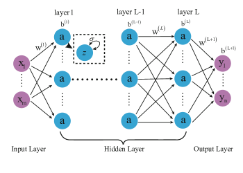
(a)

Figure 1: Schematic of fully neural network, the left purple circles in the neural network are the inputs. Blue circles in the neural network are the hidden neurons. The right purple circles in the neural network are the output neurons. $\boldsymbol{x}$ and $\boldsymbol{y}$ are the input and output representively. $\boldsymbol{z}$ is the linear output. $\boldsymbol{\sigma}$ is the activation function acting on $\boldsymbol{z}$. $\boldsymbol{w}$ and $\boldsymbol{b}$ are the parameters of the neural network.

The feed-forward neural network is a multiple linear regression with the activation function aimed to increase the non-linear ability. Fig. 1 shows a schematic diagram of feed-forward neural network. The feed-forward neural network is given by

$$\begin{split}\boldsymbol{z}^{(1)}&=\boldsymbol{w}^{(1)}\cdot\boldsymbol{x}+\boldsymbol{b}^{(1)}\\ \boldsymbol{a}^{(1)}&=\boldsymbol{\sigma}(\boldsymbol{z}^{(1)})\\ \vdots\\ \boldsymbol{z}^{(L)}&=\boldsymbol{w}^{(L)}\cdot\boldsymbol{a}^{(L-1)}+\boldsymbol{b}^{(L)}\\ \boldsymbol{a}^{(L)}&=\boldsymbol{\sigma}(\boldsymbol{z}^{(L)})\\ \boldsymbol{y}&=\boldsymbol{w}^{(L+1)}\cdot\boldsymbol{a}^{(L)}+\boldsymbol{b}^{(L+1)}\end{split}$$ (1)

where $\boldsymbol{z^{(l)}}$ is the linear transformation of the previous neurons $\boldsymbol{a^{(l-1)}}$, the layers $1\leq l\leq L$ are the hidden layers. $\boldsymbol{a^{(l)}}$is the output of $\boldsymbol{z^{(l)}}$ through the activation function $\sigma$, and the activation function $\sigma$ is a non-linear function, such as tanh, sigmoid. In this article, we uniquely use the tanh function as the activation function

$$tanh=\frac{e^{x}-e^{-x}}{e^{x}+e^{-x}}.$$ (2)

where $\boldsymbol{w^{(m)}}$ is the weight between the layer m-1 and m. $\boldsymbol{b^{(m)}}$ is the bias of the layer m.

2.2 Introduction to Physics-Informed Neural Network

(a)

Figure 2: Schematic of PINN, the left purple circles in the neural network are the inputs (temporal and spatial coordinates). The right blue circles in the neural network are the hidden neurons. The right purple circles in the neural network are the output (interesting field). $\boldsymbol{L(\cdot)}$ is the differential operator related to the PDEs. $\bar{\boldsymbol{u}}$ is the given data including boundary and initial condition. MSE is the mean square error to let the interesting field to satisfy the essential boundary. $\lambda_{r}$ and $\lambda_{b}$ are the weight of the residual loss $Loss_{r}$ and the boundary loss $Loss_{b}$ (including initial condition if temporal problem) respectively. PINN updates the parameters of neural network until the loss is less than the threshold.

In this section, we give the outline for physics-informed neural network (PINN). The schematic of the PINN is shown in Fig. 2. PINN uses neural networks as the approximation function. PDEs related to the specific problem are the guide of the loss function construction. The boundary and initial conditions are required in advance. The $Loss_{b}$ is the discrepancy between exact solution and neural network approximation, which commonly uses MSE as the criterion to satisfy the essential boundary. Then the $Loss_{r}$ is the difference between the known PDEs and the neural network approximation, where the differential operators are regularly constructed by the Automatic Differentiation [36] to get the differential terms in PDEs, which provides exact derivatives while bypassing the computational expense and accuracy issues of symbolic and numercial differentiation [37]. Fortunately, the packages such as Tensorflow and Pytorch [38] have the function inherently and conveniently, so it is convenient to construct the $Loss_{b}$ related to the PDEs. The whole loss function reads as :

$$\mathcal{L}=\frac{\lambda_{r}}{N_{r}}\sum_{i=1}^{N_{r}}|\boldsymbol{L}\boldsymbol{u}(\boldsymbol{x}_{i};\boldsymbol{\theta})|{}^{2}+\frac{\lambda_{b}}{N_{b}}\sum_{i=1}^{N_{b}}||\boldsymbol{u}(\boldsymbol{x}_{i};\theta)-\bar{\boldsymbol{u}}(\boldsymbol{x}_{i})||_{2}^{2}$$ (3)

where $\boldsymbol{u}(\boldsymbol{x};\boldsymbol{\theta})$ is the prediction of the coordinate point $\boldsymbol{x}$ with the neural network parameters $\boldsymbol{\theta}$. $\boldsymbol{x}$ is the coordinate (spatial and temporal) which is being used as the input of the neural network; $\boldsymbol{\theta}$ is the neural network parameter obtained by the optimization of the loss function. $\boldsymbol{L}$ is the differential operator, which can be the linear or non-linear differential operator. $\boldsymbol{Lu}(\boldsymbol{x};\boldsymbol{\theta})$ is the PDE equation using the neural network as the interesting field $\boldsymbol{u}$. $\bar{\boldsymbol{u}}(\boldsymbol{x})$is the boundary or initial condition data known in advance. $N_{r}$ and $N_{b}$ are the number of the residual points and the boundary data points respectively. $\lambda_{r}$ and $\lambda_{b}$ represent the corresponding weight of the residual loss $Loss_{r}$ and the boundary loss $Loss_{b}$ respectively

$$\begin{split}\mathcal{L}_{r}&=\frac{1}{N_{r}}\sum_{i=1}^{N_{r}}|\boldsymbol{L}\boldsymbol{u}(\boldsymbol{x}_{i};\boldsymbol{\theta})|{}^{2}\\ \mathcal{L}_{b}&=\frac{1}{N_{b}}\sum_{i=1}^{N_{b}}||\boldsymbol{u}(\boldsymbol{x}_{i};\boldsymbol{\theta})-\bar{\boldsymbol{u}}(\boldsymbol{x}_{i})||_{2}^{2}\end{split}$$ (4)

2.3 Introduction to deep energy method

We introduce the variational principle firstly. Then we explain how to combine the PINN with the principle of minimum potential energy.

If PDEs has variational formulation, the solution of the strong form is equal to the variational formulation, i.e., the solution $\boldsymbol{u}$ of strong form makes $J(\boldsymbol{u})$ stationary with respect to the arbitrary changes $\delta\boldsymbol{u}$ [4], where $J(\boldsymbol{u})$ represent the functional and $\boldsymbol{u}$ is a trial function satisfying the essential boundary condition. If neural network loss is the functional, we can get the solution of the strong form by optimization the loss

$$\mathcal{L}=J(\boldsymbol{u})$$ (5)

$$\boldsymbol{u}^{DEM}(\boldsymbol{x};\boldsymbol{\theta})=min_{\boldsymbol{\theta}}J(\boldsymbol{u}(\boldsymbol{x};\boldsymbol{\theta}))\approx min_{\boldsymbol{u}}J(\boldsymbol{u}),$$ (6)

where $\boldsymbol{u}^{DEM}$ is the solution of the DEM. Although the function space of the neural network is enormous, there might still be the approximation error, i.e., the error between the true function space and the PINN function space depending on the neural network configuration. $\boldsymbol{\theta}$ is the parameter of the neural network. It is worth noting that $\boldsymbol{u}$ must satisfy the essential boundary condition, i.e., Dirichlet boundary condition.

Remark 1.

the trial function $\boldsymbol{u}$ must satisfy the essential boundary condition,

$$\boldsymbol{u}(\boldsymbol{x})=\bar{\boldsymbol{u}}(\boldsymbol{x}),\boldsymbol{x}\subseteq\varGamma^{\boldsymbol{u}},$$ (7)

where $\varGamma^{\boldsymbol{u}}$ is the essential boundary, and $\bar{\boldsymbol{u}}(\boldsymbol{x})$ is the given essential boundary value. In addition, $\boldsymbol{u}(\boldsymbol{x})\in H^{m}$ if the differential operator has order $2m$, where $H$ is the Sobolev space.

3 Method

3.1 construction of the admissible function

The penalty method can be used to satisfy the essential boundary condition softly, but the additional hyperparameter called the penalty factor has to be considered. The most critical challenge of the penalty method is that the best penalty is not precisely known in advance. Therefore, it is necessary to construct the admissible function

$$\boldsymbol{u}(\boldsymbol{x})=\boldsymbol{u}_{p}(\boldsymbol{x};\boldsymbol{\theta}_{p})+RBF(\boldsymbol{x})\cdot\boldsymbol{u}_{g}(\boldsymbol{x};\boldsymbol{\theta}_{g})$$ (8)

where $\boldsymbol{u}_{p}(\boldsymbol{x};\boldsymbol{\theta}_{p})$ called particular network is a common shallow network trained on the essential boundary to minimize the following MSE loss

$$\mathcal{L}_{p}=\frac{1}{n_{be}}\sum_{i=1}^{n_{be}}(\boldsymbol{u}_{p}(\boldsymbol{x}_{i};\boldsymbol{\theta}_{p})-\bar{\boldsymbol{u}}(\boldsymbol{x}_{i}))^{2}$$ (9)

$n_{be}$ is the number of the essential boundary points.

$RBF(\boldsymbol{x})$ called distance network is a radial basis function to give the nearest distance from $\boldsymbol{x}\in\Omega$ to $\varGamma^{\boldsymbol{u}}$, where $\Omega$ denotes the domain of interest field.

Many of the methods approximate the distance function by neural networks [33, 2], which is a universal scheme to approximate the distance function for any complex-shaped boundaries. However, such a treatment of the essential boundary condition is not straightforward since an extra training process is required for neural networks. Considering that the distance function of the analytical solution is not complex in simple structures, it indeed does not need neural networks with a large amount of iterative calculation to approximate the distance function. The neural networks is suitable for complex boundaries and RBF is suitable for simple boundaries.

The number of RBF distribution points and the arrangement need to be determined according to the geometric shape of the essential boundary. Here, we adopt the commonly used Gaussian function as the basis function :

$$RBF(\boldsymbol{x})=\sum_{i=1}^{n}w_{i}\phi(|\boldsymbol{x}-\boldsymbol{x}_{i}|),$$ (10)

where $w_{i}$ is the weight of the center $\boldsymbol{x}_{i}$ in RBF. The value of $w_{i}$ can be obtained according to the training set {$\boldsymbol{x}_{i}$, $y_{i}$} , $y_{i}$ is the label of $\boldsymbol{x}_{i}$, which is the nearest distance to the essential boundary. $\boldsymbol{x}$ is the coordinate to be evaluated. The following linear equations determine $w_{i}$,

$$\left[\begin{array}[]{cccc}\phi(|\boldsymbol{x}_{1}-\boldsymbol{x}_{1}|)&\phi(|\boldsymbol{x}_{1}-\boldsymbol{x}_{2}|)&\cdots&\phi(|\boldsymbol{x}_{1}-\boldsymbol{x}_{n}|)\\ \phi(|\boldsymbol{x}_{2}-\boldsymbol{x}_{1}|)&\phi(|\boldsymbol{x}_{2}-\boldsymbol{x}_{2}|)&&\vdots\\ \vdots&&\ddots&\phi(|\boldsymbol{x}_{n-1}-\boldsymbol{x}_{n}|)\\ \phi(|\boldsymbol{x}_{n}-\boldsymbol{x}_{1}|)&\cdots&\phi(|\boldsymbol{x}_{n}-\boldsymbol{x}_{n-1}|)&\phi(|\boldsymbol{x}_{n}-\boldsymbol{x}_{n}|)\end{array}\right]\text{$\left[\begin{array}[]{c}w_{1}\\ w_{2}\\ \vdots\\ w_{n}\end{array}\right]$=$\left[\begin{array}[]{c}y_{1}\\ y_{2}\\ \vdots\\ y_{n}\end{array}\right]$},$$ (11)

where $\phi(|\boldsymbol{x}-\boldsymbol{x}_{i}|)$ is named after the radial basis function. Since this function is completely determined by the distance between $\boldsymbol{x}$ and $\boldsymbol{x}_{i}$ regardless of the direction from $\boldsymbol{x}$ to $\boldsymbol{x}_{i}$, that is the reason called radial. Since the displacement function needs to be derived, there is a higher requirement for the continuity of the distance function. However, the analytical distance function is C0 continuous (at the medial axis of the domina, the displacement function is shape) [34], so the analytical displacement function is not suitable to use in PINN theoretically. Therefore, we choose Gaussian kernel function as the basis function, which ensures the continuity of higher order. Note that the displacement function does not need to be exactly the same as the analytical solution, but only if it is equal to zero on the essential boundary, which guarantees that the inhomogeneous boundary condition is satisfied. Gaussian kernel is:

$$\phi(r)=exp(-\gamma r^{2})$$ (12)

In this article, we adopt $\gamma=0.5$ as the shape parameter empirically, because the optimal shape parameter is often located at the small scope. At present, the basis function and shape parameter in RBF mainly depend on experience, and there is no good theoretical guidance [39, 40]. It is appropriate that the placement of the RBF points reflect the given value surface as well as possible. A good placement of the center points improves the accuracy of the approximation function. We use a uniform distribution way due to the simplicity (other collocation ways: Halton and epsilon collocation) [40]. The method of box counting can be adopted to determine the number of collocation points. Box counting is a kind of a method to determine the complexity of space [41]. For example, we can use the box counting to determine the complexity of the essential boundary conditions. The number of collocation points can be proportional to the box counting, because the large box counting means a more complex the boundary (the more points are needed). The number of center points $\{\boldsymbol{x}_{i},y_{i}\}$ commonly often does not need to take much to construct the distance network, as shown in the later numerical experiment. It is not difficult to prove that the radial basis matrix on the LHS of Equation 11 is invertible if the coordinates of the center points are different. RBF method can accurately satisfy the label value $y_{i}$ of the fixed point $\boldsymbol{x}_{i}$. The label value $y_{i}$ can be obtained in advance using kdtree [2] or other methods. The accuracy can be improved by increasing the RBF center points, but it will increase the amount of calculation.

$\boldsymbol{u}_{g}(\boldsymbol{x};\boldsymbol{\theta}_{g})$ in Equation 8 called general network is the regulator to let the functional $J(\boldsymbol{u})$ minimum. $\boldsymbol{u}_{g}(\boldsymbol{x};\boldsymbol{\theta}_{g})$ is also a neural network, whose architecture and activation can be determined according to the specific problem. Note that the form of Equation 8 ensures that $\boldsymbol{u}(\boldsymbol{x})$ satisfies the essential boundary condition if the particular and distance network have been trained successfully. We can see the later numerical experiments show it is easy to train the particular and the distance network successfully. It is important that the admissible function can solve the complex boundary problem, which will be discussed in detail in Section 4.2. PINN energy method must meet the admissible function before using the principle of minimum potential energy to optimize the potential energy (loss function), as shown in Fig. 3.

Remark 2.

The parameter of the particular and the distance network, which should be trained before the general network in advance, must be fixed (untrainable ) when training the general network. The order of particular and distance network does not matter.

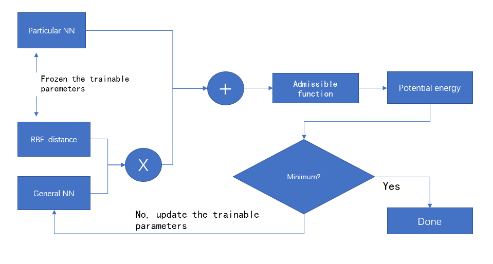
(a)

Figure 3: The overall process of PINN energy form.

3.2 CENN

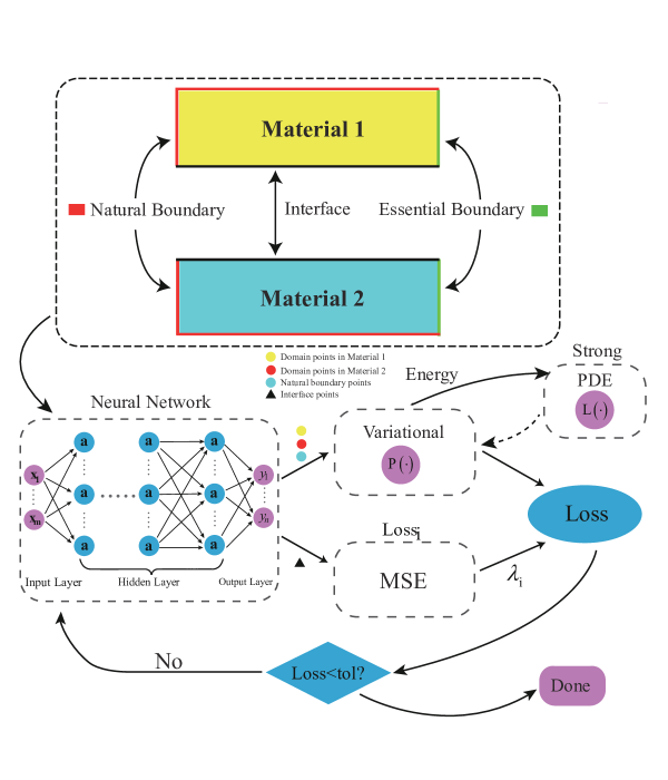
(a)

Figure 4: Schematic of CENN : The green lines in the upper picture are the essential boundary points, which is used to train the admissible function. The red lines in the upper picture are the natural boundary points. The yellow and blue region in the upper picture are the domain points corresponding to the different material. The interface points are the black line in the upper picture. $\boldsymbol{L}(\cdot)$ is the differential operator related to the PDE strong form. $\boldsymbol{P}(\cdot)$ is the differential operator related to the energy form, whose order of derivative is lower than the strong form. $\lambda_{i}$ is the weight of the interface term. The input is the coordinates. The output is the field of interest. The loss function is the energy functional. The energy functionals of different materials are connected through the interface loss.

In this section, we introduce our proposed method CENN (conservative energy neural network for solving variational problems), and the difference with CPINN (Conservative physics-informed neural networks). Notes, CENN is only used for the PDEs that have variational formulation, but CPINN can be used for almost any PDEs. Note that CENN is based on the principle of the minimum potential energy, so it only can solve the static problem.

Fig. 4 shows the schematic of CENN. CENN is a deep energy method with subdomains and an admissible function. The way to construct the admissible function is illustrated in Section 3.1. The solution is obtained by optimizing the energy function. The energy function adds the additional term called interface loss, which ensures the conservative physic law.

We consider the heterogeneous PDEs governing equation :

$$\begin{split}\boldsymbol{L}(\boldsymbol{u};a_{i})+\boldsymbol{f}_{i}=0,&\boldsymbol{x}\subseteq\Omega_{i}\\ \boldsymbol{u}(\boldsymbol{x})=\boldsymbol{\bar{u}}(\boldsymbol{x}),&\boldsymbol{x}\subseteq\varGamma^{\boldsymbol{u}}\\ \boldsymbol{B}(\boldsymbol{u};a_{i})=\boldsymbol{\bar{t}},&\boldsymbol{x}\subseteq\varGamma^{\boldsymbol{t}_{i}}\\ \boldsymbol{B}(\boldsymbol{u};a^{+})=\boldsymbol{B}(\boldsymbol{u};a^{-}),&\boldsymbol{x}\subseteq\varGamma^{inter}\\ \boldsymbol{u}^{+}(x)=\boldsymbol{u}^{-}(x),&\boldsymbol{x}\subseteq\varGamma^{inter},\end{split}$$ (13)

where $\boldsymbol{L}$ is the differential operator. $\boldsymbol{u}$ is an interesting tensor field. $a_{i}$ is the coefficient of $\boldsymbol{L}(\boldsymbol{u};a_{i})$ in the different region $\Omega_{i}$. $\boldsymbol{u}(\boldsymbol{x})=\boldsymbol{\bar{u}}(\boldsymbol{x})$ is the essential boundary condition, and $\boldsymbol{\bar{u}}$ is the given value of the essential boundary condition (Dirichlet boundary condition). $\boldsymbol{B}(\boldsymbol{u};a_{i})=\bar{\boldsymbol{t}}$ is the natural boundary condition, and $\bar{\boldsymbol{t}}$ is the given value of the natural boundary condition (Neumann boundary condition). $\Omega$, $\varGamma^{\boldsymbol{u}}$, $\varGamma^{\boldsymbol{t}}$ and $\varGamma^{inter}$ are the domain, essential boundary, natural boundary and interface respectively. The subscript $i$ represent the different region. The $+$ and $-$ represent the regions on either side of the interface. We can get the corresponding integral Galerkin form,

$$\begin{split}\int_{\Omega_{i}}(\boldsymbol{L}(\boldsymbol{u};a_{i})+\boldsymbol{f}_{i})\cdot\delta\boldsymbol{u}d\Omega+\int_{\varGamma^{t_{i}}}(\boldsymbol{B}(\boldsymbol{u};a_{i})-\bar{t})\cdot\delta\boldsymbol{u}d\varGamma\\ \int_{\varGamma^{inter}}(\boldsymbol{B}(\boldsymbol{u};a^{+})-\boldsymbol{B}(\boldsymbol{u};a^{-}))\cdot\delta\boldsymbol{u}d\varGamma+\int_{\varGamma^{inter}}(\boldsymbol{u}^{+}-\boldsymbol{u}^{-})\cdot\delta\boldsymbol{u}d\varGamma&=0,\end{split}$$ (14)

If the operator $\boldsymbol{L}$ satisfies

$$\int_{\Omega}\boldsymbol{L}(\boldsymbol{u})\cdot\boldsymbol{v}d\Omega =\int_{\Omega}\boldsymbol{u}\cdot\boldsymbol{L}^{*}(\boldsymbol{v})d\Omega+b.t.(\boldsymbol{u},\boldsymbol{v})$$ (15)

$$\boldsymbol{L}(a\boldsymbol{u_{1}}+b\boldsymbol{u_{2}}) =aL(\boldsymbol{u_{1}})+bL(\boldsymbol{u_{2}}),$$ (16)

we call the differential operator is self-adjointness and linear operator [4]. We assume $\boldsymbol{L}$ is the self-adjointness and linear operator. We use integration by parts and obtain

$$\delta J=0$$ (17)

where

$$J=\int_{\Omega_{i}}[\frac{1}{2}\boldsymbol{u}\cdot\boldsymbol{L}(\boldsymbol{u};a_{i})+\boldsymbol{u}\cdot\boldsymbol{f}]d\Omega+\int_{\varGamma^{inter}}(\boldsymbol{u}^{+}-\boldsymbol{u}^{-})^{2}d\varGamma+b.t.(\boldsymbol{u})$$ (18)

Remark 3.

If the differential operator is linear and self-adjoint, and the highest differential operator order is even, then strong form must have the corresponding minimum potential energy formualtion, i.e., the energy formulation is extreme value problem [4]. In other words, all strong form have a weak form, but only the linear, self-adjoint and even order differiential operator problem have the corresponding minumum potential energy formulation.

For the sake of simplicity, we consider the specific PDEs,

$$\begin{split}-a_{i}\triangle(u(\boldsymbol{x}))=0,&\boldsymbol{x}\subseteq\Omega_{i}\\ u(\boldsymbol{x})=\bar{u}(\boldsymbol{x}),&x\subseteq\varGamma^{u}\\ \boldsymbol{n}\cdot a_{i}(\nabla u(\boldsymbol{x}))=\bar{t}(\boldsymbol{x}),&\boldsymbol{x}\subseteq\varGamma^{t_{i}}\\ \boldsymbol{n}\cdot(a^{+}(\nabla u(\boldsymbol{x}))=\boldsymbol{n}\cdot(a^{-}(\nabla u(\boldsymbol{x})),&\boldsymbol{x}\subseteq\varGamma^{inter}\\ u^{+}(\boldsymbol{x})=u^{-}(\boldsymbol{x}),&\boldsymbol{x}\subseteq\varGamma^{inter}\end{split}$$ (19)

where $\triangle$ is the Laplace operator. The interesting field $u$ is a scalar or tensor, for the sake of simplicity, we consider $u$ as a scalar. $\bar{u}$ is the given value of the essential boundary condition (Dirichlet boundary condition). $\bar{t}$ is the natural boundary condition (Neumann boundary condition). $\Omega$, $\varGamma^{u}$, $\varGamma^{t}$ and $\varGamma^{inter}$ is the domain, essential bound, natural boundary and interface respectively. $a$ is the coefficients of PDE and constant in the different regions. The subscript $i$ represent the different region. $n$ is the normal direction of the Neumann boundary and the interface. For the sake of simplicity, we analyze two different regions denoted as $+$ and $-$. The variation form is constructed by an integral Galerkin form

$$\begin{split}\int_{\Omega^{+}}-a^{+}(\triangle u)\delta ud\Omega+\int_{\Omega^{-}}-a^{-}(\triangle u)\delta ud\Omega\\ +\int_{\varGamma^{t+}}(\boldsymbol{n}\cdot a^{+}(\nabla u)-\bar{t})\delta ud\varGamma+\int_{\varGamma^{t-}}(\boldsymbol{n}\cdot a^{-}(\nabla u)-\bar{t})\delta ud\varGamma\\ +\int_{\varGamma^{inter}}\boldsymbol{n}\cdot(a^{+}(\nabla u)-a^{-}(\nabla u))\delta ud\varGamma+\int_{\varGamma^{inter}}(u^{+}-u^{-})\delta ud\varGamma&=0\end{split}$$ (20)

where $\boldsymbol{u}$ statisfies the essential boundary in advance. We integrate the Equation 20 by parts, and we can get the weak form with the interface term

$$\begin{split}\int_{\Omega^{+}}a^{+}(\nabla u)\cdot(\nabla\delta u)d\Omega+\int_{\Omega^{-}}a^{-}(\nabla u)\cdot(\nabla\delta u)d\Omega\\ -\int_{\varGamma^{t+}+\Pi^{+}}a^{+}\boldsymbol{n}\cdot(\nabla u)\delta ud\varGamma-\int_{\varGamma^{t-}+\Pi^{-}}a^{-}\boldsymbol{n}\cdot(\nabla u)\delta ud\varGamma\\ +\int_{\varGamma^{t+}}(\boldsymbol{n}\cdot a^{+}(\nabla u)-\bar{t})\delta ud\varGamma+\int_{\varGamma^{t-}}(\boldsymbol{n}\cdot a^{-}(\nabla u)-\bar{t})\delta ud\varGamma\\ +\int_{\varGamma^{inter}}\boldsymbol{n}\cdot(a^{+}(\nabla u)-a^{-}(\nabla u))\delta ud\varGamma+\int_{\varGamma^{inter}}(u^{+}-u^{-})\delta ud\varGamma&=0\end{split}$$ (21)

where $\Omega^{+}$ and $\Omega^{-}$ are the different regions of the interesting field. $\varGamma^{+}$ and $\varGamma^{-}$ are Newmann boundaries of the different region without the interface. $\Pi^{+}$ and $\Pi^{-}$are the interface $\varGamma^{inter}$ of the different region, overlapping each other, and $\boldsymbol{n}$ is the normal direction of the region $\Omega^{+}$ on the interface, i.e., $\boldsymbol{n}=\boldsymbol{n}^{+}=-\boldsymbol{n}^{-}$. We combine the similar items

$$\begin{split}\int_{\Omega^{+}}a^{+}(\nabla u)\cdot(\nabla\delta u)d\Omega+\int_{\Omega^{-}}a^{-}(\nabla u)\cdot(\nabla\delta u)d\Omega\\ -\int_{\varGamma^{t+}}\bar{t}\delta udx-\int_{\varGamma^{t-}}\bar{t}\delta ud\varGamma+\int_{\varGamma^{inter}}(u^{+}-u^{-})\delta ud\varGamma&=0.\end{split}$$ (22)

The Equation 22 is equal to the energy stationary, so we can get the energy form with the interface,

$$\begin{split}J&=\frac{1}{2}\int_{\Omega^{+}}a^{+}(\nabla u)\cdot(\nabla u)d\Omega+\frac{1}{2}\int_{\Omega^{-}}a^{-}(\nabla u)\cdot(\nabla u)d\Omega\\ &-\int_{\varGamma^{t+}}\bar{t}ud\varGamma-\int_{\varGamma^{t-}}\bar{t}ud\varGamma+\beta\int_{\varGamma^{inter}}(u^{+}-u^{-})^{2}d\varGamma\end{split}$$ (23)

where $\beta$ is the hyperparameter of the interface. Further, the above energy form is a convex function, and the exact solution is the stationary point, i.e., the extreme value problem. Although the energy form is convex in terms of the whole function space, it is commonly not convex in the neural network function space. So we can get the solution by optimizing J to a minimum. We can assign the different neural network in each subdomain. The backpropagation of CENN is discussed in A. CENN penalty only has one unknown penalty on the interface to ensure the continuity of the interesting field. However, CPINN not only has the $\boldsymbol{u}$ continuity condition but also has the derivative of $\boldsymbol{u}$ continuity condition. The additional derivative of CPINN will decrease the accuracy and efficiency. If the order of the PDE increase, the additional term about interface will increase in CPINN more than CENN, e.g., if the order of PDE is $2m$ order derivative, it is easy to prove that CPINN will have m more interface penalty factors than CENN. Although there are currently some theoretical guidances for the selection of hyperparameters [29, 30, 31], there are still many challenges to determine the hyperparameters, i.e., the different components of the loss function. Compared with the CPINN, the penalty of CENN is greatly reduced, but there is still a penalty of the interface, which is a hyperparameter. Here we use a heuristic construction

$$\beta=-c\cdot ln(tanh(\frac{N_{interface}}{N_{domain}}))$$ (24)

where $c$ is a scale factor, we recommend 1e3. $N_{interface}$ and $N_{domain}$ are the number of points at the interface and the domain respectively. The Equation 24 uses the concept of information entropy, we assume that $p=tanh(N_{interface}/N_{domain})$ is the probability of the certainty of the interface. Obviously, the more interface points, the greater certainty of probability about the interface. The training is essentially multi-task learning, therefore it is a game between the interface loss and the energy functional. If there are more interface points, less attention has been paid to energy functional training. We need to adjust the hyperparameter $\beta$ to balance the interface loss and energy loss. Finally, $-ln(p)$ is the information entropy to evaluate the value of the interface information, i.e., it indicates that the interface has more abundant information if there are more interface points. The above heuristic construction is used to construct the penalty of the interface. After many numerical experiments, we found that training is successful by this construction of the hyperparameter.

Remark 4.

CENN is suitable for solving the problem of one point coordinate containing multiple values of interesting field, such as the crack problem, which will be mentioned in detail in Section 4.1. CENN is also suitable for solving the problem of weak continuity problem, i.e., the original function is continuous but the derivative function is discontinuous, such as heterogeneous problem, which will be mentioned in detail in Section 4.2 and Section 4.3.

Remark 5.

DEM is a special form of the weighted residual. The test functuion of DEM and traditional PINN is $\partial u(\boldsymbol{x};\boldsymbol{\theta})/\partial\theta_{j}$ and $2\triangle\partial u(\boldsymbol{x};\boldsymbol{\theta})/\partial\theta_{j}$ respectively.

For the sake of simplicity, we consider the Poisson equation with the whole essential boundary

$$\triangle u=f.$$ (25)

The energy form of the strong form is

$$\mathcal{L} =\sum_{i=1}^{n^{v}}w_{i}w_{\varepsilon}(u_{1}(\boldsymbol{x}_{i};\boldsymbol{\theta}))-\sum_{i=1}^{n^{v}}w_{i}f_{i}u(\boldsymbol{x}_{i};\boldsymbol{\theta})$$ (26)

where $w_{i}$ is the weight of the attribution points $\boldsymbol{x}_{i}$, especially $w_{i}=V/n$ if uniform random Monte Carlo method is adopted. $w_{\varepsilon}=\frac{1}{2}(\nabla u)\cdot(\nabla u)$, $u$ is a scalar interesting variable. The first-order variation w.r.t. Loss is

$$\delta\mathcal{L} =\sum_{i=1}^{n^{v}}\frac{V}{n}(\nabla u_{i})\cdot(\nabla\delta u_{i})-\sum_{i=1}^{n^{v}}\frac{V}{n}f_{i}\delta u_{i}$$ (27)

The first term on the RHS is integrated by parts. We can get

$$\begin{split}\delta\mathcal{L}&=\sum_{i=1}^{n^{v}}\frac{V}{n}(\triangle u_{i})(\delta u_{i})-\sum_{i=1}^{n^{v}}\frac{V}{n}f_{i}\delta u\\ &=\sum_{i=1}^{n^{v}}\frac{V}{n}(\triangle u_{i}-f_{i})(\delta u_{i}).\end{split}$$ (28)

Given the trial function $u$ is an admissible function, the boundary part generated by integrating by parts with $\delta u$ is vanish. Considering the interesting field $u$ is the function of neural network parameter $\theta$, the variation form can be rewritten

$$\begin{split}\delta\mathcal{L}&=\sum_{i=1}^{n^{v}}\frac{V}{n}(\triangle u_{i}-f_{i})(\sum_{j=1}^{n^{\theta}}\frac{\partial u_{i}}{\partial\theta_{j}}\delta\theta_{j})\\ &=\sum_{j=1}^{n^{\theta}}\sum_{i=1}^{n^{v}}\frac{V}{n}(\triangle u_{i}-f_{i})(\frac{\partial u_{i}}{\partial\theta_{j}}\delta\theta_{j}).\end{split}$$ (29)

The stationary point (the first-order variation is zero) is equal to the strong form with the test function $\partial u(x;\theta)/\partial\theta_{j}$, j=1, 2, . . . $n^{\theta}$, i. e. ,

$$\begin{split}\mathcal{L}_{1}&=\sum_{i=1}^{n^{v}}\frac{V}{n}(\triangle u_{i}-f_{i})(\frac{\partial u_{i}}{\partial\theta_{1}})\\ \mathcal{L}_{2}&=\sum_{i=1}^{n^{v}}\frac{V}{n}(\triangle u_{i}-f_{i})(\frac{\partial u_{i}}{\partial\theta_{2}})\\ \vdots\\ \mathcal{L}_{n^{\theta}}&=\sum_{i=1}^{n^{v}}\frac{V}{n}(\triangle u_{i}-f_{i})(\frac{\partial u_{i}}{\partial\theta_{n^{\theta}}})\end{split}$$ (30)

DEM can be thought of as jointly optimizing all the above losses so that all losses converge to zero.

On the other hand, we analyze the traditional PINN, i.e., the least square method

$$\mathcal{L}=\sum_{i=1}^{n^{v}}\frac{V}{n}(\triangle u_{i}-f_{i})^{2}.$$ (31)

The first order variation w. r. t. PINN Loss is

$$\delta\mathcal{L} =\sum_{i=1}^{n^{v}}\frac{V}{n}2(\triangle u_{i}-f_{i})(\delta\triangle u_{i}).$$ (32)

Considering the interesting field $u$ is the function of neural network parameter $\theta$, we can obtain

$$\delta\mathcal{L} =\sum_{j=1}^{n^{\theta}}\sum_{i=1}^{n^{v}}\frac{V}{n}2(\triangle u_{i}-f_{i})(\frac{\partial\triangle u_{i}}{\partial\theta j}\delta\theta_{j}).$$ (33)

The traditional PINN is equal to the strong form with the test function $2\partial\triangle u/\partial\theta_{j}$ , j=1, 2, . . . $n^{\theta}$, i. e. ,

$$\begin{split}\mathcal{L}_{1}&=\sum_{i=1}^{n^{v}}\frac{V}{n}(\triangle u_{i}-f_{i})(2\frac{\partial\triangle u_{i}}{\partial\theta_{1}})\\ \mathcal{L}_{2}&=\sum_{i=1}^{n^{v}}\frac{V}{n}(\triangle u_{i}-f_{i})(2\frac{\partial\triangle u_{i}}{\partial\theta_{2}})\\ \vdots\\ \mathcal{L}_{n^{\theta}}&=\sum_{i=1}^{n^{v}}\frac{V}{n}(\triangle u_{i}-f_{i})(2\frac{\partial\triangle u_{i}}{\partial\theta_{n^{\theta}}})\end{split}$$ (34)

Traditional PINN can be thought of as jointly optimizing all the above losses so that all losses converge to zero.

So the test functuion of DEM is $\partial u(\boldsymbol{x};\boldsymbol{\theta})/\partial\theta_{j}$, the test function of traditional PINN is $2\partial\triangle u(\boldsymbol{x};\boldsymbol{\theta})/\partial\theta_{j}.$ In fact, both of these are actually special cases of the weighted residual method.

If the second order coordinate derivative of the interesting field is not close to zero, though first order derivative close to zero, e.g., the minimum value problem, the strong form may be better than energy form because test function is not zero compared to energy form.

4 Result

4.1 Crack

This subsection shows the proposed method CENN can tackle the strong discontinuity and singularity problem. The governing equation of III mode crack is given by

$$\triangle(u(\boldsymbol{x}))=0 ,\boldsymbol{x}\in\Omega$$ (35)

where $\Omega=(-1,1)\vartimes(-1,1)$. The analytical displacement solution is $u=r^{\frac{1}{2}}sin(\frac{1}{2}\theta)$, $r$ and $\theta$ are the radius and the angle of polar coordinates respectively, and the $\theta$ range is $[-\pi,+\pi]$. We construct the boundary conditions through the analytical solution. It is worth noting that the solution to this problem suffers from the well-known “corner singularity”, which means that the derivative is one-half singularity at the center point(0, 0) [4]. Given that the displacement solution of this problem is discontinuous at the crack (x<0, y=0), the same coordinate point at the crack corresponds to multiple displacement values $\pm r^{\frac{1}{2}}$, so it is necessary to use two neural networks to approximate the displacement field. We divide the area into upper and lower parts, and use different neural networks to approximate them, as shown in Fig. 5a. We consider the commonly used data-driven and CPINN (PINN strong form with subdomains) methods for comparison with CENN. Data-driven is using neural nerwork to fit analytical or reliable numerical solution calculated in advance, such as FEM. The input is the coordinates; The output is the field of interest. The loss function (usually MSE) is the difference between the neural network prediction and the field of interest that has been calculated in advance. These three methods have the same point allocation way, as shown in Fig. 5b. Training points are redistributed every 100 epochs in all three methods. The energy principle needs to convert the strong form into a variational form. The variational form of the Equation 35 is

$$J(u)=\int_{\Omega}\frac{1}{2}(\nabla u)\cdot(\nabla u)d\Omega.$$ (36)

Using the energy principle, the minimum value of the above formula is equivalent to the strong form of the solution, but the energy principle needs to construct a possible displacement field, i.e., the admissible function. It is necessary to find an exact displacement in the possible displacement field, so that the functional of Equation 36 takes the minimum value, and the displacement is considered to be the optimal solution in the sense of optimal energy error, i.e., $\underset{u^{pred}}{argmin}\int\varPsi(u^{error})d\Omega$, where $u^{error}=u^{*}-u^{pred}$ and $\varPsi$ is energy density; $u^{*}$ and $u^{pred}$ is the exact value and prediction of the problem [4].

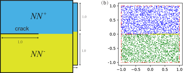
(a)

Figure 5: The schematic diagram of III mode crack: (a) NN⁺ represents the neural network in the upper area. NN^-represents the different neural network in the lower area. the geometric size is a square with side length 2, the length of the crack is 1, spanning in the middle of the structure , i.e., x<0, y=0. (b) Illustration of different sampling sizes and strategies, the blue points are the internal training points of the neural network $NN^{+}$, the green points are the internal training points of the neural network $NN^{-}$. The red points are the training points of the essential boundary conditions, and the yellow points are the interface points of the different neural network. The total number of internal points in the upper and lower regions is 4096, the number of essential boundaries condition points is 256, and the number of interface points is 1000. All points are randomly distributed unless otherwise stated.

Therefore, compared with CPINN, CENN requires additional construction of possible displacement fields that meet the essential boundary conditions. The RBF distance network and the particular network that meets the essential boundary conditions need to be constructed in advance. The number of RBF allocation points and the arrangement of points need to be determined according to the geometric shape of the essential boundary conditions. In this example, there are 121 uniform points in the domain as shown in Fig. 6a. RBF distance network prediction is shown in Fig. 6b. The average error of the RBF network is about 0.76 %. The accuracy can be improved by increasing the RBF center point including boundary points and the domain points, but it will increase the amount of calculation. After obtaining the RBF distance network, we train two particular networks in the upper and lower region to fit the essential boundary conditions. The hidden layer of the particular network has 3 layers, each layer has 10 neurons more shallow than the general network, the activation function is tanh in all the hidden layers, and an identical function is used in the output layer, the optimizer is Adam [42], the learning rate is 5e-4. It is worth noting that the neural network structure of the particular solution network does not need to be too complicated thanks to the powerful fitting ability of the neural network. A simple neural network structure can fit the essential boundary conditions well. It is worth noting that we must add $\mathcal{L}_{interface}=||u^{+}-u^{-}||$ at the interface to satisfy the continuity, and the convergence condition of the particular network training is that the MSE is less than 1e-6. Fig. 7a and b show that the output of the particular network is close to the pattern of the exact solution because the boundary conditions are all essential boundary conditions enclosing the interesting domain. As shown in Fig. 7c, the network structure can fit the boundary value well as the number of network training rounds increases. The loss function of the boundary drops a little faster than the loss value of the interface because there is a specific label at the boundary. The convergence speed of the boundary loss of different particular networks is almost the same, which shows that the particular network can learn the x-axis center symmetry of the exact solution very well. It does not matter that the particular network and the exact solution are quite different in the domain without essential boundaries. Because the function of the particular network is to precisely satisfy the given value at the essential boundary conditions. To further explore the performance of the particular network, we make a clockwise circle around the essential boundary as shown in Fig. 7d. Fig. 7e shows the comparison of the particular network and the exact solution at the essential boundary. We can find that the particular network can fit the essential boundary conditions very well, which is the result of the powerful fitting ability of the neural network.

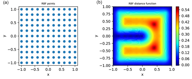
Figure 6: The RBF of III mode crack. (a) The RBF distance network of III mode of the crack: RBF points allocation map. (b) RBF distance network prediction contour.

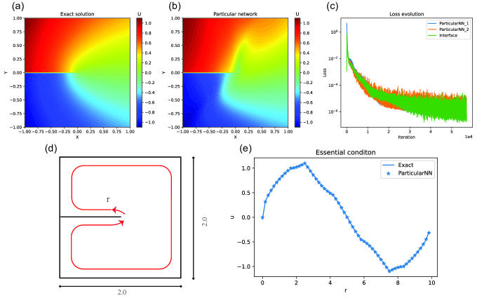
Figure 7: The particular neural network of III mode crack. (a) The contour of the exact solution of III mode crack. (b) The contour of the particular prediction. (c) Evolution of the MSE loss for training particular network, particularNN_1 and 2 represent the neural network satisfying the essential boundary condition of up and down region respectively. The number and the arrangement of points in both neural networks are same. Points are redistributed every 10 epoch. (d) The evaluation trace of the particular solution, starting from the center point and going around the boundary clockwise. (e) The comparison of the particular network and the exact solution on the trace of the boundary clockwisely

After constructing the possible displacement field, we compare data-driven, CPINN and CENN. The number of allocation points of these three ways is the same. The network structure and optimization scheme are also the same. It is worth noting that CPINN does not use the construction of the admissible function, but the other two methods (data-driven and CENN) do that. The generalized network has 4 layers, each layer has 20 neurons, and the learning rate is 1e-3. We consider the admissible function

$$\boldsymbol{u}(\boldsymbol{x})=\boldsymbol{u}_{p}(\boldsymbol{x};\boldsymbol{\theta}_{p})+RBF(\boldsymbol{x})\cdot\boldsymbol{u}_{g}(\boldsymbol{x};\boldsymbol{\theta}_{g})$$ (37)

where $\boldsymbol{u}_{p}$ is the particular network, $\boldsymbol{\theta}_{p}$ is the parameter of the particular network, RBF is the radial basis function, $\boldsymbol{u}_{g}$ is the generalized network, $\boldsymbol{\theta}_{g}$ is the parameter of the generalized network. In the training process, we freeze the parameters of the particular network and RBF, and only train the generalized neural network through the gradient descent method, i.e., Adam. It is worth noting that RBF is equal to zero at the essential boundary, so the role of the generalized network is eliminated, which results that the particular network only plays games. If the training of the RBF and particular network is successful, then the admissible function accurately meets the given displacement value at the essential boundary, which is the heart of the admissible function. On the other hand, the CPINN subdomains are the same as CENN, i.e., the upper and lower neural networks. The boundary conditions and the interface conditions are imposed by the penalty method, noting that the interface conditions include not only the continuous condition of displacement but also the continuous condition of displacement derivative, i.e.,

$$\begin{split}\boldsymbol{n}\cdot(\nabla u^{+}-\nabla u^{-})=0,&\boldsymbol{x}\subseteq\varGamma^{inter}\\ u^{+}(\boldsymbol{x})=u^{-}(\boldsymbol{x}),&\boldsymbol{x}\subseteq\varGamma^{inter}.\end{split}$$ (38)

Compared to CENN, one more loss is added, and the additional loss function is the derivative form, which will reduce the accuracy and efficiency. The loss function of CPINN is

$$\begin{split}\mathcal{L}&=\lambda_{1}\int_{\Omega^{+}}|\triangle(u^{+})|^{2}d\Omega+\lambda_{2}\int_{\Omega^{-}}|\triangle(u^{-})|^{2}d\Omega+\lambda_{3}\int_{\varGamma^{+}}|u^{+}-\bar{u}|^{2}d\varGamma+\lambda_{4}\int_{\varGamma^{-}}|u^{-}-\bar{u}|^{2}d\varGamma\\ &+\lambda_{5}\int_{interface}|u^{-}-u^{+}|^{2}d\varGamma+\lambda_{6}\int_{interface}|\boldsymbol{n}\cdot(\nabla u^{+}-\nabla u^{-})|^{2}d\varGamma\end{split}$$ (39)

It is not difficult to find that there are many hyperparameters in CPINN (more subdomains will further increase hyperparameters). Through tuning repeatedly, we have selected the best set of hyperparameters, $\lambda_{1}=\lambda_{2}=1,\lambda_{3}=\lambda_{4}=50,\lambda_{5}=\lambda_{6}=10$ (maybe there are better hyperparameters, because there are 6 hyperparameters, the workload of tuning parameters is very large). [30] shows that it is possible to use NTK (Neural tangent kernel) theory to automatically adjust hyperparameters for PINN, but there is no method for hyperparameter adjustments in the form of subdomain PINN, i.e., CPINN. Fig. 8a and e show the data-driven prediction results and absolute error, Fig. 9c shows that the overall relative error of the data-driven is 2.12 %. Due to the randomness of the initial parameters of the neural network, the initial parameters are initialized with Xavier [43], i.e. a method to initialize parameters. If not specified, all the results below are the average of 5 times. Since data-driven does not consider PDE, the loss function does not include auto differential [36], which has higher accuracy and computational efficiency. We found the absolute error near the center (x=0, y=0) is the largest as shown in Fig. 8d. Fig. 10a and b show that the exact solution is not smooth at the center. This is the reason for the large error at the center point. In addition, there were relatively sharp fluctuations at the beginning loss evolution, and then gradually converged. Fig. 8b and e shows that the prediction results of CPINN are sharp relatively, and the errors are also mainly concentrated in the center point. Because the derivative of analytical solution with respect to $\theta$ is singular at the center point, causing the loss at the center point to fluctuate sharply. Considering that CPINN and data-driven are both MSE errors, the optimal loss values both are 0, so we compare the loss functions of the two together as shown in Fig. 9a. In addition, CENN is based on the energy method, and the loss function is an energy functional, so the optimal loss value is not 0. From Fig. 9a, it can be seen that the CPINN loss function is higher than data-driven. The CPINN loss function is unstable compared to the data-driven, which is due to the high-order derivatives involved. In addition, the decreasing trend of the loss function of the different networks is similar in CPINN. The reason is the x-axis symmetry of the crack problem. To further analyze the performance of these three methods, we compare the relative error $L_{2}=\sqrt{\Sigma_{i=1}^{N_{pred}}error^{2}(\boldsymbol{x}_{i})}/\sqrt{\Sigma_{i=1}^{N_{pred}}exact^{2}(\boldsymbol{x}_{i})}$ in all three methods. We include the comparison of CENN and CPINN-RBF (CPINN: Boundary conditions are satisfied by penalty method, CPINN-RBF: Boundary conditions are satisfied by constructing the admissible function with RBF in advance). Fig. 9c shows that the overall relative error of CPINN is 3.61 %, and the overall relative error of CPINN-RBF is 7.31 %. This is one of the reasons that the weight of the different loss functions is not adjusted to the optimal value. In addition, CPINN involves higher-order derivatives, so the efficiency and accuracy are not as good as CENN. Fig. 8c and f show that the prediction result of CENN is smooth, not as sharp as CPINN. Fig. 9c shows that the overall relative error of CENN is 1.52 % and the overall result of CENN is more precise than CPINN and even better than data-driven accuracy. Due to the low derivative order of the loss function, the efficiency is higher than CPINN. The error distribution is more uniform. The main error is at the center point (x=0, y=0), which is caused by the form of the admissible function. This will be analyzed in the discussion part in Section 5 in detail. Fig. 9b shows that CENN loss function converges to the exact value of the functional

$$J=\int\frac{1}{2}\text{[}(\frac{\partial u}{\partial r})^{2}+(\frac{\partial u}{r\partial\theta})^{2}]rdrd\theta=\int[\frac{1}{8\sqrt{x^{2}+y^{2}}}]dxdy.$$

The analytic integration of the energy functional is about 0. 8814. According to the principle of minimum potential energy, the exact solution is the minimum value of the energy functional, i.e., 0.8814 in this problem. The reason for a small amount of fluctuation in the later stage of the training is due to the learning rate and the numerical integration accuracy, as shown in Fig. 9b. This can be eliminated by reducing the learning rate and adopting a more precise numerical integration scheme. In addition, the loss function is sometimes slightly lower than the exact value due to numerical integration and discrete errors, which can be reduced by increasing random points. Fig. 9c shows that CENN outperforms CPINN obviously, and even surpasses data-driven that does not involve coordinate derivatives. Finally, we can find that the trends of the loss function and relative error of the above three methods are the same.

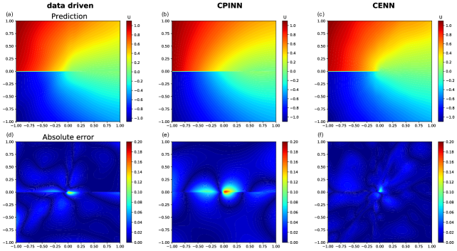
Figure 8: Purely date-driven model with mean square error (MSE) of displacement field: prediction (a) and absolute error (d). CPINN model with MSE loss function: prediction (b) and absolute error (e). CENN model with energy functional loss and $\lambda_{interface}=2700$: prediction (c) and absolute error (f).

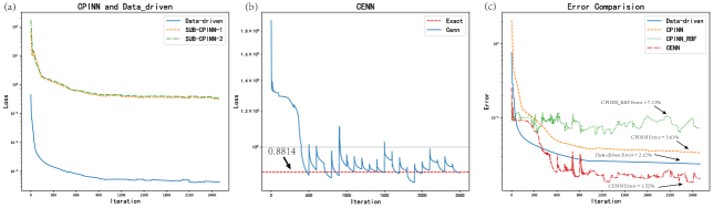
Figure 9: Comparison the loss and error of data-driven, CPINN and CENN in III mode crack: (a) Comparison of the CPINN loss value and data-driven loss value. SUB-CPINN-1 and 2 are CPINN subdomains NN in upper region and lower region of crack respectively. (b) Comparison of CENN energy functional and exact functional integration. (c) Comparison of the overall relative error $L_{2}$ of data driven, CPINN, CPINN-RBF and CENN.

Next, we compare the discontinuous displacement solutions and singular strains that we are more concerned about. Fig. 10 shows the comparison of solution of data-driven, CPINN and CENN at various x and y position. We observe the displacement of y=0, the up and down displacement. This is because at (x<0, y=0), the displacement solution is multiple values of the same coordinate, so there are two displacement solutions as shown in Fig. 10a,b. We take into account the strain

$$\varepsilon_{z\Theta}|_{interface}=\frac{1}{r}\frac{\partial u}{\partial\theta}=\frac{1}{2\sqrt{r}}cos(\frac{\theta}{2})|_{\theta=0}=\frac{1}{2\sqrt{r}},$$ (40)

the y-direction derivative of the displacement is singular at the center (x=0, y=0), so we research the singular strain at the interface, and explore whether the neural network is capable of fitting the singularity problem. Fig. 10a and b shows that the prediction of CENN and data-driven is close to the displacement solution, and both have higher accuracy than CPINN. The error between CENN and data-driven is large at x=0 caused by the RBF distance network of the admissible function, which will be further analyzed in Section 5. Fig. 10c shows the comparison of x=0. The accuracy of CENN at x=0 is higher than that of data-driven as the same as y=0, and the error near the center point is higher. It is also the reason that the RBF distance network of the admissible function causes. Fig. 10d shows the singular strain. The performance of CENN in singular strain is better than data-driven and CPINN. This is because loss function of CENN is constructed based on the physical minimum energy theory whose interpretability is stronger. The strain will cause the loss function to change in CENN, which will make the CENN strain converge to the exact solution. In numerical methods such as finite element, the singular point of fracture mechanics often requires a special quarter-node element [4], but this method does not have a special treatment, which comes from the tremendous function space of the neural network itself.

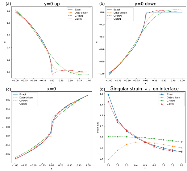
Figure 10: Different location comparison among data-driven, CPINN, and CENN: (a) Comparison of the displacement solution on the horizontal line y=0 up. (b) Comparison of the displacement solution on the horizontal line y=0 down. (c) Comparison of displacement solution at x=0. (d) Comparison of singular displacement derivative ${\partial u}/{\partial y}$ ($\varepsilon_{z\Theta}$) at x>0, y=0.

4.2 Non homogeneous problem with complex boundary

In this section, we investigate the problem with the complex boundary to shows the proposed method CENN can tackle the complex boundary and heterogeneous problem. Complex boundary problem can not be solved well in a traditional method such as FEM [2]. So we consider the Koch snowflake (complex boundary problem) as our boundary. We also solve the non-homogeneous problem, which is widespread in physics such as composites material, as shown in Fig. 11a, the fractal level L=2. The govern equation of the problem is [24]

$$\begin{cases}-a(\boldsymbol{x})\triangle u(\boldsymbol{x})=f(\boldsymbol{x})&\boldsymbol{x}\in\Omega\\ u(\boldsymbol{x})=g(\boldsymbol{x})&\boldsymbol{x}\in\partial\Omega,\end{cases}$$ (41)

where $\alpha(x)=\alpha_{i},x\in V_{i}$, $\alpha$ for different regions is a different constant. For the sake of simplicity, we consider

$$\begin{cases}a_{1}=\frac{1}{15}&r<r_{0}\\ a_{2}=1&r\geq r_{0}.\end{cases}$$ (42)

We adopt the exact solution

$$u(r,\theta)=\begin{cases}\frac{r^{4}}{\alpha_{1}}&r<r_{0}\\ \frac{r^{4}}{\alpha_{2}}+r_{0}^{4}(\frac{1}{\alpha_{1}}-\frac{1}{\alpha_{2}})&r\geq r_{0}.\end{cases}$$ (43)

The energy form of the problem is

$$J=\int_{\Omega_{1}}\frac{1}{2}\alpha_{i}(\nabla u)\cdot(\nabla u)d\Omega+\int_{\Omega_{2}}\frac{1}{2}\alpha_{i}(\nabla u)\cdot(\nabla u)d\Omega-\int_{\Omega}fud\Omega.$$ (44)

where $\Omega_{1}$ is the domain $r<r_{0}$ and $\Omega_{2}$ is the domain $r\geq r_{0}$ , $r_{0}=0.5$. It is worth noting that the exact solution is $C_{0}$, but $\partial u/\partial r$ is discontinuous on the interface.

The RBF distance network is shown in Fig. 11b and c, which has more collocation points than the crack problem due to the complex boundary conditions. We can find the prediction of the RBF distance network matches the accurate distance.

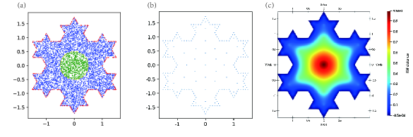
Figure 11: Distance network with complex boundaries of inhomogeneity: (a) Illustration of different sampling size and points allocation strategy, the green points are the PDEs parameter $a=$$1/15$($r<0.5$) training points, the blue points are the $a=1$($r>0.5$) training points, the red points are the training points of the essential boundary conditions, and the yellow points are the interface points ($r=0.5$) of the different domain, the total number of domain points is 10000, the number of essential boundary condition points is 4800, and the number of interface points is 1000. All points are randomly distributed. (b) The collocation point diagram of RBF network, uniform distribution, 217 points on the boundary, 48 points in the domain. (c) Prediction of RBF distance network.

The convergence condition of the particular network training is that the MSE is less than 1e-6. The hidden layer of the particular network has 4 layers, each layer has 20 neurons, the activation function is tanh in all hidden layers, and an identical function is used in the output layer, the optimizer is adam, the learning rate is 5e-4. Fig. 12 shows the particular pattern is close to to the pattern of the exact solution, because the essential boundaries enclose the domain. The loss function value of the particular neural network decreases as the number of iterations increases, which shows the particular network can fit the essential boundary accurately. The oscillation of the loss is the reason that the learning rate is not adequate small, we can decrease the learning rate as iterations increase to eliminate the oscillation phenomenon.

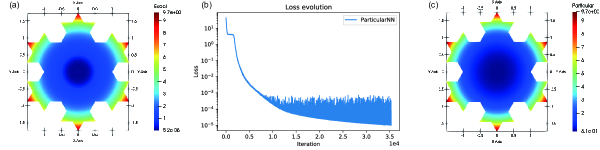
Figure 12: Koch particular neural network: (a) The contour of the exact solution of Koch. (b) The evolution of the MSE loss for the training particular network. (c) The contour of the prediction of the particular network.

Given that the derivative on the interface is discontinuous, we compare CPINN, DEM, and CENN. We divide the domain into 2 subdomains, i.e., $r=0.5$ as the partition , considering the derivative discontinuity on the interface. The neural network architecture is the same in the both subdomain, which can be also different. The hidden layer of the particular network has 4 layers, each layer has 20 neurons. The activation function is tanh in all hidden layers, and identical function is used in the output layer. Adam is used as the optimizer, and the learning rate is 1e-3. The training points are randomly distributed in all methods as shown in Fig. 11a. Training points are redistributed every 100 epochs for all three methods. The penalties $\lambda$ of every loss function in CPINN are : $\lambda_{1}=60$ when $r<r_{0}$, $\lambda_{2}=1$ when $r>r_{0}$, $\lambda_{inter}$=1 when $r=r_{0}$, $\lambda_{bound}=30$ on the essential boundary (We adjusted a lot of penalties $\lambda$, this is the best set). It is worth noting that the loss of CPINN on the interface includes

$$\begin{cases}u^{+}=u^{-}\\ a_{1}(\boldsymbol{n}\cdot\nabla u^{+})=a_{2}(\boldsymbol{n}\cdot\nabla u^{-})\end{cases}$$ (45)

where $u^{+}$ and $u^{-}$ represent the internal and external region neural network respectively. For the sake of simplicity, the two interface loss terms are controlled by the same penalty $\lambda_{inter}$. We adopt sequential training for two neural networks [18]. In particular, we first optimize $u^{+}$ parameters with $u^{-}$ parameters fixed for 20 epochs, then vice versa in CPINN. DEM and CENN are trained by the admissible function. CENN is trained by sequential training to pay attention to the internal energy (internal), given that the difference between the energy of internal and external is too large. we first optimize $u^{+}$ parameters with $u^{-}$parameters fixed for 2500 epoch in CENN, then vice versa. We use the admissible function in the external region, while not in the internal region because the whole boundary condition is in the external region boundary. We stitch the subdomains through the interface loss.

Fig. 13 shows the prediction and absolute error of these three methods. The maximum absolute error of CPINN is on the boundary because the second-order derivation of the solution is big on the boundary in CPINN, resulting in the prediction sensitivity on the boundary. The error of DEM is mainly in the middle of the region($r<r_{0}$), because the energy density $\frac{1}{2}\alpha_{1}(\nabla u)\cdot(\nabla u)=8r^{6}/a_{1}$ is much smaller than the external energy density. The big difference in internal and external energies results in paying too much attention to the external region. The maximum absolute error in CENN, CPINN, CENN is 0.34, 0.74, and 0.11 respectively. The error in the CENN is mainly concentrated in the area near the center point, which is obviously smaller than DEM in terms of error magnitude and range. In CENN, because the energy density $\frac{1}{2}\alpha_{1}(\nabla u)\cdot(\nabla u)=8r^{6}/a_{1}$ is close to zero when $r$ is close to the center point, the loss of the internal will pay attention to the region where the loss can be decreased faster, resulting in the error in the center point.

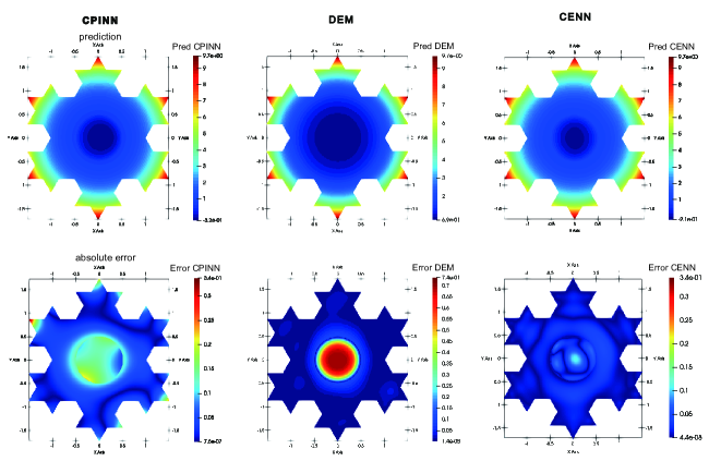
Figure 13: Prediction and absolute error by CPINN, DEM, and CENN in Koch: The displacement field prediction result (a,b,c), absolute error (d,e,f).

To further analyze the performance of these three methods, we compare the loss and relative error $L_{2}$. Considering that the loss of DEM and CENN are both energy variational, so the optimal values both are the same, so we compare the loss functions of these two methods together as shown in Fig. 14. Due to the complexity of the boundary conditions, we calculate the exact numerical integral for this case by the Monte Carlo algorithm. The exact values of the internal and the external are 1.10 and 436.45 respectively. To better visualize it, we normalize the energy loss. Fig. 14a shows the trend of the different part loss evolution in CPINN are similar, which proves our choice of the penalty is relatively good. Fig. 14b shows DEM can not converge to the exact internal energy, which is the reason why the absolute error in the internal region is obviously large than the external region. However, CENN can converge to the exact internal energy well due to the subdomains. Fig. 14c shows CENN and DEM both converge to the external energy because the external energy dominates the majority of the total energy. The fluctuation in the external and internal energy can be eliminated by decreasing the learning rate. Fig. 14d shows the relative error $L_{2}$ is 2.6%, 1.02%, 6.9%, and 0.81% in CPINN, CPINN-RBF, DEM, and CENN respectively. We find that CPINN-RBF improves the performance against CPINN except in the first numerical experiment (crack). It may be that the penalty factor in the first numerical example is more suitable than admissible function. Obviously , CENN can solve the composite problem very well, and there is only one hyperparameter penalty about the interface in the loss function. Finally, we can find that the trends of the loss function and relative error of the above three methods are the same.

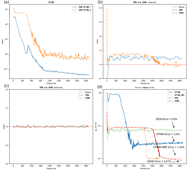
Figure 14: Comparison of CPINN, DEM, and CENN in Koch: (a) The loss function evolution of CPINN. SUB-CPINN-1 and 2 are CPINN subdomains NN in the internal and external regions respectively. (b) Comparison of DEM and the CENN loss function in the internal region with exact normalized internal functional integration. (c) Comparison of DEM and the CENN loss function in the external region with exact normalized functional integration. (d) Comparison of CPINN, CPINN-RBF, DEM, and CENN $L_{2}$ error.

To further analyze the interface prediction of these three methods, we compare the solution and the discontinuous derivative on the interface. Fig. 15a and b show the comparison of solution of CPINN, DEM and CENN at two cross lines, x=0 and y=0. CENN is more accurate than other methods in predicting solutions, and the error increases slightly near the center area, the reason may be relatively little energy density in the center point. The center error may be alleviated by adopting more points in the internal region, which we will further study in the future. It is worth noting that the derivative solution by CPINN is more accurate than CENN and energy method, as shown in Fig. 15c,d. The reason may be the second-order derivative used in CPINN is not smaller than the first-order derivative in CENN in the internal region, so the derivative in the internal region can be trained well by strong form. It is worth noting the solution prediction of these three methods is smaller than the exact solution, which is suitable for some engineering conservative problems.

Given that the strong form of PINN can adopt batch strategy, it is very useful to improve the efficiency of network training. However, because CENN is a deep energy method, the precise numerical integration of energy functional is very important. So we use as many integration points as possible in CENN. In order to compare the computational efficiency of CPINN and CENN, we compare CENN with CPINN under different batch sizes. Table 1 shows that the efficiency and accuracy of CENN are better than CPINN in the same batch size 10000. The error and time in Table 1 are the results after the network converges. We can find that different batch sizes of CPINN have a significant impact on the accuracy of the solution, which is mainly due to the high randomness of the training points and the strong non-convex property of the loss function. It is worth noting that the efficiency of CENN in solving high-order tensors and high-order PDEs will be greater than that of CPINN (the problem of crack is second-order and scalar PDEs, so the efficiency advantage of CENN is not very obvious ).

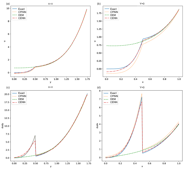
Figure 15: Different location comparison of CPINN, DEM, and CENN in the Koch: (a) Comparison of the displacement solution on the vertical line x=0. (b) Comparison of the displacement solution on the horizontal line y=0. (c) Comparison of the displacement derivative ${\partial u}/{\partial r}$ on the vertical line x=0. (d) Comparison of the displacement derivative ${\partial u}/{\partial r}$ on the horizontal line y=0.

Table 1: Compare the training time of CPINN and CENN. The network structure is exactly the same. Batch size refers to the random number of points required for each epoch of CPINN, and each epoch is randomly scattered. CENN takes as many integration points as possible because of the accuracy requirement of energy numerical integration. $L_{2}$ error and time are the results of convergence.

	Batch size	$\mathcal{L}_{2}$ error	Time (s)
	100	7.1%	62.45
	500	6.9%	66.15
CPINN	1000	2.5%	71.25
	3000	3.1%	176.25
	5000	3.4%	148.2
	10000	2.6%	247.8
CENN (Whole Batch)	10000	0.81%	176.4

4.3 Composite material hyperelasticity

In this section, we introduce hyperelasticity, which is a well-known problem including non-linear operator and vector-valued variables in solid mechanics. In [25], the homogeneous hyperelasticity problem is solved. We consider a body made of a nonhomogenous material to show the proposed method CENN can tackle the non-linear and heterogeneous problem, i.e., composite hyperelastic material. The non-linear characteristic is from the large deformation and the hyperelastic constitutive law. The governing equation of the problem is

$$\begin{cases}\nabla_{X}\cdot\boldsymbol{P}+\boldsymbol{f}=0&\boldsymbol{x}\in\Omega\\ \boldsymbol{u}=\bar{\boldsymbol{u}}&\boldsymbol{x}\in\partial\Omega^{eb}\\ \boldsymbol{N}\cdot\boldsymbol{P}=\bar{\boldsymbol{t}}&\boldsymbol{x}\in\partial\Omega^{nb}\end{cases}$$ (46)

where $\nabla_{X}$ is the gradient operator with respect to $\boldsymbol{X}$, $\boldsymbol{X}$ is material coordinate [44]. $\nabla_{X}\cdot\boldsymbol{P}$ denotes the divergence operator, and we can use the tensor index to represent clearly $\nabla_{X}\cdot\boldsymbol{P}=P_{ij,i}$. $\boldsymbol{P}$ is the Lagranges’s stress, where the first component $i$ and the second $j$ of $P_{ij}$ correspond the material coordinates and spatial coordinate respectively. $\boldsymbol{f}$ is the body force, and the first equation is the equilibrium equation in the domain $\Omega$. Note that $\boldsymbol{P}$ is the function of the material coordinate $\boldsymbol{X}$. $\bar{\boldsymbol{u}}$ is the given displacement value in the essential boundary $\partial\Omega^{eb}$. $N$ is the normal direction of the Newmann boundary $\partial\Omega^{nb}$, and $\bar{\boldsymbol{t}}$ is the prescribed traction on the Newmann boundary.

If the material is hyperelasticity, then $\boldsymbol{P}$ can be written to be the derivative of the strain energy $\Psi$ with respect to the deformation gradient $\boldsymbol{F}$

$$\boldsymbol{P}=(\frac{\partial\Psi}{\partial\boldsymbol{F}})^{T}$$ (47)

$$\boldsymbol{F}=\frac{\partial\boldsymbol{x}}{\partial\boldsymbol{X}}$$ (48)

where the $\boldsymbol{x}=\boldsymbol{X}+\boldsymbol{u}(\boldsymbol{X})$ is the spatial coordinate, which is the function of the material coordinate $\boldsymbol{X}$, given that it is a static problem independent of time. $\boldsymbol{u}$ is the interesting field, which in this specific problem is the vector displacement field. We consider the common used constitutive law Neo-Hookean of the hyperelasticity [45]

$$\varPsi=\frac{1}{2}\lambda(lnJ)^{2}-\mu ln(J)+\frac{1}{2}\mu(trace(\boldsymbol{C})-3)$$ (49)

where $J$ is the determinant of the deformation gradient $\boldsymbol{F}$ and $\boldsymbol{C}$ is the Green tensor, i.e., $\boldsymbol{C}=\boldsymbol{F}^{T}\cdot\boldsymbol{F}$. The first and second terms of RHS respectively are uncompressible condition and stress-free in the initial condition. $\lambda$ and $\mu$ is Lame parameter

$$\begin{cases}\lambda=\frac{vE}{(1+v)(1-2v)}\\ \mu=\frac{E}{2(1+v)}\end{cases}$$ (50)

where $E$ and $v$ represent the elastic modulus and Poisson ratio respectively. The core of the problem is to obtain the displacement field $\boldsymbol{u}$. There are two ways to do it. The first way is to solve the strong form Equation 46 and the second way is to use the energy theory by optimizing the potential energy

$$\mathcal{L}=\int_{\Omega}(\Psi-\boldsymbol{f}\cdot\boldsymbol{u})dV-\int_{\partial\Omega^{nb}}\bar{\boldsymbol{t}}\cdot\boldsymbol{u}dA$$ (51)

Noting that the trial function satisfies the essential boundary in advance. In B, we can find the implementation of strong form is more complicated than the energy form, and the highest derivative of the strong form is higher than the energy form (The best hyperparameter combination of different PDEs and boundary conditions in CPINN is not known), which results in more computation cost and lower accuracy. For the sake of simplicity, we compare DEM and CENN. We use the FEM as the reference solution.

We consider a two-dimensional bending beam made of the composite material, as shown in Fig. 16. The material parameter is, upper : $E_{0}=1000,\mu_{0}=0.3$, lower : $E_{1}=10000,\mu_{0}=0.3$. FEM divides the region into 400 (length)*100 (height) quadratic elements for enough accurate reference solution. Fig. 16 shows the points distribution ways of the DEM and CENN. Training points are redistributed every 100 epochs in all methods. Because the given value on the essential boundary is zero, the particular neural network is zero, i.e., $\boldsymbol{u}_{p}=0$. In addition, given that the essential boundary geometry is simple, we can obtain the analytic solution of the distance function, i.e., $RBF(x,y)=x$ to ensure that the boundary conditions are exactly satisfied (RBF method can also be used here, but it is not necessary due to the simplicity of the boundary). The structure of the generalized network is 4 layers, each layer has 20 neurons, and the learning rate is 1e-3. We use LBFGS [46] as the optimizer. Given that the strain energy does not vary much from region to region, we optimize both neural networks in CENN not like the Koch example before. The neural network structure of DEM is same as CENN for comparison. Fig. 17 shows the prediction of the FEM, DEM, and the CENN. We can find that the minimum displacement x and y of the CENN is more close to the reference solution, i.e. FEM. The pattern of DEM and CENN both coincides with FEM. This shows the prediction of DEM and CENN about original field $\boldsymbol{u}$ is both good overall. To further quantify the error, we consider the relative error about displacement and Von-Mises stress related to the derivative of the displacement

$$Mises=\sqrt{\frac{3}{2}\boldsymbol{S}^{dev}:\boldsymbol{S}^{dev}}$$ (52)

where $\boldsymbol{S}$ is the Kirchhoff’s stress

$$\boldsymbol{S}=\boldsymbol{P}\cdot\boldsymbol{F}^{-T}.$$ (53)

and $\boldsymbol{S}^{dev}$ is the deviation tensor, i.e.,

$$\boldsymbol{S}^{dev}=\boldsymbol{S}-\frac{1}{3}trace(\boldsymbol{S})\boldsymbol{I}$$ (54)

Because of the different material parameters of the beam, the derivative of the displacement y with respect to the y-direction is discontinuous on the interface. This is also the case with the Von-Mises on the interface, so we consider the error $abs(\|Von^{pred}\|_{2}-\|Von^{fem}\|_{2})/\|Von^{fem}\|_{2}$ to consider the derivative error. Fig. 18a shows the loss evolution of the CENN is much lower than the CENN. It is worth noting the optimal loss of the energy method is not zero due to the minimal potential theory. In some ways, the loss can reflect the accuracy of the method. Fig. 18b shows the relative error of CENN about displacement magnitude is 1.3%, which is lower than DEM. Because $\partial u/\partial y$ is not continuity, it is natural to divide the region according to the different materials to ease the restriction of derivative continuity. Fig. 18c shows the relative error of CENN in Von-Mises stress is 0.11%, which is very much smaller than DEM. Because CENN can fit better the derivative on the interface due to the inherent ability to simulate the discontinuity, the prediction about Von-Mises in CENN is more close to the reference solution.

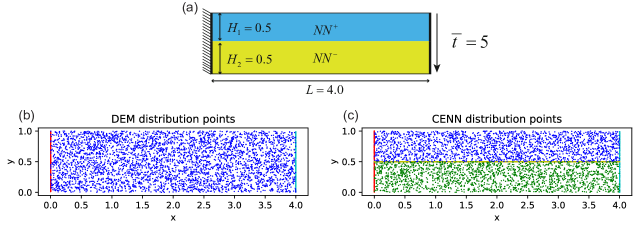
Figure 16: The schematic diagram of the composite material beam, the blue and yellow stack denotes the different hyperelastic material (up: $E_{0}=1000,\mu_{0}=0.3$; down: $E_{1}=10000,\mu_{0}=0.3$), we use different neural networks corresponding to the different material. The length of the beam is 4 and the height of the beam is 1, the downward traction acting the right end of the beam is 5N and the left end of the beam is an essential fixed boundary (a). Illustration of distribution points strategy of the DEM (b) and CENN (c), In DEM, the blue points are the domain training points of the neural network. In CENN, The blue points are the upper material training points of the neural network $NN^{+}$, the green points are the lower material training points of the neural network $NN^{-}$, the red points are the points of the essential boundary, and the yellow points are the interface points of the different materials. In both two energy ways, the total number of internal points is both 4096, the number of essential boundary points is both 256, and the number of interface points is both 1000. All points are randomly distributed (b,c)

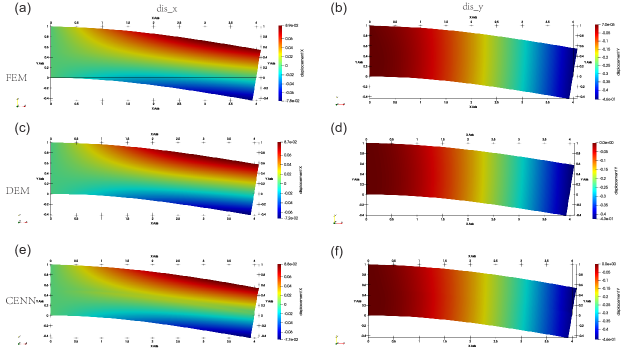
Figure 17: Predicted solution by FEM, DEM, and CENN in beam: The displacement X field prediction result (a,c,e), the displacement Y field prediction result (b,d,f), FEM predition (a,b), DEM predition (c,d), CENN predition (e,f).

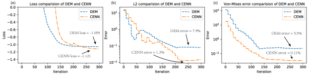
Figure 18: Comparison of DEM and CENN in beam: (a) The loss function evolution. (b) The relative error $L_{2}$ about displacement magnitude. (c) The relative error about Von-Mises stress.

To further analyze the interface prediction of DEM and CENN, we compare the discontinuous derivative on the different vertical lines cross the interface, x=1, x=2, and x=3, and we also compare the main deformation, i.e. $u_{y}$, on the different horizontal line, y=0.25, y=0.5 and y=0.75. Fig. 19a,b,c show the comparison of Von-Mises of DEM and CENN on the different vertical lines cross the interface, x=1, x=2, and x=3. We can find CENN is more accurate than DEM in terms of discontinuous derivative. Fig. 19d,e,f show the comparison of displacement y of DEM and CENN on the different horizontal lines, y=0.25, y=0.5, and y=0.75. We can find both methods are good overall in terms of displacement y, but CENN is better.

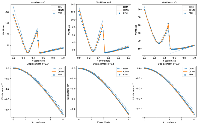
Figure 19: Different location comparison of DEM and CENN in beam: Comparison of the Von-Mises solution on the different vertical line, x=1, x=2, x=3 respectively (a,b,c), comparison of the displacement y solution on the different horizontal line, y=0.25, y=0.5, x=0.75 respectively (d,e,f).

5 Discussion

5.1 Discussion of admissible function errors

The above-mentioned data-driven and CENN error at the center point (crack problem) is larger than other points. Here we analyze the reason. We consider the derivative of the ring direction $\theta$ at the center point.

$$\frac{\partial u(r,\theta;\boldsymbol{\theta}_{p},\boldsymbol{\theta}_{g})}{r\partial\theta}=\frac{\partial u_{p}(r,\theta;\boldsymbol{\theta}_{p})}{r\partial\theta}+\frac{\partial RBF(r,\theta)}{r\partial\theta}\cdot u_{g}(r,\theta;\boldsymbol{\theta}_{g})+RBF(r,\theta)\cdot\frac{\partial u_{g}(r,\theta;\boldsymbol{\theta}_{g})}{r\partial\theta}$$ (55)

Here we assume that the RBF distance network is correct. It can be found in Fig. 6b , the result of the RBF distance network is consistent with the analytical solution. Therefore, this assumption is reasonable. Obviously, the RBF distance network in the Equation 55 is equal to zero at the center point. At the same time, the RBF distance network keeps the same distance from the center point on the right half, as shown in Fig. 20, i.e., $\partial RBF(r,\theta)/r\partial\theta=0$. So when approaching the center point, $\partial RBF(r,\theta)/r\partial\theta$ and $RBF(r,\theta)$ are both zero, which will cause $\partial u(r,\theta)/r\partial\theta=\partial u_{p}(r,\theta)/r\partial\theta$. However we fixed the parameters of the particular network during training, so the energy density $J_{\rho}=\frac{1}{2}[(\partial u/\partial r)^{2}+(\partial u/r\partial\theta)^{2}]$ at the center point can not be trained completely, i.e., $\partial u/r\partial\theta$ does not change, which leads to a large error at the center. Fig. 8e and f show that the error is mainly concentrated in the right half of the center point. This shortcoming can be overcomed by changing the derivative term of the RBF distance network, i.e., change the form of the distance network to make $\partial RBF(r,\theta)/r\partial\theta\neq 0$ at the center point. It will make training of the generalized network useful to perform learning further in the center. In another way, we can retrain the parameters of the particular network, but we need to add an additional penalty function to limit the change of the particular network parameters so that the energy density at the center point can be changed. This problem will be further studied in the future.

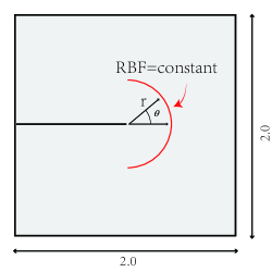
Figure 20: RBF distance network constant diagram, r and $\theta$ are standard polar coordinates, the prediction of RBF distance network is constant in the right half when $r=constant$, and the red line is the position where RBF prediction is constant

We consider the singular strain at x>0, y=0. Fig. 10d shows that the error will increase when approaching x=0. This is actually a special case of the above-mentioned hoop $\theta$ derivative situation at the interface (x>0, y=0), $\partial u(r,\theta)/r\partial\theta=\partial u(x\text{,}y)/\partial y$. It is also caused by the RBF distance network of the addmissible function, we consider the derivative $u$ w.r.t y-direction at the center point

$$\frac{\partial u(x\text{,}y;\theta_{p},\theta_{g})}{\partial y}=\frac{\partial u_{p}(x,y;\theta_{p})}{\partial y}+\frac{\partial RBF(x,y)}{\partial y}\cdot u_{g}(x,y;\theta_{g})+RBF(x,y)\cdot\frac{\partial u_{g}(x,y;\theta_{g})}{\partial y}.$$ (56)

Obviously, the RBF distance network in Equation 56 is equal to zero at the center point. In addition, we analyze $x=\delta$, y=0 at $\partial RBF(x,y)/\partial y$, Taylor series expand to second-order term

$$\begin{split}\frac{\partial R(y)}{\partial y}&=lim_{d\rightarrow 0}\frac{\sqrt{\delta^{2}+d^{2}}-\delta}{d}\\ &=lim_{d\rightarrow 0}\frac{(\sqrt{\delta^{2}}+\frac{\partial(\sqrt{\delta^{2}+d^{2}})}{\partial y}|_{d=0}d+\frac{1}{2}\frac{\partial^{2}(\sqrt{\delta^{2}+d^{2}})}{\partial^{2}y}|_{\triangle=0}d^{2}+o(d^{2}))-\delta}{d}\\ &=lim_{d\rightarrow 0}\frac{(\sqrt{\delta^{2}}+\frac{1}{2}\frac{1}{\delta}d^{2}+o(d^{2}))-\delta}{d}\\ &=0\end{split}$$ (57)

Where $\delta$ is the distance from the center point (crack tip), $\delta>0$, the coordinate point is $(x=\delta,y=0)$, where $d$ is the distance from the coordinate point to the x-axis, it is not difficult to find that the above derivative is always equal to 0 at $x>0,y=0$. So when approaching to the center point, $\partial R(x,y)/\partial y=R(x,y)=0$, which will lead to $\partial u(x\text{,}y)/\partial y=\partial u_{p}(x,y)/\partial y$. However, we fixed the parameters of the particular network during training, so the closer is to the center point, the more sensitive generalized network is. It will increase the error of $\partial u(x\text{,}y)/\partial y$ when approaching a center point.

5.2 The influence of point distribution on the solution

Different point allocation methods may affect the accuracy. At the same time, due to the constant of the distance network near the essential boundary, the generalized neural network near the essential boundary partially is very sensitive, resulting in increasing error. The sensitivity can be reduced by arranging more points around the center point.

The energy form depends more on the integration scheme because the loss function is the value of the energy functional. The different ways of attribution points have a relatively large impact on the energy form. However, the strong form requires the error at the sampling point to be 0, so the requirement for the integration scheme is not high. It is worth noting that the overall loss function tends to be 0 in strong form, so the gradient descent has an impact to all the sampling points. In a way, the attribution ways have also an impact on the strong form. The impact of the attribution ways on the energy form is shown explicitly, while the impact of the attribution ways on the strong form is implicit.

5.3 Efficiency and accuracy

Since the addmissible function requires additional training, the advanced training of the RBF distance network and the particular network will increase the additional computational cost. However, the traditional strong form does not need it, but the traditional strong form involves a higher-order derivative than the energy form. Thus the computational cost of the strong form is larger than the energy form after the admissible function training. This is a question of balance. In addition, higher-order derivatives will not only further increase the amount of the computational cost, but also affect the accuracy theoretically. It is worth noting that not all PDEs have a corresponding energy form, so the generality of the energy form is not as good as the strong form. At the same time, the energy form requires more strict collocation methods due to the requirement for precise integration functionals, while the strong form does not have this restriction, and some batch methods can be used to improve convergence speed [22]. In addition, the choice of hyperparameters in traditional strong form is also a problem. Although there is NTK theory to automatically select hyperparameters [29, 30], accurate and quantitative optimal hyperparameters is still an important problem. Of course, the strong form can also use the construction of the addmissible function to reduce the number of hyperparameters. If multiple neural network subdomains are involved, the hyperparameters about the interface will further increase greatly, and the interface loss term in CPINN will add the derivative term compared to the CENN. It will reduce the accuracy and efficiency. It is worth noting that there is no NTK theory of subdomains to automatically determine the hyperparameters, which will be further studied in the future.

5.4 Use adaptive activation function to accelerate the convergence and improve the accuracy

There are some adaptive activation methods to accelerate the convergence and improve the accuracy [47, 48, 49]. The main motivation of the adaptive activation function is to increase the slope of the activation function [48]. The advantage of these methods is easy and useful, and we only add a few trainable parameters to the original neural network (the extra parameters are far less than the initial trainable parameters). We include LAAF[48] and Rowdy[47] to our initial CENN. LAAF adds extra trainable parameters in every layer of the neural network. The modification of LAAF compared to the origin neural network is

$$\sigma(na^{(l)}\boldsymbol{z}^{(l)})$$ (58)

, where untrainable n$\geq$ 1 is a pre-defined scaling factor to control the convergence speed of L_LAAF and the parameter trainable $a$ acts as a slope of activation function. The loss term $\mathcal{L}_{a}$ about the $a$ need to be added to the loss function,

$$\mathcal{L}_{LAAF} =\mathcal{L}_{initial}+\lambda_{a}\mathcal{L}_{a}$$ (59)

$$\mathcal{L}_{a} =\frac{D}{\sum_{k=1}^{D}exp(a^{(k)})}$$

, where $D$ is the number of the hidden layers (not including input and output layers). The meaning of $\mathcal{L}_{a}$ is the reciprocal of the mean $exp(a^{(k)})$ in every hidden layer. $\lambda_{a}$ is the weight of $\mathcal{L}_{a}$, we adopt $\lambda_{a}=1$. The detail of the L_LAAF is in [48].

Rowdy activation function is the special form of the Deep Kronecker neural networks (A general framework for neural networks with adaptive activation functions), which is demonstrated good performance in some numerical experiments [47, 48, 49]. The modification of Rowdy compared to the origin neural network is

$$\sum_{k=1}^{K}c_{k}^{(l)}\sigma_{k}(a_{k}^{(l)}\boldsymbol{z}^{(l)})$$ (60)

, where $c_{k}^{(l)}$ and $a_{k}^{(l)}$ are the trainable parameters in every hidden layer (the number of these is $2KD$). K is the different activation function. The Rowdy activation function which is a special different activation function is

$$\sigma_{k}(x)=nsin((k-1)nx)$$ (61)

where n $\geq$ 1 is the fixed positive number acting as a scaling factor. The detail of the Rowdy activation function is in [47].

We test LAAF and Rowdy3 in our first numerical example (crack), to examine the performance of the adaptive activation function in CENN. There are 3 different activation functions in Rowdy3,

$$\sigma_{1}(x) =tanh(x)$$ (62)

$$\sigma_{2}(x) =sin(x)$$

$$\sigma_{3}(x) =sin(2x)$$

K=3, n=1 in Rowdy. n=10 in L_LAAF. The architecture of the neural network is the same as the Section 4.1. The initialization of $a^{(l)}$ is 0.1 in all hidden layers in L_LAAF. The initialization of $c_{k}^{(l)}$ is $\left[\begin{array}[]{cccc}1&0&\cdots&0\end{array}\right]_{k*1}^{(l)}$ in every hidden layer. The initialization of $a_{k}^{(l)}$ is $\left[\begin{array}[]{cccc}1&1&\cdots&1\end{array}\right]_{k*1}^{(l)}$ in every hidden layer. Fig. 21 shows CENN with Rowdy3 can accelerate the convergence and improve the accuracy compared to the initial CENN without adaptive activation function. However, the CENN with L_LAAF does not improve accuracy and convergence speed. The easy numerical example shows that we can use the adaptive activation function to accelerate convergence and improve accuracy in CENN.

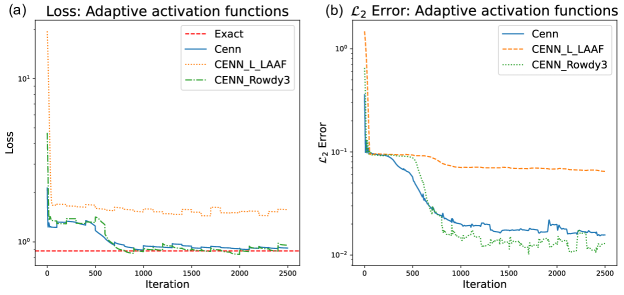
Figure 21: The performace of the adaptive activation function in crack example: Comparison of CENN, CENN with L_LAAF, and CENN with Rowdy3. (a) Loss function (b) Total relative $\mathcal{L}_{2}$ error.

5.5 Whether the generalized neural network is slicing

Considering that the interface is a continuous derivative in the crack, we do not actually need to slice the generalized network. But in some $C_{0}$ problems (the original function is continuous, the first derivative is discontinuous), e.g. heterogeneous problem, the slicing of the generalized network is meaningful, which has been specifically illustrated in Section 4.2 and Section 4.3.

We should consider the physical nature of the problem, then decide whether to slice the neural network or not. The different regions are connected through the interface loss function.

6 Conclusion

We developed the CENN formulation based on the deep energy method to solve the heterogeneous PDEs. We showed the accuracy of the proposed method is higher than the DEM in terms of the heterogeneous problem, especially the derivative on the interface. We show the efficiency and accuracy of the proposed method CENN compared to the CPINN due to the lower-order derivative. The hyperparameter of the proposed method is far less than CPINN. We show CENN can solve the singularity strain problem, i.e. crack, without special treatment such as finite crack element. We demonstrate why the PDE solution that uses neural networks as approximation functions can be successful from the perspective of trial functions as well as test functions. We proposed a method to construct the admissible function to solve the complex boundary problem, which extends the application range of the deep energy method. Further, we explore the ability of the proposed method to solve the hyperelasticity problem with heterogeneous material, high-order multi-physics, and vector-valued variables in solid mechanics. We show the ease of implementation of CENN compared to CPINN. We recommend the CENN if the heterogeneous PDE has the corresponding variational form because the accuracy and efficiency are better than CPINN and DEM.

Each region can be set individually in CENN, such as neural network structure, optimization method, this flexibility is a double-edged sword, the advantage is the freedom of choice, the disadvantage is that there is no optimal solution. A limitation of the proposed method is that the derivative w.r.t some direction on the essential boundary can not be learned well, which we will further study in the future. A limitation of this study is that the penalty of the interface is constructed by a heuristic algorithm, so the accurate quantity of the hyperparameter should be further studied in the future. CENN is based on the principle of the minimum potential energy, so it only can solve the static problem. In the future, we will research the Hamilton principle to solve the dynamic problem in PINN energy form. An additional uncontrolled factor in almost scientific computation based deep learning is how to choose initial parameters, optimization way, neural network architecture, and so on. It is worth emphasizing that the method has a natural advantage in dealing with heterogeneous problems.

Appendix A Back propogation of CENN

We consider the energy form of CENN

$$\begin{split}\mathcal{L}&=\sum_{i=1}^{n_{1}}w_{i}w_{\varepsilon}(u_{1}(\boldsymbol{x}_{i};\theta_{1}))-\sum_{i=1}^{n_{1}}w_{i}f_{i}u_{1}(\boldsymbol{x}_{i};\theta_{1})\\ &+\sum_{i=1}^{n_{2}}w_{i}w_{\varepsilon}(u_{2}(\boldsymbol{x}_{i};\theta_{2}))-\sum_{i=1}^{n_{2}}w_{i}f_{i}u_{2}(\boldsymbol{x}_{i};\theta_{2})\\ &+\frac{penalty}{n_{inter}}\sum_{i=1}^{n_{inter}}(u_{1}(\boldsymbol{x}_{i};\theta_{1})-u_{2}(\boldsymbol{x}_{j};\theta_{2}))^{2},\end{split}$$ (63)

where $w_{i}$ is the weight of the attribution points $x_{i}$, especially $w_{i}=V/n$ if uniform random Monte Carlo method is adopted. $w_{\varepsilon}$ is the strain energy density, $u_{1}$and $u_{2}$ are interesting variable according to the different subdomains. $f_{i}$ is the body force w.r.t. the point $x_{i}$. $\theta_{1}$and $\theta_{2}$ are neural network parameters according to the different subdomains. The last term on RHS is the continuity condition on the interface by the MSE criterion.

Back propagate Equation 63 to find the derivative of the loss function with respect to parameters of neural network 1

$$\begin{split}\frac{\partial\mathcal{L}}{\partial\theta_{1}}&=\sum_{i=1}^{n_{1}}w_{i}\frac{\partial w_{\varepsilon}(u_{1}(\boldsymbol{x}_{i};\theta_{1}))}{\partial u_{1}(x_{i};\theta_{1})}\frac{\partial u_{1}(\boldsymbol{x}_{i};\theta_{1})}{\partial\theta_{1}}-\sum_{i=1}^{n_{1}}w_{i}f_{i}\frac{\partial u_{1}(\boldsymbol{x}_{i};\theta_{1})}{\partial\theta_{1}}\\ &+\frac{penalty}{n_{inter}}\sum_{i=1}^{n_{inter}}2(u_{1}(\boldsymbol{x}_{i};\theta_{1})-u_{2}(\boldsymbol{x}_{j};\theta_{2}))\frac{\partial u_{1}(\boldsymbol{x}_{i};\theta_{1})}{\partial\theta_{1}}.\end{split}$$ (64)

If we consider the one dimension elastic problem, the strain energy density is

$$w_{\varepsilon}(u(\boldsymbol{x}_{i};\boldsymbol{\theta}))=\frac{1}{2}E(\frac{\partial u(\boldsymbol{x};\boldsymbol{\theta})}{\partial\boldsymbol{x}}|_{\boldsymbol{x}=\boldsymbol{x}_{i}})^{2}.$$ (65)

When substituting the strain energy density to Equation 64, we can obtain

$$\begin{split}\frac{\partial\mathcal{L}}{\partial\theta_{1}}&=\sum_{i=1}^{n_{1}}w_{i}E\frac{\partial u_{1}(\boldsymbol{x};\theta_{1})}{\partial\boldsymbol{x}}|_{\boldsymbol{x}=\boldsymbol{x}_{i}}\frac{\partial(\frac{\partial u_{1}(\boldsymbol{x};\theta_{1})}{\partial\boldsymbol{x}}|_{\boldsymbol{x}=\boldsymbol{x}_{i}})}{\partial\theta_{1}}-\sum_{i=1}^{n_{1}}w_{i}f_{i}\frac{\partial u_{1}(\boldsymbol{x}_{i};\theta_{1})}{\partial\theta_{1}}\\ &+\frac{penalty}{n_{inter}}\sum_{i=1}^{n_{inter}}2(u_{1}(\boldsymbol{x}_{i};\theta_{1})-u_{2}(\boldsymbol{x}_{j};\theta_{2}))\frac{\partial u_{1}(\boldsymbol{x}_{i};\theta_{1})}{\partial\theta_{1}}.\end{split}$$ (66)

Here we use the chain rule to get

$$\frac{\partial u_{1}(\boldsymbol{x};\theta_{1})}{\partial\boldsymbol{x}}|_{x=x_{i}}=(\frac{\partial u_{1}}{\partial\boldsymbol{z}^{(L+1)}}\frac{\partial\boldsymbol{z}^{(L+1)}}{\partial\boldsymbol{a}^{(L)}})(\frac{\partial\boldsymbol{a}^{(L)}}{\partial\boldsymbol{z}^{(L)}}\frac{\partial\boldsymbol{z}^{(L)}}{\partial\boldsymbol{a}^{(L-1)}})...(\frac{\partial\boldsymbol{a}^{(2)}}{\partial\boldsymbol{z}^{(2)}}\frac{\partial\boldsymbol{z}^{(2)}}{\partial\boldsymbol{a}^{(1)}})(\frac{\partial\boldsymbol{a}^{(1)}}{\partial\boldsymbol{z}^{(1)}}\frac{\partial\boldsymbol{z}^{(1)}}{\partial\boldsymbol{x}}),$$ (67)

where $a^{(M)}$ and $z^{(M)}$ is an activation neuron(act by the activation function) and a linear neuron (not through an activation function), $M=1,2,...L$, L is the hidden layer of the neural network. The derivative term is

$$\frac{\partial\boldsymbol{a}^{(L)}}{\partial\boldsymbol{z}^{(L)}}=diag(\boldsymbol{\sigma}^{{}^{\prime}(L)}|_{\boldsymbol{z}^{(L)}}),$$ (68)

where $diag(\sigma^{{}^{\prime}(L)}|_{z^{(L)}})$ denotes that the diagonal element is $\sigma^{{}^{\prime}(L)}|z_{i}^{(L)}$, $i=1,2,...L_{n}$, $L_{n}$is the number of the neuron in layer L. Another derivative term is

$$\frac{\partial\boldsymbol{z}^{(L+1)}}{\partial\boldsymbol{a}^{(L)}}=\boldsymbol{W}^{(L+1)},$$ (69)

where $W$ is the weight of the layer $L+1$, We obtain a more detailed expression of Equation 67

$$\frac{\partial u_{1}(x;\theta_{1})}{\partial\boldsymbol{x}}|_{\boldsymbol{x}=\boldsymbol{x}_{i}}=[\boldsymbol{W}^{(L+1)}][diag(\boldsymbol{\sigma}^{{}^{\prime}(L)}|_{\boldsymbol{z}^{(L)}})\cdot\boldsymbol{W}^{(L)}]...[diag(\boldsymbol{\sigma}^{{}^{\prime}(2)}|_{\boldsymbol{z}^{(2)}})\cdot\boldsymbol{W}^{(2)}][diag(\boldsymbol{\sigma}^{{}^{\prime}(1)}|_{\boldsymbol{z}^{(1)}})\cdot\boldsymbol{W}^{(1)}].$$ (70)

$$\frac{\partial u_{1}(\boldsymbol{x};\theta_{1})}{\partial\theta_{1}^{(r)}}|_{\boldsymbol{x}=\boldsymbol{x}_{i}}=[\boldsymbol{W}^{(L+1)}][diag(\boldsymbol{\sigma}^{{}^{\prime}(L)}|_{\boldsymbol{z}^{(L)}})\cdot\boldsymbol{W}^{(L)}]...[diag(\boldsymbol{\sigma}^{{}^{\prime}(r)}|_{\boldsymbol{z}^{(r)}})\cdot\boldsymbol{I}_{r_{n}}\bigotimes\boldsymbol{a}^{(r-1)}]$$ (71)

It is worth noting that, in general, the last layer has no activation function, so $diag(\sigma^{{}^{\prime}(L+1)}|_{z^{(L+1)}})=1$. So the term in 66 is

$$\begin{split}\frac{\partial(\frac{\partial u(x;\theta)}{\partial\boldsymbol{x}}|_{\boldsymbol{x}=\boldsymbol{x}_{i}})}{\partial\theta_{w}^{(r)}}&=[\boldsymbol{W}^{(L+1)}][diag(\boldsymbol{\sigma}^{{}^{\prime}(L)}|_{\boldsymbol{z}^{(L)}})\cdot\boldsymbol{W}^{(L)}]\\ &...[diag(\boldsymbol{\sigma}^{{}^{\prime}(r)}|_{\boldsymbol{z}^{(L)}})]\bigotimes[diag(\boldsymbol{\sigma}^{{}^{\prime}(r-1)}|_{\boldsymbol{z}^{(r-1)}})\cdot\boldsymbol{W}^{(r-1)}]\\ &...[diag(\boldsymbol{\sigma}^{{}^{\prime}(2)}|_{\boldsymbol{z}^{(2)}})\cdot W^{(2)}][diag(\boldsymbol{\sigma}^{{}^{\prime}(1)}|_{\boldsymbol{z}^{(1)}})\cdot\boldsymbol{W}^{(1)}].\end{split}$$ (72)

where $\bigotimes$ denotes the merge action the tensor, so the derivative of the loss function with respect to the parameters can be expressed as

$$\begin{split}\frac{\partial\mathcal{L}}{\partial\theta_{w}^{(r)}}&=\sum_{i=1}^{n_{1}}w_{i}E\{[\boldsymbol{W}^{(L+1)}][diag(\boldsymbol{\sigma}^{{}^{\prime}(L)}|_{\boldsymbol{z}^{(L)}})\cdot\boldsymbol{W}^{(L)}]...[diag(\boldsymbol{\sigma}^{{}^{\prime}(2)}|_{\boldsymbol{z}^{(2)}})\cdot\boldsymbol{W}^{(2)}][diag(\boldsymbol{\sigma}^{{}^{\prime}(1)}|_{\boldsymbol{z}^{(1)}})\cdot\boldsymbol{W}^{(1)}]\}|_{x=x_{i}}\\ &\cdot\{[\boldsymbol{W}^{(L+1)}][diag(\boldsymbol{\sigma}^{{}^{\prime}(L)}|_{\boldsymbol{z}^{(L)}})\cdot\boldsymbol{W}^{(L)}]...[diag(\boldsymbol{\sigma}^{{}^{\prime}(r)}|_{\boldsymbol{z}^{(L)}})]\bigotimes[diag(\boldsymbol{\sigma}^{{}^{\prime}(r-1)}|_{\boldsymbol{z}^{(r-1)}})\cdot\boldsymbol{W}^{(r-1)}]\\ &...[diag(\boldsymbol{\sigma}^{{}^{\prime}(2)}|_{\boldsymbol{z}^{(2)}})\cdot\boldsymbol{W}^{(2)}][diag(\boldsymbol{\sigma}^{{}^{\prime}(1)}|_{\boldsymbol{z}^{(1)}})\cdot\boldsymbol{W}^{(1)}]\}|_{\boldsymbol{x}=\boldsymbol{x}_{i}}-\sum_{i=1}^{n_{1}}w_{i}f_{i}\{[\boldsymbol{W}^{(L+1)}][diag(\boldsymbol{\sigma}^{{}^{\prime}(L)}|_{\boldsymbol{z}^{(L)}})\cdot\boldsymbol{W}^{(L)}]\\ &...[diag(\boldsymbol{\sigma}^{{}^{\prime}(r)}|_{\boldsymbol{z}^{(r)}})\cdot\boldsymbol{I}_{r_{n}}\bigotimes\boldsymbol{a}^{(r-1)}]\}|_{\boldsymbol{x}=\boldsymbol{x}_{i}}+\frac{penalty}{n_{inter}}\sum_{i=1}^{n_{inter}}2(u_{1}(\boldsymbol{x}_{i};\theta_{1})-u_{2}(\boldsymbol{x}_{j};\theta_{2}))\\ &[\boldsymbol{W}^{(L+1)}][diag(\boldsymbol{\sigma}^{{}^{\prime}(L)}|_{\boldsymbol{z}^{(L)}})\cdot\boldsymbol{W}^{(L)}]...[diag(\boldsymbol{\sigma}^{{}^{\prime}(r)}|_{\boldsymbol{z}^{(r)}})\cdot\boldsymbol{I}_{r_{n}}\bigotimes\boldsymbol{a}^{(r-1)}].\end{split}$$ (73)

The neural network 2 is the same as the neural network 1.

Appendix B The strong form of the hyperelasticity

In the section, we derive the strong form of hyperelasticity with respect to Neo-Hookean. The strong form is

$$\begin{cases}\nabla_{X}\cdot P+f=0&x\in\Omega\\ u=\bar{u}&x\in\partial\Omega^{eb}\\ N\cdot P=\bar{t}&x\in\partial\Omega^{nb}\end{cases}$$ (74)

where $P=(\frac{\partial\Psi}{\partial F})^{T}$ and $\Psi=\frac{1}{2}\lambda(lnJ)^{2}-uln(J)+\frac{1}{2}u(trace(C)-3)$, so we can use the chain derivative to get

$$P=(\frac{\partial\Psi}{\partial J}\frac{\partial J}{\partial\boldsymbol{F}}+\frac{\partial\Psi}{\partial trace(\boldsymbol{C})}\frac{\partial trace(\boldsymbol{C})}{\partial\boldsymbol{C}}\frac{\partial\boldsymbol{C}}{\partial\boldsymbol{F}})^{T}$$ (75)

Further, we can use the tensor derivative to get

$$\begin{cases}\frac{\partial J}{\partial\boldsymbol{F}}=\boldsymbol{J}\cdot\boldsymbol{F}^{-T}\\ \frac{\partial trace(\boldsymbol{C})}{\partial\boldsymbol{C}}=\boldsymbol{I}\\ \frac{\partial C_{ij}}{\partial F_{mn}}=\delta_{in}F_{mj}+F_{mi}\delta_{jn}\end{cases}$$ (76)

We substitute Equation 76 to Equation 75, we can obtain

$$\boldsymbol{P}=\mu\boldsymbol{F}^{T}+[\lambda ln(J)-\mu]\boldsymbol{F}^{-1}$$ (77)

where

$$\boldsymbol{F}=\frac{\partial\boldsymbol{x}}{\partial\boldsymbol{X}}=\boldsymbol{I}+\frac{\partial\boldsymbol{u}(\boldsymbol{X})}{\partial\boldsymbol{X}}$$ (78)

Finally, we get the strong form with respect to the $u$

$$\begin{cases}\nabla_{\boldsymbol{X}}\cdot\{\mu(\boldsymbol{I}+\frac{\partial\boldsymbol{u}(\boldsymbol{X})}{\partial\boldsymbol{X}})^{T}+[\lambda ln(J)-\mu](I+\frac{\partial\boldsymbol{u}(\boldsymbol{X})}{\partial\boldsymbol{X}})^{-1}\}+\boldsymbol{f}=0&\boldsymbol{x}\in\Omega\\ \boldsymbol{u}=\boldsymbol{\bar{u}}&\boldsymbol{x}\in\partial\Omega^{eb}\\ \boldsymbol{N}\cdot\{\mu(\boldsymbol{I}+\frac{\partial\boldsymbol{u}(\boldsymbol{X})}{\partial\boldsymbol{X}})^{T}+[\lambda ln(J)-\mu](\boldsymbol{I}+\frac{\partial\boldsymbol{u}(\boldsymbol{X})}{\partial\boldsymbol{X}})^{-1}\}=\boldsymbol{\bar{t}}&\boldsymbol{x}\in\partial\Omega^{nb}\end{cases}$$ (79)

We can find the strong form is more complicated than the energy form.

Appendix C Supplementary code

The code of this work will be available at https://github.com/yizheng-wang/Research-on-Solving-Partial-Differential-Equations-of-Solid-Mechanics-Based-on-PINN.

References

- [1] E. Samaniego, C. Anitescu, S. Goswami, V. M. Nguyen-Thanh, H. Guo, K. Hamdia, X. Zhuang, T. Rabczuk, An energy approach to the solution of partial differential equations in computational mechanics via machine learning: Concepts, implementation and applications, Computer Methods in Applied Mechanics and Engineering 362 (2020) 112790.
- [2] J. Berg, K. Nyström, A unified deep artificial neural network approach to partial differential equations in complex geometries, Neurocomputing 317 (2018) 28–41.
- [3] G. E. Karniadakis, I. G. Kevrekidis, L. Lu, P. Perdikaris, S. Wang, L. Yang, Physics-informed machine learning, Nature Reviews Physics 3 (6) (2021) 422–440. doi:10.1038/s42254-021-00314-5.
- [4] O. C. Zienkiewicz, R. L. Taylor, J. Z. Zhu, The finite element method: its basis and fundamentals, Elsevier, 2005.
- [5] A. Krizhevsky, I. Sutskever, G. E. Hinton, Imagenet classification with deep convolutional neural networks, Advances in neural information processing systems 25 (2012) 1097–1105.
- [6] A. Graves, S. Fernández, F. Gomez, J. Schmidhuber, Connectionist temporal classification: labelling unsegmented sequence data with recurrent neural networks (2006) 369–376.
- [7] M. Popel, M. Tomkova, J. Tomek, Ł. Kaiser, J. Uszkoreit, O. Bojar, Z. Žabokrtskỳ, Transforming machine translation: a deep learning system reaches news translation quality comparable to human professionals, Nature communications 11 (1) (2020) 1–15.
-
[8]
D. Silver, A. Huang, C. J. Maddison, A. Guez, L. Sifre, G. Van Den Driessche,
J. Schrittwieser, I. Antonoglou, V. Panneershelvam, M. Lanctot, et al.,
Mastering the game of
go with deep neural networks and tree search, Nature 529 (7587) (2016)
484–489, oA status: bronze.
doi:10.1038/nature16961.
URL https://www.nature.com/articles/nature16961.pdf - [9] O. Vinyals, I. Babuschkin, W. M. Czarnecki, M. Mathieu, A. Dudzik, J. Chung, D. H. Choi, R. Powell, T. Ewalds, P. Georgiev, et al., Grandmaster level in starcraft ii using multi-agent reinforcement learning, Nature 575 (7782) (2019) 350–354. doi:10.1038/s41586-019-1724-z.
- [10] A. W. Senior, R. Evans, J. Jumper, J. Kirkpatrick, L. Sifre, T. Green, C. Qin, A. Žídek, A. W. Nelson, A. Bridgland, et al., Improved protein structure prediction using potentials from deep learning, Nature 577 (7792) (2020) 706–710. doi:10.1038/s41586-019-1923-7.
- [11] G. Cybenko, Approximation by superpositions of a sigmoidal function, Mathematics of control, signals and systems 2 (4) (1989) 303–314.
- [12] M. Raissi, P. Perdikaris, G. E. Karniadakis, Physics-informed neural networks: A deep learning framework for solving forward and inverse problems involving nonlinear partial differential equations, Journal of Computational Physics 378 (2019) 686–707.
- [13] H. Lee, I. S. Kang, Neural algorithm for solving differential equations, Journal of Computational Physics 91 (1) (1990) 110–131.
- [14] E. Haghighat, M. Raissi, A. Moure, H. Gomez, R. Juanes, A physics-informed deep learning framework for inversion and surrogate modeling in solid mechanics, Computer Methods in Applied Mechanics and Engineering 379 (2021) 113741. doi:10.1016/j.cma.2021.113741.
- [15] Z. Mao, A. D. Jagtap, G. E. Karniadakis, Physics-informed neural networks for high-speed flows, Computer Methods in Applied Mechanics and Engineering 360 (2020) 112789.
- [16] T. De Ryck, A. D. Jagtap, S. Mishra, Error estimates for physics informed neural networks approximating the navier-stokes equations, arXiv preprint arXiv:2203.09346 (2022).
- [17] M. Yin, X. Zheng, J. D. Humphrey, G. E. Karniadakis, Non-invasive inference of thrombus material properties with physics-informed neural networks, Computer Methods in Applied Mechanics and Engineering 375 (2021) 113603. doi:10.1016/j.cma.2020.113603.
- [18] S. Amini Niaki, E. Haghighat, T. Campbell, A. Poursartip, R. Vaziri, Physics-informed neural network for modelling the thermochemical curing process of composite-tool systems during manufacture, Computer Methods in Applied Mechanics and Engineering 384 (2021) 113959. doi:10.1016/j.cma.2021.113959.
- [19] L. Lu, X. Meng, Z. Mao, G. E. Karniadakis, Deepxde: A deep learning library for solving differential equations, SIAM Review 63 (1) (2021) 208–228. doi:10.1137/19m1274067.
- [20] A. D. Jagtap, E. Kharazmi, G. E. Karniadakis, Conservative physics-informed neural networks on discrete domains for conservation laws: Applications to forward and inverse problems, Computer Methods in Applied Mechanics and Engineering 365 (2020) 113028.
- [21] E. Kharazmi, Z. Zhang, G. E. Karniadakis, hp-vpinns: Variational physics-informed neural networks with domain decomposition, Computer Methods in Applied Mechanics and Engineering 374 (2021) 113547.
- [22] W. Li, M. Z. Bazant, J. Zhu, A physics-guided neural network framework for elastic plates: Comparison of governing equations-based and energy-based approaches, Computer Methods in Applied Mechanics and Engineering 383 (2021) 113933. doi:10.1016/j.cma.2021.113933.
- [23] H. Sheng, C. Yang, Pfnn: A penalty-free neural network method for solving a class of second-order boundary-value problems on complex geometries, Journal of Computational Physics 428 (2021) 110085.
- [24] Z. Wang, Z. Zhang, A mesh-free method for interface problems using the deep learning approach, Journal of Computational Physics 400 (2020) 108963. doi:10.1016/j.jcp.2019.108963.
- [25] V. M. Nguyen-Thanh, X. Zhuang, T. Rabczuk, A deep energy method for finite deformation hyperelasticity, European Journal of Mechanics-A/Solids 80 (2020) 103874.
- [26] E. Weinan, B. Yu, The deep ritz method: a deep learning-based numerical algorithm for solving variational problems, Communications in Mathematics and Statistics 6 (1) (2018) 1–12.
- [27] V. M. Nguyen-Thanh, C. Anitescu, N. Alajlan, T. Rabczuk, X. Zhuang, Parametric deep energy approach for elasticity accounting for strain gradient effects, Computer Methods in Applied Mechanics and Engineering 386 (2021) 114096. doi:10.1016/j.cma.2021.114096.
- [28] A. D. Jagtap, G. E. Karniadakis, Extended physics-informed neural networks (xpinns): A generalized space-time domain decomposition based deep learning framework for nonlinear partial differential equations, Communications in Computational Physics 28 (5) (2020) 2002–2041.
- [29] S. Wang, H. Wang, P. Perdikaris, On the eigenvector bias of fourier feature networks: From regression to solving multi-scale pdes with physics-informed neural networks, Computer Methods in Applied Mechanics and Engineering 384 (2021) 113938. doi:10.1016/j.cma.2021.113938.
- [30] S. Wang, X. Yu, P. Perdikaris, When and why pinns fail to train: A neural tangent kernel perspective, Journal of Computational Physics 449 (2022) 110768.
- [31] S. Wang, Y. Teng, P. J. S. J. o. S. C. Perdikaris, Understanding and mitigating gradient flow pathologies in physics-informed neural networks, SIAM Journal on Scientific Computing 43 (5) (2021) A3055–A3081.
- [32] K. Shukla, A. D. Jagtap, G. E. Karniadakis, Parallel physics-informed neural networks via domain decomposition, Journal of Computational Physics 447 (2021) 110683. doi:10.1016/j.jcp.2021.110683.
- [33] C. Rao, H. Sun, Y. Liu, Physics-informed deep learning for computational elastodynamics without labeled data, Journal of Engineering Mechanics 147 (8) (2021) 04021043.
- [34] N. Sukumar, A. Srivastava, Exact imposition of boundary conditions with distance functions in physics-informed deep neural networks, Computer Methods in Applied Mechanics and Engineering 389 (2022) 114333.
- [35] I. E. Lagaris, A. Likas, D. I. Fotiadis, Artificial neural networks for solving ordinary and partial differential equations, IEEE transactions on neural networks 9 (5) (1998) 987–1000.
- [36] A. Paszke, S. Gross, S. Chintala, G. Chanan, E. Yang, Z. DeVito, Z. Lin, A. Desmaison, L. Antiga, A. Lerer, Automatic differentiation in pytorch (2017).
- [37] M. Flaschel, S. Kumar, L. De Lorenzis, Unsupervised discovery of interpretable hyperelastic constitutive laws, Computer Methods in Applied Mechanics and Engineering 381 (2021) 113852.
- [38] N. Ketkar, J. Moolayil, Introduction to pytorch, in: Deep learning with python, Springer, 2021, pp. 27–91.
- [39] M. Mongillo, et al., Choosing basis functions and shape parameters for radial basis function methods, SIAM undergraduate research online 4 (190-209) (2011) 2–6.
- [40] Z. Majdisova, V. Skala, Radial basis function approximations: comparison and applications, Applied Mathematical Modelling 51 (2017) 728–743.
- [41] L. S. Liebovitch, T. Toth, A fast algorithm to determine fractal dimensions by box counting, physics Letters A 141 (8-9) (1989) 386–390.
- [42] D. P. Kingma, J. Ba, Adam: A method for stochastic optimization, arXiv preprint arXiv:1412.6980 (2014).
- [43] X. Glorot, Y. Bengio, Understanding the difficulty of training deep feedforward neural networks, in: Proceedings of the thirteenth international conference on artificial intelligence and statistics, JMLR Workshop and Conference Proceedings, pp. 249–256.
- [44] Y. Fung, Foundations of solid mechanics. 1965, Englewood Cliffs, NJ 436 (2010).
- [45] T. Belytschko, W. K. Liu, B. Moran, K. Elkhodary, Nonlinear finite elements for continua and structures, John wiley & sons, 2013.
- [46] I. Goodfellow, Y. Bengio, A. Courville, Deep learning, MIT press, 2016.
- [47] A. D. Jagtap, Y. Shin, K. Kawaguchi, G. E. Karniadakis, Deep kronecker neural networks: A general framework for neural networks with adaptive activation functions, Neurocomputing 468 (2022) 165–180. doi:10.1016/j.neucom.2021.10.036.
- [48] A. D. Jagtap, K. Kawaguchi, G. Em Karniadakis, Locally adaptive activation functions with slope recovery for deep and physics-informed neural networks, Proceedings of the Royal Society A: Mathematical, Physical and Engineering Sciences 476 (2239) (2020) 20200334. doi:10.1098/rspa.2020.0334.
- [49] A. D. Jagtap, K. Kawaguchi, G. E. Karniadakis, Adaptive activation functions accelerate convergence in deep and physics-informed neural networks, Journal of Computational Physics 404 (2020) 109136. doi:10.1016/j.jcp.2019.109136.