Consistency Regularization Can Improve Robustness to Label Noise

Abstract

Consistency regularization is a commonly-used technique for semi-supervised and self-supervised learning. It is an auxiliary objective function that encourages the prediction of the network to be similar in the vicinity of the observed training samples. Hendrycks et al. (2020) have recently shown such regularization naturally brings test-time robustness to corrupted data and helps with calibration. This paper empirically studies the relevance of consistency regularization for training-time robustness to noisy labels. First, we make two interesting and useful observations regarding the consistency of networks trained with the standard cross entropy loss on noisy datasets which are: (i) networks trained on noisy data have lower consistency than those trained on clean data, and (ii) the consistency reduces more significantly around noisy-labelled training data points than correctly-labelled ones. Then, we show that a simple loss function that encourages consistency improves the robustness of the models to label noise on both synthetic (CIFAR-10, CIFAR-100) and real-world (WebVision) noise as well as different noise rates and types and achieves state-of-the-art results.

1 Introduction

Labelled datasets, even the systematically annotated ones, contain noisy labels (Beyer et al., 2020). One key advantage of deep networks and stochastic-gradient optimization is the resilience to label noise (Li et al., 2020b). Nevertheless, it has been frequently shown that this robustness can be significantly improved via a noise-robust design of the model (Vahdat, 2017; Li et al., 2020a; Seo et al., 2019; Iscen et al., 2020; Nguyen et al., 2019), the learning algorithm (Reed et al., 2014; Northcutt et al., 2017; Tanaka et al., 2018; Lukasik et al., 2020; Liu et al., 2020) or the provably-robust loss function (Ghosh et al., 2017; Wang et al., 2019; Zhang & Sabuncu, 2018; Ma et al., 2020; Liu & Guo, 2020). In this work, we focus on a technique, called consistency regularization, for robustness to training label noise.

Consistency regularization is a recently-developed technique that encourages smoothness of the learnt function. It has become increasingly common in the state-of-the-art semi-supervised learning (Miyato et al., 2018; Berthelot et al., 2019; Tarvainen & Valpola, 2017) and test-time robustness to input corruptions (Hendrycks et al., 2020). Recently, DivideMix (Li et al., 2020a) used consistency regularization in an elaborate pipeline for label noise via the use of a semi-supervised method.

In this work, we solely focus on the relevance of a network’s learnt function consistency for robustness to training label noise. First we make two novel and interesting observations: (i) networks trained on noisy data exhibit a generally lower consistency than those trained on clean data (Figure 1), and (ii) the consistency reduces more significantly around noisy-labelled training data points than correctly-labelled ones (Figure 2). These important observations empirically motivate the use of consistency regularization for robustness to label noise. Thus, we adopt a simple loss function, similar to AugMix (Hendrycks et al., 2020), to improve training-time robustness to noisy-labelled data. Doing so, we achieve remarkable performance on the synthetically-noisy versions of CIFAR-10 and CIFAR-100 using both symmetric and asymmetric noise at various rates. Furthermore, we show state-of-the-art performance on the real-world noisy dataset of WebVision comparable to that of DivideMix which benefits from a significantly more complicated pipeline.

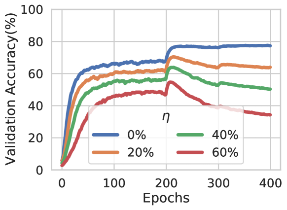
(a) Validation Accuracy

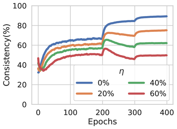
(b) Consistency

Figure 1: Evolution of a trained network’s consistency as it overfits to noise using CE loss. Here we plot the evolution of the validation accuracy (a) and network’s consistency (b) on the training set of CIFAR-100 for varying symmetric noise rates when learning with the cross-entropy loss. The consistency of the learnt function and the accuracy closely correlate. Assuming causation, suggests that enforcing consistency may help avoid fitting to noise.

2 Consistency for Learning with Label Noise

In this section, we first make two intriguing observations which motivate the use of consistency regularization for learning with noisy labels. Then we propose a loss function to this end preceded with some necessary background.

2.1 Consistency When Overfitting to Noise

In Figure 1, we show the evolution of (a) the validation accuracy and (b) a measure of consistency during training with the CE loss for varying amounts of noise. First, we note that training with CE loss eventually overfits to the noisy labels. Figure 1(b) shows the consistency of predictions w.r.t. the CIFAR-100 training set. Consistency is measured as the fraction of images that have the same class prediction for the original image and an augmented version of it, see Appendix C for more details. Interestingly, a clear correlation is observed between validation accuracy and training consistency. Assuming causality, suggests that maximizing consistency of predictions may improve robustness to noise.

In Figure 2, similarly to Figure 1, we study the consistency among training examples, but separately for those with noisy/wrong labels and those with clean/correct labels. Crucially, we find that the consistency around noisy examples degrades more significantly than for clean examples. This suggests that encouraging noisy examples to stay consistent will make it harder to overfit to noise.

Based on these observations, we propose a loss function to encourage consistency in Section 2.3. Before presenting the loss function, we briefly reiterate some background.

2.2 Background

Supervised Classification. Given a training dataset $\mathcal{D}=\{({\bm{x}}_{i},y_{i})\}_{i=1}^{N}$, our goal is to learn the parameters of a softmax neural network ($f$) mapping each ${\bm{x}}\in{\mathbb{X}}$ to its corresponding onehot representation (${\bm{y}}$) of the class $y\in{\mathbb{Y}}=\{1,2,\dots,K\}$. The function $f$ is trained on $\mathcal{D}$ by minimizing an empirical risk $\frac{1}{N}\sum_{i=1}^{N}\mathcal{L}({\bm{y}}_{i},f({\bm{x}}_{i}))$, where $\mathcal{L}$ is a loss function.

Learning with Noisy Labels. In this work, we learn from a noisy training distribution $\mathcal{D}_{\eta}$ where the labels are changed, with probability $\eta$, from their true distribution $\mathcal{D}$. The noise is called symmetric if the noisy label is independent of the true label and asymmetric if it is class dependent. The considered noise in this work is sample-independent.

2.3 Consistency Loss

There are many ways to encourage consistency between predictions. Most methods combine a label-dependent term (typically cross-entropy) with a separate label-independent consistency term based on $l^{2}$-norm (Tarvainen & Valpola, 2017), CE (Miyato et al., 2018), etc. Here, similar to AugMix (Hendrycks et al., 2020), we use a loss based on Jensen-Shannon divergence to encourage consistency.

Let ${\bm{y}}$ be the onehot label, and ${\bm{p}}_{1},{\bm{p}}_{2}$ be predictions from two augmentations of the same image, and a weight $\pi$ satisfying $0~{}\leq~{}\pi~{}\leq 1$, then our loss is

$$\mathrm{GJS}\coloneqq\mathrm{JS}_{\pi}({\bm{y}},\frac{{\bm{p}}_{1}+{\bm{p}}_{2}}{2})+(1-\pi)\mathrm{JS}_{\frac{1}{2}}({\bm{p}}_{1},{\bm{p}}_{2})$$ (1)

where $\mathrm{JS}_{\pi}$ is the Jensen-Shannon divergence

$$\mathrm{JS}_{\pi}({\bm{p}}_{1},{\bm{p}}_{2})\coloneqq\pi\mathrm{KL}({\bm{p}}_{1}\|{\bm{m}})+(1-\pi)\mathrm{KL}({\bm{p}}_{2}\|{\bm{m}})$$ (2)

with the mean ${\bm{m}}\coloneqq\pi{\bm{p}}_{1}+(1-\pi){\bm{p}}_{2}$.

The two $\mathrm{JS}_{\pi}$ terms of $\mathrm{GJS}$ in Equation 1 encourage the predictions to be close to the label and to be consistent, respectively. For the label-dependent term, we treat $\pi$ as a hyperparameter, while the consistency term uses equal weights ($\pi=\frac{1}{2}$). We also use the loss $\mathrm{JS}\coloneqq\mathrm{JS}_{\pi}({\bm{y}},{\bm{p}}_{1})$ as a baseline to compare with a Jensen-Shannon-based loss without consistency. Indeed, $\mathrm{GJS}$ generalizes $\mathrm{JS}$ by incorporating consistency regularization.

The main design choices here are what divergences to use for the label-dependent term and the consistency term. Indeed, a difference between our loss and AugMix is the use of $\mathrm{JS}$ for both terms. This is not an arbitrary choice, but has theoretical justifications when learning with noisy labels (Englesson & Azizpour, 2021).

3 Experiments

This section, empirically investigates the effectiveness of the proposed losses for learning with noisy labels, on synthetic (Section 3.1) and real-world noise (Section 3.2). In Section 3.3, we perform an ablation study to substantiate the importance of the consistency term, when going from $\mathrm{JS}$ to $\mathrm{GJS}$. All these additional experiments are done on the more challenging CIFAR-100 dataset.

Experimental Setup. We use ResNet 34 and 50 for experiments on CIFAR and WebVision datasets respectively and optimize them using SGD with momentum. The complete details of the training setup can be found in Appendix A. Most importantly, we take three main measures to ensure a fair and reliable comparison throughout the experiments: 1) we reimplement all the loss functions we compare with in a single shared learning setup, 2) we use the same hyperparameter optimization budget and mechanism for all the prior works and ours, and 3) we train and evaluate five networks for individual results, where in each run the synthetic noise, network initialization, and data-order are differently randomized. The thorough analysis is evident from the higher performance of CE in our setup compared to prior works. Where possible, we report mean and standard deviation and denote the statistically-significant top performers with student t-test.

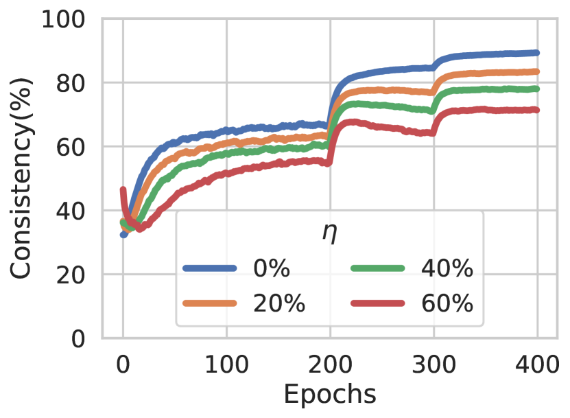
(a) Consistency Clean

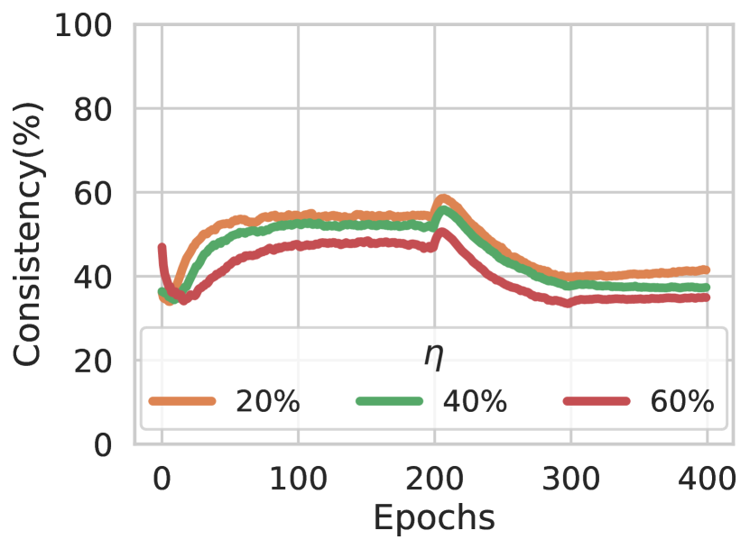
(b) Consistency Noisy

Figure 2: Consistency of clean and noisy examples. Consistency of correct (clean) and mislabelled (noisy) examples when overfitting to noise for various noise rates on CIFAR-100. The consistency is significantly degraded for the noisy data points.

3.1 Synthetic Noise Benchmarks: CIFAR

Here, we evaluate the proposed loss functions on the CIFAR datasets with two types of synthetic noise: symmetric and asymmetric, see Appendix A.1 for details.

We compare with other noise-robust loss functions such as Bootstrap (BS) (Reed et al., 2014), Symmetric Cross-Entropy (SCE) (Wang et al., 2019), and Generalized Cross-Entropy (GCE) (Zhang & Sabuncu, 2018), We do not compare to methods that propose a full pipeline since, first, a conclusive comparison would require re-implementation and individual evaluation of several components and second, robust loss functions can be complementary to them.

Results. Table 1 shows the results for symmetric and asymmetric noise on CIFAR-10 and CIFAR-100. $\mathrm{GJS}$ performs similarly or better than other methods for different noise rates, noise types, and data sets. Generally, $\mathrm{GJS}$’s efficacy is more evident for the more challenging CIFAR-100 dataset. For example, on 60% uniform noise on CIFAR-100, the difference between $\mathrm{GJS}$ and the second best (GCE) is 4.94 percentage points. Interestingly, the performance of $\mathrm{JS}$ is consistently similar to the top performance of the prior works across different noise rates, types and datasets. Next, we test $\mathrm{GJS}$ on a naturally-noisy dataset to see its efficacy in a real-world scenario.

Table 1: Synthetic Noise Benchmark on CIFAR. We reimplement other noise-robust loss functions into the same learning setup and ResNet-34, including Bootstrap (BS), Generalized CE (GCE), and Symmetric Cross Entropy (SCE). We used same hyperparameter optimization budget and mechanism for all the prior works and ours. Mean test accuracy and standard deviation are reported from five runs and the statistically-significant top performers are boldfaced. $\mathrm{GJS}$ achieves state-of-the-art results for different noise rates, types, and datasets. Generally, $\mathrm{GJS}$’s efficacy is more evident for the more challenging CIFAR-100 dataset.

Dataset	Loss	No Noise	Symmetric Noise Rate		Asymmetric Noise Rate
		0%	20%	60%	20%	40%
C10	CE	95.77 $\pm$ 0.11	91.63 $\pm$ 0.27	81.99 $\pm$ 0.56	92.77 $\pm$ 0.24	87.12 $\pm$ 1.21
	BS	94.58 $\pm$ 0.25	91.68 $\pm$ 0.32	82.65 $\pm$ 0.57	93.06 $\pm$ 0.25	88.87 $\pm$ 1.06
	SCE	95.75 $\pm$ 0.16	94.29 $\pm$ 0.14	89.26 $\pm$ 0.37	93.48 $\pm$ 0.31	84.98 $\pm$ 0.76
	GCE	95.75 $\pm$ 0.14	94.24 $\pm$ 0.18	89.37 $\pm$ 0.27	92.83 $\pm$ 0.36	87.00 $\pm$ 0.99
	JS	95.89 $\pm$ 0.10	94.52 $\pm$ 0.21	89.64 $\pm$ 0.15	92.18 $\pm$ 0.31	87.99 $\pm$ 0.55
	GJS	95.91 $\pm$ 0.09	95.33 $\pm$ 0.18	91.64 $\pm$ 0.22	93.94 $\pm$ 0.25	89.65 $\pm$ 0.37
C100	CE	77.60 $\pm$ 0.17	65.74 $\pm$ 0.22	44.42 $\pm$ 0.84	66.85 $\pm$ 0.32	49.45 $\pm$ 0.37
	BS	77.65 $\pm$ 0.29	72.92 $\pm$ 0.50	53.80 $\pm$ 1.76	73.79 $\pm$ 0.43	64.67 $\pm$ 0.69
	SCE	78.29 $\pm$ 0.24	74.21 $\pm$ 0.37	59.28 $\pm$ 0.58	70.86 $\pm$ 0.44	51.12 $\pm$ 0.37
	GCE	77.65 $\pm$ 0.17	75.02 $\pm$ 0.24	65.21 $\pm$ 0.16	72.13 $\pm$ 0.39	51.50 $\pm$ 0.71
	JS	77.95 $\pm$ 0.39	75.41 $\pm$ 0.28	64.36 $\pm$ 0.34	71.70 $\pm$ 0.36	49.36 $\pm$ 0.25
	GJS	79.27 $\pm$ 0.29	78.05 $\pm$ 0.25	70.15 $\pm$ 0.30	74.60 $\pm$ 0.47	63.70 $\pm$ 0.22

3.2 Real-World Noise Benchmark: WebVision

WebVision v1 is a large-scale image dataset collected by crawling Flickr and Google, which resulted in an estimated 20% of noisy labels (Li et al., 2017). There are 2.4 million images of the same thousand classes as ILSVRC12. Here, we use a smaller version called mini WebVision (Jiang et al., 2018) consisting of the first 50 classes of the Google subset.

Results. Table 2, as the common practice, reports the performances on the validation sets of WebVision and ILSVRC12 (first 50 classes). Both $\mathrm{JS}$ and $\mathrm{GJS}$ exhibits large margins with standard CE, especially using top-1 accuracy. Top-5 accuracy, due to its admissibility of wrong top predictions, can obscure the susceptibility to noise-fitting and thus indicates smaller but still significant improvements.

The two state-of-the-art methods on this dataset were DivideMix(Li et al., 2020a) and ELR+(Liu et al., 2020). Compared to our setup, both these methods use a stronger network (Inception-ResNet-V2 vs ResNet-50), stronger augmentations (Mixup vs color jittering) and co-train two networks instead of a single one. Furthermore, ELR+ uses an exponential moving average of weights and DivideMix treats clean and noisy labelled examples differently after separating them using Gaussian mixture models. Despite these differences, $\mathrm{GJS}$ performs as good or better in terms of top-1 accuracy on WebVision and significantly outperforms ELR+ on ILSVRC12 (70.29 vs 74.33).

So far, the experiments demonstrated the robustness of the proposed loss function via the significant improvements of final accuracy on noisy datasets. While this was central and informative, it is also important to investigate whether this improvement come from the properties that were argued for $\mathrm{GJS}$. In what follows, we devise such experiments.

Table 2: Real-world Noise Benchmark on WebVision. Mean test accuracy and standard deviation from five runs are reported for the validation sets of (mini) WebVision and ILSVRC12. Results marked with $\dagger$ are from (Zheltonozhskii et al., 2021). DivideMix with $\star$ uses a ResNet-50 (used by CE, $\mathrm{JS}$, $\mathrm{GJS}$) instead of InceptionResNet-V2.

Method	WebVision		ILSVRC12
	Top 1	Top 5	Top 1	Top 5
ELR+$\dagger$	$\bm{77.78}$	$\bm{91.68}$	70.29	89.76
DivideMix$\dagger$	77.32	$\bm{91.64}$	$\bm{75.20}$	90.84
DivideMix$\star\dagger$	76.32 $\pm$ 0.36	90.65 $\pm$ 0.16	74.42 $\pm$ 0.29	$\bm{91.21\pm 0.12}$
CE	70.69 $\pm$ 0.66	88.64 $\pm$ 0.17	67.32 $\pm$ 0.57	88.00 $\pm$ 0.49
JS	74.56 $\pm$ 0.32	91.09 $\pm$ 0.08	70.36 $\pm$ 0.12	90.60 $\pm$ 0.09
GJS	$\bm{77.99\pm 0.35}$	90.62 $\pm$ 0.28	74.33 $\pm$ 0.46	90.33 $\pm$ 0.20

3.3 Towards a Better Understanding of GJS

Is the improvements of GJS over JS due to mean prediction or consistency? The difference between $\mathrm{JS}$ and $\mathrm{GJS}$ is the mean prediction in the label-dependent term and the consistency term. In Table 3, we study these differences by using $\mathrm{GJS}$ without the consistency term, i.e., $\mathrm{JS}({\bm{y}},{\bm{m}})$. The results suggest that the improvement of $\mathrm{GJS}$ over $\mathrm{JS}$ can be crucially attributed to the consistency term.

Is GJS mostly helping the clean or noisy examples? To better understand the improvements of $\mathrm{GJS}$ over $\mathrm{JS}$, we perform an ablation with different losses for clean and noisy examples, see Table 4. Using $\mathrm{GJS}$ instead of $\mathrm{JS}$ improves performance in all cases. Importantly, using $\mathrm{GJS}$ only for the noisy examples performs significantly better than only using it for the clean examples (74.1 vs 72.9). The best result is achieved when using $\mathrm{GJS}$ for both clean and noisy examples but still close to the noisy-only case (74.7 vs 74.1).

Additional Experiments. In Appendix D, we study the role of augmentations and the training behavior of $\mathrm{GJS}$.

Table 3: Effect of Consistency. Validation accuracy for $\mathrm{JS}$, $\mathrm{GJS}$ w/o the consistency term in Equation 1, and $\mathrm{GJS}$ for $40\%$ noise on the CIFAR-100 dataset. Using the mean of two predictions in the $\mathrm{JS}$ loss does not improve performance. On the other hand, adding the consistency term significantly helps.

Method	Accuracy
$\mathrm{JS}_{\pi}({\bm{y}},{\bm{p}}_{1})$	71.0
$\mathrm{JS}_{\pi}({\bm{y}},{\bm{m}})$	68.7
$\mathrm{GJS}$	74.3

Table 4: Effect of $\bm{\mathrm{GJS}}$. Validation accuracy when using different loss functions for clean and noisy examples of the CIFAR-100 training set with 40% symmetric noise. Noisy examples benefit significantly more from $\mathrm{GJS}$ than clean examples (74.1 vs 72.9).

Method		$\pi$
Clean	Noisy	0.1	0.5	0.9
JS	JS	70.0	$\bm{71.5}$	55.3
GJS	JS	72.6	$\bm{72.9}$	70.2
JS	GJS	71.0	$\bm{74.1}$	68.0
GJS	GJS	71.3	$\bm{74.7}$	73.8

4 Related Works

Consistency regularization is a recent technique that imposes smoothness in the learnt function for semi-supervised learning (Oliver et al., 2018) and recently for noisy data (Li et al., 2020a). These works use complex pipelines for such regularization. $\mathrm{GJS}$ encourages consistency in a simple way that exhibits other desirable properties for learning with noisy labels. Importantly, Hendrycks et al. (2020) used Jensen-Shannon-based loss functions to improve test-time robustness to image corruptions which further verifies the general usefulness of $\mathrm{GJS}$. In this work, we study such loss functions for the different goal of training-time label-noise robustness. In this context, our thorough analytical and empirical results are, to the best of our knowledge, novel.

Recently, loss functions with information-theoretic motivations have been proposed (Xu et al., 2019; Wei & Liu, 2021). $\mathrm{JS}$, with apparent information-theoretic interpretation, has a strong connection to those. The latter is a close concurrent work but takes a different and complementary angle. The connection of these works can be a fruitful future direction.

5 Final Remarks

Overall, we believe the paper provides useful and novel observations and informative empirical evidence for the usefulness of a JS divergence-based consistency loss for learning under noisy data that achieve state-of-the-art results. At the same time it opens interesting future directions.

Acknowledgement.

This work was partially supported by the Wallenberg AI, Autonomous Systems and Software Program (WASP) funded by the Knut and Alice Wallenberg Foundation.

Appendix A Training Details

Our method and the baselines use the same training settings, which are described in detail here.

A.1 CIFAR

General Training Details. For all the results on the CIFAR datasets, we use a PreActResNet-34 with a standard SGD optimizer with Nesterov momentum, and a batch size of 128. For the network, we use three stacks of five residual blocks with 32, 64, and 128 filters for the layers in these stacks, respectively. The learning rate is reduced by a factor of 10 at 50% and 75% of the total 400 epochs. For data augmentation, we use RandAugment (Cubuk et al., 2019) with $N=1$ and $M=3$ using random cropping (size 32 with 4 pixels as padding), random horizontal flipping, normalization and lastly Cutout (DeVries & Taylor, 2017) with length 16. We set random seeds for all methods to have the same network weight initialization, order of data for the data loader, train-validation split, and noisy labels in the training set. We use a clean validation set corresponding to 10% of the training data. A clean validation set is commonly provided with real-world noisy datasets (Li et al., 2017, 2019). Any potential gain from using a clean instead of a noisy validation set is the same for all methods since all share the same setup.

Noise Types. For symmetric noise, the labels are, with probability $\eta$, re-sampled from a uniform distribution over all labels. For asymmetric noise, we follow the standard setup of Patrini et al. (2017). For CIFAR-10, the labels are modified, with probability $\eta$, as follows: truck $\to$ automobile, bird $\to$ airplane, cat $\leftrightarrow$ dog, and deer $\to$ horse. For CIFAR-100, labels are, with probability $\eta$, cycled to the next sub-class of the same “super-class”, e.g. the labels of super-class “vehicles 1” are modified as follows: bicycle $\rightarrow$ bus $\rightarrow$ motorcycle $\rightarrow$ pickup truck $\rightarrow$ train $\rightarrow$ bicycle.

Search for learning rate and weight decay. We do a separate hyperparameter search for learning rate and weight decay on 40% noise using both asymmetric and symmetric noises on CIFAR datasets. For CIFAR-10, we search for learning rates in $[0.001,0.005,0.01,0.05,0.1]$ and weight decays in $[1e-4,5e-4,1e-3]$. The method-specific hyperparameters used for this search were 0.9, 0.7, (0.1,1.0), 0.7, (1.0,1.0), 0.5, 0.5 for BS($\beta$), LS($\epsilon$), SCE($\alpha,\beta$), GCE($q$), NCE+RCE($\alpha,\beta$), JS($\pi$) and GJS($\pi$), respectively. For CIFAR-100, we search for learning rates in $[0.01,0.05,0.1,0.2,0.4]$ and weight decays in $[1e-5,5e-5,1e-4]$. The method-specific hyperparameters used for this search were 0.9, 0.7, (6.0,0.1), 0.7, (10.0,0.1), 0.5, 0.5 for BS($\beta$), LS($\epsilon$), SCE($\alpha,\beta$), GCE($q$), NCE+RCE($\alpha,\beta$), JS($\pi$) and GJS($\pi$), respectively. Note that, these fixed method-specific hyperparameters for both CIFAR-10 and CIFAR-100 are taken from their corresponding papers for this initial search of learning rate and weight decay but they will be further optimized systematically in the next steps.

Search for method-specific parameters. We fix the obtained best learning rate and weight decay for all other noise rates, but then for each noise rate/type, we search for method-specific parameters. For the methods with a single hyperparameter, BS ($\beta$), LS ($\epsilon$), GCE ($q$), JS ($\pi$), GJS ($\pi$), we try values in $[0.1,0.3,0.5,0.7,0.9]$. On the other hand, NCE+RCE and SCE have three hyperparameters, i.e. $\alpha$ and $\beta$ that scale the two loss terms, and $A\coloneqq\log(0)$ for the RCE term. We set $A=\log{(1e-4)}$ and do a grid search for three values of $\alpha$ and two of beta $\beta$ (six in total) around the best reported parameters from each paper.

Test evaluation. The best parameters are then used to train on the full training set with five different seeds. The final parameters that were used to get the results in Table 1 are shown in Table 5.

Table 5: Hyperparameters for CIFAR. A hyperparameter search over learning rates and weight decays, was done for 40% noise on both symmetric and asymmetric noise for the CIFAR datasets. The best parameters for each method are shown in this table, where the format is [learning rate, weight decay]. The hyperparameters for zero percent noise uses the same settings as for the symmetric noise. For the best learning rate and weight decay, another search is done for method-specific hyperparameters, and the best values are shown here. For methods with a single hyperparameter, the value correspond to their respective hyperparameter, i.e., BS ($\beta$), GCE ($q$), JS ($\pi$), GJS ($\pi$). For SCE the value correspond to [$\alpha$, $\beta$].

Dataset	Method	Learning Rate & Weight Decay		Method-specific Hyperparameters
		Sym Noise	Asym Noise	No Noise	Sym Noise		Asym Noise
		20-60%	20-40%	0%	20%	60%	20%	40%
CIFAR-10	CE	[0.05, 1e-3]	[0.1, 1e-3]	-	-	-	-	-
	BS	[0.1, 1e-3]	[0.1, 1e-3]	0.5	0.5	0.7	0.7	0.5
	SCE	[0.01, 5e-4]	[0.05, 1e-3]	[0.2, 0.1]	[0.05, 0.1]	[0.2, 1.0]	[0.1, 0.1]	[0.2, 1.0]
	GCE	[0.01, 5e-4]	[0.1, 1e-3]	0.5	0.7	0.7	0.1	0.1
	JS	[0.01, 5e-4]	[0.1, 1e-3]	0.1	0.7	0.9	0.3	0.3
	GJS	[0.1, 5e-4]	[0.1, 1e-3]	0.5	0.3	0.1	0.3	0.3
CIFAR-100	CE	[0.4, 1e-4]	[0.2, 1e-4]	-	-	-	-	-
	BS	[0.4, 1e-4]	[0.4, 1e-4]	0.7	0.5	0.5	0.3	0.3
	SCE	[0.2, 1e-4]	[0.4, 5e-5]	[0.1, 0.1]	[0.1, 0.1]	[0.1, 1.0]	[0.1, 1.0]	[0.1, 1.0]
	GCE	[0.4, 1e-5]	[0.2, 1e-4]	0.5	0.5	0.7	0.7	0.7
	JS	[0.2, 1e-4]	[0.1, 1e-4]	0.1	0.1	0.5	0.5	0.5
	GJS	[0.2, 5e-5]	[0.4, 1e-4]	0.3	0.3	0.9	0.5	0.1

A.2 WebVision

All methods train a randomly initialized ResNet-50 model from PyTorch using the SGD optimizer with Nesterov momentum, and a batch size of 32 for $\mathrm{GJS}$ and 64 for CE and $\mathrm{JS}$. For data augmentation, we do a random resize crop of size 224, random horizontal flips, and color jitter (torchvision ColorJitter transform with brightness=0.4, contrast=0.4, saturation=0.4, hue=0.2). We use a fixed weight decay of $1e-4$ and do a grid search for the best learning rate in $[0.1,0.2,0.4]$ and $\pi\in[0.1,0.3,0.5,0.7,0.9]$. The learning rate is reduced by a multiplicative factor of $0.97$ every epoch, and we train for a total of 300 epochs. The best starting learning rates were 0.4, 0.2, 0.1 for CE, JS and GJS, respectively. Both $\mathrm{JS}$ and $\mathrm{GJS}$ used $\pi=0.1$. With the best learning rate and $\pi$, we ran four more runs with new seeds for the network initialization and data loader.

Appendix B Loss Implementation Details

Loss. We implement the Jensen-Shannon divergence using the definitions based on KL divergence, see Equation 2. To make sure the gradients are propagated through the target argument, we do not use the built-in KL divergence in PyTorch. Instead, we write our own based on the official implementation.

Scaling. The value of the $\mathrm{JS}_{\pi}$ divergence becomes small as the hyperparameter $\pi$ approaches 0 and 1. To counteract this, we divide both $\mathrm{JS}$ and $\mathrm{GJS}$ losses by a constant factor, $-(1-\pi)\log(1-\pi)$. Clearly, this scaling is equivalent to a scaling of the learning rate.

Appendix C Consistency Measure

In this section, we provide more details about the consistency measure used in e.g. Figure 1. To be independent of any particular loss function, we considered a measure similar to standard Top-1 accuracy. We measure the ratio of samples that predict the same class on both the original image and an augmented version of it

$$\frac{1}{N}\sum_{i=1}^{N}\mathbbm{1}\big{(}\operatorname*{arg\,max}_{y}f({\bm{x}}_{i})=\operatorname*{arg\,max}_{y}f(\tilde{{\bm{x}}}_{i})\big{)}$$ (3)

where the sum is over all the training examples, and $\mathbbm{1}$ is the indicator function, the argmax is over the predicted probability of $K$ classes, and $\tilde{{\bm{x}}}_{i}$ is an augmented version of ${\bm{x}}_{i}$. Notably, this measure does not depend on the labels.

In the experiments in Figure 1 and 2, the original images are only normalized, while the augmented images use the same augmentation strategy as the benchmark experiments in Section A.1.

Appendix D Additional Experiments

D.1 Augmentations

As described in Section A.1, our augmentation strategy is composed of several transformations: random crop, horizontal flips, CutOut, and RandAugment. Here, we study the noise-robustness of our method when removing some of these transformations. We either remove CutOut, RandAugment, or both (which we denote by “weak”). See Table 6 for the results of 40% symmetric and asymmetric noise rates on CIFAR-100. While more transformations help improve robustness for all methods, it is not required for $\mathrm{GJS}$ to perform well.

Table 6: Effect of Augmentation Strategy. Validation accuracy for training w/o CutOut(-CO) or w/o RandAug(-RA) or w/o both(weak) on 40% symmetric and asymmetric noise on CIFAR-100. All methods improves by stronger augmentations. GJS performs best for all types of augmentations.

Method	Symmetric				Asymmetric
	Full	-CO	-RA	Weak	Full	-CO	-RA	Weak
GCE	70.8	64.2	64.1	58.0	51.7	44.9	46.6	42.9
NCE+RCE	68.5	66.6	68.3	61.7	57.5	52.1	49.5	44.4
GJS	$\bm{74.8}$	$\bm{71.3}$	$\bm{70.6}$	$\bm{66.5}$	62.6	56.8	52.2	44.9

D.2 Training Behavior of Networks using GJS

In Section 2.1, we observed that networks become less consistent when trained with the CE loss on noisy data, especially the consistency of predictions on the noisy labelled examples. To better understand the improvements in robustness that $\mathrm{GJS}$ brings to the learning dynamics of deep networks, we compare CE and $\mathrm{GJS}$ in Figure 3 in terms of training accuracy and consistency for clean and noisy labelled examples. For clean (correctly) labelled examples, $\mathrm{GJS}$ improves the accuracy and consistency to be as good as without any noise. For noisy (mislabelled) examples, we observe that $\mathrm{GJS}$ significantly reduces the overfitting to noisy labels and keeps improving the consistency.

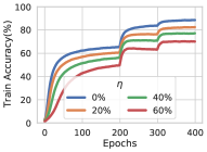
(a) CE - Clean

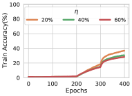
(b) CE - Noisy

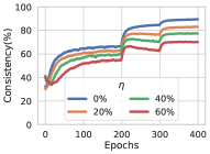
(c) CE - Clean

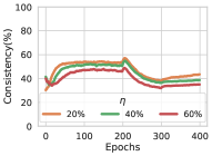
(d) CE - Noisy

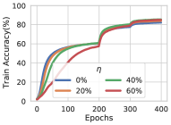
(e) GJS - Clean

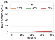
(f) GJS - Noisy

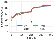
(g) GJS - Clean

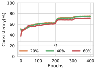
(h) GJS - Noisy

Figure 3: Evolution of training accuracy and consistency for clean and noisy examples. Consistency and training accuracy of correct (clean) and mislabelled (noisy) examples when overfitting to noise for various symmetric noise rates on CIFAR-100 for the CE and $\mathrm{GJS}$ losses. $\mathrm{GJS}$ uses $\pi=0.9$, and both CE and GJS use the same learning rate ($0.2$) and weight decay ($5e-5$) for all noise rates. Using $\mathrm{GJS}$ as a loss keeps the network’s predictions consistent (e.g. (d) and (h)) and significantly reduces the overfitting to noise ((b) and (f)). Interestingly, $\mathrm{GJS}$ also significantly improves the clean training accuracy when learning with noisy labels ((a) and (e)).

References

- Berthelot et al. (2019) Berthelot, D., Carlini, N., Goodfellow, I., Papernot, N., Oliver, A., and Raffel, C. A. Mixmatch: A holistic approach to semi-supervised learning. In Advances in Neural Information Processing Systems, pp. 5049–5059, 2019.
- Beyer et al. (2020) Beyer, L., Hénaff, O. J., Kolesnikov, A., Zhai, X., and Oord, A. v. d. Are we done with imagenet? arXiv preprint arXiv:2006.07159, 2020.
- Cubuk et al. (2019) Cubuk, E. D., Zoph, B., Shlens, J., and Le, Q. V. Randaugment: Practical automated data augmentation with a reduced search space, 2019.
- DeVries & Taylor (2017) DeVries, T. and Taylor, G. W. Improved regularization of convolutional neural networks with cutout, 2017.
- Englesson & Azizpour (2021) Englesson, E. and Azizpour, H. Generalized jensen-shannon divergence loss for learning with noisy labels, 2021.
- Ghosh et al. (2017) Ghosh, A., Kumar, H., and Sastry, P. Robust loss functions under label noise for deep neural networks. In Proceedings of the Thirty-First AAAI Conference on Artificial Intelligence, pp. 1919–1925, 2017.
- Hendrycks et al. (2020) Hendrycks, D., Mu, N., Cubuk, E. D., Zoph, B., Gilmer, J., and Lakshminarayanan, B. Augmix: A simple data processing method to improve robustness and uncertainty. In International Conference on Learning Representation, 2020.
- Iscen et al. (2020) Iscen, A., Tolias, G., Avrithis, Y., Chum, O., and Schmid, C. Graph convolutional networks for learning with few clean and many noisy labels. In Proceedings of the European Conference on Computer Vision, 2020.
- Jiang et al. (2018) Jiang, L., Zhou, Z., Leung, T., Li, J., and Li, F.-F. Mentornet: Learning data-driven curriculum for very deep neural networks on corrupted labels. In ICML, 2018.
- Li et al. (2019) Li, J., Wong, Y., Zhao, Q., and Kankanhalli, M. Learning to learn from noisy labeled data, 2019.
- Li et al. (2020a) Li, J., Socher, R., and Hoi, S. C. Dividemix: Learning with noisy labels as semi-supervised learning. In International Conference on Learning Representation, 2020a.
- Li et al. (2020b) Li, M., Soltanolkotabi, M., and Oymak, S. Gradient descent with early stopping is provably robust to label noise for overparameterized neural networks. In International Conference on Artificial Intelligence and Statistics, pp. 4313–4324. PMLR, 2020b.
- Li et al. (2017) Li, W., Wang, L., Li, W., Agustsson, E., and Gool, L. V. Webvision database: Visual learning and understanding from web data, 2017.
- Liu et al. (2020) Liu, S., Niles-Weed, J., Razavian, N., and Fernandez-Granda, C. Early-learning regularization prevents memorization of noisy labels, 2020.
- Liu & Guo (2020) Liu, Y. and Guo, H. Peer loss functions: Learning from noisy labels without knowing noise rates. In III, H. D. and Singh, A. (eds.), Proceedings of the 37th International Conference on Machine Learning, volume 119 of Proceedings of Machine Learning Research, pp. 6226–6236. PMLR, 13–18 Jul 2020.
- Lukasik et al. (2020) Lukasik, M., Bhojanapalli, S., Menon, A. K., and Kumar, S. Does label smoothing mitigate label noise? In International Conference on Machine Learning, 2020.
- Ma et al. (2020) Ma, X., Huang, H., Wang, Y., Romano, S., Erfani, S., and Bailey, J. Normalized loss functions for deep learning with noisy labels, 2020.
- Miyato et al. (2018) Miyato, T., Maeda, S.-i., Koyama, M., and Ishii, S. Virtual adversarial training: a regularization method for supervised and semi-supervised learning. IEEE transactions on pattern analysis and machine intelligence, 41(8):1979–1993, 2018.
- Nguyen et al. (2019) Nguyen, D. T., Mummadi, C. K., Ngo, T. P. N., Nguyen, T. H. P., Beggel, L., and Brox, T. Self: Learning to filter noisy labels with self-ensembling. In International Conference on Learning Representation, 2019.
- Northcutt et al. (2017) Northcutt, C. G., Wu, T., and Chuang, I. L. Learning with confident examples: Rank pruning for robust classification with noisy labels. arXiv preprint arXiv:1705.01936, 2017.
- Oliver et al. (2018) Oliver, A., Odena, A., Raffel, C., Cubuk, E. D., and Goodfellow, I. J. Realistic evaluation of deep semi-supervised learning algorithms. arXiv preprint arXiv:1804.09170, 2018.
- Patrini et al. (2017) Patrini, G., Rozza, A., Menon, A., Nock, R., and Qu, L. Making deep neural networks robust to label noise: a loss correction approach, 2017.
- Reed et al. (2014) Reed, S., Lee, H., Anguelov, D., Szegedy, C., Erhan, D., and Rabinovich, A. Training deep neural networks on noisy labels with bootstrapping. arXiv preprint arXiv:1412.6596, 2014.
- Seo et al. (2019) Seo, P. H., Kim, G., and Han, B. Combinatorial inference against label noise. In Advances in Neural Information Processing Systems, pp. 1173–1183, 2019.
- Tanaka et al. (2018) Tanaka, D., Ikami, D., Yamasaki, T., and Aizawa, K. Joint optimization framework for learning with noisy labels. In Proceedings of the IEEE Conference on Computer Vision and Pattern Recognition, pp. 5552–5560, 2018.
- Tarvainen & Valpola (2017) Tarvainen, A. and Valpola, H. Mean teachers are better role models: Weight-averaged consistency targets improve semi-supervised deep learning results. In Advances in neural information processing systems, pp. 1195–1204, 2017.
- Vahdat (2017) Vahdat, A. Toward robustness against label noise in training deep discriminative neural networks. In Advances in Neural Information Processing Systems, pp. 5596–5605, 2017.
- Wang et al. (2019) Wang, Y., Ma, X., Chen, Z., Luo, Y., Yi, J., and Bailey, J. Symmetric cross entropy for robust learning with noisy labels. In Proceedings of the IEEE International Conference on Computer Vision, pp. 322–330, 2019.
- Wei & Liu (2021) Wei, J. and Liu, Y. When optimizing f-divergence is robust with label noise. In International Conference on Learning Representation, 2021.
- Xu et al. (2019) Xu, Y., Cao, P., Kong, Y., and Wang, Y. L_dmi: A novel information-theoretic loss function for training deep nets robust to label noise. In Advances in Neural Information Processing Systems, pp. 6225–6236, 2019.
- Zhang & Sabuncu (2018) Zhang, Z. and Sabuncu, M. Generalized cross entropy loss for training deep neural networks with noisy labels. In Advances in neural information processing systems, pp. 8778–8788, 2018.
- Zheltonozhskii et al. (2021) Zheltonozhskii, E., Baskin, C., Mendelson, A., Bronstein, A. M., and Litany, O. Contrast to divide: Self-supervised pre-training for learning with noisy labels, 2021.