Revisiting the cosmic distance duality relation with machine learning reconstruction methods: the combination of HII galaxies and ultra-compact radio quasars

Abstract

In this paper, we carry out an assessment of cosmic distance duality relation (CDDR) based on the latest observations of HII galaxies acting as standard candles and ultra-compact structure in radio quasars acting as standard rulers. Particularly, two machine learning reconstruction methods (Gaussian Process (GP) and Artificial Neural Network (ANN)) are applied to reconstruct the Hubble diagrams from observational data. We show that both approaches are capable of reconstructing the current constraints on possible deviations from the CDDR in the redshift range $z\sim 2.3$. Considering four different parametric methods of CDDR, which quantify deviations from the CDDR and the standard cosmological model, we compare the results of the two different machine learning approaches. It is observed that the validity of CDDR is in well agreement with the current observational data within $1\sigma$ based on the reconstructed distances through GP in the overlapping redshift domain. Moreover, we find that ultra-compact radio quasars could provide $10^{-3}$-level constraints on the violation parameter at high redshifts, when combined with the observations of HII galaxies. In the framework of ANN, one could derive robust constraints on the violation parameter at a precision of $10^{-2}$, with the validity of such distance duality relation within $2\sigma$ confidence level.

1 Introduction

The cosmic distance duality relation (CDDR) is a fundamental relation in modern cosmology, which relates two cosmologiccal distances in cosmology (i.e. the luminosity distance $D_{L}(z)$ and angular diameter distance $D_{A}(z)$). More specifically, the CDDR indicates that $D_{L}(z)$ and $D_{A}(z)$ satisfy the relation of $D_{L}(z)=D_{A}(z)(1+z)^{2}$ at the same redshift 1 ; 2 . Theoretically, the validity of the CDDR depends on three basic assumptions: i)the space-time is described by a metric theory; ii)the light travels along the null geodesics between the source and the observer; iii)the photon number is conserved. Moreover, one of the basic assumptions of general relativity is that photons travel along null geodesics. In other word, the validity of the CDDR can be a support of general relativity in some extents. As a fundamental relation, the CDDR has been widely used in varieties of research fields in astronomy, such as the large-scale distribution of galaxies and the near-uniformity of the CMB temperature 3 , as well as the gas mass density profile and temperature profile of galaxy clusters Cao11a ; Cao16 . Various astrophysical mechanisms, such as gravitational lensing, and dust extinction, may cause the deviation of the CDDR from the view of observation. More specifically, photons emitted from the source are affected in the process of propagation due to gravitational lensing effects and dust extinctions. Consequently, the necessary conditions for maintaining the CDDR are violated. Therefore, it is necessary to test the reliability of the CDDR accurately before applying to various astronomical theories.

Traditionally, testing CDDR needs two types of observational data sets, i.e., the luminosity distance derived from the luminous sources with known (or standardizable) intrinsic luminosity in the Universe like type-Ia supernova (SN Ia), and the angular diameter distance observed from Baryon Acoustic Oscillations (BAO) 4 , Sunyaev-Zeldovich (SZ) effect in clusters with X-ray surface luminosity measurements 5 ; Cao11b ; 6 , or strong gravitational lensing (SGL) 7 ; 8 , etc. However, it is necessary to point out that the luminosity distance inferred from SN Ia only covers the relatively lower redshift range $z\leq 1.4$. The so-called ”nuisance” parameter of SN Ia usually optimizes along with model parameters in the chosen cosmological model 9 . Meanwhile, the angular diameter distance derived from BAO or SZ effect is strongly model-dependent, thus will bring systematic uncertainties which are hard to quantify and affect the validity of testing CDDR. In addition, other works 10 ; 11 ; 12 attempted to apply the BAO observations to CDDR test, which also suffers from the limited sample size and low redshift range $0.35\leq z\leq 0.74$. Therefore, in order to perform the validity of testing CDDR, one needs to reduce the statistical uncertainty by increasing the depth and quality of the observed data set. Meanwhile, the redshift ranges of the two samples that inferred the angular diameter distance and the luminosity distance should be roughly consistent. Such issue has been recently discussed in Ref. Zheng21 , focusing on a new idea of testing CDDR through the multiple measurements of high-redshift quasars.

Although many efforts have been made to perform robust tests of CDDR, the lack of adequate observational samples and model-independent methods should be taken into account. Specially, it is difficult to obtain samples that satisfy both the luminosity distance and the angular diameter distance in roughly the same redshift range. This redshift-matching problem problem was recognized a long time ago Cao11b , with a heuristic suggestion that the choice of redshfit difference $\Delta z$ could play an important role in model-independent tests of such relation. More recently, many authors presented a new way to constrain the CDDR with different machine learning algorithms 12a ; 12b ; 12d , with the luminosity distance and angular diameter distance reconstructed from complementary external probes (Type Ia supernovae and gravitational wave (GW) standard sirens) 12c . Their results demonstrated the effectiveness of machine learning approaches in the high-precision test of the electromagnetic and gravitational distance duality relations. More importantly, considering the fact that the purpose of modern cosmology is to establish consistent and robust theories, all alternative methods of testing the fundamental principles of cosmology are necessary. In this paper, we will use two non-parameterized methods, Gaussian Process (GP) and Artificial Neural Network (ANN) algorithm, to reconstruct the newest observations of HII galaxy Hubble diagram and ultra-compact structure of radio quasars, respectively. These two approaches are data-driven and have no assumptions about the data, suggesting that they are completely model-independent. The luminosity distance is inferred from reconstructed HII galaxy Hubble diagram and the angular diameter distance is obtained from the angular-size relation of compact radio quasar. The advantage of using these two data is that the redshift ranges of the two samples are roughly consistent, and can reach a relatively high redshift range $z\sim 2.33$. Since no models were assumed in our analysis, our method produced a clear measurement on the CDDR.

This paper is organized as follows: in Section 2 we briefly introduce methodology of deriving two different cosmological distances from the HII galaxies (including extragalactic HII regions) and ultra-compact structure of radio quasar sources, respectively. The two non-parameterized methods, GP and ANN reconstructing the two data sets are described in Section 3. In Section 4, we show the methodology of measuring CDDR and show our results. Finally, we summarize our conclusions in Section 5.

2 Data and Methodology

2.1 Luminosity distances from HII galaxies and extragalactic HII regions

In order to measure luminosity distances in the Universe, we always turn to sources that have known (or standardised) intrinsic luminosity, such as type-Ia supernova (SN Ia) 9 , more distant quasars 13 ; 14 ; 15 ; 16 , and gamma-ray bursts (GRB) 17 , etc. In addition, the HII galaxies and extragalactic HII regions 18 ; 19 ; 20 constitute a large fraction of population that can be observed up to very high redshifts, beyond the feasible limits of supernova studies. It is well known that the luminosity $L($H$\beta)$ in H$\beta$ and the ionized gas velocity dispersion $\sigma$ of HII galaxies and extragalactic HII regions may have a quantitative relation (be known as “$L$–$\sigma$” relation). The physics behind this relation is based only on a simple idea, i.e., as the mass of the starburst component increases, the number of ionized photons and the turbulent velocity of the gas may both increase as well. Melnick et al. first found that the scatter of “$L$–$\sigma$” relation is very small and have the capability to determine the cosmological distance independent of redshift21 . More specifically, based on the measured flux density (or luminosity) and the turbulent velocity of the gas, one can infer the luminosity distance directly. Whereafter, the validity of the “$L$–$\sigma$” relation acting as the standard candle and its possible cosmological applications have been extensively discussed in the literatures 22 ; 23 ; 24 .

The “$L$–$\sigma$” relation between the luminosity $L($H$\beta)$ in H$\beta$ of a source and its ionized gas velocity dispersion can be expressed as 19

$$\log L(\textrm{H}\beta)=\alpha\log\sigma(\textrm{H}\beta)+\kappa,$$ (1)

where $\alpha$ is the slope and $\kappa$ is the intercept. The $L(\textrm{H}\beta)$ is obtained from the reddening corrected flux density $F(\textrm{H}\beta)$ which only bases on a general equation $L(\textrm{H}\beta)=4\pi D^{2}_{L}F(\textrm{H}\beta)$. Thus, the equation above can be written as a relation of the observed flux density

$$\log D_{L,HII}(z)=0.5[\alpha\log\sigma(\textrm{H}\beta)-\log F(\textrm{H}\beta)+\kappa]-25.04.$$ (2)

Analogous to SN Ia applied in cosmology, the $\alpha$ and $\kappa$ parameters should also be optimized with the assumed cosmological model parameters. Fortunately, Wu et al. used the measurements of Hubble parameters from cosmic clocks (model-independent) to calibrate $\alpha$ and $\kappa$, and demonstrated that the calibrated values $\alpha=5.12\pm 0.08$ and $\kappa=33.08\pm 0.13$ are reliable for cosmological applications 24 . In this work, we will adopt these values with their corresponding uncertainties to get the luminosity distance.

The catalog of spectral and astrometric data from HII galaxies and extragalactic HII regions contain more than 100 sources by far, and its statistical properties can be preliminarily considered in cosmology. In this work, we will use the current observations of 156 HII objects compiled by Terlevich et al. 19 which contain 25 high redshift HII galaxies sources, 107 local HII galaxies sources, and 24 extragalactic HII regions sources covering redshift range $0<z<2.33$. This dataset is larger than the source samples used by Plionis et al. 22 and is more complete than the high redshift data used by Melnick et al. 21 . Full information (including name of the source, redshift, flux density, and turbulent velocity with corresponding observational uncertainties) about the sample of 156 HII regions can be found in Table 1 of the work 20 .

2.2 Angular diameter distances measured from compact structure of radio quasars

Quasars, among the most distant objects in the universe, have great potential as distance indicators. From an observational point of view, there are currently two types of quasar data that can be served as cosmological probes, i.e., the non-linear relation between the ultraviolet and X-ray fluxes of the quasar to construct the Hubble diagram 13 ; 14 ; 15 , and the angular size-distance relation of ultra-compact structures object in radio quasars (QSO) as the standard ruler of cosmology from the very-long-baseline interferometry (VLBI) observations 16 . The first type of quasar data provides the luminosity distance, but not the angular diameter distance, directly. Moreover, although the sample collected by 13 contained 1598 suitable quasars and redshift reaches to $z\sim 5.5$, the sample itself exhibits a large intrinsic dispersion. Take these factors into consideration, we will use the radio quasar sample to obtain the angular diameter distance information.

The angular size-distance relation in compact radio quasar for cosmological inference was first proposed by Kellermann et al. 25 , in which he tried to obtain the deceleration parameter with 79 compact radio sources from VLBI at 5 GHz. Whereafter, Gurvits 26 extended this method and attempted to investigate the dependence of characteristic size on luminosity and redshift based on 337 Active Galactic Nucleuses (AGNs) observed at 2.29 GHz 27 . In the subsequent analysis, the literature 26 adopted the modulus of visibility $\Gamma=S_{c}/S_{t}$ to redefine angular size of radio sources $\theta$, which can be expressed by $\theta(z)=2\sqrt{-\ln\Gamma\ln 2}/\pi B_{\theta}$, where $B_{\theta}$ is interferometer baseline measured in wavelengths, $S_{c}$ and $S_{t}$ are correlated flux density and total flux density, respectively. Based on a simple relation between the angle and distance with the intrinsic linear size $l_{m}$ of the compact structure in radio quasars, the angular size $\theta(z)$ can be written as

$$D_{A,QSO}(z)=\frac{l_{m}}{\theta(z)},$$ (3)

where $l_{m}=lL^{\beta}(1+z)^{n}$ describes the apparent distribution of radio brightness within the core, $l$ is the linear size scaling factor, $L$ is the intrinsic luminosity of the source, and $\beta$ and $n$ represent the possible dependence of the intrinsic linear size of the source on luminosity and redshift, respectively. With the gradually refined selection technique and observations, as well as the elimination of systematic errors caused by various aspects, Cao et al. 16 compiled milliarcsecond compact radio sample of 120 intermediate-luminosity $(10^{27}W/Hz<L<10^{28}W/Hz)$ quasars with reliable measurements of the angular size of the compact structure covering the redshift range $0.46<z<2.76$ from VLBI survey at 2.29 GHz. They showed that $l_{m}$ is independent of redshift and luminosity ($|\beta|\approx 10^{-4},|n|\approx 10^{-3}$), which suggests that it can be used to cosmological studies. However, the current problem is how to determine the value of $l_{m}$. In the subsequent analysis, the linear size, without pre-assuming a cosmological model, was determined to be $l_{m}=11.03\pm 0.25$ pc by Cao et al. based on the $D_{A}(z)$ reconstruction from $H(z)$ data obtained from cosmic chronometers16 . The calibrated intrinsic length and cosmological application of this sample had obtained stringent constraints on both the matter density parameter $\Omega_{m}$ and the Hubble constant $H_{0}$, which are consist with Planck 2018 observation 3 . The ultra-compact structures in radio quasars for exploring other cosmological models has been investigated in many literatures 28 ; 29 ; 30 ; Xu18 ; 31 ; 32 .Therefore, it is reasonable to ask whether the derived angular size depends on the intrinsic luminosity of the radio quasar, and consequently affecting testing the validity of CDDR. In fact, the derived angular size is obtained by a ratio of correlated and total flux densities, i.e., the modulus of visibility $\Gamma=S_{c}/S_{t}$. Therefore, from the perspective of observation, the intrinsic luminosity of the radio quasar does not affect the effectiveness of CDDR testing.

2.3 Reconstructions based on Gaussian Process and Artificial Neural Network

From a theoretical perspective, one can directly achieve CDDR testing by combining the $L$–$\sigma$ relation in HII regions with the angular size-distance relation of compact radio sources. From the observational point of view, however, there is currently a lack of data samples. Not only of the HII region, but also samples of quasars. Although their redshifts cover each other well, there are very few of them meeting the same redshift at the same time. In order to achieve the CDDR testing and obtain convincing results, we consider two non-parameterized technologies, Gaussian Process (GP) and Artificial Neural Network (ANN), to reconstruct the HII galaxy Hubble diagram and ultra-compact structure of radio quasar sources data, respectively. There is no reason to favor one technology over another, but mutually consistent results for different parameterized technique would strengthen the robustness of the conclusion.

Gaussian Process.— The Gaussian Process (GP) is a random process defined in the continuous domain, which can be regarded as a set of all random variables in the continuous domain, and any single or multiple random variables satisfy one-dimensional Gaussian distribution or multi-dimensional Gaussian distribution 33 . The GP can be determined by a mean function $m(\textbf{x})$ and a covariance function $k(\textbf{x},\textbf{x}_{\ast})$ (also called kernel function). The GP defines a priori function, one can assume that for a given x, y there follows a distribution $p(\textbf{y}|\textbf{x})=\mathcal{N}(\textbf{y}|m,\textbf{K})$, which $\textbf{K}=k(\textbf{x},\textbf{x}_{\ast})$. The purpose of GP is to learn a mapping function $f$ from x to y through x, y. Then, for the given new $\textbf{x}_{\ast}$, one can predict $\textbf{y}_{\ast}=f(\textbf{x}_{\ast})$. According to priori distribution of GP, the joint distribution $p(\textbf{y},\textbf{y}_{\ast}|\textbf{x},\textbf{x}_{\ast})$ of observed data y and forecast data $\textbf{y}_{\ast}$ are given by 34

$$\left(\begin{array}[]{c}${y}$\\ \textbf{y}_{\ast}\end{array}\right)\sim\mathcal{N}\left(\left(\begin{array}[]{c}m\\ m_{\ast}\end{array}\right),\left(\begin{array}[]{cc}\textbf{K}_{\textbf{y}}&\textbf{K}_{\ast}\\ \textbf{K}_{\ast}^{T}&\textbf{K}_{\ast\ast}\end{array}\right)\right),$$ (4)

where $\textbf{K}_{\textbf{y}}=k(\textbf{x},\textbf{x})$, $\textbf{K}_{\ast}=k(\textbf{x},\textbf{x}_{\ast})$ and $\textbf{K}_{\ast\ast}=k(\textbf{x}_{\ast},\textbf{x}_{\ast})$. According to the joint distribution of y and $y_{\ast}$, one can get the conditional distribution

$$p(\textbf{y}_{\ast}|\textbf{x}_{\ast},\textbf{x},\textbf{y})=\mathcal{N}(\textbf{y}_{\ast}|\mu_{\ast},\Sigma_{\ast}),$$ (5)

where $\mu_{\ast}=\textbf{K}_{\ast}^{T}\textbf{K}_{\textbf{y}}^{-1}\textbf{y}$ and $\Sigma_{\ast}=\textbf{K}_{\ast\ast}-\textbf{K}_{\ast}^{T}\textbf{K}_{\textbf{y}}^{-1}\textbf{K}_{\ast}$ are the expectation vectors and covariance matrices of the posterior prediction distribution, respectively.

The kernel function has many choices, such as square exponential function. We take the Matérn ($\nu=9/2$) covariance function here, because it can provide more reliable results when using GP to reconstruct function 35

$$k(z,\tilde{z})= \leavevmode\nobreak\ {\sigma_{f}}^{2}\exp\left(-\frac{{3\left|{z-\tilde{z}}\right|}}{\ell}\right)$$

$$\leavevmode\nobreak\ \leavevmode\nobreak\ \times\Big{[}1+\frac{{3\left|{z-\tilde{z}}\right|}}{\ell}+\frac{{27{{(z-\tilde{z})}^{2}}}}{{7{\ell^{2}}}}$$

$$\leavevmode\nobreak\ \leavevmode\nobreak\ +\frac{{18{{\left|{z-\tilde{z}}\right|}^{3}}}}{{7{\ell^{3}}}}+\frac{{27{{(z-\tilde{z})}^{4}}}}{{35{\ell^{4}}}}\Big{]},$$ (6)

where $\ell$ denotes the characteristic length scale in $x$-direction and $\sigma_{f}$ is the signal variance in $y$-direction. One can see that, except for the hyper parameters in kernel function, there is no parameter estimation that was involved in the final prediction of the $\textbf{y}_{\ast}=f(\textbf{x}_{\ast})$. It should be emphasized here that whenever one performs the GP regression, the hyperparameters should be optimized by GP with the observed data set, along with other parameters of interest (cosmological parameters or not). Therefore, the proper way of performing such GP analysis is to treat the GP hyperparameters on the same footing as the cosmological parameters, i.e. varying all relevant parameters together and sampling the joint posterior. Such procedure, which guarantees that the reconstructed function is independent of the initial hyperparameter settings, has been extensively applied in different cosmological studies 36 ; 37 ; 38 ; 39 , especially high-fidelity constraints on the spatial curvature parameter and Hubble constant Colgain21 ; Dhawan21 .

In this analysis, we use Gaussian Processes in Python (GaPP) to realize the reconstruction of different functions. For the HII regions sample, the reconstructed logarithmic luminosity distance $\log D_{L,HII}(z)$, as a function of logarithmic redshift $\log z$, with the estimation of their $1\sigma$ confidence regions are shown in the top panel of Fig. 1. Meanwhile, we also reconstruct function $\theta(z)$ from compact radio sources observations, and final results with their corresponding $1\sigma$ uncertainties are shown in the bottom panel of Fig. 1. We reconstruct 1000 points for HII regions and compact radio sources, respectively. From this figure, one can see that the $1\sigma$ uncertainty from GP reconstruction is smaller than that of individual data points. Such issue has been extensively discussed in the recent works 33a ; 33b . More specifically, the final reconstructed confidence region depends on three factors, i.e., the observed errors of data, the optimization of hyper parameters of the GP method, and the product of the covariance matrixes $\mathbf{K}_{\ast}\mathbf{K_{y}}^{-1}\mathbf{K}_{\ast}^{T}$ between the predicted and current observed points. It should be noted that, if $\mathbf{K}_{\ast}\mathbf{K_{y}}^{-1}\mathbf{K}_{\ast}^{T}>\sigma_{f}$, the uncertainty of the predicted point will be less than uncertainties of observed points when there is a large correlation between the data. One can clearly see from Eq. (6) that the correlation between $z$ and $\tilde{z}$ will be large when $z-\tilde{z}$ less than $\ell$. Such condition, which is satisfied by most of the HII galaxy and quasar data points in our study, will result in smaller 1$\sigma$ confidence region from GP. We refer the reader to Ref. 33 for further details on this issue.

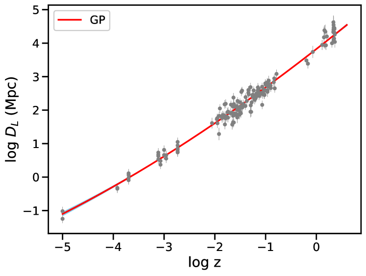
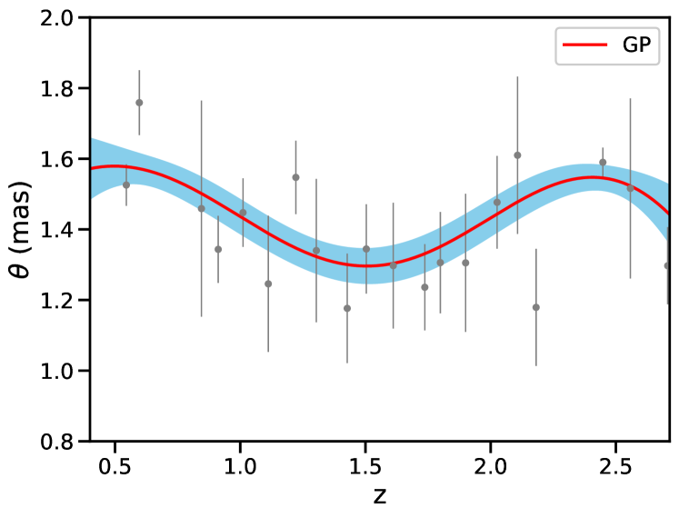
Figure 1: Top panel: The reconstructed function $\log D_{L,HII}(z)$ with corresponding $1\sigma$ errors by using GP (red line), and the gray dots dots with error bars represent measurements of HII regions; Bottom panel: The GP-reconstructed function $\theta(z)$ from compact radio sources observations.

Artificial Neural Network.— For the second nonparametric approach, we turn to Artificial Neural Network (ANN) and show the reconstructed function from observational data. With the development of computer hardware in the recent ten years, machine learning technology has been gradually applied to many research fields in astronomy, and shown excellent potential for solving cosmological problems, such as analyzing gravitational waves 40 ; 41 and constraining cosmological parameters 42 ; 43 ; 44 ; 45 ; 46 ; 47 .

The main purpose of an ANN is to construct an approximate function or map that correlates the input data with the output data. The ANN has been shown to be ”universal approximator” that can represent a wide variety of functions 48 ; 49 . The ANN is made up of neurons, which are very simple elements that receive digital input. Generally speaking, the artificial neural network consists of an input layer, one or more hidden layers and an output layer. Each layer takes a vector from the previous layer as input, applies a linear transformation and a nonlinear activation function to the input, and propagates the current result to the next layer. Formally, in a vectorized way 50

$$\mathbf{z_{i+1}}=\mathbf{x_{i}}W_{i+1}+\mathbf{b_{i+1}},$$ (7)

$$\mathbf{x_{i}}=f(\mathbf{z_{i+1}}),$$ (8)

where $\mathbf{x_{i}}$ is the input vector at the $i$th layer, $W_{i+1}$ and $\mathbf{b_{i+1}}$ are linear weights matrix and the offset vector which need to be optimized, $\mathbf{z_{i+1}}$ is the output vector after linear transformation, and $f$ is the activation function. Here, the Exponential Linear Unit (ELU) is acted as the activation function 51 , which is given by

$$f(x)=\begin{cases}x&x>0\\ \alpha(\exp(x)-1)&x\leq 0\end{cases}\quad,$$ (9)

where $\alpha$ denotes the hyper-parameter that controls the value to which an ELU saturates for negative net inputs. Compared to other activation functions (such as the rectified linear and the leaky rectified linear), when the network exceeds five layers, ELU can not only improve the learning speed, but also have better generalization performance 51 .

The ANN equals to a function $f_{W,\mathbf{b}}(\mathbf{x})$. The goal of ANN is to make its output to be as close as possible to the target value $\mathbf{y}$. Then, according to the difference between the predicted value $f_{W,\mathbf{b}}(\mathbf{x})$ of the current network and the target value $\mathbf{y}$, the weight matrix of each layer needs to be constantly updated for minimize the difference, which is defined by a loss function $\mathcal{L}$. The method used is gradient descent, that is, by constantly moving the loss value to the opposite direction of the current corresponding gradient to reduce the loss value. Formally, in a vectorized way 52

$$\frac{\partial\mathcal{L}}{\partial x_{i+1}} =f^{\prime}(x_{i+1})\frac{\partial\mathcal{L}}{\partial x_{i+1}},$$

$$\frac{\partial\mathcal{L}}{\partial W_{i+1}} =x_{i}^{T}\frac{\partial\mathcal{L}}{\partial z_{i+1}},$$

$$\frac{\partial\mathcal{L}}{\partial x_{i}} =W_{i+1}^{T}\frac{\partial\mathcal{L}}{\partial z_{i+1}},$$

$$\frac{\partial\mathcal{L}}{\partial{b}_{i+1}} =\left(\frac{\partial\mathcal{L}}{\partial z_{i+1}}\right),$$ (10)

where the operator $\partial$ denotes partial derivatives, and $f^{\prime}$ is the derivative for the nonlinear function $f$.

According to the publicly released code by the work 50 , which explicitly describe the ANN method, we use the module called Reconstruct Functions with ANN (ReFANN) to perform the reconstruction of the HII regions and radio quasars data-sets. Similarly, we show the reconstructed function $\log D_{L,HII}(z)$ by using ANN method as a function of logarithmic redshift $\log z$ with the estimation of $1\sigma$ confidence region in the top panel of Fig. 2. For compact radio sources, the reconstructed function $\theta(z)$ with corresponding $1\sigma$ uncertainties by using ANN is given in the bottom panel of Fig. 2. Similarly, we also reconstruct 1000 points for HII regions and compact radio sources, respectively. Compared to GP technology, the ANN method does not assume random variables that satisfy the Gaussian distribution, which is a completely data driven approach. It is interestingly to note that the uncertainties of the data reconstructed by ANN are almost equal to that of the observations. Therefore, the $1\sigma$ confidence region reconstructed by ANN can be considered as the average level of observational error. We refer the reader to Ref. 46 for further details on this issue.

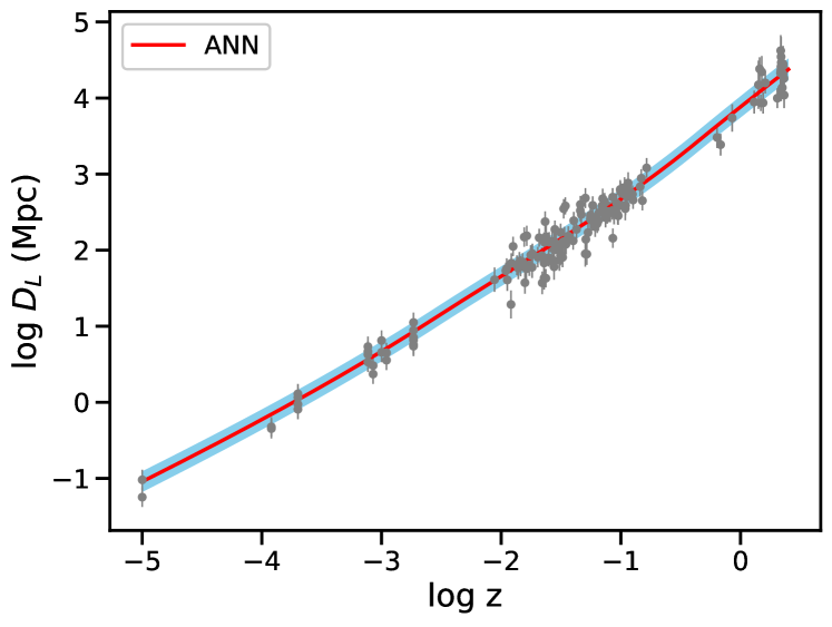
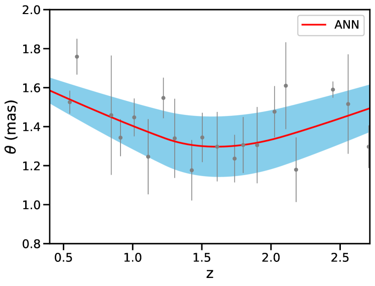
Figure 2: Top panel: The reconstructed function $\log D_{L,HII}(z)$ with $1\sigma$ errors by using ANN (red line), and the gray dots dots with error bars represent measurements of HII regions; Bottom panel: The reconstructed function $\theta(z)$ by using ANN from compact radio sources observations.

2.4 Testing the validity of CDDR

In order to test the validity of CDDR, we use the reconstructed data to directly perform a model-independent test of CDDR, i.e., we do not adopt any parameterized form to quantify the CDDR, which is given by the following form 53 ; 54

$$\eta(z)=\frac{D_{L}(z)}{D_{A}(z)(1+z)^{2}}.$$ (11)

Note that any statistically significant deviation from $\eta(z)=1$ could indicate possible violation of the three basic CDDR assumptions. Furthermore, we turn to four parameterized forms of CDDR, which have been extensively discussed in the quoted papers Cao11b

$$\eta_{th}(z,\eta_{j})=\left\{\begin{array}[]{l@{\hspace{1cm}}l}1+\eta_{0},\hfil\hskip 28.45274pt\\ 1+{\eta_{1}}z,\hfil\hskip 28.45274pt\\ 1+\eta_{2}z/(1+z),\hfil\hskip 28.45274pt\\ 1+\eta_{3}z+\eta_{4}z^{2}.\hfil\hskip 28.45274pt\\ \end{array}\right.$$ (12)

Note that the first parameterized form is independent of redshift, therefore we can compare it to other parameterized forms to check its possible dependency on the redshift. In general, $\eta(z)$ can be treated as parameterized functions of the redshift. In this work, we also use other general parametric representations for a possible redshift dependence of CDDR including two one-parameter expressions and a two-parameter parametrization. The consistency of the results under different parameterized forms will enhance the robustness of the conclusion.

From the observational perspective, we obtain the luminosity distance $D_{L}(z)$ through the ”$L$–$\sigma$” of HII galaxies and extragalactic HII regions, and the diameter distance $D_{A}(z)$ can be derived from compact structure in radio quasars. For a given $D_{L,HII}$ data point, the angular diameter distance $D_{A,QSO}$ should be observed at the same redshift. To avoid introducing additional systematic errors, a cosmological model-independent selection criterion is considered. We take $|z_{HII}-z_{QSO}|<0.005$ in our analysis 6 ; 7 . If one only consider the actual observational sample, it is difficult to achieve a rigorous CDDR test and get convincing results. That is the reason why we used two non-parameterized techniques mentioned above to reconstruct the data. Using the reconstructed samples, we are able to have a one-to-one matching between HII regions and compact structure in radio quasars . After executing the redshift selection criterion by using reconstructed data samples, 892 data are remained. Subsequently, the observed $\eta_{obs}(z)$ can be represented by following form

$$\eta_{obs}(z) = \frac{D_{L,HII}}{D_{A,QSO}(1+z)^{2}}$$

$$= \frac{\theta}{l_{m}(1+z)^{2}}10^{0.5[\alpha\log\sigma(\textrm{H}\beta)-\log F(\textrm{H}\beta)+\kappa]-25.04}.$$

Uncertainties have been assessed from the standard uncertainty propagation formula, based on (uncorrelated) uncertainties of observable quantities. The total uncertainty budget includes the ionized gas velocity dispersion $\sigma_{\log\sigma(\textrm{H}\beta)}$, flux density $\sigma_{\log F(\textrm{H}\beta)}$ and additional systematic errors introduced from the calibrations of $\alpha$ and $\kappa$ in HII regions data, the angular size $\sigma_{\theta}$, and additional systematic errors introduced in the calibrations of linear size $l_{m}$ in radio quasars. So the total uncertainty of $\eta_{obs}(z)$ can be expressed as

$$\sigma_{\eta_{obs}}=\sqrt{\sigma_{\log\sigma(\textrm{H}\beta)}^{2}+\sigma_{\log F(\textrm{H}\beta)}^{2}+\sigma_{\alpha}^{2}+\sigma_{\kappa}^{2}+\sigma_{\theta}^{2}+\sigma_{l_{m}}^{2}}.$$ (14)

In order to determine the best fitting CDDR parameters and corresponding uncertainties, we use the Bayesian statistical methods to obtain the posterior probability density function of the CDDR parameters $\eta_{j}$ ($j=0,..,4$) corresponding to four parametrization forms of Eq. (12). The posterior probability density function is given by

$$p(\mathbf{\eta}|obs\,\ data)\propto\mathcal{L}(\mathbf{\eta},obs\,\ data)\times p(\mathbf{\eta}),$$ (15)

where $\mathcal{L}$ is the likelihood function, and has a following form of

$$\mathcal{L}=\prod_{i}^{i=892}\frac{1}{\sqrt{2\pi}\sigma_{\eta}}{\rm exp}\left[-\frac{1}{2}\frac{(\eta_{obs}(z)-\eta_{th}(z,\eta_{j}))^{2}}{\sigma_{\eta}^{2}}\right],$$ (16)

and $p(\eta)$ is the prior, and assumed the following uniform distribution: $p(\eta_{j})=U[-1,1]$. We use the Python module $emcee$ 55 to perform the Markove Chain Monte Carlo (MCMC) analysis.

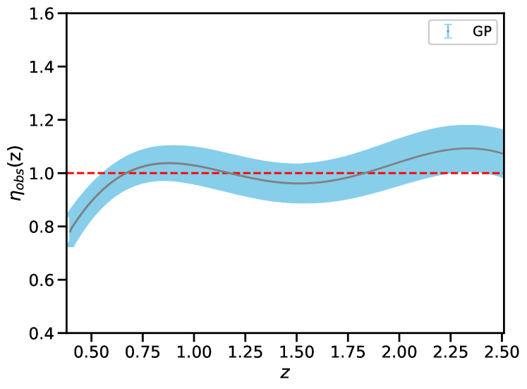
Figure 3: Cosmic distance duality relation $\eta(z)$ for the GP reconstruction from the HII galaxy and compact radio quasar sample. The dashed line at unity is $\eta(z)=1$, the solid line is the ANN fit, and the shaded region is the $1\sigma$ GP errors.

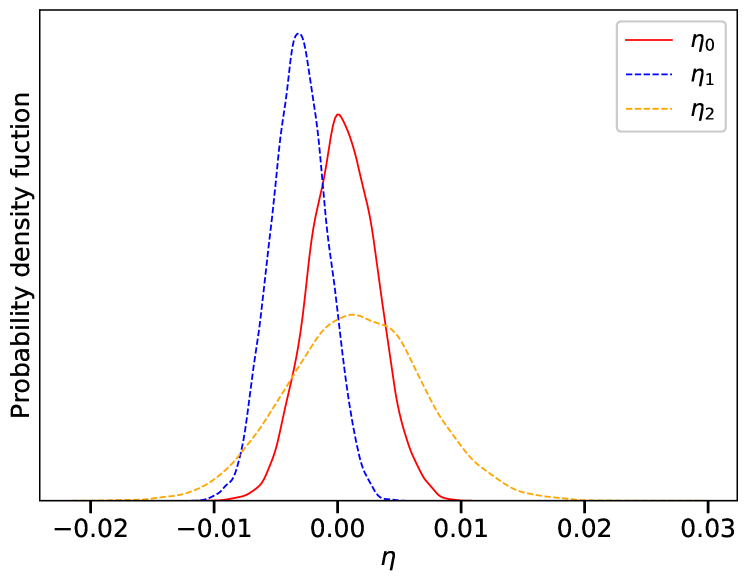
Figure 4: The posterior probability density function with three parameterized forms $\eta_{j}$ ($j=0,1,2$) by using GP reconstructed HII galaxy and compact radio quasar samples.

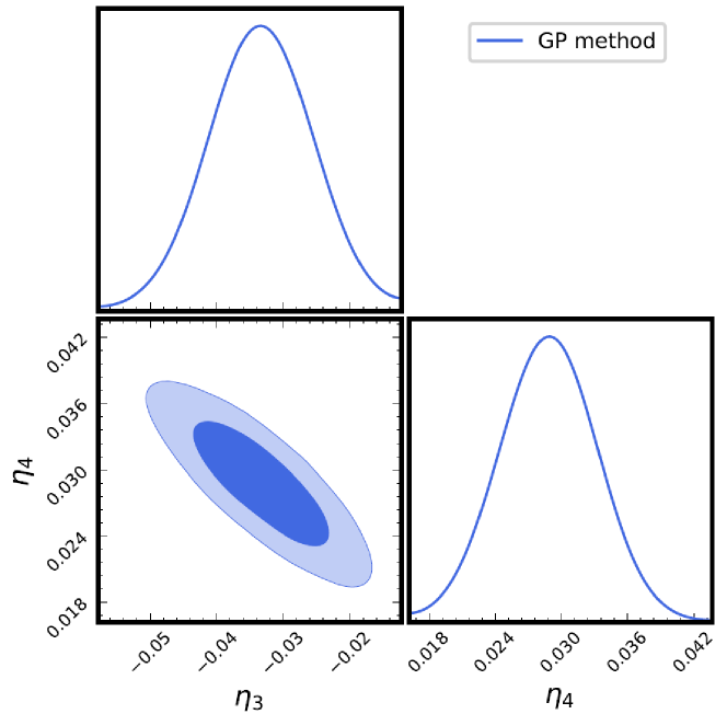
Figure 5: The 1D and 2D marginalized probability distributions for the fourth CDDR parameters $\eta_{3}$ and $\eta_{4}$ by using GP reconstructed HII galaxy and compact radio quasar samples.

3 Results and Discussion

$\eta_{j}$(z)+GP method	$\eta_{0}$	$\eta_{1}$	$\eta_{2}$	$\eta_{3}$	$\eta_{4}$
$1+\eta_{0}$	$0.001\pm 0.003$	$\Box$	$\Box$	$\Box$	$\Box$
$1+{\eta_{1}}z$	$\Box$	$-0.003\pm 0.003$	$\Box$	$\Box$	$\Box$
$1+\eta_{2}z/(1+z)$	$\Box$	$\Box$	$0.001\pm 0.005$	$\Box$	$\Box$
$1+\eta_{3}z+\eta_{4}z^{2}$	$\Box$	$\Box$	$\Box$	$-0.033\pm 0.006$	$0.029\pm 0.003$
$\eta_{j}$(z)+ANN method	$\eta_{0}$	$\eta_{1}$	$\eta_{2}$	$\eta_{3}$	$\eta_{4}$
$1+\eta_{0}$	$0.031\pm 0.016$	$\Box$	$\Box$	$\Box$	$\Box$
$1+{\eta_{1}}z$	$\Box$	$0.028\pm 0.014$	$\Box$	$\Box$	$\Box$
$1+\eta_{2}z/(1+z)$	$\Box$	$\Box$	$0.031\pm 0.033$	$\Box$	$\Box$
$1+\eta_{3}z+\eta_{4}z^{2}$	$\Box$	$\Box$	$\Box$	$0.033\pm 0.043$	$0.027\pm 0.025$

Table 1: Constraints on the CDDR parameters for four types of parameterized forms, in the framework of GP and ANN technologies.

Let’s start with the reconstruction of HII galaxy and radio quasar sample using GP. In Fig. 3 we show a particular realization of the reconstructed CDDR, along with the case of $\eta(z)=1$ (dashed green line) and the corresponding best-fit (solid colored line) for the GP. Our results indicate that there is no obvious deviation from $\eta(z)=1$ at $1\sigma$ confidence level. In the higher redshift region, due to the lack of observational data the errors of reconstruction become larger and the statistical significance of CDDR reconstruction is affected. Such finding is well consistent with that obtained in the recent works 12a ; 12b ; 12c ; 12d . Focusing on the different parameterized form of $\eta_{obs}(z)$, the numerical results by using GP reconstructed technology for three parameterized forms $\eta_{j}$ ($j=0,1,2$) are summarized in Table 1, and the posterior probability density functions are shown in Fig. 4. For the first parameterized form, the best fitting value with 1$\sigma$ error is $\eta_{0}=0.001\pm 0.0031$, which demonstrates that there is no evidence for the dependence relation between the CDDR parameter and redshift. Working on the second parameterized form, we obtain $\eta_{1}=-0.003\pm 0.003$, which contains zero value within $\sim 1.2\sigma$ confidence level. Considering the redshift coverage of our CDDR test ($z\sim 2.3$), the third parametrization may effectively avoid the possible divergence at high redshift. In this case, the best fitting value $\eta_{2}$ with 1$\sigma$ confidence level is $\eta_{2}=0.001\pm 0.005$. Meanwhile, for the two-parameter form, the graphic representation and numerical results of the constraints on the CDDR parameters ($\eta_{3}$, $\eta_{4}$) are shown in Fig. 5 and Table 1. One can clearly see that the CDDR seems to be violated at 1$\sigma$ confidence level, $\eta_{3}=-0.033\pm 0.006$ and $\eta_{4}=0.029\pm 0.003$. However, one should be noted that the degeneracy between $\eta_{3}$ and $\eta_{4}$ is strong, and they are in negative correlation. If $\eta_{3}$ increases to zero, then $\eta_{4}$ will go back to zero, which means that the strong degeneracy between them affects our test of CDDR validity. Such result, which is similar with the findings of previous works 8 , highlights the importance of choosing a reliable parametrization to describe $\eta(z)$ in the early universe. Benefit from the GP technology, the HII/QSO pairs satisfying the redshift selection criteria have a massive growth, therefore, a considerable amount of high-redshift samples ($z>1.4$) have been included in our analysis. Actually, such a combination of HII regions and radio quasars enables us to get more precise measurements at the level of $\Delta\eta\sim 10^{-3}$ by using GP reconstructed technology. Our method provided constraints for testing validity of CDDR more stringent than other currently available results based on real observational data.

We also consider the added benefit on the reconstruction brought by other machine learning methods. Working on the reconstructed luminosity and angular diameter distances with ANN, we obtain the reconstruction of the distance duality relation $\eta(z)$ in Fig. 6, when the full data combination of HII galaxies and compact radio quasar is considered. Similarly, the reconstructed $\eta(z)$ function is compatible with the validity of CDDR at the 1$\sigma$ confidence level, hence there is no clear deviation from such fundamental relation in modern cosmology. Furthermore, for both ML approaches we find that the reconstructed errors are inconsistent with each other, since the GP and the ANN are in principle rather different reconstruction methods. Next, in Table 1 we show the numerical result for CDDR parameters in the framework of four parameterized forms. The posterior probability density functions of CDDR parameters $\eta_{j}$ ($j=0,1,2$) from reconstructed HII galaxy and radio quasar samples are shown in Fig. 7. We find that there is some deviation from CDDR at 1$\sigma$ confidence level. The best fitting values $\eta_{0}$ and $\eta_{1}$ are $0.031\pm 0.016$ and $0.028\pm 0.014$ for first and second parameterized forms, but the results are still consistent with zero CDDR parameters within $2\sigma$ confidence level. Meanwhile, for the third parameterized form, we get $\eta_{2}=0.031\pm 0.033$ with 1$\sigma$ uncertainty. Considering the forth form, the results are $\eta_{3}=0.033\pm 0.043$ and $\eta_{4}=0.027\pm 0.025$ with 1$\sigma$ errors and shown in Fig. 8. Although considering more parameters would make the constrained precision of the CDDR parameters worse, our findings also demonstrate the robustness of CDDR validity in two-parameter form. In general, whatever parameterized forms are considered here, our results indicate that there is no large extent violation of the CDDR validity at the current observational data level, and this is one of unambiguity conclusions in our work.

In order to highlight the potential of our method, it is necessary to compare our results with those obtained in the previous works. Traditionally, the angular diameter distances are derived from SZ effect of galaxy clusters 5 ; 6 , BAOs 4 , GRBs 56 , and SGLs 7 ; 8 . One can combine the luminosity distance obtained from SN Ia observations to test the validity of CDDR. Our results are consistent with the findings of their previous works, which confirm the validity of the CDDR at early Universe. However, the angular diameter distances inferred from SZ effect and BAOs are model dependent, SGLs need to the assumption of a flat Universe, and GRBs requires additional external calibrators to calibrate it at low redshifts. We remark here that, without any assumptions, the angular diameter distances estimated from compact structure in radio quasars provides a new possibility to test the fundamental relations in the early universe model independently. More importantly, in work of 54 , they simulated gravitational wave (GW) observations based on third-generation GW detectors Einstein Telescope and simulated radio quasars from VLBI to test the CDDR. Their results shown that the CDDR parameter $\Delta\eta_{0}\sim 0.0029$, $\Delta\eta_{1}\sim 0.0018$, and $\Delta\eta_{2}\sim 0.0051$ (at 68.3% confidence level) corresponding to first, second and third parameterized forms in our work. However, we should seek other methods and technologies until the observed GW events based on the third-generation GW detectors will be sufficient to get statistical results in the future.

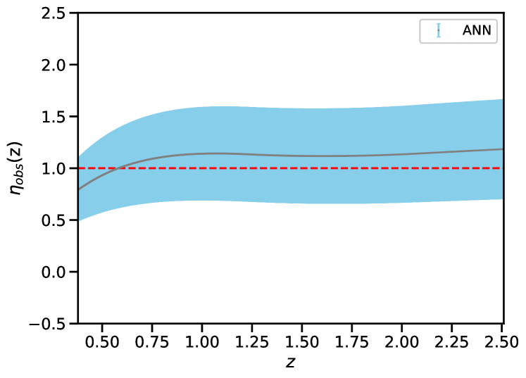
Figure 6: Cosmic distance duality relation $\eta(z)$ for the ANN reconstruction from the HII galaxy and compact radio quasar sample. The dashed line at unity is $\eta(z)=1$, the solid line is the ANN fit, and the shaded region is the $1\sigma$ ANN errors.

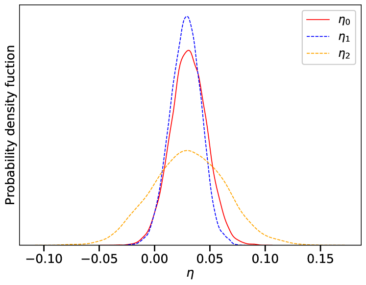
Figure 7: The posterior probability density function with three parameterized forms $\eta_{j}$ ($j=0,1,2$) by using ANN reconstructed HII galaxy and compact radio quasar samples.

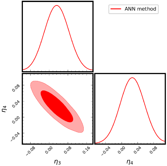
Figure 8: The 1D and 2D marginalized probability distributions for the fourth CDDR parameters $\eta_{3}$ and $\eta_{4}$ by using ANN reconstructed HII galaxy and compact radio quasar samples.

4 Conclusion

The cosmic distance duality relation (CDDR), as a fundamental relation based on the metric theory of gravity, plays a important role in modern cosmology. Possible violations of such fundamental relation indicates that the non-conservation of the photon number from the source to the observer due to some new physics. In this paper, we have proposed a new model-independent method to test the CDDR with the latest observations of HII galaxies acting as standard candles and ultra-compact structure in radio quasars acting as standard rulers. Specially, two machine learning reconstruction methods, i.e., Gaussian Process (GP) and Artificial Neural Network (ANN), are respectively applied to reconstruct the Hubble diagrams from the observed HII galaxy and radio quasar samples. In order to enhance the robustness of the final results, we use four commonly used parameterized forms $\eta=1+\eta_{0},\eta=1+{\eta_{1}}z,\eta=1+\eta_{2}z/(1+z)$, and $\eta=1+\eta_{3}z+\eta_{4}z^{2}$ to describe the possible violation of CDDR. Meanwhile, we also exploit a fully agnostic reconstruction of CDDR based on two machine learning methods, which allows us to obtain constraints without any assumption on the redshift trend of possible deviations from CDDR.

First of all, we focus on the reconstruction of HII regions and compact radio quasar samples through the GP method. Based on the reconstructed standard candle and standard ruler data, we obtain the best-fit values of the CDDR parameters $\eta_{0}=0.001\pm 0.0031$, $\eta_{1}=-0.0031\pm 0.0027$, and $\eta_{2}=0.0014\pm 0.0054$ for the three one-parameter forms, which are well consistent with no violation of the cosmic distance duality relation. The results suggest that the tests of cosmic opacity are not significantly sensitive to the parametrization for $\eta$. For the two-parameter parameterization, we obtain $\eta_{3}=-0.033\pm 0.006$ and $\eta_{4}=0.029\pm 0.003$ at 68.3$\%$ confidence level. A strong degeneracy between the two redshift-dependent CDDR parameters is also revealed in this analysis. Note that although such negative correlation could potentially affect our test of CDDR, the validity of such fundamental relation is still supported within $2.8\sigma$. Therefore, our results indicate that there is no obvious violation of the CDDR at the current observational data level, based on Gaussian Process for the overlapping redshift domain ($z\sim 2.3$). Moreover, we find that ultra-compact radio quasars provide an alternative to the use of HII galaxies to confirm the validity of the CDDR, reaching $10^{-3}$ constraints on the violation parameter.

It is still interesting to see whether those conclusions may be changed with a different machine learning reconstruction method. Working on the reconstructed HII regions and compact radio quasar samples with ANN, one could derive robust constraints on the violation parameter at the precision of $10^{-2}$, with the validity of such distance duality relation within $2\sigma$. Although not all of the parameterized forms support the validity of CDDR within 1$\sigma$ in the framework of GP, more convincing results are obtained in the ANN method. Although the GP and ANN methods have their own advantages and disadvantages 50 , they both show great potential in the studies of precision cosmology. In the case of non-parameterized reconstruction of CDDR, our results based on the two machine learning methods both support that there is no obvious deviation from $\eta(z)=1$ within $1\sigma$ confidence level. However, the statistical significance of our CDDR reconstruction is still significantly affected by the lack of observational data, especially at higher redshifts. Looking to the future, an increase in the number of high-redshift standard probes would improve the precision of our approach even further. This strengthens our interest in observational search for more HII galaxies and compact radio quasars with smaller statistical and systematic uncertainties.

As a final remark, any possible deviation the CDDR might have profound implications for the understanding of fundamental physics and natural laws. Therefore, our results highlight the importance of machine learning in accurately testing the current pillars of modern cosmology and probing new physics beyond the standard cosmological model. Summarizing, considering the wealth of available data and various machine learning technologies in the future, we may be optimistic to expect detecting possible deviation from the CDDR at much higher precision.

Data Availability

This manuscript has associated data in a data repository. The data underlying this paper will be shared on reasonable request to the corresponding author.

References

- (1) I. M. H. Etherington, Phil. Mag 15, 761 (1933)
- (2) I. M. H. Etherington, Gen. Relativ. Gravit 39, 1055 (2007)
- (3) Planck Collaboration (2018). arXiv:1807.06209
- (4) S. Cao, Z.-H. Zhu, SCPMA 54, 12 (2011)
- (5) S. Cao, M. Biesiada, X. Zheng, Z.-H. Zhu, MNRAS 457, 281 (2016)
- (6) P. X. Wu, Z. X. Li, H. Yu, PRD 92, 023520 (2015)
- (7) R. F. L. Holanda, J. A. S. Lima, M. B. Ribeiro, ApJL 722, L233 (2010)
- (8) S. Cao, N. Liang, RAA 11, 1199 (2011)
- (9) Z. X. Li, P. X. Wu, H. W. Yu, ApJL 729, L14 (2011)
- (10) K. Liao, Z. X. Li, S. Cao, et al., ApJ 822, 74 (2016)
- (11) C. Z. Ruan, F. Melia, T. J. Zhang, ApJ 866, 31 (2018)
- (12) A. G. Riess, L. M. Macri, S. L. Hoffmann, et al., ApJ 826, 56 (2016)
- (13) H. Yu, F. Y. Wang, ApJ 828, 85 (2016)
- (14) M. Z. Lv, J.-Q. Xia, Phys. Dark Universe 13, 139 (2016)
- (15) V. F. Cardone, S. Spiro, I. Hook, R. Scaramella, PRD 85, 123510 (2012)
- (16) X. G. Zheng, K. Liao, M. Biesiada, et al. ApJ 892, 103 (2021)
- (17) R. Arjona, H. N. Lin, S. Nesseris, L. Tang, PRD 103, 103513 (2021)
- (18) N. B. Hogg, M. Martinelli, S. Nesseris, JCAP 12, 019 (2020)
- (19) P. Mukherjee, A. Mukherjee, MNRAS 504, 3938 (2021)
- (20) M. Martinelli, C. J. A. P. Martins, S. Nesseris, et al., A&A 644, A80 (2020)
- (21) G. Risaliti, E. Lusso, Nat. Astron 3, 272 (2019)
- (22) T. H. Liu, S. Cao, M. Biesiada, et al., ApJ 899, 71 (2020)
- (23) T. H. Liu, S. Cao, J. Zhang, et al., MNRAS 496, 708 (2020)
- (24) S. Cao, X. G. Zheng, M. Biesiada, et al., A&A 606, A15 (2017)
- (25) B. Paczynski, ApJ 308, 43 (1986)
- (26) R. Terlevich, J. Melnick, MNRAS 195, 839, (1981)
- (27) R. Terlevich, E. Terlevich, J. Melnick, et al., MNRAS 451, 3001 (2015)
- (28) J. J. Wei, X. F. Wu, F. Melia, MNRAS 463, 1144 (2016)
- (29) J. Melnick, M. Moles, R. Terlevich, J. M. Garcia-Pelayo, MNRAS 226, 849 (1987)
- (30) M. Plionis, R. Terlevich, S. Basilakos, et al., MNRAS 416, 2981 (2011)
- (31) D. Mania & B. Ratra, PLB 715, 9 (2012)
- (32) Y. Wu, S. Cao, J. Zhang, et al., ApJ 888, 113 (2020)
- (33) K. I. Kellermann, Nature 361, 134 (1993)
- (34) L. Gurvits, ApJ 425, 442 (1994)
- (35) A. R. Preston, et al., AJ 90, 1599 (1985)
- (36) X. L. Li, S. Cao, X. G. Zheng, et al., EPJC 77, 677 (2017)
- (37) J. Z. Qi, S. Cao, M. Biesiada, et al., EPJC 77, 502 (2017)
- (38) Y. B. Ma, J. Zhang, S. Cao, et al., EPJC 77, 891 (2017)
- (39) T. Xu, S. Cao, J. Z. Qi, et al., JCAP 06, 042 (2018)
- (40) S. Cao, M. Biesiada, J. Jackson, et al., JCAP 02, 012 (2017)
- (41) S. Cao, M. Biesiada, X. G. Zheng, et al., EPJC 78, 749 (2018)
- (42) M. Seikel, C. Clarkson, M. Smith, JCAP 6, 036 (2012)
- (43) M. Seikel, S. Yahya, R. Maartens, C. Clarkson, PRD 86, 083001 (2012)
- (44) T. Yang, Z. K. Guo, R.G. Cai, PRD 91, 123533 (2015)
- (45) R. Cai, Z. K. Guo, T. Yang, PRD 93, 043517 (2016)
- (46) T. H. Liu, S. Cao, J. Zhang, et al., ApJ 886, 94 (2019)
- (47) F. Melia, M. K. Yennapureddy, JCAP 02, 034 (2018)
- (48) M. K. Yennapureddy, & F. Melia, EPJC 78, 258 (2018)
- (49) E. Ó. Colgáin, M. M. Sheikh-Jabbari, arXiv: 2101.08565
- (50) S. Dhawan, J. Alsing, S. Vagnozzi, MNRAS 506, L1 (2021)
- (51) M. K. Yennapureddy, F. Melia, JCAP 11, 029 (2017)
- (52) C. Z. Ruan, F. Melia, T. J. Zhang, ApJ 866, 31 (2018)
- (53) X. Li, W. Yu, X. Fan, arXiv:1712.00356
- (54) D. George, E. A. Huerta, PRD 97, 044039 (2018)
- (55) J. Fluri, T. Kacprzak, A. Lucchi, et al., PRD 98, 123518 (2018)
- (56) J. Fluri, T. Kacprzak, A. Lucchi, et al., PRD 100, 063514 (2019)
- (57) M. Ntampaka, D.J. Eisenstein, S. Yuan, L.H. Garrison, arXiv:1909.10527
- (58) D. Ribli, B.Á. Pataki, J. M. Z. Matilla, et al., MNRAS 490, 1843 (2019)
- (59) G. J. Wang, S. Y. Li, J.Q. Xia, ApJS 249, 25 (2020)
- (60) G. J. Wang, X. J. Ma, J.Q. Xia, MNRAS 501, 5714 (2021)
- (61) G. Cybenko, Math. Control Signal Syst 2, 303 (1989)
- (62) K. Hornik, NN 4, 251 (1991)
- (63) G. J. Wang, X. J. Ma, S. Y. Li, J.Q. Xia, ApJS 246, 13 (2020)
- (64) D. A. Clevert, T. Unterthiner, S. Hochreiter, arXiv:1511.07289
- (65) Y. LeCun, L. Bottou, G. B. Orr, K. R. Müller, Neural Networks: Tricks of the Trade https://nyuscholars.nyu.edu/en/publications/efficientbackprop (2012)
- (66) X. G. Zheng, K. Liao, M. Biesiada, et al., ApJ 892, 103 (2020)
- (67) J.Z. Qi, S. Cao, C. F. Zheng, et al., PRD 99, 063507 (2019)
- (68) D. Foreman-Mackey, D. W. Hogg, D. Lang, J. Goodman, PASA 125, 306 (2013)
- (69) R. F. L. Holanda, V. C. Busti, F. S. Lima, J. S. Alcaniz, JCAP 09, 039 (2017)