Information-Theoretic Characterization of the Generalization Error for Iterative Semi-Supervised Learning

Abstract

Using information-theoretic principles, we consider the generalization error (gen-error) of iterative semi-supervised learning (SSL) algorithms that iteratively generate pseudo-labels for a large amount of unlabelled data to progressively refine the model parameters. In contrast to most previous works that bound the gen-error, we provide an exact expression for the gen-error and particularize it to the binary Gaussian mixture model. Our theoretical results suggest that when the class conditional variances are not too large, the gen-error decreases with the number of iterations, but quickly saturates. On the flip side, if the class conditional variances (and so amount of overlap between the classes) are large, the gen-error increases with the number of iterations. To mitigate this undesirable effect, we show that regularization can reduce the gen-error. The theoretical results are corroborated by extensive experiments on the MNIST and CIFAR datasets in which we notice that for easy-to-distinguish classes, the gen-error improves after several pseudo-labelling iterations, but saturates afterwards, and for more difficult-to-distinguish classes, regularization improves the generalization performance.

Keywords: Generalization error, Semi-supervised learning, Pseudo-label, Information theory, Binary Gaussian mixture.

1 Introduction

In real-life machine learning applications, it is relatively easy and inexpensive to obtain large amounts of unlabelled data, while the number of labelled data examples is usually small due to the high cost of annotating them with true labels. In light of this, semi-supervised learning (SSL) has come to the fore (Chapelle et al., 2006; Zhu, 2008; Van Engelen and Hoos, 2020). SSL makes use of the abundant unlabelled data to augment the performance of learning tasks with few labelled data examples. This has been shown to outperform supervised and unsupervised learning under certain conditions. For example, in a classification problem, the correlation between the additional unlabelled data and the labelled data may help to enhance the accuracy of classifiers. Among the plethora of SSL methods, pseudo-labelling (Lee, 2013) has been observed to be a simple and efficient way to improve the generalization performance empirically. In this paper, we consider the problem of pseudo-labelling a subset of the unlabelled data at each iteration based on the previous output parameter and then refining the model progressively, but we are interested in analysing this procedure theoretically. Our goal in this paper is to understand the impact of pseudo-labelling on the generalization error.

A learning algorithm can be viewed as a randomized map from the training dataset to the output model parameter. The output is highly data-dependent and may suffer from overfitting to the given dataset. In statistical learning theory, the generalization error (gen-error), or generalization bias, is defined as the expected gap between the test and training losses, and is used to measure the extent to which the algorithms overfit to the training data (Russo and Zou, 2016; Xu and Raginsky, 2017; Kawaguchi et al., 2017). In SSL problems, the unlabelled data are expected to improve the generalization performance in a certain manner and thus, it is a worthy endeavor to investigate the behaviour theoretically. Although there exist many works studying the gen-error for supervised learning problems, the gen-error of SSL algorithms is yet to be explored.

1.1 Related Works

The extensive literature review is categorized into three aspects.

Semi-supervised learning:

There have been many existing results discussing about various methods of SSL. The book by Chapelle et al. (2006) presented a comprehensive overview of the SSL methods both theoretically and practically. Chawla and Karakoulas (2005) presented an empirical study of various SSL techniques on a variety of datasets and investigated sample-selection bias when the labelled and unlabelled data are from different distributions. Zhu (2008) partitioned SSL methods into six main classes: generative models, low-density separation methods, graph-based methods, self-training and co-training. Pseudo-labelling is a technique among the self-training and co-training (Zhu and Goldberg, 2009). In self-training, the model is initially trained by the limited number of labelled data and generate pseudo-labels to the unlabelled data. Subsequently, the model is retrained with the pseudo-labelled data and repeats the process iteratively. It is a simple and effective SSL method without restrictions on the data samples (Triguero et al., 2015). A variety of works have also shown the benefits of utilizing the unlabelled data. Singh et al. (2008) developed a finite sample analysis that characterized how the unlabelled data improves the excess risk compared to the supervised learning, with respect to the number of unlabelled data and the margin between different classes. Li et al. (2019) studied multi-class classification with unlabelled data and provided a sharper generalization error bound using the notion of Rademacher complexity that yields a faster convergence rate. Zhu (2020) considered the general SSL setting by assuming the loss function to be $\beta$-exponentially concave or the $0$-$1$ loss, and used a Bayesian method for prediction instead of empirical risk minimization which we consider. The author presented an upper bound for the excess risk and the learning rate in terms of the number of labelled and unlabelled data examples. Carmon et al. (2019) proved that using unlabelled data can help to achieve high robust accuracy as well as high standard accuracy at the same time. Dupre et al. (2019) considered iteratively pseudo-labelling the whole unlabelled dataset with a confidence threshold and showed that the accuracy converges relatively quickly. Oymak and Gülcü (2021), in which part of our analysis hinges on, studied SSL under the binary Gaussian mixture model setup and characterized the correlation between the learned and the optimal estimators concerning the margin and the regularization factor. Recently, Aminian et al. (2022) considered the scenario where the labelled and unlabelled data are not generated from the same distribution and these distributions may change over time, exhibiting so-called covariate shifts. They provided an upper bound for the gen-error and proposed the Covariate-shift SSL (CSSL) method which outperforms some previous SSL algorithms under this setting. However, these works do not investigate how the unlabelled data affects the generalization error over the iterations.

Generalization error bounds:

The traditional way of analyzing generalization error involves using the Vapnik–Chervonenkis or VC dimension (Vapnik, 2000) and the Rademacher complexity (Boucheron et al., 2005). Recently, Russo and Zou (2016) proposed using the mutual information between the estimated output of an algorithm and the actual realized value of the estimates to analyze and bound the bias in data analysis, which can be regarded equivalent to the generalization error. This new approach is simpler and can handle a wider range of loss functions compared to the abovementioned methods and other methods such as differential privacy. It also paves a new way to improving generalization capability of learning algorithms from an information-theoretic viewpoint. Following Russo and Zou (2016), Xu and Raginsky (2017) derived upper bounds on generalization error of learning algorithms with mutual information between the input dataset and the output hypothesis, which formalizes the intuition that less information that a learning algorithm can extract from training dataset leads to less overfitting. Later Pensia et al. (2018) derived generalization error bounds for noisy and iterative algorithms and the key contribution is to bound the mutual information between input data and output hypothesis. Negrea et al. (2019) improved mutual information bounds for Stochastic Gradient Langevin Dynamics (SGLD) via data-dependent estimates compared to distribution-dependent bounds.

However, one major shortcoming of the aformentioned mutual information bounds is that the bounds go to infinity for (deterministic) learning algorithms without noise, e.g., Stochastic Gradient Descent (SGD). Some other works have tried to overcome this problem. Lopez and Jog (2018) derived upper bounds on the generalization error using the Wasserstein distance involving the distributions of input data and output hypothesis, which are shown to be tighter under some natural cases. Esposito et al. (2021) derived generalization error bounds via Rényi-, $f$-divergences and maximal leakage. Steinke and Zakynthinou (2020) proposed using the Conditional Mutual Information (CMI) to bound the generalization error; the CMI is useful as it possesses the chain rule property. Bu et al. (2020) provided a tightened upper bound based on the individual mutual information (IMI) between the individual data sample and the output. Wu et al. (2020) extended Bu et al. (2020)’s result to transfer learning problems and characterized the upper bound based on IMI and KL-divergence. In a similar manner, Jose and Simeone (2021) provided a tightened bound on transfer generalization error based on the Jensen–Shannon divergence. Moreover, recently, Aminian et al. (2021) and Bu et al. (2022) recently derived the exact characterization of gen-error for supervised learning and transfer learning with the Gibbs algorithm.

Regularization is an important technique to reduce the model variance (Anzai, 2012), but there are few works that theoretically analyse the relationship between the gen-error and regularization. Moody (1992) characterized the gen-error as a function of the regularization parameter in supervised nonlinear learning systems and showed that the gen-error decreases as the parameter increases. Bousquet and Elisseeff (2002) provided a stability-based gen-error upper bound in terms of the regularization parameter in supervised learning. Mignacco et al. (2020) studied how the regularization affects the expected accuracy in high-dimensional GMM supervised classification problem.

Gaussian mixture models (GMM):

The GMM is a popular, simple but non-trivial model that has been studied by many researchers. The performance of GMM classification problems depends on the data structure. The classical work of Castelli and Cover (1996) studied the classification problem in a binary mixture model with known conditional distributions but unknown mixing parameter and characterized the relative value of labelled and unlabelled data in improving the convergence rate of classification error probability. Akaho and Kappen (2000) characterized the generalization bias of general GMMs in supervised learning and discussed its dependency on data noise. Watanabe and Watanabe (2006) considered GMM in Bayesian learning and provided bounds for variational stochastic complexity. Wang and Thrampoulidis (2022) and Muthukumar et al. (2021) studied the dependence of the bGMM classification performance (using the $0$-$1$ loss) on the structure of data covariance by considering SVM and linear interpolation.

However, all these aforementioned works do not investigate the generalization performance of SSL algorithms.

1.2 Contributions

Our main contributions are as follows.

1. In Section 3, we leverage results by Bu et al. (2020) and Wu et al. (2020) to derive an information-theoretic gen-error bound at each iteration for iterative SSL; see Theorem 2.A. Moreover, in contrast to most previous works that bound the gen-error, we derive an exact characterization of gen-error at each iteration for negative log-likelihood (NLL) loss functions (see Theorem 2.B).

2. In Section 4, we particularize Theorem 2.B to the binary Gaussian mixture model (bGMM) with in-class variance $\sigma^{2}$. We show that for any fixed number of data samples, there exists a critical value $\sigma_{0}$ such that when the data variance (representing the overlap between classes) $\sigma^{2}<\sigma_{0}^{2}$, the gen-error decreases in the iteration count $t$ and converges quickly with a sufficiently large amount of unlabelled data. When $\sigma^{2}>\sigma_{0}^{2}$, the gen-error increases instead, which means using the unlabelled data does not help to reduce the gen-error across the SSL iterations. The empirical gen-error corroborates the theoretical results, which suggests that the characterization serves as a useful rule-of-thumb to understand how the gen-error changes across the SSL iterations and it can be used to establish conditions under which unlabelled data can help in terms of generalization.

3. In Section 5, we theoretically and empirically show that for difficult-to-classify problems with large overlap between classes, regularization can effectively help to mitigate the undesirable increase of the gen-error across the SSL iterations.

4. In Section 6, we implement the pseudo-labelling procedure on the MNIST and CIFAR datasets with few labelled data and abundant unlabelled data. The experimental results corroborate the phenomena for the bGMM that the gen-error decreases quickly in the early pseudo-labelling iterations and saturates thereafter for easy-to-distinguish classes but increases for hard-to-distinguish classes. By adding $\ell_{2}$-regularization to the hard-to-distinguish problem, we also observe improvements to the gen-error similar to that for the bGMM.

2 Problem Setup

Let the instance space be $\mathcal{Z}=\mathcal{X}\times\mathcal{Y}\subset\mathbb{R}^{d+1}$, the model parameter space be $\Theta$ and the loss fucntion be $l:\mathcal{Z}\times\Theta\to\mathbb{R}$, where $d\in\mathbb{N}$. We are given a labelled training dataset $S_{\mathrm{l}}=\{Z_{1},\ldots,Z_{n}\}=\{(X_{i},Y_{i})\}_{i=1}^{n}$ drawn from $\mathcal{Z}$, where each $Z_{i}=(X_{i},Y_{i})$ is independently and identically distributed (i.i.d.) from $P_{Z}=P_{X,Y}\in\mathcal{P}(\mathcal{Z})$. For any $i\in[n]$, $X_{i}$ is a vector of features and $Y_{i}$ is a label indicating the class to which $X_{i}$ belongs. However, in many real-life machine learning applications, we only have a limited number of labelled data while we have access to a large amount of unlabelled data, which are expensive to annotate. Then we can incorporate the unlabelled training data together with the labelled data to improve the performance of the model. This procedure is called semi-supervised learning (SSL). We are given an independent unlabelled training dataset $S_{\mathrm{u}}=\{X^{\prime}_{1},\ldots,X^{\prime}_{\tau m}\},\tau\in\mathbb{N}$, where each $X^{\prime}_{i}$ is generated i.i.d. from $P_{X}\in\mathcal{P}(\mathcal{X})$. Typically, $m\gg n$.

In the following, we consider the iterative self-training with pseudo-labelling in SSL setup, as shown in Figure 1. Let $t\in[0:\tau]$ denote the iteration count. In the initial round ($t=0$), the labelled data $S_{\mathrm{l}}$ are first used to learn an initial model parameter $\theta_{0}\in\Theta$. Next, we split the unlabelled dataset $S_{\mathrm{u}}$ into $\tau$ disjoint equal-size sub-datasets $\{S_{\mathrm{u},k}\}_{k=1}^{\tau}$, where $S_{\mathrm{u},k}=\{X^{\prime}_{(k-1)m+1},\ldots,X^{\prime}_{km}\}$. In each subsequent round $t\in[1:\tau]$, based on $\theta_{t-1}$ trained from the previous round, we use a predictor $f_{\theta_{t-1}}:\mathcal{X}\mapsto\mathcal{Y}$ to assign a pseudo-label $\hat{Y}^{\prime}_{i}$ to the unlabelled sample $X^{\prime}_{i}$ for all $i\in\mathcal{I}_{t}:=\{(t-1)m,(t-1)m+1,\ldots,tm\}$. Let $\hat{S}_{\mathrm{u},t}=\{(X_{i}^{\prime},\hat{Y}_{i}^{\prime})\}_{i\in\mathcal{I}_{t}}$ denote the $t^{\mathrm{th}}$ pseudo-labelled dataset. After pseudo-labelling, both the labelled data $S_{\mathrm{l}}$ and the pseudo-labelled data $\hat{S}_{\mathrm{u},t}$ are used to learn a new model parameter $\theta_{t}$. The procedure is then repeated iteratively until the maximum number of iterations $\tau$ is reached.

Figure 1: Paradigm of iterative self-training with pseudo-labelling in SSL

This setup is a classical and widely-used model in the realm of self-training in SSL (Chapelle et al., 2006; Zhu, 2008; Zhu and Goldberg, 2009; Lee, 2013), where in each iteration, only a subset of the unlabelled data are used. Furthermore, as discussed by Arazo et al. (2020), this method is less likely to overfit to incorrect pseudo-labels, compared to using all the unlabelled data in each iteration (also see Figure 10). Under this setup of iterative SSL, during each iteration $t$, our goal is to find a model parameter $\theta_{t}\in\Theta$ that minimizes the population risk with respect to the underlying data distribution

$$L_{P_{Z}}(\theta_{t}):=\mathbb{E}_{Z\sim P_{Z}}[l(\theta_{t},Z)].$$ (1)

Since $P_{Z}$ is unknown, $L_{P_{Z}}(\theta_{t})$ cannot be computed directly. Hence, we instead minimize the empirical risk. The procedure is termed empirical risk minimization (ERM). For any model parameter $\theta_{t}\in\Theta$, the empirical risk of the labelled data is defined as

$$L_{S_{\mathrm{l}}}(\theta_{t}):=\frac{1}{n}\sum_{i=1}^{n}l(\theta_{t},Z_{i}),$$ (2)

and for $t\geq 1$, the empirical risk of pseudo-labelled data $\hat{S}_{\mathrm{u},t}$ as

$$L_{\hat{S}_{\mathrm{u},t}}(\theta_{t}):=\frac{1}{m}\sum_{i\in\mathcal{I}_{t}}l(\theta_{t},(X_{i}^{\prime},\hat{Y}_{i}^{\prime})).$$ (3)

We set $L_{\hat{S}_{\mathrm{u},t}}(\theta_{t})=0$ for $t=0$. For a fixed weight $w\in[0,1]$, the total empirical risk can be defined as the following linear combination of $L_{S_{\mathrm{l}}}(\theta_{t})$ and $L_{\hat{S}_{\mathrm{u},t}}(\theta_{t})$:

$$L_{S_{\mathrm{l}},\hat{S}_{\mathrm{u},t}}(\theta_{t}) :=wL_{S_{\mathrm{l}}}(\theta_{t})+(1-w)L_{\hat{S}_{\mathrm{u},t}}(\theta_{t}).$$ (4)

In the usual case where the algorithm minimizes the average of the empirical training losses, one should set $w=\frac{n}{n+m}$. An SSL algorithm can be characterized by a randomized map from the labelled and unlabelled training data $S_{\mathrm{l}}$, $S_{\mathrm{u}}$ to a model parameter $\theta$ according to a conditional distribution $P_{\theta|S_{\mathrm{l}},S_{\mathrm{u}}}$. Then at each iteration $t$, we can use the sequence of conditional distributions $\{P_{\theta_{k}|S_{\mathrm{l}},S_{\mathrm{u}}}\}_{k=0}^{t}$ with $P_{\theta_{0}|S_{\mathrm{l}},S_{\mathrm{u}}}=P_{\theta_{0}|S_{\mathrm{l}}}$ to represent an iterative SSL algorithm. The generalization error at the $t$-th iteration is defined as the expected gap between the population risk of $\theta_{t}$ and the empirical risk on the training data:

$$\mathrm{gen}_{t}(P_{Z},P_{X},\{P_{\theta_{k}|S_{\mathrm{l}},S_{\mathrm{u}}}\}_{k=0}^{t},\{f_{\theta_{k}}\}_{k=0}^{t-1})$$

$$:=\mathbb{E}[L_{P_{Z}}(\theta_{t})-L_{S_{\mathrm{l}},\hat{S}_{\mathrm{u},t}}(\theta_{t})]$$ (5)

$$=w\bigg{(}\mathbb{E}_{\theta_{t}}\mathbb{E}_{Z}[l(\theta_{t},Z)]-\frac{1}{n}\sum_{i=1}^{n}\mathbb{E}_{\theta_{t},Z_{i}}[l(\theta_{t},Z_{i})]\bigg{)}$$

$$\quad+(1-w)\bigg{(}\mathbb{E}_{\theta_{t}}\mathbb{E}_{Z}[l(\theta_{t},Z)]-\frac{1}{m}\sum_{i\in\mathcal{I}_{t}}\mathbb{E}_{\theta_{t},X^{\prime}_{i},\hat{Y}^{\prime}_{i}}[l(\theta_{t},(X^{\prime}_{i},\hat{Y}^{\prime}_{i}))]\bigg{)}.$$ (6)

When $t=0$ and $w=1$, the definition of the generalization error reduces to that of vanilla supervised learning. Based on this definition, the expected population risk can be decomposed as

$$\mathbb{E}[L_{P_{Z}}(\theta_{t})]=\mathbb{E}[L_{S_{\mathrm{l}},\hat{S}_{\mathrm{u},t}}(\theta_{t})]+\mathrm{gen}_{t},$$ (7)

where the first term on the right-hand side of this equation is what the algorithm minimizes and reflects how well the output hypothesis fits the dataset, and the second term $\mathrm{gen}_{t}$ is used to measure the extent to which the iterative learning algorithm overfits the training data at the $t$-th iteration. To minimize $\mathbb{E}[L_{P_{Z}}(\theta_{t})]$, we need both terms in (7) to be small, but there exists a natural trade-off between them. While the algorithm aims to minimize the empirical risk $\mathbb{E}[L_{S_{\mathrm{l}},\hat{S}_{\mathrm{u},t}}(\theta_{t})]$, studying and controlling $\mathrm{gen}_{t}$ can also help to reduce the population risk $\mathbb{E}[L_{P_{Z}}(\theta_{t})]$, which is the ultimate goal of learning. Instead of focusing on the total generalization error induced during the entire process, we are interested in the following questions. How does $\mathrm{gen}_{t}$ evolve as $t$ increases? Do the unlabelled data examples in $S_{\mathrm{u}}$ help to improve the generalization error?

3 General Results

Inspired by the information-theoretic generalization results in Bu et al. (2020, Theorem 1) and Wu et al. (2020, Theorem 1), we derive an upper bound on the gen-error $\mathrm{gen}_{t}$ in terms of the mutual information between input data samples (either labelled or pseudo-labelled) and the output model parameter $\theta_{t}$, as well as the KL-divergence between the data distribution and the joint distribution of feature vectors and pseudo-labels (cf. Theorem 2.A). Furthermore, by considering the NLL loss function (MacKay, 2003; Goodfellow et al., 2016), we derive the exact characterization for the gen-error $\mathrm{gen}_{t}$ (cf. Theorem 2.B).

Recall that for a given $R>0$, $L$ is an $R$-sub-Gaussian random variable (Vershynin, 2018) if its cumulant generating function $\Lambda_{L}(\lambda):=\log\mathbb{E}[\exp(\lambda(L-\mathbb{E}[L]))]\leq\exp(\lambda^{2}R^{2}/2)$ for all $\lambda\in\mathbb{R}$. If $L$ is $R$-sub-Gaussian, we write this as $L\sim\mathrm{subG}(R)$. Furthermore, let us recall the following somewhat non-standard information quantities (Negrea et al., 2019; Haghifam et al., 2020).

Definition 1.

For random variables $X$, $Y$ and $U$, define the disintegrated mutual information between $X$ and $Y$ given $U$ as $I_{U}(X;Y):=D(P_{X,Y|U}\|P_{X|U}\otimes P_{Y|U})$, and the disintegrated KL-divergence between $P_{X}$ and $P_{Y}$ given $U$ as $D_{U}(P_{X}\|P_{Y}):=D(P_{X|U}\|P_{Y|U})$. These are $\sigma(U)$-measurable random variables. It follows that the conditional mutual information $I(X;Y|U)=\mathbb{E}_{U}[I_{U}(X;Y)]$ and the conditional KL-divergence $D(P_{X|U}\|P_{Y|U}|P_{U})=\mathbb{E}_{U}[D_{U}(P_{X}\|P_{Y})]$.

For distributions $P$, $Q$ and $V$, define the cross-entropy as $h(P,Q):=\mathbb{E}_{P}[-\log Q]$ and the divergence between the cross-entropies as $\mathrm{\Delta h}(P\|Q|V):=h(P,V)-h(Q,V)$.

Let $\theta^{(t)}=(\theta_{0},\ldots,\theta_{t})$ for any $t\in[0:\tau]$ and $w=1$ for $t=0$. In iterative SSL, we can characterize the gen-error as shown in Theorem 3 by applying the law of total expectation.

Theorem 2.A (Gen-error upper bound for iterative SSL).

Suppose $l(\theta,Z)\sim\mathrm{subG}(R)$ under $Z\sim P_{Z}$ for all $\theta\in\Theta$, then for any $t\in[0:\tau]$,

$$\big{|}\mathrm{gen}_{t}(P_{Z},P_{X},\{P_{\theta_{k}|S_{\mathrm{l}},S_{\mathrm{u}}}\}_{k=0}^{t},\{f_{\theta_{k}}\}_{k=0}^{t-1})\big{|}$$

$$\leq\frac{w}{n}\sum_{i=1}^{n}\mathbb{E}_{\theta^{(t-1)}}\Big{[}\sqrt{2R^{2}I_{\theta^{(t-1)}}^{(i)}}\Big{]}+\frac{1-w}{m}\sum_{i\in\mathcal{I}_{t}}\mathbb{E}_{\theta^{(t-1)}}\Big{[}\sqrt{2R^{2}\big{(}I_{\theta^{(t-1)}}^{\prime(i)}+D_{\theta^{(t-1)}}^{\prime(i)}\big{)}}\Big{]},$$ (8)

where $I_{\theta^{(t-1)}}^{(i)}:=I_{\theta^{(t-1)}}(\theta_{t};Z_{i})$, $I_{\theta^{(t-1)}}^{\prime(i)}:=I_{\theta^{(t-1)}}(\theta_{t};X_{i}^{\prime},\hat{Y}_{i}^{\prime})$, and $D_{\theta^{(t-1)}}^{\prime(i)}:=D_{\theta^{(t-1)}}(P_{X_{i}^{\prime},\hat{Y}_{i}^{\prime}}\|P_{Z})$.

Theorem 2.B (Exact gen-error for iterative SSL).

Consider the NLL loss function $l(\theta,Z)=-\log p_{\theta}(Z)$, where $p_{\theta}(Z)$ is the likelihood of $Z$ under parameter $\theta$. For any $t\in[0:\tau]$,

$$\mathrm{gen}_{t}(P_{Z},P_{X},\{P_{\theta_{k}|S_{\mathrm{l}},S_{\mathrm{u}}}\}_{k=0}^{t},\{f_{\theta_{k}}\}_{k=0}^{t-1})$$

$$=\mathbb{E}_{\theta^{(t)}}\bigg{[}\frac{w}{n}\sum_{i=1}^{n}\mathrm{\Delta h}^{(i)}_{\theta_{t}}+\frac{1-w}{m}\sum_{i\in\mathcal{I}_{t}}\big{(}\mathrm{\Delta h}^{\prime(i)}_{\theta^{(t)}}+\widetilde{\mathrm{\Delta h}}^{\prime(i)}_{\theta^{(t)}}\big{)}\bigg{]},$$ (9)

where

$$\mathrm{\Delta h}^{(i)}_{\theta_{t}} :=\mathrm{\Delta h}(P_{Z}\|P_{Z_{i}|\theta_{t}}|p_{\theta_{t}}),\qquad\mathrm{\Delta h}^{\prime(i)}_{\theta^{(t)}}:=\mathrm{\Delta h}(P_{Z}\|P_{X_{i}^{\prime},\hat{Y}_{i}^{\prime}|\theta^{(t-1)}}|p_{\theta_{t}}),\quad\mbox{and}$$ (10)

$$\widetilde{\mathrm{\Delta h}}^{\prime(i)}_{\theta^{(t)}} :=\mathrm{\Delta h}(P_{X_{i}^{\prime},\hat{Y}_{i}^{\prime}|\theta^{(t-1)}}\|P_{X_{i}^{\prime},\hat{Y}_{i}^{\prime}|\theta^{(t)}}|p_{\theta_{t}}).$$ (11)

The proof of Theorem 2.A is provided in Appendix A, in which we provide a general upper bound not only applicable to sub-Gaussian loss functions. The proof of Theorem 2.B is provided in Appendix B. Specifically, for NLL loss functions, Theorem 2.B provides an exact characterization of the gen-error at each iteration. This is in stark contrast to most works on information-theoretic generalization error in which only bounds are provided.

In contrast to Bu et al. (2020, Theorem 1) and Wu et al. (2020, Theorem 1) which pertain to supervised learning, Theorem 3 characterizes the gen-error at each iteration during the pseudo-labelling and training process. Note that the quantities in Theorem 2.B satisfy $\mathrm{\Delta h}^{(i)}_{\theta_{t}}=I_{\theta^{(t-1)}}^{(i)}+D(P_{Z}\|p_{\theta_{t}})-D(P_{Z_{i}|\theta_{t}}\|p_{\theta_{t}})$ and $\widetilde{\mathrm{\Delta h}}^{\prime(i)}_{\theta^{(t)}}=I_{\theta^{(t-1)}}^{\prime(i)}+D_{\theta^{(t-1)}}(P_{X_{i}^{\prime},\hat{Y}_{i}^{\prime}}\|p_{\theta_{t}})-D_{\theta^{(t-1)}}(P_{X_{i}^{\prime},\hat{Y}_{i}^{\prime}|\theta_{t}}\|p_{\theta_{t}})$. Thus, it is plausible that the upper bound based on $I_{\theta^{(t-1)}}^{(i)}$ and $I_{\theta^{(t-1)}}^{\prime(i)}$ in Theorem 2.A can help to understand and control the exact gen-error. Intuitively, the mutual information between the individual input data sample $Z_{i}$ and the output model parameter $\theta_{t}$ in Theorem 2.A and the cross-entropy divergences $\mathrm{\Delta h}^{(i)}_{\theta_{t}}$, $\widetilde{\mathrm{\Delta h}}^{\prime(i)}_{\theta^{(t)}}$ in Theorem 2.B both measure the extent to which the algorithm is sensitive to each data example at each iteration $t$. The KL-divergence between the underlying $P_{Z}$ and pseudo-labelled distribution $P_{X_{i}^{\prime},\hat{Y}_{i}^{\prime}}$ in Theorem 2.A and the cross-entropy divergence $\mathrm{\Delta h}^{\prime(i)}_{\theta^{(t)}}$ in Theorem 2.B measure how effectively the pseudo-labelling process works. As $n\to\infty$ and $m\to\infty$, we show that the mutual information (as well as $\mathrm{\Delta h}^{(i)}_{\theta_{t}}$ and $\widetilde{\mathrm{\Delta h}}^{\prime(i)}_{\theta^{(t)}}$) vanishes but the divergences $D_{\theta^{(t-1)}}^{\prime(i)}$ and $\mathrm{\Delta h}^{\prime(i)}_{\theta^{(t)}}$ do not, which reflects the impact of pseudo-labelling on the gen-error.

In iterative learning algorithms, by applying the law of total expectation and conditioning the information-theoretic quantities on the output model parameters $\theta^{(t-1)}=\{\theta_{1},\ldots,\theta_{t-1}\}$ from previous iterations, we are able to calculate the gen-error iteratively. In the next section, we apply the exact iterated gen-error in Theorem 2.B to a classification problem under a specific generative model—the bGMM. This simple model allows us to derive a tractable characterization on the gen-error as a function of iteration number $t$ that we can compute numerically.

4 Main Results on bGMM

We now particularize the iterative semi-supervised classification setup to the bGMM. We evaluate (9) to understand the effect of multiple self-training rounds on the gen-error.

4.1 Iterative SSL under bGMM

Fix a unit vector $\bm{\mu}\in\mathbb{R}^{d}$ and a scalar $\sigma\in\mathbb{R}_{+}=(0,\infty)$. Under the bGMM with mean $\bm{\mu}$ and standard deviation (std. dev.) $\sigma$ (bGMM($\bm{\mu},\sigma$)), we assume that the distribution of any labelled data example $(\mathbf{X},Y)$ can be specified as follows. Let $\mathcal{Y}=\{-1,+1\}$, $Y\sim P_{Y}=\mathrm{unif}\{-1,+1\}$, and $\mathbf{X}|Y\sim\mathcal{N}(Y\bm{\mu},\sigma^{2}\mathbf{I}_{d})$, where $\mathbf{I}_{d}$ is the identity matrix of size $d\times d$.

The random vector $\mathbf{X}$ is distributed according to the mixture distribution

$$p_{\bm{\mu}}=\frac{1}{2}\mathcal{N}(\bm{\mu},\sigma^{2}\mathbf{I}_{d})+\frac{1}{2}\mathcal{N}(-\bm{\mu},\sigma^{2}\mathbf{I}_{d}).$$

In the unlabelled dataset $S_{\mathrm{u}}$, each $\mathbf{X}_{i}^{\prime}$ for $i\in[1:\tau m]$ is drawn i.i.d. from $p_{\bm{\mu}}$.

Let $\Theta\subset\mathbb{R}^{d}$ such that $\bm{\mu}\in\Theta$. For any $\bm{\theta}\in\Theta$, under the bGMM($\bm{\theta},\sigma$), the joint distribution of any pair of $(\mathbf{X},Y)\in\mathcal{Z}$ is given by $\mathcal{N}(Y\bm{\theta},\sigma^{2}\mathbf{I}_{d})\otimes P_{Y}$. The NLL loss function can be expressed as

$$l(\bm{\theta},(\mathbf{X},Y)) =-\log p_{\bm{\theta}}(\mathbf{X},Y)=-\log\big{(}P_{Y}(Y)p_{\bm{\theta}}(\mathbf{X}|Y)\big{)}$$

$$=-\log\frac{1}{2\sqrt{(2\pi)^{d}}\sigma^{d}}+\frac{1}{2\sigma^{2}}(\mathbf{X}-Y\bm{\theta})^{\top}(\mathbf{X}-Y\bm{\theta}).$$ (12)

The population risk minimizer is given by $\operatorname*{arg\,min}_{\bm{\theta}\in\Theta}\mathbb{E}_{\mathbf{X},Y}[l(\bm{\theta},(\mathbf{X},Y))]=\bm{\mu}$.

Under this setup, the iterative SSL procedure is shown in Figure 1, but the labelled dataset $S_{\mathrm{l}}$ is only used to train in the initial round $t=0$; we discuss the reuse of $S_{\mathrm{l}}$ in all iterations in Corollary 10. That is, in (4), we set $w=0$. The algorithm operates in the following steps.

• Step 1: Initial round $t=0$ with $S_{\mathrm{l}}$: By minimizing the empirical risk of labelled dataset $S_{\mathrm{l}}$

  $$L_{S_{\mathrm{l}}}(\bm{\theta})=\frac{1}{n}\sum_{i=1}^{n}l(\bm{\theta},(\mathbf{X}_{i},Y_{i}))\overset{\mathrm{c}}{=}\frac{1}{2\sigma^{2}n}\sum_{i=1}^{n}(\mathbf{X}_{i}-Y_{i}\bm{\theta})^{\top}(\mathbf{X}_{i}-Y_{i}\bm{\theta}),$$ (13)

  where $\stackrel{{\scriptstyle\mathrm{c}}}{{=}}$ means that both sides differ by a constant independent of $\bm{\theta}$, we obtain the minimizer

  $$\bm{\theta}_{0}=\operatorname*{arg\,min}_{\bm{\theta}\in\Theta}L_{S_{\mathrm{l}}}(\bm{\theta})=\frac{1}{n}\sum_{i=1}^{n}Y_{i}\mathbf{X}_{i}.$$ (14)

• Step 2: Pseudo-label data in $S_{\mathrm{u}}$: At each iteration $t\in[1:\tau]$, for any $i\in\mathcal{I}_{t}$, we use $\bm{\theta}_{t-1}$ to assign a pseudo-label for $\mathbf{X}_{i}^{\prime}$, that is, $\hat{Y}_{i}^{\prime}=f_{\bm{\theta}_{t-1}}(\mathbf{X}_{i}^{\prime})=\operatorname{sgn}(\bm{\theta}_{t-1}^{\top}\mathbf{X}_{i}^{\prime})$.

• Step 3: Refine the model: We then use the pseudo-labelled dataset $\hat{S}_{\mathrm{u},t}$ to train the new model. By minimizing the empirical risk of $\hat{S}_{\mathrm{u},t}$

  $$L_{\hat{S}_{\mathrm{u},t}}(\bm{\theta})=\frac{1}{m}\sum_{i\in\mathcal{I}_{t}}l(\bm{\theta},(\mathbf{X}^{\prime}_{i},\hat{Y}_{i}^{\prime}))\overset{\mathrm{c}}{=}\frac{1}{2\sigma^{2}m}\sum_{i\in\mathcal{I}_{t}}(\mathbf{X}^{\prime}_{i}-\hat{Y}_{i}^{\prime}\bm{\theta})^{\top}(\mathbf{X}^{\prime}_{i}-\hat{Y}_{i}^{\prime}\bm{\theta}),$$ (15)

  we obtain the new model parameter

  $$\bm{\theta}_{t}=\frac{1}{m}\sum_{i\in\mathcal{I}_{t}}\hat{Y}_{i}^{\prime}\mathbf{X}^{\prime}_{i}=\frac{1}{m}\sum_{i\in\mathcal{I}_{t}}\operatorname{sgn}(\bm{\theta}_{t-1}^{\top}\mathbf{X}^{\prime}_{i})\mathbf{X}^{\prime}_{i}.$$ (16)

  If $t<\tau$, go back to Step 2.

4.2 Definitions

To state our result succinctly, we first define some non-standard notations and functions. From (14), we know that $\bm{\theta}_{0}\sim\mathcal{N}(\bm{\mu},\frac{\sigma^{2}}{n}\mathbf{I}_{d})$ and inspired by Oymak and Gülcü (2021), we can decompose $\bm{\theta}_{0}$ as

$$\bm{\theta}_{0}=\Big{(}1+\frac{\sigma}{\sqrt{n}}\xi_{0}\Big{)}\bm{\mu}+\frac{\sigma}{\sqrt{n}}\bm{\mu}^{\bot},$$

where $\xi_{0}\sim\mathcal{N}(0,1)$, $\bm{\mu}^{\bot}\sim\mathcal{N}(\mathbf{0},\mathbf{I}_{d}-\bm{\mu}\bm{\mu}^{\top})$, and $\bm{\mu}^{\bot}$ is perpendicular to $\bm{\mu}$ and independent of $\xi_{0}$ (the details of this decomposition are provided in Appendix C).

Given a pair of vectors $(\mathbf{a},\mathbf{b})$, define their correlation coefficient as $\rho(\mathbf{a},\mathbf{b}):=\frac{\langle\mathbf{a},\mathbf{b}\rangle}{\|\mathbf{a}\|_{2}\|\mathbf{b}\|_{2}}$. The correlation coefficient between the estimated and true parameters is

$$\alpha(\xi_{0},\bm{\mu}^{\bot}):=\rho(\bm{\theta}_{0},\bm{\mu})=\frac{1+\frac{\sigma}{\sqrt{n}}\xi_{0}}{\sqrt{(1+\frac{\sigma}{\sqrt{n}}\xi_{0})^{2}+\frac{\sigma^{2}}{n}\|\bm{\mu}^{\bot}\|_{2}^{2}}}.$$ (17)

Let $\beta(\xi_{0},\bm{\mu}^{\bot})=\sqrt{1-\alpha(\xi_{0},\bm{\mu}^{\bot})^{2}}$. We abbreviate $\alpha(\xi_{0},\bm{\mu}^{\bot})$ and $\beta(\xi_{0},\bm{\mu}^{\bot})$ to $\alpha$ and $\beta$ respectively in the following. Then the normalized vector $\bm{\theta}_{0}/\|\bm{\theta}_{0}\|_{2}$ can be decomposed as follows

$$\bar{\bm{\theta}}_{0}:=\frac{\bm{\theta}_{0}}{\|\bm{\theta}_{0}\|_{2}}=\alpha\bm{\mu}+\beta\bm{\upsilon},$$ (18)

where $\bm{\upsilon}=\bm{\mu}^{\bot}/\|\bm{\mu}^{\bot}\|_{2}$. Let $\bar{\bm{\theta}}_{0}^{\bot}:=(2\beta^{2}\bm{\mu}-2\alpha\beta\bm{\upsilon})/\sigma$, which is a vector perpendicular to $\bar{\bm{\theta}}_{0}$.

Let $\mathrm{Q}(\cdot):=1-\Phi(\cdot)$. Define the correlation evolution function $F_{\sigma}:[-1,1]\to[-1,1]$ that quantifies the increase to the correlation (between the current model parameter and the optimal one) and improvement to the generalization error as the iteration counter increases from $t$ to $t+1$:

$$F_{\sigma}(x) :=\frac{J_{\sigma}(x)}{\sqrt{J_{\sigma}^{2}(x)+K_{\sigma}^{2}(x)}},\quad\mbox{where}$$ (19)

$$~{}~{}J_{\sigma}(x) :=1-2\mathrm{Q}\bigg{(}\frac{x}{\sigma}\bigg{)}+\frac{2\sigma x}{\sqrt{2\pi}}\exp\bigg{(}-\frac{x^{2}}{2\sigma^{2}}\bigg{)},\quad\mbox{and}$$ (20)

$$K_{\sigma}(x) :=\frac{2\sigma\sqrt{1-x^{2}}}{\sqrt{2\pi}}\exp\bigg{(}-\frac{x^{2}}{2\sigma^{2}}\bigg{)}.$$ (21)

The $t^{\mathrm{th}}$ iterate of the function $F_{\sigma}$ is defined recursively as $F_{\sigma}^{(t)}:=F_{\sigma}\circ F_{\sigma}^{(t-1)}$ with $F_{\sigma}^{(0)}(x)=x$. As shown in Figure 2, for any fixed $\sigma$, we can see that $F_{\sigma}^{(2)}(x)\geq F_{\sigma}(x)\geq x$ for $x\geq 0$ and $F_{\sigma}^{(2)}(x)<F_{\sigma}(x)<x$ for $x<0$. It can also be easily deduced that for any $t\in[0:\tau]$, $F_{\sigma}^{(t+1)}(x)\geq F_{\sigma}^{(t)}(x)$ for any $x\geq 0$ and $F_{\sigma}^{(t+1)}(x)<F_{\sigma}^{(t)}(x)$ for any $x<0$. This important observation implies that if the correlation $\alpha$, defined in (17), is positive, $F_{\sigma}^{(t)}(\alpha)$ increases with $t$; and vice versa. Moreover, as shown in Figure 12 in Appendix C, by varying $\sigma$, we observe that a smaller $\sigma$ results in a larger $|F_{\sigma}(x)|$.

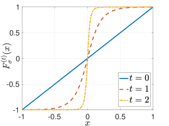
Figure 2: $F_{\sigma}^{(t)}(x)$ versus $x$ for different $t$ when $\sigma=0.5$.

4.3 Main Theorem

By applying the result in Theorem 2.B, the following theorem provides an exact characterization for the generalization error at each iteration $t$ for $m$ large enough.

Theorem 3 (Exact gen-error for iterative SSL under bGMM).

Fix any $\sigma\in\mathbb{R}_{+}$, $d\in\mathbb{N}$. The gen-error at $t=0$ is given by

$$\mathrm{gen}_{0}(P_{\mathbf{Z}},P_{\mathbf{X}},P_{\bm{\theta}_{0}|S_{\mathrm{l}},S_{\mathrm{u}}})=\frac{d}{n}.$$ (22)

Let $\alpha=\alpha(\xi_{0},\bm{\mu}^{\bot})$. For each $t\in[1:\tau]$, for almost all sample paths (i.e., almost surely),

$$\mathrm{gen}_{t}(P_{\mathbf{Z}},P_{\mathbf{X}},\{P_{\bm{\theta}_{k}|S_{\mathrm{l}},S_{\mathrm{u}}}\}_{k=0}^{t},\{f_{\bm{\theta}_{k}}\}_{k=0}^{t-1})$$

$$=\mathbb{E}_{\xi_{0},\bm{\mu}^{\bot}}\bigg{[}\frac{(m-1)(J_{\sigma}^{2}(F_{\sigma}^{(t-1)}(\alpha))+K_{\sigma}^{2}(F_{\sigma}^{(t-1)}(\alpha)))}{m\sigma^{2}}-\frac{J_{\sigma}(F_{\sigma}^{(t-1)}(\alpha))}{\sigma^{2}}\bigg{]}+o(1),$$ (23)

where $o(1)$ is a term that vanishes as $m\to\infty$.

The proof of Theorem 3 is provided in Appendix C. Several remarks are in order.

First, the gen-error at $t=0$ corresponds to the asymptotic result of supervised maximum likelihood estimation in works by Akaho and Kappen (2000) and Aminian et al. (2021). We numerically plot the quantity in (23), $g_{\sigma}^{(m)}(x):=((m-1)(J_{\sigma}^{2}(x)+K_{\sigma}^{2}(x))-mJ_{\sigma}(x))/\sigma^{2}$, for $x\in[-1,1]$ in Figure 12 in Appendix C, which shows that for all $\sigma_{1}>\sigma_{2}$, $g_{\sigma_{1}}^{(m)}(x)>g_{\sigma_{2}}^{(m)}(x)$ when $x>0$. From (17), we can see that $\alpha$ is close to 1 of high probability, which means that $\sigma\mapsto g_{\sigma}(x)$ is monotonically increasing in $\sigma$ with high probability. As a result, (23) increases as $\sigma$ increases. This is consistent with the intuition that when the training data have larger overlap between classes, it is more difficult to generalize well. Moreover, $F_{\sigma}^{(t)}(\alpha)$ is also close to 1 of high probability, and thus (23) saturates with $t$ quickly.

Second, by ignoring the $o(1)$ term, we compare the theoretical $\mathrm{gen}_{t}$ (cf. (22) and (23)) and the empirical gen-error from the repeated synthetic experiments with $d=2$, $n=10$ and $m=1000$, as shown in Figure 3. It can be seen that the theoretical $\mathrm{gen}_{t}$ matches the empirical gen-error well, which means that the characterization in (23) serves as a useful rule-of-thumb for how the gen-error changes over the SSL iterations. When the variance is small (e.g., $\sigma^{2}=0.6^{2}$), as shown in Figure 3(a), the gen-error decreases significantly from $t=0$ to $t=1$ and then quickly converges to a non-zero constant. Recall the correlation evolution function $F_{\sigma}$ in (19). Given any pair of $(\xi_{0},\bm{\mu}^{\bot})$, if $\alpha(\xi_{0},\bm{\mu}^{\bot})>0$, $F_{\sigma}^{(t)}(\alpha(\xi_{0},\bm{\mu}^{\bot}))>F_{\sigma}^{(t-1)}(\alpha(\xi_{0},\bm{\mu}^{\bot}))$ for all $t\in[1:\tau]$, as shown in Figure 2. This means that if the quality of the labelled data $S_{\mathrm{l}}$ is reasonably good, by using $\bm{\theta}_{0}$ which is learned from $S_{\mathrm{l}}$, the generated pseudo-labels for the unlabelled data are largely correct. Then the subsequent parameters $\bm{\theta}_{t}$ for $t\geq 1$ learned from the large number of pseudo-labelled data examples can improve the generalization error. With sufficiently large amount of training data, algorithm converges at very early stage. In addition, for more general cases (e.g., non-diagonal class covariance matrices), it takes more iterations for the gen-error to reach a plateau, as shown in Figure 5.

When the variance is large (e.g. $\sigma^{2}=3^{2}$), as shown in Figure 3(b), the gen-error increases with iteration $t$. The result shows that when the overlap between different classes is large enough, using the unlabelled data may not be able to improve the generalization performance. The intuition is that at the initial iteration with a limited number of labelled data, the learned parameter $\bm{\theta}_{0}$ cannot pseudo-label the unlabelled data with sufficiently high accuracy. Thus, the unlabelled data is not labelled well by the pseudo-labelling operation and hence, cannot help to improve the generalization error. To gain more insight, in Figure 5, we numerically plot $\mathrm{gen}_{1}$ versus different values of $\sigma$ under the same setting. It is interesting to find that there exists a $\sigma_{0}$ such that for $\sigma<\sigma_{0}$, $\mathrm{gen}_{1}<\mathrm{gen}_{0}$, which means the gen-error can be reduced with the help of abundant unlabelled data, while for $\sigma>\sigma_{0}$, using the unlabelled data can even harm the generalization performance.

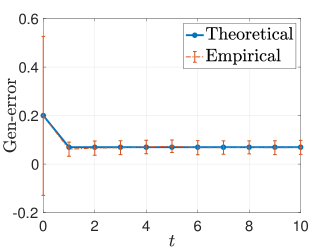
(a) $\sigma=0.6$

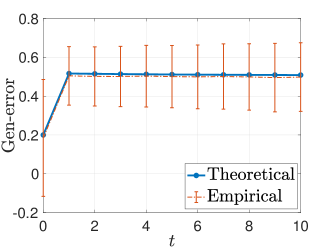
(b) $\sigma=3$

Figure 3: Comparison of the theoretical $\mathrm{gen}_{t}$ and the empirical gen-error at each iteration $t$.

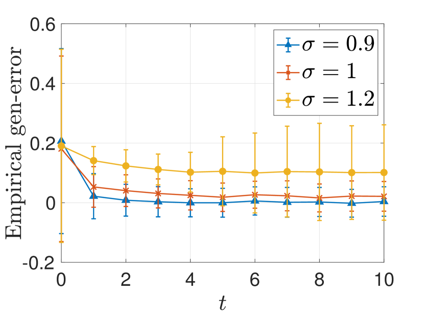
Figure 4: Empirical gen-error with covariance matrix $\sigma^{2}\times[0.6,0.3;0.3,0.8]$.

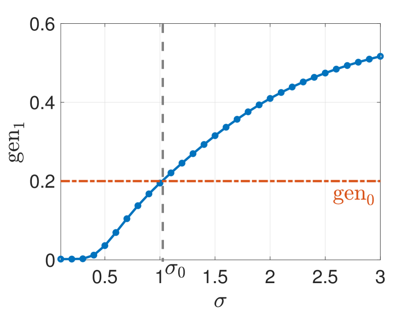
Figure 5: Theoretical gen-error at $t\!=\!1$ versus different std. devs. $\sigma\in[0.1,3]$.

Third, let us examine the effect of $n$, the number of labelled training samples. By expanding $\alpha$, defined in (17), using a Taylor series, we have

$$\alpha=1-\frac{\sigma^{2}}{2n}\|\bm{\mu}^{\bot}\|_{2}^{2}+o\bigg{(}\frac{1}{n}\bigg{)}.$$ (24)

It can be seen that as $n$ increases, $\alpha$ converges to $1$ in probability. Suppose the dimension $d=2$ and $\bm{\mu}=(1,0)$. Then $\bm{\mu}^{\bot}=[0,\mu_{2}^{\bot}]$ where $\mu_{2}^{\bot}\sim\mathcal{N}(0,1)$. By letting $m\to\infty$, the gen-error $\mathrm{gen}_{1}$ (cf. (23)) can be rewritten as

$$\mathrm{gen}_{1}\approx\int_{-\sqrt{2}}^{\sqrt{2}}\sqrt{\frac{n}{\pi\sigma^{2}}}\,e^{-\frac{ny^{2}}{\sigma^{2}}}\,g_{\sigma}^{\infty}(1-y^{2})~{}\mathrm{d}y,$$ (25)

where $g_{\sigma}^{(\infty)}(1-y^{2}):=(J_{\sigma}^{2}(1-y^{2})+K_{\sigma}^{2}(1-y^{2})-J_{\sigma}(1-y^{2}))/\sigma^{2}$ and thus, $\mathrm{gen}_{1}$ is a decreasing function of $n$. We further deduce that for any $t$, $\mathrm{gen}_{t}$ is decreasing in $n$.

Fourth, we consider an “enhanced” scenario in which the labelled data in $S_{\mathrm{l}}$ are reused in each iteration. Set $w=\frac{n}{n+m}$ in (4). We can extend Theorem 3 to Corollary 10 provided in Appendix F. It can be seen from Figure 17 that $\mathrm{gen}_{t}$ still decreases from $t=0$ to $1$ and saturates afterwards. We find that when $\sigma=0.6$, $n=10$, $m=1000$, the gen-error is almost the same as that one in Figure 3(a), which means that for large enough $\frac{m}{n}$, reusing the labelled data does not necessarily help to improve the generalization performance. Moreover, when $m=100$, $\mathrm{gen}_{t}$ is higher than that for $m=1000$, which coincides with the intuition that increasing the number of unlabelled data helps to reduce the generalization error.

Fifth, it is natural to wonder what the effect is when $m$, the number of unlabelled data examples, is held fixed and $n$, the number of labelled data examples, increases. In Figure 6, we numerically plot $\mathrm{gen}_{0}=\frac{d}{n}$ in (22) and (the theoretical) $\mathrm{gen}_{1}$ in (23) for $n$ ranging from $2$ to $50$, $m=1000$, $\sigma=0.6$ and $d=2$. As $n$ increases, $\mathrm{gen}_{0}$ and $\mathrm{gen}_{1}$ both decrease, which is as expected. However, when $n$ is larger than a certain value ($30$ in this case), we find that $\mathrm{gen}_{0}$ becomes smaller than $\mathrm{gen}_{1}$. This implies that with sufficiently many labelled training data, the generalization error based on the labelled training data is already sufficiently low, and incorporating the pseudo-labelled data in fact adversely affects the generalization error. Understanding this phenomenon precisely is an interesting avenue for future work.

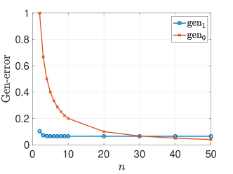
Figure 6: $\mathrm{gen}_{0}$ vs. $\mathrm{gen}_{1}$ for different $n$.

Finally, to verify the validity of the gen-error upper bound in Theorem 2.A, we further apply the bound to this setup and prove that the upper bound exhibits similar behaviour of the evolution of gen-error as $t$ increases. See Appendix D.

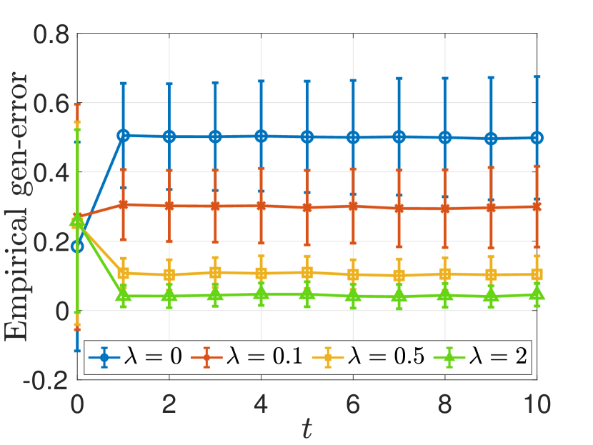
Figure 7: Empirical gen-error versus $t$ for $\sigma=3$ for different $\lambda$.

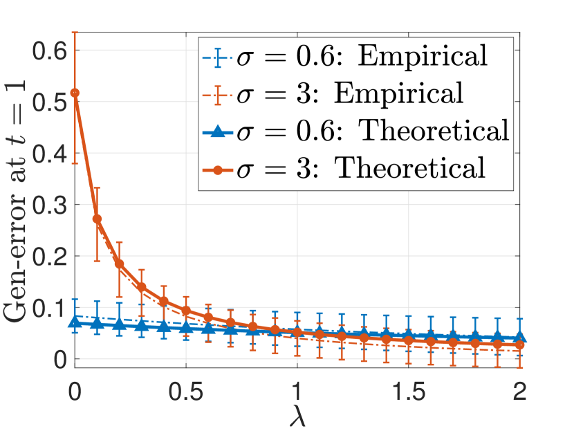
Figure 8: Theoretical and empirical $\mathrm{gen}_{1}$ vs.  $\lambda$ for different $\sigma$.

5 Improving the Gen-Error for Difficult Problems via Regularization

In Section 4.3, it is shown that for difficult classification problems with large class conditional variance, the gen-error increases after using pseudo-labelled data. The reason is that the learned initial parameter $\bm{\theta}_{0}$ can only generate low-accurate pseudo-labels and thus the pseudo-labelled data cannot help improve the generalization performance. In this section, we prove that by adding regularization to the loss function, we can mitigate the undesirable increase of gen-error across the pseudo-labelling iterations.

Since $\mathrm{gen}_{0}$ in (22) does not depend on data variance $\sigma^{2}$, here we focus on subsequent iterations $t\in[1:\tau]$. By considering the $\ell_{2}$ regularization (i.e., adding $\frac{\lambda}{2}\|\bm{\theta}\|_{2}^{2}$ to (15)), we obtain the new parameters (cf. (16)) as follows

$$\bm{\theta}_{t}^{\mathrm{reg}}=\frac{\bm{\theta}_{t}}{1+\sigma^{2}\lambda},\quad\forall\,t\in[1:\tau].$$ (26)

The derivations are provided in Appendix H. By applying Theorem 3, the following theorem provides a characterization for the gen-error of the case with regularization at each iteration $t$ for $m$ large enough. Let $\mathrm{gen}_{t}^{\mathrm{reg}}$ denotes the gen-error of the case with regularization and we drop the fixed quantities $(P_{\mathbf{Z}},P_{\mathbf{X}},\{P_{\bm{\theta}_{k}|S_{\mathrm{l}},S_{\mathrm{u}}}\}_{k=0}^{t},\{f_{\bm{\theta}_{k}}\}_{k=0}^{t-1})$ for notational simplicity.

Theorem 4 (Gen-error with regularization).

Fix any $d\in\mathbb{N}$, and $\sigma,\lambda\in\mathbb{R}_{+}$. The gen-error at any $t\in[1:\tau]$ is

$$\mathrm{gen}_{t}^{\mathrm{reg}}=\frac{\mathrm{gen}_{t}}{1+\sigma^{2}\lambda}.$$ (27)

The proof of Theorem 4 is provided in Appendix H. From (27), we observe that as $\lambda$ increases, the gen-error decreases. In Figure 8, we first empirically show that regularization can help mitigate the increase of gen-error during SSL iterations for hard-to-distinguish classes by comparing the empirical gen-error under $\lambda=0,0.1,0.5,2$ when $\sigma=3$ and $d=2$. Then in Figure 8, we plot the theoretical gen-error in (27) versus $\lambda$ when $t=1$ for the cases with small and large variances, i.e., $\sigma^{2}=0.6^{2}$ and $\sigma^{2}=3^{2}$. We also compare the theoretical results with the empirical gen-errors, which turn out to corroborate the theoretical ones. For the case with smaller variance, the improvement on gen-error is barely visible as $\lambda$ increases. For the case with larger variance, the decrease of the gen-error is more pronounced, which implies that $\ell_{2}$-regularization can effectively mitigate the impact on the gen-error induced by large class overlapping and pseudo-labels with low accuracy.

The adept reader might naturally wonder why one would not set $\lambda\to\infty$ in (27), which results in the gen-error tending to zero, which presumably is a desirable phenomenon. However, ultimately, what we wish to control is the expected population risk, which, according to (7), is the sum of the expected empirical risk on the training data and the gen-error. Even if the gen-error is zero, the expected population risk might be large. Hence, as $\lambda$ increases, we see a tradeoff between the gen-error and the empirical risk.

Classes	RGB-mean $\ell_{2}$ distance	RGB-variance $\ell_{2}$ distance	Difficulty
horse-ship	0.0180	3.90e-05	Easy
automobile-truck	0.0038	7.06e-05	Moderate
cat-dog	0.0007	4.95e-05	Challenging

Table 1: The $\ell_{2}$ distances between the RGB-mean and RGB-variance of different pairs of classes from the CIFAR10 dataset.

Classes	horse $\to$ship	ship $\to$horse	automobile $\to$truck	truck $\to$automobile	cat $\to$dog	dog $\to$cat
Number	17	3	61	64	93	137
Difficulty	Easy		Moderate		Challenging

Table 2: Number of images misclassified out of 1000 (Liu and Mukhopadhyay, 2018).

6 Experiments on Benchmark Datasets

To further illustrate that our theory is indeed behind the empirical behaviour of the iterative self-training with pseudo-labelling, in this section, we conduct experiments on real-world benchmark datasets, which demonstrates that our theoretical results on the bGMM example can also reflect the training dynamics on more realistic real-world tasks. The code to reproduce all the experiments can be found at https://github.com/HerianHe/GenErrorSSL_2022.git.

Recall that in the bGMM example, a higher standard deviation $\sigma$ represents a higher in-class variance, larger class-overlap, and consequently higher difficulty in classification. By a whitening argument, this also holds for bGMMs with non-isotropic covariance matrices. In our experiments on real-world data, we use the difficulty level of classification to mimic different in-class variances of bGMM. We pick two easy-to-distinguish class pairs (“automobile” and “truck”, “horse” and “ship”) from the CIFAR-10 dataset (Krizhevsky, 2009) as an analogy to bGMM with small in-class variance, and one difficult-to-distinguish class pair (“cat” and “dog”) from the same dataset as an analogy to bGMM with large in-class variance. Furthermore, to extend the analogy to multi-class classification, we conduct experiments on the 10-class MNIST dataset to gain more intuition.

We train deep neural networks (DNNs) via an iterative self-learning strategy (under the same setting as Figure 1) to perform binary and multi-class classification. In the first iteration, we only use a few labelled data examples to initialize the DNN with a sufficient number of epochs. In the subsequent iterations, we first sample a subset of unlabelled data and generate pseudo-labels for them via the model trained from the previous iteration. Then we update the model for a small number of epochs with both the labelled and pseudo-labelled data.

Experimental settings: For binary classification, we collect pairs of classes of images, i.e., “automobile” and “truck”, “horse” and “ship”, and “cat” and “dog” from the CIFAR10 (Krizhevsky, 2009) dataset. In this dataset, each class has $5000$ images for training and $1000$ images for testing. For each selected pair of classes, we manually divide the $10000$ training images into two sets: the labelled training set with $500$ images and the unlabelled training set with $9500$ images. We train a convolutional neural network, ResNet-10 (He et al., 2016), and use stochastic gradient descent (SGD) optimizer to minimize the cross-entropy loss. In PyTorch, the cross-entropy loss is defined as the negative logarithm of the output softmax probability corresponding to the true class, which is analogous to the NLL of the data under the parameters of the neural network. For the task with $\ell_{2}$-regularization, we train the neural network by setting different weight decay parameters (equivalent to $\lambda\times$ learning rate). In each pseudo-labelling iteration, we sample $2500$ unlabelled images. The complete training procedure lasts for $50$ self-training iterations.

We further validate our theoretical contributions on a multi-class classification problem in which we train a ResNet-6 model with the cross-entropy loss to perform $10$-class handwritten digits classification on the MNIST (LeCun et al., 1998) dataset. We sample $51000$ images from the training set, which contains $6000$ images for each of the ten classes. We divide them into two sets, i.e., a labelled training set with $1000$ images and an unlabelled set with $50000$ images. The optimizer and training iterations follow those in the aforementioned binary classification tasks without regularization.

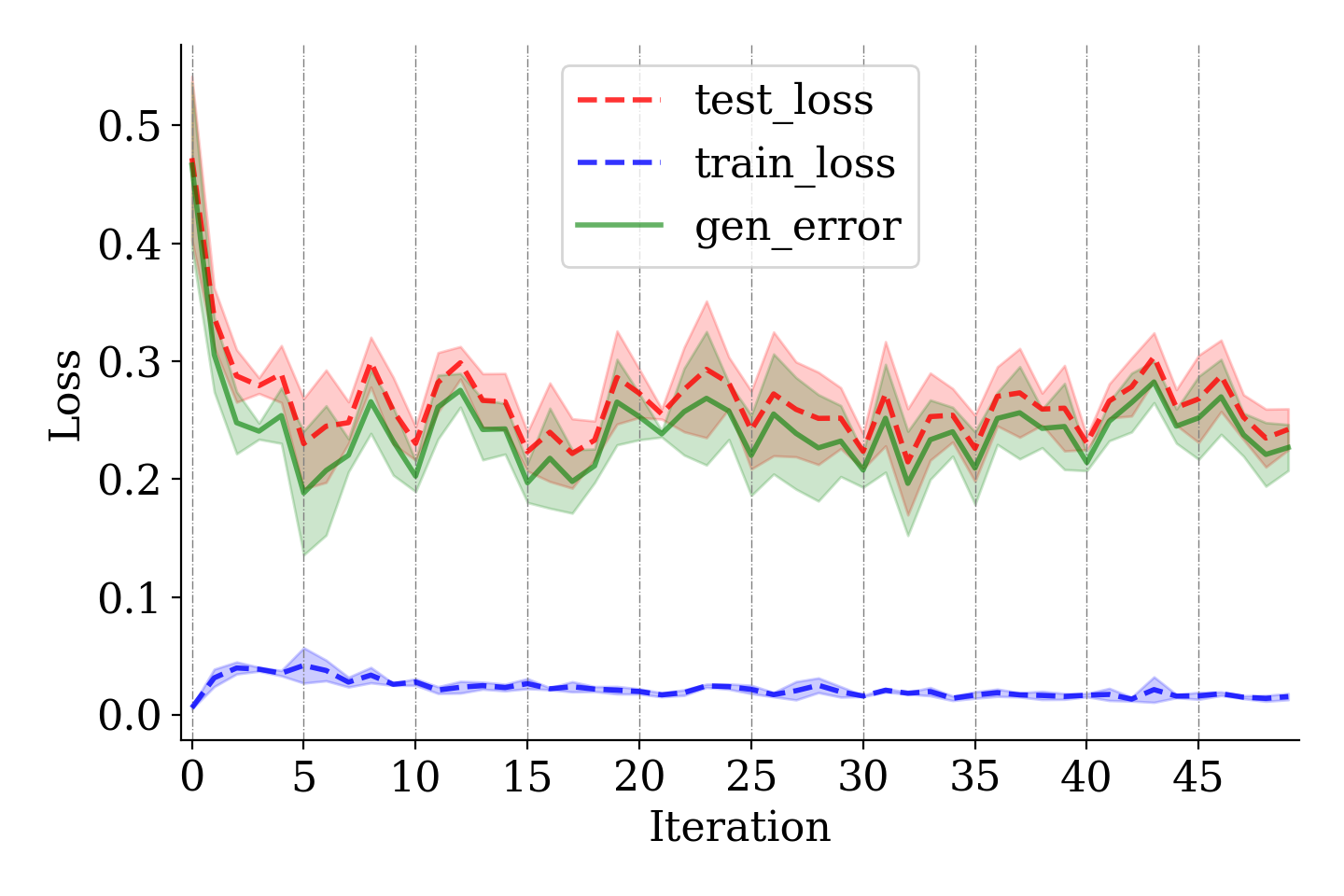
(a) “horse-ship”: gen-error

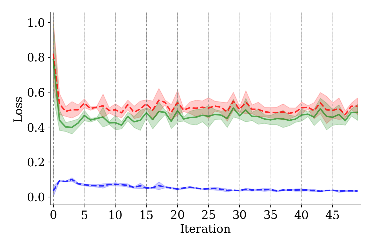
(b) “automobile-truck”: gen-error

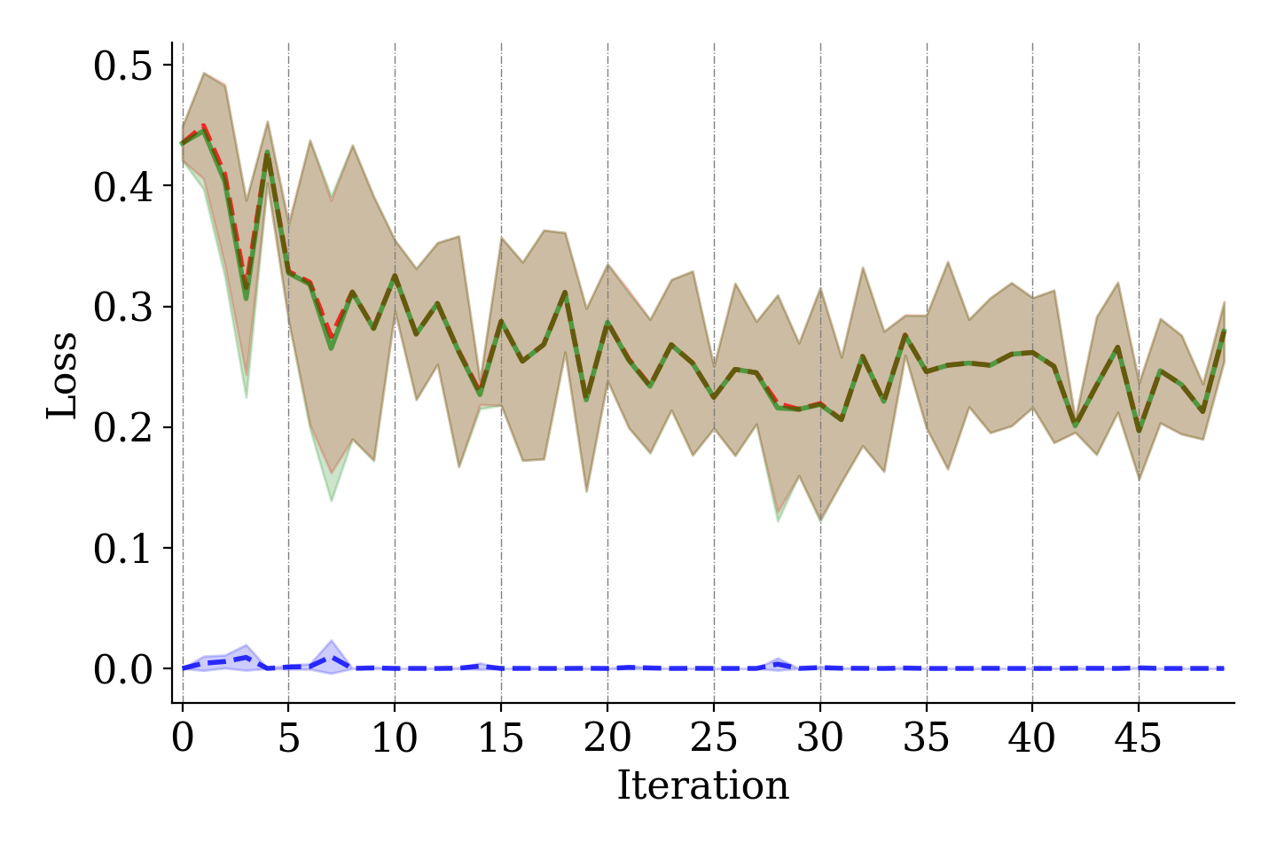
(c) MNIST: gen-error

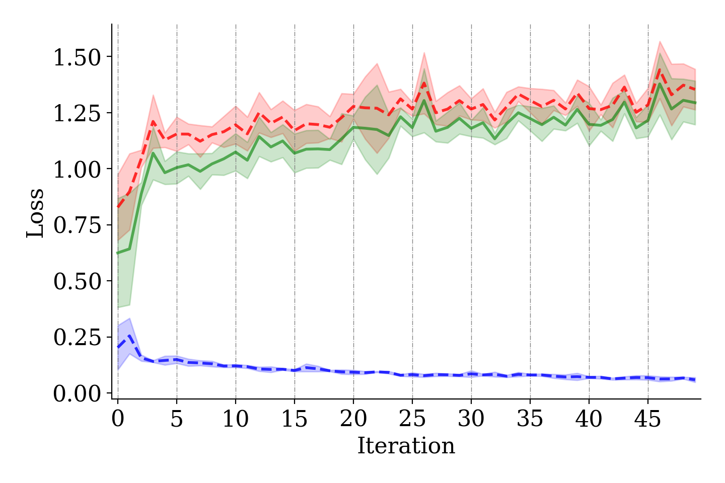
(d) “cat-dog”: gen-error

Figure 9: (a)–(c) & (e)–(g): easier-to-distinguish classes “horse” vs. “ship” and “automobile” vs. “truck”; (d),(h), (i)–(k): harder-to-distinguish classes “cat” vs. “dog”.

      

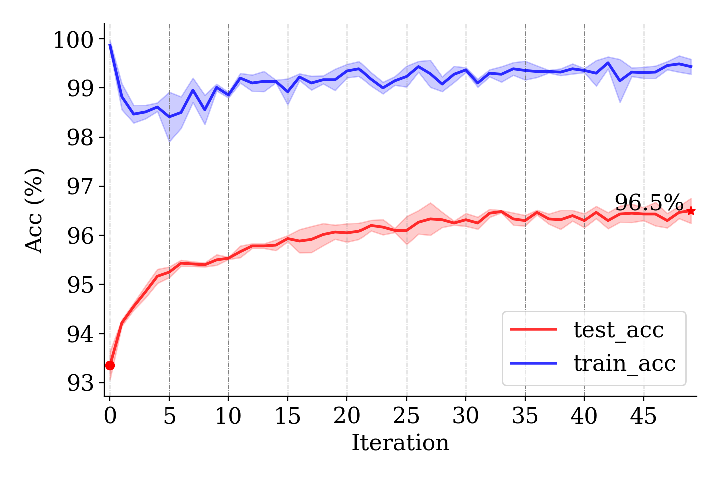
(e) “horse-ship”: accuracy

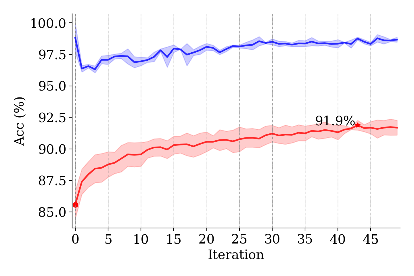
(f) “automobile-truck”: accuracy

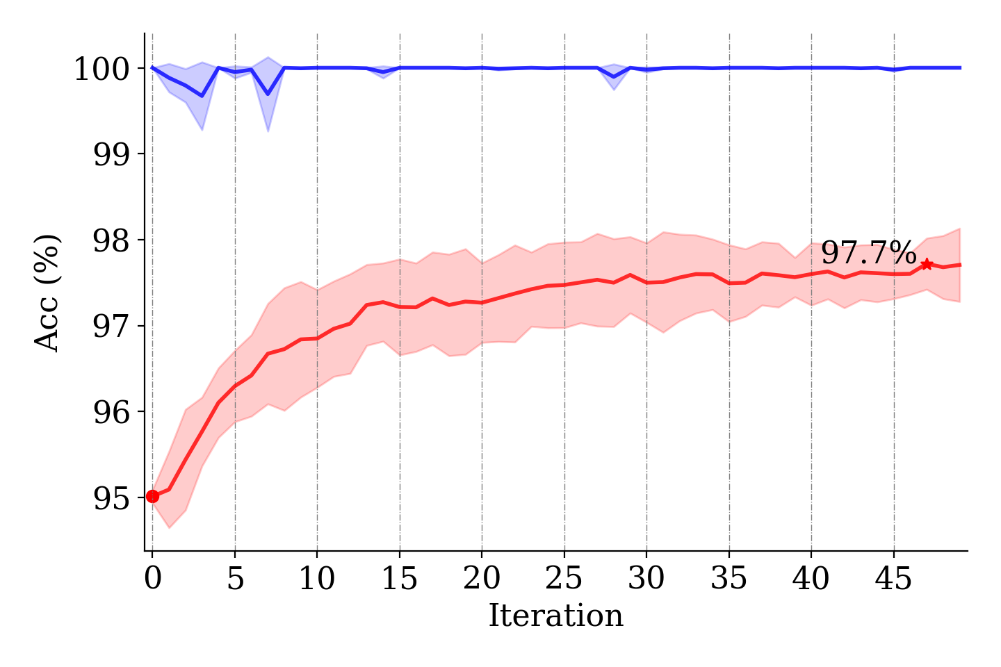
(g) MNIST: accuracy

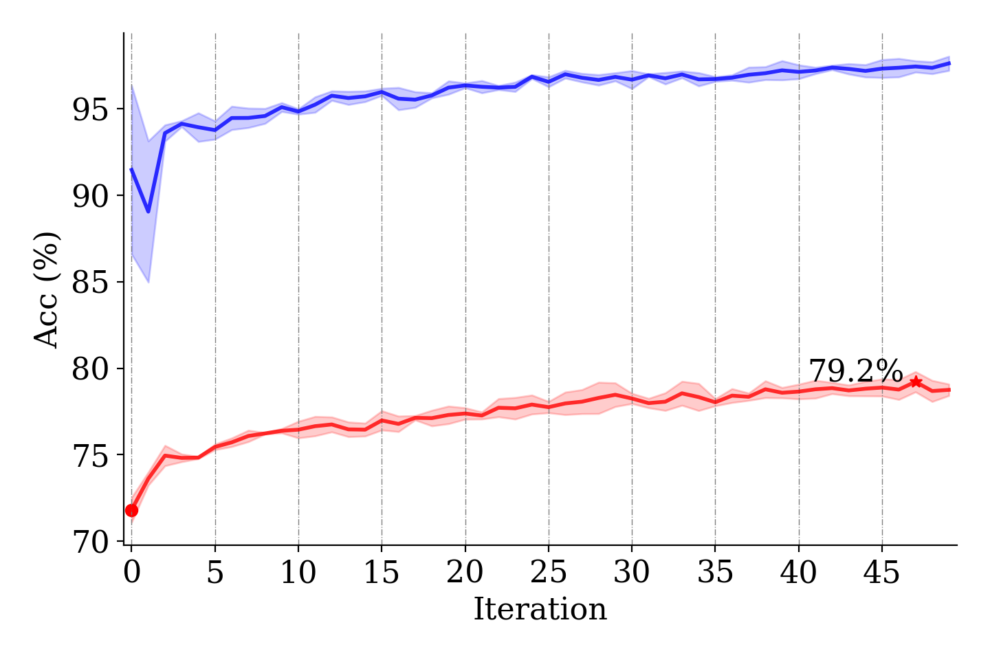
(h) “cat-dog”: accuracy

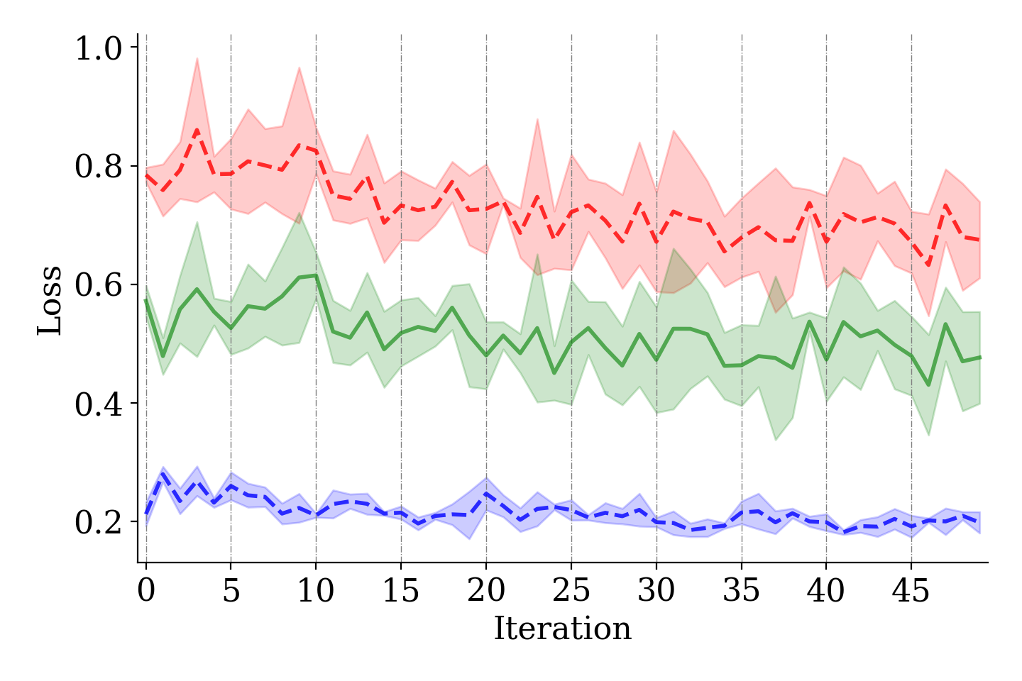
(i) “cat-dog”: gen-error with weight decay set to $5\times 10^{-4}$.

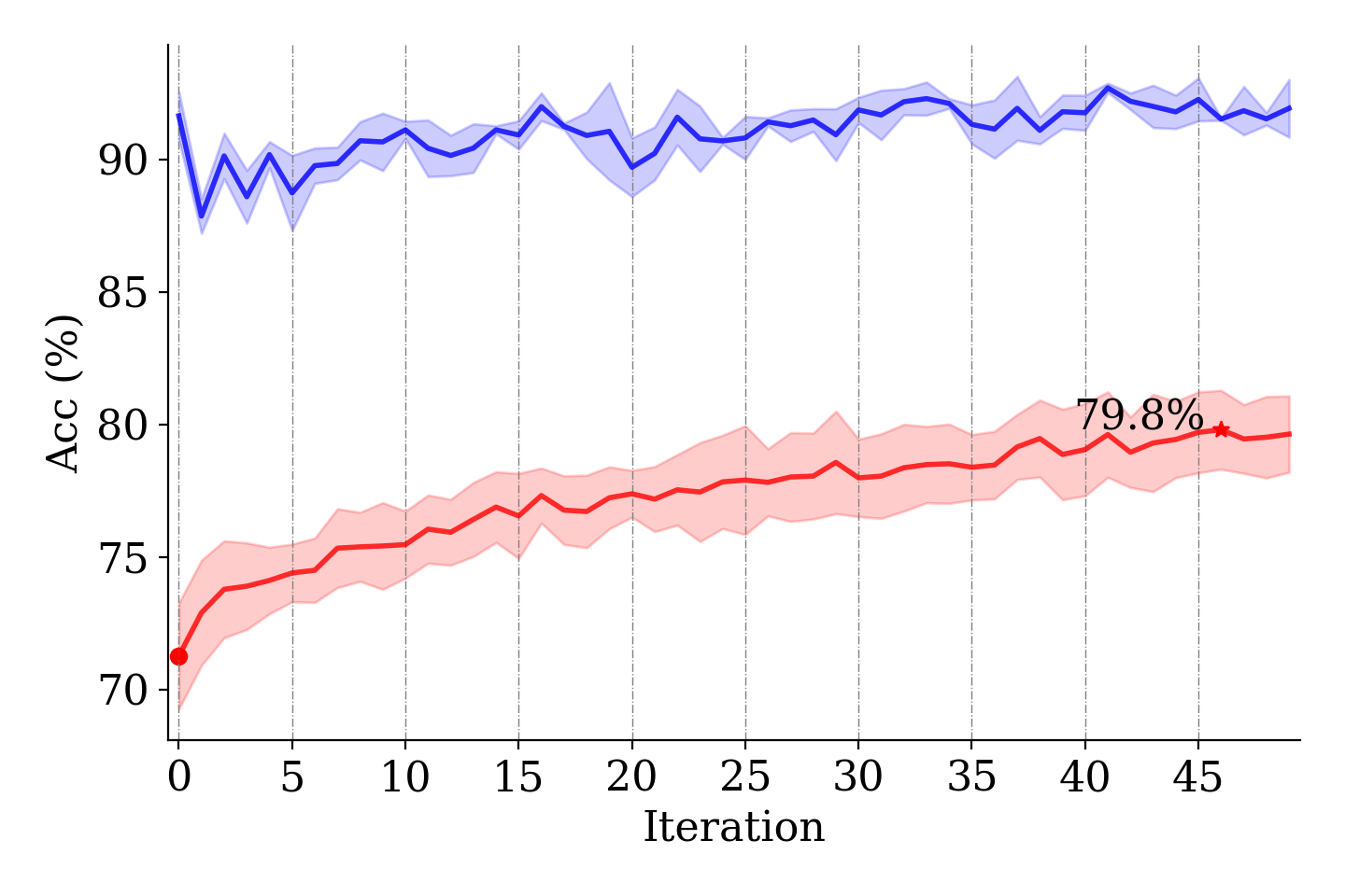
(j) “cat-dog”: accuracy with weight decay set to $5\times 10^{-4}$.

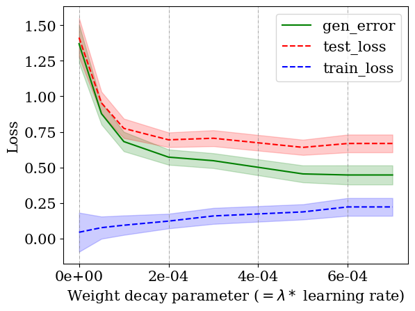
(k) “cat-dog”: gen-error after convergence versus weight decay.

Experimental observations: We perform each experiment $3$ times and report the average test and training (cross entropy) losses, the gen-error, and test and training accuracies in Figures 9(d). To illustrate the difficulty level of classification for each pair, we first calculated the mean and variance of the RGB (i.e., the red-green-blue color values) values of the images to show the difference of the images between the two classes. In Table 2, we display the RGB means and variances of the test data in six classes taken from the CIFAR10 dataset. We observe that the RGB variances of each pair are almost $0$ (and small compared to the RGB-mean $\ell_{2}$ distances), and thus, the RGB-mean $\ell_{2}$ distance is indicative of the difficulty of the classification task. Indeed, a smaller RGB-mean $\ell_{2}$ distance implies a higher overlap of the two classes and consequently, greater difficulty in distinguishing them. Therefore, the “cat-dog” pair, which is more difficult to disambiguate compared to the “horse-ship” and “automobile-truck” pairs, is analogous to the bGMM with large variance (i.e. large overlap between the positive and negative classes). Furthermore, in Table 2, we quote the commonly-used confusion matrix for the CIFAR10 dataset in (Liu and Mukhopadhyay, 2018, Fig. 7), which quantifies how many out of 1000 images of each class are misclassified to any other class. It is obvious that fewer misclassified images indicates lower classification difficulty, which corresponds with Table 2. These two tables provide an indication of the level of difficulty to distinguish different pairs of classes.

In Figures 9(a)–9(c), for easier-to-distinguish classes (based on the high classification accuracy and low loss, as well as Tables 2 and 2), the gen-error appears to have relatively large reduction in the early training iterations and then fluctuates around a constant value afterwards. For example, in Figure 9(a), the gen-error converges to around $0.25$ after $5$ iterations; in Figure 9(b), it converges to around $0.45$ after $5$ iterations. For multi-classification of MNIST in Figure 9(c), the gen-error also converges to around $0.25$ after $20$ iterations. These results corroborate the theoretical and empirical analyses in the bGMM case with small variance, which again verifies that Theorem 3 and Corollary 10 can shed light on the empirical gen-error on benchmark datasets. It also reveals that the generalization performance of iterative self-training on real datasets from relatively distinguishable classes can be quickly improved with the help of unlabelled data. In Figures 9(e), 9(f) and 9(g), we also show that the test accuracy increases with the iterations and has significant improvement compared to the initial iteration when only labelled data are used.

In Figures 9(d) and 9(h), we perform another binary classification experiment on the harder-to-distinguish pair, “cat” and “dog” (based on low accuracy at the initial point as well as Tables 2 and 2). We observe that the gen-error (and the test loss) does not decrease across the self-training iterations even though the test accuracy increases. This again corroborates the result in Figure 3(b) for the bGMM with large variance. The fact that both the test loss and test accuracy appear to increase with the iteration is, in fact, not contradictory. To intuitively explain this, in binary classification using the softmax (hence, logistic) function to predict the output classes, suppose the learned probability of a data example belonging to its true class is $p\in(1/2,1]$, the classification is correct. In other words, the accuracy is 100%. However, when $p$ (i.e., the classification confidence) decreases towards $(1/2)^{+}$, the corresponding decision margin $2p-1$ (Cao et al., 2019) also decreases and the test loss $-\log p$ increases commensurately. Thus, when the decision margin is small, even though the test accuracy may increase as the iteration counter increases, the test loss may also increase at the same time; this represents our lack of confidence.

We further investigate the effect of $\ell_{2}$-regularization on “cat-dog” classification. In Figures 9(i) and 9(j), we show that by setting the weight decay parameter to be $0.0005$, the increase of gen-error for the “cat-dog” classification task can be mitigated and the test accuracy is improved by 0.6% as well; compare this to Figures 9(d) and 9(h). In Figure 9(k), we plot the average gen-error over the last 10 iterations versus the weight decay parameter; this is shown to decrease as the weight decay increases (compared to Figure 8). In summary, our above observations correspond to that for the bGMM, namely that the unlabelled data do not always help to improve the gen-error but adding regularization can help to compensate for the undesirable impact.

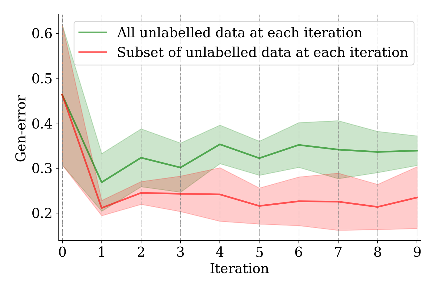
Figure 10: Comparison of the gen-error for the “horse” and “ship” classification task

Furthermore, we study the effect of reusing all the unlabelled data at each iteration. Under the same experimental setup as above, we conduct an additional experiment on the “horse-ship” pair in the CIFAR-10 dataset by using all $9,500$ unlabelled images in each iteration. The self-training procedure lasts for $10$ iterations. Figure 10 compares the gen-error of this additional experiment with the one of the same experiment in Figure 9(a). We find that when using the unlabelled data all at once, as the pseudo-labelling iteration increases, the gen-error is even higher than that for our original setup. This can possibly be attributed to overfitting.

7 Concluding Remarks and Future Work

In this paper, we have analyzed the gen-error of iterative SSL algorithms that pseudo-label large amounts of unlabelled data to progressively refine the parameters of a given model. We particularized the general bounds and exact expressions on the gen-error for the bGMM to gain some theoretical insight into the problem. These were then corroborated by experiments on benchmark datasets. The theoretical analyses and experimental results reinforce the main message of this paper—namely, that in the low-class-overlap or easy-to-classify scenario, pseudo-labelling can help to reduce the gen-error. On the other hand, for the high-class-overlap or difficult-to-classify scenario, pseudo-labelling can in fact hurt. Thus, the key takeaway from our paper is that practitioners should be judicious in adopting pseudo-labelling techniques, for they may degrade the overall performance.

There are three avenues for future research. First, our analytical results are only applicable to the bGMM. This yields valuable insights, but the model is admittedly restrictive. Generalizing our analyses to other statistical models for classification such as logistic regression will be instructive. Secondly, our work focuses on the gen-error. Often bounds on the population risk are desired as the population risk is the key determinant of the performance of classification algorithms. Bounding the population risk in the SSL setting would thus be interesting. Finally, analyzing other families of SSL algorithms beyond those that utilize pseudo-labelling would provide a clearer theoretical picture about the utility of SSL.

Acknowledgements

We sincerely thank the reviewers and action editor for their meticulous reading and insightful comments that led to a significantly improved version of the paper.

This research/project is supported by the National Research Foundation Singapore and DSO National Laboratories under the AI Singapore Programme (AISG Award No: AISG2-RP-2020-018), by an NRF Fellowship (A-0005077-01-00), and by Singapore Ministry of Education (MOE) AcRF Tier 1 Grants (A-0009042-01-00 and A-8000189-01-00).

Appendices

Appendix A Proof of Theorem 2.A

We commence with some notation. For any convex function $\psi:[0,b)\mapsto\mathbb{R}$, its Legendre dual $\psi^{*}$ is defined as $\psi^{*}(x):=\sup_{\lambda\in[0,b)}\lambda x-\psi(\lambda)$ for all $x\in[0,\infty)$. According to Boucheron et al. (2013, Lemma 2.4), when $\psi(0)=\psi^{\prime}(0)=0$, $\psi^{*}(x)$ is a nonnegative convex and nondecreasing function on $[0,\infty)$. Moreover, for every $y\geq 0$, its generalized inverse function $\psi^{*-1}(y):=\inf\{x\geq 0:\psi^{*}(x)\geq y\}$ is concave and can be rewritten as $\psi^{*-1}(y)=\inf_{\lambda\in[0,b)}\frac{y+\psi(\lambda)}{\lambda}$.

We first introduce the following theorem that is applicable to more general loss functions.

Theorem 5.

For any $\tilde{\theta}_{t}\in\Theta$, let $\psi_{-}(\lambda,\tilde{\theta}_{t})$ and $\psi_{+}(\lambda,\tilde{\theta}_{t})$ be convex functions of $\lambda$ and $\psi_{+}(0,\tilde{\theta}_{t})=\psi_{+}^{\prime}(0,\tilde{\theta}_{t})=\psi_{-}(0,\tilde{\theta}_{t})=\psi_{-}^{\prime}(0,\tilde{\theta}_{t})=0$. Assume that $\Lambda_{l(\tilde{\theta}_{t},\tilde{Z})}(\lambda,\tilde{\theta}_{t})\leq\psi_{+}(\lambda,\tilde{\theta}_{t})$ for all $\lambda\in[0,b_{+})$ and $\Lambda_{l(\tilde{\theta}_{t},\tilde{Z})}(\lambda,\tilde{\theta}_{t})\leq\psi_{-}(\lambda,\tilde{\theta}_{t})$ for $\lambda\in(b_{-},0]$ under distribution $P_{\tilde{Z}|\theta^{(t-1)}}=P_{Z}$, where $0<b_{+}\leq\infty$ and $-\infty\leq b_{-}<0$. Let $\psi_{+}(\lambda)=\sup_{\tilde{\theta}_{t}}\psi_{+}(\lambda,\tilde{\theta}_{t})$ and $\psi_{-}(\lambda)=\sup_{\tilde{\theta}_{t}}\psi_{-}(\lambda,\tilde{\theta}_{t})$. We have

$$\mathrm{gen}_{t}(P_{Z},P_{X},\{P_{\theta_{k}|S_{\mathrm{l}},S_{\mathrm{u}}}\}_{k=0}^{t},\{f_{\theta_{k}}\}_{k=0}^{t-1})$$

$$\leq\frac{w}{n}\sum_{i=1}^{n}\mathbb{E}_{\theta^{(t-1)}}\left[\psi_{-}^{*-1}(I_{\theta^{(t-1)}}(\theta_{t};Z_{i}))\right]$$

$$\quad+\frac{1-w}{m}\sum_{i\in\mathcal{I}_{t}}\mathbb{E}_{\theta^{(t-1)}}\left[\psi_{-}^{*-1}\big{(}I_{\theta^{(t-1)}}(\theta_{t};X_{i}^{\prime},\hat{Y}_{i}^{\prime})+D_{\theta^{(t-1)}}(P_{X_{i}^{\prime},\hat{Y}_{i}^{\prime}}\|P_{Z})\big{)}\right],$$ (28)

and

$$-\mathrm{gen}_{t}(P_{Z},P_{X},\{P_{\theta_{k}|S_{\mathrm{l}},S_{\mathrm{u}}}\}_{k=0}^{t},\{f_{\theta_{k}}\}_{k=0}^{t-1})$$

$$\leq\frac{w}{n}\sum_{i=1}^{n}\mathbb{E}_{\theta^{(t-1)}}\left[\psi_{+}^{*-1}(I_{\theta^{(t-1)}}(\theta_{t};Z_{i}))\right]$$

$$\quad+\frac{1-w}{m}\sum_{i\in\mathcal{I}_{t}}\mathbb{E}_{\theta^{(t-1)}}\left[\psi_{+}^{*-1}\big{(}I_{\theta^{(t-1)}}(\theta_{t};X_{i}^{\prime},\hat{Y}_{i}^{\prime})+D_{\theta^{(t-1)}}(P_{X_{i}^{\prime},\hat{Y}_{i}^{\prime}}\|P_{Z})\big{)}\right],$$ (29)

where $P_{X_{i}^{\prime},\hat{Y}_{i}^{\prime}|\theta^{(t-1)}}(x,y|\hat{\theta}^{(t-1)})=P_{X}(x)\text{1}\{y=f_{\hat{\theta}_{t-1}}(x)\}$ for any $x\in\mathcal{X}$, $y\in\mathcal{Y}$ and $\hat{\theta}^{(t-1)}\in\Theta^{t-1}$, and $P_{Z|\theta^{(t-1)}}=P_{Z}$.

Proof  Consider the Donsker–Varadhan variational representation of the KL-divergence between any two distributions $P$ and $Q$ on $\mathcal{X}$:

$$D(P\|Q)=\sup_{g\in\mathcal{G}}\Big{\{}\mathbb{E}_{X\sim P}[g(X)]-\log\mathbb{E}_{X\sim Q}[e^{g(X)}]\Big{\}},$$ (30)

where the supremum is taken over the set of measurable functions in $\mathcal{G}=\{g:\mathcal{X}\mapsto\mathbb{R}:\mathbb{E}_{X\sim Q}[e^{g(X)}]<\infty\}$.

Recall that $\tilde{\theta}_{t}$ and $\tilde{Z}$ are independent copies of $\theta_{t}$ and $Z$ respectively, such that $P_{\tilde{\theta}_{t},\tilde{Z}}=Q_{\theta_{t}}\otimes P_{Z}$, $P_{\tilde{\theta}_{t},\tilde{Z}|\theta^{(t-1)}}=P_{\theta_{t}|\theta^{(t-1)}}\otimes P_{Z}$. For any iterative SSL algorithm, by applying the law of total expectation, the generalization error can be rewritten as

$$\mathrm{gen}_{t}(P_{Z},P_{X},\{P_{\theta_{k}|S_{\mathrm{l}},S_{\mathrm{u}}}\}_{k=0}^{t},\{f_{\theta_{k}}\}_{k=0}^{t-1})$$

$$=w\bigg{(}\mathbb{E}_{\theta_{t}}[\mathbb{E}_{Z}[l(\theta_{t},Z)]]-\frac{1}{n}\sum_{i=1}^{n}\mathbb{E}_{\theta_{t},Z_{i}}[l(\theta_{t},Z_{i})]\bigg{)}$$

$$\quad+(1-w)\bigg{(}\mathbb{E}_{\theta_{t}}[\mathbb{E}_{Z}[l(\theta_{t},Z)]]-\frac{1}{m}\sum_{i\in\mathcal{I}_{t}}\mathbb{E}_{\theta_{t},X^{\prime}_{i},\hat{Y}^{\prime}_{i}}[l(\theta_{t},(X^{\prime}_{i},\hat{Y}^{\prime}_{i}))]\bigg{)}$$ (31)

$$=\frac{w}{n}\sum_{i=1}^{n}\bigg{(}\mathbb{E}_{\tilde{\theta}_{t},\tilde{Z}}[l(\tilde{\theta}_{t},\tilde{Z})]-\mathbb{E}_{\theta_{t},Z_{i}}[l(\theta_{t},Z_{i})]\bigg{)}$$

$$\quad+\frac{1-w}{m}\sum_{i\in\mathcal{I}_{t}}\bigg{(}\mathbb{E}_{\tilde{\theta}_{t},\tilde{Z}}[l(\tilde{\theta}_{t},\tilde{Z})]-\mathbb{E}_{\theta_{t},X^{\prime}_{i},\hat{Y}^{\prime}_{i}}[l(\theta_{t},(X^{\prime}_{i},\hat{Y}^{\prime}_{i}))]\bigg{)}$$ (32)

$$=\frac{w}{n}\sum_{i=1}^{n}\mathbb{E}_{\theta^{(t-1)}}\Big{[}\mathbb{E}_{\tilde{\theta}_{t},\tilde{Z}}\big{[}l(\tilde{\theta}_{t},\tilde{Z})|\theta^{(t-1)}\big{]}-\mathbb{E}_{\theta_{t},Z_{i}}\big{[}l(\theta_{t},Z_{i})|\theta^{(t-1)}\big{]}\Big{]}$$

$$\quad+\frac{1-w}{m}\sum_{i\in\mathcal{I}_{t}}\mathbb{E}_{\theta^{(t-1)}}\Big{[}\mathbb{E}_{\tilde{\theta}_{t},\tilde{Z}}\big{[}l(\tilde{\theta}_{t},\tilde{Z})|\theta^{(t-1)}\big{]}-\mathbb{E}_{\theta_{t},X^{\prime}_{i},\hat{Y}^{\prime}_{i}}\big{[}l(\theta_{t},(X^{\prime}_{i},\hat{Y}^{\prime}_{i}))|\theta^{(t-1)}\big{]}\Big{]}.$$ (33)

Note that $\psi_{+}(\lambda)=\sup_{\tilde{\theta}_{t}}\psi_{+}(\lambda,\tilde{\theta}_{t})$ and $\psi_{-}(\lambda)=\sup_{\tilde{\theta}_{t}}\psi_{-}(\lambda,\tilde{\theta}_{t})$ are convex, and so their Legendre duals $\psi_{-}^{*}$, $\psi_{+}^{*}$, and the corresponding inverses are well-defined.

Let $\check{l}(\theta,z)=l(\theta,z)-\mathbb{E}_{Z}[l(\theta,Z)]$. We have the fact that $\mathbb{E}_{\tilde{Z}}[\check{l}(\tilde{\theta}_{t},\tilde{Z})]=0$ for any $\tilde{\theta}_{t}$. Again, by the Donsker–Varadhan variational representation of the KL-divergence, for any fixed $\theta^{(t-1)}$ and any $\lambda\in[0,b_{+})$, we have

$$I_{\theta^{(t-1)}}(\theta_{t};Z)=D(P_{\theta_{t},Z|\theta^{(t-1)}}\|P_{\theta_{t}|\theta^{(t-1)}}\otimes P_{Z})$$

$$\geq\mathbb{E}_{\theta_{t},Z}[\lambda\check{l}(\theta_{t},Z)|\theta^{(t-1)}]-\log\mathbb{E}_{\tilde{\theta}_{t},\tilde{Z}}[e^{\lambda\check{l}(\tilde{\theta}_{t},\tilde{Z})}|\theta^{(t-1)}]$$ (34)

$$=\mathbb{E}_{\theta_{t},Z}[\lambda\check{l}(\theta_{t},Z)|\theta^{(t-1)}]-\log\mathbb{E}_{\tilde{\theta}_{t}|\theta^{(t-1)}}\mathbb{E}_{\tilde{Z}}\big{[}e^{\lambda\check{l}(\tilde{\theta}_{t},\tilde{Z})}\big{]}$$ (35)

$$=\mathbb{E}_{\theta_{t},Z}[\lambda\check{l}(\theta_{t},Z)|\theta^{(t-1)}]-\log\mathbb{E}_{\tilde{\theta}_{t}|\theta^{(t-1)}}\big{[}\exp\big{(}\Lambda_{l(\tilde{\theta}_{t},\tilde{Z})}(\lambda,\tilde{\theta}_{t})\big{)}\big{]}$$ (36)

$$\geq\lambda\mathbb{E}_{\theta_{t},Z}[l(\theta_{t},Z)-\mathbb{E}_{Z}[l(\theta_{t},Z)]|\theta^{(t-1)}]-\log\mathbb{E}_{\tilde{\theta}_{t}|\theta^{(t-1)}}\big{[}\exp(\psi_{+}(\lambda,\tilde{\theta}_{t}))\big{]}$$ (37)

$$\geq\lambda\mathbb{E}_{\theta_{t},Z}[l(\theta_{t},Z)-\mathbb{E}_{Z}[l(\theta_{t},Z)]|\theta^{(t-1)}]-\psi_{+}(\lambda)$$ (38)

$$=\lambda\big{(}\mathbb{E}_{\theta_{t},Z}[l(\theta_{t},Z)|\theta^{(t-1)}]-\mathbb{E}_{\tilde{\theta}_{t},\tilde{Z}}[l(\tilde{\theta}_{t},\tilde{Z})|\theta^{(t-1)}]\big{)}-\psi_{+}(\lambda).$$ (39)

where (36) follows from the definition of $\Lambda_{l(\tilde{\theta}_{t},\tilde{Z})}(\lambda,\tilde{\theta}_{t})$ in (49), (37) follows from the assumption that $\Lambda_{l(\tilde{\theta}_{t},\tilde{Z})}(\lambda,\tilde{\theta}_{t})\leq\psi_{+}(\lambda,\tilde{\theta}_{t})$ for all $\lambda\in[0,b_{+})$, and (38) follows because $\psi_{+}(\lambda)=\sup_{\tilde{\theta}_{t}}\psi_{+}(\lambda,\tilde{\theta}_{t})$. Thus, we have

$$\mathbb{E}_{\theta_{t},Z}[l(\theta_{t},Z)|\theta^{(t-1)}]-\mathbb{E}_{\tilde{\theta}_{t},\tilde{Z}}[l(\tilde{\theta}_{t},\tilde{Z})|\theta^{(t-1)}]$$

$$\leq\inf_{\lambda\in[0,b_{+})}\frac{I_{\theta^{(t-1)}}(\theta_{t};Z)+\psi_{+}(\lambda)}{\lambda}=\psi_{+}^{*-1}\big{(}I_{\theta^{(t-1)}}(\theta_{t};Z)\big{)}.$$ (40)

Similarly, for $\lambda\in(b_{-},0]$,

$$\mathbb{E}_{\tilde{\theta}_{t},\tilde{Z}}[l(\tilde{\theta}_{t},\tilde{Z})|\theta^{(t-1)}]-\mathbb{E}_{\theta_{t},Z}[l(\theta_{t},Z)|\theta^{(t-1)}]$$

$$\leq\inf_{\lambda\in[0,-b_{-})}\frac{I_{\theta^{(t-1)}}(\theta_{t};Z)+\psi_{-}(\lambda)}{\lambda}=\psi_{-}^{*-1}\big{(}I_{\theta^{(t-1)}}(\theta_{t};Z)\big{)}.$$ (41)

By applying the same techniques, for any pair of pseudo-labelled random variables $(X^{\prime},\hat{Y}^{\prime})$ used at iteration $t$ and any $\lambda\in[0,b_{+})$, we have

$$I_{\theta^{(t-1)}}(\theta_{t};X^{\prime},\hat{Y}^{\prime})+D_{\theta^{(t-1)}}(P_{X^{\prime},\hat{Y}^{\prime}}\|P_{Z})$$

$$=D_{\theta^{(t-1)}}(P_{\theta_{t},X^{\prime},\hat{Y}^{\prime}}\|P_{\theta_{t}}\otimes P_{X^{\prime},\hat{Y}^{\prime}})+D_{\theta^{(t-1)}}(P_{\theta_{t}}\otimes P_{X^{\prime},\hat{Y}^{\prime}}\|P_{\theta_{t}}\otimes P_{Z})$$ (42)

$$\geq\mathbb{E}_{\theta_{t},X^{\prime},\hat{Y}^{\prime}}[\lambda l(\theta_{t},(X^{\prime},\hat{Y}^{\prime}))|\theta^{(t-1)}]-\log\mathbb{E}_{\theta_{t}}\big{[}\mathbb{E}_{X^{\prime},\hat{Y}^{\prime}}[e^{\lambda l(\theta_{t},(X^{\prime},\hat{Y}^{\prime}))}|\theta^{(t-1)}]|\theta^{(t-1)}\big{]}$$

$$\quad+\mathbb{E}_{\theta_{t}}\big{[}\mathbb{E}_{X^{\prime},\hat{Y}^{\prime}}[\lambda l(\theta_{t},(X^{\prime},\hat{Y}^{\prime}))|\theta^{(t-1)}]|\theta^{(t-1)}\big{]}-\log\mathbb{E}_{\theta_{t}}\big{[}\mathbb{E}_{Z}[e^{\lambda l(\theta_{t},Z)}]|\theta^{(t-1)}\big{]}$$ (43)

$$\geq\mathbb{E}_{\theta_{t},X^{\prime},\hat{Y}^{\prime}}[\lambda l(\theta_{t},(X^{\prime},\hat{Y}^{\prime}))|\theta^{(t-1)}]-\log\mathbb{E}_{\theta_{t}}\big{[}\mathbb{E}_{Z}[e^{\lambda l(\theta_{t},Z)}]|\theta^{(t-1)}\big{]}$$ (44)

$$=\lambda\Big{(}\mathbb{E}_{\theta_{t},X^{\prime},\hat{Y}^{\prime}}[\lambda l(\theta_{t},(X^{\prime},\hat{Y}^{\prime}))|\theta^{(t-1)}]-\mathbb{E}_{\theta_{t}}\big{[}\mathbb{E}_{Z}[l(\theta_{t},Z)]|\theta^{(t-1)}\big{]}\Big{)}$$

$$\quad-\log\mathbb{E}_{\tilde{\theta}_{t}|\theta^{(t-1)}}\big{[}\exp\big{(}\Lambda_{l(\tilde{\theta}_{t},\tilde{Z})}(\lambda,\tilde{\theta}_{t})\big{)}\big{]}$$ (45)

$$\geq\lambda\Big{(}\mathbb{E}_{\theta_{t},X^{\prime},\hat{Y}^{\prime}}[\lambda l(\theta_{t},(X^{\prime},\hat{Y}^{\prime}))]-\mathbb{E}_{\theta_{t}}\big{[}\mathbb{E}_{Z}[l(\theta_{t},Z)]\big{]}\Big{)}-\psi_{+}(\lambda),$$ (46)

where (44) follows from Jensen’s inequality. Thus, we get

$$\mathbb{E}_{\theta_{t},X^{\prime}_{i},\hat{Y}^{\prime}_{i}}\big{[}l(\theta_{t},(X^{\prime},\hat{Y}^{\prime}))|\theta^{(t-1)}\big{]}-\mathbb{E}_{\tilde{\theta}_{t},\tilde{Z}}\big{[}l(\tilde{\theta}_{t},\tilde{Z})|\theta^{(t-1)}\big{]}$$

$$\leq\psi_{+}^{*-1}\big{(}I_{\theta^{(t-1)}}(\theta_{t};X^{\prime},\hat{Y}^{\prime})+D_{\theta^{(t-1)}}(P_{X^{\prime},\hat{Y}^{\prime}}\|P_{Z})\big{)}$$ (47)

and

$$\mathbb{E}_{\tilde{\theta}_{t},\tilde{Z}}\big{[}l(\tilde{\theta}_{t},\tilde{Z})|\theta^{(t-1)}\big{]}-\mathbb{E}_{\theta_{t},X^{\prime}_{i},\hat{Y}^{\prime}_{i}}\big{[}l(\theta_{t},(X^{\prime},\hat{Y}^{\prime}))|\theta^{(t-1)}\big{]}$$

$$\leq\psi_{-}^{*-1}\big{(}I_{\theta^{(t-1)}}(\theta_{t};X^{\prime},\hat{Y}^{\prime})+D_{\theta^{(t-1)}}(P_{X^{\prime},\hat{Y}^{\prime}}\|P_{Z})\big{)}.$$ (48)

The proof is completed by applying inequalities (40), (41), (47) and (48) to the expansion of $\mathrm{gen}_{t}$ in (33).  

Let $\tilde{\theta}_{t}$ and $\tilde{Z}$ be independent copies of $\theta_{t}$ and $Z$ respectively, such that $P_{\tilde{\theta}_{t},\tilde{Z}}=Q_{\theta_{t}}\otimes P_{Z}$, where $Q_{\theta_{t}}$ is the marginal distribution of $\theta_{t}$. For any fixed $\tilde{\theta}_{t}\in\Theta$, let the cumulant generating function (CGF) of $l(\tilde{\theta}_{t},\tilde{Z})$ be

$$\Lambda_{l(\tilde{\theta}_{t},\tilde{Z})}(\lambda,\tilde{\theta}_{t}):=\log\mathbb{E}_{\tilde{Z}}[e^{\lambda(l(\tilde{\theta}_{t},\tilde{Z})-\mathbb{E}_{\tilde{Z}}[l(\tilde{\theta}_{t},\tilde{Z})])}].$$ (49)

When the loss function $l(\theta,Z)\sim\mathrm{subG}(R)$ under $Z\sim P_{Z}$ for any $\theta\in\Theta$, we have $\Lambda_{l(\tilde{\theta}_{t},\tilde{Z})}(\lambda,\tilde{\theta}_{t})\leq\frac{R^{2}\lambda^{2}}{2}$ for all $\lambda\in\mathbb{R}$. Then we can let $\psi_{-}(\lambda,\tilde{\theta}_{t})=\psi_{+}(\lambda,\tilde{\theta}_{t})=\frac{R^{2}\lambda^{2}}{2}$ for all $\tilde{\theta}_{t}\in\Theta$. Hence, $\psi_{+}(\lambda)=\psi_{-}(\lambda)=\sup_{\tilde{\theta}_{t}\in\Theta}\frac{R^{2}\lambda^{2}}{2}=\frac{R^{2}\lambda^{2}}{2}$ and $\psi_{+}^{*-1}(y)=\psi_{-}^{*-1}(y)=\sqrt{2R^{2}y}$ for any $y\geq 0$. Finally, Theorem 2.A can then be directly obtained from Theorem 5.

Appendix B Proof of Theorem 2.B

Recall that $\tilde{\theta}_{t}$ and $\tilde{Z}$ are independent copies of $\theta_{t}$ and $Z$ respectively, such that $P_{\tilde{\theta}_{t},\tilde{Z}}=Q_{\theta_{t}}\otimes P_{Z}$, $P_{\tilde{\theta}_{t},\tilde{Z}|\theta^{(t-1)}}=P_{\theta_{t}|\theta^{(t-1)}}\otimes P_{Z}$.

Recall the gen-error given in (33). The first term in (33) can be rewritten as

$$\mathbb{E}_{\theta^{(t-1)}}\Big{[}\mathbb{E}_{\tilde{\theta}_{t},\tilde{Z}}\big{[}l(\tilde{\theta}_{t},\tilde{Z})|\theta^{(t-1)}\big{]}-\mathbb{E}_{\theta_{t},Z_{i}}\big{[}l(\theta_{t},Z_{i})|\theta^{(t-1)}\big{]}\Big{]}$$

$$=\mathbb{E}_{\tilde{\theta}_{t},\tilde{Z}}\big{[}-\log p_{\tilde{\theta}_{t}}\big{]}-\mathbb{E}_{\theta_{t},Z_{i}}\big{[}-\log p_{\theta_{t}}\big{]}$$ (50)

$$=\mathbb{E}_{\theta_{t}}\Big{[}h(P_{Z},p_{\theta_{t}})-h(P_{Z_{i}|\theta_{t}},p_{\theta_{t}})\Big{]}$$ (51)

$$=\mathbb{E}_{\theta_{t}}\Big{[}\mathrm{\Delta h}(P_{Z}\|P_{Z_{i}|\theta_{t}}|p_{\theta_{t}})\Big{]}.$$ (52)

The second term in (33) can be rewritten as

$$\mathbb{E}_{\tilde{\theta}_{t},\tilde{Z}}[l(\tilde{\theta}_{t},\tilde{Z})]-\mathbb{E}_{\theta_{t},X^{\prime}_{i},\hat{Y}^{\prime}_{i}}[l(\theta_{t},(X^{\prime}_{i},\hat{Y}^{\prime}_{i}))]$$

$$=\mathbb{E}_{\theta_{t},Z_{i}}[-\log p_{\theta_{t}}]-\mathbb{E}_{\theta_{t},X^{\prime}_{i},\hat{Y}^{\prime}_{i}}[-\log p_{\theta_{t}}]$$ (53)

$$=\mathbb{E}_{\theta^{(t-1)}}\Big{[}\mathbb{E}_{\theta_{t}|\theta^{(t-1)}}\big{[}h(P_{Z},p_{\theta_{t}})-h(P_{X_{i}^{\prime},\hat{Y}_{i}^{\prime}|\theta^{(t-1)}},p_{\theta_{t}})+h(P_{X_{i}^{\prime},\hat{Y}_{i}^{\prime}|\theta^{(t-1)}},p_{\theta_{t}})$$

$$\quad-h(P_{X_{i}^{\prime},\hat{Y}_{i}^{\prime}|\theta^{(t)}},p_{\theta_{t}})\big{]}\Big{]}$$ (54)

$$=\mathbb{E}_{\theta^{(t)}}\Big{[}\mathrm{\Delta h}(P_{Z}\|P_{X_{i}^{\prime},\hat{Y}_{i}^{\prime}|\theta^{(t-1)}}|p_{\theta_{t}})+\mathrm{\Delta h}(P_{X_{i}^{\prime},\hat{Y}_{i}^{\prime}|\theta^{(t-1)}}\|P_{X_{i}^{\prime},\hat{Y}_{i}^{\prime}|\theta^{(t)}}|p_{\theta_{t}})\Big{]}.$$ (55)

By combining (52) and (55), the gen-error is finally given by

$$\mathrm{gen}_{t}(P_{Z},P_{X},\{P_{\theta_{k}|S_{\mathrm{l}},S_{\mathrm{u}}}\}_{k=0}^{t},\{f_{\theta_{k}}\}_{k=0}^{t-1})$$

$$=\frac{w}{n}\sum_{i=1}^{n}\mathbb{E}_{\theta_{t}}\Big{[}\mathrm{\Delta h}(P_{Z}\|P_{Z_{i}|\theta_{t}}|p_{\theta_{t}})\Big{]}$$

$$\quad+\frac{w}{m}\sum_{i\in\mathcal{I}_{t}}\mathbb{E}_{\theta^{(t)}}\Big{[}\mathrm{\Delta h}(P_{Z}\|P_{X_{i}^{\prime},\hat{Y}_{i}^{\prime}|\theta^{(t-1)}}|p_{\theta_{t}})+\mathrm{\Delta h}(P_{X_{i}^{\prime},\hat{Y}_{i}^{\prime}|\theta^{(t-1)}}\|P_{X_{i}^{\prime},\hat{Y}_{i}^{\prime}|\theta^{(t)}}|p_{\theta_{t}})\Big{]}$$ (56)

$$=\mathbb{E}_{\theta^{(t)}}\bigg{[}\frac{w}{n}\sum_{i=1}^{n}\mathrm{\Delta h}(P_{Z}\|P_{Z_{i}|\theta_{t}}|p_{\theta_{t}})+\frac{w}{m}\sum_{i\in\mathcal{I}_{t}}\big{(}\mathrm{\Delta h}(P_{Z}\|P_{X_{i}^{\prime},\hat{Y}_{i}^{\prime}|\theta^{(t-1)}}|p_{\theta_{t}})$$

$$\quad+\mathrm{\Delta h}(P_{X_{i}^{\prime},\hat{Y}_{i}^{\prime}|\theta^{(t-1)}}\|P_{X_{i}^{\prime},\hat{Y}_{i}^{\prime}|\theta^{(t)}}|p_{\theta_{t}})\big{)}\bigg{]}.$$ (57)

Theorem 2.B is thus proved.

Appendix C Proof of Theorem 3

In the following, we abbreviate $\mathrm{gen}_{t}(P_{\mathbf{Z}},P_{\mathbf{X}},\{P_{\bm{\theta}_{k}|S_{\mathrm{l}},S_{\mathrm{u}}}\}_{k=0}^{t},\{f_{\bm{\theta}_{k}}\}_{k=0}^{t-1})$ as $\mathrm{gen}_{t}$, if there is no risk of confusion. When the labelled data are not reused in the subsequent iterations, for $t\geq 1$, $w=0$.

• Iteration $t=0$: Since $Y_{i}\mathbf{X}_{i}\overset{\text{i.i.d.}}{\sim}\mathcal{N}(\bm{\mu},\sigma^{2}\mathbf{I}_{d})$, we have $\bm{\theta}_{0}\sim\mathcal{N}(\bm{\mu},\frac{\sigma^{2}}{n}\mathbf{I}_{d})$. The gen-error $\mathrm{gen}_{0}$ is given by

  $$\mathrm{gen}_{0} =\mathbb{E}_{\bm{\theta}_{0}}\bigg{[}\mathbb{E}_{\mathbf{Z}}[-\log p_{\bm{\theta}_{0}}(\mathbf{Z})]-\mathbb{E}_{\mathbf{Z}_{i}|\bm{\theta}_{0}}[-\log p_{\bm{\theta}_{0}}(\mathbf{Z}_{i})]\bigg{]}$$

  $$=\int Q_{\bm{\theta}_{0}}(\bm{\theta})(P_{\mathbf{Z}}(\mathbf{z})-P_{\mathbf{Z}_{i}|\bm{\theta}_{0}}(\mathbf{z}|\bm{\theta}))\log\frac{1}{p_{\bm{\theta}}(\mathbf{z})}\mathrm{d}\mathbf{z}\mathrm{d}\bm{\theta}$$ (58)

  $$=\frac{1}{2\sigma^{2}}\int Q_{\bm{\theta}_{0}}(\bm{\theta})(P_{\mathbf{Z}}(\mathbf{x},y)-P_{\mathbf{Z}_{i}|\bm{\theta}_{0}}(\mathbf{x},y|\bm{\theta}))\big{(}\mathbf{x}^{\top}\mathbf{x}-2y\bm{\theta}^{\top}\mathbf{x}+\bm{\theta}^{\top}\bm{\theta}\big{)}\mathrm{d}\mathbf{x}\mathrm{d}y\mathrm{d}\bm{\theta}$$ (59)

  $$=-\frac{1}{2\sigma^{2}}\int P_{\mathbf{Z}}(\mathbf{x},y)(Q_{\bm{\theta}_{0}}(\bm{\theta})-P_{\bm{\theta}_{0}|\mathbf{Z}_{i}}(\bm{\theta}|\mathbf{x},y))2y\bm{\theta}^{\top}\mathbf{x}~{}\mathrm{d}\mathbf{x}\mathrm{d}y\mathrm{d}\bm{\theta}$$ (60)

  $$=-\frac{1}{2\sigma^{2}}\int\Big{(}P_{\mathbf{Z}}(\mathbf{x},1)(Q_{\bm{\theta}_{0}}(\bm{\theta})-P_{\bm{\theta}_{0}|\mathbf{Z}_{i}}(\bm{\theta}|\mathbf{x},1))$$

  $$\qquad\qquad\quad-P_{\mathbf{Z}}(\mathbf{x},-1)(Q_{\bm{\theta}_{0}}(\bm{\theta})-P_{\bm{\theta}_{0}|\mathbf{Z}_{i}}(\bm{\theta}|\mathbf{x},-1))\Big{)}2\bm{\theta}^{\top}\mathbf{x}~{}\mathrm{d}\mathbf{x}\mathrm{d}\bm{\theta}$$ (61)

  $$=-\frac{1}{\sigma^{2}}\int\Big{(}\frac{\bm{\mu}-\mathbf{x}}{n}P_{\mathbf{Z}}(\mathbf{x},1)-\frac{\bm{\mu}+\mathbf{x}}{n}P_{\mathbf{Z}}(\mathbf{x},-1)\Big{)}^{\top}\mathbf{x}~{}\mathrm{d}\mathbf{x}$$ (62)

  $$=-\frac{1}{\sigma^{2}}\bigg{(}-\frac{d\sigma^{2}}{2n}-\frac{d\sigma^{2}}{2n}\bigg{)}$$ (63)

  $$=\frac{d}{n}.$$ (64)

• Pseudo-label using $\bm{\theta}_{0}$: For any $i\in[1:m]$ and $X_{i}^{\prime}\in S_{\mathrm{u}}$, the pseudo-label is

  $$\hat{Y}_{i}^{\prime}=\operatorname{sgn}(\bm{\theta}_{0}^{\top}\mathbf{X}^{\prime}_{i}).$$ (65)

  Given any pair of $(\xi_{0},\bm{\mu}^{\bot})$, $\bm{\theta}_{0}$ is fixed and $\{\hat{Y}_{i}^{\prime}\}_{i\in[1:m]}$ are conditionally i.i.d. from $P_{\hat{Y}^{\prime}|\xi_{0},\bm{\mu}^{\bot}}\in\mathcal{P}(\mathcal{Y})$. Recall the pseudo-labelled dataset is defined as $\hat{S}_{u,1}=\{(\mathbf{X}^{\prime}_{i},\hat{Y}_{i}^{\prime})\}_{i=1}^{m}$.

  Since $\bm{\theta}_{0}\sim\mathcal{N}(\bm{\mu},\frac{\sigma^{2}}{n}\mathbf{I}_{d})$, inspired by Oymak and Gülcü (2021), we can decompose it as follows:

  $$\bm{\theta}_{0} =\bm{\mu}+\frac{\sigma}{\sqrt{n}}\bm{\xi}=\bm{\mu}+\frac{\sigma}{\sqrt{n}}(\xi_{0}\bm{\mu}+\bm{\mu}^{\bot})=\bigg{(}1+\frac{\sigma}{\sqrt{n}}\xi_{0}\bigg{)}\bm{\mu}+\frac{\sigma}{\sqrt{n}}\bm{\mu}^{\bot},$$ (66)

  where $\bm{\xi}\sim\mathcal{N}(0,\mathbf{I}_{d})$, $\xi_{0}\sim\mathcal{N}(0,1)$, $\bm{\mu}^{\bot}\perp\bm{\mu}$, $\bm{\mu}^{\bot}\sim\mathcal{N}(0,\mathbf{I}_{d}-\bm{\mu}\bm{\mu}^{\top})$ and $\bm{\mu}^{\bot}$ is independent of $\xi_{0}$.

  Recall the correlation between $\bm{\theta}_{0}$ and $\bm{\mu}$ given in (17), the decomposition of $\bar{\bm{\theta}}_{0}$ in (18) and $\alpha,\beta$. Since $\operatorname{sgn}(\bm{\theta}_{0}^{\top}\mathbf{X}_{i}^{\prime})=\operatorname{sgn}(\bar{\bm{\theta}}_{0}^{\top}\mathbf{X}_{i}^{\prime})$, in the following we can analyze the normalized parameter $\bar{\bm{\theta}}_{0}$ instead.

  Given any $(\xi_{0},\bm{\mu}^{\bot})$, $\alpha$ is fixed, and for any $i\in\mathbb{N}$, let us define a Gaussian noise vector $\mathbf{g}_{i}\sim\mathcal{N}(0,\mathbf{I}_{d})$ and decompose it as follows

  $$\mathbf{g}_{i}=g_{0,i}\bm{\mu}+g_{i}\bm{\upsilon}+\mathbf{g}_{i}^{\bot},$$ (67)

  where $g_{0,i},g_{i}\sim\mathcal{N}(0,1)$, $\mathbf{g}_{i}^{\bot}\sim\mathcal{N}(0,\mathbf{I}_{d}-\bm{\mu}\bm{\mu}^{\top}-\bm{\upsilon}\bm{\upsilon}^{\top})$, $\mathbf{g}_{i}^{\bot}\perp\bm{\mu}$, $\mathbf{g}_{i}^{\bot}\perp\bm{\upsilon}$, and $g_{0,i},g_{i},\mathbf{g}^{\bot}_{i}$ are mutually independent.

  For any sample $\mathbf{X}^{\prime}_{i}\sim\mathcal{N}(\bm{\mu},\sigma^{2}\mathbf{I}_{d})$, we can decompose it as

  $$\mathbf{X}_{i}^{\prime} =\bm{\mu}+\sigma\mathbf{g}_{i}=\bm{\mu}+\sigma(g_{0,i}\bm{\mu}+g_{i}\bm{\upsilon}+\mathbf{g}_{i}^{\bot}).$$ (68)

  Then we have

  $$\bar{\bm{\theta}}_{0}^{\top}\mathbf{X}_{i}^{\prime} =(\alpha\bm{\mu}+\beta\bm{\upsilon})^{\top}(\bm{\mu}+\sigma\mathbf{g}_{i})$$ (69)

  $$=\alpha+\sigma(\alpha\bm{\mu}+\beta\bm{\upsilon})^{\top}(g_{0,i}\bm{\mu}+g_{i}\bm{\upsilon}+\mathbf{g}_{i}^{\bot})$$ (70)

  $$=\alpha+\sigma(\alpha g_{0,i}+\beta g_{i})=:\alpha+\sigma h_{i}.$$ (71)

  Note that $h_{i}\sim\mathcal{N}(0,1)$ for any $\alpha\in[-1,1]$. Similarly, for any sample $\mathbf{X}^{\prime}_{i}\sim\mathcal{N}(-\mu,\sigma^{2}\mathbf{I}_{d})$, we have

  $$\mathbf{X}^{\prime}_{i}=-\bm{\mu}+\sigma\mathbf{g}_{i}$$ (72)

  and

  $$\bar{\bm{\theta}}_{0}^{\top}\mathbf{X}_{i}^{\prime} =-\alpha+\sigma h_{i}.$$ (73)

  Denote the true label of $\mathbf{X}^{\prime}_{i}$ as $Y^{\prime}_{i}$ and $P_{Y^{\prime}_{i}}=P_{Y}=\mathrm{unif}(\{-1,+1\})$. The probability that the pseudo-label $\hat{Y}_{i}^{\prime}$ is equal to $1$ is given by

  $$\Pr(\hat{Y}_{i}^{\prime}=1) =\Pr\big{(}\bar{\bm{\theta}}_{0}^{\top}\mathbf{X}^{\prime}_{i}>0\big{)}$$ (74)

  $$=\frac{1}{2}\Pr\big{(}\bar{\bm{\theta}}_{0}^{\top}\mathbf{X}^{\prime}_{i}>0|Y^{\prime}_{i}=1\big{)}+\frac{1}{2}\Pr\big{(}\bar{\bm{\theta}}_{0}^{\top}\mathbf{X}^{\prime}_{i}>0|Y^{\prime}_{i}=-1\big{)}$$ (75)

  $$=\frac{1}{2}\mathbb{E}_{\alpha}\big{[}\Pr(\alpha+\sigma h_{i}>0)\big{]}+\frac{1}{2}\mathbb{E}_{\alpha}\big{[}\Pr\big{(}-\alpha+\sigma h_{i}>0\big{)}\big{]}$$ (76)

  $$=\frac{1}{2}\mathbb{E}_{\alpha}\bigg{[}\mathrm{Q}\bigg{(}-\frac{\alpha}{\sigma}\bigg{)}\bigg{]}+\frac{1}{2}\mathbb{E}_{\alpha}\bigg{[}\mathrm{Q}\bigg{(}\frac{\alpha}{\sigma}\bigg{)}\bigg{]}=\frac{1}{2}.$$ (77)

  We also have $\Pr(\hat{Y}_{i}^{\prime}=-1)=1-\Pr(\hat{Y}_{i}^{\prime}=1)=1/2$, and so $P_{\hat{Y}_{i}^{\prime}}=P_{Y}$.

• Iteration $t=1$: Recall (16) and the new model parameter learned from the pseudo-labelled dataset $\hat{S}_{\mathrm{u},1}$ is given by

  $$\bm{\theta}_{1} =\frac{1}{m}\sum_{i=1}^{m}\hat{Y}_{i}^{\prime}\mathbf{X}^{\prime}_{i}=\frac{1}{m}\sum_{i=1}^{m}\operatorname{sgn}(\bm{\theta}_{0}^{\top}\mathbf{X}^{\prime}_{i})\mathbf{X}^{\prime}_{i}=\frac{1}{m}\sum_{i=1}^{m}\operatorname{sgn}(\bar{\bm{\theta}}_{0}^{\top}\mathbf{X}^{\prime}_{i})\mathbf{X}^{\prime}_{i}.$$ (78)

  First let us calculate the conditional expectation of $\bm{\theta}_{1}$ given $\bm{\theta}_{0}$. Given any $(\xi_{0},\bm{\mu}^{\bot})$, for any $j\in[1:m]$, let $\bm{\mu}_{1}^{\xi_{0},\bm{\mu}^{\bot}}:=\mathbb{E}[\operatorname{sgn}(\bar{\bm{\theta}}_{0}^{\top}\mathbf{X}^{\prime}_{j})\mathbf{X}^{\prime}_{j}|\xi_{0},\bm{\mu}^{\bot}]$ and $\mathbb{P}_{\xi_{0},\bm{\mu}^{\bot}}$ denotes the probability measure under the parameters $(\xi_{0},\bm{\mu}^{\bot})$.

  The expectation $\bm{\mu}_{1}^{\xi_{0},\bm{\mu}^{\bot}}$ can be calculated as follows:

  $$\bm{\mu}_{1}^{\xi_{0},\bm{\mu}^{\bot}} =\mathbb{E}[\operatorname{sgn}(\bar{\bm{\theta}}_{0}^{\top}\mathbf{X}^{\prime}_{j})\mathbf{X}^{\prime}_{j}|\xi_{0},\bm{\mu}^{\bot}]$$ (79)

  $$=\mathbb{E}_{Y_{j}^{\prime}}[~{}\mathbb{E}[\operatorname{sgn}(\bar{\bm{\theta}}_{0}^{\top}\mathbf{X}^{\prime}_{j})\mathbf{X}^{\prime}_{j}~{}|~{}\xi_{0},\bm{\mu}^{\bot},Y_{j}^{\prime}]~{}]$$ (80)

  $$=\frac{1}{2}\mathbb{E}[\operatorname{sgn}(\bar{\bm{\theta}}_{0}^{\top}\mathbf{X}^{\prime}_{j})\mathbf{X}^{\prime}_{j}~{}|~{}\xi_{0},\bm{\mu}^{\bot},Y_{j}^{\prime}=-1]+\frac{1}{2}\mathbb{E}[\operatorname{sgn}(\bar{\bm{\theta}}_{0}^{\top}\mathbf{X}^{\prime}_{j})\mathbf{X}^{\prime}_{j}~{}|~{}\xi_{0},\bm{\mu}^{\bot},Y_{j}^{\prime}=1].$$ (81)

  In contrast to (67), here we decompose the Gaussian random vector $\mathbf{g}_{j}\sim\mathcal{N}(0,\mathbf{I}_{d})$ in another way

  $$\mathbf{g}_{j}=\tilde{g}_{j}\bar{\bm{\theta}}_{0}+\tilde{\mathbf{g}}_{j}^{\bot},$$ (82)

  where $\tilde{g}_{j}\sim\mathcal{N}(0,1)$, $\tilde{\mathbf{g}}_{j}^{\bot}\sim\mathcal{N}(0,\mathbf{I}_{d}-\bar{\bm{\theta}}_{0}\bar{\bm{\theta}}_{0}^{\top})$, $\tilde{g}_{j}$ and $\tilde{\mathbf{g}}_{j}^{\bot}$ are mutually independent and $\tilde{\mathbf{g}}_{j}^{\bot}\perp\bar{\bm{\theta}}_{0}$.

  Then we decompose $\mathbf{X}_{j}^{\prime}$ and $\bar{\bm{\theta}}_{0}^{\top}\mathbf{X}_{j}^{\prime}$ as

  $$\mathbf{X}_{j}^{\prime} =Y_{j}^{\prime}\bm{\mu}+\sigma\tilde{g}_{j}\bar{\bm{\theta}}_{0}+\sigma\tilde{\mathbf{g}}_{j}^{\bot},\text{~{}and}$$ (83)

  $$\bar{\bm{\theta}}_{0}^{\top}\mathbf{X}_{j}^{\prime} =Y_{j}^{\prime}\alpha+\sigma\tilde{g}_{j}.$$ (84)

  Then we have

  $$\mathbb{E}[\operatorname{sgn}(\bar{\bm{\theta}}_{0}^{\top}\mathbf{X}^{\prime}_{j})\mathbf{X}^{\prime}_{j}~{}|~{}\xi_{0},\bm{\mu}^{\bot},Y_{j}^{\prime}=-1]$$

  $$=\mathbb{E}[\operatorname{sgn}(-\alpha+\sigma\tilde{g}_{j})(-\bm{\mu}+\sigma\tilde{g}_{j}\bar{\bm{\theta}}_{0}+\sigma\tilde{\mathbf{g}}^{\bot})~{}|~{}\xi_{0},\bm{\mu}^{\bot}]$$ (85)

  $$=-\mathbb{E}[\operatorname{sgn}(-\alpha+\sigma\tilde{g}_{j})|\xi_{0},\bm{\mu}^{\bot}]\bm{\mu}+\sigma\mathbb{E}[\operatorname{sgn}(-\alpha+\sigma\tilde{g}_{j})\tilde{g}_{j}|\xi_{0},\bm{\mu}^{\bot}]\bar{\bm{\theta}}_{0}$$

  $$\quad+\sigma\mathbb{E}[\operatorname{sgn}(-\alpha+\sigma\tilde{g}_{j})\tilde{\mathbf{g}}^{\bot}|\xi_{0},\bm{\mu}^{\bot}]$$ (86)

  $$=-\mathbb{E}[\operatorname{sgn}(-\alpha+\sigma\tilde{g}_{j})|\xi_{0},\bm{\mu}^{\bot}]\bm{\mu}+\sigma\mathbb{E}[\operatorname{sgn}(-\alpha+\sigma\tilde{g}_{j})\tilde{g}_{j}|\xi_{0},\bm{\mu}^{\bot}]\bar{\bm{\theta}}_{0},$$ (87)

  where (87) follows since $\tilde{\mathbf{g}}^{\bot}$ is independent of $\tilde{g}_{j}$ and $\mathbb{E}[\tilde{\mathbf{g}}^{\bot}]=0$.

  For the first term in (87), recall $\tilde{g}_{j}\sim\mathcal{N}(0,1)$ and we have

  $$-\mathbb{E}[\operatorname{sgn}(-\alpha+\sigma\tilde{g}_{j})|\xi_{0},\bm{\mu}^{\bot}]\bm{\mu}=\bigg{(}1-2\mathrm{Q}\bigg{(}\frac{\alpha}{\sigma}\bigg{)}\bigg{)}\bm{\mu}.$$ (88)

  For the second term in (87), we have

  $$\mathbb{E}[\operatorname{sgn}(-\alpha+\sigma\tilde{g}_{j})\tilde{g}_{j}|\xi_{0},\bm{\mu}^{\bot}]\bar{\bm{\theta}}_{0}$$

  $$=\bigg{(}-\int_{-\infty}^{\frac{\alpha}{\sigma}}\frac{1}{\sqrt{2\pi}}e^{-\frac{g^{2}}{2}}g~{}\mathrm{d}g\!+\!\int_{\frac{\alpha}{\sigma}}^{\infty}\frac{1}{\sqrt{2\pi}}e^{-\frac{g^{2}}{2}}g~{}\mathrm{d}g\bigg{)}\bar{\bm{\theta}}_{0}\!=\!\frac{2}{\sqrt{2\pi}}\exp\bigg{(}-\frac{\alpha^{2}}{2\sigma^{2}}\bigg{)}\bar{\bm{\theta}}_{0}.$$ (89)

  By combining (88) and (89), we have

  $$\mathbb{E}\big{[}\operatorname{sgn}\big{(}\bar{\bm{\theta}}_{0}^{\top}\mathbf{X}^{\prime}_{j}\big{)}\mathbf{X}^{\prime}_{j}~{}|~{}\xi_{0},\bm{\mu}^{\bot},Y_{j}^{\prime}=-1\big{]} =\bigg{(}1-2\mathrm{Q}\bigg{(}\frac{\alpha}{\sigma}\bigg{)}\bigg{)}\bm{\mu}+\frac{2\sigma}{\sqrt{2\pi}}\exp\bigg{(}-\frac{\alpha^{2}}{2\sigma^{2}}\bigg{)}\bar{\bm{\theta}}_{0},$$ (90)

  and similarly,

  $$\mathbb{E}\big{[}\operatorname{sgn}\big{(}\bar{\bm{\theta}}_{0}^{\top}\mathbf{X}^{\prime}_{j}\big{)}\mathbf{X}^{\prime}_{j}~{}|~{}\xi_{0},\bm{\mu}^{\bot},Y_{j}^{\prime}=1\big{]} =\bigg{(}2\mathrm{Q}\bigg{(}-\frac{\alpha}{\sigma}\bigg{)}-1\bigg{)}\bm{\mu}+\frac{2\sigma}{\sqrt{2\pi}}\exp\bigg{(}-\frac{\alpha^{2}}{2\sigma^{2}}\bigg{)}\bar{\bm{\theta}}_{0}.$$ (91)

  Thus, recall $J_{\sigma}$ and $K_{\sigma}$ defined in (20) and (21), $\bar{\bm{\theta}}_{0}=\alpha\bm{\mu}+\beta\bm{\upsilon}$ and $\bm{\mu}_{1}^{\xi_{0},\bm{\mu}^{\bot}}$ is given by

  $$\bm{\mu}_{1}^{\xi_{0},\bm{\mu}^{\bot}}=\mathbb{E}[\operatorname{sgn}(\bm{\theta}_{0}^{\top}\mathbf{X}^{\prime}_{j})\mathbf{X}^{\prime}_{j}|\xi_{0},\bm{\mu}^{\bot}]$$

  $$=\bigg{(}1-2\mathrm{Q}\bigg{(}\frac{\alpha}{\sigma}\bigg{)}\bigg{)}\bm{\mu}+\frac{2\sigma}{\sqrt{2\pi}}\exp\bigg{(}-\frac{\alpha^{2}}{2\sigma^{2}}\bigg{)}\bar{\bm{\theta}}_{0}$$ (92)

  $$=\bigg{(}1-2\mathrm{Q}\bigg{(}\frac{\alpha}{\sigma}\bigg{)}+\frac{2\sigma\alpha}{\sqrt{2\pi}}\exp\bigg{(}-\frac{\alpha^{2}}{2\sigma^{2}}\bigg{)}\bigg{)}\bm{\mu}+\frac{2\sigma\beta}{\sqrt{2\pi}}\exp\bigg{(}-\frac{\alpha^{2}}{2\sigma^{2}}\bigg{)}\bm{\upsilon}$$ (93)

  $$=J_{\sigma}(\alpha(\xi_{0},\bm{\mu}^{\bot}))\bm{\mu}+K_{\sigma}(\alpha(\xi_{0},\bm{\mu}^{\bot}))\bm{\upsilon}.$$ (94)

  From (9), the gen-error at $t=1$ is given by

  $$\mathrm{gen}_{1} =\frac{1}{m}\sum_{i=1}^{m}\mathbb{E}_{\xi_{0},\bm{\mu}^{\bot}}\mathbb{E}_{\bm{\theta}_{1}|\xi_{0},\bm{\mu}^{\bot}}\Big{[}\mathrm{\Delta h}(P_{\mathbf{X}_{i}^{\prime},\hat{Y}_{i}^{\prime}|\xi_{0},\bm{\mu}^{\bot}}\|P_{\mathbf{X}_{i}^{\prime},\hat{Y}_{i}^{\prime}|\xi_{0},\bm{\mu}^{\bot},\bm{\theta}_{1}}|p_{\bm{\theta}_{1}})$$

  $$\qquad+\mathrm{\Delta h}(P_{\mathbf{Z}}\|P_{\mathbf{X}_{i}^{\prime},\hat{Y}_{i}^{\prime}|\xi_{0},\bm{\mu}^{\bot}}|p_{\bm{\theta}_{1}})\Big{]}.$$ (95)

  Next, we calculate the two $\mathrm{\Delta h}$ terms in (95) respectively.

  • Calculate $\mathbb{E}_{\bm{\theta}_{1}|\xi_{0},\bm{\mu}^{\bot}}\big{[}\mathrm{\Delta h}(P_{\mathbf{X}_{i}^{\prime},\hat{Y}_{i}^{\prime}|\xi_{0},\bm{\mu}^{\bot}}\|P_{\mathbf{X}_{i}^{\prime},\hat{Y}_{i}^{\prime}|\xi_{0},\bm{\mu}^{\bot},\bm{\theta}_{1}}|p_{\bm{\theta}_{1}})\big{]}$:

    $$\mathbb{E}_{\bm{\theta}_{1}|\xi_{0},\bm{\mu}^{\bot}}\big{[}\mathrm{\Delta h}(P_{\mathbf{X}_{i}^{\prime},\hat{Y}_{i}^{\prime}|\xi_{0},\bm{\mu}^{\bot}}\|P_{\mathbf{X}_{i}^{\prime},\hat{Y}_{i}^{\prime}|\xi_{0},\bm{\mu}^{\bot},\bm{\theta}_{1}}|p_{\bm{\theta}_{1}})\big{]}$$

    $$=\mathbb{E}_{\bm{\theta}_{1}|\xi_{0},\bm{\mu}^{\bot}}\Big{[}h(P_{\mathbf{X}_{i}^{\prime},\hat{Y}_{i}^{\prime}|\xi_{0},\bm{\mu}^{\bot}},p_{\bm{\theta}_{1}})-h(P_{\mathbf{X}_{i}^{\prime},\hat{Y}_{i}^{\prime}|\xi_{0},\bm{\mu}^{\bot},\bm{\theta}_{1}},p_{\bm{\theta}_{1}})\Big{]}$$ (96)

    $$=\frac{1}{2\sigma^{2}}\int Q_{\bm{\theta}_{1}|\xi_{0},\bm{\mu}^{\bot}}(\bm{\theta}|\xi_{0},\bm{\mu}^{\bot})\big{(}P_{\mathbf{X}_{i}^{\prime},\hat{Y}_{i}^{\prime}|\xi_{0},\bm{\mu}^{\bot}}(\mathbf{x},y|\xi_{0},\bm{\mu}^{\bot})$$

    $$\qquad\qquad-P_{\mathbf{X}_{i}^{\prime},\hat{Y}_{i}^{\prime}|\xi_{0},\bm{\mu}^{\bot},\bm{\theta}_{1}}(\mathbf{x},y|\xi_{0},\bm{\mu}^{\bot},\bm{\theta})\big{)}(\mathbf{x}^{\top}\mathbf{x}-2y\bm{\theta}^{\top}\mathbf{x}+\bm{\theta}^{\top}\bm{\theta})\mathrm{d}\mathbf{x}\mathrm{d}y\mathrm{d}\bm{\theta}$$ (97)

    $$=-\frac{1}{\sigma^{2}}\int P_{\mathbf{X}_{i}^{\prime},\hat{Y}_{i}^{\prime}|\xi_{0},\bm{\mu}^{\bot}}(\mathbf{x},y|\xi_{0},\bm{\mu}^{\bot})\big{(}Q_{\bm{\theta}_{1}|\xi_{0},\bm{\mu}^{\bot}}(\bm{\theta}|\xi_{0},\bm{\mu}^{\bot})$$

    $$\qquad\qquad-P_{\bm{\theta}_{1}|\mathbf{X}_{i}^{\prime},\hat{Y}_{i}^{\prime},\xi_{0},\bm{\mu}^{\bot}}(\bm{\theta}|\mathbf{x},y,\xi_{0},\bm{\mu}^{\bot})\big{)}(y\bm{\theta}^{\top}\mathbf{x})\mathrm{d}\mathbf{x}\mathrm{d}y\mathrm{d}\bm{\theta}$$ (98)

    $$=-\frac{1}{\sigma^{2}}\int P_{\mathbf{X}_{i}^{\prime},\hat{Y}_{i}^{\prime}|\xi_{0},\bm{\mu}^{\bot}}(\mathbf{x},y|\xi_{0},\bm{\mu}^{\bot})\bigg{(}\frac{\bm{\mu}_{1}^{\xi_{0},\bm{\mu}^{\bot}}-y\mathbf{x}}{m}\bigg{)}^{\top}(y\mathbf{x})\mathrm{d}\mathbf{x}\mathrm{d}y$$ (99)

    $$=\frac{1}{m\sigma^{2}}\Big{(}\mathbb{E}[\mathbf{X}_{i}^{\prime\top}\mathbf{X}_{i}^{\prime}|\xi_{0},\bm{\mu}^{\bot}]-(\bm{\mu}_{1}^{\xi_{0},\bm{\mu}^{\bot}})^{\top}\bm{\mu}_{1}^{\xi_{0},\bm{\mu}^{\bot}}\Big{)}$$ (100)

    $$=\frac{d\sigma^{2}+\bm{\mu}^{\top}\bm{\mu}-(\bm{\mu}_{1}^{\xi_{0},\bm{\mu}^{\bot}})^{\top}\bm{\mu}_{1}^{\xi_{0},\bm{\mu}^{\bot}}}{m\sigma^{2}}$$ (101)

    $$=\frac{d\sigma^{2}+1-J_{\sigma}^{2}(\alpha)-K_{\sigma}^{2}(\alpha)}{m\sigma^{2}}.$$ (102)

  • Calculate $\mathrm{\Delta h}(P_{\mathbf{Z}}\|P_{\mathbf{X}_{i}^{\prime},\hat{Y}_{i}^{\prime}|\xi_{0},\bm{\mu}^{\bot}}|p_{\bm{\theta}_{1}})$: Given any $(\xi_{0},\bm{\mu}^{\bot})$, in the following, we drop the condition on $\xi_{0},\bm{\mu}^{\bot}$ for notational simplicity. Since $P_{\hat{Y}_{i}^{\prime}}(1)=P_{\hat{Y}_{i}^{\prime}}(-1)=P_{Y_{i}^{\prime}}(1)=P_{Y_{i}^{\prime}}(-1)=\frac{1}{2}$ (cf. (77)), we have

    $$\mathrm{\Delta h}(P_{\mathbf{Z}}\|P_{\mathbf{X}_{i}^{\prime},\hat{Y}_{i}^{\prime}|\xi_{0},\bm{\mu}^{\bot}}|p_{\bm{\theta}_{1}})=h(P_{\mathbf{Z}},p_{\bm{\theta}_{1}})-h(P_{\mathbf{X}_{i}^{\prime},\hat{Y}_{i}^{\prime}|\xi_{0},\bm{\mu}^{\bot}},p_{\bm{\theta}_{1}})$$

    $$=\frac{1}{2}\int(P_{\mathbf{X}|Y=1}(\mathbf{x})-P_{\mathbf{X}_{i}^{\prime}|\hat{Y}_{i}^{\prime}=1}(\mathbf{x}))\log\frac{1}{P_{Y}(1)p_{\bm{\theta}_{1}}(\mathbf{x}|1)}\mathrm{d}\mathbf{x}$$

    $$\quad+\frac{1}{2}\int(P_{\mathbf{X}|Y=-1}(\mathbf{x})-P_{\mathbf{X}_{i}^{\prime}|\hat{Y}_{i}^{\prime}=-1}(\mathbf{x}))\log\frac{1}{P_{Y}(-1)p_{\bm{\theta}_{1}}(\mathbf{x}|-1)}\mathrm{d}\mathbf{x}$$ (103)

    $$=\frac{1}{2}\int(P_{\mathbf{X}|Y=1}(\mathbf{x})-P_{\mathbf{X}_{i}^{\prime}|\hat{Y}_{i}^{\prime}=1}(\mathbf{x}))\log\frac{1}{p_{\bm{\theta}_{1}}(\mathbf{x}|1)}\mathrm{d}\mathbf{x}$$

    $$\quad+\frac{1}{2}\int(P_{\mathbf{X}|Y=-1}(\mathbf{x})-P_{\mathbf{X}_{i}^{\prime}|\hat{Y}_{i}^{\prime}=-1}(\mathbf{x}))\log\frac{1}{p_{\bm{\theta}_{1}}(\mathbf{x}|-1)}\mathrm{d}\mathbf{x}.$$ (104)

    Since given $\bm{\theta}_{1}$, $p_{\bm{\theta}_{1}}(\mathbf{x}|\cdot)$ is a Gaussian distribution, for any $y\in\{\pm 1\}$, we have

    $$\frac{1}{2}\int P_{\bm{\theta}_{1}|\xi_{0},\bm{\mu}^{\bot}}(\bm{\theta})\big{(}P_{\mathbf{X}|Y}(\mathbf{x}|\mathbf{y})-P_{\mathbf{X}_{i}^{\prime}|\hat{Y}_{i}^{\prime}}(\mathbf{x}|y)\big{)}\log\frac{1}{p_{\bm{\theta}}(\mathbf{x}|y)}\mathrm{d}\mathbf{x}\mathrm{d}\bm{\theta}$$

    $$=\frac{1}{4\sigma^{2}}\int P_{\bm{\theta}_{1}|\xi_{0},\bm{\mu}^{\bot}}(\bm{\theta})\big{(}P_{\mathbf{X}|Y}(\mathbf{x}|y)-P_{\mathbf{X}_{i}^{\prime}|\hat{Y}_{i}^{\prime}}(\mathbf{x}|y)\big{)}\big{(}\mathbf{x}^{\top}\mathbf{x}-2y\bm{\theta}^{\top}\mathbf{x}+\bm{\theta}^{\top}\bm{\theta}\big{)}\mathrm{d}\mathbf{x}\mathrm{d}\bm{\theta}$$ (105)

    $$=-\frac{1}{2\sigma^{2}}\int P_{\bm{\theta}_{1}|\xi_{0},\bm{\mu}^{\bot}}(\bm{\theta})\bigg{(}\frac{1}{2}P_{\mathbf{X}|Y}(\mathbf{x}|y)-\frac{1}{2}P_{\mathbf{X}_{i}^{\prime}|\hat{Y}_{i}^{\prime}}(\mathbf{x}|y)\bigg{)}\big{(}y\bm{\theta}^{\top}\mathbf{x}\big{)}\mathrm{d}\mathbf{x}\mathrm{d}\bm{\theta}$$ (106)

    $$=-\frac{1}{2\sigma^{2}}(\bm{\mu}_{1}^{\xi_{0},\bm{\mu}^{\bot}})^{\top}\big{(}\bm{\mu}-\bm{\mu}_{1}^{\xi_{0},\bm{\mu}^{\bot}}\big{)}$$ (107)

    $$=\frac{J_{\sigma}^{2}(\alpha)+K_{\sigma}^{2}(\alpha)-J_{\sigma}(\alpha)}{2\sigma^{2}}.$$ (108)

    Thus,

    $$\mathbb{E}_{\bm{\theta}_{1}|\xi_{0},\bm{\mu}^{\bot}}[\mathrm{\Delta h}(P_{\mathbf{Z}}\|P_{\mathbf{X}_{i}^{\prime},\hat{Y}_{i}^{\prime}|\xi_{0},\bm{\mu}^{\bot}}|p_{\bm{\theta}_{1}})]=\frac{J_{\sigma}^{2}(\alpha)+K_{\sigma}^{2}(\alpha)-J_{\sigma}(\alpha)}{\sigma^{2}}.$$ (109)

  Finally, the gen-error at $t=1$ can be characterized as follows:

  $$\mathrm{gen}_{1}=\mathbb{E}_{\xi_{0},\bm{\mu}^{\bot}}\bigg{[}\frac{J_{\sigma}^{2}(\alpha(\xi_{0},\bm{\mu}^{\bot}))+K_{\sigma}^{2}(\alpha(\xi_{0},\bm{\mu}^{\bot}))-J_{\sigma}(\alpha(\xi_{0},\bm{\mu}^{\bot}))}{\sigma^{2}}$$

  $$\qquad\qquad~{}+\frac{d\sigma^{2}+1-J_{\sigma}^{2}(\alpha(\xi_{0},\bm{\mu}^{\bot}))-K_{\sigma}^{2}(\alpha(\xi_{0},\bm{\mu}^{\bot}))}{m\sigma^{2}}\bigg{]}$$ (110)

  $$=\mathbb{E}_{\xi_{0},\bm{\mu}^{\bot}}\bigg{[}\frac{(m-1)(J_{\sigma}^{2}(\alpha(\xi_{0},\bm{\mu}^{\bot}))+K_{\sigma}^{2}(\alpha(\xi_{0},\bm{\mu}^{\bot})))-mJ_{\sigma}(\alpha(\xi_{0},\bm{\mu}^{\bot}))+d\sigma^{2}+1}{m\sigma^{2}}\bigg{]}.$$ (111)

• Pseudo-label using $\bm{\theta}_{1}$: Let $\bar{\bm{\theta}}_{1}:=\bm{\theta}_{1}/\|\bm{\theta}_{1}\|_{2}$. For any $i\in\mathcal{I}_{2}$, the pseudo-labels are given by

  $$\hat{Y}_{i}^{\prime}=\operatorname{sgn}(\bm{\theta}_{1}^{\top}\mathbf{X}^{\prime}_{i})=\operatorname{sgn}(\bar{\bm{\theta}}_{1}^{\top}\mathbf{X}^{\prime}_{i}).$$ (112)

  It can be seen that the pseudo-labels $\{\hat{Y}_{i}^{\prime}\}_{i\in\mathcal{I}_{2}}$ are conditionally i.i.d. given $\bm{\theta}_{1}$ and let us denote the conditional distribution under fixed $\bm{\theta}_{1}$ as $P_{\hat{Y}^{\prime}|\bm{\theta}_{1}}\in\mathcal{P}(\mathcal{Y})$. The pseudo-labelled dataset is denoted as $\hat{S}_{\mathrm{u},2}=\{(\mathbf{X}^{\prime}_{i},\hat{Y}_{i}^{\prime})\}_{i\in\mathcal{I}_{2}}$.

  For any fixed $(\bm{\theta}_{1},\xi_{0},\bm{\mu}^{\bot})$, let $\bm{\theta}_{1}$ be decomposed as $\bm{\theta}_{1}=A_{1}(\xi_{0},\bm{\mu}^{\bot})\bm{\mu}+B_{1}(\xi_{0},\bm{\mu}^{\bot})\bm{\upsilon}$, where $A_{1}^{2}(\xi_{0},\bm{\mu}^{\bot})+B_{1}^{2}(\xi_{0},\bm{\mu}^{\bot})=\|\bm{\theta}_{1}\|_{2}^{2}$. In addition, let $\alpha_{1}(\xi_{0},\bm{\mu}^{\bot}):=A_{1}/\sqrt{A_{1}^{2}+B_{1}^{2}}$ and $\beta_{1}(\xi_{0},\bm{\mu}^{\bot})=\sqrt{1-(\alpha_{1}(\xi_{0},\bm{\mu}^{\bot}))^{2}}$. In the following, we use $A_{1}$, $B_{1}$, $\alpha_{1}$, and $\beta_{1}$ for the above quantities if there is no risk of confusion.

  Recall the decomposition of $\mathbf{X}_{i}^{\prime}$ and $\bar{\bm{\theta}}_{0}^{\top}\mathbf{X}_{i}^{\prime}$ in (68) and (71). Similarly, we have

  $$\bar{\bm{\theta}}_{1}^{\top}\mathbf{X}^{\prime}_{i}=:Y_{i}^{\prime}\alpha_{1}+\sigma h_{i}^{1},$$ (113)

  where $h_{i}^{1}\sim\mathcal{N}(0,1)$. Note that $P_{\hat{Y}_{i}^{\prime}|\bm{\theta}_{1},\xi_{0},\bm{\mu}^{\bot}}=P_{\hat{Y}_{i}^{\prime}|\bm{\theta}_{1}}$ and then the conditional probability $P_{\hat{Y}_{i}^{\prime}|\bm{\theta}_{1},\xi_{0},\bm{\mu}^{\bot}}$ can be given by

  $$P_{\hat{Y}_{i}^{\prime}|\bm{\theta}_{1},\xi_{0},\bm{\mu}^{\bot}}(1) =P_{\hat{Y}_{i}^{\prime}|\bm{\theta}_{1}}(1)=\mathbb{P}_{\bm{\theta}_{1}}\big{(}\bar{\bm{\theta}}_{1}^{\top}\mathbf{X}_{i}^{\prime}>0\big{)}$$ (114)

  $$=\frac{1}{2}\mathbb{P}_{\bm{\theta}_{1}}\big{(}\alpha_{1}+\sigma h_{i}^{1}>0\big{)}+\frac{1}{2}\mathbb{P}_{\bm{\theta}_{1}}\big{(}\alpha_{1}+\sigma h_{i}^{1}\leq 0\big{)}=\frac{1}{2},$$ (115)

  and $P_{\hat{Y}_{i}^{\prime}|\bm{\theta}_{1},\xi_{0},\bm{\mu}^{\bot}}(-1)=1/2$, where $\mathbb{P}_{\bm{\theta}_{1}}$ denotes the probability measure under parameter $\bm{\theta}_{1}$.

  

  Figure 11: $F_{\sigma}(x)$ versus $x$ for $\sigma\in\{0.3,0.5\}$.

  

  Figure 12: $g_{\sigma}^{(m)}(x)$ versus $x$ for $\sigma\in\{0.6,0.8,1,2,3\}$.

• Iteration $t=2$: Recall (16) and the new model parameter learned from the pseudo-labelled dataset $\hat{S}_{\mathrm{u},2}$ is given by

  $$\bm{\theta}_{2} =\frac{1}{m}\sum_{i\in\mathcal{I}_{2}}\hat{Y}_{i}^{\prime}\mathbf{X}^{\prime}_{i}=\frac{1}{m}\sum_{i\in\mathcal{I}_{2}}\operatorname{sgn}(\bar{\bm{\theta}}_{1}^{\top}\mathbf{X}^{\prime}_{i})\mathbf{X}^{\prime}_{i},$$ (116)

  where $\{\operatorname{sgn}(\bar{\bm{\theta}}_{1}^{\top}\mathbf{X}^{\prime}_{i})\mathbf{X}^{\prime}_{i}\}_{i\in\mathcal{I}_{2}}$ are conditionally i.i.d. random variables given $\bm{\theta}_{1},\xi_{0},\bm{\mu}^{\bot}$.

  Similar to (94), the expectation of $\bm{\theta}_{2}$ conditioned on $\bm{\theta}_{1},\xi_{0},\bm{\mu}^{\bot}$ is given by

  $$\bm{\mu}_{2}^{\bm{\theta}_{1},\xi_{0},\bm{\mu}^{\bot}}:=\mathbb{E}[\bm{\theta}_{2}|\bm{\theta}_{1},\xi_{0},\bm{\mu}^{\bot}]=\mathbb{E}[\operatorname{sgn}(\bar{\bm{\theta}}_{1}^{\top}\mathbf{X}^{\prime}_{j})\mathbf{X}^{\prime}_{j}|\bm{\theta}_{1},\xi_{0},\bm{\mu}^{\bot}]$$

  $$=\bigg{(}1-2\mathrm{Q}\bigg{(}\frac{\alpha_{1}}{\sigma}\bigg{)}+\frac{2\sigma\alpha_{1}}{\sqrt{2\pi}}\exp\bigg{(}-\frac{\alpha_{1}^{2}}{2\sigma^{2}}\bigg{)}\bigg{)}\bm{\mu}+\frac{2\sigma\beta_{1}}{\sqrt{2\pi}}\exp\bigg{(}-\frac{\alpha_{1}^{2}}{2\sigma^{2}}\bigg{)}\bm{\upsilon}$$ (117)

  $$=J_{\sigma}(\alpha_{1}(\xi_{0},\bm{\mu}^{\bot}))\bm{\mu}+K_{\sigma}(\alpha_{1}(\xi_{0},\bm{\mu}^{\bot}))\bm{\upsilon}.$$ (118)

  As $m\to\infty$, by the strong law of large numbers, $\bm{\theta}_{1}|\xi_{0},\bm{\mu}^{\bot}\to\bm{\mu}_{1}^{\xi_{0},\bm{\mu}^{\bot}}$ almost surely. By the continuous mapping theorem, we also have $\alpha_{1}(\xi_{0},\bm{\mu}^{\bot})\to F_{\sigma}(\alpha(\xi_{0},\bm{\mu}^{\bot}))$ almost surely. Equivalently, for almost all sample paths, there exists a vanishing sequence $\epsilon_{m}$ (i.e., $\epsilon_{m}\to 0$ as $m\to\infty$) such that $|\alpha_{1}(\xi_{0},\bm{\mu}^{\bot})-F_{\sigma}(\alpha(\xi_{0},\bm{\mu}^{\bot}))|=\epsilon_{m}$.

  The gen-error at $t=2$ is given by

  $$\mathrm{gen}_{2}=\frac{1}{m}\sum_{i\in\mathcal{I}_{2}}\mathbb{E}_{\bm{\theta}_{1},\xi_{0},\bm{\mu}^{\bot}}\Big{[}\mathbb{E}_{\bm{\theta}_{2}|\bm{\theta}_{1},\xi_{0},\bm{\mu}^{\bot}}\big{[}\mathrm{\Delta h}(P_{\mathbf{Z}}\|P_{\mathbf{X}_{i}^{\prime},\hat{Y}_{i}^{\prime}|\bm{\theta}_{1},\xi_{0},\bm{\mu}^{\bot}}|p_{\bm{\theta}_{2}})$$

  $$\qquad\qquad+\mathrm{\Delta h}(P_{\mathbf{X}_{i}^{\prime},\hat{Y}_{i}^{\prime}|\bm{\theta}_{1},\xi_{0},\bm{\mu}^{\bot}}\|P_{\mathbf{X}_{i}^{\prime},\hat{Y}_{i}^{\prime}|\bm{\theta}_{2},\bm{\theta}_{1},\xi_{0},\bm{\mu}^{\bot}}|p_{\bm{\theta}_{2}})\big{]}\Big{]}.$$ (119)

  By applying the same techniques in the iteration $t=1$, we obtain the exact characterization of gen-error at $t=2$ as follows. By the uniform continuity of $J_{\sigma}$ , for any vanishing sequence $\epsilon_{m}>0$, there exist $\epsilon_{m}^{\prime},\epsilon_{m}^{\prime\prime}>0$ such that $\sup_{x\in[0,1]}|J_{\sigma}(x+\epsilon_{m})-J_{\sigma}(x)|=\epsilon_{m}^{\prime}$ and $\sup_{x\in[0,1]}|J_{\sigma}(x-\epsilon_{m})-J_{\sigma}(x)|=\epsilon_{m}^{\prime\prime}$, where $\epsilon_{m}^{\prime},\epsilon_{m}^{\prime\prime}\downarrow 0$ as $\epsilon_{m}\downarrow 0$. The same result holds for $K_{\sigma}$.

  Finally we can obtain the gen-error as follows. For almost all sample paths, there exists a vanishing sequence $\epsilon_{m}$ (i.e., $\epsilon_{m}\to 0$ as $m\to\infty$), such that

  $$\mathrm{gen}_{2} =\mathbb{E}_{\xi_{0},\bm{\mu}^{\bot}}\bigg{[}\frac{J_{\sigma}^{2}(F_{\sigma}(\alpha))+K_{\sigma}^{2}(F_{\sigma}(\alpha))-J_{\sigma}(F_{\sigma}(\alpha))}{\sigma^{2}}$$

  $$\qquad\qquad~{}+\frac{d\sigma^{2}+1-J_{\sigma}^{2}(F_{\sigma}(\alpha))-K_{\sigma}^{2}(F_{\sigma}(\alpha))}{m\sigma^{2}}\bigg{]}+\epsilon_{m}$$ (120)

  $$=\mathbb{E}_{\xi_{0},\bm{\mu}^{\bot}}\bigg{[}\frac{(m-1)(J_{\sigma}^{2}(F_{\sigma}(\alpha))+K_{\sigma}^{2}(F_{\sigma}(\alpha)))-mJ_{\sigma}(F_{\sigma}(\alpha))}{m\sigma^{2}}\bigg{]}+\epsilon_{m}^{\prime},$$ (121)

  where $\epsilon_{m}^{\prime}=\epsilon_{m}+\frac{d\sigma^{2}+1}{m\sigma^{2}}$ and $\alpha$ stands for $\alpha(\xi_{0},\bm{\mu}^{\bot})$.

• Iteration $t\in[2:\tau]$: By iteratively implementing the calculation, we finally obtain the characterization of $\mathrm{gen}_{t}$ as follows. For almost all sample paths, there exists a vanishing sequence $\epsilon_{m,t}$ ($\epsilon_{m,t}\to 0$ as $m\to\infty$) , such that

  $$\mathrm{gen}_{t}=\mathbb{E}_{\xi_{0},\bm{\mu}^{\bot}}\bigg{[}\frac{(m-1)(J_{\sigma}^{2}(F_{\sigma}^{(t-1)}(\alpha))+K_{\sigma}^{2}(F_{\sigma}^{(t-1)}(\alpha)))-mJ_{\sigma}(F_{\sigma}^{(t-1)}(\alpha))}{m\sigma^{2}}\bigg{]}+\epsilon_{m,t}^{\prime},$$ (122)

  where $\epsilon_{m,t}^{\prime}=\epsilon_{m,t}+\frac{d\sigma^{2}+1}{m\sigma^{2}}$ and $\alpha$ stands for $\alpha(\xi_{0},\bm{\mu}^{\bot})$.

  The proof is thus completed.

Remark 6 (Numerical plots of $F_{\sigma}^{(t)}(\cdot)$ and $g_{\sigma}^{(m)}(\cdot)$).

Recall $g_{\sigma}^{(m)}(x)=((m-1)(J_{\sigma}^{2}(x)+K_{\sigma}^{2}(x))-mJ_{\sigma}(x))/\sigma^{2}$ for any $x\in[-1,1]$, which is the quantity that determines the behaviour of (23). To gain more insight, we numerically plot $F_{\sigma}^{(t)}(x)$ for $t=0,1,2$ in Figure 2 and $F_{\sigma}(x)$ under different $\sigma$ in Figure 12. We also plot $g_{\sigma}^{(m)}(x)$ under different $\sigma$ in Figure 12.

Appendix D Applying Theorem 2.A to bGMMs

In anticipation of leveraging Theorem 2.A together with the sub-Gaussianity of the loss function for the bGMM to derive generalization bounds in terms of information-theoretic quantities (just as in Russo and Zou (2016); Xu and Raginsky (2017); Bu et al. (2020)), we find it convenient to show that $\mathbf{X}$ and $l(\bm{\theta},(\mathbf{X},Y))$ are bounded w.h.p.. By defining the $\ell_{\infty}$ ball $\mathcal{B}_{r}^{y}:=\{\mathbf{x}\in\mathbb{R}^{d}:\|\mathbf{x}-y\bm{\mu}\|_{\infty}\leq r\}$, we see that

$$\Pr(\mathbf{X}\in\mathcal{B}_{r}^{Y})=\bigg{(}1-2\Phi\Big{(}-\frac{r}{\sigma}\Big{)}\bigg{)}^{d}=:1-\delta_{r,d},$$ (123)

where $\Phi(\cdot)$ is the Gaussian cumulative distribution function. By choosing $r$ appropriately, the failure probability $\delta_{r,d}$ can be made arbitrarily small.

To show that $\bm{\theta}$ is bounded with high probability, define the set $\Theta_{\bm{\mu},c}:=\{\bm{\theta}\in\Theta:\|\bm{\theta}-\bm{\mu}\|_{\infty}\leq c\}$ for some $c>0$. For any $\bm{\theta}\in\Theta_{\bm{\mu},c}$, we have

$$\min_{(\mathbf{x},y)\in\mathcal{Z}}l(\bm{\theta},(\mathbf{x},y)) =\log(2\sqrt{(2\pi)^{d}}\sigma^{d})=:c_{1},\text{~{}~{}~{}and}$$ (124)

$$\max_{\mathbf{x}\in\mathcal{B}_{r}^{y},y\in\mathcal{Y}}l(\bm{\theta},(\mathbf{x},y)) \leq\log(2\sqrt{(2\pi)^{d}}\sigma^{d})+\frac{d(c+r)^{2}}{2\sigma^{2}}=:c_{2}.$$ (125)

For any $(\mathbf{X},Y)$ from the bGMM($\bm{\mu},\sigma$) and any $\bm{\theta}\in\Theta_{\bm{\mu},c}$, the probability that $l(\bm{\theta},(\mathbf{X},Y))$ belongs to the interval $[c_{1},c_{2}]$ ($c_{1}$, $c_{2}$ depend on $\delta_{r,d}$) can be lower bounded by

$$\Pr\big{(}l(\bm{\theta},(\mathbf{X},Y))\in[c_{1},c_{2}]\big{)}\geq 1-\delta_{r,d}.$$ (126)

Thus, according to Hoeffding’s lemma, with probability at least $1-\delta_{r,d}$, $l(\bm{\theta},(\mathbf{X},Y))\sim\mathrm{subG}((c_{2}-c_{1})/2)$ under $(\mathbf{X},Y)\sim\mathcal{N}(Y\bm{\mu},\sigma^{2}\mathbf{I}_{d})\otimes P_{Y}$ for all $\bm{\theta}\in\Theta_{\bm{\mu},c}$, i.e., for all $\lambda\in\mathbb{R}$,

$$\mathbb{E}_{\mathbf{X},Y}\big{[}\exp\big{(}\lambda\big{(}l(\bm{\theta},(\mathbf{X},Y))-\mathbb{E}_{\mathbf{X},Y}[l(\bm{\theta},(\mathbf{X},Y))]\big{)}\big{)}\big{]}$$

$$\leq\exp\big{(}\lambda^{2}(c_{2}-c_{1})^{2}/8\big{)}.$$ (127)

Recall the definition of $\alpha$ in (17) and the decomposition of $\bar{\bm{\theta}}_{0}$ in (18). Define the KL-divergence between the pseudo-labelled data distribution and the true data distribution after the first iteration $G_{\sigma}:[-1,1]\times\mathbb{R}\times\mathbb{R}^{d}\to[0,\infty)$, as follows:

$$G_{\sigma}(\alpha,\xi_{0},\bm{\mu}^{\bot}):=D\big{(}p^{\prime}_{\tilde{g},\tilde{\mathbf{g}}^{\bot}}\big{\|}p_{\tilde{g}}\otimes p_{\tilde{\mathbf{g}}^{\bot}}\big{)},$$ (128)

where

$$p^{\prime}_{\tilde{g},\tilde{\mathbf{g}}^{\bot}}= \Phi\Big{(}-\frac{\alpha}{\sigma}\Big{)}p_{\tilde{g}+\frac{2\alpha}{\sigma}|\tilde{g}\leq-\frac{\alpha}{\sigma}}\otimes p_{\tilde{\mathbf{g}}^{\bot}+\bar{\bm{\theta}}_{0}^{\bot}}+\Phi\Big{(}\frac{\alpha}{\sigma}\Big{)}p_{\tilde{g}|\tilde{g}\leq\frac{\alpha}{\sigma}}\otimes p_{\tilde{\mathbf{g}}^{\bot}},$$ (129)

$\tilde{g}\sim\mathcal{N}(0,1)$, $\tilde{\mathbf{g}}^{\bot}\sim\mathcal{N}(0,\mathbf{I}_{d}-\bar{\bm{\theta}}_{0}\bar{\bm{\theta}}_{0}^{\top})$, $\tilde{\mathbf{g}}^{\bot}$ is independent of $\tilde{g}$ and perpendicular to $\bar{\bm{\theta}}_{0}$. Note that $p_{\tilde{g}+\frac{2\alpha}{\sigma}|\tilde{g}\leq-\frac{\alpha}{\sigma}}$ is the Gaussian probability density function with mean $\frac{2\alpha}{\sigma}$ and variance $1$ truncated to the interval $(-\infty,-\frac{\alpha}{\sigma})$, and similarly for $p_{\tilde{g}|\tilde{g}\leq\frac{\alpha}{\sigma}}$. In general, when $G_{\sigma}(\alpha,\xi_{0},\bm{\mu}^{\bot})$ is small, so is the generalization error.

By applying the result in Theorem 2.A, the following theorem provides an upper bound for the generalization error at each iteration $t$ for $m$ large enough.

Theorem 7.

Fix any $\sigma\in\mathbb{R}_{+}$, $d\in\mathbb{N}$, $\epsilon\in\mathbb{R}_{+}$ and $\delta\in(0,1)$. With probability at least $1-\delta$, the absolute generalization error at $t=0$ can be upper bounded as follows

$$\big{|}\mathrm{gen}_{0}(P_{\mathbf{Z}},P_{\mathbf{X}},P_{\bm{\theta}_{0}|S_{\mathrm{l}},S_{\mathrm{u}}})\big{|}\leq\sqrt{\frac{(c_{2}-c_{1})^{2}d}{4}\log\frac{n}{n-1}}.$$ (130)

For each $t\in[1:\tau]$, for $m$ large enough, with probability at least $1-\delta$,

$$\big{|}\mathrm{gen}_{t}(P_{\mathbf{Z}},P_{\mathbf{X}},\{P_{\bm{\theta}_{k}|S_{\mathrm{l}},S_{\mathrm{u}}}\}_{k=0}^{t},\{f_{\bm{\theta}_{k}}\}_{k=0}^{t-1})\big{|}$$

$$\leq\frac{c_{2}-c_{1}}{\sqrt{2}}\mathbb{E}_{\xi_{0},\bm{\mu}^{\bot}}\bigg{[}\sqrt{G_{\sigma}\big{(}F_{\sigma}^{(t-1)}(\alpha(\xi_{0},\bm{\mu}^{\bot})),\xi_{0},\bm{\mu}^{\bot}\big{)}+\epsilon}\bigg{]}.$$ (131)

The proof of Theorem 7 is provided in Appendix E. Several remarks about Theorem 7 are as follows.

(a) $\sigma=0.6$

(b) $\sigma=3$

Figure 13: Upper bounds for generalization error at $t=0$ and $t=1$ under different $\sigma$ when $d=2$ and $\bm{\mu}=(1,0)$.

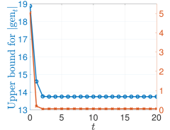
(a) $\sigma=0.6$

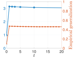
(b) $\sigma=3$

Figure 14: The comparison between the upper bound for $|\mathrm{gen}_{t}|$ and the empirical generalization error at each iteration $t$. The upper bounds are both for $d=2$.

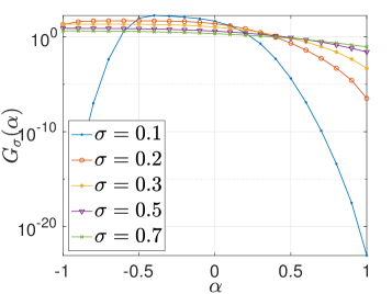
Figure 15: $G_{\sigma}(\alpha)$ versus $\alpha$ for different $\sigma$.

First, we compare the upper bounds for $|\mathrm{gen}_{0}|$ and $|\mathrm{gen}_{1}|$, as shown in Figures 13(a) and 13(b). For any fixed $\sigma$, when $n$ is sufficiently small, the upper bound for $|\mathrm{gen}_{0}|$ is greater than that for $|\mathrm{gen}_{1}|$. As $n$ increases, the upper bound for $|\mathrm{gen}_{1}|$ surpasses that of $|\mathrm{gen}_{0}|$, as shown in Figure 13(b). This is consistent with the intuition that when the labelled data is limited, using the unlabelled data can help improve the generalization performance. However, as the number of labelled data increases, using the unlabelled data may degrade the generalization performance, if the distributions corresponding to classes $+1$ and $-1$ have a large overlap. This is because the labelled data is already effective in learning the unknown parameter $\bm{\theta}_{t}$ well and additional pseudo-labelled data does not help to further boost the generalization performance. Furthermore, by comparing Figures 13(a) and 13(b), we can see that for smaller $\sigma$, the improvement from $|\mathrm{gen}_{0}|$ to $|\mathrm{gen}_{1}|$ is more pronounced. The intuition is that when $\sigma$ decreases, the data samples have smaller variance and thus the pseudo-labelling is more accurate. In this case, unlabelled data can improve the generalization performance. Let us examine the effect of $n$, the number of labelled training samples. Recall the Taylor expansion of $\alpha$ in (24). It can be seen that as $n$ increases, $\alpha$ converges to $1$ in probability. Suppose the dimension $d=2$ and $\bm{\mu}=(1,0)$. Then $\bm{\mu}^{\bot}=[0,\mu_{2}^{\bot}]$ where $\mu_{2}^{\bot}\sim\mathcal{N}(0,1)$. The upper bound for the absolute generalization error at $t=1$ can be rewritten as

$$|\mathrm{gen}_{1}|\lessapprox\frac{c_{2}-c_{1}}{\sqrt{2}}\int_{-\sqrt{2}}^{\sqrt{2}}\sqrt{\frac{n}{\pi\sigma^{2}}}\,e^{-\frac{ny^{2}}{\sigma^{2}}}\,\sqrt{G_{\sigma}(1-y^{2})}~{}\mathrm{d}y,$$ (132)

which is a decreasing function of $n$, as shown in Figures 13(a) and 13(b).

Second, in Figure 14(a), we plot the theoretical upper bound in (131) by ignoring $\epsilon$. Unfortunately it is computationally difficult to numerically calculate the bound in (131) for high dimensions $d$ (due to the need for high-dimensional numerical integration), but we can still gain insight from the result for $d=2$. It is shown that the upper bound for $|\mathrm{gen}_{t}|$ decreases as $t$ increases and finally converges to a non-zero constant. The gap between the upper bounds for $|\mathrm{gen}_{t}|$ and for $|\mathrm{gen}_{t+1}|$ decreases as $t$ increases and shrinks to almost 0 for $t\geq 2$. The intuition is that as $m\to\infty$, there are sufficient data at each iteration and the algorithm can converge at very early stage. In the empirical simulation, we let $n=10$, $d=50$, $\bm{\mu}=(1,0,\ldots,0)$ and iteratively run the self-training procedure for $20$ iterations and $2000$ rounds. We find that the behaviour of the empirical generalization error (the red ‘-x’ line) is similar to the theoretical upper bound (the blue ‘-o’ line), which almost converges to its final value at $t=2$. This result shows that the theoretical upper bound in (131) serves as a useful rule-of-thumb for how the generalization error changes over iterations. In Figure 14(b), we plot the theoretical bound and result from the empirical simulation based on the toy example for $d=2$ but larger $n$ and $\sigma$. This figure shows that when we increase $n$ and $\sigma$, using unlabelled data may not be able to improve the generalization performance. The intuition is that for $n$ large enough, merely using the labelled data can yield sufficiently low generalization error and for subsequent iterations with the pseudo-labelled data, the reduction in the test loss is negligible but the training loss will decrease more significantly (thus causing the generalization error to increase). When $\sigma$ is larger, the data samples have larger variance and the classes have a larger overlap, and thus, the initial parameter $\bm{\theta}_{0}$ learned by the labelled data cannot produce pseudo-labels with sufficiently high accuracy. Thus, the pseudo-labelled data cannot help to improve the generalization error significantly.

Remark 8 (Numerical plot of $G_{\sigma}(\cdot)$).

To gain more insight, we plot $G_{\sigma}(\alpha,\xi_{0},\bm{\mu}^{\bot})$ when $d=2$ and $\bm{\mu}=(1,0)$ in Figure 15. Under these settings, $G_{\sigma}(\alpha,\xi_{0},\bm{\mu}^{\bot})$ depends only on $\alpha$ and hence, we can rewrite it as $G_{\sigma}(\alpha)$. As shown in Figure 15 in Appendix D, for all $\sigma_{1}>\sigma_{2}$, there exists an $\alpha_{0}\in[-1,1]$ such that for all $\alpha\geq\alpha_{0}=\alpha_{0}(\sigma_{1},\sigma_{2})$, $G_{\sigma_{1}}(\alpha)>G_{\sigma_{2}}(\alpha)$. From (17), we can see that $\alpha$ is close to 1 of high probability, which means that $\sigma\mapsto G_{\sigma}(\alpha)$ is monotonically increasing in $\sigma$ with high probability. As a result, $\mathbb{E}_{\alpha}[\sqrt{G_{\sigma}(\alpha)}]$ increases as $\sigma$ increases. This is consistent with the intuition that when the training data has larger in-class variance, it is more difficult to generalize well.

Remark 9 (Discussion on Theorem 7).

As $n\to\infty$, $\bm{\theta}_{0}\to\bm{\mu}$ and $\alpha=\rho(\bm{\theta}_{0},\bm{\mu})\to 1$ almost surely, which means that the estimator converges to the optimal classifier for this bGMM. However, since there is no margin between two groups of data samples, the error probability $\Pr(\hat{Y}_{j}^{\prime}\neq Y_{j}^{\prime})\to\mathrm{Q}(1/\sigma)>0$ (which is the Bayes error rate) and the disintegrated KL-divergence $D_{\xi_{0},\bm{\mu}^{\bot}}(P_{\mathbf{X}_{j}^{\prime},\hat{Y}_{j}^{\prime}}\|P_{\mathbf{X},Y})$ between the estimated and underlying distributions cannot converge to $0$.

In the other extreme case, when $\alpha=\rho(\bm{\theta}_{0},\bm{\mu})=-1$ and $\bar{\bm{\theta}}_{0}=-\bm{\mu}$, the error probability $\Pr(\hat{Y}_{j}^{\prime}\neq Y_{j}^{\prime})=1-\mathrm{Q}(1/\sigma)>\frac{1}{2}$ (for all $\sigma>0$) and $D_{\xi_{0},\bm{\mu}^{\bot}}(P_{\mathbf{X}_{j}^{\prime},\hat{Y}_{j}^{\prime}}\|P_{\mathbf{X},Y})<\infty$, so in this other extreme (flipped) scenario, we have more mistakes than correct pseudo-labels. The reason why $D_{\alpha,\bm{\mu}^{\bot}}(P_{\mathbf{X}_{j}^{\prime},\hat{Y}_{j}^{\prime}}\|P_{\mathbf{X},Y})$ is finite is that when $P_{\mathbf{X},Y}(\mathbf{x},y)$ is small, it means that $\mathbf{x}$ is far from both $-\bm{\mu}$ and $\bm{\mu}$, and then $P_{\mathbf{X}}(\mathbf{x})$ is also small. Thus, $P_{\mathbf{X}_{j}^{\prime},\hat{Y}_{j}^{\prime}}(\mathbf{x},y)=P_{\hat{Y}_{j}^{\prime}|\mathbf{X}_{j}^{\prime}}(y|\mathbf{x})P_{\mathbf{X}}(\mathbf{x})$ is also small.

Appendix E Proof of Theorem 7

For simplicity, in the following, we abbreviate $\mathrm{gen}_{t}(P_{\mathbf{Z}},P_{\mathbf{X}},\{P_{\bm{\theta}_{k}|S_{\mathrm{l}},S_{\mathrm{u}}}\}_{k=0}^{t},\{f_{\bm{\theta}_{k}}\}_{k=0}^{t-1})$ as $\mathrm{gen}_{t}$.

1. Initial round $t=0$: Since $Y_{i}\mathbf{X}_{i}\overset{\text{i.i.d.}}{\sim}\mathcal{N}(\bm{\mu},\sigma^{2}\mathbf{I}_{d})$, we have $\bm{\theta}_{0}\sim\mathcal{N}(\bm{\mu},\frac{\sigma^{2}}{n}\mathbf{I}_{d})$ and for some constant $c\in\mathbb{R}_{+}$,

   $$\Pr(\bm{\theta}_{0}\in\Theta_{\bm{\mu},c})=\Pr(\|\bm{\theta}_{0}-\bm{\mu}\|_{\infty}\leq c)=\bigg{(}1-2\Phi\Big{(}-\frac{\sqrt{n}c}{\sigma}\Big{)}\bigg{)}^{d}=:1-\delta_{\sqrt{n}c,d}.$$ (133)

   By choosing $c$ large enough, $\delta_{\sqrt{n}c,d}$ can be made arbitrarily small. Consider $\tilde{\bm{\theta}}_{0}$ and $(\tilde{\mathbf{X}},\tilde{Y})$ as independent copies of $\bm{\theta}_{0}\sim Q_{\bm{\theta}_{0}}$ and $(\mathbf{X},Y)\sim P_{\mathbf{X},Y}=P_{Y}\otimes\mathcal{N}(Y\bm{\mu},\sigma^{2}I_{d})$, respectively, such that $P_{\tilde{\theta}_{0},\tilde{\mathbf{X}},\tilde{Y}}=Q_{\bm{\theta}_{0}}\otimes P_{\mathbf{X},Y}$. Then the probability that $l(\bm{\theta}_{0},(\mathbf{X},Y))\sim\mathrm{subG}((c_{2}-c_{1})/2)$ under $(\mathbf{X},Y)\sim P_{\mathbf{X},Y}$ is given as follows

   $$\Pr\bigg{(}\Lambda_{l(\tilde{\bm{\theta}}_{0},(\tilde{\mathbf{X}},\tilde{Y}))}(\lambda,\tilde{\bm{\theta}}_{0})\leq\frac{\lambda^{2}(c_{2}-c_{1})^{2}}{8}\bigg{)}$$ (134)

   $$\geq\Pr\bigg{(}\Lambda_{l(\tilde{\bm{\theta}}_{0},(\tilde{\mathbf{X}},\tilde{Y}))}(\lambda,\tilde{\bm{\theta}}_{0})\leq\frac{\lambda^{2}(c_{2}-c_{1})^{2}}{8}\text{ and }\tilde{\bm{\theta}}_{0}\in\Theta_{\bm{\mu},c}\bigg{)}$$ (135)

   $$=\Pr(\tilde{\bm{\theta}}_{0}\in\Theta_{\bm{\mu},c})\Pr\bigg{(}\Lambda_{l(\tilde{\bm{\theta}}_{0},(\tilde{\mathbf{X}},\tilde{Y}))}(\lambda,\tilde{\bm{\theta}}_{0})\leq\frac{\lambda^{2}(c_{2}-c_{1})^{2}}{8}\Big{|}\tilde{\bm{\theta}}_{0}\in\Theta_{\bm{\mu},c}\bigg{)}$$ (136)

   $$=(1-\delta_{\sqrt{n}c,d})(1-\delta_{r,d}),$$ (137)

   where (137) follows from (127) and (133).

   Fix some $d\in\mathbb{N}$, $\epsilon>0$ and $\delta\in(0,1)$. There exists $n_{0}(d,\delta)\in\mathbb{N}$, $r_{0}(d,\delta)\in\mathbb{R}_{+}$ such that for all $n>n_{0},r>r_{0}$, $\delta_{\sqrt{n}c,d}<\frac{\delta}{3}$, $\delta_{r,d}<\frac{\delta}{3}$, and then with probability at least $1-\delta$, the absolute generalization error can be upper bounded as follows

   $$|\mathrm{gen}_{0}|\leq\frac{1}{n}\sum_{i=1}^{n}\sqrt{\frac{(c_{2}-c_{1})^{2}}{2}I(\bm{\theta}_{0};\mathbf{X}_{i},Y_{i})}.$$ (138)

   Then mutual information can be calculated as follows

   $$I(\bm{\theta}_{0};\mathbf{X}_{i},Y_{i}) =h(\bm{\theta}_{0})-h(\bm{\theta}_{0}|\mathbf{X}_{i},Y_{i})$$ (139)

   $$=h\bigg{(}\frac{1}{n}\sum_{j=1}^{n}Y_{j}\mathbf{X}_{j}\bigg{)}-h\bigg{(}\frac{1}{n}\sum_{j=1}^{n}Y_{j}\mathbf{X}_{j}\bigg{|}\mathbf{X}_{i},Y_{i}\bigg{)}$$ (140)

   $$=\frac{d}{2}\log\bigg{(}\frac{2\pi e\sigma^{2}}{n}\bigg{)}-h\bigg{(}\frac{1}{n}\sum_{j\in[n],j\neq i}Y_{j}\mathbf{X}_{j}\bigg{)}$$ (141)

   $$=\frac{d}{2}\log\bigg{(}\frac{2\pi e\sigma^{2}}{n}\bigg{)}-\frac{d}{2}\log\bigg{(}\frac{2\pi e(n-1)\sigma^{2}}{n^{2}}\bigg{)}$$ (142)

   $$=\frac{d}{2}\log\frac{n}{n-1}.$$ (143)

   Thus we obtain (130).

2. Pseudo-label using $\bm{\theta}_{0}$: The same as those in Appendix C.

3. Iteration $t=1$: Recall $\bm{\theta}_{1}$ in (78), the new model parameter learned from the pseudo-labelled dataset $\hat{S}_{\mathrm{u},1}$.

   1. Recall the condition expectation of $\bm{\mu}_{1}^{\xi_{0},\bm{\mu}^{\bot}}$ in (94). The $l_{\infty}$ norm between $\bm{\mu}_{1}^{\xi_{0},\bm{\mu}^{\bot}}$ and $\bm{\mu}$ can be upper bounded by

      $$\|\bm{\mu}_{1}^{\xi_{0},\bm{\mu}^{\bot}}-\bm{\mu}\|_{\infty} \leq\sqrt{\bigg{(}-2\mathrm{Q}\bigg{(}\frac{\alpha}{\sigma}\bigg{)}+\frac{2\sigma\alpha}{\sqrt{2\pi}}\exp\bigg{(}-\frac{\alpha^{2}}{2\sigma^{2}}\bigg{)}\bigg{)}^{2}+\frac{2\sigma^{2}\beta^{2}}{\pi}\exp\bigg{(}-\frac{2\alpha^{2}}{2\sigma^{2}}\bigg{)}}$$ (144)

      $$<\sqrt{\bigg{(}2\Phi\bigg{(}\frac{1}{\sigma}\bigg{)}+\frac{2\sigma}{\sqrt{2\pi}}\bigg{)}^{2}+\frac{2\sigma^{2}}{\pi}}=:\tilde{c}_{1},$$ (145)

      where $\tilde{c}_{1}$ is a constant only dependent on $\sigma$.

   2. Next, we need to calculate the probability that $l(\bm{\theta}_{1},(\mathbf{X},Y))\sim\mathrm{subG}((c_{2}-c_{1}/2))$ under $(\mathbf{X},Y)\sim P_{\mathbf{X},Y}$.

      Let $\mathbf{V}_{i}=\operatorname{sgn}(\bar{\bm{\theta}}_{0}^{\top}\mathbf{X}_{i}^{\prime})\mathbf{X}_{i}^{\prime}-\bm{\mu}_{1}^{\xi_{0},\bm{\mu}^{\bot}}$. For any $k\in[d]$, let $V_{i,k}$, $\theta_{1,k}$, $\mu_{1,k}$ denote the $k$-th components of $\mathbf{V}_{i}$, $\bm{\theta}_{1}$ and $\bm{\mu}_{1}^{\xi_{0},\bm{\mu}^{\bot}}$, respectively. Recall the decompositions $\mathbf{X}_{i}^{\prime}=Y_{i}^{\prime}\bm{\mu}+\sigma\tilde{g}_{i}\bar{\bm{\theta}}_{0}+\sigma\tilde{\mathbf{g}}_{i}^{\bot}$ in (83) and $\bar{\bm{\theta}}_{0}\mathbf{X}_{i}^{\prime}=Y_{i}^{\prime}\alpha+\sigma\tilde{g}_{i}$ in (84). Suppose the basis of $\mathbb{R}^{d}$ is denoted by $B=\{\mathbf{v}_{1},\ldots,\mathbf{v}_{d}\}$ and let $\mathbf{v}_{1}=\bar{\bm{\theta}}_{0}$. Then we have

      $$\tilde{\mathbf{g}}_{i}^{\bot}=\tilde{g}_{i,2}^{\bot}\mathbf{v}_{2}+\ldots+\tilde{g}_{i,d}^{\bot}\mathbf{v}_{d},$$ (146)

      where $\tilde{g}_{i,k}^{\bot}\sim\mathcal{N}(0,1)$ for any $k\in[2:d]$ and $\{\tilde{g}_{i,k}\}_{k=2}^{d}$ are mutually independent. We also let $\bm{\mu}=(\mu_{0,1},\ldots,\mu_{0,d})$.

      Given any $(\xi_{0},\bm{\mu}^{\bot})$, the moment generating function (MGF) of $V_{i,1}$ is given as follows: for any $s_{1}>0$,

      $$\mathbb{E}_{V_{i,1}}[e^{s_{1}V_{i,1}}]$$

      $$=\mathrm{Q}\bigg{(}-\frac{\alpha}{\sigma}\bigg{)}\mathbb{E}_{\tilde{g}_{i}}\Big{[}e^{s_{1}(\mu_{0,1}-\mu_{1,1}+\sigma\tilde{g}_{i})}\Big{|}\tilde{g}_{i}>-\frac{\alpha}{\sigma}\Big{]}+\mathrm{Q}\bigg{(}\frac{\alpha}{\sigma}\bigg{)}\mathbb{E}_{\tilde{g}_{i}}\Big{[}e^{s_{1}(-\mu_{0,1}-\mu_{1,1}+\sigma\tilde{g}_{i})}\Big{|}\tilde{g}_{i}>\frac{\alpha}{\sigma}\Big{]}$$ (147)

      $$=e^{s_{1}(\mu_{0,1}-\mu_{1,1})}e^{\frac{\sigma^{2}s_{1}^{2}}{2}}\Phi\bigg{(}\frac{\alpha}{\sigma}+\sigma s_{1}\bigg{)}+e^{s_{1}(-\mu_{0,1}-\mu_{1,1})}e^{\frac{\sigma^{2}s_{1}^{2}}{2}}\Phi\bigg{(}-\frac{\alpha}{\sigma}+\sigma s_{1}\bigg{)}.$$ (148)

      The final equality follows from the fact that the MGF of a zero-mean univariate Gaussian truncated to $(a,b)$ is $e^{\sigma^{2}s^{2}/2}\Big{[}\frac{\Phi(b-\sigma s)-\Phi(a-\sigma s)}{\Phi(b)-\Phi(a)}\Big{]}$. The second derivative of $\log\mathbb{E}_{V_{i,1}}[e^{s_{1}V_{i,1}}]$ is given as

      $$\tilde{R}_{1}(s_{1}):=\frac{\mathrm{d}^{2}\log\mathbb{E}_{V_{i,1}}[e^{s_{1}V_{i,1}}]}{\mathrm{d}s_{1}^{2}}$$ (149)

      $$\leq\sigma^{2}+\frac{\mathrm{const.}}{\big{(}\Phi(\frac{\alpha}{\sigma}+\sigma s_{1})e^{s_{k}\mu_{0,k}}+\Phi(\frac{-\alpha}{\sigma}+\sigma s_{1})e^{-s_{k}\mu_{0,k}}\big{)}^{2}}<\infty.$$ (150)

      For $k\in[2:d]$ and any $s_{k}>0$, the MGF of $V_{i,k}$ is given as

      $$\mathbb{E}_{V_{i,k}}[e^{s_{k}V_{i,k}}]=\mathbb{E}_{\sigma\tilde{g}_{i,k}^{\bot},Y_{i}^{\prime}}\Big{[}e^{s_{k}(Y_{i}^{\prime}\mu_{0,k}-\mu_{1,k}+\sigma\tilde{g}_{i,k}^{\bot})}\Big{]}$$ (151)

      $$=Q\bigg{(}-\frac{\alpha}{\sigma}\bigg{)}e^{s_{k}(\mu_{0,k}-\mu_{1,k})}e^{\frac{\sigma^{2}s_{k}^{2}}{2}}+Q\bigg{(}\frac{\alpha}{\sigma}\bigg{)}e^{s_{k}(-\mu_{0,k}-\mu_{1,k})}e^{\frac{\sigma^{2}s_{k}^{2}}{2}},$$ (152)

      and the second derivative of $\log\mathbb{E}_{V_{i,k}}[e^{s_{k}V_{i,k}}]$ is given by

      $$\tilde{R}_{k}(s_{k}):=\frac{\mathrm{d}^{2}\log\mathbb{E}_{V_{i,k}}[e^{s_{k}V_{i,k}}]}{\mathrm{d}s_{k}^{2}}=\sigma^{2}+\frac{4\mu_{0,k}^{2}Q(-\frac{\alpha}{\sigma})Q(\frac{-\alpha}{\sigma})}{(Q(-\frac{\alpha}{\sigma})e^{s_{k}\mu_{0,k}}+Q(\frac{\alpha}{\sigma})e^{-s_{k}\mu_{0,k}})^{2}}.$$ (153)

      Fix $k\in[1:d]$. According to Taylor’s theorem, we have

      $$\log\mathbb{E}_{V_{i,k}}[e^{s_{k}V_{i,k}}]=\frac{\tilde{R}_{k}(\xi_{\mathrm{L},k})}{2}s_{k}^{2},$$ (154)

      for some $\xi_{\mathrm{L},k}\in(0,s_{k})$ and $\tilde{R}_{k}(\xi_{\mathrm{L},k})<\infty$. Then the Cramér transform of $\log\mathbb{E}_{V_{i,k}}[e^{s_{k}V_{i,k}}]$ can be lower bounded as follows: for any $\varepsilon>0$,

      $$\sup_{s_{k}>0}\Big{(}s_{k}\varepsilon-\log\mathbb{E}_{V_{i,k}}[e^{s_{k}V_{i,k}}]\Big{)}\geq\sup_{s_{k}>0}\Big{(}s_{k}\varepsilon-\frac{\tilde{R}_{k}(\xi_{\mathrm{L},k})s_{k}^{2}}{2}\Big{)}=\frac{\varepsilon^{2}}{2\tilde{R}_{k}(\xi_{\mathrm{L},k})}.$$ (155)

      Let $\tilde{R}^{*}=\max_{\xi_{0},\bm{\mu}^{\bot}}\min_{k\in[1:d]}\tilde{R}_{k}(\xi_{\mathrm{L},k})$, which is a finite constant only dependent on $\sigma$. Since $\{\operatorname{sgn}(\bar{\bm{\theta}}_{0}^{\top}\mathbf{X}_{i}^{\prime})\mathbf{X}_{i}^{\prime}\}_{i=1}^{m}$ are i.i.d. random variables conditioned on $(\xi_{0},\bm{\mu}^{\bot})$, by applying Chernoff-Cramér inequality, we have for all $\varepsilon>0$

      $$\mathbb{P}_{\xi_{0},\bm{\mu}^{\bot}}\Big{(}\|\bm{\theta}_{1}-\bm{\mu}_{1}^{\xi_{0},\bm{\mu}^{\bot}}\|_{\infty}>\varepsilon\Big{)}$$

      $$=\mathbb{P}_{\xi_{0},\bm{\mu}^{\bot}}\Big{(}\max_{k\in[1:d]}|\theta_{1,k}-\mu_{1,k}|>\varepsilon\Big{)}$$ (156)

      $$\leq\sum_{k=1}^{d}\mathbb{P}_{\xi_{0},\bm{\mu}^{\bot}}\Big{(}|\theta_{1,k}-\mu_{1,k}|>\varepsilon\Big{)}$$ (157)

      $$=\sum_{k=1}^{d}\mathbb{P}_{\xi_{0},\bm{\mu}^{\bot}}\bigg{(}\bigg{|}\frac{1}{m}\sum_{i=1}^{m}V_{i,k}\bigg{|}>\varepsilon\bigg{)}$$ (158)

      $$\leq\sum_{k=1}^{d}2\exp\Big{(}-m\sup_{s>0}\Big{(}s\varepsilon-\log\mathbb{E}_{V_{i,k}}[e^{sV_{i,k}}]\Big{)}\Big{)}$$ (159)

      $$\leq 2d\exp\bigg{(}-\frac{m\varepsilon^{2}}{2\tilde{R}^{*}}\bigg{)}$$ (160)

      $$=:\delta_{m,\varepsilon,d},$$ (161)

      where $\delta_{m,\varepsilon,d}\xrightarrow{\text{a.s.}}0$ as $m\to\infty$ and does not depend on $\xi_{0},\bm{\mu}^{\bot}$.

      Choose some $c\in(\tilde{c}_{1},\infty)$ ($\tilde{c}_{1}$ defined in (145)). We have

      $$\mathbb{P}_{\xi_{0},\bm{\mu}^{\bot}}\big{(}\bm{\theta}_{1}\in\Theta_{\bm{\mu},c})\geq\mathbb{P}_{\xi_{0},\bm{\mu}^{\bot}}(\|\bm{\theta}_{1}-\bm{\mu}_{1}^{\xi_{0},\bm{\mu}^{\bot}}\|_{\infty}\leq c-\tilde{c}_{1}\big{)}\geq 1-\delta_{m,c-\tilde{c}_{1},d}.$$ (162)

      Consider $\tilde{\bm{\theta}}_{1}$ as an independent copy of $\bm{\theta}_{1}$ and independent of $(\tilde{\mathbf{X}},\tilde{Y})$. Then the probability that $l(\bm{\theta}_{1},(\mathbf{X},Y))\sim\mathrm{subG}((c_{2}-c_{1})/2)$ under $(\mathbf{X},Y)\sim P_{\mathbf{X},Y}$ is given as follows

      $$\mathbb{P}_{\xi_{0},\bm{\mu}^{\bot}}\bigg{(}\Lambda_{l(\tilde{\bm{\theta}}_{1},(\tilde{\mathbf{X}},\tilde{Y}))}(\lambda,\tilde{\bm{\theta}}_{1})\leq\frac{\lambda^{2}(c_{2}-c_{1})^{2}}{8}\bigg{)}$$ (163)

      $$\geq\mathbb{P}_{\xi_{0},\bm{\mu}^{\bot}}(\tilde{\bm{\theta}}_{1}\in\Theta_{\bm{\mu},c})\mathbb{P}_{\xi_{0},\bm{\mu}^{\bot}}\bigg{(}\Lambda_{l(\tilde{\bm{\theta}}_{1},(\tilde{\mathbf{X}},\tilde{Y}))}(\lambda,\tilde{\bm{\theta}}_{1})\leq\frac{\lambda^{2}(c_{2}-c_{1})^{2}}{8}\Big{|}\tilde{\bm{\theta}}_{1}\in\Theta_{\bm{\mu},c}\bigg{)}$$ (164)

      $$=(1-\delta_{m,c,d})(1-\delta_{r,d}).$$ (165)

   Thus, for some $c\in(\tilde{c}_{1},\infty)$, with probability at least $(1-\delta_{m,c-\tilde{c}_{1},d})(1-\delta_{r,d})$, the absolute generalization error can be upper bounded as follows:

   $$|\mathrm{gen}_{1}|=|\mathbb{E}[L_{P_{\mathbf{Z}}}(\bm{\theta}_{1})-L_{\hat{S}_{\mathrm{u},1}}(\bm{\theta}_{1})]|$$ (166)

   $$=\bigg{|}\frac{1}{m}\sum_{i=1}^{m}\mathbb{E}_{\xi_{0},\bm{\mu}^{\bot}}\bigg{[}\mathbb{E}\left[l(\bm{\theta}_{1},(\mathbf{X},Y))-l(\bm{\theta}_{1},(\mathbf{X}^{\prime}_{i},\hat{Y}_{i}^{\prime}))|\xi_{0},\bm{\mu}^{\bot}\right]\bigg{]}\bigg{|}$$ (167)

   $$\leq\frac{1}{m}\sum_{i=1}^{m}\mathbb{E}_{\xi_{0},\bm{\mu}^{\bot}}\bigg{[}\sqrt{\frac{(c_{2}-c_{1})^{2}}{2}\Big{(}I_{\xi_{0},\bm{\mu}^{\bot}}(\bm{\theta}_{1},(\mathbf{X}^{\prime}_{i},\hat{Y}_{i}^{\prime}))+D_{\xi_{0},\bm{\mu}^{\bot}}(P_{\mathbf{X}^{\prime}_{i},\hat{Y}_{i}^{\prime}}\|P_{\mathbf{X},Y})\Big{)}}~{}\bigg{]},$$ (168)

   where $P_{\bm{\theta}_{1},(\mathbf{X},Y)|\xi_{0},\bm{\mu}^{\bot}}=Q_{\bm{\theta}_{1}|\xi_{0},\bm{\mu}^{\bot}}\otimes P_{\mathbf{X},Y}$ and $Q_{\bm{\theta}_{1}|\xi_{0},\bm{\mu}^{\bot}}$ denotes the marginal distribution of $\bm{\theta}_{1}$ under parameters $(\xi_{0},\bm{\mu}^{\bot})$.

   In the following, we derive closed-form expressions of the mutual information and KL-divergence in (168). For any $j\in[1:m]$:

   • Calculate $I_{\xi_{0},\bm{\mu}^{\bot}}(\bm{\theta}_{1};\mathbf{X}^{\prime}_{j},\hat{Y}_{j}^{\prime})$: For arbitrary random variables $X$ and $U$, we define the disintegrated conditional differential entropy of $X$ given $U$ as

     $$h_{U}(X):=h(P_{X|U}).$$ (169)

     This is a $\sigma(U)$-measurable random variable. Conditioned on a certain pair $(\xi_{0},\bm{\mu}^{\bot})$, the mutual information between $\bm{\theta}_{1}$ and $(\mathbf{X}^{\prime}_{i},\hat{Y}_{i}^{\prime})$ is

     $$I_{\xi_{0},\bm{\mu}^{\bot}}(\bm{\theta}_{1};\mathbf{X}^{\prime}_{i},\hat{Y}_{i}^{\prime})$$

     $$=h_{\xi_{0},\bm{\mu}^{\bot}}\bigg{(}\frac{1}{m}\sum_{i=1}^{m}\operatorname{sgn}(\bm{\theta}_{0}^{\top}\mathbf{X}^{\prime}_{i})\mathbf{X}^{\prime}_{i}\bigg{)}-h_{\xi_{0},\bm{\mu}^{\bot}}\bigg{(}\frac{1}{m}\sum_{j=1}^{m}\hat{Y}_{j}^{\prime}\mathbf{X}^{\prime}_{j}\bigg{|}\mathbf{X}^{\prime}_{i},\hat{Y}_{i}^{\prime}\bigg{)}$$ (170)

     $$=h_{\xi_{0},\bm{\mu}^{\bot}}\bigg{(}\frac{1}{m}\sum_{i=1}^{m}\operatorname{sgn}(\bm{\theta}_{0}^{\top}\mathbf{X}^{\prime}_{i})\mathbf{X}^{\prime}_{i}\bigg{)}-h_{\xi_{0},\bm{\mu}^{\bot}}\bigg{(}\frac{1}{m}\sum_{j\in[m],j\neq i}\operatorname{sgn}(\bm{\theta}_{0}^{\top}\mathbf{X}^{\prime}_{j})\mathbf{X}^{\prime}_{j}\bigg{)}$$ (171)

     $$=h_{\xi_{0},\bm{\mu}^{\bot}}\bigg{(}\frac{1}{m}\sum_{i=1}^{m}\operatorname{sgn}(\bm{\theta}_{0}^{\top}\mathbf{X}^{\prime}_{i})\mathbf{X}^{\prime}_{i}\bigg{)}$$

     $$\quad-h_{\xi_{0},\bm{\mu}^{\bot}}\bigg{(}\frac{1}{m-1}\sum_{j\in[m],j\neq i}\operatorname{sgn}(\bm{\theta}_{0}^{\top}\mathbf{X}^{\prime}_{j})\mathbf{X}^{\prime}_{j}\bigg{)}-d\log\frac{m-1}{m}.$$ (172)

     As $m\to\infty$, $I_{\xi_{0},\bm{\mu}^{\bot}}(\bm{\theta}_{1};\mathbf{X}^{\prime}_{i},\hat{Y}_{i}^{\prime})\to 0$ almost surely and hence, in probability. Thus, for any $\epsilon>0$, and there exists $m_{0}(\epsilon,d,\delta)\in\mathbb{N}$ such that for all $m>m_{0}$,

     $$\mathbb{P}_{\xi_{0},\bm{\mu}^{\bot}}(I_{\xi_{0},\bm{\mu}^{\bot}}(\bm{\theta}_{1};\mathbf{X}^{\prime}_{i},\hat{Y}_{i}^{\prime})>\epsilon)\leq\delta.$$ (173)

   • Calculate $D_{\xi_{0},\bm{\mu}^{\bot}}(P_{\mathbf{X}_{j}^{\prime},\hat{Y}_{j}^{\prime}}\|P_{\mathbf{X},Y})$: First of all, since $P_{\hat{Y}_{j}^{\prime}}=P_{Y}$ (cf. (77)) regardless of the values of $(\xi_{0},\bm{\mu}^{\bot})$, the disintegrated conditional KL-divergence can be rewritten as

     $$D_{\xi_{0},\bm{\mu}^{\bot}}(P_{\mathbf{X}_{j}^{\prime},\hat{Y}_{j}^{\prime}}\|P_{\mathbf{X},Y})$$

     $$=P_{\hat{Y}_{j}^{\prime}}(-1)D_{\xi_{0},\bm{\mu}^{\bot}}(P_{\mathbf{X}_{j}^{\prime}|\hat{Y}_{j}^{\prime}=-1}\|P_{\mathbf{X}|Y=-1})+P_{\hat{Y}_{j}^{\prime}}(1)D_{\xi_{0},\bm{\mu}^{\bot}}(P_{\mathbf{X}_{j}^{\prime}|\hat{Y}_{j}^{\prime}=1}\|P_{\mathbf{X}|Y=1}).$$ (174)

     Recall the decomposition of a Gaussian vector $\tilde{\mathbf{g}}_{j}\sim\mathcal{N}(0,\mathbf{I}_{d})$ in (82). Note that $\operatorname{rank}(\operatorname{\mathsf{Cov}}(\tilde{\mathbf{g}}_{j}^{\bot}))=\operatorname{rank}(\mathbf{I}_{d}-\bar{\bm{\theta}}\bar{\bm{\theta}}^{\top})=d-1$.

     For any pair of labelled data sample $(\mathbf{X},Y)$, from (83), we similarly decompose $\mathbf{X}$ as $\mathbf{X}=Y\bm{\mu}+\sigma(\tilde{g}\bar{\bm{\theta}}_{0}+\tilde{\mathbf{g}}^{\bot})$, where $\tilde{g}\sim\mathcal{N}(0,1)$ and $\tilde{\mathbf{g}}^{\bot}\sim\mathcal{N}(0,\mathbf{I}_{d}-\bar{\bm{\theta}}_{0}\bar{\bm{\theta}}_{0}^{\top})$. Let $p_{\tilde{g}}$ and $p_{\tilde{\mathbf{g}}^{\bot}}$ denote the probability density functions of $\tilde{g}$ and $\tilde{\mathbf{g}}^{\bot}$, respectively. For any $\mathbf{x}=\bm{\mu}+\sigma(u\bar{\bm{\theta}}_{0}+\mathbf{u}^{\perp})\in\mathbb{R}^{d}$, the joint probability distribution at $(\mathbf{X},Y)=(\mathbf{x},1)$ is given by

     $$P_{\mathbf{X},Y}(\mathbf{x},1) =P_{Y}(1)p_{\bm{\mu}}(\mathbf{x}|1)$$

     $$=\frac{P_{Y}(1)}{\sqrt{(2\pi)^{d}}\sigma^{d}}\exp\bigg{(}-\frac{1}{2\sigma^{2}}(\mathbf{x}-y\bm{\mu})^{\top}(\mathbf{x}-y\bm{\mu})\bigg{)}$$ (175)

     $$=\frac{P_{Y}(1)}{\sqrt{(2\pi)^{d}}\sigma^{d}}\exp\bigg{(}-\frac{1}{2\sigma^{2}}(\sigma u\bar{\bm{\theta}_{0}}+\sigma\mathbf{u}^{\bot})^{\top}(\sigma u\bar{\bm{\theta}_{0}}+\sigma\mathbf{u}^{\bot})\bigg{)}$$ (176)

     $$=\frac{P_{Y}(y)}{\sqrt{(2\pi)^{d}}\sigma^{d}}\exp\bigg{(}-\frac{u^{2}}{2}\bigg{)}\exp\bigg{(}-\frac{(\mathbf{u}^{\bot})^{\top}\mathbf{u}^{\bot}}{2}\bigg{)}$$ (177)

     $$=P_{Y}(1)p_{\tilde{g}}(u)p_{\tilde{\mathbf{g}}^{\bot}}(\mathbf{u}^{\bot}).$$ (178)

     Similarly, for any $\mathbf{x}=-\bm{\mu}+\sigma(u\bar{\bm{\theta}}_{0}+\mathbf{u}^{\perp})\in\mathbb{R}^{d}$, the joint probability density evaluated at $(X,Y)=(\mathbf{x},-1)$ is given by

     $$P_{\mathbf{X},Y}(\mathbf{x},-1)=P_{Y}(-1)p_{\bm{\mu}}(\mathbf{x}|-1)=P_{Y}(-1)p_{\tilde{g}}(u)p_{\tilde{\mathbf{g}}^{\bot}}(\mathbf{u}^{\bot}).$$ (179)

     Second, we have $P_{\mathbf{X}_{j}^{\prime}|\hat{Y}_{j}^{\prime}}=\sum_{y\in\{-1,+1\}}P_{\mathbf{X}_{j}^{\prime}|\hat{Y}_{j}^{\prime},Y_{j}^{\prime}=y}P_{Y_{j}^{\prime}=y|\hat{Y}_{j}^{\prime}}$. The conditional probability distribution $P_{Y_{j}^{\prime}|\hat{Y}_{j}^{\prime}}$ can be calculated as follows

     $$P_{Y_{j}^{\prime}|\hat{Y}_{j}^{\prime}}=\frac{P_{\hat{Y}_{j}^{\prime}|Y_{j}^{\prime}}P_{Y_{j}^{\prime}}}{P_{\hat{Y}_{j}^{\prime}}}=P_{\hat{Y}_{j}^{\prime}|Y_{j}^{\prime}},$$ (180)

     where the last equality follows since $P_{Y_{j}^{\prime}}(-1)=P_{Y_{j}^{\prime}}(1)=P_{\hat{Y}_{j}^{\prime}}(-1)=P_{\hat{Y}_{j}^{\prime}}(1)=1/2$. Since $\hat{Y}_{j}^{\prime}=\operatorname{sgn}(Y_{j}^{\prime}\alpha+\sigma\tilde{g}_{j})$ (cf. (84)), we have

     $$P_{\hat{Y}_{j}^{\prime}|Y_{j}^{\prime}}(-1|-1)=\Pr(Y_{j}^{\prime}\alpha+\sigma\tilde{g}_{j}<0|Y_{j}^{\prime}=-1)=\mathrm{Q}\bigg{(}-\frac{\alpha}{\sigma}\bigg{)},$$ (181)

     and similarly,

     $$P_{\hat{Y}_{j}^{\prime}|Y_{j}^{\prime}}(1|-1)=\mathrm{Q}\bigg{(}\frac{\alpha}{\sigma}\bigg{)},\;\;\;\;P_{\hat{Y}_{j}^{\prime}|Y_{j}^{\prime}}(-1|1)=\mathrm{Q}\bigg{(}\frac{\alpha}{\sigma}\bigg{)},\;\;\;\;P_{\hat{Y}_{j}^{\prime}|Y_{j}^{\prime}}(1|1)=\mathrm{Q}\bigg{(}-\frac{\alpha}{\sigma}\bigg{)}.$$ (182)

     Thus, we conclude that

     $$P_{Y_{j}^{\prime}|\hat{Y}_{j}^{\prime}}(y_{j}^{\prime}|\hat{y}_{j}^{\prime})=\left\{\begin{array}[]{cc}\mathrm{Q}(-\frac{\alpha}{\sigma})&y_{j}^{\prime}=\hat{y}_{j}^{\prime}\\ \mathrm{Q}(\frac{\alpha}{\sigma})&y_{j}^{\prime}\neq\hat{y}_{j}^{\prime}.\end{array}\right.$$ (185)

     To calculate the conditional probability distribution $P_{\mathbf{X}_{j}^{\prime}|\hat{Y}_{j}^{\prime},Y_{j}^{\prime}}$, recall the decomposition of $\mathbf{X}_{j}^{\prime}$ and $\bar{\bm{\theta}}_{0}^{\top}\mathbf{X}_{j}^{\prime}$ in (83) and (84). Since the event $\{\hat{Y}_{j}^{\prime}=-1,Y_{j}^{\prime}=-1\}$ is equivalent to $\{\tilde{g}_{j}<\alpha/\sigma\}$ and $\tilde{g}_{j}\sim\mathcal{N}(0,1)$, the conditional density of $\tilde{g}_{j}$ given $\hat{Y}_{j}^{\prime}=-1,Y_{j}^{\prime}=-1$ is given by

     $$p_{\tilde{g}_{j}|\hat{Y}_{j}^{\prime},Y_{j}^{\prime}}(u|-1,-1)=p_{\tilde{g}_{j}|\tilde{g}_{j}\leq\alpha/\sigma}(u)=\frac{\text{1}\{u\leq\alpha/\sigma\}p_{\tilde{g}_{j}}(u)}{\Phi(\alpha/\sigma)},\quad\forall u\in\mathbb{R}.$$ (186)

     Similarly, for any $u\in\mathbb{R}$

     $$p_{\tilde{g}_{j}|\hat{Y}_{j}^{\prime},Y_{j}^{\prime}}(u|-1,1) =p_{\tilde{g}_{j}|\tilde{g}_{j}\leq-\alpha/\sigma}(u)=\frac{\text{1}\{u\leq-\alpha/\sigma\}f_{\tilde{g}_{j}}(u)}{\Phi(-\alpha/\sigma)},$$ (187)

     $$p_{\tilde{g}_{j}|\hat{Y}_{j}^{\prime},Y_{j}^{\prime}}(u|1,-1) =p_{\tilde{g}_{j}|\tilde{g}_{j}>\alpha/\sigma}(u)=\frac{\text{1}\{z>\alpha/\sigma\}f_{\tilde{g}_{j}}(u)}{\mathrm{Q}(\alpha/\sigma)},$$ (188)

     $$p_{\tilde{g}_{j}|\hat{Y}_{j}^{\prime},Y_{j}^{\prime}}(u|1,1) =p_{\tilde{g}_{j}|\tilde{g}_{j}>-\alpha/\sigma}(u)=\frac{\text{1}\{u>-\alpha/\sigma\}p_{\tilde{g}_{j}}(u)}{\mathrm{Q}(-\alpha/\sigma)}.$$ (189)

     For any $\mathbf{x}=\bm{\mu}+\sigma(u\bar{\bm{\theta}}_{0}+\mathbf{u}^{\perp})\in\mathbb{R}^{d}$, given $\hat{Y}_{j}^{\prime}=1,Y_{j}^{\prime}=1$, the conditional probability distribution at $\mathbf{X}_{j}^{\prime}=\mathbf{x}$ is given by

     $$P_{\mathbf{X}_{j}^{\prime}|\hat{Y}_{j}^{\prime},Y_{j}^{\prime}}(\mathbf{x}|1,1) =P_{\bm{\mu}+\sigma\tilde{g}_{j}\bar{\bm{\theta}}_{0}+\sigma\tilde{\mathbf{g}}_{j}^{\bot}|\hat{Y}_{j}^{\prime},Y_{j}^{\prime}}(\bm{\mu}+\sigma(u\bar{\bm{\theta}}_{0}+\mathbf{u}^{\perp})|1,1)$$ (190)

     $$=P_{\sigma\tilde{g}_{j}\bar{\bm{\theta}}_{0}+\sigma\tilde{\mathbf{g}}_{j}^{\bot}|\hat{Y}_{j}^{\prime},Y_{j}^{\prime}}(\sigma(u\bar{\bm{\theta}}_{0}+\mathbf{u}^{\perp})|1,1)$$ (191)

     $$=p_{\tilde{g}_{j}|\hat{Y}_{j}^{\prime},Y_{j}^{\prime}}(u|1,1)p_{\tilde{\mathbf{g}}_{j}^{\bot}}(\mathbf{u}^{\bot}),$$ (192)

     where (192) follows since $\tilde{g}_{j}$ and $\tilde{\mathbf{g}}_{j}^{\bot}$ are mutually independent and $\bar{\bm{\theta}}_{0}\perp\tilde{\mathbf{g}}_{j}^{\bot}$.

     Since we can decompose $2\bm{\mu}/\sigma$ as

     $$\frac{2\bm{\mu}}{\sigma}=\frac{2\alpha\bar{\bm{\theta}}_{0}+2\beta^{2}\bm{\mu}-2\alpha\beta\bm{\upsilon}}{\sigma}=\frac{2\alpha}{\sigma}\bar{\bm{\theta}}_{0}+\bar{\bm{\theta}}_{0}^{\bot},$$ (193)

     given $\hat{Y}_{j}^{\prime}=1,Y_{j}^{\prime}=-1$, the conditional probability distribution at $\mathbf{X}_{j}^{\prime}=\mathbf{x}$ is given by

     $$P_{\mathbf{X}_{j}^{\prime}|\hat{Y}_{j}^{\prime},Y_{j}^{\prime}}(\mathbf{x}|1,-1) =P_{-\bm{\mu}+\sigma\tilde{g}_{j}\bar{\bm{\theta}}_{0}+\sigma\tilde{\mathbf{g}}_{j}^{\bot}|\hat{Y}_{j}^{\prime},Y_{j}^{\prime}}(\bm{\mu}+\sigma(u\bar{\bm{\theta}}_{0}+\mathbf{u}^{\perp})|1,-1)$$ (194)

     $$=P_{\sigma\tilde{g}_{j}\bar{\bm{\theta}}_{0}+\sigma\tilde{\mathbf{g}}_{j}^{\bot}|\hat{Y}_{j}^{\prime},Y_{j}^{\prime}}\Big{(}\sigma\Big{(}\frac{2\bm{\mu}}{\sigma}+u\bar{\bm{\theta}}_{0}+\mathbf{u}^{\perp}\Big{)}\Big{|}1,-1\Big{)}$$ (195)

     $$=p_{\tilde{g}_{j}|\hat{Y}_{j}^{\prime},Y_{j}^{\prime}}\Big{(}u+\frac{2\alpha}{\sigma}\Big{|}1,-1\Big{)}p_{\tilde{\mathbf{g}}_{j}^{\bot}}(\mathbf{u}^{\bot}+\bar{\bm{\theta}}_{0}^{\bot}).$$ (196)

     Similarly, for any $\mathbf{x}=-\bm{\mu}+\sigma(u\bar{\bm{\theta}}_{0}+\mathbf{u}^{\perp})\in\mathbb{R}^{d}$, given $\hat{Y}_{j}^{\prime}=-1,Y_{j}^{\prime}=1$, the conditional distribution at $\mathbf{X}_{j}^{\prime}=\mathbf{x}$ is given by

     $$P_{\mathbf{X}_{j}^{\prime}|\hat{Y}_{j}^{\prime},Y_{j}^{\prime}}(\mathbf{x}|-1,1) =P_{\bm{\mu}+\sigma\tilde{g}_{j}\bar{\bm{\theta}}_{0}+\sigma\tilde{\mathbf{g}}_{j}^{\bot}|\hat{Y}_{j}^{\prime},Y_{j}^{\prime}}(-\bm{\mu}+\sigma(u\bar{\bm{\theta}}_{0}+\mathbf{u}^{\perp})|-1,1)$$ (197)

     $$=p_{\tilde{g}_{j}|\hat{Y}_{j}^{\prime},Y_{j}^{\prime}}\Big{(}u-\frac{2\alpha}{\sigma}\Big{|}-1,1\Big{)}p_{\tilde{\mathbf{g}}_{j}^{\bot}}(\mathbf{u}^{\bot}-\bar{\bm{\theta}}_{0}^{\bot});$$ (198)

     and given $\hat{Y}_{j}^{\prime}=-1,Y_{j}^{\prime}=-1$,

     $$P_{\mathbf{X}_{j}^{\prime}|\hat{Y}_{j}^{\prime},Y_{j}^{\prime}}(\mathbf{x}|-1,-1) =P_{-\bm{\mu}+\sigma\tilde{g}_{j}\bar{\bm{\theta}}_{0}+\sigma\tilde{\mathbf{g}}_{j}^{\bot}|\hat{Y}_{j}^{\prime},Y_{j}^{\prime}}(-\bm{\mu}+\sigma(u\bar{\bm{\theta}}_{0}+\mathbf{u}^{\perp})|-1,-1)$$ (199)

     $$=p_{\tilde{g}_{j}|\hat{Y}_{j}^{\prime},Y_{j}^{\prime}}(u|-1,-1)p_{\tilde{\mathbf{g}}_{j}^{\bot}}(\mathbf{u}^{\bot}).$$ (200)

     Furthermore, for any $\mathbf{x}=-\bm{\mu}+\sigma(u\bar{\bm{\theta}}_{0}+\mathbf{u}^{\perp})\in\mathbb{R}^{d}$, we have

     $$P_{\mathbf{X}_{j}^{\prime}|\hat{Y}_{j}^{\prime}=-1}(\mathbf{x}) =\sum_{y\in\{-1,+1\}}P_{\mathbf{X}_{j}^{\prime}|\hat{Y}_{j}^{\prime}=-1,Y_{j}^{\prime}=y}(\mathbf{x})P_{Y_{j}^{\prime}|\hat{Y}_{j}^{\prime}=-1}(y)$$ (201)

     $$=P_{Y_{j}^{\prime}|\hat{Y}_{j}^{\prime}=-1}(1)p_{\tilde{g}_{j}|\hat{Y}_{j}^{\prime},Y_{j}^{\prime}}\Big{(}u-\frac{2\alpha}{\sigma}\Big{|}-1,1\Big{)}p_{\tilde{\mathbf{g}}_{j}^{\bot}}(\mathbf{u}^{\bot}-\bar{\bm{\theta}}_{0}^{\bot})$$

     $$\quad+P_{Y_{j}^{\prime}|\hat{Y}_{j}^{\prime}=-1}(-1)p_{\tilde{g}_{j}|\hat{Y}_{j}^{\prime},Y_{j}^{\prime}}(u|-1,-1)p_{\tilde{\mathbf{g}}_{j}^{\bot}}(\mathbf{u}^{\bot})$$ (202)

     $$=\text{1}\Big{\{}u\leq\frac{\alpha}{\sigma}\Big{\}}p_{\tilde{g}_{j}}\Big{(}u-\frac{2\alpha}{\sigma}\Big{)}p_{\tilde{\mathbf{g}}_{j}^{\bot}}(\mathbf{u}^{\bot}-\bar{\bm{\theta}}_{0}^{\bot})+\text{1}\Big{\{}u\leq\frac{\alpha}{\sigma}\Big{\}}p_{\tilde{g}_{j}}(u)p_{\tilde{\mathbf{g}}_{j}^{\bot}}(\mathbf{u}^{\bot});$$ (203)

     for any $\mathbf{x}=\bm{\mu}+\sigma(u\bar{\bm{\theta}}_{0}+\mathbf{u}^{\perp})\in\mathbb{R}^{d}$, we have

     $$P_{\mathbf{X}_{j}^{\prime}|\hat{Y}_{j}^{\prime}=1}(\mathbf{x})=\sum_{y\in\{-1,+1\}}P_{\mathbf{X}_{j}^{\prime}|\hat{Y}_{j}^{\prime}=1,Y_{j}^{\prime}=y}(\mathbf{x})P_{Y_{j}^{\prime}|\hat{Y}_{j}^{\prime}=1}(y)$$ (204)

     $$=\text{1}\Big{\{}u>-\frac{\alpha}{\sigma}\Big{\}}p_{\tilde{g}_{j}}\Big{(}u+\frac{2\alpha}{\sigma}\Big{)}p_{\tilde{\mathbf{g}}_{j}^{\bot}}(\mathbf{u}^{\bot}+\bar{\bm{\theta}}_{0}^{\bot})+\text{1}\Big{\{}u>-\frac{\alpha}{\sigma}\Big{\}}p_{\tilde{g}_{j}}(u)p_{\tilde{\mathbf{g}}_{j}^{\bot}}(\mathbf{u}^{\bot}).$$ (205)

     Define the set $\mathcal{U}_{0}^{\bot}(\xi_{0},\bm{\mu}^{\bot}):=\{\mathbf{u}^{\bot}\in\mathbb{R}^{d}:\mathbf{u}^{\bot}\perp\bm{\theta}_{0}\}$. We also use $\mathcal{U}_{0}^{\bot}$ to represent $\mathcal{U}_{0}^{\bot}(\xi_{0},\bm{\mu}^{\bot})$, if there is no risk of confusion. Recall (128) and note that $\int_{\mathcal{U}_{0}^{\bot}}p_{\tilde{\mathbf{g}}^{\bot}}(\mathbf{u}^{\bot})\mathrm{d}\mathbf{u}^{\bot}=1$. Finally, the KL-divergence is given by

     $$D_{\xi_{0},\bm{\mu}^{\bot}}(P_{\mathbf{X}_{j}^{\prime}|\hat{Y}_{j}^{\prime}=-1}\|P_{\mathbf{X}|Y=-1})$$

     $$=\int_{\mathcal{U}_{0}^{\bot}}\int^{\frac{\alpha}{\sigma}}_{-\infty}\bigg{(}p_{\tilde{g}_{j}}\Big{(}u-\frac{2\alpha}{\sigma}\Big{)}p_{\tilde{\mathbf{g}}_{j}^{\bot}}(\mathbf{u}^{\bot}-\bar{\bm{\theta}}_{0}^{\bot})+p_{\tilde{g}_{j}}(u)p_{\tilde{\mathbf{g}}_{j}^{\bot}}(\mathbf{u}^{\bot})\bigg{)}$$

     $$\qquad\times\log\bigg{(}1+\frac{p_{\tilde{g}_{j}}\Big{(}u-\frac{2\alpha}{\sigma}\Big{)}p_{\tilde{\mathbf{g}}_{j}^{\bot}}(\mathbf{u}^{\bot}-\bar{\bm{\theta}}_{0}^{\bot})}{p_{\tilde{g}_{j}}(u)p_{\tilde{\mathbf{g}}_{j}^{\bot}}(\mathbf{u}^{\bot})}\bigg{)}\,\mathrm{d}u\,\mathrm{d}\mathbf{u}^{\bot}=G_{\sigma}(\alpha,\xi_{0},\bm{\mu}^{\bot})$$ (206)

     and

     $$D_{\xi_{0},\bm{\mu}^{\bot}}(P_{\mathbf{X}_{j}^{\prime}|\hat{Y}_{j}^{\prime}=1}\|P_{\mathbf{X}|Y=1})$$

     $$=\int_{\mathcal{U}_{0}^{\bot}}\int_{-\frac{\alpha}{\sigma}}^{+\infty}\bigg{(}p_{\tilde{g}_{j}}\Big{(}u+\frac{2\alpha}{\sigma}\Big{)}p_{\tilde{\mathbf{g}}_{j}^{\bot}}(\mathbf{u}^{\bot}+\bar{\bm{\theta}}_{0}^{\bot})+p_{\tilde{g}_{j}}(u)p_{\tilde{\mathbf{g}}_{j}^{\bot}}(\mathbf{u}^{\bot})\bigg{)}$$

     $$\qquad\times\log\bigg{(}1+\frac{p_{\tilde{g}_{j}}\Big{(}u+\frac{2\alpha}{\sigma}\Big{)}p_{\tilde{\mathbf{g}}_{j}^{\bot}}(\mathbf{u}^{\bot}+\bar{\bm{\theta}}_{0}^{\bot})}{p_{\tilde{g}_{j}}(u)p_{\tilde{\mathbf{g}}_{j}^{\bot}}(\mathbf{u}^{\bot})}\bigg{)}\,\mathrm{d}u\,\mathrm{d}\mathbf{u}^{\bot}=G_{\sigma}(\alpha,\xi_{0},\bm{\mu}^{\bot}),$$ (207)

     where (207) follows from since $p_{\tilde{g}_{j}}$ and $p_{\tilde{\mathbf{g}}_{j}^{\bot}}$ are zero-mean Gaussian distributions. Then from (174), we have

     $$D_{\xi_{0},\bm{\mu}^{\bot}}(P_{\mathbf{X}_{j}^{\prime},\hat{Y}_{j}^{\prime}}\|P_{\mathbf{X},Y})=G_{\sigma}(\alpha,\xi_{0},\bm{\mu}^{\bot}).$$ (208)

   Thus, by combining the aforementioned results, we get the closed-form expression of the upper bound for $|\mathrm{gen}_{1}|$. Indeed, if we fix some $d\in\mathbb{N}$, $\epsilon>0$ and $\delta\in(0,1)$, there exists $n_{0}(d,\delta)\in\mathbb{N}$, $m_{0}(\epsilon,d,\delta)\in\mathbb{N}$, $c_{0}(d,\delta)\in(\tilde{c}_{1},\infty)$, $r_{0}(d,\delta)\in\mathbb{R}_{+}$ such that for all $n>n_{0},m>m_{0},c>c_{0},r>r_{0}$, $\delta_{m,c-\tilde{c}_{1},d}<\frac{\delta}{3}$, $\delta_{r,d}<\frac{\delta}{3}$, and with probability at least $1-\delta$,

   $$|\mathrm{gen}_{1}|\leq\sqrt{\frac{(c_{2}-c_{1})^{2}}{2}}\mathbb{E}_{\xi_{0},\bm{\mu}^{\bot}}\bigg{[}\sqrt{G_{\sigma}(\alpha(\xi_{0},\bm{\mu}^{\bot}),\xi_{0},\bm{\mu}^{\bot})+\epsilon}~{}\bigg{]}.$$ (209)

4. Pseudo-label using $\bm{\theta}_{1}$: The same as those in Appendix C.

5. Iteration $t=2$: Recall $\bm{\theta}_{2}$ in (116), the new model parameter learned from the pseudo-labelled dataset $\hat{S}_{\mathrm{u},2}$.

   Given any $(\bm{\theta}_{1},\xi_{0},\bm{\mu}^{\bot})$, for any $j\in\mathcal{I}_{2}$, let $\bm{\mu}_{2}^{\bm{\theta}_{1},\xi_{0},\bm{\mu}^{\bot}}:=\mathbb{E}[\operatorname{sgn}(\bar{\bm{\theta}}_{1}^{\top}\mathbf{X}^{\prime}_{j})\mathbf{X}^{\prime}_{j}|\bm{\theta}_{1},\xi_{0},\bm{\mu}^{\bot}]$ and $\mathbb{P}_{\bm{\theta}_{1},\xi_{0},\bm{\mu}^{\bot}}$ denotes the probability measure under the parameters $\bm{\theta}_{1},\xi_{0},\bm{\mu}^{\bot}$. Following the similar steps that derive (161), for any $\varepsilon>0$, we have

   $$\mathbb{P}_{\bm{\theta}_{1},\xi_{0},\bm{\mu}^{\bot}}\big{(}\|\bm{\theta}_{2}-\bm{\mu}_{2}^{\bm{\theta}_{1},\xi_{0},\bm{\mu}^{\bot}}\|_{\infty}>\varepsilon\big{)}\leq\delta_{m,\varepsilon,d}.$$ (210)

   From (145), no matter what $\bm{\theta}_{1}$ is, we always have $\|\bm{\mu}_{2}^{\bm{\theta}_{1},\xi_{0},\bm{\mu}^{\bot}}-\bm{\mu}^{\xi_{0},\bm{\mu}^{\bot}}\|\leq\tilde{c}_{1}$. Then, for some $c\in(\tilde{c}_{1},\infty)$,

   $$\mathbb{P}_{\bm{\theta}_{1},\xi_{0},\bm{\mu}^{\bot}}(\bm{\theta}_{2}\in\Theta_{\bm{\mu},c})\geq 1-\delta_{m,c-\tilde{c}_{1},d}.$$ (211)

   With probability at least $(1-\delta_{m,c-\tilde{c}_{1},d})(1-\delta_{r,d})$, the absolute generalization error can be upper bounded as follows:

   $$|\mathrm{gen}_{2}|=|\mathbb{E}[L_{P_{\mathbf{Z}}}(\bm{\theta}_{2})-L_{\hat{S}_{\mathrm{u},2}}(\bm{\theta}_{2})]|$$ (212)

   $$=\bigg{|}\frac{1}{m}\sum_{i\in\mathcal{I}_{2}}\mathbb{E}_{\bm{\theta}_{1},\xi_{0},\bm{\mu}^{\bot}}\bigg{[}\mathbb{E}\left[l(\bm{\theta}_{2},(\mathbf{X},Y))-l(\bm{\theta}_{2},(\mathbf{X}^{\prime}_{i},\hat{Y}_{i}^{\prime}))|\bm{\theta}_{1},\xi_{0},\bm{\mu}^{\bot}\right]\bigg{]}\bigg{|}$$ (213)

   $$\leq\sqrt{\frac{(c_{2}-c_{1})^{2}}{2}}\frac{1}{m}\sum_{i\in\mathcal{I}_{2}}\mathbb{E}_{\bm{\theta}_{1},\xi_{0},\bm{\mu}^{\bot}}\bigg{[}\sqrt{I_{\bm{\theta}_{1},\xi_{0},\bm{\mu}^{\bot}}(\bm{\theta}_{2};(\mathbf{X}^{\prime}_{i},\hat{Y}_{i}^{\prime}))+D_{\bm{\theta}_{1},\xi_{0},\bm{\mu}^{\bot}}(P_{\mathbf{X}^{\prime}_{i},\hat{Y}_{i}^{\prime}}\|P_{\mathbf{X},Y})}\bigg{]},$$ (214)

   where $P_{\bm{\theta}_{2},\mathbf{X},Y|\bm{\theta}_{1},\xi_{0},\bm{\mu}^{\bot}}=P_{\bm{\theta}_{2}|\bm{\theta}_{1},\xi_{0},\bm{\mu}^{\bot}}\otimes P_{\mathbf{X},Y}$.

   Similar to (173), for any $\epsilon>0$ and $\delta\in(0,1)$, there exists $m_{1}(\epsilon,d,\delta)$ such that for all $m>m_{1}$,

   $$\mathbb{P}_{\bm{\theta}_{1},\xi_{0},\bm{\mu}^{\bot}}(I_{\bm{\theta}_{1},\xi_{0},\bm{\mu}^{\bot}}(\bm{\theta}_{2};(\mathbf{X}^{\prime}_{i},\hat{Y}^{\prime}_{i}))>\epsilon)\leq\delta.$$ (215)

   Recall (115) that $P_{\hat{Y}_{i}^{\prime}|\bm{\theta}_{1},\xi_{0},\bm{\mu}^{\bot}}\sim\textrm{unif}(\{-1,+1\})$. For any fixed $(\bm{\theta}_{1},\xi_{0},\bm{\mu}^{\bot})$, recall $\bar{\bm{\theta}}_{1}$ can be decomposed as $\bar{\bm{\theta}}_{1}=\alpha_{1}(\xi_{0},\bm{\mu}^{\bot})\bm{\mu}+\beta_{1}(\xi_{0},\bm{\mu}^{\bot})\bm{\upsilon}$.

   By following the similar steps in the first iteration, the disintegrated conditional KL-divergence between pseudo-labelled distribution and true distribution is given by

   $$D_{\bm{\theta}_{1},\xi_{0},\bm{\mu}^{\bot}}\big{(}P_{\mathbf{X}^{\prime}_{i},\hat{Y}^{\prime}_{i}}\|P_{\mathbf{X},Y}\big{)}$$

   $$=\frac{1}{2}D_{\bm{\theta}_{1},\xi_{0},\bm{\mu}^{\bot}}\big{(}P_{\mathbf{X}_{i}^{\prime}|\hat{Y}_{i}^{\prime}=-1}\|P_{\mathbf{X}|Y=-1}\big{)}+\frac{1}{2}D_{\bm{\theta}_{1},\xi_{0},\bm{\mu}^{\bot}}\big{(}P_{\mathbf{X}_{i}^{\prime}|\hat{Y}_{i}^{\prime}=1}\|P_{\mathbf{X}|Y=1}\big{)}$$ (216)

   $$=G_{\sigma}\big{(}\alpha_{1}(\xi_{0},\bm{\mu}^{\bot}),\xi_{0},\bm{\mu}^{\bot}\big{)}.$$ (217)

   Given any pair of $(\xi_{0},\bm{\mu}^{\bot})$, recall the decomposition of $\bm{\mu}_{1}^{\xi_{0},\bm{\mu}^{\bot}}$ in (94). Then the correlation between $\bm{\mu}_{1}^{\xi_{0},\bm{\mu}^{\bot}}$ and $\bm{\mu}$ is given by

   $$\rho(\bm{\mu}_{1}^{\xi_{0},\bm{\mu}^{\bot}},\bm{\mu}) =\frac{1-2\mathrm{Q}\big{(}\frac{\alpha}{\sigma}\big{)}+\frac{2\sigma\alpha}{\sqrt{2\pi}}\exp(-\frac{\alpha^{2}}{2\sigma^{2}})}{\sqrt{\big{(}1-2\mathrm{Q}\big{(}\frac{\alpha}{\sigma}\big{)}+\frac{2\sigma\alpha}{\sqrt{2\pi}}\exp(-\frac{\alpha^{2}}{2\sigma^{2}})\big{)}^{2}+\frac{2\sigma^{2}(1-\alpha^{2})}{\pi}\exp(-\frac{\alpha^{2}}{\sigma^{2}})}}$$ (218)

   $$=F_{\sigma}(\alpha(\xi_{0},\bm{\mu}^{\bot})).$$ (219)

   By the strong law of large numbers, we have $\alpha_{1}(\xi_{0},\bm{\mu}^{\bot})\xrightarrow{\text{a.s.}}F_{\sigma}(\alpha(\xi_{0},\bm{\mu}^{\bot}))$ as $m\to\infty$. Then for any $\epsilon>0$ and $\delta\in(0,1)$, there exists $m_{2}(\epsilon,d,\delta)$ such that for all $m>m_{2}$,

   $$\mathbb{P}_{\bm{\theta}_{1},\xi_{0},\bm{\mu}^{\bot}}\Big{(}\Big{|}G_{\sigma}\big{(}\alpha_{1}(\xi_{0},\bm{\mu}^{\bot}),\xi_{0},\bm{\mu}^{\bot}\big{)}-G_{\sigma}\Big{(}F_{\sigma}(\alpha(\xi_{0},\bm{\mu}^{\bot})),\xi_{0},\bm{\mu}^{\bot}\Big{)}\Big{|}>\epsilon\Big{)}\leq\delta.$$ (220)

   Therefore, fix some $d\in\mathbb{N}$, $\epsilon>0$ and $\delta\in(0,1)$. There exists $n_{0}(d,\delta)\in\mathbb{N}$, $m_{3}(\epsilon,d,\delta)\in\mathbb{N}$, $c_{0}(d,\delta)\in(\tilde{c}_{1},\infty)$, $r_{0}(d,\delta)\in\mathbb{R}_{+}$ such that for all $n>n_{0},m>m_{3},c>c_{0},r>r_{0}$, $\delta_{m,c-\tilde{c}_{1},d}<\frac{\delta}{3}$, $\delta_{r,d}<\frac{\delta}{3}$, and then with probability at least $1-\delta$, the absolute generalization error at $t=2$ can be upper bounded as follows:

   $$|\mathrm{gen}_{2}|\leq\frac{c_{2}-c_{1}}{\sqrt{2}}\mathbb{E}_{\xi_{0},\bm{\mu}^{\bot}}\left[\sqrt{G_{\sigma}\Big{(}F_{\sigma}(\alpha(\xi_{0},\bm{\mu}^{\bot})),\xi_{0},\bm{\mu}^{\bot}\Big{)}+\epsilon}\right].$$ (221)

6. Any iteration $t\in[3:\tau]$: By similarly repeating the calculation in iteration $t=2$, we obtain the upper bound for $|\mathrm{gen}_{t}|$ in (131).

Appendix F Reusing $S_{\mathrm{l}}$ in Each Iteration

If the labelled data $S_{\mathrm{l}}$ are reused in each iteration and $w=\frac{n}{n+m}$ (cf. (4)), for each $t\in[1:\tau]$, the learned model parameter is given by

$$\bm{\theta}_{t}^{\prime} =\frac{n}{n+m}\bm{\theta}_{0}+\frac{1}{n+m}\sum_{i\in\mathcal{I}_{t}}\hat{Y}_{i}^{\prime}\mathbf{X}^{\prime}_{i}$$ (222)

$$=\frac{n}{n+m}\bm{\theta}_{0}+\frac{1}{n+m}\sum_{i\in\mathcal{I}_{t}}\operatorname{sgn}(\bar{\bm{\theta}}_{t-1}^{\prime\top}\mathbf{X}^{\prime}_{i})\mathbf{X}^{\prime}_{i}.$$ (223)

Similarly to $F_{\sigma}$, let us define the enhanced correlation evolution function $\tilde{F}_{\sigma,\xi_{0},\bm{\mu}^{\bot}}:[-1,1]\to[-1,1]$ as follows:

$$\tilde{F}_{\sigma,\xi_{0},\bm{\mu}^{\bot}}(x)=\bigg{(}1+\frac{\big{(}w\frac{\sigma\|\bm{\mu}^{\bot}\|_{2}}{n}+(1-w)(\frac{2\sigma\sqrt{1-x^{2}}}{\sqrt{2\pi}}\exp(-\frac{x^{2}}{2\sigma^{2}})\big{)}^{2}}{\big{(}w(1+\frac{\sigma}{\sqrt{n}}\xi_{0})+(1-w)(1-2\mathrm{Q}\big{(}\frac{x}{\sigma}\big{)}+\frac{2\sigma x}{\sqrt{2\pi}}\exp(-\frac{x^{2}}{2\sigma^{2}}))\big{)}^{2}}\bigg{)}^{-\frac{1}{2}}.$$ (224)

From Theorem 7, we can obtain similar characterization for $\mathrm{gen}_{t}$.

Corollary 10.

Fix any $\sigma\in\mathbb{R}_{+}$, $d\in\mathbb{N}$ and $\alpha=\alpha(\xi_{0},\bm{\mu}^{\bot})$. For almost all sample paths,

$$\mathrm{gen}_{t}-o(1)$$

$$=\mathbb{E}_{\xi_{0},\bm{\mu}^{\bot}}\bigg{[}\frac{m(m\!-\!1)(J_{\sigma}^{2}(\tilde{F}_{\sigma,\xi_{0},\bm{\mu}^{\bot}}(\alpha))\!+\!K_{\sigma}^{2}(\tilde{F}_{\sigma,\xi_{0},\bm{\mu}^{\bot}}(\alpha)))\!-\!m(m-n)J_{\sigma}(\tilde{F}_{\sigma,\xi_{0},\bm{\mu}^{\bot}}(\alpha))\!-\!nm}{(n+m)^{2}\sigma^{2}}\bigg{]}.$$ (225)

The proof of Corollary 10 is provided in Appendix G.

Recall the definition of the function $\tilde{F}_{\sigma,\xi_{0},\bm{\mu}^{\bot}}$ in (224). Let the $t$-th iterate of $\tilde{F}_{\sigma,\xi_{0},\bm{\mu}^{\bot}}$ be denoted as $\tilde{F}_{\sigma,\xi_{0},\bm{\mu}^{\bot}}^{(t)}$ with initial condition $\tilde{F}^{(0)}_{\sigma,\xi_{0},\bm{\mu}^{\bot}}(x)=x$. As shown in Figure 17, we can see that for any fixed $(\sigma,\xi_{0},\bm{\mu}^{\bot})$, $\tilde{F}_{\sigma,\xi_{0},\bm{\mu}^{\bot}}^{(t)}$ has a similar behaviour as $F_{\sigma}^{(t)}$ as $t$ increases, which implies that the gen-error in (225) in Corollary 10 also decreases as $t$ increases. As a result, $\tilde{F}^{(t)}_{\sigma,\xi_{0},\bm{\mu}^{\bot}}$ represents the improvement of the model parameter $\bm{\theta}_{t}$ over the iterations.

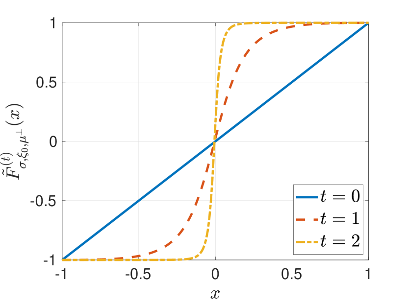
Figure 16: $\tilde{F}_{\sigma,\xi_{0},\bm{\mu}^{\bot}}^{(t)}(x)$ versus $x$ for $t\in\{0,1,2\}$ when $\sigma=0.5$, $\xi_{0}=0$, $\|\bm{\mu}^{\bot}\|_{2}=1$, $n=10$, and $m=1000$.

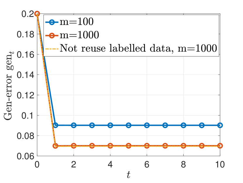
Figure 17: $\mathrm{gen}_{t}$ versus $t$ for $m=100$ and $m=1000$, when $n=10$, $\sigma=0.6$, $d=2$, and $\bm{\mu}=(1,0)$.

As shown in Figure 17, under the same setup as Figure 14(a), when the labelled data $S_{\mathrm{l}}$ are reused in each iteration,

the upper bound for $|\mathrm{gen}_{t}|$ is also a decreasing function of $t$. When $m=1000$, $\mathrm{gen}_{t}$ is almost the same as the gen-error when the labelled data are not reused in the subsequent iterations, which means that for large enough $m/n$, reusing the labelled data does not necessarily help to improve the generalization performance. Moreover, when $m=100$, $\mathrm{gen}_{t}$ is higher than that for $m=1000$, which coincides with the intuition that increasing the number of unlabelled data helps to reduce the generalization error.

Appendix G Proof of Corollary 10

Following similar steps as in Appendix D, we first derive the upper bound for $|\mathrm{gen}_{1}|$.

At $t=1$, from (66) and (94), the expectation $\bm{\mu}_{1}^{\prime\xi_{0},\bm{\mu}^{\bot}}:=\mathbb{E}[\bm{\theta}_{1}^{\prime}|\xi_{0},\bm{\mu}^{\bot}]$ is rewritten as

$$\bm{\mu}_{1}^{\prime\xi_{0},\bm{\mu}^{\bot}} =\frac{n}{n+m}\bm{\theta}_{0}+\frac{1}{n+m}\sum_{i=1}^{m}\mathbb{E}[\operatorname{sgn}(\bar{\bm{\theta}}_{0}^{\top}\mathbf{X}^{\prime}_{j})\mathbf{X}^{\prime}_{j}|\xi_{0},\bm{\mu}^{\bot}]$$

$$=\frac{n}{n+m}\bigg{(}\bigg{(}1+\frac{\sigma}{\sqrt{n}}\xi_{0}\bigg{)}\bm{\mu}+\frac{\sigma}{\sqrt{n}}\bm{\mu}^{\bot}\bigg{)}$$

$$\quad+\frac{m}{n+m}\bigg{(}\bigg{(}1-2\mathrm{Q}\bigg{(}\frac{\alpha}{\sigma}\bigg{)}+\frac{2\sigma\alpha}{\sqrt{2\pi}}\exp\bigg{(}-\frac{\alpha^{2}}{2\sigma^{2}}\bigg{)}\bigg{)}\bm{\mu}+\frac{2\sigma\beta}{\sqrt{2\pi}}\exp\bigg{(}-\frac{\alpha^{2}}{2\sigma^{2}}\bigg{)}\bm{\upsilon}\bigg{)}$$ (226)

$$=\bigg{(}1+\frac{\sqrt{n}\sigma\xi_{0}}{n+m}+\frac{m}{n+m}\bigg{(}-2\mathrm{Q}\bigg{(}\frac{\alpha}{\sigma}\bigg{)}+\frac{2\sigma\alpha}{\sqrt{2\pi}}\exp\bigg{(}-\frac{\alpha^{2}}{2\sigma^{2}}\bigg{)}\bigg{)}\bigg{)}\bm{\mu}$$

$$\quad+\bigg{(}\frac{\sqrt{n}\sigma\|\bm{\mu}^{\bot}\|_{2}}{n+m}+\frac{m}{n+m}\frac{2\sigma\beta}{\sqrt{2\pi}}\exp\bigg{(}-\frac{\alpha^{2}}{2\sigma^{2}}\bigg{)}\bigg{)}\bm{\upsilon}.$$ (227)

Then the correlation between $\bm{\mu}_{1}^{\prime\xi_{0},\bm{\mu}^{\bot}}$ and $\bm{\mu}$ is given by

$$\rho(\bm{\mu}_{1}^{\prime\xi_{0},\bm{\mu}^{\bot}},\bm{\mu})=\tilde{F}_{\sigma,\xi_{0},\bm{\mu}^{\bot}}(\alpha).$$ (228)

The gen-error $\mathrm{gen}_{1}$ is given by

$$\mathrm{gen}_{1} =\frac{1}{n+m}\sum_{i=1}^{n}\mathbb{E}\Big{[}l(\bm{\theta}_{1}^{\prime},(\mathbf{X},Y))-l(\bm{\theta}_{1},(\mathbf{X}_{i},Y_{i}))\Big{]}$$

$$\quad+\frac{1}{n+m}\sum_{i=1}^{m}\mathbb{E}_{\xi_{0},\bm{\mu}^{\bot}}\bigg{[}\mathbb{E}\left[l(\bm{\theta}_{1}^{\prime},(\mathbf{X},Y))-l(\bm{\theta}_{1}^{\prime},(\mathbf{X}^{\prime}_{i},\hat{Y}_{i}^{\prime}))|\xi_{0},\bm{\mu}^{\bot}\right]\bigg{]}$$ (229)

$$=\frac{1}{n+m}\sum_{i=1}^{n}\mathbb{E}_{\bm{\theta}_{1}^{\prime}}\Big{[}\mathrm{\Delta h}(P_{\mathbf{Z}}\|P_{\mathbf{Z}_{i}|\bm{\theta}_{1}^{\prime}}|p_{\bm{\theta}_{1}^{\prime}})\Big{]}$$

$$\quad+\frac{1}{n+m}\sum_{i=1}^{m}\sum_{i=1}^{n}\mathbb{E}_{\xi_{0},\bm{\mu}^{\bot}}\mathbb{E}_{\bm{\theta}_{1}^{\prime}|\xi_{0},\bm{\mu}^{\bot}}\bigg{[}\mathrm{\Delta h}(P_{\mathbf{Z}}\|P_{\mathbf{X}_{i}^{\prime},\hat{Y}_{i}^{\prime}|\xi_{0},\bm{\mu}^{\bot}}|p_{\bm{\theta}_{1}^{\prime}})$$

$$\quad+\mathrm{\Delta h}(P_{\mathbf{X}_{i}^{\prime},\hat{Y}_{i}^{\prime}|\xi_{0},\bm{\mu}^{\bot}}\|P_{\mathbf{X}_{i}^{\prime},\hat{Y}_{i}^{\prime}|\xi_{0},\bm{\mu}^{\bot},\bm{\theta}_{1}^{\prime}}|p_{\bm{\theta}_{1}})\bigg{]}.$$ (230)

• Calculate $\mathbb{E}_{\bm{\theta}_{1}^{\prime}}\Big{[}\mathrm{\Delta h}(P_{\mathbf{Z}}\|P_{\mathbf{Z}_{i}|\bm{\theta}_{1}^{\prime}}|p_{\bm{\theta}_{1}^{\prime}})\Big{]}$:

  $$\mathbb{E}_{\bm{\theta}_{1}^{\prime}}\Big{[}\mathrm{\Delta h}(P_{\mathbf{Z}}\|P_{\mathbf{Z}_{i}|\bm{\theta}_{1}^{\prime}}|p_{\bm{\theta}_{1}^{\prime}})\Big{]}$$

  $$=\int Q_{\bm{\theta}_{1}^{\prime}}(\bm{\theta})(P_{\mathbf{Z}}(\mathbf{z})-P_{\mathbf{Z}_{i}|\bm{\theta}_{1}^{\prime}}(\mathbf{z}|\bm{\theta}))\log\frac{1}{p_{\bm{\theta}}(\mathbf{z})}\mathrm{d}\mathbf{z}\mathrm{d}\bm{\theta}$$ (231)

  $$=-\frac{1}{2\sigma^{2}}\int\Big{(}P_{\mathbf{Z}}(\mathbf{x},1)(Q_{\bm{\theta}_{1}^{\prime}}(\bm{\theta})-P_{\bm{\theta}_{1}^{\prime}|\mathbf{Z}_{i}}(\bm{\theta}|\mathbf{x},1))$$

  $$\qquad-P_{\mathbf{Z}}(\mathbf{x},-1)(Q_{\bm{\theta}_{1}^{\prime}}(\bm{\theta})-P_{\bm{\theta}_{1}^{\prime}|\mathbf{Z}_{i}}(\bm{\theta}|\mathbf{x},-1))\Big{)}2\bm{\theta}^{\top}\mathbf{x}~{}\mathrm{d}\mathbf{x}\mathrm{d}\bm{\theta}$$ (232)

  $$=-\frac{1}{\sigma^{2}}\int\Big{(}\frac{\bm{\mu}-\mathbf{x}}{n+m}P_{\mathbf{Z}}(\mathbf{x},1)-\frac{\bm{\mu}+\mathbf{x}}{n+m}P_{\mathbf{Z}}(\mathbf{x},-1)\Big{)}^{\top}\mathbf{x}~{}\mathrm{d}\mathbf{x}$$ (233)

  $$=-\frac{1}{\sigma^{2}}\bigg{(}\frac{\bm{\mu}^{\top}\bm{\mu}-\bm{\mu}^{\top}\bm{\mu}-d\sigma^{2}}{2(n+m)}-\frac{-\bm{\mu}^{\top}\bm{\mu}+\bm{\mu}^{\top}\bm{\mu}+d\sigma^{2}}{2(n+m)}\bigg{)}$$ (234)

  $$=\frac{d}{n+m}.$$ (235)

• Calculate $\mathbb{E}_{\bm{\theta}_{1}^{\prime}|\xi_{0},\bm{\mu}^{\bot}}\big{[}\mathrm{\Delta h}(P_{\mathbf{X}_{i}^{\prime},\hat{Y}_{i}^{\prime}|\xi_{0},\bm{\mu}^{\bot}}\|P_{\mathbf{X}_{i}^{\prime},\hat{Y}_{i}^{\prime}|\xi_{0},\bm{\mu}^{\bot},\bm{\theta}_{1}^{\prime}}|p_{\bm{\theta}_{1}})\big{]}$:

  $$\mathbb{E}_{\bm{\theta}_{1}^{\prime}|\xi_{0},\bm{\mu}^{\bot}}\big{[}\mathrm{\Delta h}(P_{\mathbf{X}_{i}^{\prime},\hat{Y}_{i}^{\prime}|\xi_{0},\bm{\mu}^{\bot}}\|P_{\mathbf{X}_{i}^{\prime},\hat{Y}_{i}^{\prime}|\xi_{0},\bm{\mu}^{\bot},\bm{\theta}_{1}^{\prime}}|p_{\bm{\theta}_{1}})\big{]}$$

  $$=-\frac{1}{\sigma^{2}}\int P_{\mathbf{X}_{i}^{\prime},\hat{Y}_{i}^{\prime}|\xi_{0},\bm{\mu}^{\bot}}(\mathbf{x},y|\xi_{0},\bm{\mu}^{\bot})\big{(}Q_{\bm{\theta}_{1}^{\prime}|\xi_{0},\bm{\mu}^{\bot}}(\bm{\theta}|\xi_{0},\bm{\mu}^{\bot})$$

  $$\qquad\qquad-P_{\bm{\theta}_{1}^{\prime}|\mathbf{X}_{i}^{\prime},\hat{Y}_{i}^{\prime},\xi_{0},\bm{\mu}^{\bot}}(\bm{\theta}|\mathbf{x},y,\xi_{0},\bm{\mu}^{\bot})\big{)}(y\bm{\theta}^{\top}\mathbf{x})\mathrm{d}\mathbf{x}\mathrm{d}y\mathrm{d}\bm{\theta}$$ (236)

  $$=-\frac{1}{\sigma^{2}}\int P_{\mathbf{X}_{i}^{\prime},\hat{Y}_{i}^{\prime}|\xi_{0},\bm{\mu}^{\bot}}(\mathbf{x},y|\xi_{0},\bm{\mu}^{\bot})\bigg{(}\frac{\bm{\mu}_{1}^{\xi_{0},\bm{\mu}^{\bot}}-y\mathbf{x}}{n+m}\bigg{)}^{\top}(y\mathbf{x})\mathrm{d}\mathbf{x}\mathrm{d}y$$ (237)

  $$=\frac{1}{(n+m)\sigma^{2}}\Big{(}\mathbb{E}[\mathbf{X}_{i}^{\prime\top}\mathbf{X}_{i}^{\prime}|\xi_{0},\bm{\mu}^{\bot}]-(\bm{\mu}_{1}^{\xi_{0},\bm{\mu}^{\bot}})^{\top}\bm{\mu}_{1}^{\xi_{0},\bm{\mu}^{\bot}}\Big{)}$$ (238)

  $$=\frac{d\sigma^{2}+\bm{\mu}^{\top}\bm{\mu}-(\bm{\mu}_{1}^{\xi_{0},\bm{\mu}^{\bot}})^{\top}\bm{\mu}_{1}^{\xi_{0},\bm{\mu}^{\bot}}}{(n+m)\sigma^{2}}$$ (239)

  $$=\frac{d\sigma^{2}+1-J_{\sigma}^{2}(\alpha)-K_{\sigma}^{2}(\alpha)}{(n+m)\sigma^{2}}.$$ (240)

• Calculate $\mathbb{E}_{\bm{\theta}_{1}^{\prime}|\xi_{0},\bm{\mu}^{\bot}}[\mathrm{\Delta h}(P_{\mathbf{Z}}\|P_{\mathbf{X}_{i}^{\prime},\hat{Y}_{i}^{\prime}|\xi_{0},\bm{\mu}^{\bot}}|p_{\bm{\theta}_{1}^{\prime}})]$: Since given any fixed $\bm{\theta}_{1}$, $p_{\bm{\theta}_{1}^{\prime}}(\mathbf{x}|\cdot)$ is a Gaussian distribution, for any $y\in\{\pm 1\}$, we have

  $$\frac{1}{2}\int P_{\bm{\theta}_{1}^{\prime}|\xi_{0},\bm{\mu}^{\bot}}(\bm{\theta})\big{(}P_{\mathbf{X}|Y}(\mathbf{x}|\mathbf{y})-P_{\mathbf{X}_{i}^{\prime}|\hat{Y}_{i}^{\prime}}(\mathbf{x}|y)\big{)}\log\frac{1}{p_{\bm{\theta}}(\mathbf{x}|y)}\mathrm{d}\mathbf{x}\mathrm{d}\bm{\theta}$$

  $$=\frac{1}{4\sigma^{2}}\int P_{\bm{\theta}_{1}^{\prime}|\xi_{0},\bm{\mu}^{\bot}}(\bm{\theta})\big{(}P_{\mathbf{X}|Y}(\mathbf{x}|y)-P_{\mathbf{X}_{i}^{\prime}|\hat{Y}_{i}^{\prime}}(\mathbf{x}|y)\big{)}\big{(}\mathbf{x}^{\top}\mathbf{x}-2y\bm{\theta}^{\top}\mathbf{x}+\bm{\theta}^{\top}\bm{\theta}\big{)}\mathrm{d}\mathbf{x}\mathrm{d}\bm{\theta}$$ (241)

  $$=-\frac{1}{2\sigma^{2}}\int P_{\bm{\theta}_{1}^{\prime}|\xi_{0},\bm{\mu}^{\bot}}(\bm{\theta})\bigg{(}\frac{1}{2}P_{\mathbf{X}|Y}(\mathbf{x}|y)-\frac{1}{2}P_{\mathbf{X}_{i}^{\prime}|\hat{Y}_{i}^{\prime}}(\mathbf{x}|y)\bigg{)}\big{(}y\bm{\theta}^{\top}\mathbf{x}\big{)}\mathrm{d}\mathbf{x}\mathrm{d}\bm{\theta}$$ (242)

  $$=-\frac{1}{2\sigma^{2}}(\bm{\mu}_{1}^{\prime\xi_{0},\bm{\mu}^{\bot}})^{\top}\big{(}\bm{\mu}-\bm{\mu}_{1}^{\xi_{0},\bm{\mu}^{\bot}}\big{)}$$ (243)

  $$=\frac{m(J_{\sigma}^{2}(\alpha)+K_{\sigma}^{2}(\alpha))-(m-n)J_{\sigma}(\alpha)-n}{2\sigma^{2}(n+m)},$$ (244)

  and then

  $$\mathbb{E}_{\bm{\theta}_{1}^{\prime}|\xi_{0},\bm{\mu}^{\bot}}[\mathrm{\Delta h}(P_{\mathbf{Z}}\|P_{\mathbf{X}_{i}^{\prime},\hat{Y}_{i}^{\prime}|\xi_{0},\bm{\mu}^{\bot}}|p_{\bm{\theta}_{1}^{\prime}})]=\frac{m(J_{\sigma}^{2}(\alpha)+K_{\sigma}^{2}(\alpha))-(m-n)J_{\sigma}(\alpha)-n}{\sigma^{2}(n+m)}.$$ (245)

Therefore, the gen-error at $t=1$ can be exactly characterized as follows

$$\mathrm{gen}_{1} =\mathbb{E}_{\xi_{0},\bm{\mu}^{\bot}}\bigg{[}\frac{nd}{(n+m)^{2}\sigma^{2}}$$

$$\qquad+\frac{m}{n+m}\frac{d\sigma^{2}+1-J_{\sigma}^{2}(\alpha)-K_{\sigma}^{2}(\alpha)+m(J_{\sigma}^{2}(\alpha)+K_{\sigma}^{2}(\alpha))-(m-n)J_{\sigma}(\alpha)-n}{(n+m)\sigma^{2}}\bigg{]}$$ (246)

$$=\mathbb{E}_{\xi_{0},\bm{\mu}^{\bot}}\bigg{[}\frac{m(m-1)(J_{\sigma}^{2}(\alpha)+K_{\sigma}^{2}(\alpha))-m(m-n)J_{\sigma}(\alpha)-nm+m(1+d\sigma^{2})+nd}{(n+m)^{2}\sigma^{2}}\bigg{]}.$$ (247)

For $t\geq 2$, similar to the derivation in Appendix C, by iteratively implementing the calculation, we only need to replace $\alpha$ with the correlation evolution function $\tilde{F}_{\sigma,\xi_{0},\bm{\mu}^{\bot}}(\cdot)$ (cf. (224)) and then the gen-error for any $t\geq 1$ is characterized as follows. For almost all sample paths, there exists a vanishing sequence $\epsilon_{m}$ ($\epsilon_{m}\to 0$ as $m\to\infty$) , such that

$$\mathrm{gen}_{t}=\mathbb{E}_{\xi_{0},\bm{\mu}^{\bot}}\bigg{[} \frac{m(m-1)(J_{\sigma}^{2}(\tilde{F}_{\sigma,\xi_{0},\bm{\mu}^{\bot}}(\alpha))+K_{\sigma}^{2}(\tilde{F}_{\sigma,\xi_{0},\bm{\mu}^{\bot}}(\alpha)))}{(n+m)^{2}\sigma^{2}}$$

$$+\frac{-m(m-n)J_{\sigma}(\tilde{F}_{\sigma,\xi_{0},\bm{\mu}^{\bot}}(\alpha))-nm}{(n+m)^{2}\sigma^{2}}\bigg{]}+\epsilon_{m}^{\prime},$$ (248)

where $\epsilon_{m}^{\prime}=\epsilon_{m}+\frac{m(1+d\sigma^{2})+nd}{(n+m)^{2}\sigma^{2}}\to 0$ as $m\to\infty$ and $\alpha$ stands for $\alpha(\xi_{0},\bm{\mu}^{\bot})$.

The proof of Corollary 10 is thus completed.

Appendix H Proof of Theorem 4

Theorem 4 can be proved similarly from the proof of Theorem 7. For simplicity, in the following proofs, we abbrviate $\mathrm{gen}_{t}(P_{\mathbf{Z}},P_{\mathbf{X}},\{P_{\bm{\theta}_{k}|S_{\mathrm{l}},S_{\mathrm{u}}}\}_{k=0}^{t},\{f_{\bm{\theta}_{k}}\}_{k=0}^{t-1})$ as $\mathrm{gen}_{t}$. With $\ell_{2}$-regularization, the algorithm operates in the following steps. Let $\lambda\in\mathbb{R}_{+}$ be the regularization parameter.

• Step 1: Initial round $t=0$ with $S_{\mathrm{l}}$: By minimizing the regularized empirical risk of labelled dataset $S_{\mathrm{l}}$

  $$L_{S_{\mathrm{l}}}^{\mathrm{reg}}(\bm{\theta}) =\frac{1}{n}\sum_{i=1}^{n}l(\bm{\theta},(\mathbf{X}_{i},Y_{i}))+\frac{\lambda}{2}\|\bm{\theta}\|_{2}^{2}\overset{\mathrm{c}}{=}\frac{1}{2\sigma^{2}n}\sum_{i=1}^{n}(\mathbf{X}_{i}-Y_{i}\bm{\theta})^{\top}(\mathbf{X}_{i}-Y_{i}\bm{\theta})+\frac{\lambda}{2}\|\bm{\theta}\|_{2}^{2},$$ (249)

  where $\stackrel{{\scriptstyle\mathrm{c}}}{{=}}$ means that both sides differ by a constant independent of $\bm{\theta}$, we obtain the minimizer

  $$\bm{\theta}_{0}^{\mathrm{reg}} =\operatorname*{arg\,min}_{\bm{\theta}\in\Theta}L_{S_{\mathrm{l}}}(\bm{\theta})=\frac{1}{n}\sum_{i=1}^{n}\frac{Y_{i}\mathbf{X}_{i}}{1+\sigma^{2}\lambda}$$

  $$=\frac{\bm{\theta}_{0}}{1+\sigma^{2}\lambda}\sim\mathcal{N}\bigg{(}\frac{\bm{\mu}}{1+\sigma^{2}\lambda},\frac{\sigma^{2}}{n(1+\sigma^{2}\lambda)^{2}}\mathbf{I}_{d}\bigg{)}.$$ (250)

• Step 2: Pseudo-label data in $S_{\mathrm{u}}$: At each iteration $t\in[1:\tau]$, for any $i\in\mathcal{I}_{t}$, we use $\bm{\theta}_{t-1}^{\mathrm{reg}}$ to assign a pseudo-label for $\mathbf{X}_{i}^{\prime}$, that is, $\hat{Y}_{i}^{\prime}=f_{\bm{\theta}_{t-1}^{\mathrm{reg}}}(\mathbf{X}_{i}^{\prime})=\operatorname{sgn}(\mathbf{X}_{i}^{\prime\top}\bm{\theta}_{t-1}^{\mathrm{reg}})$.

• Step 3: Refine the model: We then use the pseudo-labelled dataset $\hat{S}_{\mathrm{u},t}$ to train the new model. By minimizing the empirical risk of $\hat{S}_{\mathrm{u},t}$

  $$L_{\hat{S}_{\mathrm{u},t}}(\bm{\theta}) =\frac{1}{m}\sum_{i\in\mathcal{I}_{t}}l(\bm{\theta},(\mathbf{X}^{\prime}_{i},\hat{Y}_{i}^{\prime}))+\frac{\lambda}{2m}\|\bm{\theta}\|_{2}^{2}$$

  $$\overset{\mathrm{c}}{=}\frac{1}{2\sigma^{2}m}\sum_{i\in\mathcal{I}_{t}}(\mathbf{X}^{\prime}_{i}-\hat{Y}_{i}^{\prime}\bm{\theta})^{\top}(\mathbf{X}^{\prime}_{i}-\hat{Y}_{i}^{\prime}\bm{\theta})+\frac{\lambda}{2}\|\bm{\theta}\|_{2}^{2},$$ (251)

  we obtain the new model parameter

  $$\bm{\theta}_{t}^{\mathrm{reg}} =\frac{1}{m}\sum_{i\in\mathcal{I}_{t}}\frac{\hat{Y}_{i}^{\prime}\mathbf{X}^{\prime}_{i}}{1+\sigma^{2}\lambda}=\frac{1}{m}\sum_{i\in\mathcal{I}_{t}}\frac{\operatorname{sgn}(\mathbf{X}_{i}^{\prime\top}\bm{\theta}_{t-1}^{\mathrm{reg}})\mathbf{X}^{\prime}_{i}}{1+\sigma^{2}\lambda}.$$ (252)

  If $t<\tau$, go back to Step 2.

1. Characterization of $|\mathrm{gen}_{1}|$:

   From (250), we still have $\rho(\bm{\theta}_{0}^{\mathrm{reg}},\bm{\mu})=\alpha(\xi_{0},\bm{\mu}^{\bot})$ and

   $$\bar{\bm{\theta}}_{0}^{\mathrm{reg}}:=\frac{\bm{\theta}_{0}^{\mathrm{reg}}}{\|\bm{\theta}_{0}^{\mathrm{reg}}\|_{2}^{2}}=\alpha\bm{\mu}+\beta\bm{\upsilon}=\bar{\bm{\theta}}_{0}.$$ (253)

   From (253), we can rewrite (252) as follows

   $$\bm{\theta}_{1}^{\mathrm{reg}} =\frac{1}{m}\sum_{i=1}^{m}\frac{\operatorname{sgn}(\mathbf{X}_{i}^{\prime\top}\bar{\bm{\theta}}_{1}^{\mathrm{reg}})\mathbf{X}^{\prime}_{i}}{1+\sigma^{2}\lambda}=\frac{1}{m}\sum_{i=1}^{m}\frac{\operatorname{sgn}(\mathbf{X}_{i}^{\prime\top}\bar{\bm{\theta}}_{0})\mathbf{X}^{\prime}_{i}}{1+\sigma^{2}\lambda}=\frac{\bm{\theta}_{1}}{1+\sigma^{2}\lambda}.$$ (254)

   Thus, the expectation of $\bm{\theta}_{1}^{\mathrm{reg}}$ conditioned on $(\xi_{0},\bm{\mu}^{\bot})$ is given by

   $$\bm{\mu}_{1}^{\mathrm{reg}|\xi_{0},\bm{\mu}^{\bot}}:=\frac{1}{1+\sigma^{2}\lambda}\mathbb{E}[\operatorname{sgn}(\mathbf{X}_{j}^{\prime\top}\bm{\theta}_{0}^{\mathrm{reg}})\mathbf{X}^{\prime}_{j}|\xi_{0},\bm{\mu}^{\bot}]$$ (255)

   $$=\frac{1}{1+\sigma^{2}\lambda}\bm{\mu}_{1}^{\xi_{0},\bm{\mu}^{\bot}}$$ (256)

   $$=\frac{1}{1+\sigma^{2}\lambda}\bigg{(}\bigg{(}1-2\mathrm{Q}\bigg{(}\frac{\alpha}{\sigma}\bigg{)}+\frac{2\sigma\alpha}{\sqrt{2\pi}}\exp\bigg{(}-\frac{\alpha^{2}}{2\sigma^{2}}\bigg{)}\bigg{)}\bm{\mu}+\frac{2\sigma\beta}{\sqrt{2\pi}}\exp\bigg{(}-\frac{\alpha^{2}}{2\sigma^{2}}\bigg{)}\bm{\upsilon}\bigg{)}$$ (257)

   $$=\frac{J_{\sigma}(\alpha)\bm{\mu}+K_{\sigma}(\alpha)\bm{\upsilon}}{1+\sigma^{2}\lambda}.$$ (258)

   Recall $\mathrm{gen}_{1}$ given in (95). In the case with regularization, the gen-error $\mathrm{gen}_{1}^{\mathrm{reg}}$ has the same definition as $\mathrm{gen}_{1}$. To derive $\mathrm{gen}_{1}^{\mathrm{reg}}$, we need to calculate the following two terms.

   • Calculate $\mathbb{E}_{\bm{\theta}_{1}^{\mathrm{reg}}|\xi_{0},\bm{\mu}^{\bot}}\big{[}\mathrm{\Delta h}(P_{\mathbf{X}_{i}^{\prime},\hat{Y}_{i}^{\prime}|\xi_{0},\bm{\mu}^{\bot}}\|P_{\mathbf{X}_{i}^{\prime},\hat{Y}_{i}^{\prime}|\xi_{0},\bm{\mu}^{\bot},\bm{\theta}_{1}^{\mathrm{reg}}}|p_{\bm{\theta}_{1}^{\mathrm{reg}}})\big{]}$:

     $$\mathbb{E}_{\bm{\theta}_{1}^{\mathrm{reg}}|\xi_{0},\bm{\mu}^{\bot}}\big{[}\mathrm{\Delta h}(P_{\mathbf{X}_{i}^{\prime},\hat{Y}_{i}^{\prime}|\xi_{0},\bm{\mu}^{\bot}}\|P_{\mathbf{X}_{i}^{\prime},\hat{Y}_{i}^{\prime}|\xi_{0},\bm{\mu}^{\bot},\bm{\theta}_{1}^{\mathrm{reg}}}|p_{\bm{\theta}_{1}^{\mathrm{reg}}})\big{]}$$

     $$=\frac{1}{2\sigma^{2}}\int Q_{\bm{\theta}_{1}^{\mathrm{reg}}|\xi_{0},\bm{\mu}^{\bot}}(\bm{\theta}|\xi_{0},\bm{\mu}^{\bot})\big{(}P_{\mathbf{X}_{i}^{\prime},\hat{Y}_{i}^{\prime}|\xi_{0},\bm{\mu}^{\bot}}(\mathbf{x},y|\xi_{0},\bm{\mu}^{\bot})$$

     $$\qquad\qquad-P_{\mathbf{X}_{i}^{\prime},\hat{Y}_{i}^{\prime}|\xi_{0},\bm{\mu}^{\bot},\bm{\theta}_{1}^{\mathrm{reg}}}(\mathbf{x},y|\xi_{0},\bm{\mu}^{\bot},\bm{\theta})\big{)}(\mathbf{x}^{\top}\mathbf{x}-2y\bm{\theta}^{\top}\mathbf{x}+\bm{\theta}^{\top}\bm{\theta})\mathrm{d}\mathbf{x}\mathrm{d}y\mathrm{d}\bm{\theta}$$ (259)

     $$=-\frac{1}{\sigma^{2}}\int P_{\mathbf{X}_{i}^{\prime},\hat{Y}_{i}^{\prime}|\xi_{0},\bm{\mu}^{\bot}}(\mathbf{x},y|\xi_{0},\bm{\mu}^{\bot})\big{(}Q_{\bm{\theta}_{1}^{\mathrm{reg}}|\xi_{0},\bm{\mu}^{\bot}}(\bm{\theta}|\xi_{0},\bm{\mu}^{\bot})$$

     $$\qquad\qquad-P_{\bm{\theta}_{1}^{\mathrm{reg}}|\mathbf{X}_{i}^{\prime},\hat{Y}_{i}^{\prime},\xi_{0},\bm{\mu}^{\bot}}(\bm{\theta}|\mathbf{x},y,\xi_{0},\bm{\mu}^{\bot})\big{)}(y\bm{\theta}^{\top}\mathbf{x})\mathrm{d}\mathbf{x}\mathrm{d}y\mathrm{d}\bm{\theta}$$ (260)

     $$=-\frac{1}{\sigma^{2}}\int P_{\mathbf{X}_{i}^{\prime},\hat{Y}_{i}^{\prime}|\xi_{0},\bm{\mu}^{\bot}}(\mathbf{x},y|\xi_{0},\bm{\mu}^{\bot})\bigg{(}\frac{\bm{\mu}_{1}^{\xi_{0},\bm{\mu}^{\bot}}-y\mathbf{x}}{m(1+\sigma^{2}\lambda)}\bigg{)}^{\top}(y\mathbf{x})\mathrm{d}\mathbf{x}\mathrm{d}y$$ (261)

     $$=\frac{1}{m\sigma^{2}(1+\sigma^{2}\lambda)}\Big{(}\mathbb{E}[\mathbf{X}_{i}^{\prime\top}\mathbf{X}_{i}^{\prime}|\xi_{0},\bm{\mu}^{\bot}]-(\bm{\mu}_{1}^{\xi_{0},\bm{\mu}^{\bot}})^{\top}\bm{\mu}_{1}^{\xi_{0},\bm{\mu}^{\bot}}\Big{)}$$ (262)

     $$=\frac{d\sigma^{2}+\bm{\mu}^{\top}\bm{\mu}-(\bm{\mu}_{1}^{\xi_{0},\bm{\mu}^{\bot}})^{\top}\bm{\mu}_{1}^{\xi_{0},\bm{\mu}^{\bot}}}{m\sigma^{2}(1+\sigma^{2}\lambda)}$$ (263)

     $$=\frac{d\sigma^{2}+1-J_{\sigma}^{2}(\alpha)-K_{\sigma}^{2}(\alpha)}{m\sigma^{2}(1+\sigma^{2}\lambda)}.$$ (264)

   • Calculate $\mathbb{E}_{\bm{\theta}_{1}^{\mathrm{reg}}|\xi_{0},\bm{\mu}^{\bot}}\big{[}h(P_{\mathbf{Z}},p_{\bm{\theta}_{1}^{\mathrm{reg}}})-h(P_{\mathbf{X}_{i}^{\prime},\hat{Y}_{i}^{\prime}|\xi_{0},\bm{\mu}^{\bot}},p_{\bm{\theta}_{1}^{\mathrm{reg}}})\big{]}$: Given any $(\xi_{0},\bm{\mu}^{\bot})$, in the following, we drop the condition on $\xi_{0},\bm{\mu}^{\bot}$ for notational simplicity. Since given $\bm{\theta}_{1}$, $p_{\bm{\theta}_{1}}(\mathbf{x}|\cdot)$ is a Gaussian distribution, for any $y\in\{\pm 1\}$, we have

     $$\frac{1}{2}\int P_{\bm{\theta}_{1}^{\mathrm{reg}}|\xi_{0},\bm{\mu}^{\bot}}(\bm{\theta})\big{(}P_{\mathbf{X}|Y}(\mathbf{x}|\mathbf{y})-P_{\mathbf{X}_{i}^{\prime}|\hat{Y}_{i}^{\prime}}(\mathbf{x}|y)\big{)}\log\frac{1}{p_{\bm{\theta}}(\mathbf{x}|y)}\mathrm{d}\mathbf{x}\mathrm{d}\bm{\theta}$$

     $$=-\frac{1}{2\sigma^{2}}\int P_{\bm{\theta}_{1}^{\mathrm{reg}}|\xi_{0},\bm{\mu}^{\bot}}(\bm{\theta})\bigg{(}\frac{1}{2}P_{\mathbf{X}|Y}(\mathbf{x}|y)-\frac{1}{2}P_{\mathbf{X}_{i}^{\prime}|\hat{Y}_{i}^{\prime}}(\mathbf{x}|y)\bigg{)}\big{(}y\bm{\theta}^{\top}\mathbf{x}\big{)}\mathrm{d}\mathbf{x}\mathrm{d}\bm{\theta}$$ (265)

     $$=-\frac{1}{2\sigma^{2}}(\bm{\mu}_{1}^{\mathrm{reg}|\xi_{0},\bm{\mu}^{\bot}})^{\top}\big{(}\bm{\mu}-\bm{\mu}_{1}^{\xi_{0},\bm{\mu}^{\bot}}\big{)}$$ (266)

     $$=\frac{J_{\sigma}^{2}(\alpha)+K_{\sigma}^{2}(\alpha)-J_{\sigma}(\alpha)}{2\sigma^{2}(1+\sigma^{2}\lambda)}.$$ (267)

     Thus, we have

     $$\mathbb{E}_{\bm{\theta}_{1}|\xi_{0},\bm{\mu}^{\bot}}[\mathrm{\Delta h}(P_{\mathbf{Z}}\|P_{\mathbf{X}_{i}^{\prime},\hat{Y}_{i}^{\prime}|\xi_{0},\bm{\mu}^{\bot}}|p_{\bm{\theta}_{1}})]=\frac{J_{\sigma}^{2}(\alpha)+K_{\sigma}^{2}(\alpha)-J_{\sigma}(\alpha)}{\sigma^{2}(1+\sigma^{2}\lambda)}.$$ (268)

   Finally, the gen-error at $t=1$ can be characterized as follows:

   $$\mathrm{gen}_{1}^{\mathrm{reg}}=\mathbb{E}_{\xi_{0},\bm{\mu}^{\bot}}\bigg{[}\frac{J_{\sigma}^{2}(\alpha)+K_{\sigma}^{2}(\alpha)-J_{\sigma}(\alpha)}{\sigma^{2}(1+\sigma^{2}\lambda)}+\frac{d\sigma^{2}+1-J_{\sigma}^{2}(\alpha)-K_{\sigma}^{2}(\alpha)}{m\sigma^{2}(1+\sigma^{2}\lambda)}\bigg{]}=\frac{\mathrm{gen}_{1}}{1+\sigma^{2}\lambda},$$ (269)

   where $\alpha$ stands for $\alpha(\xi_{0},\bm{\mu}^{\bot})$.

2. Iteration $t\in[2:\tau]$: Since $\bm{\theta}_{t}^{\mathrm{reg}}=\frac{\bm{\theta}_{t}}{1+\sigma^{2}\lambda}$, by iteratively applying the same techniques in iteration $t=1$ and in Appendix C, the gen-error at any $t\in[2:\tau]$ can be characterized as follows

   $$\mathrm{gen}_{t}^{\mathrm{reg}}=\frac{\mathrm{gen}_{t}}{1+\sigma^{2}\lambda}.$$ (270)

Theorem 4 is thus proved.

References

- Akaho and Kappen (2000) Shotaro Akaho and Hilbert J Kappen. Nonmonotonic generalization bias of Gaussian mixture models. Neural Computation, 12(6):1411–1427, 2000.
- Aminian et al. (2021) Gholamali Aminian, Yuheng Bu, Laura Toni, Miguel Rodrigues, and Gregory Wornell. An exact characterization of the generalization error for the Gibbs algorithm. Advances in Neural Information Processing Systems, 34, 2021.
- Aminian et al. (2022) Gholamali Aminian, Mahed Abroshan, Mohammad Mahdi Khalili, Laura Toni, and Miguel Rodrigues. An information-theoretical approach to semi-supervised learning under covariate-shift. In Proceedings of The 25th International Conference on Artificial Intelligence and Statistics, volume 151, pages 7433–7449. PMLR, 28–30 Mar 2022.
- Anzai (2012) Yuichiro Anzai. Pattern Recognition and Machine Learning. Elsevier, 2012.
- Arazo et al. (2020) Eric Arazo, Diego Ortego, Paul Albert, Noel E O’Connor, and Kevin McGuinness. Pseudo-labeling and confirmation bias in deep semi-supervised learning. In 2020 International Joint Conference on Neural Networks (IJCNN), pages 1–8. IEEE, 2020.
- Boucheron et al. (2005) Stéphane Boucheron, Olivier Bousquet, and Gábor Lugosi. Theory of classification: A survey of some recent advances. ESAIM: Probability and Statistics, 9:323–375, 2005.
- Boucheron et al. (2013) Stéphane Boucheron, Gábor Lugosi, and Pascal Massart. Concentration Inequalities: A Nonasymptotic Theory of Independence. Oxford University Press, 2013.
- Bousquet and Elisseeff (2002) Olivier Bousquet and André Elisseeff. Stability and generalization. The Journal of Machine Learning Research, 2:499–526, 2002.
- Bu et al. (2020) Yuheng Bu, Shaofeng Zou, and Venugopal V Veeravalli. Tightening mutual information based bounds on generalization error. IEEE Journal on Selected Areas in Information Theory, 1(1):121–130, 2020.
- Bu et al. (2022) Yuheng Bu, Gholamali Aminian, Laura Toni, Gregory W. Wornell, and Miguel Rodrigues. Characterizing and understanding the generalization error of transfer learning with Gibbs algorithm. In Proceedings of The 25th International Conference on Artificial Intelligence and Statistics, volume 151, pages 8673–8699. PMLR, 28–30 Mar 2022.
- Cao et al. (2019) Kaidi Cao, Colin Wei, Adrien Gaidon, Nikos Arechiga, and Tengyu Ma. Learning imbalanced datasets with label-distribution-aware margin loss. In Proceedings of the 33rd International Conference on Neural Information Processing Systems, pages 1567–1578, 2019.
- Carmon et al. (2019) Yair Carmon, Aditi Raghunathan, Ludwig Schmidt, Percy Liang, and John C Duchi. Unlabeled data improves adversarial robustness. In Proceedings of the 33rd International Conference on Neural Information Processing Systems, pages 11192–11203, 2019.
- Castelli and Cover (1996) Vittorio Castelli and Thomas M Cover. The relative value of labeled and unlabeled samples in pattern recognition with an unknown mixing parameter. IEEE Transactions on Information Theory, 42(6):2102–2117, 1996.
- Chapelle et al. (2006) Olivier Chapelle, Bernhard Schölkopf, and Alexander Zien, editors. Semi-Supervised Learning. The MIT Press, 2006.
- Chawla and Karakoulas (2005) Nitesh V Chawla and Grigoris Karakoulas. Learning from labeled and unlabeled data: An empirical study across techniques and domains. Journal of Artificial Intelligence Research, 23:331–366, 2005.
- Dupre et al. (2019) Robert Dupre, Jiri Fajtl, Vasileios Argyriou, and Paolo Remagnino. Improving dataset volumes and model accuracy with semi-supervised iterative self-learning. IEEE Transactions on Image Processing, 29:4337–4348, 2019.
- Esposito et al. (2021) Amedeo Roberto Esposito, Michael Gastpar, and Ibrahim Issa. Generalization error bounds via Rényi-, -divergences and maximal leakage. IEEE Transactions on Information Theory, 67(8):4986–5004, 2021.
- Goodfellow et al. (2016) Ian Goodfellow, Yoshua Bengio, and Aaron Courville. Deep Learning. MIT press, 2016.
- Haghifam et al. (2020) Mahdi Haghifam, Jeffrey Negrea, Ashish Khisti, Daniel M Roy, and Gintare Karolina Dziugaite. Sharpened generalization bounds based on conditional mutual information and an application to noisy, iterative algorithms. Advances in Neural Information Processing Systems, 33:9925–9935, 2020.
- He et al. (2016) Kaiming He, Xiangyu Zhang, Shaoqing Ren, and Jian Sun. Deep residual learning for image recognition. In Proceedings of the IEEE Conference on Computer Vision and Pattern Recognition, pages 770–778, 2016.
- Jose and Simeone (2021) Sharu Theresa Jose and Osvaldo Simeone. Information-theoretic bounds on transfer generalization gap based on Jensen–Shannon divergence. In 2021 29th European Signal Processing Conference (EUSIPCO), pages 1461–1465. IEEE, 2021.
- Kawaguchi et al. (2017) Kenji Kawaguchi, Leslie Pack Kaelbling, and Yoshua Bengio. Generalization in deep learning. arXiv preprint arXiv:1710.05468, 2017.
- Krizhevsky (2009) Alex Krizhevsky. Learning multiple layers of features from tiny images. Master’s thesis, University of Toronto, 2009.
- LeCun et al. (1998) Yann LeCun, Léon Bottou, Yoshua Bengio, and Patrick Haffner. Gradient-based learning applied to document recognition. Proceedings of the IEEE, 86(11):2278–2324, 1998.
- Lee (2013) Dong-Hyun Lee. Pseudo-label: The simple and efficient semi-supervised learning method for deep neural networks. In Workshop on Challenges in Representation Learning, ICML, volume 3, page 896, 2013.
- Li et al. (2019) Jian Li, Yong Liu, Rong Yin, and Weiping Wang. Multi-class learning using unlabeled samples: Theory and algorithm. In International Joint Conference on Artificial Intelligence (IJCAI), pages 2880–2886, 2019.
- Liu and Mukhopadhyay (2018) Qun Liu and Supratik Mukhopadhyay. Unsupervised learning using pretrained CNN and associative memory bank. In 2018 International Joint Conference on Neural Networks (IJCNN), pages 01–08. IEEE, 2018.
- Lopez and Jog (2018) Adrian Tovar Lopez and Varun Jog. Generalization error bounds using Wasserstein distances. In 2018 IEEE Information Theory Workshop (ITW), pages 1–5. IEEE, 2018.
- MacKay (2003) David J. C. MacKay. Information Theory, Inference and Learning Algorithms. Cambridge University Press, 2003.
- Mignacco et al. (2020) Francesca Mignacco, Florent Krzakala, Yue Lu, Pierfrancesco Urbani, and Lenka Zdeborova. The role of regularization in classification of high-dimensional noisy Gaussian mixture. In International Conference on Machine Learning, pages 6874–6883. PMLR, 2020.
- Moody (1992) John Moody. The effective number of parameters: An analysis of generalization and regularization in nonlinear learning systems. Advances in Neural Information Processing Systems, 4, 1992.
- Muthukumar et al. (2021) Vidya Muthukumar, Adhyyan Narang, Vignesh Subramanian, Mikhail Belkin, Daniel Hsu, and Anant Sahai. Classification vs regression in overparameterized regimes: Does the loss function matter? Journal of Machine Learning Research, 22(222):1–69, 2021.
- Negrea et al. (2019) Jeffrey Negrea, Mahdi Haghifam, Gintare Karolina Dziugaite, Ashish Khisti, and Daniel M Roy. Information-theoretic generalization bounds for SGLD via data-dependent estimates. In Advances in Neural Information Processing Systems, pages 11013–11023, 2019.
- Oymak and Gülcü (2021) Samet Oymak and Talha Cihad Gülcü. A theoretical characterization of semi-supervised learning with self-training for Gaussian mixture models. In International Conference on Artificial Intelligence and Statistics, pages 3601–3609. PMLR, 2021.
- Pensia et al. (2018) Ankit Pensia, Varun Jog, and Po-Ling Loh. Generalization error bounds for noisy, iterative algorithms. In 2018 IEEE International Symposium on Information Theory (ISIT), pages 546–550. IEEE, 2018.
- Russo and Zou (2016) Daniel Russo and James Zou. Controlling bias in adaptive data analysis using information theory. In Arthur Gretton and Christian C. Robert, editors, Proceedings of the 19th International Conference on Artificial Intelligence and Statistics, volume 51, pages 1232–1240, Cadiz, Spain, 09–11 May 2016. PMLR.
- Singh et al. (2008) Aarti Singh, Robert Nowak, and Jerry Zhu. Unlabeled data: Now it helps, now it doesn’t. Advances in Neural Information Processing Systems, 21:1513–1520, 2008.
- Steinke and Zakynthinou (2020) Thomas Steinke and Lydia Zakynthinou. Reasoning About Generalization via Conditional Mutual Information. In Jacob Abernethy and Shivani Agarwal, editors, Proceedings of Thirty Third Conference on Learning Theory, volume 125, pages 3437–3452. PMLR, 09–12 Jul 2020.
- Triguero et al. (2015) Isaac Triguero, Salvador García, and Francisco Herrera. Self-labeled techniques for semi-supervised learning: taxonomy, software and empirical study. Knowledge and Information Systems, 42(2):245–284, 2015.
- Van Engelen and Hoos (2020) Jesper E Van Engelen and Holger H Hoos. A survey on semi-supervised learning. Machine Learning, 109(2):373–440, 2020.
- Vapnik (2000) Vladimir Vapnik. The Nature of Statistical Learning Theory. Springer, 2000.
- Vershynin (2018) Roman Vershynin. High-Dimensional Probability: An Introduction with Applications in Data Science. Cambridge Series in Statistical and Probabilistic Mathematics. Cambridge University Press, 2018.
- Wang and Thrampoulidis (2022) Ke Wang and Christos Thrampoulidis. Binary classification of gaussian mixtures: Abundance of support vectors, benign overfitting, and regularization. SIAM Journal on Mathematics of Data Science, 4(1):260–284, 2022.
- Watanabe and Watanabe (2006) Kazuho Watanabe and Sumio Watanabe. Stochastic complexities of Gaussian mixtures in variational Bayesian approximation. The Journal of Machine Learning Research, 7:625–644, 2006.
- Wu et al. (2020) Xuetong Wu, Jonathan H Manton, Uwe Aickelin, and Jingge Zhu. Information-theoretic analysis for transfer learning. In 2020 IEEE International Symposium on Information Theory (ISIT), pages 2819–2824. IEEE, 2020.
- Xu and Raginsky (2017) Aolin Xu and Maxim Raginsky. Information-theoretic analysis of generalization capability of learning algorithms. In Advances in Neural Information Processing Systems, pages 2524–2533, 2017.
- Zhu (2020) Jingge Zhu. Semi-supervised learning: the case when unlabeled data is equally useful. In Proceedings of the 36th Conference on Uncertainty in Artificial Intelligence (UAI), volume 124, pages 709–718. PMLR, 03–06 Aug 2020.
- Zhu and Goldberg (2009) Xiaojin Zhu and Andrew B Goldberg. Introduction to semi-supervised learning. Synthesis Lectures on Artificial Intelligence and Machine Learning, 3(1):1–130, 2009.
- Zhu (2008) Xiaojin Jerry Zhu. Semi-supervised learning literature survey. Technical report, University of Wisconsin-Madison Department of Computer Sciences, 2008.