EAST discharge prediction without integrating simulation results

Abstract

In this work, a purely data-driven discharge prediction model was developed and tested without integrating any data or results from simulations. The model was developed based on the experimental data from the Experimental Advanced Superconducting Tokamak (EAST) campaign 2010-2020 discharges and can predict the actual plasma current $I_{p}$, normalized beta $\beta_{n}$, toroidal beta $\beta_{t}$, beta poloidal $\beta_{p}$, electron density $n_{e}$, store energy $W_{mhd}$, loop voltage $V_{loop}$, elongation at plasma boundary $\kappa$, internal inductance $l_{i}$, q at magnetic axis $q_{0}$, and q at 95% flux surface $q_{95}$. The average similarities of all the selected key diagnostic signals between prediction results and the experimental data are greater than 90%, except for the $V_{loop}$ and $q_{0}$. Before a tokamak experiment, the values of actuator signals are set in the discharge proposal stage, with the model allowing to check the consistency of expected diagnostic signals. The model can give the estimated values of the diagnostic signals to check the reasonableness of the tokamak experimental proposal.

Keywords: discharge prediction, machine learning, tokamak

1 Introduction

The entire prediction of a plasma discharge in a tokamak is a complicated and critical task, which needs to be enhanced beyond the current capabilities of available simulation codes. It is commonly used to check the consistency of the modeled diagnostic signals, assist the experimental data analysis phase, validate theoretical models, control technology R&D, and provide references for the design of an experiment. In the framework of conventional discharge prediction, from a physics point of view, the primary method is "Integrated Modeling" [1] derived from first principles. "Integrated Modeling" involves lots of different physical processes in tokamaks. Its accuracy depends on the completeness and consistency of the tokamak’s physics derivations at the base of the model itself. High-fidelity and fast simulation of the entire tokamak discharge is still an open problem because of the high non-linearity, multi-spatial-temporal scales and multi-physics nature of tokamak plasmas [2].

A neural network based method is an alternative approach for tokamak discharge prediction without integrating complex physical modeling. The method has been adopted in magnetic fusion research to solve a variety of problems, including disruption prediction [3, 4, 5, 6, 7, 8, 9], electron temperature profile estimation from multi-energy SXR diagnostics [10], radiated power estimation [11], filament detection [12], simulation acceleration [13, 14, 15], classifying confinement regimes [16], plasma tomography [17], identification of instabilities [18], estimation of neutral beam effects [19], determination of scaling laws [20, 21] coil current prediction with the heat load pattern [22], equilibrium reconstruction [10, 23, 24, 25, 26, 27], and equilibrium solver [28], control plasma [29, 30, 31, 32, 33, 34], physic-informed machine learning [35]. Additionally, a method mixed neural-network with simulation code for discharge prediction [36] was noted. In that work [36], only the backward (past) observation information was used without considering the forward (future) information. While there are tasks such as disruptions prediction, which must inherently satisfy online causality settings, other tasks like discharge predictive modeling can take advantage of a wider context as far as offline analysis is concerned. In the offline discharge prediction, where backward and forward information is in principle equally important to describe the dynamic of the system. Another limitation of that work is that it allows predicting only a restricted set of signals (i.e., stored energy $W_{mhd}$, loop voltage $V_{loop}$ and electron density $n_{e}$ ). The evolution of a tokamak discharge is a complex process characterized by many global parameters, such as equilibrium and kinetic quantities. The restricted set of quantities namely $W_{mhd}$, $V_{loop}$, $n_{e}$, is still not enough for the predictive modeling of a tokamak discharge. Moreover, the model requires integrating a physical simulation code to estimate the actual $I_{p}$ as an input signal. The total inference time of that model would be long and inefficient. The Tokamak Simulation Code [37, 38] (TSC), as used in that paper to simulate the entire discharge plasma current $I_{p}$ typically takes several hours if multiple models (auxiliary-heating, current-drive, alpha-heating, pellet-injection, etc) are included. In contrast, our model’s typical total inference time is ~1s. In the present work, a new machine learning architecture was designed to consider wider contextual information, predicted eleven key signals of tokamak discharge, and values of all the input signals that can be directly available or given by the machine learning model without integrating any physical simulation code results.

In the present work, we trained the bidirectional long short-term memory (LSTM) models using large-scale data from the EAST tokamak [39, 40, 41] coming from 2010-2020 campaigns. Bidirectional LSTM [42, 43, 44] connects two hidden layers with the information propagating in opposite directions to the same output. The output layer can obtain information from backward and forward states simultaneously with these designations. With the 96 actuator signals (introduce further in table 1) as input, the model is able to reproduce the whole tokamak discharge time evolution of eleven key diagnostic signals, that are actual plasma current $I_{p}$, normalized beta $\beta_{n}$, toroidal beta $\beta_{t}$, beta poloidal $\beta_{p}$, electron density $n_{e}$, store energy $W_{mhd}$, loop voltage $V_{loop}$, elongation at plasma boundary $\kappa$, internal inductance $l_{i}$, q at magnetic axis $q_{0}$, and q at 95% flux surface $q_{95}$.

This paper is organized as follows. First, section 2 details the deep learning model architecture. Then, section 3 describes the data preprocessing and selection criteria. Section 4 shows the model training process. Next, section 5 presents the model results, and a depth analysis is given. Finally, we make a brief discussion and conclusion in section 6.

2 Model

In this work, a bidirectional Recurrent Neural Network (RNN) [42, 43, 44] was developed, and contextual information was taken into account. In this paper, our deep learning architecture stacked four bidirectional LSTM cells.

Theoretically, the bidirectional LSTM network simultaneously minimizes the objective function for the forward and the backward pass. Because both future and past information is available to the model during inference, the prediction of the model does not depend on an individually defined delay parameter [43]. We consider the tokamak discharge evolution as a sequence-to-sequence process, and as in a language translation task, the bidirectional LSTM can utilize past and future information for current prediction. In this work, the proposed model is designed for the task of offline discharge modeling, and it exploits a wider contextual information the future information utilization is equivalent to relaxing the causality constraint to obtain greater contextual information. It has been shown in several works [45, 46] that a bidirectional LSTM is often able to model more efficiently and robustly. Bidirectional long-term dependencies between time steps of time series or sequence data are particularly useful for regression tasks. The network, having access to the complete time series at each time step, will be more robust to the noise in the reconstruction of the tokamak discharge, improving the similarity of the reconstructed parameters.

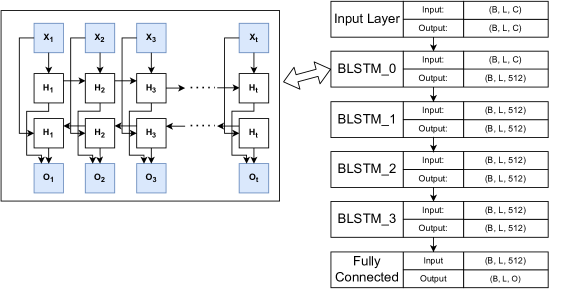
Figure 1: The architecture of bidirectional LSTM. The subfigure on the left represents a bidirectional LSTM cell. Here, B, L, C, O are batch size, the longest sequence length of a batch, feature size, and the number of output signal channels.

Figure 1 shows the deep learning model architecture stacked four bidirectional LSTMs. For any time step $t$, we define the mini-batch input as $\boldsymbol{X_{t}}\in\mathbb{R}^{n\times d}$ (number of examples: $n$ , number of input features in each example: $d$). In per layer bidirectional LSTM, the forward and backward hidden states for this time step are $\overrightarrow{\boldsymbol{H}}_{t}\in\mathbb{R}^{n\times h}$ and $\overleftarrow{\boldsymbol{H}}_{t}\in\mathbb{R}^{n\times h}$ , respectively, where $h$ is the hidden units number. $\overrightarrow{\boldsymbol{H}}_{t}\in\mathbb{R}^{n\times h}$ and $\overleftarrow{\boldsymbol{H}}_{t}\in\mathbb{R}^{n\times h}$ are updated with standard Bidirectional LSTM layer operations [43].

Next, the forward and backward hidden states $\overrightarrow{\boldsymbol{H}}_{t}$ and $\overleftarrow{\boldsymbol{H}}_{t}$ are concatenated to get the hidden state $\boldsymbol{H}_{t}\in\mathbb{R}^{n\times 2h}$ and fed it into the next layer. When we consider dropout, the hidden state $\boldsymbol{H}_{t}\in\mathbb{R}^{n\times 2h}$ will be randomly masked as zeros with a dropout rate $\delta$ of 0.1 at each step during the training phase. The dropout rate, as well as the other hyperparameters, have been optimized maxing the performance of the model on the validation set, according to the usual “hyperparameter tuning” procedure. The dropout can easily help prevent overfitting [47].

Last,output $\boldsymbol{O}_{t}\in\mathbb{R}^{n\times q}$(number of outputs: q) is computed as follows:

$$\boldsymbol{O}_{t}=activation(\boldsymbol{H}_{t}\boldsymbol{W}_{hq}+\boldsymbol{b}_{q}).$$ (1)

Here, the weight matrix $\boldsymbol{W}_{hq}\in\mathbb{R}^{2h\times q}$ and the bias $\boldsymbol{b}_{q}\in\mathbb{R}^{1\times q}$ are the model parameters of the output layer.

One of the key features of a bidirectional LSTM is that information from both directions of the sequence is used to estimate the current time step. The architecture uses future (forward) and past (backward) information to perform the inference. The final layer activation function is a linear function since we are dealing with a regression task and don’t want to constrain output parameters values.

3 Dataset

The whole EAST’s data system stores more than 3000 raw channel data and thousands of processed physical analysis data [48], which records the whole process of the EAST discharge. All the tokamak data was divided into three categories: configuration parameters, actuator signals, and diagnostic signals. The configuration parameters describe constants related to the tokamak such as magnetic probe positions. The actuator signals such as the power of ECRH, etc., are actively controlled quantities. The diagnostic signals are observable parameters passively measured from internal plasma such as loop voltage $V_{loop}$ etc. The configuration parameters are fixed during the tokamak experiments. The discharge prediction task can be essentially reduced to mapping actuator (input) signals to diagnostic (output) signals.

In the present work, the output signals include all important 0-D EAST diagnostic signals routinely available after a discharge. The input signals include all the quantities that may affect the output. Table 1 contains detailed information about input and output signals. The input signal “Ref. Shape”, in a particular, requires a more in depth discussion. According to the tokamak magnetic control system workflow [49], the shape references affect the in-vessel Rogowski coil current (IC1). So when estimating IC1, such shape references data is required. On EAST, shape feedback control is realized using the isoflux control scheme [50]. As the key concept of isoflux control, the plasma target shape (Ref. Shape) is interpreted as a set of control points defining the desired plasma boundary, and the flux at each control point is regulated to be equal. Usually, one of the control points is chosen as a reference point, which is typically a point on the limiter in a limited plasma configuration or the X point in a diverted configuration. Thus the plasma boundary is controlled by adjusting the PF coil currents to eliminate the flux error between the reference point and other boundary control points. Some of the selected signals are processed signals with clear physical meaning, and others are unprocessed raw electrical signals. Since some signals of the actual EAST experimental diagnostic system are not processed, we directly selected some unprocessed raw electrical signals. As long as the input signals include information to determine the output, the unprocessed signals will not affect the modeling result.

Table 1: The list of signals. The “raw signal” means the original electrical signal, and these could be converted to signals with physical meaning. The IC1 was estimated using a machine learning model and then fed to the diagnostic signals (output) reconstruction model as input.

Signals	Physics meanings	Unit	Number of Channels	Sampling rate	Meaning of Channels
Output Signals			12
$\text{Act.}I_{p}$	Actual plasma current	$A$	1	$1kHz$	Actual plasma current
$n_{e}$	Electron density	$10^{19}m^{-3}$	1	$1kHz$	Electron density
$W_{mhd}$	Plasma stored energy	$J$	1	$20Hz$	Plasma stored energy
$V_{loop}$	Loop voltage	$V$	1	$1kHz$	Loop voltage
$\beta_{n}$	Normalized beta	dimensionless	1	$15Hz$	Normalized beta
$\beta_{t}$	Toroidal beta	dimensionless	1	$15Hz$	Toroidal beta
$\beta_{p}$	Beta poloidal	dimensionless	1	$15Hz$	Beta poloidal
$\kappa$	Elongation at plasma boundary	dimensionless	1	$15Hz$	Elongation at plasma boundary
$l_{i}$	Internal inductance	dimensionless	1	$15Hz$	Internal inductance
$q_{0}$	q at magnetic axis	dimensionless	1	$15Hz$	q at magnetic axis
$q_{95}$	q at 95% flux surface	dimensionless	1	$15Hz$	q at 95% flux surface
Feedback Signal			1
IC1	In-vessel coil no.1 current	$A$	1	$1kHz$	In-vessel Rogowski coil no.1 current
Input Signals			95
Ref.$I_{p}$	Reference plasma current	$A$	1	$1kHz$	Reference plasma current
PF	Current of Poloidal field (PF) coils	$A$	14	$1kHz$	PF 0-14 current
$B_{t0}$	Toroidal magnetic field	$T$	1	$1kHz$	Toroidal field at magnetic axis
LHW	Power of Lower Hybrid Wave Current Drive and Heating System	$kW$	4	$20kHz$	2.45 GHz LHW, and 4.6 GHz LHW
NBI	Neutral Beam Injection System	Raw signal	8	$5kHz$	Acceleration voltage and beam current, of No. 1-2 left/right ion source.
ICRH	Ion Cyclotron Resonance Heating System	Raw signal	16	$5kHz$	Output of detector for rejected power of No. 1-16 transmitter
ECRH/ ECCD	Electron Cyclotron Resonance Heating/Current Drive System	Raw signal	4	$50kHz$	Output of detector for injected power measurement No. 1-4 gyrotron
GPS	Gas Puffing System	Raw signal	12	$10kHz$	Horizontal ports J, K, D, B; Upper port O; Lower ports O, C, H
SMBI	Supersonic Molecular Beam Injection	Raw signal	3	$10kHz$	3 ports of SMBI
PIS	Pellet Injection System	Raw signal	1	$10kHz$	1 injection line for Pellet Injection
Ref. Shape	Shape reference	Raw signal	31	$1kHz$	20 groups of control points

Tokamak discharge evolution is a multi-spatial-temporal scales, non-linear, multi-physics quantities coupling process. There is no simple function to determine the relationship between the actuator signals and the diagnostic signals. Different diagnostic parameters are determined by different inputs. In the present work, the input signals can not simply and directly determine all the output signals. In our model training experiments, $l_{i}$, $\beta_{p}$ can not be accurately estimated by the input signals that do not include IC1. When the input signals include the actual IC1, all output signals of the present work can be estimated. Since IC1 values cannot be obtained through direct measurement, they have been indirectly estimated through a machine learning model.

4 Training

This section shows details of model training and data processing. The training model is divided into four steps as follows:

1. Obtaining and resampling the data of the 108 data channels (including input, feedback, and output signals as shown in table 1) from the EAST source database, then storing it in HDF5 file with each HDF5 file data properties (standard deviation $\delta$, mean $\mu$, etc.) stored in MongoDB [51].

2. Standardizing the data with z-scores (also known as standard scores).

3. Using bucketing (explained further in section 4.3) batch training for the deep learning model to be reconstructed IC1.

4. Integrating the estimated IC1 as input for the eleven key diagnostic signals (table 1 output signals) reconstruction model training.

4.1 Obtaining and resampling

The dataset is selected from EAST tokamak during the 2010-2020 campaigns, and the discharge shot number is in the range #14866-88283 [39, 40, 41]. A total of 26230 normal shots were selected. “Normal shot” means that the plasma current is safely landed without disrupting and the flat-top duration is of at least two seconds. Moreover all the key quantities (i.e., magnetic field $B_{t}$, PF) describing the magnetic configuration as well as the actual plasma current are available for the entire duration of the shots. If there is not a certain magnetic field configuration, it is impossible to constrain (or control) the plasma. Furthermore, during a tokamak experiment, the actual $I_{p}$ is a key physical quantity, the experiment is generally considered a failure if there is no actual $I_{p}$. In model usage, actual $I_{p}$ is a output signal. Additionally, from a pure technical point of view, the training as well as the testing of the deep learning model cannot be performed if unless at least one output signal is available. Three different data sets are needed while developing the bidirectional LSTM model for discharge modeling. A training set is required for training the model. A validation set is needed for hyper-parameters tuning, whereas a test set is used to measure the final accuracy of the deep learning model, as well as its generalization capability. The training set should use the earliest data of the selected EAST campaign to simulate the new data faced in practice, as it always happens in practice. It is worth mentioning that, despite of the chronologically order, validation and test sets do not contain more recent pulse scheduling/piloting techniques with respect to what is not included in the training set. The capability of more advanced operations and control schemes as well as the target plasma evolve over the years according to the experimental program. For the sake of consistency, completely new control techniques and piloting schemes have not been considered for the evaluation of the current models. The test set and validation set are assumed to be statistically similar, so we can expect the best performance on the test set by optimizing the accuracy of the validation set. For each epoch, the model must input every shot in the validation set to get the performance metric, and the validation set is not used to update the model parameters. So relatively small validation set can accelerate the model training. The shot range of the validation set and the test set should not have any intersection to ensure the objectivity of the test set. The test set should only be used once, that is for assessing the real accuracy of the model. In other words, the test set should be used only for model testing and should not be present during the model training or tuning phase. These three data sets have been carefully selected to meet these strict requirements. Shot #14866-74999 in the EAST database is selected as the training set. 21192 normal shots are reserved at last. The validation set has shot numbers in the range #75000-77000. Shots #77000-88283 are in the test set.

All data are resampled with the same sample rate $1kHz$. Although we used a relatively low sampling rate, the original resampled data set still contains 55GB of data. Therefore for each shot, the data is saved to an HDF5 file, not in the database server for quick and robust training. The metadata is stored in MongoDB for double-checking the data validity and availability by the human and program.

We align our data with the same time axis by linearly interpolating to up-sample and a simple moving average (SMA) to down-sample. The simple moving average (SMA) is the unweighted mean of the $k$ data-points and works like a low-pass filter. Our SMA used the information from the later time. Since we use a bidirectional LSTM as architecture for the model and we aim to offline discharge modeling, we can remove the causality constraint for the sequences fed to the model for training. From another perspective, since high-frequency fluctuations are not a relevant outcome of the experimental proposal stage, we process the data by filtering out high-frequency fluctuations.

4.2 Data standardization

Firstly, all source data was saved in the HDF5 file. Then, discharge duration time and every signal mean, variance, and existence flag will be saved to the MongoDB database shot-by-shot. Saving the mean and variance of each signal of each shot data is necessary not only to double-check the presence of outliers in the signals but also for calculating the global means and standard deviations for the huge dataset by MapReduce [52]. If a signal in a shot has outliers, then the signal values in this shot will not be used to calculate the signal’s global mean and standard deviation. MapReduce is a programming model and an associated implementation for processing and generating big data sets with a parallel, distributed algorithm on a cluster. The reasons for using MapReduce are that if the global mean and standard deviation were calculated directly, the calculation would be overflowed. When the source data means and standard deviations have been calculated, the z-scores will be applied for standardization. In this step, if the input data have NaN (invalid value) or Inf (infinite value) will be replaced by a linear interpolation value and $3.2\text{$\times 10^{32}$}$(it is not the maximum value of the float 32 type, but it is large enough. And it can still be calculated without overflowing), respectively.

4.3 Bucketing batchwise training.

Mini-batching gradient descent [53, 54] is a valuable technique for enhancing GPU performance [55] and accelerating the training convergence of deep-learning models. The parameter loss gradients are computed for several examples in parallel and then averaged. However, this operation requires all examples have the same length. Therefore, training RNN or its variants on a large amount of data with different lengths is a quite challenging problem. Bucketing [56] was used to solve this problem in the present work.

The bucketing method can be reduced to a partition problem. Let $S=\left\{s_{1},s_{2},\ldots,s_{n}\right\}$ be sequences set and the length of sequence $s_{i}$ is $l_{i}=\left|s_{i}\right|$. Each GPU processes sequences in a mini-batch in a synchronized parallel manner, so processing time of a mini-batch $I_{\text{batch}}=\left\{s_{1},s_{2},\ldots,s_{k}\right\}$ is proportional to $O\left(\text{max}_{i\in 1,\ldots,k}l_{i}\right)$ and processing time of the whole set is expressed as:

$$T(S)=O\left(n/k*\text{max}_{i\in 1,\ldots,k}l_{i}\right).$$ (2)

If the dataset sequences were shuffled randomly before splitting, the minimum and maximum sequence lengths in the mini-batch would be very different. As a result, the GPU would do additional work for processing the meaningless tails of shorter sequences. Additionally, the too-long sequence with a non-suitable batch size will be overflowed due to the GPU memory capacity limit. Specifically, if we use the same batch size for long sequences input as for short sequences input, it will take up more GPU memory which will easily cause overflows. We used customized bucketing to optimize the batch training to overcome this flaw and reduce training time. As shown in figure 2, according to length, all sequences are partitioned to $B$ buckets. Let $S_{i}=\left\{s_{j_{1}},s_{j_{2}},\ldots s_{j_{k_{i}}}\right\}$. For each bucket, we execute the mini-batch training with different batch sizes. The processing time of the whole set is expressed as:

$$T(S)=\sum_{i=1}^{B}O(T(S_{i})).$$ (3)

We manually partitioned the sequence length set in the present work because the different sequence length sets will use different batch sizes. The result of the partition is shown in figure 2. Bucket 1,2,3 are in intervals $\left[2,12.3\right]$, $\left(12.3,50\right]$, and $\left(50,412\right]$ respectively. Because of the GPU memory capacity limit, the batch size of the three buckets is set at 8,4,1, respectively. These batch sizes can control GPU memory overflow and easily allocate the input tensor for each GPU.

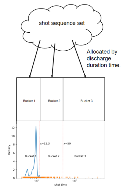
Figure 2: The shots during time distribution of the input discharge sequences. The number of buckets $B=3$. The y-axis represents distribution density, normalized as a probability density function.

The sequences within every bucket were shuffled randomly. And then, the sequences were generated batch-by-batch. To train batchwise with a batch size $M$, we need M independent shot discharge sequences of the same bucket to feed to the GPU. The different length discharge sequences were padded by zeros to the same length. We did this by using M processes to read sequence data in parallel. The M sequences were fed to a buffer first to solve the problem of GPU and CPU speed mismatch since data from HDF5 files are read through a CPU.

4.4 Model training

IC1 is an in-vessel Rogowski coil current [57, 49], and this current does not have a direct reference signal. In-vessel current distribution play a key role in the accuracy of reconstruction through a free boundary plasma equilibrium solver. The estimation of such in-vessel current distribution through simulation codes is very expensive and given the large number of discharges used to train and assess the performance of the model described in this paper, we decided to rely on the IC1 measured current, which acts basically as a proxy for the in-vessel current distribution. Although this might potentially introduce errors in the reconstruction of equilibrium quantities, it was found that not including IC1 in the set of input parameters heavily affected the accuracy of the reconstruction of quantities such as $\beta_{n}$, $\beta_{p}$ and $l_{i}.$ The IC1 signal can not be programmed or manually set in the experiment proposal stage. Therefore, first, we train a machine learning model (same model architect as depicted in figure 1) to reconstruct IC1. Secondly, we connected the trained IC1 reconstruction model and the diagnostic parameters reconstruction model for training, where the IC1 reconstruction part was fine-tuned using a minimal learning rate. For this reason, the output of the IC1 reconstruction model and the input IC1 to the deep learning model are different.

To facilitate fine-tuning the IC1 part, the model for reconstructing IC1 and the diagnostic parameters has the same architecture, initializer, optimizer, training set, validation set, test set, etc, in which only the input and output are different. The input of the IC1 reconstruction includes all input signals in table 1. The input of the diagnostic parameters reconstruction includes the output of the IC1 reconstruction model and does not use the shape reference signals. The training process is similar to using the trained model, as shown in figure 3.

The deep learning model uses end-to-end training executed on 8x Nvidia P100 GPUs with PyTorch [58] on the Centos7 operating system. The weight initialization scheme for the deep learning model is Xavier initialization [59], bias initializer is zeros, and optimizer is RMSprop [60]. The loss function of this training should be noted. The function is Masked MSELoss, which has some improvements for mean squared error (MSE) loss function. The MaskedMSEloss can be described as:

$$l\left(\boldsymbol{x},\boldsymbol{y}\right)=L=\frac{\sum_{i=0}^{i=N}\{l_{1},l_{2},\ldots,l_{N}\}}{N},$$ (4)

$$l_{i}=\sum_{j=0}^{j=\text{len}}\left(\boldsymbol{x}_{j}^{i}-\boldsymbol{y}_{j}^{i}\right)^{2},$$ (5)

where N is the batch size, $\boldsymbol{x}$ and $\boldsymbol{y}$ are the batch experimental sequence and batch predicted sequence, $\boldsymbol{x}_{j}^{i}$, $\boldsymbol{y}_{j}^{i}$ are the $j$th point values of the $i$th experimental sequence and predicted sequence. The subtlety of this work is “$j=\text{len}$”, where “len” is the length of the $i$th sequence. So the masked MSE function can prevent useless training of the zeros padding section of the sequence. In training our model, multiple sets of hyperparameters were tried. It was a trial-and-error approach on different sets of hyperparameters. The best hyperparameter set was selected based on the best performances of the validation set. Table 2 shows the best hyperparameter set.

Table 2: Our model Hyperparameters

Hyperparameter	Explanation	Best value
$\eta$	Normal learning rate	$3\times 10^{-3}$ or $5\times 10^{-3}$
$\eta_{f}$	Fine-tuning learning rate	$1\times 10^{-4}$
$\gamma$	Momentum factor	0.5
L2	L2 regularization rate	0.01
Loss function	Loss function type	Masked MSE
Optimizer	Optimization scheme	RMSprop
Dropout	Dropout probability	0.1
dt	Time step	1ms
Batch_size	Batch size	8,4,1
RNN_type	Type of RNN	Bidirectional LSTM
$n_{rnn}$	Number of RNN stacked	4
$H_{rnn}$	Hidden size of RNN	512
$n_{encoder}$	Number of BiLSTMs stacked in encoder	2
$n_{decoder}$	Number of BiLSTMs stacked in decoder	2

5 Results

The model was tested on unseen data (test set), as shown in figure 3. In the present work, models are used in sequence. The #1 deep learning model is used first to get the IC1 estimated values and then the #2 deep learning model to estimate the tokamak’s main diagnostic signals. The preprocessing steps on new data are the same as before, keeping the training set parameters (the mean $\mu$ and the standard deviation $\sigma$) for standardization.

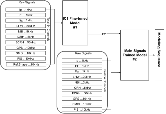
Figure 3: Using the trained model.

This section details the results and analyzes. The results include representative modeling results and eleven diagnostic signal similarity distributions of the test set. Additionally, the present work uses similarity and means square error (MSE) as quantitative measurements of the accuracy of the modeling results.

$$S\left(\boldsymbol{x},\boldsymbol{y}\right)=\max\left(\frac{\Sigma(\boldsymbol{x}-\bar{\boldsymbol{x}})(\boldsymbol{y}-\bar{\boldsymbol{y}})}{\sqrt{\Sigma(\boldsymbol{x}-\bar{\boldsymbol{x}})^{2}\Sigma(\boldsymbol{y}-\bar{\boldsymbol{y}})^{2}}},0\right),$$ (6)

$$MSE\left(\boldsymbol{x},\boldsymbol{y}\right)=\frac{1}{n}\sum_{i=1}^{n}(\boldsymbol{x}_{i}-\boldsymbol{y}_{i})^{2},$$ (7)

where $\boldsymbol{x}$ is experimental data, $\boldsymbol{y}$ is modeling result, $\bar{\boldsymbol{x}}$, $\bar{\boldsymbol{y}}$ are the means of the vector $\boldsymbol{x}$ and vector $\boldsymbol{y}$, $\boldsymbol{x}_{i}$, $\boldsymbol{y}_{i}$ are the point values of the vector $\boldsymbol{x}$, $\boldsymbol{y}$. The MSE is the mean ($\frac{1}{n}\sum_{i=1}^{n}$) of the squares of the errors $(\boldsymbol{x}_{i}-\boldsymbol{y}_{i})^{2}$. MSE will be affected by the outlier but it can more accurately measure the difference of values. Similarity can only measure whether the trend is consistent, but it cannot measure the difference in value.

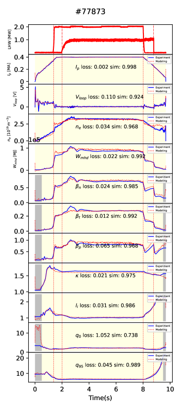
Figure 4: Comparison of the modeling result and EAST experiment data. “sim” is similarity (equation 6) and “loss” is MSE (equation 7). Shot #77873 have two LHW injections during discharge. No experimental data are available for the gray area, so the modeling results for this area are unreliable. During model training, we used the start value and end value to fill these areas for time axis alignment.

A typical entire process discharge prediction of our model is shown in figure 4. In the present work, the trained model can reproduce the eleven diagnostic signals during experimental proposal stage, from ramp-up to ramp-down, without relying on any physical codes.

Figure 4 shows our model can accurately reproduces the slopes of the ramp-up and ramp-down and the amplitude of the flat-top. The model can also reflect the external auxiliary system signal impact on the diagnostic signal. The vertical dash-dot lines of figure 4 indicate the rising and falling edges of the external auxiliary system signals and the plasma response.

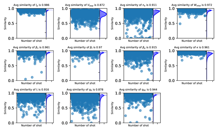
Figure 5: The similarity distribution and average similarity in the whole test set. The figure shows the similarity distributions of the output signals (see table 1)

Table 3: The average similarity and MSE of the eleven diagnostic signals.

Output signals	Average similarity	Average MSE
$\text{Act.}I_{p}$	0.986	0.0015
$n_{e}$	0.911	0.341
$W_{mhd}$	0.972	0.077
$V_{loop}$	0.872	0.354
$\beta_{n}$	0.961	0.062
$\beta_{t}$	0.970	0.130
$\beta_{p}$	0.915	0.179
$\kappa$	0.961	0.0019
$l_{i}$	0.916	0.127
$q_{0}$	0.878	0.129
$q_{95}$	0.944	0.093

The whole test data set of shot range 77000-88283 is used to quantitatively evaluate the reliability of the modeling results of the eleven signals. The statistical results of the similarity and MSE between modeling results and experimental data are shown in figure 5 and table 3. Except for $q_{0}$ and $V_{loop}$, the average similarity of other key signals is greater than 90%. And the similarity distribution is concentrated above 90%. The average similarity of $q_{0}$ is greater than 85%. This quantity has a poor similarity, because if the equilibrium reconstruction is not properly constrained with pressure profiles and kinetic measurements, $q_{0}$ might be unreliable. Since it might suffer from large variance, as the model is struggling mostly for the reconstruction of that parameter. Most of the errors in the reconstruction of $V_{loop}$ are related to the plasma start-up and shut-down phases. To sum up, all selected key diagnostic signals, excluding $V_{loop}$ are regarded as almost wholly predicted.

6 Conclusion and discussion

In the present work, we propose a tokamak discharge prediction method based on bidirectional LSTM. The bidirectional LSTM was developed to introduce the wider contextual information of discharge sequence to achieve a more efficient model. The model was trained on the EAST experimental dataset in shot range #14866-88283. This model can use the actuator signals to reproduce the normal discharge evolution process of the eleven key signals (i.e., actual plasma current $I_{p}$, normalized beta $\beta_{n}$, toroidal beta $\beta_{t}$, beta poloidal $\beta_{p}$, electron density $n_{e}$, store energy $W_{mhd}$, loop voltage $V_{loop}$, elongation at plasma boundary $\kappa$, internal inductance $l_{i}$, q at magnetic axis $q_{0}$, and q at 95% flux surface $q_{95}$.) without having as input any quantity derived by physical models. Bidirectional LSTM architecture is robust to outliers. The average similarities of all the selected key diagnostic signals between modeling results and the experimental data are greater than 90%, except for the $V_{loop}$ and $q_{0}$. The results presented in this paper demonstrate the effectiveness of using a purely data-driven model to assist the validation of the experimental proposal for a tokamak discharge.

The present work demonstrates that the model can easily be extended to more diagnostic signals. Compared with physical models, experimental data-driven models have proven to be very efficient computationally. Once the machine learning model has been trained, a run of the trained machine learning model is faster by orders of magnitude with respect to the whole process of tokamak discharge modeling. The total inference time of our model for an entire discharge prediction is about 1s. The present work shows very promising results exploiting experimental data-driven modeling as a supplement to physical-driven modeling tokamak. Another important point which is worth mentioning is that our model currently uses a smoothed version of the measured actuator signals as input. and not directly the corresponding programmed PCS trajectories. A complete understanding of the actuator trajectories prior to a shot is challenging. The feasibility of using programmed PCS trajectories as model input to predict the evolution of a tokamak discharge will be the object of future work. Besides, we want to integrate the model into the plasma control system (PCS) to automatically check the control strategy. 1D and 2D plasma profiles (kinetic quantities, radiation distribution) are also particularly important for tokamak discharge modeling, since they can support scenario development with particular reference to operational limits in high-performance scenarios [61].

References

- [1] G.L. Falchetto, David Coster, Rui Coelho, B.D. Scott, Lorenzo Figini, Denis Kalupin, Eric Nardon, Silvana Nowak, L.L. Alves, J.F. Artaud, V. Basiuk, João P.S. Bizarro, C. Boulbe, A. Dinklage, D. Farina, B. Faugeras, J. Ferreira, A. Figueiredo, Ph Huynh, F. Imbeaux, I. Ivanova-Stanik, T. Jonsson, H.-J. Klingshirn, C. Konz, A. Kus, N.B. Marushchenko, G. Pereverzev, M. Owsiak, E. Poli, Y. Peysson, R. Reimer, J. Signoret, O. Sauter, R. Stankiewicz, P. Strand, I. Voitsekhovitch, E. Westerhof, T. Zok, and W. Zwingmann. The European Integrated Tokamak Modelling (ITM) effort: achievements and first physics results. Nuclear Fusion, 54(4):043018, apr 2014.
- [2] Paul Bonoli, Lois Curfman McInnes, C Sovinec, D Brennan, T Rognlien, P Snyder, J Candy, C Kessel, J Hittinger, and L Chacon. Report of the Workshop on Integrated Simulations for Magnetic Fusion Energy Sciences. Technical report, Massachusetts Institute of Technology, 2015.
- [3] Julian Kates-Harbeck, Alexey Svyatkovskiy, and William Tang. Predicting disruptive instabilities in controlled fusion plasmas through deep learning. Nature, 568(7753):526–531, apr 2019.
- [4] W.H. H. Hu, Cristina Rea, Q.P. P. Yuan, K.G. G. Erickson, D.L. L. Chen, Biao Shen, Yao Huang, J.Y. Y. Xiao, J.J. J. Chen, Y.M. M. Duan, Yang Zhang, H.D. D. Zhuang, J.C. C. Xu, K.J. J. Montes, R.S. S. Granetz, Long Zeng, J.P. P. Qian, B.J. J. Xiao, and J.G. G. Li. Real-time prediction of high-density EAST disruptions using random forest. Nuclear Fusion, 61(6):066034, jun 2021.
- [5] Bihao H Guo, Dalong L Chen, Biao Shen, Cristina Rea, Robert S Granetz, Long Zeng, Wenhui H Hu, Jinping P Qian, Youwen W Sun, and Bingjia J Xiao. Disruption prediction on EAST tokamak using a deep learning algorithm. Plasma Physics and Controlled Fusion, 63(11):115007, nov 2021.
- [6] B. Cannas, A. Fanni, P. Sonato, and M.K. Zedda. A prediction tool for real-time application in the disruption protection system at JET. Nuclear Fusion, 47(11):1559–1569, nov 2007.
- [7] Barbara Cannas, R.S. Delogu, ALESSANDRA Fanni, P Sonato, and M.K. Zedda. Support vector machines for disruption prediction and novelty detection at JET. Fusion Engineering and Design, 82(5-14):1124–1130, oct 2007.
- [8] Barbara Cannas, Alessandra Fanni, G Pautasso, G Sias, and P Sonato. An adaptive real-time disruption predictor for ASDEX Upgrade. Nuclear Fusion, 50(7):075004, jul 2010.
- [9] R Yoshino. Neural-net disruption predictor in JT-60U. Nuclear Fusion, 43(12):1771–1786, dec 2003.
- [10] D. J. Clayton, K. Tritz, D. Stutman, R. E. Bell, A. Diallo, B P LeBlanc, and M. Podestà. Electron temperature profile reconstructions from multi-energy SXR measurements using neural networks. Plasma Physics and Controlled Fusion, 55(9):095015, sep 2013.
- [11] O Barana, A Murari, P Franz, L C Ingesson, and G Manduchi. Neural networks for real time determination of radiated power in JET. Review of Scientific Instruments, 73(5):2038–2043, may 2002.
- [12] B Cannas, S Carcangiu, A Fanni, T Farley, F Militello, A Montisci, F Pisano, G Sias, and N Walkden. Towards an automatic filament detector with a Faster R-CNN on MAST-U. Fusion Engineering and Design, 146:374–377, sep 2019.
- [13] M. Honda and E. Narita. Machine-learning assisted steady-state profile predictions using global optimization techniques. Physics of Plasmas, 26(10):102307, oct 2019.
- [14] O Meneghini, S P Smith, P B Snyder, G M Staebler, J Candy, E Belli, L Lao, M Kostuk, T Luce, T Luda, J M Park, and F Poli. Self-consistent core-pedestal transport simulations with neural network accelerated models. Nuclear Fusion, 57(8):86034, jul 2017.
- [15] O. Meneghini, G. Snoep, B.C. Lyons, J. McClenaghan, C.S. Imai, B. Grierson, S.P. Smith, G.M. Staebler, P.B. Snyder, J. Candy, E. Belli, L. Lao, J.M. Park, J. Citrin, T.L. Cordemiglia, A. Tema, and S. Mordijck. Neural-network accelerated coupled core-pedestal simulations with self-consistent transport of impurities and compatible with ITER IMAS. Nuclear Fusion, 61(2):026006, feb 2021.
- [16] A Murari, D Mazon, N Martin, G Vagliasindi, and M Gelfusa. Exploratory Data Analysis Techniques to Determine the Dimensionality of Complex Nonlinear Phenomena: The L-to-H Transition at JET as a Case Study. IEEE Transactions on Plasma Science, 40(5):1386–1394, may 2012.
- [17] Diogo R Ferreira and Pedro J Carvalho. Deep Learning for Plasma Tomography in Nuclear Fusion. pages 1–5, 2020.
- [18] A Murari, P Arena, A Buscarino, L Fortuna, and M Iachello. On the identification of instabilities with neural networks on JET. Nuclear Instruments and Methods in Physics Research Section A: Accelerators, Spectrometers, Detectors and Associated Equipment, 720:2–6, aug 2013.
- [19] M.D. Boyer, S. Kaye, and K. Erickson. Real-time capable modeling of neutral beam injection on NSTX-U using neural networks. Nuclear Fusion, 59(5):056008, may 2019.
- [20] A Murari, J Vega, D Mazon, D Patané, G Vagliasindi, P Arena, N Martin, N F Martin, G Rattá, and V Caloone. Machine learning for the identification of scaling laws and dynamical systems directly from data in fusion. Nuclear Instruments and Methods in Physics Research Section A: Accelerators, Spectrometers, Detectors and Associated Equipment, 623(2):850–854, 2010.
- [21] P Gaudio, A Murari, M Gelfusa, I Lupelli, and J Vega. An alternative approach to the determination of scaling law expressions for the L{textendash}H transition in Tokamaks utilizing classification tools instead of regression. Plasma Physics and Controlled Fusion, 56(11):114002, oct 2014.
- [22] Daniel Böckenhoff, Marko Blatzheim, Hauke Hölbe, Holger Niemann, Fabio Pisano, Roger Labahn, and Thomas Sunn Pedersen. Reconstruction of magnetic configurations in W7-X using artificial neural networks. Nuclear Fusion, 58(5):56009, mar 2018.
- [23] E Coccorese, C Morabito, and Raffaele Martone. Identification of noncircular plasma equilibria using a neural network approach. Nuclear Fusion, 34(10):1349–1363, oct 1994.
- [24] Chris M Bishop, Paul S Haynes, Mike E U Smith, Tom N Todd, and David L Trotman. Fast feedback control of a high temperature fusion plasma. Neural Computing & Applications, 2(3):148–159, sep 1994.
- [25] Young-Mu Jeon, Yong-Su Na, Myung-Rak Kim, and Y S Hwang. Newly developed double neural network concept for reliable fast plasma position control. Review of Scientific Instruments, 72(1):513–516, jan 2001.
- [26] S Y Wang, Z Y Chen, D W Huang, R H Tong, W Yan, Y N Wei, T K Ma, M Zhang, and G Zhuang. Prediction of density limit disruptions on the J-TEXT tokamak. Plasma Physics and Controlled Fusion, 58(5):055014, may 2016.
- [27] Semin Joung, Jaewook Kim, Sehyun Kwak, J. G. Bak, S. G. Lee, H. S. Han, H. S. Kim, Geunho Lee, Daeho Kwon, and Y.-C. C. Ghim. Deep neural network Grad-Shafranov solver constrained with measured magnetic signals. Nuclear Fusion, 60(1):16034, dec 2020.
- [28] B Ph. van Milligen, V Tribaldos, and J A Jiménez. Neural Network Differential Equation and Plasma Equilibrium Solver. Phys. Rev. Lett., 75(20):3594–3597, nov 1995.
- [29] Chris M Bishop, Paul S Haynes, Mike E U Smith, Tom N Todd, and David L Trotman. Real-time control of a tokamak plasma using neural networks. Neural Computation, 7(1):206–217, 1995.
- [30] Bin Yang, Zhenxing Liu, Xianmin Song, and Xiangwen Li. Design of {HL}-2A plasma position predictive model based on deep learning. Plasma Physics and Controlled Fusion, 62(12):125022, nov 2020.
- [31] T. Wakatsuki, T. Suzuki, N. Hayashi, N. Oyama, and S. Ide. Safety factor profile control with reduced central solenoid flux consumption during plasma current ramp-up phase using a reinforcement learning technique. Nuclear Fusion, 59(6):066022, jun 2019.
- [32] H. Rasouli, C. Rasouli, and A. Koohi. Identification and control of plasma vertical position using neural network in Damavand tokamak. Review of Scientific Instruments, 84(2):023504, feb 2013.
- [33] Bin Yang, Zhenxing Liu, Xianmin Song, Xiangwen Li, and Yan Li. Modeling of the HL-2A plasma vertical displacement control system based on deep learning and its controller design. Plasma Physics and Controlled Fusion, 62(7):75004, jul 2020.
- [34] Jaemin Seo, Y.-S. Na, B. Kim, C.Y. Lee, M.S. Park, S.J. Park, and Y.H. Lee. Feedforward beta control in the KSTAR tokamak by deep reinforcement learning. Nuclear Fusion, 61(10):106010, oct 2021.
- [35] A. Mathews, M. Francisquez, J. W. Hughes, D. R. Hatch, B. Zhu, and B. N. Rogers. Uncovering turbulent plasma dynamics via deep learning from partial observations. Physical Review E, 104(2):025205, aug 2021.
- [36] Chenguang Wan, Zhi Yu, Feng Wang, Xiaojuan Liu, and Jiangang Li. Experiment data-driven modeling of tokamak discharge in EAST. Nuclear Fusion, 61(6):066015, jun 2021.
- [37] S C Jardin, M G Bell, N Pomphrey, Home Search, Collections Journals, About Contact, My Iopscience, I P Address, S C Jardin, M G Bell, and N Pomphrey. TSC simulation of Ohmic discharges in TFTR. Nuclear Fusion, 33(3):371–382, mar 1993.
- [38] S.C Jardin, N Pomphrey, and J Delucia. Dynamic modeling of transport and positional control of tokamaks. Journal of Computational Physics, 66(2):481–507, oct 1986.
- [39] Baonian Wan, Jiangang Li, Houyang Guo, Yunfeng Liang, Guosheng Xu, Liang Wang, and Xianzu Gong. Advances in H-mode physics for long-pulse operation on {EAST}. Nuclear Fusion, 55(10):104015, jul 2015.
- [40] Baonian Wan, Jiangang Li, Houyang Guo, Yunfeng Liang, and Guosheng Xu. Progress of long pulse and H-mode experiments in EAST. Nuclear Fusion, 53(10):104006, oct 2013.
- [41] Jiangang Li and Baonian Wan. Recent progress in RF heating and long-pulse experiments on EAST. Nuclear Fusion, 51(9):094007, sep 2011.
- [42] Trias Thireou and Martin Reczko. Bidirectional Long Short-Term Memory Networks for Predicting the Subcellular Localization of Eukaryotic Proteins. IEEE/ACM Transactions on Computational Biology and Bioinformatics, 4(3):441–446, jul 2007.
- [43] Mike Schuster and K.K. Paliwal. Bidirectional recurrent neural networks. IEEE Transactions on Signal Processing, 45(11):2673–2681, 1997.
- [44] Alex Graves and Jürgen Schmidhuber. Framewise phoneme classification with bidirectional LSTM and other neural network architectures. Neural Networks, 18(5-6):602–610, jul 2005.
- [45] Rusul L. Abduljabbar, Hussein Dia, and Pei-Wei Tsai. Development and evaluation of bidirectional LSTM freeway traffic forecasting models using simulation data. Scientific Reports, 11(1):23899, dec 2021.
- [46] Sima Siami-Namini, Neda Tavakoli, and Akbar Siami Namin. The Performance of LSTM and BiLSTM in Forecasting Time Series. In 2019 IEEE International Conference on Big Data (Big Data), pages 3285–3292. IEEE, dec 2019.
- [47] Nitish Srivastava, Geoffrey Hinton, Alex Krizhevsky, Ilya Sutskever, and Ruslan Salakhutdinov. Dropout: A simple way to prevent neural networks from overfitting. Journal of Machine Learning Research, 15(1):1929–1958, 2014.
- [48] Feng Wang, Yueting Wang, Ying Chen, Shi Li, and Fei Yang. Study of web-based management for EAST MDSplus data system. Fusion Engineering and Design, 129(June 2017):88–93, apr 2018.
- [49] Gianmaria De Tommasi. Plasma Magnetic Control in Tokamak Devices. Journal of Fusion Energy, 38(3-4):406–436, aug 2019.
- [50] H Anand, D Humphreys, D Eldon, A Leonard, A Hyatt, B Sammuli, and A Welander. Plasma flux expansion control on the DIII-D tokamak. Plasma Physics and Controlled Fusion, 63(1):015006, jan 2021.
- [51] MongoDB main page.
- [52] Jeffrey Dean and Sanjay Ghemawat. MapReduce. Communications of the ACM, 51(1):107–113, jan 2008.
- [53] Jeffrey Dean, Greg S Corrado, Rajat Monga, Kai Chen, Matthieu Devin, Quoc V Le, Mark Z Mao, Marc’Aurelio Marc’aurelio Ranzato, Andrew Senior, Paul Tucker, Others, and Ke Yang. Large scale distributed deep networks. Advances in neural information processing systems, 25:1223–1231, 2012.
- [54] Zhiheng Huang, Geoffrey Zweig, Michael Levit, Benoit Dumoulin, Barlas Oguz, and Shawn Chang. Accelerating recurrent neural network training via two stage classes and parallelization. In 2013 IEEE Workshop on Automatic Speech Recognition and Understanding, pages 326–331. IEEE, dec 2013.
- [55] Sharan Chetlur, Cliff Woolley, Philippe Vandermersch, Jonathan Cohen, John Tran, Bryan Catanzaro, and Evan Shelhamer. cuDNN: Efficient Primitives for Deep Learning. oct 2014.
- [56] Viacheslav Khomenko, Oleg Shyshkov, Olga Radyvonenko, and Kostiantyn Bokhan. Accelerating recurrent neural network training using sequence bucketing and multi-GPU data parallelization. In 2016 IEEE First International Conference on Data Stream Mining & Processing (DSMP), pages 100–103. IEEE, aug 2016.
- [57] B.J. Xiao, D.A. Humphreys, M.L. Walker, A. Hyatt, J.A. Leuer, D. Mueller, B.G. Penaflor, D.A. Pigrowski, R.D. Johnson, A. Welander, Q.P. Yuan, H.Z. Wang, J.R. Luo, Z.P. Luo, C.Y. Liu, L.Z. Liu, and K. Zhang. EAST plasma control system. Fusion Engineering and Design, 83(2-3):181–187, apr 2008.
- [58] Adam Paszke, Sam Gross, Francisco Massa, Adam Lerer, James Bradbury, Gregory Chanan, Trevor Killeen, Zeming Lin, Natalia Gimelshein, Luca Antiga, Alban Desmaison, Andreas Kopf, Edward Yang, Zachary DeVito, Martin Raison, Alykhan Tejani, Sasank Chilamkurthy, Benoit Steiner, Lu Fang, Junjie Bai, and Soumith Chintala. PyTorch: An Imperative Style, High-Performance Deep Learning Library. In H Wallach, H Larochelle, A Beygelzimer, F dtextquotesingle Alché-Buc, E Fox, and R Garnett, editors, Advances in Neural Information Processing Systems 32, pages 8024–8035. Curran Associates, Inc., 2019.
- [59] Xavier Glorot and Yoshua Bengio. Understanding the difficulty of training deep feedforward neural networks. In Journal of Machine Learning Research, volume 9, pages 249–256, 2010.
- [60] Alex Graves. Generating Sequences With Recurrent Neural Networks. aug 2013.
- [61] A. Pau, A. Fanni, S. Carcangiu, B. Cannas, G. Sias, A. Murari, F. Rimini, Human Immunodeficiency Virus, Associated Neurocognitive Disorders, Consensus Report, Mind Corresponding Author, and Alternate Corresponding Author. A machine learning approach based on generative topographic mapping for disruption prevention and avoidance at JET. Nuclear Fusion, 59(10):106017, oct 2019.