Statistical tests of young radio pulsars with/without supernova remnants: implying two origins of neutron stars

Abstract

The properties of the young pulsars and their relations to the supernova remnants (SNRs) have been the interesting topics. At present, 383 SNRs in the Milky Way galaxy have been published, which are associated with 64 radio pulsars and 46 pulsars with high energy emissions. However, we noticed that 630 young radio pulsars with spin periods of less than half a second have been not yet observed the SNRs surrounding or nearby them, which arises a question of that could the two types of young radio pulsars with/without SNRs hold distinctive characteristics? Here, we employ the statistical tests on the two groups of young radio pulsars with (52) and without (630) SNRs to reveal if they share different origins. Kolmogorov-Smirnov (K-S) and Mann-Whitney-Wilcoxon (M-W-W) tests indicate that the two samples have the different distributions with parameters of spin period ($P$), derivative of spin period ($\dot{P}$), surface magnetic field strength ($B$), and energy loss rate ($\dot{E}$). Meanwhile, the cumulative number ratio between the pulsars with and without SNRs at the different spindown ages decreases significantly after $\rm 10-20\,Kyr$. So we propose that the existence of the two types of supernovae (SNe), corresponding to their SNR lifetimes, which can be roughly ascribed to the low-energy and high-energy SNe. Furthermore, the low-energy SNe may be formed from the $\rm 8-12\,M_{\odot}$ progenitor, e.g., possibly experiencing the electron capture, while the main sequence stars of $\rm 12-25\,M_{\odot}$ may produce the high-energy SNe probably by the iron core collapse.

1 Introduction

The associations between the pulsars and supernova remnants (SNRs) have been of considerable interest topics in neutron stars (NSs) astrophysics, since the radio pulses were firstly observed in the Crab Nebula in 1968 (Staelin & Reifenstein 1968), as well as the discovery of the Vela pulsar (Large, Vaughan, & Mills 1968). The story is continuing with identifying the potential NS in SN 1987A (Page et al. 2020; Greco et al. 2021; Soker 2021). Thanks the efforts and developments of astronomical facilities in recent years, the number of pulsars and SNRs has increased significantly. Up to now, there are more than 3000 pulsars (ATNF: 2781, GPPS: 201 (Han et al. 2021), CRAFT: 125) observed in the radio band and 383 SNRs (SNRcat) in the Milky Way galaxy had been published (Ferrand & Safi-Harb 2012). Among these, there are 110 pulsars that have been identified in SNRs, including 6 anomalous X-ray pulsars (AXPs), 5 soft gamma-ray repeaters (SGRs), a total of 13 magnetar candidates, and 15 central compact objects (CCOs) or CCO candidates. By comparing with ANTF Pulsar Catalogue, there are also 18 pulsars without radio emissions (NRAD) in SNRcat, only observed at the infrared or higher frequencies (Manchester et al. 2005). In short, 64 radio pulsars with SNRs have been published, as seen in Table 1. Interestingly, the number ratio between the radio pulsars (64) and SNRs (337) is about 1/5, which is consistent with the estimation by the beaming fraction of radio pulsars (Taylor & Manchester 1977; Lorimer et al. 1993; Lorimer & Kramer 2012).

Table 1: List of various types of pulsars with SNRs

Source	Number	Ref.
SNR	383	[1]
Pulsara	110	[1]
Radio pulsar	64b	[2]
Magnetar or candidate	13c	[1, 3, 4]
CCOd or candidate	15	[1]
NRADe	18	[2]

Note:
^a Various pulsars with SNRs.

^b The total number of radio pulsars with SNRs is 64, but only 52 of them are analyzed in this article (selection details in Section 2.1).

^c AXP (anomalous X-ray pulsar): 6, SGR (soft gamma-ray repeater): 5. http://www.physics.mcgill.ca/~pulsar/magnetar/main.html

^d CCO: central compact object.

^e Pulsars without radio emissions and do not contain the magnetars, CCOs, and their candidates.

Ref.: [1] Ferrand & Safi-Harb (2012); [2] Manchester et al. (2005); [3] Olausen & Kaspi (2014); [4] Esposito, Rea, & Israel (2021).

From Table 1, the question of why only a fraction of SNRs have been found with pulsars can be solved by their beaming cone angles across the earth. Meanwhile, some other explanations are worthy of mentioning as pointed out as below. First of all, not every SNe could generate a NS or some NSs might not be detectable as pulsars (Radhakrishnan & Srinivasan 1980; Srinivasan, Bhattacharya, & Dwarakanath 1984; Manchester 1987; Narayan & Schaudt 1988). Next, the flux density or luminosity of young radio pulsars may be overestimated, implying that some young radio pulsars are too faint to be observed in some SNRs (Stollman 1987; Lorimer et al. 1993). Finally, the kick velocity of pulsar may be quite high after birth, which could result in the pulsars to escape from their SNRs (Frail, Goss, & Whiteoak 1994).

Although some pulsars can be found in the pulsar wind nebulae (Gaensler & Slane 2006), it is still an open question that so many young radio pulsars have not seen their SNRs. Nowadays, there exist 630 young radio pulsars (spin period less than 0.5 s, and details as described in Section 2) without SNRs, which provides us a new aspect to further study the association between pulsars and SNRs, as well as the NS origins. In the former studies of X-ray pulsars (Knigge, Coe, & Podsiadlowski 2011) and double neutron star (DNS) (Yang et al. 2019) population, researchers suggested that the NSs may birth from the different origins, i.e., the existence of the electron capture and iron core collapse SNe (Janka 2012). In the recent work about pulsars and SNRs, Malov (2021) noticed that the mean values of radio luminosity of pulsars observed inside and outside SNRs are significantly different with one order of magnitude.

Inspired by these researches, we conjecture that there may exist two origins for radio pulsars. Therefore, we attempt to use the statistical methods to study the properties of radio pulsars and their relations with SNRs. We apply some physical criteria to select two samples of pulsars, that is, the radio pulsars with SNR (SNR-PSRs, 52) and without SNR (non SNR-PSRs, 630) (see Section 2.1 for details) By drawing the cumulative distribution function (CDF) and utilizing the Kolmogorov-Smirnov (K-S) and Mann-Whitney-Wilcoxon (M-W-W) tests for these two samples, we find that the obtained results support the different distributions for two samples. Based on spin period evolution model, we estimate the spindown age (not characteristic age) of radio pulsars in these two samples. After a further discussion, it is inferred that the two samples of pulsars may origin from two types of progenitors, such as the low-energy and high-energy SNe (e.g., electron capture and iron core collapse), respectively. However, the energy boundary is still unclear, or there may be an overlapping part between them, because some researches in SNRs indicated that SNRs may have a continuous energy distribution like lognormal (Leahy 2017; Leahy, Ranasinghe, & Gelowitz 2020). Meanwhile, we notice that the cumulative number ratios of SNR-PSRs to non SNR-PSRs are decreased quickly after $\rm 10-20\,Kyr$. Finally, according to the initial mass function (IMF) or Salpeter function (Salpeter 1955), it is possible to statistically distinguish the two types of their progenitor stars at the mass boundary of $\rm\sim 12\,M_{\odot}$.

The structure of our paper is presented as follows. In Section 2, we describe the data selection of pulsars and introduce the spin period evolution model. In Section 3, we apply the statistical tests on the two samples and analyze the results. Finally, in Section 4, we discuss a possible physical significance for the two distributions of the pulsars, and main conclusions are summarized also.

2 Data and Model

2.1 Data Selection

Our data are taken from ATNF Pulsar Catalogue (Manchester et al. 2005) and SNRcat (Ferrand & Safi-Harb 2012). Data selections are made to construct the two samples of the young radio pulsars with and without SNRs, and the selection criteria are described below.

1) We choose the pulsar samples in the two data bases with the spin periods ($P$) less than 0.5 s. Due to the short duration of SNRs, the pulsars with SNRs are taken as the young pulsars (Gaensler & Johnston 1995; Malov 2021). Considering that the characteristic age of pulsar usually has a significant error compared to the real age (Lai 1996; Kaspi et al. 2001; Tian & Leahy 2006; Lyne & Graham-Smith 2012), we apply the spin period to represent the age under the spin period evolution model (details in Section 2.2). Generally speaking, the lifetime of SNRs usually less than 300 Kyr, so the spin period of pulsars may be around 0.5 s based on the magnetic dipole model (see Section 2.2 and Appendix A for calculation details). Meanwhile, for all radio pulsars, the median of period is about 0.5 s, which can be known from ATNF database (Manchester et al. 2005). Additionally, because the periods for most rotating radio transients (RRATs) and intermittent pulsars are greater than 0.5 s (McLaughlin et al. 2006; Kramer et al. 2006), we eliminate these special radio pulsars from our samples. Therefore, we regard the radio pulsars with spin periods of less than 0.5 s to be the young pulsar, and they are roughly consistent with the arguments based on that their magnetic fields are comparable with those measured by cyclotron absorption lines of X-rays (Ye et al. 2019).

2) The data with the surface magnetic field strength ($B$) ranged from $\rm 10^{11}\,G$ to $\rm 10^{14}\,G$ are used. If the pulsar’s B-field is lower than $\rm 10^{11}\,G$, it may be a millisecond pulsar (MSP) (Bhattacharya & van den Heuvel 1991; Lorimer 2008) or a CCO (Halpern & Gotthelf 2010; Gotthelf, Halpern, & Alford 2013). If the pulsar’s B-field is higher than $\rm 10^{14}\,G$, it may be a magnetar (Duncan & Thompson 1992; Ferrario & Wickramasinghe 2008; Kaspi & Beloborodov 2017; Esposito, Rea, & Israel 2021).

3) We select the data to satisfy that their spin periods and magnetic fields are distributed above the spin-up line in B-P diagram (Bhattacharya & van den Heuvel 1991). While, the pulsars below the spin-up line may have a more complicated evolutionary tracks, such as experiencing the accretion spin-up in binary systems (Zhang & Kojima 2006).

4) Some types of the special pulsars are removed from our samples, including the MSPs, magnetars, recycled pulsars (Zhang & Kojima 2006), CCOs, RRATs, intermittent pulsars and NRADs. The physical characteristics between the young radio pulsars and these special pulsars are significantly different, so they may follow the different birth conditions and evolutionary paths.

After setting these selections ($P<0.5s$, $10^{11}G<B<10^{14}G$, above the spin-up line, and removing the special pulsars), we obtain the two groups of samples of 52 SNR-PSRs and 630 non SNR-PSRs, respectively, as illustrated in Figure 1.

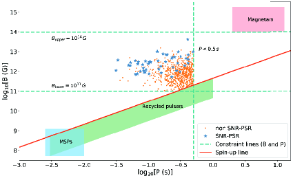
Figure 1: Data distribution graph in the magnetic field versus spin period (B-P) diagram after the selection criteria. The blue stars and orange dots stand for the SNR-PSRs and non SNR-PSRs, respectively. The green dashed lines represent the constraint lines of surface B-field strength (B) upper ($B_{upper}=\rm 10^{14}\,G$) and lower ($B_{lower}=\rm 10^{11}\,G$) limit and spin period ($P<0.5\,\rm s$). The red solid line represents the spin-up line of accretion pulsars in binaries (Bhattacharya and van den Heuvel 1991). The red, green and blue area stand for the approximate ranges of the magnetars, recycled pulsars and millisecond pulsars (MSPs).

2.2 The Model

Because of employing the spin period to represent the pulsar’s age (spindown age), we briefly introduce the model(Shapiro & Teukolsky 1983; Camilo, Thorsett, & Kulkarni 1994; Lorimer & Kramer 2012; Lyne & Graham-Smith 2012). The energy loss rate of a spin-powered pulsar can be expressed as, $\dot{E}={dE}/{dt}={d(I\Omega^{2}/2)}/{dt}=-I\Omega\dot{\Omega}$, where $E$ is total energy of pulsar, $\dot{E}$ is energy loss rate, $\Omega$ and $\dot{\Omega}$ are the spin angular velocity and its derivative, and $I$ is moment of inertia (Shapiro & Teukolsky 1983). The pulsar kinetic energy and the radiation energy loss rate are equal, then we have, $I\Omega\dot{\Omega}=k\Omega^{\rm n+1}$, with $k$ a coefficient, where the braking index n=3 for the magnetic dipole model. The spin period evolution equation can be written as (calculation details in Appendix A)

$$\begin{split}P(t)=P_{0}\left(\frac{t}{\tau}_{0}+1\right)^{1/(\rm n-1)},\end{split}$$ (1)

where $P_{0}$, $\dot{P}_{0}$, and $\tau_{0}$ are the spin period, the derivative of spin period and the spindown age at present, respectively. The spindown age of a pulsar is defined as $\tau={P}/{[({\rm n-1})\dot{P}]}$ (Camilo, Thorsett, & Kulkarni 1994). When $t\gg\tau_{0}$ ($P\gg P_{0}$), the spin period evolution equation can be expressed as

$$\begin{split}P(t)\approx P_{0}\left(\frac{t}{\tau}_{0}\right)^{1/(\rm n-1)}.\end{split}$$ (2)

With n=3 and parameter $k=-{B_{p}^{2}R^{6}}/{(6c^{3})}$ is obtained by the magnetic dipole model, where $B_{p}$ is polar magnetic, $R$ is NS radius, and $c$ is speed of light (Shapiro & Teukolsky 1983). Then the Eq.(2) can be written as $P(t)\approx P_{0}(t/\tau_{0})^{1/2}$. Because n=3 is a theoretical value and the measured values of many pulsars are generally less than it (Johnston & Galloway 1999; Kou & Tong 2015), we take n=2.7 to estimate the ages of pulsars, and the reasons are interpreted as follows. Firstly, Lyne, Manchester, & Taylor (1985) and Lorimer (2004) estimated that the number of observable pulsars in Milky Way galaxy is $\sim 2-7\times 10^{4}$, which corresponds to the relevant life time of radio pulsars to be $\rm\sim 20\,Myr$. If the braking index n is too small, like n=2.1, the corresponding life time of pulsars will decrease to one or two million years to reach the observational limit spin period of about 10 s. This will result in too few observable pulsars, which is inconsistent with the observational facts at present. Therefore, it is the reason that we do not apply the Crab pulsar’s breaking index as an average value for the whole pulsar samples, which is from 2.1 to 2.5 or 2.6 (Lyne et al. 2015; Čadež et al. 2016). Secondly, almost all radio pulsar periods are less than 10s (only two are longer than 10s, e.g., J2251-3711 with 12.1s (Morello et al. 2020) and J0250+5854 with 23.5s (Tan et al. 2018)). By considering the above two reasons, we take the braking index n=2.7 as a statistical value to estimate the evolutionary time, which can give the spin period to be about 10s after evolving about 20 Myrs. Then we select the initial conditions of the Crab-like pulsars to perform the calculations, e.g., $P_{0}=0.033$ s and $\dot{P}_{0}=4.21\times 10^{-13}\,\rm ss^{-1}$ (Goldreich & Julian 1969; Lyne et al. 2015), implying $\tau_{02.7}=1462$ yr (n=2.7) and $\tau_{03}=1243$ yr (n=3, characteristic age). The spin period evolutionary curves are plotted in Figure 2 based on Eq. (2). Here, we point out that, although initial spin periods of neutron stars may be not like that of the Crab pulsar’s (Popov & Turolla 2012; Igoshev & Popov 2013), we still insist to employ the Crab pulsar as a reference sample since it is the sole pulsar with the known real age.

Figure 2: The diagram of spin period evolution with various braking index. Different colors label the evolution curves with the breaking index n=2.1 (green), n=2.7 (red), and n=3 (blue), respectively. The orange dashed horizontal line shows the required time for a pulsar period evolving to 10s.

3 Statistics and Results

In the following analysis, we employ the two statistical tests, K-S and M-W-W (Yang et al. 2019; Cui et al. 2021), to check whether two samples hold the same distribution. The test results are represented by the parameters, p-values, and the procedure is described in the following. If p-value is less than 0.05, it indicates that this test rejects the null hypothesis (the two samples have the same distribution) at 5% significance level.

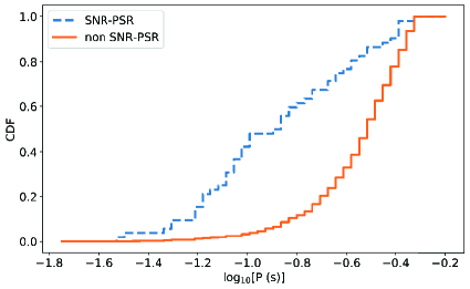
Figure 3: The Cumulative distribution function (CDF) of spin period for SNR-PSRs and non SNR-PSRs. The dashed (solid) line stands for SNR-PSRs (non SNR-PSRs).

In order to see whether the two groups of samples of SNR-PSRs and non SNR-PSRs hold the same distribution, we draw the CDF curves in Figure 3, where the two curves are conspicuously separated to each other. To show the difference of the two samples more quantitatively, we apply the K-S test and M-W-W test, and the p-values of these two tests are as low as $1.98\times 10^{-12}$ and $5.85\times 10^{-13}$. The very low p-values indicate that the distributions of the two samples should have the different origins. Therefore, with the results of two CDF curves and p-values, we believe that the two samples may come from the different statistical distributions. The further test results for the other parameters are shown in Appendix B.

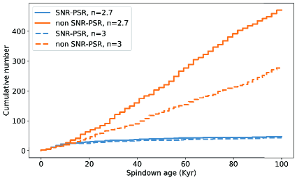
Figure 4: The cumulative number distribution of SNR-PSRs and non SNR-PSRs in different ages. The blue (orange) solid lines stand for SNR-PSRs (non SNR-PSRs) under n=2.7, and dashed lines stand for the cases of n=3.

Next, we draw a cumulative number distribution (Figure 4) for the different ages that are estimated by Eq.(2). Interestingly, for the age less than $\sim$ 10 Kyr the two curves of SNR-PSRs and non SNR-PSRs coincide together, however, after $\rm 10-20\,Kyr$, the two curves are drifted away. The cumulative number ratio, expressed as $N_{snr}/N_{nsnr}$, for the two samples with the different ages probably can infer a fact that the two samples hold the different origins.

In order to see the variation of this ratio between two samples more intuitively, we plot the different ratio values from the age of 5 Kyr to 100 Kyr in Figure 5. We find that, before the age of 25 Kyr, we obtain 5 ratio points for n=2.7 and n=3. While, from 25 Kyr to 100 Kyr, only 2 ratio points are obtained because of the inadequate data. From the data point of these ratio values, we obtain that the number ratio between SNR-PSR and non SNR-PSR is close to unity at the age of $\sim$ 10 Kyr. However, after $\rm 10-20\,Kyr$, there exists a sharp decline in the ratio values. Meanwhile, for the ratio value after $\sim$ 10 Kyr, with n=2.7 (n=3), we obtain a relation between the ratio and the age $\mathcal{\phi}_{2.7}=1.1(t/10kyr)^{-1.01}$ ($\mathcal{\phi}_{3}=1.2(t/10kyr)^{-0.91}$) and goodness of fit $\mathcal{R}_{2.7}^{2}=0.998$ ($\mathcal{R}_{3}^{2}=0.996$), as described in figure 5.

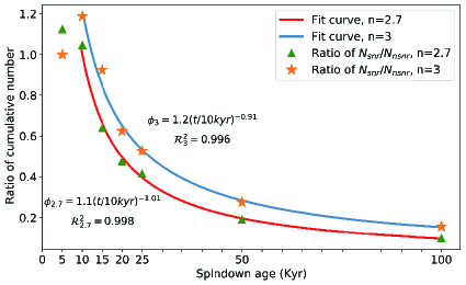
Figure 5: The evolution diagram of cumulative number ratio between SNR-PSRs ($N_{snr}$) and non SNR-PSRs ($N_{nsnr}$). With n=2.7 (n=3), the orange stars (green triangles) stand for the ratio in different ages, and the solid blue (red) line is the fitting curve of these ratio points.

4 Discussions and Conclusions

On the reasons for a sharp drop of the cumulative number ratio between the SNR-PSRs and non-SNR-PSRs, after $\rm 10-20\,Kyr$, together with the the different distributions, we think that there may exist two ways of birth for radio pulsars. The long aged SNR-PSRs may be involved in the high-energy SNe, whereas the non SNR-PSRs may be related to the low energy cases with short duration. For high-mass stars, their SNRs may survive longer time. Correspondingly, the low-energy SNe may be involved in the explosions of the low-mass progenitor stars, in which the SNRs may last a shorter duration.

However, can the effect of decline in cumulative number ratio is caused by the age difference? For example, Leahy, Ranasinghe, & Gelowitz (2020) analysed a 15-Galactic-SNR sample with the best-fit mean energy of $\rm 2.7\times 10^{50}\,erg$, and they concluded that SNRs become incomplete and hard to identify after 30 Kyr. In order to discuss this question more clearly, we need to test for samples with the different spindown ages. According to Figures 4 and 5, the two curves are separated after about $\rm 10-20\,Kyr$ for various braking index. So, we can take 10 Kyr as the critical boundary and divide SNR-PSRs and non SNR-PSRs into two groups by the ages of less and greater than 10 Kyr. For the pulsar ages less than 10 Kyr, the $P$ distributions of SNR-PSRs and non SNR-PSRs are same, while their $\dot{P}$ distributions are different. However, for the pulsar ages more than 10 Kyr, both distributions of $P$ and $\dot{P}$ are different (details in Appendix C). These results may infer that their initial periods are independent on the types of pulsars, but their braking mechanisms are different. The birth of the NSs spin are due to the transfer of angular momentum of progenitors to NSs (Lyne & Graham-Smith 2012), then the energy of SN explosions might little effect on their spin periods. Meanwhile, the difference in $\dot{P}$ will affect the evolution of $P$, resulting in a different distribution of $P$ after 10 Kyr. The above evidence support that their intrinsic differences may lead to different distribution among SNR-PSRs and non SNR-PSRs. Specifically, when radio pulsars are just born, the differences of progenitor mass or explosion energy may create differences in the two groups. The effect of age is to amplify the differences during the evolution, which origin from different initial $\dot{P}$. Thus, this indicates that the differences between SNR-PSRs and non SNR-PSRs in Figures 3, 4, and 5 are more likely to be caused by multiple reasons, rather than only an age difference. The reasons may include different neutron star generation mechanisms and evolution over time.

We need to emphasize that the duration of $\rm 10-20\,Kyr$ is not a strict time, but a statistical value. The result based on SNR evolutionary models (Leahy, Ranasinghe, & Gelowitz 2020) may be slightly different from our result. Although our results ($\rm 10-20\,Kyr$) are not completely the same with their (30 Kyr), at least it shows a life time boundary of two type SNRs, no matter from the perspectives of pulsars in radio and SNRs in X-ray. It can be inferred from this boundary that two types of pulsars generated by two types of SNRs can be roughly distinguished. Therefore, the cumulative number ratio of $\sim 1$ at $\sim$ 10 Kyr may represent the ratio of these two kinds of pulsar production, that is

$$\begin{split}\psi=\frac{N_{snr}}{N_{nsnr}}\sim\frac{N_{high-energy}}{N_{low-energy}}\sim\frac{N_{high-mass}}{N_{low-mass}}\sim 1,\end{split}$$ (3)

where $N_{snr}$ ($N_{nsnr}$), $N_{high-energy}$ ($N_{low-energy}$) and $N_{high-mass}$ ($N_{low-mass}$) represent the numbers of SNR-PSRs (non SNR-PSRs), high (low)energy SNe, and high (low) mass stars. Specifically for the Crab pulsar, it may born from a low-energy SN ($\sim\rm 10^{50}\,erg$) and low-mass progenitor star (Yang & Chevalier 2015). However, the earlier view believed that the Crab Nebula has a more extended remnant (Chevalier 1977), which indicates a higher energy ($\sim\rm 10^{51}\,erg$). Although no medium have been detected in the surrounding area at radio or X-ray band (Frail et al. 1995; Seward, Gorenstein, & Smith 2006), it also reminds us that total energy of the Crab Nebula is still an open question.

The mass range of the progenitor stars for NS formations approximately lies in $\rm 8-25\,M_{\odot}$ (Arnett & Schramm 1973; Miyaji et al. 1980; Heger et al. 2003). If we consider the initial mass function (IMF) by Salpeter, described as $\rm dN/dm=\xi_{0}m^{-2.35}$ (Salpeter 1955), where m is star mass in $\rm M_{\odot}$ units and $\rm\xi_{0}$ is normalization coefficient, to calculate the boundary mass value for the high and low stellar masses, corresponding to the SNR-PSRs and non SNR-PSRs, we obtain this critical mass to be be at $\rm\sim 12\,M_{\odot}$, as shown in Figure 6. So, the SNRs by the low-mass ($\rm 8-12\,M_{\odot}$) progenitor stars may be survived with a shorter time around $\rm 10-20\,Kyr$ (Braun, Goss, & Lyne 1989), which may be a reason for the lots of young pulsars without SNRs.

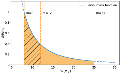
Figure 6: The mass distribution of stars for SNR-PSRs and non SNR-PSRs according to initial mass function (IMF) (Salpeter 1955). The blue solid line is the curve of IMF. The left and right orange solid lines are lower ($\rm 8\,M_{\odot}$) and upper ($\rm 25\,M_{\odot}$) mass limit for NS production, respectively. The area of $\rm 8-12\,M_{\odot}$ ($\rm 12-25\,M_{\odot}$) stands for the progenitor stars for non-SNR-PSRs (SNR-PSRs).

The physical process of these two types of SNe can be described as the iron core collapse and electron capture, and the latter is driven by the neutrino (Janka 2012, 2017). The iron core collapse is the dominant process of high-energy SNe that is generated from high-mass main sequence stars (Heger et al. 2003). The electron capture may be an explanation for the low-energy SNe, while the degenerate oxygen-neon core is collapsed to form the NS(Barkat, Reiss, & Rakavy 1974; Nomoto 1984), and the mass range of these progenitor stars is about $\rm\sim 8-10\,M_{\odot}$ (Nomoto & Leung 2017; Leung, Nomoto, & Suzuki 2020).

Moreover, the mass boundary values given by some researchers are similar to ours, as $\rm\sim 12\,M_{\odot}$ (Sugimoto & Nomoto 1980; Miyaji et al. 1980). However Nomoto (1984) and Heger et al. (2003) obtained the boundary mass as $\rm\sim 10\,M_{\odot}$. It is remarked that our result is based on a statistics, but not a numerical calculation result from a stellar theoretical model. In addition, because of less pulsar samples at the young age ($<$10 Kyr), the ratio in Eq.(3) may be biased, which will directly affect the mass boundary.

Finally, the main conclusions are summarized below: The 52 SNR-PSRs and 630 non SNR-PSRs have been tested (K-S and M-W-W) and analyzed (cumulative number ratio), implying different $\dot{P}$ and other properties for the two sets, perhaps associated with the different mass ranges of their progenitor masses for SN explosions. The critical mass of different progenitor stars is estimated by the Salpeter initial mass function, obtained as $\rm 12\,M_{\odot}$. The low-mass stars (high-mass) with $\rm\sim 8-12\,M_{\odot}$ ($\rm\sim 12-25\,M_{\odot}$) will generate the low-energy (high-energy) SNe in the shorter (longer) SNR duration of about $\rm<10-20\,Kyr$ ($\rm>10-20\,Kyr$). These conjectures can explain why many young radio pulsars are not seen inside SNRs. In the future, with the observations by FAST (Li et al. 2018) and launch of James Webb Space Telescope (JWST) (Gardner et al. 2006), more fainter and weaker pulsars and SNRs would be discovered, which will present the better constraints on our conclusions.

Data Availability

The data underlying this article are available in the references below: (1) pulsars data are taken from ATNF Pulsar Catalogue, available at https://www.atnf.csiro.au/research/pulsar/psrcat/; (2) SNR data are taken from SNRcat, available at http://snrcat.physics.umanitoba.ca/SNRtable.php.

Appendix A: Derivation of period evolution equation

Energy loss rate of a spin-powered pulsar can be expressed as

$$\begin{split}\dot{E}=\frac{dE}{dt}=\frac{d(I\Omega^{2}/2)}{dt}=-I\Omega\dot{\Omega},\end{split}$$ (4)

where $E$ is total energy of pulsar, $\dot{E}$ is energy loss rate, $\Omega$ is spin angular velocity, $\dot{\Omega}$ is rate of spin angular velocity, and $I$ is moment of inertia. When the pulsar kinetic energy and the radiation energy loss rate are equal, then there is

$$\begin{split}I\Omega\dot{\Omega}=K\Omega^{\rm n+1},\end{split}$$ (5)

where $K$ is coefficient, We combined with $\Omega=2\pi/P$ and integrate both sides of above equation,

$$\begin{split}\int_{P_{0}}^{P(t)}P^{\rm n-2}d\dot{P}=\int_{0}^{t}-\frac{K}{I}(2\pi)^{\rm n-1}dt.\end{split}$$ (6)

With assuming that the rate has been constant since pulsar birth, then spin period evolution equation can be written as

$$\begin{split}P(t)=\left[({\rm n-1})P_{0}^{\rm n-2}\dot{P}_{0}t+P_{0}^{\rm n-1}\right]^{1/(\rm n-1)}.\end{split}$$ (7)

In the above equation, $P_{0}$ and $\dot{P}_{0}$ is spin period and rate at present, respectively. The spindown age of pulsar is $\tau=P/[({\rm n-1})\dot{P}]$, which is different with characteristic age $\tau_{c}=P/(\rm 2\dot{P})$. Then Eq.(7) can be rewritten as

$$\begin{split}P(t)=P_{0}\left(\frac{t}{\tau}_{0}+1\right)^{1/(\rm n-1)}.\end{split}$$ (8)

When $t\gg\tau_{0}$, the equation can be simplified to

$$\begin{split}P(t)\approx P_{0}\left(\frac{t}{\tau}_{0}\right)^{1/(\rm n-1)}.\end{split}$$ (9)

Appendix B: Further tests of derivative of spin period, B-field and energy loss rate

If the origin of pulsars that with or without SNRs are indeed different, then the distribution of other physical parameters should also be different. Here we discuss the derivative of spin period ($\dot{P}$), B-field strength ($B$ with n=3) and energy loss rate ($\dot{E}$) by applying K-S and M-W-W tests, and the results are shown in Table 2, and the CDFs are shown in Figure 7, 8 and 9, where the distributions for two samples of SNR-PSRs and non SNR-PSRs are different respect to these three parameters. For $\dot{P}$, the two groups with the different ages share the significantly different distributions, which implies that the braking mechanisms of them perhaps are different. The physical parameter distributions of two samples are quite different, which possibly could be ascribed to the different origins of radio pulsars.

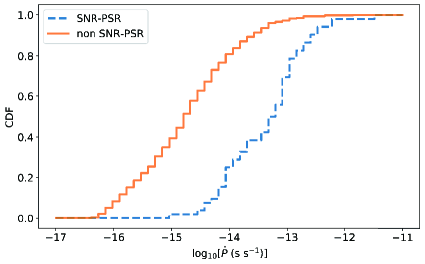
Figure 7: The Cumulative distribution function (CDF) of derivative of spin period ($\dot{P}$) of SNR-PSRs and non SNR-PSRs. The dashed line is for SNR-PSRs, and the solid line is for non SNR-PSRs.

Figure 8: The Cumulative distribution function (CDF) of surface magnetic field strength ($B$ with n=3) of SNR-PSRs and non SNR-PSRs. The dashed line is for SNR-PSRs, and the solid line is for non SNR-PSRs.

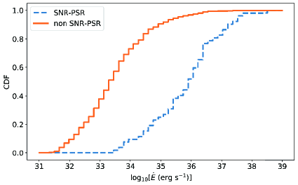
Figure 9: The Cumulative distribution function (CDF) of spin down energy loss rate ($\dot{E}$) of SNR-PSRs and non SNR-PSRs. The dashed line is for SNR-PSRs, and the solid line is for non SNR-PSRs.

Table 2: P-values of K-S and M-W-W test for different parameters

Physical parametersa	K-S test	M-W-W test
$P$	$1.98\times 10^{-12}$	$5.85\times 10^{-13}$
$\dot{P}$	$1.55\times 10^{-15}$	$6.41\times 10^{-21}$
$B$	$3.24\times 10^{-11}$	$2.12\times 10^{-14}$
$\dot{E}$	$1.55\times 10^{-15}$	$4.33\times 10^{-24}$

^a $P$ is spin period, $\dot{P}$ is derivative of spin period, $B$ is surface magnetic field strength, and $\dot{E}$ is energy loss rate of radio pulsars.

Appendix C: Tests of spin period and its derivative with the different ages

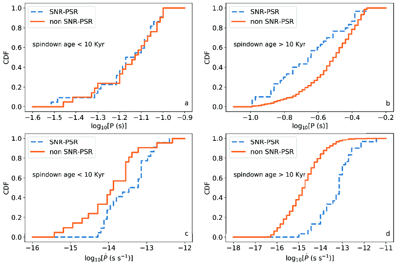
Figure 10: The Cumulative distribution function (CDF) of spin period ($P$) and its derivative ($\dot{P}$) of SNR-PSRs and non SNR-PSRs with the spindown ages of less and over than 10 Kyr. The sub-figures of a and b are CDF of $P$, and the sub-figures of c and d are CDF of $\dot{P}$. For all sub-figures, the dashed line represents SNR-PSRs, and the solid line is for non SNR-PSRs. The text in each sub-figure shows their age ranges.

Table 3: P-values of K-S and M-W-W test for $P$ and $\dot{P}$ with different ages

Physical parametersa	Spindown age	K-S test	M-W-W test
$P$	¡10 Kyr	0.99	0.85
	¿10 Kyr	$2.75\times 10^{-3}$	$4.83\times 10^{-4}$
$\dot{P}$	¡10 Kyr	$3.41\times 10^{-2}$	$5.34\times 10^{-2}$b
	¿10 Kyr	$4.38\times 10^{-13}$	$1.64\times 10^{-13}$

^a $P$ is spin period, $\dot{P}$ is derivative of spin period.

^b Although this value is slightly larger than 0.05, it may also imply that the two samples have different statistical distributions at a 90% probability (e.g. if p-value is less than 0.1, it indicates that this test rejects the null hypothesis that the two samples have the same distribution at 10% significance level).

In this part, we plot distributions of $P$ with different age ranges of less and over than 10 Kyr in Figure 10 (subplots a & b). After K-S and M-W-W tests (Table 3), we find that when the spindown age is less than 10 Kyr the $P$ distributons of SNR-PSRs and non SNR-PSRs are the same. But the distributions of $P$ after 10 Kyr are different. Meanwhile, distributions of $\dot{P}$ are also tested with the same age ranges as that of $P$ (less and more than 10 Kyr) in Figure 10 (subplots c & d). Interestingly, regardless of the age ranges, the $\dot{P}$ distributions are different under K-S tests in Table 3. The possible physical explanation is that although the initial $P$ distribution is the same, the initial $\dot{P}$ is different, which makes pulsars no longer have the same $P$ distribution after evolution over 10 Kyr. Thus, the above evidence supports that the differences between the SNR-PSRs and non SNR-PSRs are possibly the result of a combined effect of different mechanisms and evolution, but not just caused by age difference.

References

- Arnett & Schramm (1973) Arnett W. D., Schramm D. N., 1973, ApJL, 184, L47.
- Barkat, Reiss, & Rakavy (1974) Barkat Z., Reiss Y., Rakavy G., 1974, ApJL, 193, L21.
- Bhattacharya & van den Heuvel (1991) Bhattacharya D., van den Heuvel E. P. J., 1991, PhR, 203, 1.
- Braun, Goss, & Lyne (1989) Braun R., Goss W. M., Lyne A. G., 1989, ApJ, 340, 355.
- Čadež et al. (2016) Čadež A., Zampieri L., Barbieri C., Calvani M., Naletto G., Barbieri M., Ponikvar D., 2016, A&A, 587, A99.
- Camilo, Thorsett, & Kulkarni (1994) Camilo F., Thorsett S. E., Kulkarni S. R., 1994, ApJL, 421, L15.
- Chevalier (1977) Chevalier R. A., 1977, ASSL, 53.
- Cui et al. (2021) Cui X.-H., Zhang C.-M., Wang S.-Q., Zhang J.-W., Li D., Peng B., Zhu W.-W., et al., 2021, MNRAS, 500, 3275.
- Duncan & Thompson (1992) Duncan R. C., Thompson C., 1992, ApJL, 392, L9.
- Esposito, Rea, & Israel (2021) Esposito P., Rea N., Israel G. L., 2021, ASSL, 97.
- Ferrand & Safi-Harb (2012) Ferrand G., Safi-Harb S., 2012, AdSpR, 49, 1313.
- Ferrario & Wickramasinghe (2008) Ferrario L., Wickramasinghe D., 2008, MNRAS, 389, L66.
- Frail, Goss, & Whiteoak (1994) Frail D. A., Goss W. M., Whiteoak J. B. Z., 1994, ApJ, 437, 781.
- Frail et al. (1995) Frail D. A., Kassim N. E., Cornwell T. J., Goss W. M., 1995, ApJL, 454, L129.
- Gaensler & Johnston (1995) Gaensler B. M., Johnston S., 1995, MNRAS, 277, 1243.
- Gaensler & Slane (2006) Gaensler B. M., Slane P. O., 2006, ARA&A, 44, 17.
- Gardner et al. (2006) Gardner J. P., Mather J. C., Clampin M., Doyon R., Greenhouse M. A., Hammel H. B., Hutchings J. B., et al., 2006, SSRv, 123, 485.
- Goldreich & Julian (1969) Goldreich P., Julian W. H., 1969, ApJ, 157, 869.
- Gotthelf, Halpern, & Alford (2013) Gotthelf E. V., Halpern J. P., Alford J., 2013, ApJ, 765, 58.
- Greco et al. (2021) Greco E., Miceli M., Orlando S., Olmi B., Bocchino F., Nagataki S., Ono M., et al., 2021, ApJL, 908, L45.
- Halpern & Gotthelf (2010) Halpern J. P., Gotthelf E. V., 2010, ApJ, 710, 941.
- Han et al. (2021) Han J. L., Wang C., Wang P. F., Wang T., Zhou D. J., Sun J.-H., Yan Y., et al., 2021, RAA, 21, 107.
- Heger et al. (2003) Heger A., Fryer C. L., Woosley S. E., Langer N., Hartmann D. H., 2003, ApJ, 591, 288.
- Igoshev & Popov (2013) Igoshev A. P., Popov S. B., 2013, MNRAS, 432, 967.
- Janka (2012) Janka H.-T., 2012, ARNPS, 62, 407.
- Janka (2017) Janka H.-T., 2017, hsn..book, 1095.
- Johnston & Galloway (1999) Johnston S., Galloway D., 1999, MNRAS, 306, L50.
- Kaspi et al. (2001) Kaspi V. M., Roberts M. E., Vasisht G., Gotthelf E. V., Pivovaroff M., Kawai N., 2001, ApJ, 560, 371.
- Kaspi & Beloborodov (2017) Kaspi V. M., Beloborodov A. M., 2017, ARA&A, 55, 261.
- Knigge, Coe, & Podsiadlowski (2011) Knigge C., Coe M. J., Podsiadlowski P., 2011, Natur, 479, 372.
- Kou & Tong (2015) Kou F. F., Tong H., 2015, MNRAS, 450, 1990.
- Kramer et al. (2006) Kramer M., Lyne A. G., O’Brien J. T., Jordan C. A., Lorimer D. R., 2006, Sci, 312, 549.
- Lai (1996) Lai D., 1996, ApJL, 466, L35.
- Large, Vaughan, & Mills (1968) Large M. I., Vaughan A. E., Mills B. Y., 1968, Natur, 220, 340.
- Leahy (2017) Leahy D. A., 2017, ApJ, 837, 36.
- Leahy, Ranasinghe, & Gelowitz (2020) Leahy D. A., Ranasinghe S., Gelowitz M., 2020, ApJS, 248, 16.
- Leung, Nomoto, & Suzuki (2020) Leung S.-C., Nomoto K., Suzuki T., 2020, ApJ, 889, 34.
- Li et al. (2018) Li D., Wang P., Qian L., Krco M., Jiang P., Yue Y., Jin C., et al., 2018, IMMag, 19, 112.
- Lorimer et al. (1993) Lorimer D. R., Bailes M., Dewey R. J., Harrison P. A., 1993, MNRAS, 263, 403.
- Lorimer (2004) Lorimer D. R., 2004, IAUS, 218, 105
- Lorimer (2008) Lorimer D. R., 2008, LRR, 11, 8.
- Lorimer & Kramer (2012) Lorimer D. R., Kramer M., 2012, hpa..book
- Lyne, Manchester, & Taylor (1985) Lyne A. G., Manchester R. N., Taylor J. H., 1985, MNRAS, 213, 613.
- Lyne & Graham-Smith (2012) Lyne A., Graham-Smith F., 2012, puas.book
- Lyne et al. (2015) Lyne A. G., Jordan C. A., Graham-Smith F., Espinoza C. M., Stappers B. W., Weltevrede P., 2015, MNRAS, 446, 857.
- Malov (2021) Malov I. F., 2021, MNRAS, 502, 809.
- Manchester (1987) Manchester R. N., 1987, A&A, 171, 205
- Manchester et al. (2005) Manchester R. N., Hobbs G. B., Teoh A., Hobbs M., 2005, AJ, 129, 1993.
- McLaughlin et al. (2006) McLaughlin M. A., Lyne A. G., Lorimer D. R., Kramer M., Faulkner A. J., Manchester R. N., Cordes J. M., et al., 2006, Natur, 439, 817.
- Miyaji et al. (1980) Miyaji S., Nomoto K., Yokoi K., Sugimoto D., 1980, PASJ, 32, 303
- Narayan & Schaudt (1988) Narayan R., Schaudt K. J., 1988, ApJL, 325, L43.
- Nomoto (1984) Nomoto K., 1984, ApJ, 277, 791.
- Nomoto & Leung (2017) Nomoto K., Leung S.-C., 2017, hsn..book, 483.
- Morello et al. (2020) Morello V., Keane E. F., Enoto T., Guillot S., Ho W. C. G., Jameson A., Kramer M., et al., 2020, MNRAS, 493, 1165.
- Olausen & Kaspi (2014) Olausen S. A., Kaspi V. M., 2014, ApJS, 212, 6.
- Page et al. (2020) Page D., Beznogov M. V., Garibay I., Lattimer J. M., Prakash M., Janka H.-T., 2020, ApJ, 898, 125.
- Popov & Turolla (2012) Popov S. B., Turolla R., 2012, Ap&SS, 341, 457.
- Radhakrishnan & Srinivasan (1980) Radhakrishnan V., Srinivasan G., 1980, JApA, 1, 25.
- Salpeter (1955) Salpeter E. E., 1955, ApJ, 121, 161.
- Seward, Gorenstein, & Smith (2006) Seward F. D., Gorenstein P., Smith R. K., 2006, ApJ, 636, 873.
- Shapiro & Teukolsky (1983) Shapiro S. L., Teukolsky S. A., 1983, bhwd.book
- Soker (2021) Soker N., 2021, NewA, 84, 101548.
- Srinivasan, Bhattacharya, & Dwarakanath (1984) Srinivasan G., Bhattacharya D., Dwarakanath K. S., 1984, JApA, 5, 403.
- Staelin & Reifenstein (1968) Staelin D. H., Reifenstein E. C., 1968, Sci, 162, 1481.
- Stollman (1987) Stollman G. M., 1987, A&A, 178, 143
- Sugimoto & Nomoto (1980) Sugimoto D., Nomoto K., 1980, SSRv, 25, 155.
- Tan et al. (2018) Tan C. M., Bassa C. G., Cooper S., Dijkema T. J., Esposito P., Hessels J. W. T., Kondratiev V. I., et al., 2018, ApJ, 866, 54.
- Taylor & Manchester (1977) Taylor J. H., Manchester R. N., 1977, ApJ, 215, 885.
- Tian & Leahy (2006) Tian W. W., Leahy D. A., 2006, A&A, 455, 1053.
- Yang & Chevalier (2015) Yang H., Chevalier R. A., 2015, ApJ, 806, 153.
- Yang et al. (2019) Yang Y.-Y., Zhang C.-M., Li D., Chen L., Linghu R.-F., Zhi Q.-J., 2019, PASP, 131, 064201.
- Ye et al. (2019) Ye C.-Q., Wang D.-H., Zhang C.-M., Diao Z.-Q., 2019, Ap&SS, 364, 198. doi:10.1007/s10509-019-3690-1
- Zhang & Kojima (2006) Zhang C. M., Kojima Y., 2006, MNRAS, 366, 137.