ebnm: An R Package for Solving the Empirical Bayes Normal Means Problem Using a Variety of Prior Families

Jason Willwerscheid, Peter Carbonetto, and Matthew Stephens ebnm: An R Package for Solving the Empirical Bayes Normal Means Problem ebnm: Empirical Bayes Normal Means in R The empirical Bayes normal means (EBNM) model is important to many areas of statistics, including (but not limited to) multiple testing, wavelet denoising, multiple linear regression, and matrix factorization. There are several existing software packages that can fit EBNM models under different prior assumptions and using different algorithms; however, the differences across interfaces complicate direct comparisons. Further, a number of important prior assumptions do not yet have implementations. Motivated by these issues, we developed the R package ebnm which provides a unified interface for efficiently fitting EBNM models using a variety of prior assumptions, including nonparametric approaches. In some cases, we incorporated existing implementations into ebnm; in others, we implemented new fitting procedures with a focus on speed and numerical stability. To demonstrate the capabilities of the unified interface, we compare results using different prior assumptions in two extended examples: the shrinkage estimation of baseball statistics; and the matrix factorization of genetics data (via the new R package flashier). In summary, ebnm is a convenient and comprehensive package for performing EBNM analyses under a wide range of prior assumptions. empirical Bayes, normal means, shrinkage estimation, mixture models, NPMLE, maximum likelihood empirical Bayes, normal means, shrinkage estimation, mixture models, NPMLE, maximum likelihood Jason Willwerscheid
Department of Mathematics and Computer Science
Providence College
Providence, Rhode Island, United States of America
E-mail:
Peter Carbonetto
Department of Human Genetics and the
Research Computing Center
University of Chicago
Chicago, Illinois, United States of America
E-mail:
Matthew Stephens
Departments of Statistics and Human Genetics
University of Chicago
Chicago, Illinois, United States of America
E-mail:

1 Introduction

Given $n$ observations $x_{i}$ with known standard deviations $s_{i}$, $i=1,\dots,n$, the normal means model (Robbins51; efron1972limiting; Stephens_NewDeal; bhadra2019lasso; Johnstone; lei-thesis) is

$$x_{i}\overset{\text{ind.}}{\sim}\mathcal{N}(\theta_{i},s_{i}^{2}),$$ (1)

with the unknown (true) means $\theta_{i}$ to be estimated. Here and throughout, we use $\mathcal{N}(\mu,\sigma^{2})$ to denote the normal distribution with mean $\mu$ and variance $\sigma^{2}$. The maximum-likelihood estimate of $\theta_{i}$ is, of course, $x_{i}$. The empirical Bayes (EB) approach to inferring $\theta_{i}$ attempts to improve upon the maximum-likelihood estimate by “borrowing information” across observations, exploiting the fact that each observation contains information not only about its respective mean, but also about how the means are collectively distributed (Robbins56; Morris; Efron_Book; Stephens_NewDeal). Specifically, the EB approach assumes that

$$\theta_{i}\overset{\text{ind.}}{\sim}g\in\mathcal{G},$$ (2)

where $g$ is a distribution to be estimated from the data, typically chosen from among some family of distributions $\mathcal{G}$ that is specified in advance. (Note that although $\mathcal{G}$ must be specified in advance, it can be arbitrarily flexible.)

The EB approach therefore involves fitting the model (1–2) by first using all of the observations to estimate $g\in\mathcal{G}$, then using the estimated distribution $\hat{g}$ to compute posteriors for each mean $\theta_{i}$. Commonly, $g$ is estimated via maximum-likelihood, in which case the EB approach consists of the following:

1. Find $\hat{g}\colonequals\operatorname*{argmax}_{g\,\in\,\mathcal{G}}L(g)$, where $L(g)$ denotes the marginal likelihood,

   $$L(g)\colonequals p({\bm{x}}\mid g,{\bm{s}})=\prod_{i=1}^{n}\textstyle\int p(x_{i}\mid\theta_{i},s_{i})\,g(\theta_{i})\,d\theta_{i},$$ (3)

   and we define ${\bm{x}}\colonequals(x_{1},\ldots,x_{n})$, ${\bm{s}}\colonequals(s_{1},\ldots,s_{n})$.

2. Compute posterior distributions

   $$p(\theta_{i}\mid x_{i},s_{i},\hat{g})\propto\hat{g}(\theta_{i})\,p(x_{i}\mid\theta_{i},s_{i})$$ (4)

   and/or summaries (posterior means, variances, etc.).

We refer to this two-step process as “solving the EBNM problem.” The difficulty of both steps depends upon the choice of $\mathcal{G}$.

A large number of software packages have been developed to solve the EBNM problem (we review these packages below). The availability of so many methods, using a range of prior families $\mathcal{G}$, reflects the important role of the EBNM problem in theoretical and applied statistics. Among the many possible applications of the EBNM problem, we mention a few: wavelet denoising (ClydeGeorge; JohnstoneSilverman_Needles; JohnstoneSilverman_Wavelet); multiple testing (Efron_Book; Stephens_NewDeal); analysis of gene expression (deseq2; zhu-2019); multiple linear regression (mr_ash; mukherjee-2023); and matrix factorization (WangStephens).

However, there are important gaps in the existing software. For example, as far as we are aware, no package solves the EBNM problem for one of the simplest cases: when $\mathcal{G}$ is the set of all univariate normal distributions. Nor does any existing package implement the case where $\mathcal{G}$ is the “point-normal” family (the family of all distributions that are a mixture of a point-mass at zero and a zero-centered normal distribution), which arises naturally when the means $\bm{\theta}=(\theta_{1},\ldots,\theta_{n})$ are expected to be sparse. Further, each package has a different interface and outputs, which makes comparisons difficult, as well as making it difficult to develop software packages that build on EBNM methods.

Motivated by these issues, we developed the R package ebnm, which provides a unified interface for efficiently solving the EBNM problem using a wide variety of prior families. For some prior families, we leveraged code from existing packages, writing wrappers to match the unified ebnm interface; for other priors, we implemented new model-fitting algorithms with a mind toward speed and robustness. The end result is a comprehensive and user-friendly package for solving the EBNM problem.

In Section 2, we give a brief history of the EBNM problem and review existing approaches. Section 3 gives an overview of the ebnm package, including the unified interface and the newly implemented prior families. In Section 4, we compare different choices of prior families and illustrate how they can impact performance. Finally, Sections 5 and LABEL:section:ebnm_snmf demonstrate usage of the ebnm package in two real-data applications: an analysis of weighted on-based averages for Major League Baseball players; and an exploration of EBNM-based matrix factorization methods that can identify biological patterns underlying multi-tissue gene expression data.

2 Background on the EBNM problem, and existing software

Here we review existing approaches to the EBNM problem within a common modeling framework.

2.1 Normal priors

Stein famously discovered that under quadratic loss, the maximum-likelihood estimate, $\hat{\theta}_{i}=x_{i}$, $i=1,\ldots,n$, is an inadmissible solution to the homoskedastic normal means problem

$$x_{i}\overset{\text{ind.}}{\sim}\mathcal{N}(\theta_{i},s^{2}),\qquad i=1,\ldots,n,$$ (5)

when $n\geq 3$. JamesStein subsequently gave an explicit formula for a shrinkage estimator that dominates the MLE. As EfronMorris showed, a lightly modified version of the James-Stein estimator can be derived via an EB approach that assumes

$$\theta_{i}\overset{\text{ind.}}{\sim}g\in\mathcal{G},$$ (6)

where the prior family $\mathcal{G}$ is taken to be the family of zero-mean normal distributions

$$\mathcal{G}_{\text{norm0}}\colonequals\big{\{}g:g\sim\mathcal{N}(0,\sigma^{2}),\,\sigma^{2}\geq 0\big{\}}.$$ (7)

In many applications, the mean of the $\theta_{i}$’s may be non-zero, and so a natural generalization takes $\mathcal{G}$ to be the family of normal distributions

$$\mathcal{G}_{\text{norm}}\colonequals\big{\{}g:g\sim\mathcal{N}(\mu,\sigma^{2}),\,\sigma^{2}\geq 0\mbox{ and }\mu\in\mathbb{R}\big{\}}.$$ (8)

Estimating $g\in\mathcal{G}_{\text{norm}}$ reduces to estimating $\sigma^{2}$ and $\mu$. For the homoskedastic case (5), the maximum-likelihood estimates have simple, closed-form solutions:

$$\hat{\mu} =\frac{1}{n}\sum_{i=1}^{n}x_{i},$$ (9)

$$\hat{\sigma}^{2} =\max\bigg{\{}0,\frac{1}{n}\sum_{i=1}^{n}(x_{i}-\hat{\mu})^{2}-s^{2}\bigg{\}}.$$ (10)

When $\mu$ is fixed at zero, this solution is similar to the one implied by the positive-part James-Stein estimator, with the difference that it divides $\sum_{i=1}^{n}x_{i}^{2}$ by $n$ rather than by $n-2$ (EfronMorris). For the heteroskedastic case (1), the likelihood $L(\mu,\sigma^{2})$ has a closed form but must be maximized numerically. In both the homoskedastic and heteroskedastic cases, the posteriors (4) are normal distributions and are available analytically. Surprisingly, we were unable to find an existing software package that handled these cases.

2.2 Other priors

Although the normal prior family has some advantages, in practice it is limiting, and so more flexible priors are usually preferred. For example, when $\bm{\theta}$ may be sparse, we might like the prior to be able to capture this sparsity. One common approach is to use a “spike-and-slab” prior; that is, a mixture consisting of two components, one a point-mass at zero (the “spike”) and the other (the “slab”) belonging to some family of continuous distributions, often symmetric and centered at zero. A common choice is the “point-normal” family,

$$\mathcal{G}_{\text{pn}}\colonequals\big{\{}g:g\sim\pi_{0}\delta_{0}+(1-\pi_{0})\mathcal{N}(0,\sigma^{2}),\,0\leq\pi_{0}\leq 1,\,\sigma^{2}>0\big{\}}.$$ (11)

With this choice, estimating $g$ reduces to estimating two parameters, $\pi_{0}$ and $\sigma$. Similar to the normal prior, the likelihood for the point-normal has a closed form, and standard numerical optimization methods can be used to efficiently find the maximum-likelihood solution. (Since the likelihood as a function of $\pi_{0}$ and $\sigma$ is not convex, there may be multiple “locally optimal” solutions, and typically the numerical optimization method is only guaranteed to find a locally optimal solution.) Given the estimate $\hat{g}\in\mathcal{G}_{\text{pn}}$, the posteriors (4) are mixtures of a point-mass at zero and a normal distribution, and are available analytically. Again, to our surprise, we were unable to find a software implementation of EBNM that uses the point-normal prior family, and so we have provided our own implementation in the ebnm package.

While a normal slab is most popular, other choices are possible. JohnstoneSilverman_Wavelet showed that replacing the normal slab with a “heavy-tailed” distribution is guaranteed to improve accuracy. Their EbayesThresh software, available in R and S-PLUS (EbayesThresh_paper), implements two such priors: the point-Laplace prior,

$$\mathcal{G}_{\text{pl}}\colonequals\big{\{}g:g\sim\pi_{0}\delta_{0}+(1-\pi_{0})\text{Laplace}(a),\,0\leq\pi_{0}\leq 1,\,a\geq 0\big{\}},$$ (12)

and a family of priors in which the slab has “Cauchy-like” tails. Again, the optimization problem for both of these priors is non-convex, and local solutions can be found using numerical methods.

Another parametric prior that is well-suited for capturing sparse signals is the horseshoe prior (Horseshoe), which models sparsity by having appreciable mass near zero rather than exactly at zero. The R package horseshoe (Horseshoe_Package) includes an implementation that solves the homoskedastic EBNM problem with $\mathcal{G}$ the family of horseshoe distributions. See bhadra2019lasso for a review of other implementations of the horseshoe prior and related packages.

2.3 Nonparametric approaches

The estimate of $g$ when $\mathcal{G}$ is the family of all distributions is called the nonparametric maximum-likelihood estimate (NPMLE). Nonparametric approaches have been studied for nearly as long as parametric approaches (KieferWolfowitz; Laird; Lindsay; JiangZhang; KoenkerMizera; DickerZhao). In practice, most nonparametric methods approximate $\mathcal{G}=\mathcal{G}_{\text{npmle}}$ by a dense but finite mixture of point masses,

$$\tilde{\mathcal{G}}_{\text{npmle}}\colonequals\bigg{\{}g:g\sim\sum_{k=1}^{K}\pi_{k}\delta_{\mu_{k}}\,\bigg{|}\,\pi_{1},\ldots,\pi_{K}\geq 0,\,\sum_{k=1}^{K}\pi_{k}=1\bigg{\}}$$ (13)

where $\mu_{1},\dots,\mu_{K}$ is a fixed, dense grid of values along the real line spanning the range of the observations. Estimating $g\in\tilde{\mathcal{G}}_{\text{npmle}}$ amounts to solving the following constrained optimization problem:

$$\begin{array}[]{ll}\mbox{maximize}&\mathbf{L}\bm{\pi}\\ \mbox{subject to}&\bm{0}\preceq\bm{\pi}\preceq\bm{1}_{K}\\ &\bm{\pi}^{T}\bm{1}_{K}=1,\end{array}$$ (14)

where ${\bm{\pi}}\colonequals(\pi_{1},\ldots,\pi_{K})^{T}$, ${\bm{1}}_{K}$ is a column vector of ones of length $K$, and $\mathbf{L}\in\mathbb{R}^{n\times K}$ is the matrix with entries $\ell_{ik}=\mathcal{N}(x_{i};\mu_{k},\sigma_{i}^{2})$. This is a convex optimization problem (KoenkerMizera); the R package REBayes (KoenkerGu) implements an efficient solution based on interior point optimization methods (mosek). See MixSQP and ZhangCui for other approaches to solving this optimization problem.

Although the fully nonparametric approach is the most flexible, the estimates of $g$ are discrete distributions, which also leads to discrete posteriors (4) (Laird). The posterior mean from a discrete prior may be perfectly adequate for point estimation even when interval estimates perform less well; see, for example, KoenkerVinaigrette. However, in some cases the lack of smoothness of the estimate can be an issue. The R package deconvolveR (NarasimhanEfron) uses a natural spline basis to obtain a smoothed nonparametric estimate of $g$. This approach can outperform the NPMLE in certain respects when the true prior is smooth (KoenkerVinaigrette).

2.4 Constrained nonparametric approaches

Constrained nonparametric approaches can also produce smoother and arguably more plausible estimates of $g$. For example, in the context of multiple testing, Stephens_NewDeal suggested that the set of all distributions that are unimodal at zero is a reasonable choice for $\mathcal{G}$ in many settings. If it is reasonable to assume that the prior $g$ is symmetric, one can instead take $\mathcal{G}$ to be the family of scale mixtures of normals,

$$\mathcal{G}_{\text{smn}}\colonequals\textstyle\big{\{}g:g\sim\int_{0}^{\infty}\mathcal{N}(0,\sigma^{2})\,dh(\sigma^{2})\text{ for some }h\big{\}},$$ (15)

or, for slightly more flexibility, the family of all symmetric distributions that are unimodal at zero, which can be represented by scale mixtures of uniform distributions,

$$\mathcal{G}_{\text{symm-u}}\colonequals\textstyle\big{\{}g:g\sim\int_{0}^{\infty}\mathrm{Unif}[-a,a]\,dh\left(a\right)\text{ for some }h\big{\}}.$$ (16)

When these families are approximated by finite mixtures, estimating $g$ reduces to the same convex optimization problem (14) that arises from the NPMLE, and can again be solved using fast algorithms for convex optimization. This approach is implemented in the R package ashr (ashr), which, by default, uses mixsqp (MixSQP) to solve the optimization problem (14).

2.5 Flexibility of the prior families

Some prior families are more flexible than others; for example, any normal prior is also a point-normal prior, but most point-normal priors cannot be recovered as a normal prior. More broadly, we have that

$$\mathcal{G}_{\text{norm0}}\subset\mathcal{G}_{\text{pn}}\subset\mathcal{G}_{\text{smn}}\subset\mathcal{G}_{\text{symm-u}}\subset\mathcal{G}_{\text{npmle}}.$$ (17)

In words, the family of zero-mean normals $\mathcal{G}_{\text{norm0}}$ is a subset of the family of point-normals $\mathcal{G}_{\text{pn}}$, which is in turn a subset of the family of scale mixtures of normals $\mathcal{G}_{\text{smn}}$. $\mathcal{G}_{\text{smn}}$ is a subset of the family of symmetric unimodal priors $\mathcal{G}_{\text{symm-u}}$, and $\mathcal{G}_{\text{symm-u}}$ is a subset of the nonparametric family of all distributions $\mathcal{G}_{\text{npmle}}$. Additionally, the families of point-Laplace priors $\mathcal{G}_{\text{pl}}$ and horseshoe priors $\mathcal{G}_{\text{horseshoe}}$ are contained in $\mathcal{G}_{\text{smn}}$, and $\mathcal{G}_{\text{deconvolver}}\subseteq\mathcal{G}_{\text{npmle}}$.

More flexibility is in general better, but only up to a point since a prior family that is overly flexible can have the potential to “overfit” (hastie2009elements). Ideally, one would like to select the prior family in a “data-driven” way; that is, use the data to help identify an appropriate prior family. The ebnm package faciliates this process by making it easy to compare prior families within a unified interface. (We caution, however, that ebnm does not implement formal testing.)

3 The ebnm package: implementation and usage

The ebnm package offers a unified interface for solving the EBNM problem under a wide range of prior assumptions. In addition to making available previously existing implementations via a shared interface, the package provides new implementations for several simple but useful prior families that, to our knowledge, have not previously been implemented (e.g., the normal and point-normal prior families).

3.1 The ebnm() function

The ebnm() function is the main interface to the EBNM methods. It has the following input arguments, which, apart from the first argument x, are all optional:

• x: The vector of observations, ${\bm{x}}=\{x_{1},\ldots,x_{n}\}$.

• s: The vector of standard errors, ${\bm{s}}=\{s_{1},\ldots,s_{n}\}$. (s may be a scalar for the homoskedastic case.)

• prior_family: The choice of prior family $\mathcal{G}$ (see Table 1).

• mode: For prior families that are unimodal, this argument specifies the location of the mode. The mode may also be estimated by setting mode = "estimate".

• scale: This is either the scale parameter (for parametric priors) or the grid of parameters used to approximate the nonparametric prior. By default it is scale = "estimate", which directs ebnm either to estimate the scale or to automatically select the grid using grid selection strategies described in WillwerscheidDiss.

• g_init: An initial estimate $\hat{g}$ which can be used to improve the search for a maximum-likelihood estimate.

• fix_g: When g_init is provided, it can also be fixed so that the posterior distributions are computed at this initial estimate.

• output: A character vector indicating which quantities should to be outputted.

• optmethod: The name of the optimization method to use. (Currently, this option is only relevant for parametric prior families.) The default choice, "nohess_nlm", is a quasi-Newton method implemented in the nlm() function from the stats package. In our tests, it worked well in most settings (see Appendix LABEL:sec:optmethod). Other options include the L-BFGS-B quasi-Newton method implemented by the optim() function (optmethod = "lbfgsb") and the trust-region method from the trust package (trust) (optmethod = "trust").

• control: A list of control parameters to be passed to the optimization function. For example, by default nlm() performs at most 100 iterations. To improve the quality of the fit in more challenging settings, control = list(iterlim = 1000) would allow nlm() to perform up to 1,000 iterations.

The ebnm() outputs include:

• fitted_g: The estimated prior $\hat{g}$.

• log_likelihood: The log-likelihood at $\hat{g}$, which can be used to to compare quality of fit across different priors or prior families:

  $$\textstyle\log p(x_{1},\dots,x_{n}\mid{\bm{s}},\hat{g})=\sum_{i=1}^{n}\log\int p(x_{i}\mid\theta_{i},s_{i})\,\hat{g}(\theta_{i})\,d\theta_{i}.$$ (18)

• posterior: Summaries of the posterior distributions $p(\theta_{i}\ |\ x_{i},s_{i},\hat{g})$, including posterior means, posterior standard deviations and local false sign rates (Stephens_NewDeal),

  $$\mbox{\em lfsr}(i)\colonequals\min\big{\{}p(\theta_{i}\leq 0\mid x_{i},s_{i},\hat{g}),\,p(\theta_{i}\geq 0\mid x_{i},s_{i},\hat{g})\big{\}}.$$ (19)

• posterior_sampler: A function that can be used to generate random samples from the posterior distributions.

The return value is an object of class "ebnm". Many of the S3 methods that are typically associated with model fits in R also work for objects of class "ebnm", including:

• summary(): Gives an overview of the fitted model.

• plot(): Produces a scatterplot comparing the observations $x_{i}$ against posterior estimates of the true means $\theta_{i}$ and, optionally, a visualization of the prior cumulative density function.

• nobs(): Returns the number of observations $n$ used to fit the model.

• coef(): Returns the posterior means from the fitted model, $\hat{\theta}_{i}\colonequals\mathbb{E}(\theta_{i}\mid x_{i},s_{i},\hat{g})$.

• vcov(): Returns the posterior variances, $\mathrm{Var}(\theta_{i}\mid x_{i},s_{i},\hat{g})$.

• fitted(): Returns a data frame that includes various posterior summary statistics for the unknowns means $\theta_{i}$ such as posterior means and variances.

• residuals(): Returns the “residuals”, which we define as the differences $x_{i}-\hat{\theta}_{i}$.

• logLik(): Returns the log-likelihood at $\hat{g}$.

• simulate(): Generates random draws of each $\theta_{i}$ from their posterior distributions.

• confint(): Uses the sampler to compute posterior credible intervals (more precisely, highest posterior density intervals; chen-1999) for each $\theta_{i}$.

• quantile(): Uses the sampler to compute posterior quantiles for each $\theta_{i}$.

• predict(): Uses the fitted prior $\hat{g}$ to compute posterior mean estimates $\hat{\theta}_{i}^{\mathrm{new}}$ for a different set of observations $x_{i}^{\mathrm{new}}$ (with standard deviations $s_{i}^{\mathrm{new}}$). This could be used, for example, to provide a more reliable measure of the model fit’s quality by computing the accuracy of predictions for a test set.

We will illustrate several of these methods in the examples below.

3.2 The prior_family argument

Table 1 gives an overview of the prior families implemented in ebnm. Note that some of the more specialized priors such as the “generalized binary prior” (Yusha) are not included in this table; run help(ebnm) for information on these priors.

prior_family	prior	source	support	sym?
​​parametric
"normal"	$\mathcal{N}(\mu,\sigma^{2})$	ebnm	$\pm$	yes
"point_mass"	$\delta_{\mu}$	ebnm		yes
"point_normal"	$\pi_{0}\delta_{\mu}+(1-\pi_{0})\mathcal{N}(\mu,\sigma^{2})$	ebnm	$\pm$	yes
"point_laplace"	$\pi_{0}\delta_{\mu}+(1-\pi_{0})\mathrm{Laplace}(\mu,a)$	ebnm	$\pm$	yes
"point_exponential"	$\pi_{0}\delta_{0}+(1-\pi_{0})\mathrm{Exp}(a)$	ebnm	$+$	no
"horseshoe"	$\mathrm{Horseshoe}(\tau)$	horseshoe	$\pm$	yes
​​constrained nonparametric
"normal_scale_mixture"	$\int_{0}^{\infty}\mathcal{N}(0,\sigma^{2})\,dh(\sigma^{2})$	ebnm	$\pm$	yes
"unimodal_symmetric"	$\int_{0}^{\infty}\mathrm{Unif}[-a,a]\,dh(a)$	ashr	$\pm$	yes
"unimodal"	$\int_{-\infty}^{\infty}\mathrm{Unif}[0,a]\,dh(a)$	ashr	$\pm$	no
"unimodal_nonnegative"	$\int_{0}^{\infty}\mathrm{Unif}[0,a]\,dh(a)$	ashr	$+$	no
​​nonparametric
"npmle"	$\int_{-\infty}^{\infty}\delta_{x}\,dh(x)$	ebnm	$\pm$	no
"deconvolver"	(NarasimhanEfron)	deconvolveR	$\pm$	no
​​other
"flat"	$\mathrm{Unif}(-\infty,\infty)$	ebnm	$\pm$	yes

Table 1: Prior families implemented in ebnm. The “prior_family” column gives the corresponding prior_family argument to ebnm(). The “source” column gives the name of the R package that implements the model fitting routines. “Support” indicates whether the prior has support for only positive realizations of $\theta_{i}$ ($+$) or all real numbers ($\pm$). A “yes” in the “sym?” column means that the prior is symmetric about its mode. The “flat” prior is a special case with no parameters, and recovers the maximum-likelihood estimates $\hat{\theta}_{i}=x_{i}$. It is mainly intended for use as a point of comparison with other prior families.

3.2.1 Parametric priors

Parametric priors available in ebnm include the normal, point-normal, point-Laplace, point-exponential and horseshoe prior families. For normal, point-normal, and point-Laplace priors, the prior mean (or mode) can either be estimated or fixed at zero. We developed special implementations for all these prior families except for the horseshoe prior, for which we relied on the horseshoe package (Horseshoe_Package). (Note that they only implemented the horseshoe prior for the homoskedastic case.)

A closed-form solution is available only for the normal prior with homoskedastic errors, so in all other cases we use numerical methods to search for parameter estimates maximizing the likelihood. For parametric prior families, this involves searching for at most three parameters: the scale of the slab component, the mixture weight for the spike, and the mode when mode = "estimate". We have found that off-the-shelf optimizers, such as nlm() and the trust() method implemented in the trust package (trust), work well provided that numerical issues are avoided. For example, we found that transforming parameters to unconstrained optimization variables typically improves the optimization. We also found that analytic Hessian calculations, though available, do not consistently provide improvements in speed and quality of solution over quasi-Newton approximations to the Hessian.

The optimization method used to fit parametric priors can be controlled by the optmethod argument to ebnm(). The default optimization method for parametric priors is the Newton/quasi-Newton method nlm() from the stats package. Other available optimizers include the L-BFGS-B algorithm (via the stats function optim()) and the trust-region method from the trust package. In each of our experiments, nlm() (with the particular optimization settings we chose) was either the fastest method or differed from the fastest by less than a factor of two. Additionally, nlm() and trust() consistently converged to a solution. By contrast, optim() with method = "L-BFGS-B" occasionally diverged, or failed to find a solution, particularly in the “null” setting where the true prior was a point mass at zero (in some settings, optim() failed to find a solution in up to 7% of simulations). For details, see the supplementary benchmarking results in Section LABEL:section:ebnm_benchmarks.

3.2.2 Constrained nonparametric priors

The constrained nonparametric families (scale mixtures of normals and unimodal, symmetric unimodal, and nonnegative unimodal families) are all implemented in package ashr (ashr), and with the exception of the family of scale mixtures of normals, ebnm calls into these implementations to solve the EBNM problem. For scale mixtures of normals, we re-implemented the ashr algorithm with the aim of improving efficiency. By focusing only on this special case, we were able to reduce runtimes considerably for a number of scenarios (see Section LABEL:section:ebnm_benchmarks).

3.2.3 Nonparametric priors

The NPMLE can, in principle, be computed using the ashr implementation, but the user must specify beforehand the grid of point masses and, as with scale mixtures of normals, we have found that ashr can be slow for large data sets. The REBayes package (KoenkerGu) was developed specifically for the NPMLE, and is typically very fast, but it relies on the commercial interior-point solver MOSEK (mosek). Therefore, we re-implemented the NPMLE in ebnm using the open source package mixsqp (MixSQP). When the number of mixture components is not too large, mixsqp tends to be faster than REBayes. However, we have found that REBayes can be faster than mixsqp when the number of mixture components is large (say, more than 100). Despite the better performance of REBayes in some cases, we prefer to provide a fully open-source toolkit that does not require installation of commercial software, so we have assigned mixsqp as the default optimization method for all nonparametric prior families.

3.2.4 Sign-constrained priors

In many applications, the unknown means $\theta_{i}$ should always be nonnegative, or always nonpositive (see Section LABEL:section:ebnm_snmf for an example where means are constrained to be nonnegative). To handle such situations, we implemented two nonnegative prior families. One is a parametric prior family, the family of point-exponential distributions

$$\mathcal{G}_{\text{pe}}\colonequals\big{\{}g:g\sim\pi_{0}\delta_{0}+(1-\pi_{0})\mathrm{Exp}(a),\,0\leq\pi_{0}\leq 1,\,a\geq 0\big{\}}.$$ (20)

The other is the nonparametric family of nonnegative distributions that are unimodal at zero. Similar to symmetric unimodal distributions, these can be represented as mixtures of uniforms:

$$\mathcal{G}_{\text{nn}}\colonequals\textstyle\big{\{}g:g\sim\int_{0}^{\infty}\mathrm{Unif}[0,a]\,dh(a)\big{\}}.$$ (21)

Finally, for convenience, we also provide a nonpositive version of (21).

4 Numerical comparisons of prior families

To test our implementations and to compare prior families, we simulated data sets from three different data-generating distributions:

1. Normal. In this simplest case, we simulated from a normal prior, $\theta_{i}\sim\mathcal{N}(0,2^{2})$.

2. Point-${\bm{t}}$. In this second, more challenging scenario, the prior was both sparse and heavy-tailed, yet still symmetric: $\theta_{i}\sim 0.8\delta_{0}+0.2t_{5}(0,1.5)$, in which $t_{\nu}(\mu,\sigma)$ denotes the Student-$t$ distribution with location $\mu$, scale $\sigma$, and $\nu$ degrees of freedom.

3. Asymmetric Tophat. In the third simulation scenario, we simulated data with uniformly-distributed means, $\theta_{i}\sim\mathrm{Unif}[-5,10]$. This is perhaps less realistic than the other simulations but was intented to generate data sets that are best modeled with nonparametric or constrained nonparametric priors.

In all simulations, we generated the observed means as $x_{i}\sim\mathcal{N}(\theta_{i},1)$.

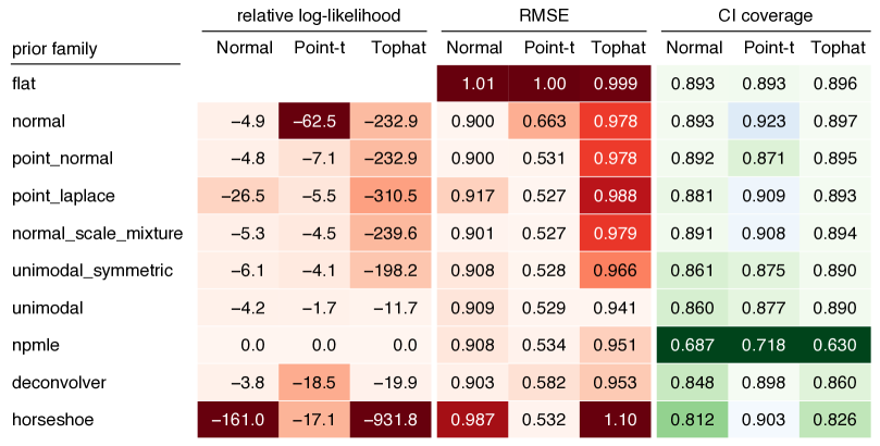
Figure 1: Results of fitting EBNM models with different prior families to “Normal”, “Point-$t$” and “Asymmetric tophat” data sets. For each prior family, the table gives the following quantities averaged across EBNM analyses of 20 data sets with $n=\mbox{1,000}$ observed means: the log-likelihood at $\hat{g}$ relative to the log-likelihood attained by the NPMLE estimate outputted by ebnm() with prior_family = "npmle" (higher log-likelihoods shown with lighter shades of red are better); root mean-squared error (lower RMSEs shown with lighter shades of red are better); and the proportion of credible intervals (90% HPD inverals) containing the true mean (CI coverage values closer to 0.9 shown with lighter shades of green are better).

Figure 1 summarizes results from running EBNM analyses on 10 data sets in each of the three simulation scenarios, with $n=\mbox{1,000}$ observations in each data set. We used the following three measures to evaluate the EBNM model fits:

1. The log-likelihood, which, for ease of interpretation, is shown relative to the log-likelihood attained at the NPMLE estimate. (In theory, the NPMLE estimate should always give the highest likelihood.) These log-likelihoods were obtained by calling logLik() on the ebnm() return value.

2. The root mean-squared error (RMSE), which quantifies how well the estimates recover true means, and is defined as $\mathrm{RMSE}\colonequals\sqrt{\sum_{i=1}^{n}(\hat{\theta}_{i}-\theta_{i})^{2}/n}$, where $\hat{\theta}_{i}$ denotes the posterior mean estimate, $\hat{\theta}_{i}\colonequals\mathbb{E}(\theta_{i}\mid x_{i},s_{i},\hat{g})$. These estimates were obtained by calling coef() on the ebnm() return value.

3. The proportion of true means $\theta_{i}$ that are contained within the credible intervals, which we defined as 90% highest posterior density (HPD) intervals. These credible intervals were obtained by calling confint() on the ebnm() return value.

As expected, the model fit returned by ebnm() with prior_family = "npmle" always attained the largest log-likelihood. More generally, log-likelihoods are expected to align with the ordering implied by the nesting of prior families (17), and indeed, this was largely the case. (Note that deconvolveR sometimes produces log-likelihoods that are worse than less flexible parametric models because it does not directly optimize the log-likelihood, but instead optimizes a penalized log-likelihood.) Prior families that were a poor match with the distribution used to simulate the data typically had worse log-likelihoods. For example, the point-Laplace and horseshoe families had difficulty matching the shape of the normal distribution. In the Asymetric Tophat simulation scenario, all symmetric priors performed poorly by the log-likelihood measure.

The RMSE evaluates the quality of the posterior estimates $\hat{\theta}_{i}$ generated by an EBNM analysis (a lower RMSE is better). As a baseline measure, we computed posterior estimates from the EBNM model with a “flat” prior, which effectively gives us maximum-likelihood estimates $\hat{\theta}_{i}=x_{i}$. Reassuringly, nearly all prior families improved upon the maximum-likelihood estimates, although the improvement was sometimes small, particularly when the prior family was a poor match with the true distribution (e.g., symmetric prior families in the Asymmetric Tophat scenario). The horseshoe family is best suited for “sparse” settings — in which many or most $\theta_{i}$ are zero — and so it was not unexpected that it performed poorly in the Normal and Asymmetric Tophat settings. On the contrary, deconvolveR is best suited for non-sparse settings, which explains its poor performance on the Point-$t$ data sets. Overall, higher log-likelihoods were indicative of better accuracy in estimates of $\theta_{i}$, except when the model overfitted; so for example the NPMLE tended to achieve a better log-likelihood than the unimodal prior in the Asymmetric Tophat scenario, but its accuracy (RMSE) was worse, presumably because of the greater tendency of the NPMLE to overfit.

The “CI coverage” measures how well the credible intervals are calibrated. A known limitation of empirical Bayes methods is that they often underestimate uncertainty in the posteriors (since uncertainty in the estimate of $g$ is not taken into account). Indeed, the HPD intervals tended to be too small (i.e., less than 90%) for most prior families and simulation scenarios (Figure 1). Still, in most cases the intervals were not far off the target coverage of 90%, showing that the CI intervals are surprisingly robust to modeling assumptions. The lone exception was the NPMLE, which tended to have much poorer coverage because, as noted above, it results in a discrete prior that can greatly underestimate uncertainty.

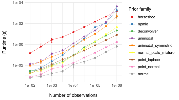
Figure 2: Runtimes for fitting EBNM models with different prior families to data sets ranging in size from $n=100$ to $n=\mbox{1,000,000}$. For each combination of sample size ($n$) and prior family, an EBNM model was fit to 20 data sets simulated using the Point-$t$ distribution. Each point in the plot gives the average runtime over all 20 simulations; the error bars depict 10% and 90% quantiles.

Finally, to assess the ability of our implementation to handle large data sets, we recorded runtimes for simulated (Point-$t$) data sets ranging in size from $n=200$ to $n=\mbox{1,000,000}$. These analyses were performed in R 4.2.2 on a desktop running Windows 11 Pro with an Intel Core i9-13900KF multicore processor and 32 GB of memory. Results are summarized in Figure 2. As expected, the less flexible priors with the fewest parameters tended to also be the fastest, whereas the most complex methods (e.g., unimodal prior, NPMLE) were slower than the fastest methods by several orders of magnitude. Most importantly, all prior families implemented in ebnm scaled well to large data sets; the computational effort grew linearly or close to linearly in $n$.

5 Analyzing weighted on-base averages of MLB players

A longstanding tradition in empirical Bayes research is to include an analysis of batting averages using data from Major League Baseball (see, for example, BrownBaseball; JiangZhangBaseball; GuKoenkerBaseball). Until recently, batting averages were the most important measurement of a hitter’s performance, with the prestigious yearly “batting title” going to the hitter with the highest average. However, with the rise of baseball analytics, metrics that better correlate to teams’ overall run production have become increasingly preferred. One such metric is wOBA (“weighted on-base average”), which is both an excellent measure of a hitter’s offensive production and, unlike competing metrics such as MLB’s xwOBA (xwoba) or Baseball Prospectus’s DRC+ (drcplus), can be calculated using publicly available data and methods.

Initially proposed by Tango, wOBA assigns values (“weights”) to hitting outcomes according to how much the outcome contributes on average to run production. For example, while batting average treats singles identically to home runs, wOBA gives a hitter more than twice as much credit for a home run.

Given a vector of wOBA weights $\mathbf{w}$, hitter $i$’s wOBA is the weighted average

$$x_{i}\colonequals\mathbf{w}^{T}\mathbf{z}^{(i)}/n_{i},$$ (22)

where $\mathbf{z}^{(i)}=(z_{1}^{(i)},\ldots,z_{7}^{(i)})$ tallies outcomes (singles, doubles, triples, home runs, walks, hit-by-pitches, and outs) over the hitter’s $n_{i}$ plate appearances (PAs). Modeling hitting outcomes as i.i.d.

$$\mathbf{z}^{(i)}\sim\text{Multinomial}(n_{i},{\bm{\pi}}^{(i)}),$$ (23)

where ${\bm{\pi}}^{(i)}=(\pi_{1},\ldots,\pi_{7}^{(i)})$ is the vector of “true” outcome probabilities for hitter $i$, we can regard $x_{i}$ as a point estimate for the hitter’s “true wOBA skill”

$$\theta_{i}\colonequals\mathbf{w}^{T}{\bm{\pi}}^{(i)}.$$ (24)

Standard errors for the $x_{i}$’s can be estimated as

$$s_{i}^{2}=\mathbf{w}^{T}\hat{\bm{\Sigma}}^{(i)}\mathbf{w}/n_{i},$$ (25)

where $\hat{\bm{\Sigma}}^{(i)}$ is the estimate of the covariance matrix for the multinomial model (23) obtained by setting ${\bm{\pi}}=\hat{\bm{\pi}}$, where

$$\hat{\bm{\pi}}^{(i)}=\mathbf{z}^{(i)}/n_{i}.$$ (26)

The relative complexity of wOBA makes it well suited for analysis via ebnm. With batting average, a common approach is to obtain empirical Bayes estimates using a beta-binomial model (see, for example, robinson). With wOBA, one can estimate hitting outcome probabilities by way of a Dirichlet-multinomial model; alternatively, one can approximate the likelihood as normal and fit an EBNM model directly to the observed wOBAs. In the following, we take the latter approach.

We begin by loading and inspecting the wOBA data set, which consists of wOBAs and standard errors for the 2022 MLB regular season: R> library(ebnm) R> data(wOBA) R> nrow(wOBA) [1] 688 R> head(wOBA) FanGraphsID Name Team PA x s 1 19952 Khalil Lee NYM 2 1.036 0.733 2 16953 Chadwick Tromp ATL 4 0.852 0.258 3 19608 Otto Lopez TOR 10 0.599 0.162 4 24770 James Outman LAD 16 0.584 0.151 5 8090 Matt Carpenter NYY 154 0.472 0.054 6 15640 Aaron Judge NYY 696 0.458 0.024

Column “x” contains each player’s wOBA for the 2022 season, which we regard as an estimate of the player’s “true” wOBA skill. Column “s” provides standard errors.

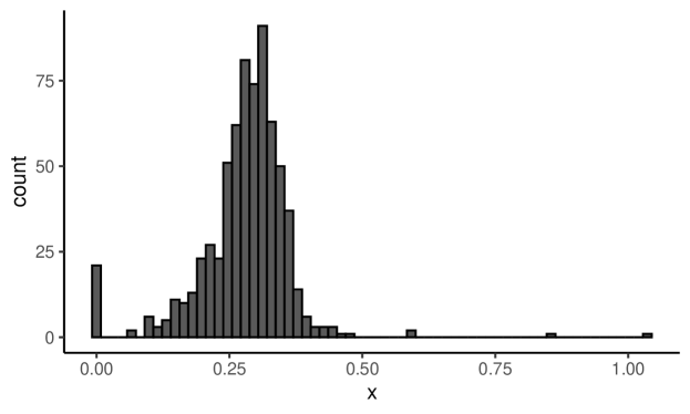
Figure 3: Histogram of MLB player wOBAs from the 2022 season.

Next, we visualize the overall distribution of wOBAs: R> library(ggplot2) R> ggplot(wOBA, aes(x = x)) + + geom_histogram(bins = 64, color = "black") + + theme_classic()

As the histogram (Figure 3) shows, most players finished the season with a wOBA between .200 and .400. A few had very high wOBAs ($>$.500), while others had wOBAs at or near zero. A casual inspection of the data suggests that players with these very high (or very low) wOBAs were simply lucky (or unlucky). For example, the 4 players with the highest wOBAs each had fewer than 16 PAs. It is very unlikely that they would have sustained this high level of production over a full season’s worth of PAs.

In contrast, Aaron Judge’s production — which included a record-breaking number of home runs — appears to be “real,” since it was sustained over nearly 700 PAs. Other cases are more ambiguous: how, for example, are we to assess Matt Carpenter, who had several exceptional seasons between 2013 and 2018 but whose output steeply declined in 2019–2021 before his surprising “comeback” in 2022? An empirical Bayes analysis can help to answer this and other questions.

Function ebnm() is the main interface for fitting the empirical Bayes normal means model (1)–(2); it is a “Swiss army knife” that allows for various choices of prior family $\mathcal{G}$ as well as providing multiple options for fitting and tuning models. For example, we can fit a normal means model with the prior family $\mathcal{G}$ taken to be the family of normal distributions as follows: R> x <- wOBA$xR>s<-wOBA$s R> names(x) <- wOBA$NameR>names(s)<-wOBA$Name R> fit_normal <- ebnm(x, s, prior_family = "normal", mode = "estimate")

(The default behavior is to fix the prior mode at zero. Since we certainly do not expect the distribution of true wOBA skill to have a mode at zero, we set mode = "estimate".)

We note in passing that the ebnm package has a second model-fitting interface, in which each prior family gets its own function: R> fit_normal <- ebnm_normal(x, s, mode = "estimate")

Textual and graphical overviews of results can be obtained using, respectively, methods summary() and plot(). The summary method appears as follows:

R> summary(fit_normal) Call: ebnm_normal(x = x, s = s, mode = "estimate")

EBNM model was fitted to 688 observations with _heteroskedastic_standard errors.

The fitted prior belongs to the _normal_prior family.

2 degrees of freedom were used to estimate the model. The log likelihood is 989.64.

Available posterior summaries: _mean_, _sd_. Use method fitted() to access available summaries.

A posterior sampler is _not_available. One can be added via function ebnm_add_sampler().

The plot() method visualizes results, comparing the “observed” values $x_{i}$ (the initial wOBA estimates) against the empirical Bayes posterior mean estimates $\hat{\theta}_{i}$: R> plot(fit_normal)

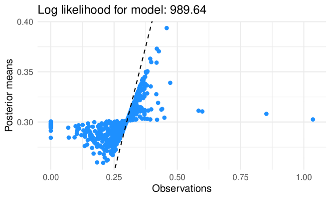
Figure 4: Initial wOBA estimates (“observations”) vs. posterior mean wOBA estimates, in which the posterior estimates were obtained by fitting a prior from the family of normal distributions. The dashed line shows the diagonal $x=y$.

See Figure 4 for this plot. Shrinkage effects are clearly visible, with the most extreme wOBAs on either end of the spectrum being strongly shrunk toward the league average (around .300).

Since plot() returns a “ggplot” object (ggplot2), the plot can conveniently be customized using ggplot2 syntax. For example, one can vary the color of the points by the number of plate appearances: R> plot(fit_normal) + + geom_point(aes(color = sqrt(wOBA$PA)))++labs(x="wOBA",y="EBestimateoftruewOBAskill",color=expression(sqrt(PA)))++scale_{c}olor_{g}radient(low="blue",high="red")SeeFigure\ref{fig:wOBA_normal_custom}forthiscustomizedplot.Byvaryingthecolorofpoints,weseethatthewOBAestimateswithhigherstandarderrorsorfewerplateappearances(bluepoints)tendtobeshrunktowardtheleagueaveragemuchmorestronglythanwOBAsfromhitterswithmanyplateappearances(redpoints).\par\begin{figure}[!t]\centering\includegraphics[width=346.89731pt]{figures/wOBA_normal_custom.pdf}\@@toccaption{{\lx@tag[ ]{{5}}{ThesameasFigure~{}\ref{fig:wOBA_normal},exceptthatthecolorofthepointsisvariedbythenumberofplateappearances.Thedashedlineshowsthediagonal($x=y$)line.}}}\@@caption{{\lx@tag[: ]{{\small Figure 5}}{\small ThesameasFigure~{}\ref{fig:wOBA_normal},exceptthatthecolorofthepointsisvariedbythenumberofplateappearances.Thedashedlineshowsthediagonal($x=y$)line.}}}\@add@centering\end{figure}\par Above,weused\code{head()}toviewdataforthefirst6hittersinthedataset.Let^{\prime}snowseewhattheEBNManalysissuggestsmightbetheir``true^{\prime\prime}wOBAskill.Weusethe\code{fitted()}method,whichreturnsaposteriorsummaryforeachhitter:\CodeChunk\CodeInput>print(head(fitted(fit_{n}ormal)),digits=3)\CodeOutput meansdKhalilLee0.3030.0287ChadwickTromp0.3080.0286OttoLopez0.3100.0283JamesOutman0.3110.0282MattCarpenter0.3390.0254AaronJudge0.3940.0184ThewOBAestimatesofthefirstfourballplayersareshrunkstronglytowardtheleagueaverage,reflectingthefactthattheseplayershadveryfewplateappearances(andindeed,wewerenotswayedbytheirveryhighinitialwOBAestimates).\par Carpenterhadmanymoreplateappearances(154)thantheseotherfourplayers,butaccordingtothismodelweshouldremainskepticalabouthisstrongperformance;afterfactoringintheprior,wejudgehis``true^{\prime\prime}performancetobemuchclosertotheleagueaverage,downgradinganinitialestimateof.472tothefinalposteriormeanestimateof.339.\par\begin{figure}[!t]\centering\includegraphics[width=346.89731pt]{figures/wOBA_comp.pdf}\@@toccaption{{\lx@tag[ ]{{6}}{InitialwOBAestimates(``Observations^{\prime\prime})vs.posteriormeanwOBAestimates,inwhichtheposteriorestimateswereobtainedbyfittingapriorfromthefamilyofnormaldistributions(\code{prior\_family="normal"})andthefamilyofunimodaldistribtions(\code{prior\_family="unimodal"}).Resultsareshownonlyforthetop50ballplayersbynumberofplateappearances.}}}\@@caption{{\lx@tag[: ]{{\small Figure 6}}{\small InitialwOBAestimates(``Observations^{\prime\prime})vs.posteriormeanwOBAestimates,inwhichtheposteriorestimateswereobtainedbyfittingapriorfromthefamilyofnormaldistributions(\code{prior\_family="normal"})andthefamilyofunimodaldistribtions(\code{prior\_family="unimodal"}).Resultsareshownonlyforthetop50ballplayersbynumberofplateappearances.}}}\@add@centering\end{figure}\par Judge^{\prime}s``true^{\prime\prime}wOBAisalsoestimatedtobemuchlower(.394)thantheinitialestimate(.458)despitesustainingthishighlevelofproductionoverafullseason(696PAs).Forthisreason,onemightaskwhetherapriorthatismoreflexiblethanthenormalprior---thatis,apriorthatcanbetteradaptto``outliers^{\prime\prime}likeJudge---mightproduceadifferentresult.The\pkg{ebnm}packageisverywellsuitedtoansweringthisquestion.Forexample,toobtainresultsusinga``unimodal^{\prime\prime}priorinsteadofanormalprior,weneedonlychange\code{prior_{f}amily}from\code{"normal"}to\code{"unimodal"}:\CodeChunk\CodeInput R>fit_{u}nimodal<-ebnm(x,s,prior_{f}amily="unimodal",mode="estimate")Itisstraightforwardtoproduceaside-by-sidevisualizationofthefittedmodelssimplybyincludingbothmodelsasargumentstothe\code{plot()}method:\CodeChunk\CodeInput top50<-order(wOBA$PA,decreasing=TRUE)top50<-top50[1:50]plot(fit_{n}ormal,fit_{u}nimodal,subset=top50)Wealsousedthe\code{subset}argumenttofocusontheresultsforJudgeandotherplayerswiththemostplateappearances.TheplotresultingfromthiscallisshowninFigure\ref{fig:wOBA_comp}.Indeed,thisplotillustratestheabilityoftheunimodalpriortobetteradapttothedata:wOBAestimatesforplayerswithalotofplateappearancesarenotadjustedquitesostronglytowardtheleagueaverage.Tocompareinmoredetail,weseeforexamplethatJudge^{\prime}swOBAestimatefromthemodelwiththeunimodalprior(the\code{"mean2"}column)remainsmuchclosertotheoriginalwOBAestimate:\CodeChunk\CodeInput R>dat<-cbind(wOBA[,c("PA","x")],+fitted(fit_{n}ormal),+fitted(fit_{u}nimodal))R>names(dat)<-c("PA","x","mean1","sd1","mean2","sd2")R>print(head(dat),digits=3)\CodeOutput PAxmean1sd1mean2sd2KhalilLee21.0360.3030.02870.3020.0277ChadwickTromp40.8520.3080.02860.3070.0306OttoLopez100.5990.3100.02830.3100.0315JamesOutman160.5840.3110.02820.3110.0318MattCarpenter1540.4720.3390.02540.3550.0430AaronJudge6960.4580.3940.01840.4390.0155Carpenter^{\prime}swOBAestimateisalsohigherunderthemoreflexibleunimodalprior,butisstilladjustedmuchmorethanJudge^{\prime}sinlightofCarpenter^{\prime}ssmallersamplesize.Itisalsointerestingthattheunimodalpriorassignsgreateruncertainty(the\code{"sd2"}column)tothisestimatecomparedtothenormalprior.\par\begin{figure}[!t]\centering\includegraphics[width=433.62pt]{figures/wOBA_comp_cdf.pdf}\@@toccaption{{\lx@tag[ ]{{7}}{Thecumulativedistributionfunctions(CDFs)forthepriorsthatwerefittedtothe2022MLBwOBAdata:thenormalprior(\code{prior\_family="normal"})andtheunimodalprior(\code{prior\_family="unimodal"}).Theright-handpanelshowstherighttailofthepriorsinmoredetail.}}}\@@caption{{\lx@tag[: ]{{\small Figure 7}}{\small Thecumulativedistributionfunctions(CDFs)forthepriorsthatwerefittedtothe2022MLBwOBAdata:thenormalprior(\code{prior\_family="normal"})andtheunimodalprior(\code{prior\_family="unimodal"}).Theright-handpanelshowstherighttailofthepriorsinmoredetail.}}}\@add@centering\end{figure}\par\par Recallthatthetwonormalmeansmodelsdifferonlyinthepriorsused,sowecanunderstandthedifferencesintheshrinkagebehaviorofthesemodelsbyinspectingthepriors.Calling\code{plot()}with\code{incl_{c}df=TRUE}showsthecumulativedistributionfunctions(CDFs)ofthefittedpriors$^g$.SinceweareparticularlyinterestedinunderstandingthedifferencesinshrinkagebehaviourforthelargestwOBAssuchasJudge^{\prime}s,wecreateasecondplotthatzoomsinonwOBAsover.350:\CodeChunk\CodeInput R>plot(fit_{n}ormal,fit_{u}nimodal,incl_{c}df=TRUE,incl_{p}m=FALSE)++xlim(c(0.250,0.450))++guides(color="none")R>plot(fit_{n}ormal,fit_{u}nimodal,incl_{c}df=TRUE,incl_{p}m=FALSE)++xlim(c(0.350,0.450))++ylim(c(0.95,1))TheseplotsareshowninFigure\ref{fig:wOBA_comp_cdf}.TheplotontherightshowsthatthefittednormalpriorhasalmostnomassonwOBAsabove.400,explainingwhyJudge^{\prime}swOBAestimateisshrunksostronglytowardtheleagueaverage,whereastheunimodalpriorisflexibleenoughtopermitlargerposteriorestimatesabove.400.\par\par Theposteriormeansandstandarderrorsreturnedfromthe\code{ebnm()}callcannotbeusedtoobtaincredibleintervals(exceptforthespecialcaseofthenormalprior).Therefore,weprovideadditionalmethods\code{confint()}and\code{quantile()}whichreturn,respectively,credibleintervals(ormoreprecisely,{\em highestposteriordensity}intervals:{\cite[citet]{\@@bibref{Authors Phrase1YearPhrase2}{hpd, chen-1999}{\@@citephrase{}}{\@@citephrase{}}}})andposteriorquantilesforeachobservation.TheseareimplementedusingMonteCarlotechniques,whichcanbeslowforlargedatasets,socredibleintervalsarenotcomputedbydefault.Thefollowingcodecomputes80\%highestposteriordensity(HPD)intervalsfortheEBNMmodelwithunimodalprior.(WeaddaMonteCarlosamplerusingfunction\code{ebnm_{a}dd_{s}ampler()};alternatively,wecouldhaveaddedasamplerinourinitialcallsto\code{ebnm()}byspecifying\code{output=output_{a}ll()}.)Wesetaseedforreproducibility:\CodeChunk\CodeInput R>fit_{u}nimodal<-ebnm_{a}dd_{s}ampler(fit_{u}nimodal)R>set.seed(1)R>print(head(confint(fit_{u}nimodal,level=0.8)),digits=3)\CodeOutput CI.lowerCI.upperKhalilLee0.2770.328ChadwickTromp0.2770.334OttoLopez0.2770.336JamesOutman0.2770.335MattCarpenter0.2770.389AaronJudge0.4280.458Interestingly,the80\%credibleintervalforCarpenterisverywide,andsharesthesamelowerboundasthefirstfourballplayerswithveryfewplateappearances.\par\par\par$

5.1 Reanalyzing the baseball data using a nonparametric prior

Above, we demonstrated how the ebnm package makes it is easy to perform EBNM analyses with different types of priors, then compare results across different prior choices. Each prior family makes different assumptions about the data which, a priori, may be more or less plausible. An alternative to prior families that make specific assumptions about the data is to use the prior family that contains all distributions $\mathcal{G}_{\mathrm{npmle}}$, which is in a sense “assumption free” (see Section 2 for background). Here we re-analyze the wOBA data set to illustrate the use of this prior family. Note that although nonparametric priors require specialized computational techniques, switching to a nonparametric prior is seamless in ebnm, as these implementation details are hidden. Similar to above, we need only make a single change to the prior_family argument: R> fit_npmle <- ebnm(x, s, prior_family = "npmle") (Note that because the family $\mathcal{G}_{\mathrm{npmle}}$ is not unimodal, the mode = "estimate" option is not relevant here.)

Although the implementation details are hidden by default, it can sometimes be helpful to see what is going on “behind the scenes,” particularly for flagging or diagnosing issues. By default, ebnm uses the mixsqp package (MixSQP) to fit the NPMLE $\hat{g}\in\mathcal{G}_{\mathrm{npmle}}$. We can monitor convergence of the mix-SQP optimization algorithm by setting the verbose control argument to TRUE: R> fit_npmle <- ebnm(x, s, prior_family = "npmle", + control = list(verbose = TRUE)) Running mix-SQP algorithm 0.3-48 on 688 x 95 matrix convergence tol. (SQP): 1.0e-08 conv. tol. (active-set): 1.0e-10 zero threshold (solution): 1.0e-08 zero thresh. (search dir.): 1.0e-14 l.s. sufficient decrease: 1.0e-02 step size reduction factor: 7.5e-01 minimum step size: 1.0e-08 max. iter (SQP): 1000 max. iter (active-set): 20 number of EM iterations: 10 Computing SVD of 688 x 95 matrix. Matrix is not low-rank; falling back to full matrix. iter objective max(rdual) nnz stepsize max.diff nqp nls 1 +9.583407733e-01 – EM – 95 1.00e+00 6.08e-02 – – 2 +8.298700300e-01 – EM – 95 1.00e+00 2.87e-02 – – 3 +7.955308369e-01 – EM – 95 1.00e+00 1.60e-02 – – 4 +7.819858634e-01 – EM – 68 1.00e+00 1.05e-02 – – 5 +7.753787534e-01 – EM – 53 1.00e+00 7.57e-03 – – 6 +7.717040208e-01 – EM – 49 1.00e+00 5.73e-03 – – 7 +7.694760705e-01 – EM – 47 1.00e+00 4.48e-03 – – 8 +7.680398878e-01 – EM – 47 1.00e+00 3.58e-03 – – 9 +7.670690681e-01 – EM – 44 1.00e+00 2.91e-03 – – 10 +7.663865515e-01 – EM – 42 1.00e+00 2.40e-03 – – 1 +7.658902386e-01 +6.493e-02 39 —— —— – – 2 +7.655114904e-01 +5.285e-02 19 1.00e+00 9.88e-02 20 1 3 +7.627839841e-01 +1.411e-02 7 1.00e+00 1.28e-01 20 1 4 +7.626270875e-01 +2.494e-04 7 1.00e+00 3.23e-01 8 1 5 +7.626270755e-01 +1.748e-08 7 1.00e+00 4.94e-04 2 1 6 +7.626270755e-01 -2.796e-08 7 1.00e+00 2.76e-07 2 1 Optimization took 0.03 seconds. Convergence criteria met—optimal solution found. This output shows no issues with convergence of the optimization algorithm; the mix-SQP algorithm converged to the solution (up to numerical rounding error) in only 6 iterations. In some cases, convergence issues can arise when fitting nonparametric models to large or complex data sets, and revealing the details of the optimization can help to pinpoint these issues.

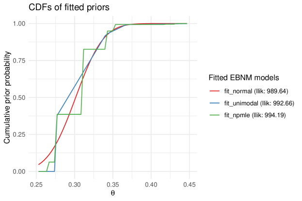
Figure 8: The CDFs for priors fitted to the 2022 MLB wOBA data: the normal prior (prior_family = "normal"), the unimodal prior (prior_family = "unimodal"), and the NPMLE (prior_family = "npmle").

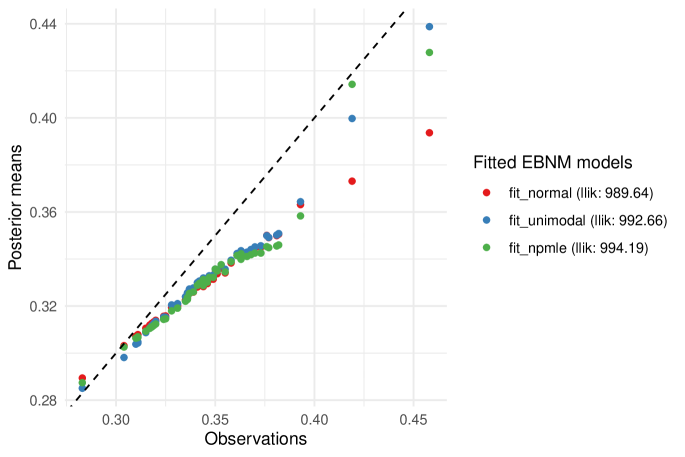
Figure 9: Initial wOBA estimates (“Observations”) vs. posterior mean wOBA estimates for priors fitted to the 2022 MLB wOBA data: the normal prior (prior_family = "normal"), the unimodal prior (prior_family = "unimodal"), and the NPMLE (prior_family = "npmle"). Results are shown only for the top 50 ballplayers by number of plate appearances.

Next, we visually compare the three fits obtained so far: plot(fit_normal, fit_unimodal, fit_npmle, incl_cdf = TRUE, subset = top50) The plots generated by this call are shown in Figures 8 and 9. As before, estimates largely agree, differing primarily at the tails. Both the unimodal prior family and the NPMLE are sufficiently flexible to avoid the strong shrinkage behavior of the normal prior family.

Fits can be compared quantitatively using the logLik() method, which, in addition to the log likelihood for each model, usefully reports the number of free parameters (i.e., degrees of freedom): R> logLik(fit_unimodal) ’log Lik.’ 992.6578 (df=40) R> logLik(fit_npmle) ’log Lik.’ 994.193 (df=94) A nonparametric prior $\mathcal{G}$ is approximated by $K$ mixture components on a fixed grid, with the mixture proportions to be estimated (see Section 2). We can infer from the above output that $\mathcal{G}_{\text{npmle}}$ has been approximated as a family of mixtures over a grid of $K=95$ point masses spanning the range of the data. (The number of degrees of freedom is one fewer than $K$ because the mixture proportions must always sum to 1, which removes one degree of freedom from the estimation of ${\bm{\pi}}$.)

The default behaviour for nonparametric prior families is to choose $K$ such that the likelihood obtained using estimate $\hat{g}$ should be (on average) within one log-likelihood unit of the optimal estimate from among the entire nonparametric family $\mathcal{G}$ (that is, provided that the “true” prior is $g\in\mathcal{G}$; see WillwerscheidDiss). Thus, a finer approximating grid should not yield a large improvement in the log-likelihood. We can check this by using ebnm_scale_npmle() to create a finer grid: R> scale_npmle <- ebnm_scale_npmle(x, s, KLdiv_target = 0.001/length(x), + max_K = 1000) R> fit_npmle_finer <- ebnm_npmle(x, s, scale = scale_npmle) R> logLik(fit_npmle) ’log Lik.’ 994.193 (df=94) R> logLik(fit_npmle_finer) ’log Lik.’ 994.2502 (df=528) As the theory predicts, a much finer grid, with $K=529$, results in only a modest improvement in the log-likelihood. ebnm provides similar functions to customize grids for unimodal and normal scale mixture prior families.

One potential issue with the NPMLE is that, since it is discrete (as the CDF plot in Figure 8 makes apparent), observations are variously shrunk toward one of the support points, which can result in poor interval estimates. For illustration, we calculate 10% and 90% quantiles: R> fit_npmle <- ebnm_add