Liu, Fang and Lu

Lagrangian Inference for Ranking Problems

Lagrangian Inference for Ranking Problems

Yue Liu Department of Statistics, Harvard University, Boston, MA 02138, yueliu@fas.harvard.eduEthan X. Fang Department of Statistics, Pennsylvania State University, University Park, PA 16802, xxf13@psu.edu Junwei Lu Department of Biostatistics, Harvard T.H. Chan School of Public Health, Boston, MA 02130, junweilu@hsph.harvard.edu

We propose a novel combinatorial inference framework to conduct general uncertainty quantification in ranking problems. We consider the widely adopted Bradley-Terry-Luce (BTL) model, where each item is assigned a positive preference score that determines the Bernoulli distributions of pairwise comparisons’ outcomes. Our proposed method aims to infer general ranking properties of the BTL model. The general ranking properties include the “local” properties such as if an item is preferred over another and the “global” properties such as if an item is among the top $K$-ranked items. We further generalize our inferential framework to multiple testing problems where we control the false discovery rate (FDR), and apply the method to infer the top-$K$ ranked items. We also derive the information-theoretic lower bound to justify the minimax optimality of the proposed method. We conduct extensive numerical studies using both synthetic and real datasets to back up our theory.

Combinatorial inference, Ranking, Pairwise comparisons, Bradley-Terry-Luce model, Minimax lower bound.

1 Introduction

Ranking problems aim to study relative orderings of some set of items, and find many applications such as sports competition (Massey 1997, Pelechrinis et al. 2016, Price 2017, Xia et al. 2018), online gamers ranking (e.g., Microsoft TrueSkill ranking system Minka et al. (2007, 2018)), web search and information retrieval (Dwork et al. 2001, Bouadjenek et al. 2013, Guo et al. 2020), recommendation systems (Baltrunas et al. 2010, He et al. 2018, Geyik et al. 2019), crowdsourcing (Chen et al. 2013, Suh et al. 2017, Liang and de Alfaro 2020), gene ranking (Boulesteix and Slawski 2009, Kolde et al. 2012, Kim et al. 2015), assortment optimization (Li et al. 2018, Aouad et al. 2018), among many others. Due to the practical importance, ranking problems draw significant attention from different communities such as operations research (McFadden 1973, Mohammadi and Rezaei 2020), statistics (Hunter 2004, Chen et al. 2020), machine learning (Richardson et al. 2006, Guo et al. 2020), and sociology (Brown 2003, Subochev et al. 2018).

In ranking problems, given some comparisons among pairs of $n$ items, we aim to infer the relative ranking of these items. Many models are proposed to study this problem, and one of the most widely used parametric models is the Bradley-Terry-Luce (BTL) model (Bradley and Terry 1952, Luce 1959). In the BTL model, each item is assigned a latent positive preference score that determines its rank, and the latent scores determine the relative preference among the $n$ items.

Based on the BTL model, there are several tracks of works that estimate the ranks of the items by estimating the latent scores. The first track is the rank centrality method (Negahban et al. 2017, Dwork et al. 2001, Maystre and Grossglauser 2015, Vigna 2016, Jang et al. 2016), which is also known as the spectral method. This class of methods connects pairwise comparisons with random walk over the comparison graph. In particular, each node in the graph represents an item, and the probability of moving from node $i$ to node $j$ equals the probability that item $j$ is preferred over item $i$. Based on this approach, Negahban et al. (2017) show that the preference scores of items coincide the stationary distribution under the random walk, and derive a fast rate of convergence of the estimator for the scores. Chen et al. (2019) further improve the convergence rate in Negahban et al. (2017) by removing the logarithmic factor. The second track is based on considering the regularized maximum likelihood estimator (MLE) (Ford Jr 1957, Hunter 2004, Lu and Negahban 2015). This approach estimates the latent scores by maximizing the regularized likelihood function, and Chen et al. (2019) derive the rate of convergence of the estimator under the $\ell_{2}$ regularization. Negahban et al. (2018) also consider nuclear norm regularization. In addition, Azari Soufiani et al. (2013) consider the method of moments for the Plackett-Luce model, and Mosteller (2006), Jiang et al. (2011), Neudorfer and Rosset (2018) consider general least square methods, and their estimation consistency for preference scores are established by various works (Chen and Suh 2015, Maystre and Grossglauser 2015, Jang et al. 2016, Duchi et al. 2010, Rajkumar and Agarwal 2014, 2016).

Despite the aforementioned significant progress of rank estimation, the uncertainty quantification in ranking problems remains largely unexplored, which is of crucial importance in practice. For example, saying that player $i$ is ranked higher than player $j$ without a confidence score is not very informative in practice. In this paper, we propose a novel combinatorial inferential framework for testing ranking properties. In particular, given $n$ items, we define a ranking list $\gamma$ as a permutation over the set of $n$ items $[n]=\{1,...,n\}$, and let $\mathcal{R}$ be the set of all possible rankings (i.e., all possible permutation over $[n]$). Let ranking list $\gamma^{*}$ be the true underlying ranking of $n$ items. We aim to test whether $\gamma^{*}$ satisfies certain ranking properties based on partial pairwise comparison observations. For example, let $\mathcal{R}_{i}$ be a subset of $\mathcal{R}$ representing the ranking property with respect to item $i$. We test the general ranking property for a given item $i$, i.e., whether item $i$ has certain properties, i.e.,

$${H}_{0}:\text{item }i\text{ does not satisfy the property}\text{ \ \ v.s. \ \ }{H}_{a}:\text{item }i\text{ satisfies the property},$$

which is equivalent to

$${H}_{0}:\gamma^{*}\notin\mathcal{R}_{i}\text{ \ \ v.s. \ \ }{H}_{a}:\gamma^{*}\in\mathcal{R}_{i}.$$

1.1 Motivating Applications

The inference in ranking problems finds many applications. For instance, it is of practical interest to test whether movie $A$ is preferred over movie $B$ on average, and test whether chess player $C$ is stronger than player $D$. Such problems are pairwise ranking inference problems that fit into our framework as defined in the following example.

Example 1.1 (Pairwise ranking inference)

Consider testing whether item $i$ is ranked higher than item $j$. Let $\mathcal{R}_{i}$ be the set of all possible rankings that item $i$ is ranked higher than item $j$. We consider the following hypothesis testing problem that

$${H}_{0}:\text{Item }j\text{ is ranked higher than item }i\text{ \ \ v.s. \ \ }{H}_{a}:\text{Item }i\text{ is ranked higher than item }j.$$

Another important application of inference in ranking problems is the top-$K$ inference. For instance, in recommendation systems, one important goal is to find a few most appealing items for the users (Cremonesi et al. 2010). In biomedical studies, only a small subset of top-ranked genes is informative, and it is crucial for the investigators to identify this set of genes to perform detailed analysis (Boulesteix and Slawski 2009). In assortment optimization, the challenge is to identify a subset of items that maximize revenue based on customer preferences (Li et al. 2018, Aouad et al. 2018). We first summarize the single top-$K$ inference problem in the following example.

Example 1.2 (Single top-$K$ inference)

Consider testing whether item $i$ is among the top-$K$ items (a special case is $K=1$). Here $\mathcal{R}_{i}$ is the set of all possible rankings that item $i$ is among the top-$K$ items. We consider the following hypothesis testing problem that

$${H}_{0}:\text{Item }i\text{ is not among the top-$K$ items}\text{ \ \ v.s. \ \ }{H}_{a}:\text{Item }i\text{ is among the top-$K$ items}.$$

We then extend the problem to the multiple testing setup, where the goal is to infer the set of all top-$K$ items.

Example 1.3 (Top-$K$ inference)

Consider the problem of identifying the set of top-$K$ items. Here $\mathcal{R}_{i}$ is the set of all possible rankings that item $i$ is among the top-$K$ items, $i\in[n]$. We consider the following multiple testing problem that

$${H}_{0}:\text{Item $i$ is not among the top-$K$ items}\text{ \ v.s. \ }{H}_{a}:\text{Item $i$ is among the top-$K$ items,}\text{ \ for\ }i\in[n].$$

1.2 Major Contributions

To the best of our knowledge, this paper provides the first inferential framework for ranking problems. Our proposed method can test a broad class of hypotheses for ranking problems. Theoretically, we show that the p-values are valid, and our procedures are powerful. We summarize the major contributions below.

• We are among the first to study general inferential approaches for ranking problems beyond estimation, and we propose a novel general framework for inferring different ranking properties. We show that our proposed methods are asymptotically valid and powerful. Furthermore, we generalize the method to the more challenging multiple testing setup to widen the applicability.

• In our inferential framework, we propose a novel general Lagrangian debiasing procedure to handle the constrained parameter space. Our Lagrangian debiasing procedure addresses the challenge raised by the non-identifiability of the BTL model. Most existing works on high-dimensional inference, such as Zhang and Zhang (2014), Van de Geer et al. (2014), Ning and Liu (2017), focus on inferring the parameter under the unconstrained space, and do not apply to the BTL model due to the constraints. By considering the optimality condition of the Lagrangian dual problem, our proposed approach provides a new tool for high-dimensional inference under general constraints. We also derive the asymptotic distribution of our debiased estimator. We point out that this new Lagrangian debiasing procedure can be applied to general high-dimensional constrained inferential problems beyond ranking problems, which itself is of great interest.

• We provide a new framework to derive the minimax lower bound for multiple testing in ranking problems, which provides new theoretical insights. To the best of our knowledge, this is the first time that such a lower bound is derived. In particular, let the preference score vector be $\theta\in\mathbb{R}^{n}$, which represents the scores of all $n$ items that determine the ranks of all items. We first define a new minimax risk for the multiple testing problems that

  $$\mathfrak{R}=\inf_{\psi}\sup_{\theta}{\mathbb{P}}(\char 35\relax\text{ false positives}+\char 35\relax\text{ false negatives}\geq 1),$$

  where the infimum is taken over all possible selection procedure $\psi$. Here the risk is the probability of making at least one Type I or Type II error. If the minimax risk $\mathfrak{R}\geq\ 1-\epsilon$ for some constant $\epsilon>0$, we say that any procedure fails for the multiple testing problem since they cannot control the Type I error or Type II error in the minimax sense. To derive the necessary conditions for controlling minimax risk, we further define a novel distance $\Delta({\theta})$ in (18), and a divider set $\mathcal{M}({\theta})$ in Definition 5.1, which capture the combinatorial structures of ranking properties. Intuitively, the distance is a signal strength for selecting the items of interest; the divider set is the set of items that are crucial for selecting the items, and the size of the divider set increases as the distance decreases. We show that the numerical signal strength $\Delta({\theta})$ and combinatorial signal strength $|\mathcal{M}({\theta})|$ together measure the difficulty in the multiple testing problems. We also give two concrete examples where $\mathfrak{R}$ is arbitrarily close to 1 if $\Delta({\theta})\lesssim\sqrt{\frac{\log n}{npL}}$. In addition, we show that our lower bound matches our upper bound to justify the optimality of the proposed method.

1.3 Literature Review

Ranking Problem. There has been a long history of works on ranking problems (Mallows 1957, Keener 1993, Altman and Tennenholtz 2005, Jiang et al. 2011, Osting et al. 2013, Vigna 2016, Ding et al. 2018, Filiberto et al. 2018, Guo et al. 2020, Pujahari and Sisodia 2020). Some ranking systems are based on explicit preference scores or ratings provided by individuals, which is closely related to the matrix completion problem (Candès and Recht 2009, Negahban and Wainwright 2012). In these problems, an individual only provides scores for a subset of items, and we estimate the individual’s preference scores for other items. However, users’ explicit scores can be inconsistent and noisy, or even not available in some cases. This motivates researchers to develop methods for ranking aggregations from comparison results or partial rankings provided by users (Saaty 2003, Ailon et al. 2008, Ailon 2010, Gleich and Lim 2011, Ammar and Shah 2011, Farnoud et al. 2012, Volkovs and Zemel 2012, Ammar and Shah 2012, Swain et al. 2017, Nápoles et al. 2017, Jang et al. 2017, 2018, Chen et al. 2018b, Zhang 2020).

Another important track of works on ranking problems are based on pairwise comparison data (Kendall and Smith 1940, Kendall 1955, Adler et al. 1994, Talluri and Van Ryzin 2006, Chen et al. 2017, Beutel et al. 2019, Jain et al. 2020, Chen et al. 2021). For instance, Lu and Boutilier (2011) study the Mallows model from pairwise comparisons. Chen et al. (2017) study the sequential design with pairwise comparisons. Chen and Suh (2015) propose a new two-step method called the spectral MLE, and prove that it is minimax optimal. Jang et al. (2016) show that the spectral method itself is optimal for identifying the top-$K$ items in the sense of achieving the minimal sample size. Chen et al. (2019) further study the sample complexity of regularized MLE and spectral method in a sparse pairwise comparison setting.

There are other general frameworks on ranking problems such as the Thurstone model (Thurstone 1927, Vojnovic and Yun 2017, Orbán-Mihálykó et al. 2019, Jin et al. 2020) and Plackett-Luce model (Guiver and Snelson 2009, Hajek et al. 2014). For instance, Jin et al. (2020) propose a heterogeneous Thurstone model capturing heterogeneity of different individuals, and propose an algorithm to estimate the preference score vector and heterogeneity. Beyond parametric models, there are also nonparametric methods for ranking problems. For instance, Shah and Wainwright (2017) analyze a simple counting algorithm proposed by Copeland (1951), which counts the numbers of wins of each item, and show its optimality and robustness. Shah et al. (2016), Chen et al. (2018a), and Pananjady et al. (2017) consider the strong stochastically transitive (SST) model for pairwise comparisons. Furthermore, some other works consider ranking problems under specific settings such as active-ranking (Jamieson and Nowak 2011, Busa-Fekete et al. 2013, Heckel et al. 2019), and crowd-sourcing (Chen et al. 2013, 2016, Suh et al. 2017, Liang and de Alfaro 2020). However, we point out the all above works focus on the estimation problem, and do not consider uncertainty quantification and inferential methods in ranking. One exception is Hall and Miller (2009). This work focuses on using $m$-out-of-$n$ bootstrap to estimate the distribution of an empirical rank, which requires empirical choice of $m$ and is of less practical interest. In contrast, we provide a more general framework that solves the problems of practical interest.

Constrained Inference. The inference under equality or inequality constraints is of great interest in literature. The low-dimensional constrained inference dates back to Chernoff (1954), which proves that the likelihood ratio weakly converges to a weighted chi-square distribution for constrained testings. Under the low-dimensional setting, the constrained inference has been further studied in Gourieroux et al. (1982), Kodde and Palm (1986), Rogers (1986), Shapiro (1988), Wolak (1989), Molenberghs and Verbeke (2007), Susko (2013), among many others. For the high-dimensional constrained inference, Yu et al. (2019) assume the existence of natural constraint on parameters, and test whether the parameters lie on the boundary of the constraint. By applying the debiasing approach in Ning and Liu (2017), the authors study the asymptotic distribution of test statistics under constraints.

We note that the above mentioned methods cannot be applied to solve our problem. This is mainly due to the unique challenge that in our setting, the Fisher information matrix is singular due to the non-identifiability issue.

Paper Organization. The rest of our paper is organized as follows. In Section 2, we introduce some preliminaries of ranking problems and some ranking properties. In Section 3, we present our debiased estimator with constraints. We then provide the general hypothesis testing. In Section 4, we extend our method to handle multiple testing problems. In Section 5, we present the lower bound theory with applications to several examples. We provide numerical results in Section 6 and some discussions in Section 7.

Notations. Let $|A|$ represent the cardinality of set $A$, and $[n]$ represent the set of $\{1,\cdots,n\}$ for $n\in\mathbb{Z}^{+}$. For vector $v=\left(v_{1},\ldots,v_{d}\right)^{T}\in\mathbb{R}^{d}$, and $1\leq q\leq\infty,$ we define norm of $v$ as $\|v\|_{q}=\big{(}\sum_{i=1}^{d}\left|v_{i}\right|^{q}\big{)}^{1/q}$. In particular, $\|v\|_{\infty}=\max_{1\leq i\leq d}\left|v_{i}\right|$. For a matrix $M=\left[M_{ij}\right]$, let $\ell_{1}$-norm $\|M\|_{1}=\max_{j}\sum_{i}\left|M_{ij}\right|$, $\ell_{\infty}$-norm $\|M\|_{\infty}=\max_{i}\sum_{j}\left|M_{ij}\right|$, and the operator norm $\|M\|_{2}=\sigma_{\max}(M)$ where $\sigma_{\max}(M)$ represents the largest singular value of matrix $M$. In addition, $a_{n}=O(b_{n})$ or $a_{n}\lesssim b_{n}$ means there exists a constant $C>0$ such that $a_{n}\leq Cb_{n}$, and $a_{n}=o(b_{n})$ means $\lim_{n\rightarrow\infty}\frac{a_{n}}{b_{n}}=0$. we write $a_{n}\asymp b_{n}$ if $C\leq a_{n}/b_{n}\leq C^{\prime}$ for some $C,C^{\prime}>0$. For a sequence of random variables $\{X_{n}\}$, we write $X_{n}\overset{d}{\longrightarrow}X$ if $X_{n}$ converges in distribution to the random variable $X$. Throughout the paper, we let $C,C_{1},C_{2},\cdots,c,c_{1},c_{2},\cdots$ be generic constants which may change in different places.

2 Preliminaries and Problem Setup

In this section, we provide some preliminaries to facilitate our discussions. We first briefly review the Bradley-Terry-Luce model and introduce our data generating scheme. Then, we provide the definitions of rankings and ranking properties.

2.1 Bradley-Terry-Luce Model

We consider the Bradley-Terry-Luce (BTL) parametric model (Bradley and Terry 1952, Luce 1959). This model assumes a hidden preference score $\omega^{*}_{i}>0$ for each item $i$, $1\leq i\leq n$. The scores determine the ranking and the distributions of comparison results. Let ${\omega}^{*}=(\omega^{*}_{1},\cdots,\omega^{*}_{n})^{\top}\in\mathbb{R}^{n}$ be the true preference score vector, and its log-transformation is

$${\theta}^{*}=(\theta^{*}_{1},\cdots,\theta^{*}_{n})^{\top},\text{ where }\theta^{*}_{i}=\log\omega^{*}_{i}.$$

Here $\omega^{*}_{j}>\omega^{*}_{i}$ or $\theta^{*}_{j}>\theta^{*}_{i}$ means that item $j$ is ranked higher (preferred) than item $i$. In this paper, for ease of presentation, we consider the case that all scores are in a bounded domain that $w_{i}^{*}\in\left[w_{\min},w_{\max}\right]$ for all $i\in[n]$, where $w_{\min},\ w_{\max}>0$. We let $\kappa=\omega_{\max}/\omega_{\min}$ be the condition number, and $\kappa$ is a constant which does not depend on $n$.

When we collect data, we compare the items pairwisely. To model the random pairs for comparisons, we adopt the Erdös-Rényi random graph. In particular, suppose we have an undirected graph $\mathcal{G}=\{\mathcal{V},\mathcal{E}\}$ where $\mathcal{V}=[n]$ is the vertex set, and $\mathcal{E}\subseteq[n]\times[n]$ is the edge set. In the Erdös-Rényi random graph $\mathcal{G}(n,p)$, each edge is drawn independently from a Bernoulli distribution with probability $p$. Here we assume that for each pair $(i,j)\in\mathcal{E}$, we observe the comparisons $L$ times. Note that we assume for all pairs in $\mathcal{E}$, we have a same number of observations for ease of presentation, but our proposed method can be easily generalized to handle the general setting where we have different numbers of observations of different pairs. Denote by $y_{i,j}^{(\ell)}$ the $\ell$-th comparison between items $i$ and $j$ for some $i<j$, which depends only on the relative scores of the two items. We assume that each $y_{i,j}^{(\ell)}$ is generated independently from a Bernoulli distribution that

$$y_{i,j}^{(\ell)}\stackrel{{\scriptstyle\text{ ind. }}}{{=}}\left\{\begin{array}[]{ll}1,&\text{ with probability }\frac{w_{j}^{*}}{w_{i}^{*}+w_{j}^{*}}=\frac{e^{\theta_{j}^{*}}}{e^{\theta_{i}^{*}}+e^{\theta_{j}^{*}}}\\ 0,&\text{ otherwise,}\end{array}\right.$$ (1)

where $y_{i,j}^{(\ell)}=1$ means item $j$ is preferred over item $i$. Here we assume that all $y_{i,j}^{(\ell)}$’s are independent for all $i,j$, $(i<j)$, and $\ell$.

We point out that the BTL model is invariant that if we multiply $\omega_{i}^{*}$, or increase $\theta^{*}$, by a constant $c$, the distribution of ${y}_{i,j}^{(\ell)}$ does not change. That is, ${\theta}^{*}$ and ${\theta}^{*}+c=(\theta^{*}_{1}+c,\cdots,\theta^{*}_{n}+c)^{\top}$ are observationally equivalent. Hence, we regard a score vector ${\theta}^{*}\in\mathbb{R}^{n}$ as an equivalence class $[{\theta}^{*}]=\{{\theta}^{\prime}:{\theta}^{*}+c,c\in\mathbb{R}\}$, and regard the parameter space as the set of equivalence classes of $\mathbb{R}^{n}$ (Hunter 2004, Negahban et al. 2017). For the identifiability of the parameters, we impose a constraint on the parameter space $\mathcal{C}$ that we let $\mathcal{C}=\{\theta:f(\theta)=0\}$, and propose our inferential framework under this constraint, where the function $f$ is smooth, and ensures the identifiability of the parameter $\theta$. Specific examples of $f$ include $\bm{1}^{\top}{\theta}=0$, ${\theta}_{1}=1$ (${\theta}_{1}$ is the preference score of the first item), among others (Negahban et al. 2017, Jin et al. 2020, Chen et al. 2013).

2.2 Ranking and Ranking Property

As discussed in the introduction, our goal is to infer some general ranking properties based on the BTL model using samples of pairwise comparisons among all items. We first provide the formal definition of the ranking and its properties.

Definition 2.1 (Ranking)

Assume there are $n$ items. Let $\mathcal{R}$ be all bijections from the set $[n]$ onto itself. Then each $\gamma\in\mathcal{R}$ is a possible rank of the $n$ items. Let $\gamma_{i}$ be the rank of item $i$ in ranking $\gamma$, where $\gamma_{i}<\gamma_{j}$ if item $i$ is ranked higher (preferred) than item $j$. Let $\gamma^{*}\in\mathcal{R}$ be the true ranking of these $n$ items. Finally, we let $\gamma({\theta})$ be the induced ranking from the underlying preference score vector ${\theta}$.

When we are interested in some ranking property of a given item, we are essentially interested in testing if the ranking satisfies some properties as we discussed in the introduction. Thus, we infer if the true ranking belongs to some set of rankings. To facilitate our discussion, we define the equivalent rankings and ranking properties with respect to a single item below.

Definition 2.2 (Equivalent rankings with respect to a single item)

Rankings $\gamma$ and $\gamma^{\prime}\in\mathcal{R}$ are equivalent with respect to item $i$ if

$$\{j\in[n]:\gamma_{j}<\gamma_{i}\}=\{j\in[n]:\gamma^{\prime}_{j}<\gamma^{\prime}_{i}\},$$

or equivalently,

$$\{j\in[n]:\gamma_{j}>\gamma_{i}\}=\{j\in[n]:\gamma^{\prime}_{j}>\gamma^{\prime}_{i}\}.$$

Furthermore, we let the equivalent class of a ranking $\gamma$ with respect to item $i$ be $\mathcal{R}_{\gamma,i}=\{\gamma^{\prime}\in\mathcal{R}:\gamma^{\prime}\text{ is equivalent to }\gamma{\text{ with respect to item }i}\}$.

Definition 2.3 (Ranking property with respect to a single item)

A ranking property $\mathcal{R}_{i}$ with respect to a single item $i$ is a set of rankings such that $\mathcal{R}_{i}\subset\mathcal{R}$, and for any ranking $\gamma\in\ \mathcal{R}_{i}$, its equivalent class $\mathcal{R}_{\gamma,i}$ satisfies $\mathcal{R}_{\gamma,i}\subseteq\mathcal{R}_{i}$ .

Essentially, the ranking property $\mathcal{R}_{i}$ with respect to item $i$ is a subset of all possible rankings $\mathcal{R}$, and a collection of disjoint equivalent classes. Specific examples of ranking property with respect to item $i$ include Examples 1.1 and 1.2 where we are interested in testing if item $i$ is preferred over another given item, or item $i$ is ranked within top-$K$.

• Example 1.1: (Pairwise preference between item $i$ and item $j$). We aim to test if item $i$ is ranked higher than item $j$, which means $\gamma^{*}_{i}<\gamma^{*}_{j}$ or $\theta^{*}_{i}>\theta^{*}_{j}$. Letting

  $$\mathcal{R}_{i}=\{\gamma:\gamma_{i}<\gamma_{j}\}=\{\gamma(\theta):\theta_{i}>\theta_{j}\},$$

  we show that $\mathcal{R}_{i}$ is a ranking property as defined in Definition 2.3. If $\gamma\in\mathcal{R}_{i}$, which means $\gamma_{i}<\gamma_{j}$, then for any ranking $\gamma^{\prime}$ equivalent to $\gamma$ ( i.e., $\gamma^{\prime}\in\mathcal{R}_{\gamma,i}$), we have

  $$\{k\in[n]:\gamma_{k}<\gamma_{i}\}=\{k\in[n]:\gamma^{\prime}_{k}<\gamma^{\prime}_{i}\}.$$

  Thus, $\gamma^{\prime}_{i}<\gamma^{\prime}_{j}$, which means that $\gamma^{\prime}\in\mathcal{R}_{i}$ and further gives the equivalent class $\mathcal{R}_{\gamma,i}\subseteq\mathcal{R}_{i}$. We have that $\mathcal{R}_{i}$ in this example satisfies Definition 2.3.

• Example 1.2: (Top-$K$ test). If item $i$’s preference score is larger than $n-K$ items, i.e., $\theta_{i}>\theta_{(K+1)}$, where $\theta_{(K+1)}$ denotes the $(K+1)$-th largest preference score, or equivalently, $\gamma_{i}\leq K$. We aim to test if item $i$ is ranked among top-$K$ items. Thus, we have that $\mathcal{R}_{i}$ is

  $$\mathcal{R}_{i}=\{\gamma:\gamma_{i}\leq K\}=\{\gamma(\theta):\theta_{i}>\theta_{(K+1)}\}.$$

  To see that $\mathcal{R}_{i}$ is a ranking property as defined in Definition 2.3, we have that If $\gamma\in\mathcal{R}_{i}$, which means $\gamma_{i}\leq K$, then for any ranking $\gamma^{\prime}$ equivalent to $\gamma$ (i.e., $\gamma^{\prime}\in\mathcal{R}_{\gamma,i}$), and we have $\{k\in[n]:\gamma_{k}<\gamma_{i}\}=\{k\in[n]:\gamma^{\prime}_{k}<\gamma^{\prime}_{i}\}$. Thus, the ranking of item $i$ does not change, and we still have $\gamma^{\prime}_{i}\leq K$, which means $\gamma^{\prime}\in\mathcal{R}_{i}$. We have that $\mathcal{R}_{i}$ is a ranking property satisfying Definition 2.3.

In the next section, given a ranking property $\mathcal{R}_{i}$, we propose a novel approach to test whether item $i$ satisfies this property that

$${H}_{0}:\gamma^{*}\notin\mathcal{R}_{i}\text{ \ \ v.s. \ \ }{H}_{a}:\gamma^{*}\in\mathcal{R}_{i}.$$

3 Inference

In this section, we propose our inferential framework to test general ranking properties. The first step in our inferential framework is a novel Lagrangian debiasing method, which handles the general constrained inference with penalization, and we apply the method to infer the latent scores. We then adopt a Gaussian multiplier bootstrap approach to test general ranking properties. We conclude this section by showing that our method controls the Type I error, and is asymptotically powerful.

3.1 Lagrangian Debiasing Approach

We first propose a novel Lagrangian debiased estimator of the preference scores. Our proposed method is motivated from the regularized maximum likelihood estimator (MLE) approach. Assuming the BTL model, the MLE approach (Ford Jr 1957, Hunter 2004) provides an estimator for the latent preference scores by solving the following convex optimization problem

$$\widehat{\theta}=\operatorname{argmin}_{{\theta}\in\mathbb{R}^{n}}\mathcal{L}_{\lambda_{0}}({\theta}):=\mathcal{L}({\theta})+\lambda_{0}\|{\theta}\|_{2}^{2},$$ (2)

where $\lambda_{0}>0$ is a tuning parameter, and the negative log-likelihood function $\mathcal{L}({\theta})$ is

$$\mathcal{L}({\theta})=\sum_{(i,j)\in\mathcal{E},i>j}\Big{\{}-y_{j,i}(\theta_{i}-\theta_{j})+\log\big{(}1+e^{\theta_{i}-\theta_{j}}\big{)}\Big{\}},$$ (3)

where $y_{j,i}=\sum_{\ell=1}^{L}y_{j,i}^{(\ell)}/L$.

Note that the regularization guarantees that the obtained estimator satisfying $\bm{1}^{T}\widehat{\theta}=0$ (Chen et al. 2019), and the deduction of optimal rate of the obtained estimator relies on the strong convexity of $\mathcal{L}_{\lambda_{0}}({\theta})$. Different works study the theoretical guarantees of the MLE approach (Shah et al. 2015, Negahban et al. 2017, Chen et al. 2019, Wang et al. 2020). In particular, Chen et al. (2019) study the convergence rate of the estimator (2) in terms of $\ell_{\infty}$-norm. For self-completeness, we provide the result below.

Lemma 3.1

Under the BTL model, suppose that $\kappa:=\frac{w_{\max}}{w_{\min}}<C$ for some constant $C>0$. If the pairwise comparison probability $p$ in Erdös-Rényi graph satisfies $p\geq\frac{C_{0}\log n}{n}$ for some sufficiently large constant $C_{0}>0$, and the regularization parameter $\lambda_{0}=c_{\lambda_{0}}\sqrt{np\log n/L}$ for some constant $c_{\lambda_{0}}>0$, we have that the estimator $\widehat{\theta}$ derived from the regularized MLE achieves the optimal rate

$$\|\widehat{{\theta}}-{{\theta}^{*}}\|_{\infty}\lesssim\sqrt{\frac{\log n}{npL}}$$

with probability at least $1-\mathcal{O}(n^{-5})$.

Remark 3.2

We point out that the same rate can also be achieved by the spectral method Negahban et al. (2017), and we provide the proof in Appendix Section H.1.

Since $\widehat{\theta}$ is derived from a regularized MLE, conducting inference based on $\widehat{\theta}$ is challenging. Over the past few years, the debiasing approach achieves great successes for penalized regression. For examples, Zhang and Zhang (2014), Van de Geer et al. (2014), Javanmard and Montanari (2014a, b) study the debiasing approach based on linear or generalized linear models, and Ning and Liu (2017) provide a decorrelation approach to inferring estimators derived from penalized MLE methods.

However, these existing debiasing methods cannot be directly used in our problem. This is because that the parameter of interest is non-identifiable in the BTL model, and the Fisher information matrix is singular. To ensure the identifiability, as discussed in Section 2.1, we impose a constraint of the parameter that we let $\theta$ belongs to the set $\mathcal{C}=\{\theta:f(\theta)=0\}$ for some smooth function $f$. To handle the challenges raised by the constraint, we propose a general Lagrangian debiasing method in the next part.

3.1.1 Lagrangian Debiasing method

We propose a general Lagrangian debiasing method for inference based on penalized MLE with constraints. Our method is motivated by Ning and Liu (2017), where the authors consider a one-step estimator by solving the first-order approximation of the score function $\nabla\mathcal{L}(\widehat{{\theta}})+\nabla^{2}\mathcal{L}(\widehat{{\theta}})({\theta}-\widehat{{\theta}})=0$. To handle the constraint on the parameters that $f({\theta})=0$, we consider the Lagrangian dual function. In particular, under the constraint $f(\theta)=0$, the MLE method aims to solve the problem that

$$\min_{\theta}{\mathcal{L}}(\theta),\text{ subject to }f(\theta)=0.$$

The corresponding Lagrangian dual problem is

$$\max_{\lambda}\min_{\theta}\mathcal{L}(\theta)+\lambda f(\theta),$$

where $\lambda\in{{\mathbb{R}}}$ is the Lagrangian multiplier. Considering the first-order optimality condition of the Lagrangian dual problem, we have that an optimal dual solution pair $(\theta,\lambda)$ satisfies

$$\nabla\mathcal{L}(\theta)+\lambda\nabla f(\theta)=0,\text{ and }f(\theta)=0.$$ (4)

Based on the above equations, we propose our debiasing approach. In particular, given a penalized estimator $\widehat{\theta}$ from (2), we obtain a debiased estimator $\widehat{\theta}^{d}$ by solving the following system of equations of $\theta$ and $\lambda$, which are first-order approximations of (4),

$$\left\{\begin{array}[]{ll}\nabla\mathcal{L}(\widehat{{\theta}})+\nabla^{2}\mathcal{L}(\widehat{{\theta}})({\theta}-\widehat{{\theta}})+\lambda\nabla f(\widehat{{\theta}})=0\\ f(\widehat{{\theta}})+\nabla f(\widehat{{\theta}})^{\top}({\theta}-\widehat{{\theta}})=0\end{array}\right.$$ (5)

or equivalently,

$$\Bigg{(}\begin{array}[]{cc}\nabla^{2}\mathcal{L}(\widehat{\theta})&\nabla f(\widehat{\theta})\\ \nabla f(\widehat{\theta})^{\top}&0\end{array}\Bigg{)}\Bigg{(}\begin{array}[]{c}{\theta}-\widehat{\theta}\\ \lambda\end{array}\Bigg{)}=\Bigg{(}\begin{array}[]{c}-\nabla\mathcal{L}(\widehat{\theta})\\ -f(\widehat{\theta})\end{array}\Bigg{)}$$ (6)

See Figure 1 for illustration.

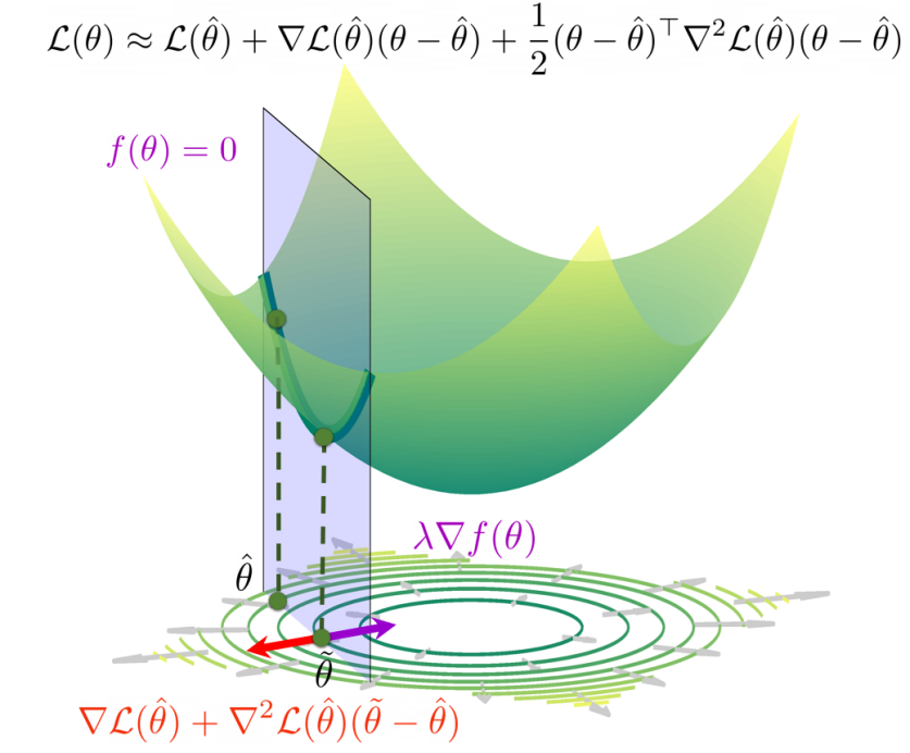
Figure 1: Geometric illustration of our Lagrangian debiasing method. The green surface is the approximation of the loss function $\mathcal{L}(\theta)$. The green circles are the contour lines of the surface. The transparent purple plane is the constraint $f(\theta)=0$. The red arrow represents $\nabla\mathcal{L}(\widehat{{\theta}})+\nabla^{2}\mathcal{L}(\widehat{{\theta}})(\widetilde{\theta}-\widehat{{\theta}})$, and the purple arrow represents $\lambda\nabla f(\theta)$.

We point out that our Lagrangian debiasing method can be applied to general inference problems beyond the BTL model. In what follows, we first present the debiasing approach for inference under general constraints. Then we provide the debiasing method under the BTL model under the special case that the constraint function $f$ is linear.

For general inferential problems under some constraint that the parameter belongs to the set $\mathcal{C}=\{{\theta}:f({\theta})=0\}$, suppose we have an initial estimator $\widehat{{\theta}}\in\mathcal{C}$, and let the loss function be $\mathcal{L}(\theta)$. By (5), if the matrix below is invertible, we define

$$\widehat{\Sigma}:=\Bigg{(}\begin{array}[]{cc}\nabla^{2}{\mathcal{L}(\widehat{{\theta}})}&\nabla{f(\widehat{{\theta}})}\\ \nabla{f(\widehat{{\theta}})}^{\top}&0\end{array}\Bigg{)}.$$ (7)

We have that the debiased estimator $\widehat{\theta}^{d}$ satisfies

$$\Bigg{(}\begin{array}[]{c}\widehat{\theta}^{d}-\widehat{\theta}\\ \lambda\end{array}\Bigg{)}=\widehat{\Sigma}^{-1}\Bigg{(}\begin{array}[]{c}-\nabla\mathcal{L}(\widehat{\theta})\\ -f(\widehat{\theta})\end{array}\Bigg{)}.$$ (8)

When the problem is high-dimensional, the matrix $\widehat{\Sigma}$ is not invertible due to the rank-deficiency, and it becomes challenging to solve problem (5). Motivated by (8), we aim to find an estimator for the inverse of the population version of $\widehat{\Sigma}$, which is

$${\Sigma}^{*}=\Bigg{(}\begin{array}[]{cc}\mathbb{E}\left[\nabla^{2}\mathcal{L}(\theta^{*})\right]&\nabla{f({{\theta}}^{*})}\\ \nabla{f({{\theta}}^{*})}^{\top}&0\end{array}\Bigg{)}.$$

We achieve this by first finding an estimator for the inverse of the population version of $\mathbb{E}\left[\nabla^{2}\mathcal{L}(\theta^{*})\right]$, and then obtain an estimator for the inverse by block matrix inverse.

Specifically, we estimate the inverse of $\mathbb{E}\left[\nabla^{2}\mathcal{L}(\theta^{*})\right]$ using the constrained $\ell_{1}$-minimization for inverse matrix estimation (CLIME) method (Cai et al. 2011). Denote the estimator as $\widehat{\Omega}$. We obtain an estimator for the inverse of $\widehat{\Sigma}$ by $\widehat{\Theta}=\Big{(}\begin{smallmatrix}\widehat{\Theta}_{11}&\widehat{\Theta}_{12}\\ \widehat{\Theta}_{12}^{\top}&\widehat{\Theta}_{22}\end{smallmatrix}\Big{)}$ where

$$\widehat{\Theta}_{11}=\widehat{\Omega}-\widehat{\Omega}\nabla{f(\widehat{{\theta}})}\big{(}\nabla{f(\widehat{{\theta}})}^{\top}\widehat{\Omega}\nabla{f(\widehat{{\theta}})}\big{)}^{-1}\nabla{f(\widehat{{\theta}})}^{\top}\widehat{\Omega},$$

and

$$\widehat{\Theta}_{12}=\widehat{\Omega}\nabla{f(\widehat{{\theta}})}\big{(}\nabla{f(\widehat{{\theta}})}^{\top}\widehat{\Omega}\nabla{f(\widehat{{\theta}})}\big{)}^{-1},\ \text{ and }\ \widehat{\Theta}_{22}=-\big{(}\nabla{f(\widehat{{\theta}})}^{\top}\widehat{\Omega}\nabla{f(\widehat{{\theta}})}\big{)}^{-1}.$$

Thus, we obtain $\widehat{\theta}^{d}$ by plugging $\widehat{\Theta}$ into (8) that

$$\Bigg{(}\begin{array}[]{c}\widehat{\theta}^{d}-\widehat{\theta}\\ \lambda\end{array}\Bigg{)}=\widehat{\Theta}\Bigg{(}\begin{array}[]{c}-\nabla\mathcal{L}(\widehat{\theta})\\ -f(\widehat{\theta})\end{array}\Bigg{)}$$ (9)

and

$$\widehat{{\theta}}^{d}=\widehat{{\theta}}-\widehat{\Theta}_{11}\nabla{\mathcal{L}({\widehat{{\theta}}})}.$$ (10)

Before presenting the asymptotic properties of $\widehat{{\theta}}^{d}$, we first impose some assumptions. We point out that here we purposely do not specify the convergence rates in the following assumptions since our proposed method is a general framework, and as long as the assumptions for Theorem 3.5 are satisfied, the Lagrangian debiased method achieves the asymptotic normality. We also point out that, under our scaling assumptions in the following theorems, the assumptions are indeed satisfied.

[Consistency for initial estimation of parameters] For some rate $r_{1}$ which depends on the sample size and parameter dimension, we assume $\big{\|}\widehat{\theta}-\theta^{*}\big{\|}_{\infty}\lesssim r_{1}$.

[Condition on loss function] For some rate $r_{2}$ and constant $L_{1}$, if $\theta={\theta}^{*}+t(\widehat{{\theta}}-{\theta}^{*})$ for $t\in[0,1]$, it holds that

$$\big{\|}\nabla\mathcal{L}({{\theta}}^{*})\|_{\infty}\lesssim r_{2},\|\nabla^{2}\mathcal{L}({{\theta}})-\nabla^{2}\mathcal{L}({{\theta}}^{*})\|_{\infty}\leq L_{1}\|{{\theta}}-{\theta}^{*}\|_{\infty}.$$

[Condition on constraint function] For some constants $c_{1}$ and $L_{2}$, if $\theta={\theta}^{*}+t(\widehat{{\theta}}-{\theta}^{*})$ for $t\in[0,1]$, it holds that

$$\big{\|}\nabla{f({{\theta}}^{*})}\big{\|}_{\infty}\lesssim c_{1},\ \|\nabla f({{\theta}})-\nabla f({{\theta}}^{*})\|_{\infty}\leq L_{2}\|{{\theta}}-{\theta}^{*}\|_{\infty}.$$

For some rates $r_{3},r_{4},r_{5}$ and constants $c_{2},c_{3}$, we assume that

$$\|I-\widehat{\Omega}\nabla^{2}{\mathcal{L}(\widehat{{\theta}})}\|_{\infty}\lesssim r_{3},\ \|\widehat{\Omega}-\Omega^{*}\|_{\infty}\lesssim r_{4},\ \big{\|}\Omega^{*}\big{\|}_{\infty}\lesssim c_{2},\ \nabla{f({{\theta}}^{*})}^{\top}\Omega^{*}\nabla{f({{\theta}}^{*})}\gtrsim c_{3},\ \big{\|}{\Theta}^{*}\big{\|}_{\infty}\lesssim r_{5}.$$

[Central limit theorem (CLT) of the score function] For every $i\neq j$, if $({\Theta}_{11}^{*}{\Sigma}_{11}^{*}{{\Theta}_{11}^{*}}^{\top})_{jj}\geq C$ and $(\bm{e}_{i}-\bm{e}_{j})^{\top}({\Theta}_{11}^{*}{\Sigma}_{11}^{*}{{\Theta}_{11}^{*}}^{\top})(\bm{e}_{i}-\bm{e}_{j})\geq C$ for some constant $C>0$, it holds that

$$\frac{\sqrt{n}\big{[}{\Theta}_{11}^{*}\nabla\mathcal{L}({{\theta}}^{*})\big{]}_{j}}{\sqrt{[{\Theta}_{11}^{*}{\Sigma}_{11}^{*}{{\Theta}_{11}^{*}}^{\top}]_{jj}}}\overset{d}{\longrightarrow}N(0,1)$$

and

$$\sqrt{n}\frac{[{\Theta}^{*}_{11}\nabla\mathcal{L}({{\theta}}^{*})]_{i}-[{\Theta}^{*}_{11}\nabla\mathcal{L}({{\theta}}^{*})]_{j}}{\sqrt{(\bm{e}_{i}-\bm{e}_{j})^{T}({\Theta}_{11}^{*}{\Sigma}_{11}^{*}{{\Theta}_{11}^{*}}^{\top})(\bm{e}_{i}-\bm{e}_{j})}}\overset{d}{\longrightarrow}N(0,1),$$

where $[{\Theta}_{11}^{*}\nabla\mathcal{L}({{\theta}}^{*})]_{j}$ is the $j$-th entry of ${\Theta}_{11}^{*}\nabla\mathcal{L}({{\theta}}^{*})$, $[{\Theta}_{11}^{*}{\Sigma}_{11}^{*}{{\Theta}_{11}^{*}}^{\top}]_{jj}$ is the $j$-th diagonal element of matrix ${\Theta}_{11}^{*}{\Sigma}_{11}^{*}{{\Theta}_{11}^{*}}^{\top}$, and ${\Sigma}_{11}^{*}$, $\Theta_{11}^{*}$ is the upper left $n\times n$ block of ${\Sigma}^{*}$, $\Theta^{*}$ respectively.

By the above assumptions, the following two corollaries hold, which are crucial for later proofs. Proofs of Corollaries 3.3 and 3.4 can be found in Section B.1 and B.2.

Corollary 3.3

Under Assumptions 1 – 3.1.1, we have $\big{\|}\widehat{\Theta}-\Theta^{*}\big{\|}_{\infty}\lesssim r_{1}+r_{4}$.

Corollary 3.4

Under Assumptions 1 – 3.1.1, we have $\|I-\widehat{\Theta}\widehat{\Sigma}\|_{\infty}\lesssim r_{3}.$

We then present the asymptotic distribution of the Lagrangian debiased estimator.

Theorem 3.5

Under Assumptions 1 – 1, if $c_{1},c_{2},c_{3},L_{1},L_{2}=\mathcal{O}(1)$ and $\sqrt{n}\big{(}r_{1}^{2}r_{5}+(r_{1}+r_{4})(r_{1}^{2}+r_{2})+r_{1}r_{3}\big{)}=o(1)$, we have the following asymptotic distribution for the Lagrangian debiased estimator (10),

$$\sqrt{n}\frac{\widehat{{\theta}}_{j}^{d}-{{\theta}}^{*}_{j}}{\sqrt{[{\Theta}_{11}^{*}{\Sigma}_{11}^{*}{{\Theta}_{11}^{*}}^{\top}]_{jj}}}\overset{d}{\longrightarrow}N(0,1),$$

and

$$\sqrt{n}\frac{(\widehat{{\theta}}_{i}^{d}-{{\theta}}^{*}_{i})-(\widehat{{\theta}}_{j}^{d}-{{\theta}}^{*}_{j})}{\sqrt{(\bm{e}_{i}-\bm{e}_{j})^{\top}{\Theta}_{11}^{*}{\Sigma}_{11}^{*}{{\Theta}_{11}^{*}}^{\top}(\bm{e}_{i}-\bm{e}_{j})}}\overset{d}{\longrightarrow}N(0,1),$$

where $\bm{e}_{k}$ is the natural basis with the $k$-th entry be 1 and other entries be 0.

Proof 3.6

See Appendix Section A.1 for the detailed proof.

Remark 3.7

If the constraint function $f$ is linear, it is not difficult to say that $\widehat{\theta}^{d}$ satisfies the constraint. Meanwhile, under the general constraint, as the problem is nonconvex, $\widehat{\theta}^{d}$ may violate the constraint. However, even if the constraint is violated, the asymptotic results above still hold.

3.1.2 Lagrangian Debiasing for BTL model

We present the debiasing method under the BTL model. In particular, for ranking problems, letting the constraint function be linear that $\bm{1}^{\top}{\theta}=0$ as in Chen et al. (2013), Negahban et al. (2017), Jin et al. (2020), we define

$$\Bigg{(}\begin{array}[]{cc}\widehat{\Theta}_{11}&\frac{1}{n}\mathbf{1}\\ \frac{1}{n}\mathbf{1}^{\top}&0\end{array}\Bigg{)}=\Bigg{(}\begin{array}[]{cc}\nabla^{2}\mathcal{L}(\widehat{\theta})&\mathbf{1}\\ \mathbf{1}^{\top}&0\end{array}\Bigg{)}^{-1}\text{ and }\Bigg{(}\begin{array}[]{cc}\Theta^{*}_{11}&\frac{1}{n}\mathbf{1}\\ \frac{1}{n}\mathbf{1}^{\top}&0\end{array}\Bigg{)}=\Bigg{(}\begin{array}[]{cc}\nabla^{2}\mathcal{L}(\theta^{*})&\mathbf{1}\\ \mathbf{1}^{\top}&0\end{array}\Bigg{)}^{-1}$$ (11)

Here the invertibility is provied in Remark H.9 in the Appendix, and the form of inverse is validated in Corollary H.10.

The next theorem shows that under mild scaling conditions, the Lagrangian debiasing estimator $\widehat{\theta}^{d}_{j}$ and the component-wise difference ${\widehat{\theta}^{d}}_{i}-{\widehat{\theta}^{d}}_{j}$ for any $i$ and $j$ ($1\leq i,j\leq n$) are asymptotically normal with mean $\theta^{*}_{j}$ and ${{\theta}}^{*}_{i}-{{\theta}}^{*}_{j}$, respectively.

Theorem 3.8

Considering the BTL model, under constraint parameter set $\mathcal{C}=\{{\theta}:\bm{1}^{\top}{\theta}=0\}$, if $p\geq\frac{C_{0}\log n}{n}$ for some sufficiently large constant $C_{0}>0$ and $\frac{n\log n}{\sqrt{L}}+\frac{\log n}{\sqrt{pL}}=o(1)$, we have that the Lagrangian debiasing estimator satisfies that, as $n,L\rightarrow\infty$,

$$\sqrt{L}\ \dfrac{\widehat{\theta}^{d}_{j}-{\theta}_{j}^{*}}{\sqrt{[{\Theta_{11}^{*}}]_{jj}}}\overset{d}{\longrightarrow}N(0,1),$$

and

$$\sqrt{L}\frac{{\widehat{\theta}^{d}}_{i}-{\widehat{\theta}^{d}}_{j}-({{\theta}}^{*}_{i}-{{\theta}}^{*}_{j})}{\sqrt{(\bm{e}_{i}-\bm{e}_{j})^{\top}{\Theta_{11}^{*}}(\bm{e}_{i}-\bm{e}_{j})}}\overset{d}{\longrightarrow}N(0,1).$$

Proof 3.9

See Appendix A.2 for the detailed proof.

Remark 3.10

By Corollary H.10 in the Appendix, we have that $[{\Theta_{11}^{*}}]_{jj}\asymp\frac{1}{np}\text{ for all }1\leq j\leq n$. Consequently, for all $j\in[n]$, we have

$$\big{|}\widehat{\theta}^{d}_{j}-{\theta}_{j}^{*}\big{|}\lesssim\sqrt{\frac{1}{npL}}$$

with probability goes to 1. This matches the $\ell_{\infty}$-norm error achieved by the spectral and regularized MLE methods as analyzed in (Chen et al. 2019).

The asymptotic normality of ${\widehat{\theta}^{d}}_{i}-{\widehat{\theta}^{d}}_{j}$ is the fundamental building block for inferring the pairwise preference such as in Example 1.1, where we test if item $i$ is preferred over item $j$. Basically, it is a “local” test that only involves two items, which can be done with the asymptotic distribution of ${\widehat{\theta}^{d}}_{i}-{\widehat{\theta}^{d}}_{j}$. For the more challenging “global” testing problems, such as Example 1.2, where we test if a given item is among the top-$K$ ranked items, we need to uniformly control the quantile of maximal statistic, which will be discussed in the next subsection.

3.2 Hypothesis Testing

In this subsection, we propose our general inferential framework for ranking problems. As mentioned in the Introduction, we first test if a given item $i$ satisfies some property that

$$H_{0}:\gamma^{*}\notin\mathcal{R}_{i}\text{ \ \ v.s. \ \ }H_{a}:\gamma^{*}\in\mathcal{R}_{i}.$$

To facilitate our discussion, we define the legal pair and a distance between the null and alternative, which essentially measure the signal strengths in our testing problems. In particular, when we test some property of item $i$, we say a pair $(i,i^{\prime})$ is a legal pair if the property is true, and if we swap the scores of item $i$ and item $i^{\prime}$, the property no longer holds. That is, swapping the scores of item $i$ and item $i^{\prime}$ changes the property of our interest. The distance between the null and alternative is thus defined as the minimal difference of scores among all legal pairs.

Definition 3.11 (Legal pair)

Suppose $\gamma\in\mathcal{R}_{i}$. After swapping the scores of item $i$ and item $i^{\prime}$, we obtain a new rank $\gamma^{\prime}$. We say that the pair of items $(i,i^{\prime})$ is legal if $\gamma^{\prime}\notin\mathcal{R}_{i}$.

Definition 3.12 (Distance between the null and alternative)

We define the distance between the null and alternative as

$$\Delta({\theta},\mathcal{R}_{i})=\min_{i^{\prime}:(i,i^{\prime})\text{ is legal }}|\theta_{i}-\theta_{i^{\prime}}|.$$

Then, we provide the specific legal pairs and distances $\Delta({\theta},\mathcal{R}_{i})$ for Examples 1.1 and 1.2.

• Example 1.1: (Pairwise preference between item $i$ and item $j$). We aim to test if item $i$ is ranked higher than item $j$, which means $\gamma^{*}_{i}<\gamma^{*}_{j}$ or $\theta^{*}_{i}>\theta^{*}_{j}$. Let the ranking property be

  $$\mathcal{R}_{i}=\{\gamma:\gamma_{i}<\gamma_{j}\}=\{\gamma(\theta):\theta_{i}>\theta_{j}\}.$$

  If $\gamma\in\mathcal{R}_{i}$ (i.e., $\theta_{i}>\theta_{j}$) and we swap scores of item $i$ and item $i^{\prime}$ where $\theta_{i^{\prime}}\leq\theta_{j}$, the new rank does not satisfy $\mathcal{R}_{i}$. Meanwhile, if we swap scores of item $i$ and item $i^{\prime\prime}$ where $\theta_{i^{\prime\prime}}>\theta_{j}$, the new rank still satisfies $\mathcal{R}_{i}$. So $(i,i^{\prime})$ is a legal pair if $\theta_{i^{\prime}}\leq\theta_{j}$. See Figure 2 for illustration. This observation leads to the distance

  $$\Delta({\theta},\mathcal{R}_{i})=\min_{i^{\prime}:\theta_{i^{\prime}}\leq\theta_{j}}|\theta_{i}-\theta_{i^{\prime}}|=|\theta_{i}-\theta_{j}|.$$

  Equivalently, we can test on preference scores instead of ranking, i.e., testing whether item $i$ has a larger score than item $j$,

  $$H_{0}:\theta^{*}_{i}\leq\theta^{*}_{j}\text{\ \ v.s.\ \ }H_{a}:\theta^{*}_{i}>\theta^{*}_{j}.$$

  Figure 2: Illustration of Example 1.1. Assuming $\theta_{1}>\theta_{2}>\cdots>\theta_{n}$. Here $\gamma\in\mathcal{R}_{i}$ since $\theta_{i}>\theta_{j}$. If we swap scores of item $i$ and item $i^{\prime}$ where $\theta_{i^{\prime}}\leq\theta_{j}$, the new rank does not satisfy $\mathcal{R}_{i}$. Meanwhile, if we swap scores of item $i$ and item $i^{\prime\prime}$ where $\theta_{i^{\prime\prime}}>\theta_{j}$, the new rank still satisfies $\mathcal{R}_{i}$. Thus, $(i,i^{\prime})$ is a legal pair if $\theta_{i^{\prime}}\leq\theta_{j}$.

• Example 1.2: (Top-$K$ test). If item $i$’s preference score is larger than $n-K$ items, i.e., $\theta_{i}>\theta_{(K+1)}$, where $\theta_{(K+1)}$ denotes the $(K+1)$-th largest preference score, or equivalently, $\gamma_{i}\leq K$, we say that item $i$ is ranked among top-$K$ items. We aim to test if item $i$ is ranked among top-$K$ items. Thus, we have that $\mathcal{R}_{i}$ is

  $$\mathcal{R}_{i}=\{\gamma:\gamma_{i}\leq K\}=\{\gamma(\theta):\theta_{i}>\theta_{(K+1)}\}.$$

  If $\gamma\in\mathcal{R}_{i}$ (i.e., $\theta_{i}>\theta_{(K+1)}$), and we swap scores of item $i$ and item $j$ where $\theta_{j}\leq\theta_{(K+1)}$, the new rank does not satisfy $\mathcal{R}_{i}$. Meanwhile, if we swap scores of item $i$ and item $j$ where $\theta_{j}>\theta_{(K+1)}$, we have that the new rank satisfies $\mathcal{R}_{i}$. Thus, $(i,j)$ is a leagal pair if $\theta_{j}\leq\theta_{(K+1)}$, and the distance is

  $$\Delta({\theta},\mathcal{R}_{i})=\min_{j:\theta_{j}\leq\theta_{(K+1)}}|\theta_{i}-\theta_{j}|=|\theta_{i}-\theta_{(K+1)}|.$$

  Similarly, we can transform the test on ranking into testing on preference score, our test is

  $$H_{0}:\theta^{*}_{i}-\theta^{*}_{(K+1)}\leq 0\text{\ \ v.s.\ \ }H_{a}:\theta^{*}_{i}-\theta^{*}_{(K+1)}>0.$$

Next, we explain our testing procedure with the above two examples. Consider Example 1.1, where we test if item $i$ is ranked higher than item $j$, or equivalently, we test if item $i$ has a larger score than item $j$,

$$H_{0}:\theta^{*}_{i}\leq\theta^{*}_{j}\text{\ \ v.s.\ \ }H_{a}:\theta^{*}_{i}>\theta^{*}_{j}.$$

For this example, by Theorem 3.8, if the assumptions are satisfied, we have

$$\sqrt{L}\frac{{\widehat{\theta}^{d}}_{i}-{\widehat{\theta}^{d}}_{j}-({{\theta}}^{*}_{i}-{{\theta}}^{*}_{j})}{\sqrt{(\bm{e}_{i}-\bm{e}_{j})^{\top}{\Theta_{11}^{*}}(\bm{e}_{i}-\bm{e}_{j})}}\overset{d}{\longrightarrow}N(0,1).$$

We thus reject $H_{0}$ if

$$\sqrt{L}\frac{\widehat{\theta}^{d}_{i}-\widehat{\theta}^{d}_{j}}{\sqrt{(\bm{e}_{i}-\bm{e}_{j})^{\top}{\widehat{\Theta}_{11}}(\bm{e}_{i}-\bm{e}_{j})}}>\Phi(1-\alpha),$$

where $\Phi(\cdot)$ is the cumulative distribution function of a standard normal random variable.

Note that this example only involves two items, which is a relatively simple local test. However, for more general testing problems, we need to consider more than two items. For instance, in Example 1.2, we test if item $i$ is ranked among the top-$K$ items that

$$H_{0}:\theta^{*}_{i}-\theta^{*}_{(K+1)}\leq 0\text{\ \ v.s.\ \ }H_{a}:\theta^{*}_{i}-\theta^{*}_{(K+1)}>0.$$

where $\theta^{*}_{(K+1)}$ is the $(K+1)$-th largest score in terms of order statistic. If the score of item $i$ is larger than the $(K+1)$-th largest score, we have that item $i$ is ranked among top-$K$ items. In this example and more general problems, we need to study the maximal statistic $\max_{j\neq i}(\widehat{\theta}^{d}_{i}-\theta^{*}_{i}-\widehat{\theta}^{d}_{j}+\theta^{*}_{j})$. In what follows, we demonstrate that we can estimate the quantiles of this maximal statistic via the Gaussian multiplier bootstrap.

Gaussian multiplier bootstrap. We start from a general fixed edge set $E\subseteq\mathcal{V}\times\mathcal{V}$. The goal is to control the tail probability of the statistic that

$$T:= \max_{(i,j)\in E}\sqrt{{npL}}(\widehat{\theta}^{d}_{i}-\theta^{*}_{i}-\widehat{\theta}^{d}_{j}+\theta^{*}_{j})$$ (12)

$$= -\max_{(i,j)\in E}\sqrt{\frac{1}{npL}}\sum_{\ell=1}^{L}\sum_{k>m}{\mathcal{E}_{mk}}\Big{(}-y_{mk}^{(\ell)}+\frac{e^{\theta_{k}^{*}}}{e^{\theta_{k}^{*}}+e^{\theta_{m}^{*}}}\Big{)}np\big{(}[{\Theta}^{*}_{11}]_{i}-[{\Theta}^{*}_{11}]_{j}\big{)}(\bm{e}_{k}-\bm{e}_{m})$$

$$+\sqrt{{npL}}(r_{i}-r_{j})$$

$$:= \max_{(i,j)\in E}\sqrt{\frac{1}{L}}\sum_{\ell=1}^{L}x_{ij}^{(\ell)}+\sqrt{{npL}}(r_{i}-r_{j}),$$

where $\bm{e}_{k}$ is the natural basis, $[{\Theta_{11}^{*}}]_{i}$ is the $i$-th row of matrix ${\Theta_{11}^{*}}$ defined in (11). The second equality comes from (41) and (33). $x_{ij}^{(\ell)}$ is defined as

$$x_{ij}^{(\ell)}:=-\sqrt{{np}}\sum_{k>m}{\mathcal{E}_{mk}}\Big{(}-y_{mk}^{(\ell)}+\frac{e^{\theta_{k}^{*}}}{e^{\theta_{k}^{*}}+e^{\theta_{m}^{*}}}\Big{)}\big{(}[{\Theta_{11}^{*}}]_{i}-[{\Theta_{11}^{*}}]_{j}\big{)}(\bm{e}_{k}-\bm{e}_{m}).$$ (13)

which is an independent zero-mean random variable in $\mathbb{R}$ for $\ell=1,\cdots,L$. Here $\mathcal{E}_{mk}=1$ if $(m,k)\in\mathcal{E}$ the comparison graph, and $\mathcal{E}_{mk}=0$ otherwise.

To estimate the quantile of $T$, we consider the Gaussian multiplier bootstrap in Chernozhukov et al. (2013). The main idea is to approximate the distribution of the maximum of a sum of independent random vectors with unknown covariance by the distribution of the maximum of a sum of conditional Gaussian random vectors, which is obtained by multiplying the original vectors with i.i.d. normal random variables. In our case, even though vector ${\theta}^{*}$ is not observable, we have some estimators $\widehat{{\theta}}$ are available, and we use the estimators to approximate ${\theta}^{*}$ in the bootstrap.

Hence, we define the following statistic from Gaussian multiple bootstrap

$$W:=\max_{(i,j)\in E}\sqrt{\frac{1}{L}}\sum_{\ell=1}^{L}\bigg{\{}-\sqrt{{np}}\sum_{k>m}{\mathcal{E}_{mk}}\Big{(}-y_{mk}^{(\ell)}+\frac{e^{\widehat{\theta}_{k}}}{e^{\widehat{\theta}_{k}}+e^{\widehat{\theta}_{m}}}\Big{)}\big{(}[\widehat{\Theta}_{11}]_{i}-[\widehat{\Theta}_{11}]_{j}\big{)}(\bm{e}_{k}-\bm{e}_{m})\bigg{\}}z_{\ell},$$ (14)

where $z_{\ell}$, $\ell=1,\cdots,L$, are i.i.d standard normal random variables.

We then estimate the conditional quantile of $W$ given data $\bm{y}=\big{\{}y_{mk}^{(\ell)}\big{\}}^{\ell=1,\cdots,L}_{k>m}$ by

$$c_{W}(\alpha,E)=\inf\big{\{}t\in\mathbb{R}:\mathbb{P}(W>t{\,|\,}\bm{y})\leq\alpha\big{\}}.$$ (15)

The next theorem uniformly controls the tail probability of $T$ by $c_{W}(\alpha,E)$.

Theorem 3.13

Considering the BTL model, for any edge set $E\subseteq\mathcal{V}\times\mathcal{V}$, if $n^{2}p\frac{(\log(nL))^{7}}{L}=o(1)$ and $\frac{n(\log n)^{3/2}}{\sqrt{L}}=o(1)$, we have

$$\sup_{\alpha\in(0,1)}\big{|}\mathbb{P}(T>c_{W}(\alpha,E))-\alpha\big{|}\to 0.$$

as $n,L\to\infty$,

Proof 3.14

We provide the proof in Appendix Section D.

This theorem shows that $c_{W}(\alpha,E)$ obtained from the Gaussian multiplier bootstrap is a valid quantile estimator for $T=\max_{i,j\in E}\sqrt{{npL}}(\widehat{\theta}^{d}_{i}-\theta^{*}_{i}-\widehat{\theta}^{d}_{j}+\theta^{*}_{j})$. In this theorem, the first scaling condition $n^{2}p\frac{(\log(nL))^{7}}{L}=o(1)$ is from the Gaussian approximation for the maximum of a sum of random vectors, and the second scaling condition $\frac{n(\log n)^{3/2}}{\sqrt{L}}=o(1)$ is from approximating $T$ and $W$ by their leading terms. Given this statistic, we are ready to present the procedure for testing general ranking properties.

General testing procedure. For general ranking property test with respect to item $i$

$${H}_{0}:\gamma^{*}\notin\mathcal{R}_{i}\text{ \ \ v.s. \ \ }{H}_{a}:\gamma^{*}\in\mathcal{R}_{i},$$

we perturb the preference score of every item (i.e., $\widehat{\theta}^{d}_{i}$) up to $\alpha$-quantile of $\max_{j\neq i}(\widehat{\theta}^{d}_{i}-\theta^{*}_{i}-\widehat{\theta}^{d}_{j}+\theta^{*}_{j})$, and conduct the test. Specifically, let $\widetilde{\Theta}$ be the set of all possible score vectors after perturbation that

$$\widetilde{\Theta}=\Big{\{}{\theta}:{\theta}_{k}\in\big{[}\widehat{\theta}^{d}_{k}-c_{W}(\alpha,i)/\sqrt{npL},\ \widehat{\theta}^{d}_{k}+c_{W}(\alpha,i)/\sqrt{npL}\big{]},1\leq k\leq n\Big{\}}.$$ (16)

We reject the null hypothesis if $\gamma{({\theta})}\in\mathcal{R}_{i}$ for any ${\theta}\in\widetilde{\Theta}$, i.e., the event $\cap_{{\theta}\in\widetilde{\Theta}}\{\gamma{({\theta})}\in\mathcal{R}_{i}\}$ holds.

Remark 3.15

We point out that we can simplify this general procedure for specific problems. For instance, when we test if item $i$ is ranked within the top-$K$, we only need to consider the extreme point of the perturbation, where for $k=1,...,n$, its $k$-th entry is defined as

$$\theta_{k}=\left\{\begin{array}[]{ll}\widehat{\theta}^{d}_{k}&\quad\widehat{\theta}^{d}_{k}>\widehat{\theta}^{d}_{i},\\ \widehat{\theta}^{d}_{k}-c_{W}(\alpha,i)/\sqrt{npL}&\quad k=i,\\ \widehat{\theta}^{d}_{k}+c_{W}(\alpha,i)/\sqrt{npL}&\quad\widehat{\theta}^{d}_{k}<\widehat{\theta}^{d}_{i}.\end{array}\right.$$

In fact, we can further simplify this procedure that we only consider ${\theta}$ where its $k$-th entry is defined as

$$\theta_{k}=\left\{\begin{array}[]{ll}\widehat{\theta}^{d}_{k}&\quad\widehat{\theta}^{d}_{k}>\widehat{\theta}^{d}_{i},\\ \widehat{\theta}^{d}_{k}-c_{W}(\alpha,i)/\sqrt{npL}&\quad k=i,\\ \widehat{\theta}^{d}_{k}&\quad\widehat{\theta}^{d}_{k}<\widehat{\theta}^{d}_{i}.\end{array}\right.$$

We justify this procedure in Appendix Section E.2.

We conclude this section by the following theorem that we show that the proposed procedure controls the Type I error, and we provide the power analysis.

Theorem 3.16

Under same assumptions as in Theorem 3.8 and 3.13, we have the general testing procedure satisfies that, as $n,L\to\infty$,

$$\sup_{\gamma^{*}\notin\mathcal{R}_{i}}\mathbb{P}_{0}\left(\text{Reject }H_{0}\right)\leq\alpha,$$

and we have

$$\inf_{\gamma^{*}\in\mathcal{R}_{i},\Delta({\theta}^{*},\mathcal{R}_{i})>\delta}\mathbb{P}\left(\text{Reject }H_{0}\right)\to 1,$$

where $\delta=C\sqrt{\frac{\log n}{npL}}$ for some constant $C$.

Proof 3.17

We provide the proof in Appendix Section E.

4 Multiple Testing

In this section, we extend the proposed procedure to the multiple testing setting. As discussed in the introduction, the multiple testing finds important applications in our ranking inference problems such as Example 1.3, where we aim to infer the set of all top-$K$ ranked items. In general multiple testing problems, we aim to control the familywise Type I error rate (FWER), or the false discovery rate (FDR), while achieving certain power. Widely used procedures include Bonferroni correction, Dunn-Šidák procedure (Šidák 1967), Holm Procedure (Holm 1979) for controlling FWER, and Benjamini-Hochberg procedure (BH) (Benjamini and Hochberg 1995), Benjamini-Yekutieli procedure (Benjamini and Yekutieli 2001) for controlling FDR. In addition, there are also resampling based procedures such as permutation testing and bootstrap method (Westfall and Young 1993, Ge et al. 2003). However, these methods cannot be directly applied to our problems, as their theoretical properties cannot be easily justified. This is mainly because that the test statistics for the hypotheses are clearly dependent, which makes our multiple testing problems challenging.

In general, we aim to test the following hypotheses simultaneously,

$$H_{0i}:\text{item }i\text{ does not satisfy property }\mathcal{R}_{i}\text{\ \ v.s.\ \ }H_{ai}:\text{item }i\text{ satisfies }\mathcal{R}_{i},\text{\ \ \ for }i\in[n].$$ (17)

4.1 Control FWER

We first present our procedure for controlling the FWER. Recall that the FWER is the probability of making at least one Type I error that

$$\text{FWER}=\mathbb{P}(\char 35\relax\text{ false positives}>0).$$

Specifically, when we aim to control the FWER in multiple testing, we let the maximal statistic be

$$M=\max_{i\in[n]}\max_{j\in[n]}\sqrt{{npL}}(\widehat{\theta}^{d}_{i}-\theta^{*}_{i}-\widehat{\theta}^{d}_{j}+\theta^{*}_{j}),$$

and we estimate its $(1-\alpha)$-th percentile $C_{M}(\alpha,[n]\times[n])$ by Gaussian multiplier bootstrap and taking the edge set $E$ as $[n]\times[n]$ in (12). Next, we reject the $H_{0i}$ in (17) if item $i$ satisfies property $\mathcal{R}_{i}$ for all possible perturbation for the debiased estimator $\widehat{\theta}^{d}$ up to $C_{M}(\alpha,[n]\times[n])/\sqrt{npL}$ entrywise. Equivalently, letting $\widetilde{\Theta}$ be the set of possible latent scores after perturbation that

$$\widetilde{\Theta}=\Big{\{}{\theta}:{\theta}_{k}\in\big{[}\widehat{\theta}^{d}_{k}-C_{M}(\alpha,[n]\times[n])/\sqrt{npL},\ \widehat{\theta}^{d}_{k}+C_{M}(\alpha,[n]\times[n])/\sqrt{npL}\big{]},1\leq k\leq n\Big{\}},$$

we reject $H_{0i}$ in (17) if for any ${\theta}\in\widetilde{\Theta}$, we have $\gamma{({\theta})}\in\mathcal{R}_{i}$, i.e., the event $\cap_{{\theta}\in\widetilde{\Theta}}\{\gamma{({\theta})}\in\mathcal{R}_{i}\}$ holds.

To facilitate our power analysis, we define the signal strength for multiple testing problems as

$$\Delta({\theta})=\min_{i:\gamma(\theta)\in\mathcal{R}_{i}}\Delta({\theta},\mathcal{R}_{i})=\min_{i:\gamma(\theta)\in\mathcal{R}_{i}}\min_{i^{\prime}:(i,i^{\prime})\text{ is legal }}|\theta_{i}-\theta_{i^{\prime}}|.$$ (18)

In what follows, we use two examples to illustrate some insights of this signal strength.

• Consider the problem of selecting all top-$K$ ranked items. Denote the $i$-th largest order statistic as $\theta_{(i)}$. For any given $1\leq i\leq n$ satisfying $\theta_{i}\geq\theta_{(K)}$, the pairs of items $(i,i^{\prime})$ such that $\theta_{i^{\prime}}\leq\theta_{(K+1)}$ are the legal pairs, and the smallest distance is $|\theta_{i}-\theta_{(K+1)}|$. Hence, we have

  $$\Delta({\theta})=\min_{\theta_{i}\geq\theta_{(K)}}\min_{\theta_{i^{\prime}}\leq\theta_{(K+1)}}|\theta_{i}-\theta_{i^{\prime}}|=\min_{\theta_{i}\geq\theta_{(K)}}|\theta_{i}-\theta_{(K+1)}|=|\theta_{(K)}-\theta_{(K+1)}|.$$

  This is consistent with our intuition that when we aim to choose the top $K$ items, the gap between the scores of $\theta_{(K)}$ and $\theta_{(K+1)}$ somewhat determines this problem’s difficulty.

• Consider the problem of selecting all items ranked higher than item $k$ with score $\theta_{k}$. For any item $i$ satisfying $\theta_{i}>\theta_{k}$, the pairs $(i,i^{\prime})$ where $\theta_{i^{\prime}}\leq\theta_{k}$ are legal pairs. Hence, we have that the distance is

  $$\Delta({\theta})=\min_{\theta_{i}>\theta_{k}}\min_{\theta_{i}^{\prime}\leq\theta_{k}}|\theta_{i}-\theta_{i^{\prime}}|=\min_{\theta_{i}>\theta_{k}}|\theta_{i}-\theta_{k}|.$$

The following theorem shows that the FWER based on our procedure above is guaranteed to be no greater than $\alpha$ asymptotically and is powerful.

Theorem 4.1 (Familywise Type I Error Rate)

Under the same assumptions for Theorems 3.8 and 3.13, following the multiple testing procedure above, for any $0<\alpha<0.5$, we have

$$\mathrm{FWER}=\mathbb{P}(\text{Making at least one Type I error})\leq\alpha+o(1).$$

Further, if $\Delta({\theta}^{*})\gtrsim\sqrt{\frac{\log n}{npL}}$ holds, we have

$$\mathbb{P}(\text{Making at least one Type II error})\to 0.$$

Proof 4.2

We provide the proof in Appendix Section F.1.

This theorem shows that our method controls the FWER asymptotically for the given level. Meanwhile, our procedure is asymptotically powerful if $\Delta({\theta}^{*})\gtrsim\sqrt{\frac{\log n}{npL}}$, which matches the lower bound we derive in Section 5.

4.2 FDR Control

We then consider the problem of controlling the false discovery rate (FDR). FDR is the expected proportion of Type I errors among the all discoveries (Benjamini and Hochberg 1995), and our goal is to control the FDR under some prespecified level $\alpha$ that

$$\text{FDR}=\mathbb{E}\Big{[}\frac{\char 35\relax\text{ false positives }}{\char 35\relax\text{ discoveries }}\mathbb{I}[\ \char 35\relax\text{ discoveries }>0]\Big{]}\leq\alpha.$$

Consider the multiple testing problem of our interest (17). For each hypothesis of item $i$, we perform our proposed single testing procedure in Section 3.2 and get the p-value $p_{i}$ that

$$p_{i}=\inf\big{\{}\alpha_{0}:\cap_{{\theta}\in\widetilde{\Theta}(\alpha_{0})}\{\gamma{({\theta})}\in\mathcal{R}_{i}\}\big{\}}\ \ \text{for }1\leq i\leq n,$$

where

$$\widetilde{\Theta}(\alpha_{0})=\Big{\{}{\theta}:{\theta}_{k}\in\big{[}\widehat{\theta}^{d}_{k}-c_{W}(\alpha_{0},i)/\sqrt{npL},\ \widehat{\theta}^{d}_{k}+c_{W}(\alpha_{0},i)/\sqrt{npL}\big{]},1\leq k\leq n\Big{\}}.$$

Since the p-values $p_{i}$’s for different tests have complicated dependency, we consider the Benjamini-Yekutieli procedure by Benjamini and Yekutieli (2001) to control the FDR, which ranks the hypotheses according to their corresponding p-values and chooses a cutoff to control the FDR. In particular, we order the $n$ p-values in the ascending order as $p_{(1)},\cdots,p_{(n)}$ and reject the null hypothesis for all $H_{(i)}$, $i=1,\ldots,r$, where

$$r=\max_{k}\Big{\{}k:p_{(k)}\leq\frac{k}{n\cdot N}\cdot\alpha\Big{\}}\text{ \ \ and \ \ }N=\sum_{k=1}^{n}\frac{1}{k}.$$

The following theorem shows that the FDR based on our procedure achieves the desired FDR level asymptotically if $|\mathcal{H}_{0}|\Big{(}\frac{1}{L^{c_{3}}}+\frac{2}{n^{5}}\Big{)}=o(1)$, where $|\mathcal{H}_{0}|$ is the number of true null hypotheses.

Theorem 4.3 (FDR control)

Suppose that the conditions in Theorems 3.8 and 3.13 hold. Following the multiple testing procedure above, for any $0<\alpha<1$, we have

$$\text{FDR}\leq\frac{|\mathcal{H}_{0}|}{n}\cdot\alpha+C|\mathcal{H}_{0}|\Big{(}\frac{1}{L^{c_{3}}}+\frac{2}{n^{5}}\Big{)},$$

for some constant $C>0$, and the constant $c_{3}$ satisfies the condition in Remark D.2.

Proof 4.4

We provide the proof in Appendix Section F.2.

Remark 4.5

We point out that, as show in the theorem above and in our simulation studies, our developed B-Y based FDR controlling procedure is relatively conservative when the number of true nulls $|\mathcal{H}_{0}|$ is small compared to total number of items $n$. The similar conservative result also holds in Eisenach et al. (2020).

5 Lower Bound Theory

In this section, we derive a lower bound for the multiple testing problem (17). To the best of our knowledge, even beyond ranking problems, all existing works focus on discussing the lower bound for single hypothesis testing problems. To facilitate our discussion, we first define a novel minimax risk of multiple testing problems. In particular, we let the risk be the probability of making at least one Type I or Type II error that

$$\mathfrak{R}=\inf_{\psi}\sup_{\theta^{*}\in\Xi}{\mathbb{P}}(\char 35\relax\text{ false positives}+\char 35\relax\text{ false negatives }\geq 1),$$ (19)

where $\psi$ is any selection procedure giving a vector $\psi\in\{0,1\}^{n}$ that $\psi_{i}=1$ means that we reject $H_{0i}$ in (17), and $\Xi$ is our parameter space, which is closed under swapping scores of any two items. If $\mathfrak{R}\geq 1-\epsilon$, where $\epsilon>0$ is a constant, we say that any procedure fails in the sense that Type I or Type II error can not be controlled. Given this setup, we aim to characterize necessary conditions under which we can control the minimax risk to the desired level.

5.1 Lower Bound Theorem

Recall that we define the legal pair in Definition 3.11 and the distance $\Delta({\theta})$ in (18). We then define a critical subset of all legal pairs, which is crucial in deriving the information-theoretic lower bound and captures the “hardness” of multiple testing for different properties.

Definition 5.1 (Divider set)

A set $\mathcal{M}(\theta)\subseteq[n]\times[n]$ is a divider set if $\mathcal{M}(\theta)$ satisfies the following two conditions,

• For any $(i,i^{\prime})\in\mathcal{M}(\theta)$, it satisfies $\gamma\in\mathcal{R}_{i}$, $(i,i^{\prime})$ is legal, and $|\theta_{i}-\theta_{i^{\prime}}|=\Delta({\theta})$.

• For any two pairs $(i_{1},i_{1}^{\prime}),(i_{2},i_{2}^{\prime})\in\mathcal{M}(\theta)$, letting $\gamma_{1}$ be the scores by swapping items $i_{1}$ and $i^{\prime}_{1}$, and $\gamma_{2}$ be the scores by swapping items of $i_{2}$ and $i^{\prime}_{2}$. They must satisfy $\{i:\gamma_{1}\in\mathcal{R}_{i}\}\neq\{i:\gamma_{2}\in\mathcal{R}_{i}\}$.

The following theorem derives necessary signal strengths in $\Delta(\theta)$ and $|\mathcal{M}(\theta)|$ for controlling the risk $\mathfrak{R}\leq 1-\epsilon$.

Theorem 5.2 (Necessary Signal Strength)

Considering the BTL model where the pairwise comparison probability $p$ in Erdös-Rényi graph satisfies $p\gtrsim\frac{\log n}{n}$, if there exists $\theta\in\Xi$ such that

$$\Delta({\theta})\lesssim\sqrt{\frac{\epsilon\log\big{(}|\mathcal{M}(\theta)|+1\big{)}-\log 2}{npL}},$$ (20)

we have the minimax risk $\mathfrak{R}=\inf_{\psi}\sup_{\theta^{*}\in\Xi}{\mathbb{P}}(\char 35\relax\text{ false positives}+\char 35\relax\text{ false negatives }\geq 1)>1-\epsilon$.

Proof 5.3

Our proof is based on three steps. In the first step, we reduce the problem of obtaining a lower bound of minimax risk in (19) for $\theta^{*}\in\Xi$ to the problem of deriving a lower bound for $\theta^{*}$ in a finite set. Next, we construct a finite set of hypotheses. Finally, we derive the minimax risk by Fano-type arguments, and derive the necessary signal strength condition.

Step 1. Let $\mathcal{R}_{j}$ be a ranking property for a single item $j$ as defined in Definition 2.3. We have

$$\mathfrak{R} =\inf_{\psi}\sup_{\theta^{*}\in\Xi}{\mathbb{P}}(\char 35\relax\text{ false positives}+\char 35\relax\text{ false negatives }\geq 1)$$ (21)

$$=\inf_{\psi}\sup_{\theta^{*}\in\Xi}{\mathbb{P}}(\psi\neq\psi^{*})=\inf_{\psi}\sup_{\theta^{*}\in\Xi}{\mathbb{P}}(d(\psi,\psi^{*})\geq 1/2),$$

where $\psi^{*}\in\{0,1\}^{n}$ with $\psi^{*}_{j}=1$ meaning $\gamma^{*}\in\mathcal{R}_{j}$ and $\psi^{*}_{j}=0$ meaning $\gamma^{*}\notin\mathcal{R}_{j}$ for $j=1,\cdots,n$, and $\psi\in\{0,1\}^{n}$ is a selection procedure that $\psi_{i}=1$ means that we reject $H_{0i}$ in (17), and the distance $d(\psi,\psi^{*})=\|\psi-\psi^{*}\|_{1}$. By Section 2.2 of Tsybakov (2008), the problem of obtaining a lower bound of minimax risk in (21) for $\theta^{*}\in\Xi$ can be reduced to the problem of deriving a lower bound for $\theta^{*}$ in a finite set. In particular, suppose that we have a collection $M+1$ hypotheses $\mathcal{H}_{M}=\{H_{i}:\theta^{*}=\theta^{(i)},0\leq i\leq M\}$. Recall that a test is any measurable function $\phi:\bm{Y}=\{\bm{Y}^{(\ell)}\}_{\ell=1}^{L}\mapsto\{0,1,\cdots,M\}$. Let $\mathbb{P}_{e,M}$ be the minimax probability of error

$$\mathbb{P}_{e,M}:=\inf_{\phi}\max_{\theta^{*}\in\{\theta^{(0)},\theta^{(1)},\cdots,\theta^{(M)}\}}\mathbb{P}_{i}(\phi\neq i)=\inf_{\phi}\max_{0\leq i\leq M}\mathbb{P}_{i}(\phi\neq i),$$ (22)

where $\mathbb{P}_{i}$ denotes the probability measure under the $i$-th hypothesis $\theta^{*}=\theta^{(i)}$. The following lemma in Section 2.2 of Tsybakov (2008) shows that the minimax risk $\mathfrak{R}$ in (21) is lower bounded by $\mathbb{P}_{e,M}$ above, and we provide the proof in Appendix Section G.1 for self-completeness.

Lemma 5.4

Suppose we have $M+1$ hypotheses $\mathcal{H}_{M}=\{H_{i}:\theta^{*}=\theta^{(i)},0\leq i\leq M\}$ with deduced tests $\psi^{(i)}\in\{0,1\}^{n}$ where $\psi^{(i)}_{j}=1$ means $\gamma(\theta^{(i)})\in\mathcal{R}_{j}$ and $\psi^{(i)}_{j}=0$ means $\gamma(\theta^{(i)})\notin\mathcal{R}_{j}$ for $0\leq i\leq M$, $1\leq j\leq n$. If these hypotheses satisfy $d(\psi^{(i_{1})},\psi^{(i_{2})})\geq 1$ for any $i_{1}\neq i_{2}$, we have

$$\mathfrak{R}=\inf_{\psi}\sup_{\theta^{*}\in\Xi}{\mathbb{P}}(d(\psi,\psi^{*})\geq 1/2)\geq\mathbb{P}_{e,M}.$$

Thus, if $\mathbb{P}_{e,M}>1-\epsilon$, we have $\mathfrak{R}>1-\epsilon$, i.e., for any selection procedure $\psi$, there exists a preference vector ${\theta}\in\Xi$ such that the probability of making at least one Type I or Type II error in the family is uncontrollable. This shows that if we can find a finite set $\{\theta^{(i)},0\leq i\leq M\}$ satisfying the conditions of Lemma 5.4, we can derive the lower bound. We construct this set in Step 2.

Step 2. In this step, we construct a finite set of hypotheses for deriving the lower bound. We choose a base preference score vector $\theta$ first. Without loss of generality, we assume that the preference score $\theta$ is in descending order, i.e.,

$$\theta_{1}>\theta_{2}>\cdots>\theta_{n}.$$ (23)

Recall that the divider set $\mathcal{M}(\theta)\subseteq[n]\times[n]$ defined in Definition 5.1 is a collection of pairs with cardinality $|\mathcal{M}(\theta)|$. Denote this set by $\mathcal{M}(\theta)=\{(k_{i},k^{\prime}_{i}),i=1,\cdots,|\mathcal{M}(\theta)|\}$. Based on the base preference score $\theta$ and the divider set, we construct a set of hypotheses $\mathcal{H}_{\mathcal{M}}=\{H_{0},H_{1},\cdots,H_{|\mathcal{M}(\theta)|}\}$ such that

$$H_{0}:\theta^{*}=\theta^{(0)},\ \ H_{i}:\theta^{*}=\theta^{(i)},1\leq i\leq|\mathcal{M}(\theta)|,$$ (24)

where $\theta^{(0)}=\theta$, and $\theta^{(i)}$ is obtained by swapping scores of the $i$-th pair $(k_{i},k^{\prime}_{i})\in\mathcal{M}(\theta)$ in the base score vector $\theta$. For each hypothesis $H_{i}:\theta^{*}=\theta^{(i)}$, we also have the induced rank $\gamma^{(i)}=\gamma(\theta^{(i)})$ and vector $\psi^{(i)}\in\{0,1\}^{n}$ with $\psi^{(i)}_{j}=1$ meaning $\gamma^{(i)}\in\mathcal{R}_{j}$ and $\psi^{(i)}_{j}=0$ meaning $\gamma^{(i)}\notin\mathcal{R}_{j}$, $j=1,\cdots,n$.

By the construction of $\mathcal{M}(\theta)$ in Definition 5.1 , for $i_{1}\neq i_{2}$, we have $\{j:\gamma^{(i_{1})}\in\mathcal{R}_{j}\}\neq\{j:\gamma^{(i_{2})}\in\mathcal{R}_{j}\}$, which gives $\psi^{(i_{1})}\neq\psi^{(i_{2})}$, and we have $d(\psi^{(i_{1})},\psi^{(i_{2})})\geq 1$ for any $i_{1}\neq i_{2}$, which satisfies the condition in Lemma 5.4.

Step 3. In this step, we obtain a lower bound on the minimax risk by Fano-type bounds. Here we denote $\mathcal{M}(\theta)$ by $\mathcal{M}$ for simplicity. Let the average probability of error and the minimum average probability of error of a test $\phi:\bm{Y}=\{\bm{Y}^{(\ell)}\}_{\ell=1}^{L}\mapsto\{0,1,\cdots,M\}$ be

$$\bar{{\mathbb{P}}}_{e,\mathcal{M}}(\phi)=\frac{1}{|\mathcal{M}|+1}\sum_{j=0}^{|\mathcal{M}|}{\mathbb{P}}_{j}(\phi\neq j),\quad\text{ and }\quad\bar{{\mathbb{P}}}_{e,\mathcal{M}}=\inf_{\phi}\bar{{\mathbb{P}}}_{e,\mathcal{M}}(\phi).$$

One can easily verify that ${\mathbb{P}}_{e,\mathcal{M}}\geq\bar{{\mathbb{P}}}_{e,\mathcal{M}}$, where the minimax probability of error ${\mathbb{P}}_{e,\mathcal{M}}$ is defined in (22). Then we reduce bounding the minimax probability of error to bounding the minimum average probability of error since if $\bar{{\mathbb{P}}}_{e,\mathcal{M}}>1-\epsilon$, we have $\mathfrak{R}>1-\epsilon$.

Following the argument in Chen and Suh (2015), we also apply the generalized Fano inequality in Verdú (1994), which gives a lower bound for $\bar{{\mathbb{P}}}_{\mathrm{e},\mathcal{M}}$. We summarize the result in the following lemma and provide the proof in Appendix Section G.2.

Lemma 5.5

Under the BTL model, let $\mathcal{M}=\mathcal{M}(\theta)$ be the divider set defined in Definition 5.1. Given the set of hypotheses $\mathcal{H}_{\mathcal{M}}$ constructed in Step 2, we have

$$\bar{{\mathbb{P}}}_{\mathrm{e},\mathcal{M}}\geq 1-\frac{1}{\log(|\mathcal{M}|+1)}\bigg{\{}\frac{pL}{(|\mathcal{M}|+1)^{2}}\sum_{H,\widetilde{H}\in\mathcal{H}_{\mathcal{M}}}\sum_{i<j}\mathrm{KL}\left(\mathbb{P}_{y_{i,j}^{(1)}\,|\,H}\|\mathbb{P}_{y_{i,j}^{(1)}\,|\,\widetilde{H}}\right)+\log 2\bigg{\}}.$$ (25)

Let $\omega=\exp(\theta)$, and define

$$d_{\mathcal{M}}({{\omega}})=\max_{(k_{1},k_{2})\in\mathcal{M}}\Big{(}\frac{\omega_{\min(k_{1},k_{2})}}{\omega_{\min(k_{1},k_{2})+1}}+\cdots+\frac{\omega_{\max(k_{1},k_{2})-1}}{\omega_{\max(k_{1},k_{2})}}-|k_{1}-k_{2}|\Big{)}.$$

We further have the following lemma to control the right hand side of (25). We provide the proof in Appendix Section G.3.

Lemma 5.6

Under the BTL model, let $\mathcal{M}=\mathcal{M}(\theta)$ be the divider set defined in Definition 5.1. Given score vector $\omega$ ($\omega_{1}>\cdots>\omega_{n}$) and the set of hypotheses $\mathcal{H}_{\mathcal{M}}$ constructed in Step 2, we have

$$\sum_{H,\widetilde{H}\in\mathcal{H}_{\mathcal{M}}}\sum_{i<j}\mathrm{KL}\left(\mathbb{P}_{y_{i,j}^{(1)}\,|\,H}\|\mathbb{P}_{y_{i,j}^{(1)}\,|\,\widetilde{H}}\right)\leq 4n|\mathcal{M}|^{2}\big{(}d^{2}_{\mathcal{M}}({{\omega}})+\mathcal{O}(d^{3}_{\mathcal{M}}({{\omega}}))\big{)}.$$ (26)

Plugging (26) into (25), we have $\bar{{\mathbb{P}}}_{\mathrm{e},\mathcal{M}}>1-\epsilon$ if

$$\frac{1}{\log(|\mathcal{M}|+1)}\bigg{\{}4npL\frac{|\mathcal{M}|^{2}}{(|\mathcal{M}|+1)^{2}}\big{(}d^{2}_{\mathcal{M}}({{\omega}})+\mathcal{O}(d^{3}_{\mathcal{M}}({{\omega}}))\big{)}+\log 2\bigg{\}}<\epsilon.$$ (27)

Finally, we have the following lemma, and the proof is provided in Appendix Section G.4.

Lemma 5.7

Under the BTL model where the pairwise comparison probability $p$ in Erdös-Rényi Graph satisfies $p\gtrsim\frac{\log n}{n}$, let $\mathcal{M}=\mathcal{M}(\theta)$ be the divider set defined in Definition 5.1, and $\theta$ ($\theta_{1}>\theta_{2}>\cdots>\theta_{n}$) be the score vector in Step 2. Assuming that

$$\Delta({\theta})\lesssim\sqrt{\frac{\epsilon\log(|\mathcal{M}|+1)-\log 2}{npL}},$$

we have

$$d_{\mathcal{M}}({{\omega}})\lesssim\sqrt{\frac{\epsilon\log(|\mathcal{M}|+1)-\log 2}{npL}}.$$ (28)

We have that (28) implies (27). This essentially concludes the proof that when (20) holds, we have the minimax risk $\mathfrak{R}\geq\bar{{\mathbb{P}}}_{\mathrm{e},\mathcal{M}}>1-\epsilon$.

5.2 Applications

We provide some examples of ranking property testings to illustrate the lower bound.

Example 5.8 (Top-$K$ items inference)

Consider the problem of selecting all items ranked among top-$K$. We construct a base preference score ${\theta}$ satisfying $\theta_{1}=\cdots=\theta_{K}>\theta_{K+1}=\cdots=\theta_{n}$. Here the target select set is $\{i:\gamma(\theta)\in\mathcal{R}_{i}\}=\{1,\cdots,K\}$. Intuitively, for this example, if $\theta_{K}$ and $\theta_{K+1}$ are close, this multiple testing problem becomes difficult, and Theorem 5.2 justifies this intuition.

In particular, since swapping scores $\theta_{i}$ ($1\leq i\leq K$) with $\theta_{j}$ ($K+1\leq j\leq n$) changes the top $K$ items, and we have $|\theta_{i}-\theta_{j}|=\theta_{K}-\theta_{K+1}$, we have $\big{\{}(i,j)\big{\}}_{1\leq i\leq K,K+1\leq j\leq n}$ are all legal pairs, and the distance is $\Delta({\theta})=\theta_{K}-\theta_{K+1}$. Among all legal pairs, after swapping scores $\theta_{i}$ ($1\leq i\leq K$) with $\theta_{j}$ ($K+1\leq j\leq n$), the target selection set becomes $\big{\{}[n]/\{i\}\big{\}}\cup\{j\}$. Thus, all legal pairs are included in divider set $\mathcal{M}(\theta)=\{(i,j)\}_{1\leq i\leq K,K+1\leq j\leq n}$, which gives us that $\log(|\mathcal{M}(\theta)|)\asymp\log(n)$. Thus, Theorem 5.2 implies that in this example, the minimax risk $\mathfrak{R}$ is uncontrollable if

$$\Delta({\theta})=\theta_{K}-\theta_{K+1}\lesssim\sqrt{\frac{\epsilon\log(n)}{npL}}.$$

Example 5.9

Consider the problem of inferring all items ranked higher than item $k$ with score $\theta_{k}$. We construct a base preference score ${\theta}$ satisfying $\theta_{1}=\cdots=\theta_{k-1}>\theta_{k}=\cdots=\theta_{n}$. In this example, we have $\{i:\gamma(\theta)\in\mathcal{R}_{i}\}=\{1,\cdots,k-1\}$. Swapping score $\theta_{i}$ ($1\leq i\leq k-1$) with $\theta_{j}$ ($k\leq j\leq n$) changes the target selection set $\{i:\gamma(\theta)\in\mathcal{R}_{i}\}=\{1,\cdots,k-1\}$, and $|\theta_{i}-\theta_{j}|=\theta_{k-1}-\theta_{k}$. Thus, $\big{\{}(i,j)\big{\}}_{1\leq i\leq k-1,k\leq j\leq n}$ are all legal pairs, and the distance is $\Delta({\theta})=\theta_{k-1}-\theta_{k}$. Among all legal pairs, after swapping score $\theta_{i}$ ($1\leq i\leq k-1$) with $\theta_{k}$, we have the same target selection set $\{i:\gamma(\theta)\in\mathcal{R}_{i}\}=\emptyset$, so only one of them can be included in set $\mathcal{M}(\theta)$. We then have $\mathcal{M}(\theta)=\big{\{}(i,j)\big{\}}_{1\leq i\leq k-1,k+1\leq j\leq n}\cup\big{\{}(k-1,k)\big{\}}$ with $\log(|\mathcal{M}(\theta)|)=\log((k-1)(n-k)+1)\asymp\log(n)$. Theorem 5.2 implies that in this example, the minimax risk $\mathfrak{R}$ is uncontrollable if $\Delta({\theta})=\theta_{k-1}-\theta_{k}\lesssim\sqrt{\frac{\epsilon\log(n)}{npL}}$.

Remark 5.10 (Upper Bound)

In the above two examples, we have that if $\Delta({\theta})\lesssim\sqrt{\frac{\epsilon\log n}{npL}}$, any procedure fails to control the risk. Meanwhile, Theorem 4.1 shows that if $\Delta({\theta})\gtrsim\sqrt{\frac{\log n}{npL}}$, we can control the FWER and achieve power one asymptotically at the same time, which shows our procedure achieves the minimax optimality.

6 Numerical Experiments

In this section, we conduct extensive numerical studies to test the empirical performance of the proposed methods using both synthetic data and two real datasets.

6.1 Synthetic Data

Using synthetic data, we first investigate the asymptotic normality of Lagrangian debiased estimators for latent preference scores. Specifically, we generate the latent scores $\theta_{i}^{*}$’s independently from a uniform distribution over $[8,10]$, where we set the number of items $n=100$. We let $L\in\{2,6,20\}$, $p\in\{1.25,2\}\times\frac{\log(n)}{n}$. Following the procedure developed in Section 3.1, we repeat the generating scheme 2,500 time and present the empirical distribution of the estimator. In particular, Figure 3 displays the Q-Q Plots of $\theta_{1}$, and we find that the empirical distribution of our estimator is closed to a normal distribution, especially when the number of repeated comparisons $L$ is large. This justifies our result in Theorem 3.8 that our estimator weakly converges to a normal distribution.

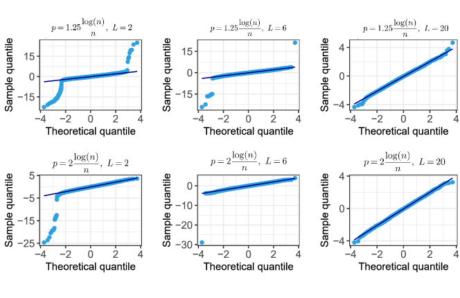
Figure 3: Q-Q Plots for Lagrangian debiased estimators, comparing quantiles of standardized Lagrangian debiased estimators with standard normal. We fix $n=100$ and let $L\in\{2,6,20\}$, $p\in\{1.25,2\}\times\frac{\log(n)}{n}$.

Next, we examine the performance of the pairwise test and top-$K$ test procedure in Section 3.2. For pairwise test, we test $H_{0}:\theta^{*}_{1}\leq\theta^{*}_{2}\text{\ \ v.s.\ \ }H_{a}:\theta^{*}_{1}>\theta^{*}_{2}$. Figure 4 (A) displays the Type I error with $p=0.2$ for different total number of items $n$ and number of repeated comparisons $L$. Here we fix $\theta^{*}_{1}=\theta^{*}_{2}=10$ and $\theta^{*}_{i}=7.5$ for $3\leq i\leq n$. As seen from this figure, the empirical Type I error rate is close to the nominal $\alpha=0.05$. Figure 4 (B) shows the empirical power of this test with different $\Delta=|\theta_{1}^{*}-\theta_{2}^{*}|$. Here we set $\theta^{*}_{1}=10,\theta^{*}_{2}=10-\Delta$ and $\theta^{*}_{i}=7.5$ for $3\leq i\leq n$, and we let $n=100$ and $p=0.2$ while change $\Delta$ and $L$. We observe that the empirical power goes to 1 quickly.

(A) Type I error	(B) Power

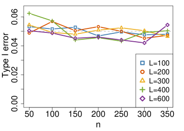
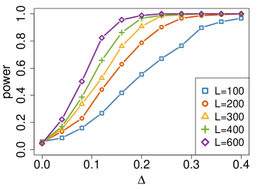
Figure 4: The performance of pairwise test $H_{0}:\theta^{*}_{1}\leq\theta^{*}_{2}\text{\ \ v.s.\ \ }H_{a}:\theta^{*}_{1}>\theta^{*}_{2}$. (A) Type I error for our proposed pairwise test procedure with different $n$ and $L$. (B) Power curve as a function of signal strength $\Delta=|\theta^{*}_{1}-\theta^{*}_{2}|$ with $n=100$, $p=0.2$ and $L\in\{100,200,300,400,600\}$.

For top-$K$ test, we test if item $K+1$ is ranked among the top $K$ items. We fix $K=30$ and $p=0.2$, and we let $\theta^{*}_{i}=10$ for $1\leq i\leq K+1$, and $\theta^{*}_{j}=7.5$ for $K+2\leq j\leq n$. Figure 5 (A) displays the empirical Type I error rate with different $n$ and $L$, and we find that that the empirical Type I error is close to the nominal $\alpha=0.05$. Figure 5 (B) displays the empirical power of this test with different separation $\Delta$ between top $K$ items and other items that $\Delta=|\theta^{*}_{(K)}-\theta^{*}_{(K+1)}|$. We let $n=100$, $L\in\{100,200,300,400,600\}$, and we set $\theta^{*}_{i}=10$ for $1\leq i\leq K$, $\theta^{*}_{K+1}=10-\Delta$, and $\theta^{*}_{j}=7.5$ for $K+2\leq j\leq n$. As seen from this plot, the empirical power goes to 1 as $\Delta$ and $L$ increase.

(A) Type I error	(B) Power

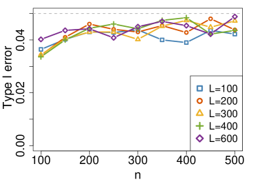
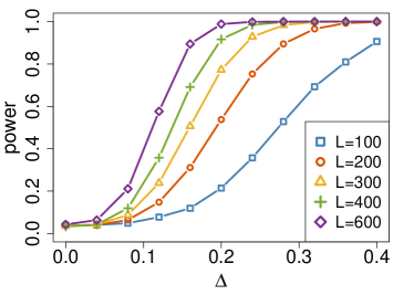
Figure 5: Performance of top-30 test using our proposed simplified testing procedure in Remark 3.15: (A) Averaged Type I error with different $n$ and $L$. (B) Averaged power as a function of signal strength $\Delta=|\theta^{*}_{(K)}-\theta^{*}_{(K+1)}|$ with $n=100$, $p=0.2$, and $L\in\{100,200,300,400,600\}$.

Finally, we evaluate the empirical performance of our FDR procedure in Section 4.2 by considering the top-$K$ test. We let $K=30$, $\theta^{*}_{i}=10$ for $1\leq i\leq K+10$, and $\theta^{*}_{j}=6.5$ for $K+11\leq j\leq n$. Figure 6 (A) displays the empirical FDR based on our procedure with $p=0.2$ and different $n$, $L$. This figure illustrates that the FDR is well controlled below the nominal $\alpha=0.05$, consistent with our results in Theorem 4.3. Figure 6 (B) displays the empirical power of the FDR procedure, which is defined as true positive rate, with different separation $\Delta=|\theta^{*}_{(K)}-\theta^{*}_{(K+1)}|$. We set $\theta^{*}_{i}=10$ for $1\leq i\leq K$, $\theta^{*}_{K+1}=10-\Delta$, and $\theta^{*}_{j}=6.5$ for $K+2\leq j\leq n$, and we let $n=100$, $p=0.2$, and $L\in\{100,200,300,400,600\}$. As shown in this plot, the empirical power increases and goes to 1 as $\Delta$ and $L$ increase, showing that the proposed FDR procedure is able to identify the top $K$ items with well controlled FDR.

(A) FDR	(B) FDR power

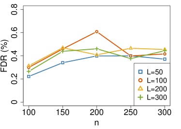
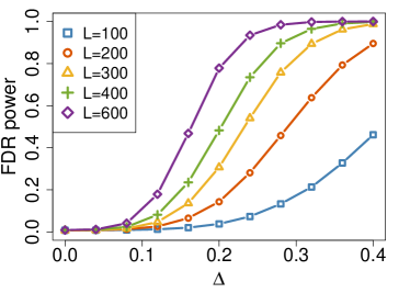
Figure 6: Performance of Benjamini-Yekutieli based FDR procedure for selecting top-30 items. (A) Empirical FDR with different $n$ and $L$. (B) Empirical FDR power as a function of signal strength $\Delta=|\theta_{(K)}-\theta_{(K+1)}|$ with $n=100$, $p=0.2$, and $L\in\{100,200,300,400,600\}$.

6.2 Real-World Data

In this section, We apply our method to analyze two real datasets.

Jester Dataset.

We first apply our method to the Jester dataset from Goldberg et al. (2001). This dataset contains ratings of 100 jokes from 73,421 users. The more detailed description and the dataset is available through http://eigentaste.berkeley.edu/dataset/. In this dataset, 14,116 users rated all 100 jokes, while others only rated some of jokes. We only use samples from users who ranked all 100 jokes for our experiments. Since we need pairwise comparisons for our ranking analysis, we generate Erdös-Rényi comparison graph randomly with $p=0.3$ and obtain each pairwise comparison results based on the relative rating of compared pairs by the same user. To be specific, if joke 1 receives a higher rating than joke 2 from a same user, we have joke 1 beats joke 2 in this comparison. Negahban et al. (2017), Kim et al. (2017) also use similar approaches to break rating results into pairwise comparisons. Further, we randomly choose $L$ samples from the total 14,116 samples.

Table 1 displays the top 10 jokes’ IDs and their estimated scores obtained from the spectral method and our debiasing method with $L=1000$. Furthermore, we evaluate the performance of our FDR-controlling procedure with $K\in\{20,40\}$ and $L\in\{1000,5000\}$. Figure 7 presents the p-values from multiple testing and threshold obtained from Benjamini-Yekutieli procedure described in Section 4.2. It shows that our FDR procedure gains more power as $L$ increases.

Table 1: The top 10 jokes on Jester Dataset and their estimated scores obtained from Spectral method and our Lagrangian debiasing method.

	Spectral method		Debiasing method
Joke ID	Score	Rank	Score	Rank
89	0.841	1	0.840	1
50	0.799	2	0.801	2
29	0.651	3	0.645	3
36	0.623	4	0.628	4
27	0.621	5	0.620	5
62	0.616	6	0.616	6
32	0.603	7	0.599	7
35	0.596	8	0.596	8
54	0.527	9	0.526	9
69	0.515	10	0.516	10

$(K=20,L=1000)$	$(K=40,L=1000)$
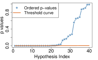
$(K=20,L=5000)$	$(K=40,L=5000)$

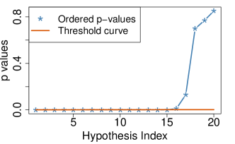
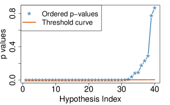
Figure 7: Application of our FDR procedure on Jester Dataset to select top $K$ jokes. The four panels display the ordered p-values and adjusted threshold by Benjamini-Yekutieli procedure with $K\in\{20,40\}$ and $L\in\{1000,5000\}$. The horizontal red line represents 0.05.

MovieLens Dataset

We also apply our method to analyze the MovieLens dataset (Harper and Konstan 2015). Similar to our analysis before, we obtain pairwise comparisons results based on the relative ratings of two movies by the same user. In particular, we analyze $n=218$ movies with largest number of ratings, and randomly sample $L=1000$ comparisons. Table 2 shows the top 10 movies with highest scores based on Lagrangian debiasing procedure and the corresponding p-values, where we test if they are ranked among the top 10 and top 20 movies. Figure 8 displays the change of p-values when each movie is tested if it is among top 1, 5, 10, 20 ranked movies. We display the p-values of four movies (The Shawshank Redemption, The Matrix, The Usual Suspects, Schindler’s List), which are ranked 1, 2, 5, 10 based on our debiased estimator.

Table 2: Top 10 movies in MovieLens Dataset based on Lagrangian debiased estimator. The table includes their titles, average rating in https://movielens.org/, estimated scores by Lagrangian debiased procedure, and their corresponding p-values in top 10 and top 20 test by our proposed testing procedure in Remark 3.15.

Rank	Movie Title	Average rating	Debiased Score	P-value in top 10 test	P-value in top 20 test
1	The Shawshank Redemption (1994)	4.42	1.985	$<1e-6$	$<1e-6$
2	The Matrix (1999)	4.16	1.766	$<1e-6$	$<1e-6$
3	The Godfather (1972)	4.25	1.755	$<1e-6$	$<1e-6$
4	Star Wars: Episode V - The Empire Strikes Back (1980)	4.12	1.684	$<1e-6$	$<1e-6$
5	The Usual Suspects (1995)	4.28	1.530	$<1e-6$	$<1e-6$
6	Star Wars: Episode IV - A New Hope (1977)	4.10	1.471	0.0010	$<1e-6$
7	The Silence of the Lambs (1991)	4.15	1.418	0.0070	$<1e-6$
8	Seven (a.k.a. Se7en) (1995)	4.08	1.367	0.0401	$<1e-6$
9	Lord of the Rings: The Fellowship of the Ring (2001)	4.10	1.329	0.1133	$<1e-6$
10	Schindler’s List (1993)	4.25	1.288	0.3431	0.0002

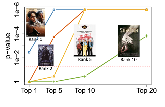
Figure 8: Application of top-$K$ test on four movies (The Shawshank Redemption, The Matrix, The Usual Suspects, Schindler’s List) in MovieLens Dataset, which are ranked 1, 2, 5, 10 based on Lagrangian debiasing estimator. The figure displays the change of their p-values in top 1, 5, 10, 20 test by our proposed testing procedure in Remark 3.15. The horizontal dotted red line represents 0.05

7 Conclusion

To conclude, to the best of our knowledge, we propose the first general framework for conducting inference and quantifying uncertainties for ranking problems. Under the BTL model, we first propose a Lagrangian debiasing method to infer the latent score for each item, where we can then test “local” properties. Next, by leveraging the powerfulness of Gaussian multiplier bootstrap, we can test more general “global” properties. Furthermore, we extend the framework to multiple testing problems where we control both the familywise Type I error and the false discovery rate. We prove the optimality of the proposed method by deriving the minimax lower bound. Using both synthetic and real datasets, we demonstrate that our method works well in practice.

There are still numerous promising directions that would be of interest for future investigations. We point out a few possibilities as follows. First, the Gaussian multiplier bootstrap approach is computationally expensive, and it is worth investigating if we can develop a more computationally efficient approach to make the method more scalable. Second, as we have discussed, the current approach for false discovery rate control is conservative, and we plan to develop a more powerful method to tightly control the false discovery rate. In addition, the ranking of different items may change over time, and we plan to develop new models to study dynamic ranking systems.

A Proof of Theorems in Section 3.1

A.1 Proof of Theorem 3.5

Proof A.1

We prove the asymptotic normality of the general Lagrangian debiasing estimator. First we decompose the general Lagrangian debiasing estimator as

$${\left(\begin{array}[]{ccc}\widehat{{\theta}}^{d}-{{\theta}}^{*}\\ \lambda\end{array}\right)}= {\ \left(\begin{array}[]{ccc}\widehat{{\theta}}^{d}-\widehat{{\theta}}\\ \lambda\end{array}\right)}+{\left(\begin{array}[]{ccc}\widehat{{\theta}}-{{\theta}}^{*}\\ 0\end{array}\right)}$$ (29)

$$= \ \widehat{\Theta}{\left(\begin{array}[]{ccc}-\nabla{\mathcal{L}({\widehat{{\theta}}})}\\ -f(\widehat{{\theta}})\end{array}\right)}+\widehat{\Theta}\widehat{\Sigma}{\left(\begin{array}[]{ccc}\widehat{{\theta}}-{{\theta}}^{*}\\ 0\end{array}\right)}+(I-\widehat{\Theta}\widehat{\Sigma}){\left(\begin{array}[]{ccc}\widehat{{\theta}}-{{\theta}}^{*}\\ 0\end{array}\right)}$$

$$= \ \widehat{\Theta}{\left(\begin{array}[]{ccc}-\nabla{\mathcal{L}({\widehat{{\theta}}})}\\ -f(\widehat{{\theta}})\end{array}\right)}+\widehat{\Theta}{\left(\begin{array}[]{ccc}\nabla^{2}\mathcal{L}(\widehat{{\theta}})(\widehat{{\theta}}-{\theta}^{*})\\ \nabla f(\widehat{{\theta}})^{\top}(\widehat{{\theta}}-{\theta}^{*})\end{array}\right)}+(I-\widehat{\Theta}\widehat{\Sigma}){\left(\begin{array}[]{ccc}\widehat{{\theta}}-{{\theta}}^{*}\\ 0\end{array}\right)}$$

$$= \ \widehat{\Theta}{\left(\begin{array}[]{ccc}-\nabla\mathcal{L}(\widehat{{\theta}})+\nabla^{2}\mathcal{L}(\widehat{{\theta}})(\widehat{{\theta}}-{\theta}^{*})\\ -f(\widehat{{\theta}})+\nabla f(\widehat{{\theta}})^{\top}(\widehat{{\theta}}-{\theta}^{*})\end{array}\right)}+(I-\widehat{\Theta}\widehat{\Sigma}){\left(\begin{array}[]{ccc}\widehat{{\theta}}-{{\theta}}^{*}\\ 0\end{array}\right)}$$

$$= \ {\Theta}^{*}{\left(\begin{array}[]{ccc}-\nabla\mathcal{L}({{\theta}}^{*})\\ -f({{\theta}}^{*})\end{array}\right)}+\underbrace{(\widehat{\Theta}-{\Theta}^{*})\left(\begin{array}[]{ccc}-\nabla\mathcal{L}(\widehat{{\theta}})+\nabla^{2}\mathcal{L}(\widehat{{\theta}})(\widehat{{\theta}}-{\theta}^{*})\\ -f(\widehat{{\theta}})+\nabla f(\widehat{{\theta}})^{\top}(\widehat{{\theta}}-{\theta}^{*})\end{array}\right)}_{J_{1}}$$

$$+\underbrace{{\Theta}^{*}\left(\begin{array}[]{ccc}\nabla\mathcal{L}({{\theta}}^{*})-\nabla\mathcal{L}(\widehat{{\theta}})+\nabla^{2}\mathcal{L}(\widehat{{\theta}})(\widehat{{\theta}}-{\theta}^{*})\\ f({{\theta}}^{*})-f(\widehat{{\theta}})+\nabla f(\widehat{{\theta}})^{\top}(\widehat{{\theta}}-{\theta}^{*})\end{array}\right)}_{J_{2}}+\underbrace{(I-\widehat{\Theta}\widehat{\Sigma})\left(\begin{array}[]{ccc}\widehat{{\theta}}-{{\theta}}^{*}\\ 0\end{array}\right)}_{J_{3}},$$

where the second equality comes from (9), the third equality comes from (7). Then we bound $J_{1}$, $J_{2}$ and $J_{3}$ in the following lemma, and the proof is provided in Section C.1.1.

Lemma A.2

Under the conditions of Theorem 3.5, we have

$$\|J_{1}\|_{\infty}\lesssim(r_{1}+r_{4})(r_{1}^{2}+r_{2}),$$ (30)

$$\|J_{2}\|_{\infty}\lesssim r_{1}^{2}r_{5},$$ (31)

$$\|J_{3}\|_{\infty}\lesssim r_{1}r_{3},$$ (32)

where $r_{1}$, $r_{2}$, $r_{3}$, $r_{4}$ and $r_{5}$ are defined in Assumptions 1 – 3.1.1.

Plugging (30), (31), (32) into (29), we have

$$\|J_{1}+J_{2}+J_{3}\|_{\infty}\lesssim r_{1}^{2}r_{5}+(r_{1}+r_{4})(r_{1}^{2}+r_{2})+r_{1}r_{3}.$$

Then, by our scaling assumption

$$\sqrt{n}(r_{1}^{2}r_{5}+(r_{1}+r_{4})(r_{1}^{2}+r_{2})+r_{1}r_{3})=o(1),$$

and Assumption 1, we immediately have

$$\sqrt{n}\frac{\widehat{{\theta}}_{j}^{d}-{{\theta}}^{*}_{j}}{\sqrt{[{\Theta}_{11}^{*}{\Sigma}^{*}_{11}{\Theta}_{11}^{*}]_{jj}}}=-\sqrt{n}\frac{[{\Theta}^{*}_{11}\nabla\mathcal{L}({{\theta}}^{*})]_{j}}{\sqrt{[{\Theta}_{11}^{*}{\Sigma}^{*}_{11}{\Theta}_{11}^{*}]_{jj}}}+o_{\mathchoice{\raisebox{-1.5pt}{$\displaystyle\mathbb{P}$}}{\raisebox{-1.5pt}{$\textstyle\mathbb{P}$}}{\raisebox{-1.5pt}{$\scriptstyle\mathbb{P}$}}{\raisebox{-1.5pt}{$\scriptscriptstyle\mathbb{P}$}}}(1)\overset{d}{\longrightarrow}N(0,1),$$

and

$$\sqrt{n}\frac{(\widehat{{\theta}}_{i}^{d}-{{\theta}}^{*}_{i})-(\widehat{{\theta}}_{j}^{d}-{{\theta}}^{*}_{j})}{\sqrt{(\bm{e}_{i}-\bm{e}_{j})^{\top}({\Theta}_{11}^{*}{\Sigma}^{*}_{11}{\Theta}_{11}^{*})(\bm{e}_{i}-\bm{e}_{j})}}=-\sqrt{n}\frac{[{\Theta}^{*}_{11}\nabla\mathcal{L}({\theta}^{*})]_{i}-[{\Theta}^{*}_{11}\nabla\mathcal{L}({\theta}^{*})]_{j}}{\sqrt{(\bm{e}_{i}-\bm{e}_{j})^{\top}({\Theta}_{11}^{*}{\Sigma}^{*}_{11}{\Theta}_{11}^{*})(\bm{e}_{i}-\bm{e}_{j})}}+{o_{\mathchoice{\raisebox{-1.5pt}{$\displaystyle\mathbb{P}$}}{\raisebox{-1.5pt}{$\textstyle\mathbb{P}$}}{\raisebox{-1.5pt}{$\scriptstyle\mathbb{P}$}}{\raisebox{-1.5pt}{$\scriptscriptstyle\mathbb{P}$}}}(1)}\overset{d}{\longrightarrow}N(0,1),$$

which concludes our proof.

A.2 Proof of Theorem 3.8

Proof A.3

First, by simple algebra, we have that the gradient and the Hessian of negative log likelihood function $\mathcal{L}({\theta})$ defined in (3) are

$$\nabla{\mathcal{L}({\theta})}=\sum_{i>j}{\mathcal{E}_{ji}}(-y_{ji}+\frac{e^{\theta_{i}}}{e^{\theta_{i}}+e^{\theta_{j}}})(\bm{e}_{i}-\bm{e}_{j}),$$ (33)

and

$$\nabla^{2}{\mathcal{L}({\theta})}=\sum_{i>j}{\mathcal{E}_{ji}}\frac{e^{\theta_{i}}e^{\theta_{j}}}{(e^{\theta_{i}}+e^{\theta_{j}})^{2}}(\bm{e}_{i}-\bm{e}_{j})(\bm{e}_{i}-\bm{e}_{j})^{\top}$$ (34)

where $\mathcal{E}_{ji}=1$ if $(i,j)\in\mathcal{E}$, $\mathcal{E}_{ji}=0$ otherwise, and $\mathcal{E}$ is the comparison graph.

Similar to the proof of Theorem 3.5, by simple algebra, $\widehat{{\theta}}^{d}-{\theta}^{*}$ can be decomposed as

$${\Bigg{(}\begin{array}[]{ccc}\widehat{{\theta}}^{d}-{\theta}^{*}\\ \lambda\end{array}\Bigg{)}}= \ \underbrace{\Bigg{(}{\Bigg{(}\begin{array}[]{ccc}\nabla^{2}{\mathcal{L}(\widehat{{\theta})}}&\bm{1}\\ \bm{1}^{\top}&0\end{array}\Bigg{)}}^{-1}-{\Bigg{(}\begin{array}[]{ccc}\nabla^{2}{\mathcal{L}({{\theta}}^{*})}&\bm{1}\\ \bm{1}^{\top}&0\end{array}\Bigg{)}}^{-1}\Bigg{)}{\Bigg{(}\begin{array}[]{ccc}-\nabla\mathcal{L}(\widehat{{\theta}})+\nabla^{2}\mathcal{L}(\widehat{{\theta}})(\widehat{{\theta}}-{\theta}^{*})\\ 0\end{array}\Bigg{)}}}_{I_{1}}$$ (35)

$$+\underbrace{\Bigg{(}\begin{array}[]{ccc}\nabla^{2}{\mathcal{L}({{\theta}^{*}})}&\bm{1}\\ \bm{1}^{\top}&0\end{array}\Bigg{)}^{-1}{\Bigg{(}\begin{array}[]{ccc}\nabla\mathcal{L}({{\theta}}^{*})-\nabla\mathcal{L}(\widehat{{\theta}})+\nabla^{2}\mathcal{L}(\widehat{{\theta}})(\widehat{{\theta}}-{\theta}^{*})\\ 0\end{array}\Bigg{)}}}_{I_{2}}$$

$$+{\Bigg{(}\begin{array}[]{ccc}\nabla^{2}{\mathcal{L}({{\theta}}^{*})}&\bm{1}\\ \bm{1}^{\top}&0\end{array}\Bigg{)}}^{-1}{\Bigg{(}\begin{array}[]{ccc}-\nabla\mathcal{L}({{\theta}}^{*})\\ 0\end{array}\Bigg{)}}.$$

Note that we have two parts of randomness here. The first part comes from the random comparison graph $\mathcal{E}$, and the other part comes from the binary pairwise comparison outcome $y_{i,j}^{(\ell)}$ in (1). In what follows, to obtain the asymptotic normality of the debiasing estimator, we first derive some bounds for the objective which depend on the randomness of $\mathcal{E}$, and then derive the conditional asymptotic distribution of $\widehat{{\theta}}^{d}-{\theta}^{*}$ by conditioning on the comparison graph $\mathcal{E}$ such that we only have randomness from the binary outcome $y_{i,j}^{(\ell)}$.

In particular, by the randomness of the graph $\mathcal{E}$, the next lemma derives some inequalities, which are essential for deriving the bounds for $I_{1}$ and $I_{2}$. We provide the proof in Section C.2.1.

Lemma A.4

Under the conditions of Theorem 3.8, we have that, with probability at least $1-\mathcal{O}(n^{-5})$,

$$\|{\nabla\mathcal{L}({{\theta}}^{*})}\|_{\infty}\lesssim np\sqrt{\frac{\log n}{L}},$$ (36)

$$\|\nabla\mathcal{L}(\widehat{{\theta}})-\nabla\mathcal{L}({{\theta}}^{*})-\nabla^{2}\mathcal{L}({\theta}^{*})(\widehat{{\theta}}-{\theta}^{*})\|_{\infty}\lesssim\frac{\log n}{L},$$ (37)

$$\|\nabla^{2}{\mathcal{L}(\widehat{{\theta})}}-\nabla^{2}{\mathcal{L}({{\theta}}^{*})}\|_{\infty}\lesssim np\sqrt{\frac{\log n}{npL}},$$ (38)

$$\left\|{\left(\begin{array}[]{ccc}\nabla^{2}{\mathcal{L}({{{\theta}})}}&\bm{1}\\ \bm{1}^{\top}&0\end{array}\right)^{-1}}\right\|_{2}=\frac{1}{\lambda_{n-1}\left(\nabla^{2}\mathcal{L}({{{\theta}}})\right)}\lesssim\frac{1}{np},$$ (39)

$$\left\|{\left(\begin{array}[]{ccc}\nabla^{2}{\mathcal{L}(\widehat{{\theta})}}&\bm{1}\\ \bm{1}^{\top}&0\end{array}\right)}^{-1}-{\left(\begin{array}[]{ccc}\nabla^{2}{\mathcal{L}({{\theta}}^{*})}&\bm{1}\\ \bm{1}^{\top}&0\end{array}\right)}^{-1}\right\|_{2}\lesssim\frac{1}{np}\sqrt{\frac{\log n}{pL}}.$$ (40)

The next lemma derives the upper bounds of the terms $I_{1}$ and $I_{2}$ conditioning on the graph $\mathcal{E}$ based on the above lemma. We provide the proof in Section C.2.2.

Lemma A.5

Under the BTL model, suppose that the conditions of Theorem 3.8 hold, and suppose that conditioning on the random graph $\mathcal{E}$, (36), (37), (38), (39), and (40) hold. We have that

$$\|I_{1}\|_{\infty}\lesssim\frac{\sqrt{n}\log n}{\sqrt{p}\ L},\quad\text{ and }\quad\|I_{2}\|_{\infty}\lesssim\frac{\log n}{\sqrt{n}pL}.$$

Meanwhile, by the fact that

$${\left(\begin{array}[]{ccc}{\Theta}^{*}_{11}&\frac{1}{n}\bm{1}\\ \frac{1}{n}\bm{1}^{\top}&0\end{array}\right)}={\left(\begin{array}[]{ccc}\nabla^{2}{\mathcal{L}({{\theta}^{*})}}&\bm{1}\\ \bm{1}^{\top}&0\end{array}\right)^{-1}},$$

we immediately have

$$\widehat{{\theta}}^{d}-{\theta}^{*}=-{\Theta}^{*}_{11}\nabla{\mathcal{L}({{\theta}^{*})}}+r,$$ (41)

where $\|r\|_{\infty}\leq\|I_{1}\|_{\infty}+\|I_{2}\|_{\infty}\lesssim\frac{\sqrt{n}\log n}{\sqrt{p}\ L}+\frac{\log n}{\sqrt{n}pL}$. By our assumption that $\frac{n\log n}{\sqrt{L}}+\frac{\log n}{\sqrt{pL}}=o(1)$, we have $\sqrt{npL}\|r\|_{\infty}=o(1)$.

To obtain the conditional asymptotic distribution of $\widehat{{\theta}}^{d}-{\theta}^{*}$, we have the following lemma about the asymptotic distribution of ${\Theta}^{*}_{11}\nabla{\mathcal{L}({{\theta}^{*})}}$ conditioning on graph $\mathcal{E}$, and the proof is provided in Section C.2.3.

Lemma A.6 (Central Limit Theorem)

Under BTL model, assume the conditions of Theorem 3.8 are satisfied. Suppose that the comparison graph $\mathcal{E}$ satisfies conditions (36), (37), (38), (39), (40). We have

$$\sqrt{L}\ \frac{[{\Theta_{11}^{*}}]_{j}\nabla\mathcal{L}(\bm{\theta}^{*})}{\sqrt{[{\Theta}^{*}_{11}]_{jj}}}\,\Big{|}\,\mathcal{E}\xrightarrow{d}N(0,1),$$

and

$$\sqrt{L}\frac{([{\Theta}^{*}_{11}]_{i}-[{\Theta}^{*}_{11}]_{j})\nabla\mathcal{L}(\bm{\theta}^{*})}{\sqrt{(\bm{e}_{i}-\bm{e}_{j})^{\top}{\Theta}^{*}_{11}(\bm{e}_{i}-\bm{e}_{j})}}\ \,\Big{|}\,\mathcal{E}\xrightarrow{d}N(0,1),$$

where $[{\Theta_{11}^{*}}]_{j}$ is the $j$-th row of matrix ${\Theta_{11}^{*}}$, and $[{\Theta_{11}^{*}}]_{jj}$ is the $j$-th diagonal element of ${\Theta_{11}^{*}}$.

Combining (41) with the above central limit theorem, conditioning on comparison graph $\mathcal{E}$, we have the following asymptotic distributions that

$$\sqrt{L}\ \dfrac{\widehat{\theta}^{d}_{j}-{\theta}_{j}^{*}}{\sqrt{[{\Theta}^{*}_{11}]_{jj}}}\,\Big{|}\,\mathcal{E}\xrightarrow{d}N(0,1),\quad\text{and}\quad\sqrt{L}\frac{{\widehat{\theta}^{d}}_{h}-{\widehat{\theta}^{d}}_{j}-({{\theta}}^{*}_{h}-{{\theta}}^{*}_{j})}{\sqrt{(\bm{e}_{h}-\bm{e}_{j})^{\top}({\Theta}^{*}_{11})(\bm{e}_{h}-\bm{e}_{j})}}\,\Big{|}\,\mathcal{E}\xrightarrow{d}N(0,1).$$

Meanwhile, by Lemma A.4, we have that the conditions (36), (37), (38), (39), (40) are satisfied with probability at least $1-\mathcal{O}(n^{-5})$, and our claim holds as desired.

B Proofs of Corollaries in Section 3.1.1

B.1 Proof of Corollary 3.3

Proof B.1

To prove $\big{\|}\widehat{\Theta}-\Theta^{*}\big{\|}_{\infty}\lesssim r_{1}+r_{4}$, recall that $\widehat{\Theta}=\Big{(}\begin{smallmatrix}\widehat{\Theta}_{11}&\widehat{\Theta}_{12}\\ \widehat{\Theta}_{12}^{\top}&\widehat{\Theta}_{22}\end{smallmatrix}\Big{)}$, where

$$\widehat{\Theta}_{11}=\widehat{\Omega}-\widehat{\Omega}\nabla{f(\widehat{{\theta}})}\big{(}\nabla{f(\widehat{{\theta}})}^{\top}\widehat{\Omega}\nabla{f(\widehat{{\theta}})}\big{)}^{-1}\nabla{f(\widehat{{\theta}})}^{\top}\widehat{\Omega},$$

$$\widehat{\Theta}_{12}=\widehat{\Omega}\nabla{f(\widehat{{\theta}})}\big{(}\nabla{f(\widehat{{\theta}})}^{\top}\widehat{\Omega}\nabla{f(\widehat{{\theta}})}\big{)}^{-1},\ \text{ and }\ \widehat{\Theta}_{22}=-\big{(}\nabla{f(\widehat{{\theta}})}^{\top}\widehat{\Omega}\nabla{f(\widehat{{\theta}})}\big{)}^{-1}.$$

Also recall that $r_{1},r_{2},r_{3},r_{4},r_{5}=o(1)$, and $L_{1},L_{2},c_{1},c_{2},c_{3}$ are constants defined in Assumptions 1 – 3.1.1. Before going further, we first have the following two inequalities what are used in bounding $\widehat{\Theta}-\Theta^{*}$,

$$\big{\|}\nabla{f(\widehat{{\theta}})}^{\top}\widehat{\Omega}-\nabla{f({{\theta}}^{*})}^{\top}\Omega^{*}\big{\|}_{\infty}= \ \big{\|}\nabla{f(\widehat{{\theta}})}^{\top}(\widehat{\Omega}-\Omega^{*})+(\nabla{f(\widehat{{\theta}})}^{\top}-\nabla{f({{\theta}}^{*})}^{\top})\Omega^{*}\big{\|}_{\infty}$$

$$\lesssim \ (c_{1}+L_{2}r_{1})r_{4}+L_{2}r_{1}c_{2}\lesssim r_{1}+r_{4},$$

and

$$\big{|}\nabla{f(\widehat{{\theta}})}^{\top}\widehat{\Omega}\nabla{f(\widehat{{\theta}})}-\nabla{f({{\theta}}^{*})}^{\top}\Omega^{*}\nabla{f({{\theta}}^{*})}\big{|}$$

$$\quad=\big{|}\big{(}\nabla{f(\widehat{{\theta}})}^{\top}\widehat{\Omega}-\nabla{f({{\theta}}^{*})}^{\top}\Omega^{*}\big{)}\nabla{f(\widehat{{\theta}})}+\nabla{f({{\theta}}^{*})}^{\top}\Omega^{*}(\nabla f(\widehat{{\theta}})-\nabla f({{\theta}}^{*}))\big{|}$$

$$\quad\leq\big{\|}\nabla{f(\widehat{{\theta}})}^{\top}\widehat{\Omega}-\nabla{f({{\theta}}^{*})}^{\top}\Omega^{*}\big{\|}_{\infty}\big{\|}\nabla{f(\widehat{{\theta}})}\big{\|}_{\infty}+\big{\|}\nabla{f({{\theta}}^{*})}\big{\|}_{\infty}\big{\|}\Omega^{*}\big{\|}_{\infty}\big{\|}\nabla f(\widehat{{\theta}})-\nabla f({{\theta}}^{*})\big{\|}_{\infty}$$

$$\quad\lesssim(r_{1}+r_{4})(L_{2}r_{1}+c_{1})+c_{1}c_{2}L_{2}r_{1}\lesssim r_{1}+r_{4}.$$

Then, we bound each block of $\widehat{\Theta}-\Theta^{*}$ separately. We first have

$$\big{|}\widehat{\Theta}_{22}-\Theta^{*}_{22}\big{|}= \ \big{|}\big{(}\nabla{f(\widehat{{\theta}})}^{\top}\widehat{\Omega}\nabla{f(\widehat{{\theta}})}\big{)}^{-1}-\big{(}\nabla{f({{\theta}}^{*})}^{\top}\Omega^{*}\nabla{f({{\theta}}^{*})}\big{)}^{-1}\big{|}$$ (42)

$$\leq \ \big{|}\big{(}\nabla{f(\widehat{{\theta}})}^{\top}\widehat{\Omega}\nabla{f(\widehat{{\theta}})}\big{)}^{-1}\big{|}\big{|}\nabla{f(\widehat{{\theta}})}^{\top}\widehat{\Omega}\nabla{f(\widehat{{\theta}})}$$

$$\ -\nabla{f({{\theta}}^{*})}^{\top}\Omega^{*}\nabla{f({{\theta}}^{*})}\big{|}\big{|}\big{(}\nabla{f({{\theta}}^{*})}^{\top}\Omega^{*}\nabla{f({{\theta}}^{*})}\big{)}^{-1}\big{|}$$

$$\lesssim \ \frac{r_{1}+r_{4}}{(c_{3}-(r_{1}+r_{4}))c_{3}}\lesssim r_{1}+r_{4},$$

where the second inequality holds since

$$\big{|}\nabla{f(\widehat{{\theta}})}^{\top}\widehat{\Omega}\nabla{f(\widehat{{\theta}})}\big{|}\geq\big{|}\nabla{f({{\theta}}^{*})}^{\top}\Omega^{*}\nabla{f({{\theta}}^{*})}\big{|}-\big{|}\nabla{f(\widehat{{\theta}})}^{\top}\widehat{\Omega}\nabla{f(\widehat{{\theta}})}-\nabla{f({{\theta}}^{*})}^{\top}\Omega^{*}\nabla{f({{\theta}}^{*})}\big{|}\gtrsim c_{3}-(r_{1}+r_{4}),$$

and the last inequality holds since $r_{1},r_{4}=o(1)$ and $c_{3}=\mathcal{O}(1)$ by assumptions. Next, we have

$$\big{\|}\widehat{\Theta}_{12}-\Theta^{*}_{12}\big{\|}_{\infty}= \ \big{\|}\widehat{\Omega}\nabla{f(\widehat{{\theta}})}\big{(}\nabla{f(\widehat{{\theta}})}^{\top}\widehat{\Omega}\nabla{f(\widehat{{\theta}})}\big{)}^{-1}-\Omega^{*}\nabla{f({{\theta}}^{*})}\big{(}\nabla{f({{\theta}}^{*})}^{\top}\Omega^{*}\nabla{f({{\theta}}^{*})}\big{)}^{-1}\|_{\infty}$$ (43)

$$\leq \ \big{\|}\widehat{\Omega}\nabla{f(\widehat{{\theta}})}\|_{\infty}\big{|}\big{(}\nabla{f(\widehat{{\theta}})}^{\top}\widehat{\Omega}\nabla{f(\widehat{{\theta}})}\big{)}^{-1}-\big{(}\nabla{f({{\theta}}^{*})}^{\top}\Omega^{*}\nabla{f({{\theta}}^{*})}\big{)}^{-1}\big{|}$$

$$+\big{\|}\widehat{\Omega}\nabla{f(\widehat{{\theta}})}-\Omega^{*}\nabla{f({{\theta}}^{*})}\|_{\infty}\big{|}\big{(}\nabla{f({{\theta}}^{*})}^{\top}\Omega^{*}\nabla{f({{\theta}}^{*})}\big{)}^{-1}\big{|}$$

$$\lesssim \ (r_{1}+r_{4}+c_{2}c_{1})(r_{1}+r_{4})+\frac{(r_{1}+r_{4})}{c_{3}}\lesssim r_{1}+r_{4},$$

where the last ineuality holds since $\big{\|}\widehat{\Omega}\nabla{f(\widehat{{\theta}})}\|_{\infty}\leq\big{\|}\nabla{f({{\theta}}^{*})}^{\top}\Omega^{*}\big{\|}_{\infty}+\big{\|}\nabla{f(\widehat{{\theta}})}^{\top}\widehat{\Omega}-\nabla{f({{\theta}}^{*})}^{\top}\Omega^{*}\big{\|}_{\infty}\lesssim c_{1}c_{2}+r_{4}+r_{1}.$ Similarly, we have

$$\big{\|}\widehat{\Theta}_{11}-\Theta^{*}_{11}\big{\|}_{\infty}= \ \big{\|}\widehat{\Omega}-\widehat{\Omega}\nabla{f(\widehat{{\theta}})}\big{(}\nabla{f(\widehat{{\theta}})}^{\top}\widehat{\Omega}\nabla{f(\widehat{{\theta}})}\big{)}^{-1}\nabla{f(\widehat{{\theta}})}^{\top}\widehat{\Omega}-\Omega^{*}$$ (44)

$$+\Omega^{*}\nabla{f({{\theta}}^{*})}\big{(}\nabla{f({{\theta}}^{*})}^{\top}\Omega^{*}\nabla{f({{\theta}}^{*})}\big{)}^{-1}\nabla{f({{\theta}}^{*})}^{\top}\Omega^{*}\|_{\infty}$$

$$\leq \ \big{\|}\widehat{\Omega}-\Omega^{*}\|_{\infty}+\big{\|}\widehat{\Theta}_{12}-\Theta^{*}_{12}\big{\|}_{\infty}\big{\|}\nabla{f(\widehat{{\theta}})}^{\top}\widehat{\Omega}\big{\|}_{\infty}$$

$$+\big{\|}\Omega^{*}\nabla{f({{\theta}}^{*})}\big{(}\nabla{f({{\theta}}^{*})}^{\top}\Omega^{*}\nabla{f({{\theta}}^{*})}\big{)}^{-1}\big{\|}_{\infty}\big{\|}\nabla{f(\widehat{{\theta}})}^{\top}\widehat{\Omega}-\nabla{f({{\theta}}^{*})}^{\top}\Omega^{*}\big{\|}_{\infty}$$

$$\lesssim \ r_{4}+(r_{1}+r_{4})(r_{1}+r_{4}+c_{1}c_{2})+(r_{1}+r_{4})(r_{1}+r_{4})\lesssim r_{1}+r_{4}.$$

Combining (42), (43), (44) together, we have that $\big{\|}\widehat{\Theta}-\Theta^{*}\big{\|}_{\infty}\lesssim r_{1}+r_{4}$, which completes the proof.

B.2 Proof of Corollary 3.4

Proof B.2

To prove $\|I-\widehat{\Theta}\widehat{\Sigma}\|_{\infty}\lesssim r_{3}$, recall that $\widehat{\Sigma}=\Big{(}\begin{smallmatrix}\nabla^{2}{\mathcal{L}(\widehat{{\theta}})}&\nabla{f(\widehat{{\theta}})}\\ \nabla{f(\widehat{{\theta}})}^{\top}&0\end{smallmatrix}\Big{)}$, $r_{1},r_{2},r_{3},r_{4},r_{5}=o(1)$, and $L_{1},L_{2},c_{1},c_{2},c_{3}$ are constants defined in Assumptions 1 – 3.1.1. We bound the four blocks in $I-\widehat{\Theta}\widehat{\Sigma}$ separately. First, we have

$$\big{\|}(I-\widehat{\Theta}\widehat{\Sigma})_{11}\big{\|}_{\infty}= \ \Big{\|}\big{(}I-\widehat{\Omega}\nabla{f(\widehat{{\theta}})}\big{(}\nabla{f(\widehat{{\theta}})}^{\top}\widehat{\Omega}\nabla{f(\widehat{{\theta}})}\big{)}^{-1}\nabla{f(\widehat{{\theta}})}^{\top}\big{)}\big{(}\widehat{\Omega}\nabla^{2}{\mathcal{L}(\widehat{{\theta}})}-I\big{)}\Big{\|}_{\infty}$$

$$\leq \ \Big{\|}I-\widehat{\Omega}\nabla{f(\widehat{{\theta}})}\big{(}\nabla{f(\widehat{{\theta}})}^{\top}\widehat{\Omega}\nabla{f(\widehat{{\theta}})}\big{)}^{-1}\nabla{f(\widehat{{\theta}})}^{\top}\Big{\|}_{\infty}\big{\|}\widehat{\Omega}\nabla^{2}{\mathcal{L}(\widehat{{\theta}})}-I\big{\|}_{\infty},$$

where

$$\Big{\|}I-\widehat{\Omega}\nabla{f(\widehat{{\theta}})}\big{(}\nabla{f(\widehat{{\theta}})}^{\top}\widehat{\Omega}\nabla{f(\widehat{{\theta}})}\big{)}^{-1}\nabla{f(\widehat{{\theta}})}^{\top}\Big{\|}_{\infty}$$

$$\quad\leq\Big{\|}I-\Omega^{*}\nabla{f({{\theta}}^{*})}\big{(}\nabla{f({{\theta}}^{*})}^{\top}\Omega^{*}\nabla{f({{\theta}}^{*})}\big{)}^{-1}\nabla{f({{\theta}}^{*})}^{\top}\Big{\|}_{\infty}$$

$$\qquad+\Big{\|}\Omega^{*}\nabla{f({{\theta}}^{*})}\big{(}\nabla{f({{\theta}}^{*})}^{\top}\Omega^{*}\nabla{f({{\theta}}^{*})}\big{)}^{-1}\nabla{f({{\theta}}^{*})}^{\top}-\widehat{\Omega}\nabla{f(\widehat{{\theta}})}\big{(}\nabla{f(\widehat{{\theta}})}^{\top}\widehat{\Omega}\nabla{f(\widehat{{\theta}})}\big{)}^{-1}\nabla{f(\widehat{{\theta}})}^{\top}\Big{\|}_{\infty}$$

$$\quad\leq\Big{\|}I-\Omega^{*}\nabla{f({{\theta}}^{*})}\big{(}\nabla{f({{\theta}}^{*})}^{\top}\Omega^{*}\nabla{f({{\theta}}^{*})}\big{)}^{-1}\nabla{f({{\theta}}^{*})}^{\top}\Big{\|}_{\infty}+\big{\|}\widehat{\Theta}_{12}-\Theta^{*}_{12}\big{\|}_{\infty}\big{\|}\nabla{f(\widehat{{\theta}})}\big{\|}_{\infty}$$

$$\qquad+\Big{\|}\Omega^{*}\nabla{f({{\theta}}^{*})}\big{(}\nabla{f({{\theta}}^{*})}^{\top}\Omega^{*}\nabla{f({{\theta}}^{*})}\big{)}^{-1}\Big{\|}_{\infty}\big{\|}\nabla{f(\widehat{{\theta}})}-\nabla{f({{\theta}^{*}})}\big{\|}_{\infty}$$

$$\quad\lesssim(1+c_{2}c_{1}^{2}/c_{3})+(r_{1}+r_{4})(c_{1}+L_{2}r_{1})+(c_{2}c_{1}/c_{3})(L_{2}r_{1})\lesssim 1,$$

where we used the fact that

$$\widehat{\Theta}_{12}-\Theta^{*}_{12}=\widehat{\Omega}\nabla{f(\widehat{{\theta}})}\big{(}\nabla{f(\widehat{{\theta}})}^{\top}\widehat{\Omega}\nabla{f(\widehat{{\theta}})}\big{)}^{-1}-\Omega^{*}\nabla{f({{\theta}}^{*})}\big{(}\nabla{f({{\theta}}^{*})}^{\top}\Omega^{*}\nabla{f({{\theta}}^{*})}\big{)}^{-1}.$$

Thus,

$$\big{\|}(I-\widehat{\Theta}\widehat{\Sigma})_{11}\big{\|}_{\infty}\lesssim r_{3}.$$

Similarly, we have

$$\|(I-\widehat{\Theta}\widehat{\Sigma})_{21}\|_{\infty}= \ \Big{\|}\big{(}\nabla{f(\widehat{{\theta}})}^{\top}\widehat{\Omega}\nabla{f(\widehat{{\theta}})}\big{)}^{-1}\nabla{f(\widehat{{\theta}})}^{\top}\big{(}\widehat{\Omega}\nabla^{2}{\mathcal{L}(\widehat{{\theta}})}^{\top}-I\big{)}\Big{\|}_{\infty}$$

$$\leq \ \Big{\|}\big{(}\nabla{f(\widehat{{\theta}})}^{\top}\widehat{\Omega}\nabla{f(\widehat{{\theta}})}\big{)}^{-1}\nabla{f(\widehat{{\theta}})}^{\top}\Big{\|}_{\infty}\Big{\|}\widehat{\Omega}\nabla^{2}{\mathcal{L}(\widehat{{\theta}})}^{\top}-I\Big{\|}_{\infty}$$

$$\leq \ \Big{\{}\Big{\|}\big{(}\nabla{f({{\theta}}^{*})}^{\top}\Omega^{*}\nabla{f({{\theta}}^{*})}\big{)}^{-1}\nabla{f(\widehat{{\theta}})}^{\top}\Big{\|}_{\infty}+\big{|}\widehat{\Theta}_{22}-\Theta^{*}_{22}\big{|}\big{\|}\nabla{f(\widehat{{\theta}})}\big{\|}_{\infty}\Big{\}}\big{\|}\widehat{\Omega}\nabla^{2}{\mathcal{L}(\widehat{{\theta}})}^{\top}-I\big{\|}_{\infty}$$

$$\lesssim \ \Big{\{}(c_{1}+L_{2}r_{1})/c_{3}+(r_{1}+r_{4})(c_{1}+L_{2}r_{1})\Big{\}}r_{3}\lesssim r_{3}.$$

Combining the above two inequalities with the fact that $(I-\widehat{\Theta}\widehat{\Sigma})_{22}=0$ by simple algebra, we conclude that $\|I-\widehat{\Theta}\widehat{\Sigma}\|_{\infty}\lesssim r_{3}.$

C Proofs of Lemmas in Section A

C.1 Proofs of Auxiliary Lemmas in Section A.1

C.1.1 Proof of Lemma A.2

Proof C.1

We bound $J_{1}$, $J_{2}$, and $J_{3}$ separately. Recall that $r_{1},r_{2},r_{3},r_{4},r_{5}=o(1)$, and $L_{1},L_{2},c_{1},c_{2},c_{3}$ are constants defined in Assumptions 1 – 3.1.1. To bound $J_{2}$, by Assumptions 1 and 1, we have

$$\|\nabla\mathcal{L}({{\theta}}^{*})-\nabla\mathcal{L}(\widehat{{\theta}})+\nabla^{2}\mathcal{L}(\widehat{{\theta}})(\widehat{{\theta}}-{\theta}^{*})\|_{\infty}$$

$$\quad\leq\|\nabla\mathcal{L}(\widehat{{\theta}})-\nabla\mathcal{L}({{\theta}}^{*})-\nabla^{2}\mathcal{L}({{\theta}}^{*})(\widehat{{\theta}}-{\theta}^{*})\|_{\infty}+\|\nabla^{2}\mathcal{L}(\widehat{{\theta}})-\nabla^{2}\mathcal{L}({{\theta}}^{*})\|_{\infty}\|\widehat{{\theta}}-{\theta}^{*}\|_{\infty}$$

$$\quad\lesssim\Big{\|}\int_{0}^{1}\Big{(}\nabla^{2}\mathcal{L}\big{(}{\theta}^{*}+t(\widehat{{\theta}}-{\theta}^{*})\big{)}-\nabla^{2}\mathcal{L}({{\theta}}^{*})\Big{)}\mathrm{d}t\ (\widehat{{\theta}}-{\theta}^{*})\Big{\|}_{\infty}+\|\nabla^{2}\mathcal{L}(\widehat{{\theta}})-\nabla^{2}\mathcal{L}({{\theta}}^{*})\|_{\infty}\|\widehat{{\theta}}-{\theta}^{*}\|_{\infty}$$

$$\quad\lesssim L_{1}\|\widehat{{\theta}}-{\theta}^{*}\|_{\infty}^{2}\lesssim L_{1}r_{1}^{2}.$$

Similarly, one can derive the same rate for $\|f({{\theta}}^{*})-f(\widehat{{\theta}})+\nabla f(\widehat{{\theta}})^{\top}(\widehat{{\theta}}-{\theta}^{*})\|_{\infty}\lesssim L_{2}r_{1}^{2}$, and we thus have a bound for $J_{2}$ that

$$\|J_{2}\|_{\infty}=\|{\Theta}^{*}\|_{\infty}\Bigg{\|}{\left(\begin{array}[]{ccc}\nabla\mathcal{L}({{\theta}}^{*})-\nabla\mathcal{L}(\widehat{{\theta}})+\nabla^{2}\mathcal{L}(\widehat{{\theta}})(\widehat{{\theta}}-{\theta}^{*})\\ f({{\theta}}^{*})-f(\widehat{{\theta}})+\nabla f(\widehat{{\theta}})^{\top}(\widehat{{\theta}}-{\theta}^{*})\end{array}\right)}\Bigg{\|}_{\infty}\lesssim r_{1}^{2}r_{5}.$$

Then we bound $J_{1}$. We first have, by Assumptions 1 and 1,

$$\|-\nabla\mathcal{L}(\widehat{{\theta}})+\nabla^{2}\mathcal{L}(\widehat{{\theta}})(\widehat{{\theta}}-{\theta}^{*})\|_{\infty}\lesssim\|\nabla\mathcal{L}({{\theta}}^{*})-\nabla\mathcal{L}(\widehat{{\theta}})+\nabla^{2}\mathcal{L}(\widehat{{\theta}})(\widehat{{\theta}}-{\theta}^{*})\|_{\infty}+\|\nabla\mathcal{L}({{\theta}}^{*})\|_{\infty}\lesssim L_{1}r_{1}^{2}+r_{2}.$$

Similarly, we have, by Assumptions 1 and 1,

$$\|-f(\widehat{{\theta}})+\nabla f(\widehat{{\theta}})^{\top}(\widehat{{\theta}}-{\theta}^{*})\|_{\infty}=\|f({{\theta}}^{*})-f(\widehat{{\theta}})+\nabla f(\widehat{{\theta}})^{\top}(\widehat{{\theta}}-{\theta}^{*})\|_{\infty}\lesssim L_{2}r_{1}^{2}.$$

Then, we have that

$$\|J_{1}\|_{\infty}\lesssim\|\widehat{\Theta}-{\Theta}^{*}\|_{\infty}\Bigg{\|}{\left(\begin{array}[]{ccc}-\nabla\mathcal{L}(\widehat{{\theta}})+\nabla^{2}\mathcal{L}(\widehat{{\theta}})(\widehat{{\theta}}-{\theta}^{*})\\ -f(\widehat{{\theta}})+\nabla f(\widehat{{\theta}})^{\top}(\widehat{{\theta}}-{\theta}^{*})\end{array}\right)}\Bigg{\|}_{\infty}\lesssim(r_{1}+r_{4})(r_{1}^{2}+r_{2}),$$

where we use the fact that $\big{\|}\widehat{\Theta}-\Theta^{*}\big{\|}_{\infty}\lesssim r_{1}+r_{4}$ from Corollary 3.3. Finally, we bound $J_{3}$ by Assumption 1 and Corollary 3.4 that

$$\|J_{3}\|_{\infty}=\|I-\widehat{\Theta}\widehat{\Sigma}\|_{\infty}\|\widehat{{\theta}}-{{\theta}}^{*}\|_{\infty}\lesssim r_{1}r_{3}.$$

Combining the three bounds, we conclude the proof.

C.2 Proofs of Auxiliary Lemmas in Section A.2

C.2.1 Proof of Lemma A.4

Proof C.2

In Lemmas C.3, C.5, C.7, C.9, C.11, we show that conditions (36), (37), (38), (39), (40) are satisfied with probability at least $1-\mathcal{O}(n^{-5})$. The proofs of these five lemmas can be found in Section H.

Lemma C.3 (Gradient concentration)

Under the conditions of Theorem 3.8, we have

$$\|{\nabla\mathcal{L}({{\theta}}^{*})}\|_{\infty}\lesssim np\sqrt{\frac{\log n}{L}}$$

with probability at least $1-\mathcal{O}(n^{-6}).$

Proof C.4

See Section H.2 for the detailed proof.

Lemma C.5 (Local smoothness condition)

Under the conditions of Theorem 3.8, we have

$$\|\nabla\mathcal{L}(\widehat{{\theta}})-\nabla\mathcal{L}({{\theta}}^{*})-\nabla^{2}\mathcal{L}({\theta}^{*})(\widehat{{\theta}}-{\theta}^{*})\|_{\infty}\lesssim\frac{\log n}{L}$$

with probability at least $1-\mathcal{O}(n^{-5})$.

Proof C.6

See Section H.3 for the detailed proof.

Lemma C.7 (Hessian concentration)

Under the conditions of Theorem 3.8, we have

$$\|\nabla^{2}{\mathcal{L}(\widehat{{\theta})}}-\nabla^{2}{\mathcal{L}({{\theta}}^{*})}\|_{\infty}\lesssim np\sqrt{\frac{\log n}{npL}}$$

with probability at least $1-\mathcal{O}(n^{-5})$.

Proof C.8

See Section H.4 for the detailed proof.

Lemma C.9

Under the conditions of Theorem 3.8, we have

$$\left\|{\left(\begin{array}[]{ccc}\nabla^{2}{\mathcal{L}({{{\theta}})}}&\bm{1}\\ \bm{1}^{\top}&0\end{array}\right)^{-1}}\right\|_{2}=\frac{1}{\lambda_{n-1}\left(\nabla^{2}\mathcal{L}({{{\theta}}})\right)}\lesssim\frac{1}{np}$$

with probability exceeding $1-\mathcal{O}(n^{-10})$, where ${\theta}$ can be either $\widehat{{\theta}}$ or ${\theta}^{*}$.

Proof C.10

See Section H.5 for the detailed proof.

Lemma C.11

Under the conditions of Theorem 3.8, we have

$$\left\|{\left(\begin{array}[]{ccc}\nabla^{2}{\mathcal{L}(\widehat{{\theta})}}&\bm{1}\\ \bm{1}^{\top}&0\end{array}\right)}^{-1}-{\left(\begin{array}[]{ccc}\nabla^{2}{\mathcal{L}({{\theta}}^{*})}&\bm{1}\\ \bm{1}^{\top}&0\end{array}\right)}^{-1}\right\|_{2}\lesssim\frac{1}{np}\sqrt{\frac{\log n}{pL}}$$

with probability at least $1-\mathcal{O}(n^{-5})$.

Proof C.12

See Section H.6 for the detailed proof.

C.2.2 Proof of Lemma A.5

Proof C.13

We bound $I_{1}$ and $I_{2}$ in (35) based on (36), (37), (38), (39), and (40). First, we have that

$$\|I_{1}\|_{\infty}\leq \ \left\|{\left(\begin{array}[]{ccc}\nabla^{2}{\mathcal{L}(\widehat{{\theta})}}&\bm{1}\\ \bm{1}^{\top}&0\end{array}\right)}^{-1}-{\left(\begin{array}[]{ccc}\nabla^{2}{\mathcal{L}({{\theta}}^{*})}&\bm{1}\\ \bm{1}^{\top}&0\end{array}\right)}^{-1}\right\|_{\infty}\cdot\left\|{-\nabla\mathcal{L}(\widehat{{\theta}})+\nabla^{2}\mathcal{L}({\theta}^{*})(\widehat{{\theta}}-{\theta}^{*})}\right\|_{\infty}$$ (45)

$$\lesssim \ \sqrt{n+1}\left\|{\left(\begin{array}[]{ccc}\nabla^{2}{\mathcal{L}(\widehat{{\theta})}}&\bm{1}\\ \bm{1}^{\top}&0\end{array}\right)}^{-1}-{\left(\begin{array}[]{ccc}\nabla^{2}{\mathcal{L}({{\theta}}^{*})}&\bm{1}\\ \bm{1}^{\top}&0\end{array}\right)}^{-1}\right\|_{2}\left\|{-\nabla\mathcal{L}(\widehat{{\theta}})+\nabla^{2}\mathcal{L}({\theta}^{*})(\widehat{{\theta}}-{\theta}^{*})}\right\|_{\infty}$$

$$\lesssim \ \sqrt{n+1}\cdot\frac{1}{np}\sqrt{\frac{\log n}{pL}}\cdot\left(np\sqrt{\frac{\log n}{L}}+\frac{\log n}{L}\right)\lesssim\frac{\sqrt{n}\log n}{\sqrt{p}\ L},$$

where the third inequality follows from (40) and the fact $\left\|{-\nabla\mathcal{L}(\widehat{{\theta}})+\nabla^{2}\mathcal{L}({\theta}^{*})(\widehat{{\theta}}-{\theta}^{*})}\right\|_{\infty}\leq\big{\|}{\nabla\mathcal{L}({{\theta}}^{*})}\big{\|}_{\infty}+\big{\|}\nabla\mathcal{L}(\widehat{{\theta}})-\nabla\mathcal{L}({\theta}^{*})-\nabla^{2}\mathcal{L}({\theta}^{*})(\widehat{{\theta}}-{\theta}^{*})\big{\|}_{\infty}\lesssim np\sqrt{\frac{\log n}{L}}+\frac{\log n}{L}$ by (36) and (37), and the last inequality follows from the assumption that $p\gtrsim\frac{\log n}{n}$.

Next, we have that for the term $I_{2}$, by (37), (38) and (39),

$$\|I_{2}\|_{\infty} =\Bigg{\|}{\left(\begin{array}[]{ccc}\nabla^{2}{\mathcal{L}({{\theta}^{*}})}&\bm{1}\\ \bm{1}^{\top}&0\end{array}\right)}^{-1}{\left(\begin{array}[]{ccc}\nabla\mathcal{L}({{\theta}}^{*})-\nabla\mathcal{L}(\widehat{{\theta}})+\nabla^{2}\mathcal{L}(\widehat{{\theta}})(\widehat{{\theta}}-{\theta}^{*})\\ 0\end{array}\right)}\Bigg{\|}_{\infty}$$ (46)

$$\leq\sqrt{n+1}\left\|{\left(\begin{array}[]{ccc}\nabla^{2}{\mathcal{L}({{\theta}}^{*})}&\bm{1}\\ \bm{1}^{\top}&0\end{array}\right)}^{-1}\right\|_{2}\big{\|}\nabla\mathcal{L}({{\theta}}^{*})-\nabla\mathcal{L}(\widehat{{\theta}})+\nabla^{2}\mathcal{L}(\widehat{{\theta}})(\widehat{{\theta}}-{\theta}^{*})\big{\|}_{\infty}$$

$$\lesssim\sqrt{n+1}\times\frac{1}{np}\times\frac{\log n}{L}\lesssim\frac{\log n}{\sqrt{n}pL},$$

where the second inequality follows from $\big{\|}\nabla\mathcal{L}({{\theta}}^{*})-\nabla\mathcal{L}(\widehat{{\theta}})+\nabla^{2}\mathcal{L}(\widehat{{\theta}})(\widehat{{\theta}}-{\theta}^{*})\big{\|}_{\infty}\leq\big{\|}\nabla\mathcal{L}({{\theta}}^{*})-\nabla\mathcal{L}(\widehat{{\theta}})+\nabla^{2}\mathcal{L}({{\theta}^{*}})(\widehat{{\theta}}-{\theta}^{*})\big{\|}_{\infty}+\big{\|}(\nabla^{2}\mathcal{L}(\widehat{{\theta}})-\nabla^{2}\mathcal{L}({{\theta}^{*}}))(\widehat{{\theta}}-{\theta}^{*})\big{\|}_{\infty}\lesssim\frac{\log n}{L}+np\sqrt{\frac{\log n}{npL}}\times\sqrt{\frac{\log n}{npL}}\lesssim\frac{\log n}{L}$ by (37), (38) and Lemma 3.1. Combining (45) and (46), we complete the proof.

C.2.3 Proof of Lemma A.6

Proof C.14

To derive the conditional asymptotic normality, first, by the closed-form of gradient in (33), we decompose $[{\Theta}^{*}_{11}]_{j}\nabla\mathcal{L}({\theta}^{*})$ as a summation of independent random variables that

$$\left[\Theta^{*}_{11}\right]_{j}\nabla\mathcal{L}({\theta}^{*}) =\frac{1}{L}[{\Theta}^{*}_{11}]_{j}\sum_{\ell=1}^{L}\sum_{k>m,(k,m)\in\mathcal{E}}(-y_{m,k}^{(\ell)}+\frac{e^{\theta_{k}^{*}}}{e^{\theta_{k}^{*}}+e^{\theta_{m}^{*}}})(\bm{e}_{k}-\bm{e}_{m})$$

$$=\frac{1}{L}\sum_{\ell=1}^{L}\sum_{k>m,(k,m)\in\mathcal{E}}x_{m,k}^{(\ell)},$$

where $x_{m,k}^{(\ell)}:=[{\Theta}^{*}_{11}]_{j}\big{(}-y_{m,k}^{(\ell)}+\frac{e^{\theta_{k}^{*}}}{e^{\theta_{k}^{*}}+e^{\theta_{m}^{*}}}\big{)}(\bm{e}_{k}-\bm{e}_{m})$ that are independent for $m,k,\ell$ given $\mathcal{E}$. We have $\mathbb{E}[x_{m,k}^{(\ell)}]=0$ and $\mathrm{Var}(x_{m,k}^{(\ell)})=\big{(}[{\Theta}^{*}_{11}]_{j}(\bm{e}_{k}-\bm{e}_{m})\big{)}^{2}\frac{e^{\theta_{k}^{*}}e^{\theta_{m}^{*}}}{(e^{\theta_{k}^{*}}+e^{\theta_{m}^{*}})^{2}}$ , which further gives

$$\sum_{k>m,(k,m)\in\mathcal{E}}\mathrm{Var}(x_{m,k}^{(\ell)}) =\sum_{k>m,(k,m)\in\mathcal{E}}[{\Theta}^{*}_{11}]_{j}\frac{e^{\theta_{k}^{*}}e^{\theta_{m}^{*}}}{(e^{\theta_{k}^{*}}+e^{\theta_{m}^{*}})^{2}}(\bm{e}_{k}-\bm{e}_{m})(\bm{e}_{k}-\bm{e}_{m})^{\top}[\Theta^{*}_{11}]_{j}^{\top}$$

$$=[{\Theta}^{*}_{11}]_{j}\nabla^{2}{\mathcal{L}({\theta}^{*})}[\Theta^{*}_{11}]_{j}^{\top}=[\Theta^{*}_{11}]_{jj},$$

where the second equality follows from the closed-form of Hessian in (34). In what follows, we prove the last equality.Recall that ${\left(\begin{array}[]{ccc}{\Theta}^{*}_{11}&\frac{1}{n}\bm{1}\\ \frac{1}{n}\bm{1}^{\top}&0\end{array}\right)}={\left(\begin{array}[]{ccc}\nabla^{2}{\mathcal{L}({{\theta}^{*})}}&\bm{1}\\ \bm{1}^{\top}&0\end{array}\right)^{-1}}$. By the proof of Corollary H.10, we obtain that ${\Theta}^{*}_{11}\bm{1}=0$ since 0 is one of the eigenvalues, and $\bm{1}$ is the corresponding eigenvector. Then, we have

$$\left(\begin{array}[]{cc}\Theta^{*}_{11}&\frac{1}{n}\mathbf{1}\\ \frac{1}{n}\mathbf{1}^{\top}&0\end{array}\right)= \left(\begin{array}[]{cc}\Theta^{*}_{11}&\frac{1}{n}\mathbf{1}\\ \frac{1}{n}\mathbf{1}^{\top}&0\end{array}\right)\left(\begin{array}[]{cc}\nabla^{2}\mathcal{L}(\theta^{*})&\mathbf{1}\\ \mathbf{1}^{\top}&0\end{array}\right)\left(\begin{array}[]{cc}\Theta^{*}_{11}&\frac{1}{n}\bm{1}\\ \frac{1}{n}\mathbf{1}^{\top}&0\end{array}\right)$$

$$= \left(\begin{array}[]{cc}\Theta^{*}_{11}\nabla^{2}\mathcal{L}(\theta^{*})\Theta^{*}_{11}+\frac{1}{n}\bm{1}\bm{1}^{\top}\Theta^{*}_{11}+\frac{1}{n}\Theta^{*}_{11}\bm{1}\bm{1}^{\top}&*\\ &*\end{array}\right)=\left(\begin{array}[]{cc}\Theta^{*}_{11}\nabla^{2}\mathcal{L}(\theta^{*})\Theta^{*}_{11}&*\\ &*\end{array}\right),$$

and we immediately have

$${\Theta}^{*}_{11}\nabla^{2}\mathcal{L}({\theta}^{*}){\Theta}^{*}_{11}={\Theta}^{*}_{11}.$$ (47)

Also, we have

$$\sum_{k>m,(k,m)\in\mathcal{E}}{\mathbb{E}}|x_{m,k}^{(\ell)}|^{3}= \sum_{k>m,(k,m)\in\mathcal{E}}\frac{e^{\theta_{k}^{*}}e^{\theta_{m}^{*}}}{(e^{\theta_{k}^{*}}+e^{\theta_{m}^{*}})^{2}}\Big{(}(\frac{e^{\theta_{k}^{*}}}{e^{\theta_{k}^{*}}+e^{\theta_{m}^{*}}})^{2}+(\frac{e^{\theta_{m}^{*}}}{e^{\theta_{k}^{*}}+e^{\theta_{m}^{*}}})^{2}\Big{)}\big{|}[{\Theta}^{*}_{11}]_{j}(\bm{e}_{k}-\bm{e}_{m})\big{|}^{3}$$

$$= \sum_{k>m,(k,m)\in\mathcal{E}}\frac{e^{\theta_{k}^{*}}e^{\theta_{m}^{*}}}{(e^{\theta_{k}^{*}}+e^{\theta_{m}^{*}})^{2}}\big{(}[{\Theta}^{*}_{11}]_{j}(\bm{e}_{k}-\bm{e}_{m})\big{)}^{2}\Big{(}\frac{(e^{\theta_{k}^{*}})^{2}+(e^{\theta_{m}^{*}})^{2}}{(e^{\theta_{k}^{*}}+e^{\theta_{m}^{*}})^{2}}\big{|}[{\Theta}^{*}_{11}]_{j}(\bm{e}_{k}-\bm{e}_{m})\big{|}\Big{)}$$

$$\leq \ [{\Theta}^{*}_{11}]_{jj}\max_{j,k,m}\Big{(}\frac{(e^{\theta_{k}^{*}})^{2}+(e^{\theta_{m}^{*}})^{2}}{(e^{\theta_{k}^{*}}+e^{\theta_{m}^{*}})^{2}}\big{|}[{\Theta}^{*}_{11}]_{j}(\bm{e}_{k}-\bm{e}_{m})\big{|}\Big{)}$$

$$\lesssim \ [{\Theta}^{*}_{11}]_{jj}\frac{1}{np},$$

where the third equality also follows from (47), and the last inequality comes from Remark H.12.

Finally, by Berry-Esseen Theorem in Lemma H.16, we have

$$\sup_{x}\bigg{|}{\mathbb{P}}\Big{(}\sqrt{L}\ \frac{[{\Theta_{11}^{*}}]_{j}\nabla\mathcal{L}({\theta}^{*})}{\sqrt{[{\Theta}^{*}_{11}]_{jj}}}\leq x\,\Big{|}\,\mathcal{E}\Big{)}-\Phi(x)\bigg{|} \lesssim\Big{(}\sum_{\ell=1}^{L}\sum_{k>m,(k,m)\in\mathcal{E}}\mathrm{Var}(x_{m,k}^{(\ell)})\Big{)}^{-2/3}\Big{(}\sum_{\ell=1}^{L}\sum_{k>m,(k,m)\in\mathcal{E}}{\mathbb{E}}|x_{m,k}^{(\ell)}|^{3}\Big{)}$$

$$\lesssim\dfrac{L[{\Theta}^{*}_{11}]_{jj}\frac{1}{np}}{(L[\Theta^{*}_{11}]_{jj})^{3/2}}=\dfrac{\frac{1}{np}}{\sqrt{L[\Theta^{*}_{11}]_{jj}}}\lesssim\dfrac{1}{\sqrt{npL}},$$

where the last inequality follows from Corollary H.10. Thus, we have that

$$\sqrt{L}\ \frac{[{\Theta_{11}^{*}}]_{j}\nabla\mathcal{L}({\theta}^{*})}{\sqrt{[{\Theta}^{*}_{11}]_{jj}}}\,\Big{|}\,\mathcal{E}\xrightarrow{d}N(0,1).$$

By similar arguments, we also have

$$\sqrt{L}\frac{([{\Theta}^{*}_{11}]_{i}-[{\Theta}^{*}_{11}]_{j})\nabla\mathcal{L}({\theta}^{*})}{\sqrt{(\bm{e}_{i}-\bm{e}_{j})^{\top}{\Theta}^{*}_{11}(\bm{e}_{i}-\bm{e}_{j})}}\ \,\Big{|}\,\mathcal{E}\xrightarrow{d}N(0,1),$$

which concludes the proof.

D Proof of Theorem 3.13

Proof D.1

We aim to prove that $c_{W}(\alpha,E)$ in (15) obtained from the Gaussian multiplier bootstrap is a valid quantile estimator of $T=\max_{i,j\in E}\sqrt{{npL}}(\widehat{\theta}^{d}_{i}-\theta^{*}_{i}-\widehat{\theta}^{d}_{j}+\theta^{*}_{j})$ in (12) where $E\subseteq\mathcal{V}\times\mathcal{V}$ is a general fixed edge set.

As we mentioned before, we have two parts of randomness here. The first part comes from the random comparison graph $\mathcal{E}$, and the other part comes from the binary pairwise comparison outcome $y_{mk}^{(\ell)}$ in (1). In what follows, we first assume that the comparison graph $\mathcal{E}$ is fixed so that we only have randomness from $y_{mk}^{(\ell)}$. Following Chernozhukov et al. (2013), we define

$$T_{0}:=\max_{(i,j)\in E}\sqrt{\frac{1}{L}}\sum_{\ell=1}^{L}\bigg{\{}-\sqrt{{np}}\sum_{k>m}{\mathcal{E}_{mk}}(-y_{mk}^{(\ell)}+\frac{e^{\theta_{k}^{*}}}{e^{\theta_{k}^{*}}+e^{\theta_{m}^{*}}})([{\Theta}^{*}_{11}]_{i}-[{\Theta}^{*}_{11}]_{j})(\bm{e}_{k}-\bm{e}_{m})\bigg{\}},$$

$$W_{0}:=\max_{(i,j)\in E}\sqrt{\frac{1}{L}}\sum_{\ell=1}^{L}\bigg{\{}-\sqrt{{np}}\sum_{k>m}{\mathcal{E}_{mk}}(-y_{mk}^{(\ell)}+\frac{e^{\theta_{k}^{*}}}{e^{\theta_{k}^{*}}+e^{\theta_{m}^{*}}})([{\Theta}^{*}_{11}]_{i}-[{\Theta}^{*}_{11}]_{j})(\bm{e}_{k}-\bm{e}_{m})\bigg{\}}z_{\ell},$$

such that $T$ and $W$ in (12) and (14) can be approximated by $T_{0}$ and $W_{0}$ respectively where $\mathcal{E}_{mk}=1$ if $(m,k)\in\mathcal{E}$, $\mathcal{E}_{mk}=0$ otherwise.

Recall that $x_{mk}^{(\ell)},\ k>m,(k,m)\in\mathcal{E},\ell=1,\cdots,L$ are defined in (13), which are independent given $\mathcal{E}$. The key of our proof is to check the following conditions in Corollary 3.1 of Chernozhukov et al. (2013) that

1. $\mathbb{P}\left(\left|T-T_{0}\right|>\zeta_{1}\right)<\zeta_{2}$, $\mathbb{P}\left(\mathbb{P}\left(\left|W-W_{0}\right|>\zeta_{1}{\,|\,}\bm{y}\right)>\zeta_{2}\right)<\zeta_{2}$ with $\zeta_{1}\sqrt{\log n}+\zeta_{2}=o(1)$,

2. $c\leqslant\frac{1}{L}\sum_{\ell=1}^{L}{{\mathbb{E}}}\big{[}(x_{ij}^{(\ell)})^{2}\big{]}$ for some constant $c>0$,

3. $|x_{ij}^{(\ell)}|\lesssim B$ with $B^{2}(\log(nL))^{7}/L=o(1)$ where $B$ is not necessarily a constant,

where $\bm{y}=\{y_{mk}^{(\ell)},\ k>m,(k,m)\in\mathcal{E},\ell=1,\cdots,L\}$.

In what follows, we first prove the main result assuming the three above conditions hold, and then show the three conditions hold. In particular, given the comparison graph $\mathcal{E}$, if the following conditions hold,

$$\|\nabla\mathcal{L}(\widehat{{\theta}})-\nabla\mathcal{L}({{\theta}}^{*})\|_{\infty}\lesssim np\sqrt{\frac{\log n}{npL}},$$ (48)

$$\|\Theta_{11}\|_{2}\lesssim\frac{1}{np},$$ (49)

$$(\bm{e}_{h}-\bm{e}_{k})^{\top}\Theta_{11}(\bm{e}_{h}-\bm{e}_{k})\gtrsim\frac{1}{np},$$ (50)

$$\big{\|}\widehat{\Theta}_{11}-{\Theta}^{*}_{11}\big{\|}_{2}\lesssim\dfrac{1}{np}\sqrt{\frac{\log n}{pL}},$$ (51)

$$\frac{1}{2}np\leq d_{\min}\leq d_{\max}\leq\frac{3}{2}np,$$ (52)

where $d_{\min}=\min_{1\leq i\leq n}d_{i}$ and $d_{\max}=\max_{1\leq i\leq n}d_{i}$, we have

$$\sup_{\alpha\in(0,1)}|\mathbb{P}(T>c_{W}(\alpha){\,|\,}\mathcal{E})-\alpha|=o(1)$$

by Corollary 3.1 in Chernozhukov et al. (2013).

Meanwhile, by Remark H.5, Corollary H.10 , Remark H.12, Remark H.14, Lemma H.1, we have that the conditions (48), (49), (50), (51) and (52) are satisfied with probability at least $1-\mathcal{O}(n^{-5})$, so we have that as $n,L\to\infty$, our main claim holds that

$$\sup_{\alpha\in(0,1)}\big{|}\mathbb{P}(T>c_{W}(\alpha))-\alpha\big{|}\to 0.$$

It remains to check the above three conditions. For the third condition, we have

$$|x_{ij}^{(\ell)}|= \Big{|}\sqrt{{np}}\sum_{k>m}{\mathcal{E}_{mk}}(-y_{mk}^{(\ell)}+\frac{e^{\theta_{k}^{*}}}{e^{\theta_{k}^{*}}+e^{\theta_{m}^{*}}})([{\Theta}^{*}_{11}]_{i}-[{\Theta}^{*}_{11}]_{j})(\bm{e}_{k}-\bm{e}_{m})\Big{|}$$

$$\leq \sqrt{np}\big{(}\|[{\Theta}^{*}_{11}]_{i}\|_{1}+\|[{\Theta}^{*}_{11}]_{j}\|_{1}\big{)}\Big{\|}\sum_{k>m}{\mathcal{E}_{mk}}(-y_{mk}^{(\ell)}+\frac{e^{\theta_{k}^{*}}}{e^{\theta_{k}^{*}}+e^{\theta_{m}^{*}}})(\bm{e}_{k}-\bm{e}_{m})\Big{\|}_{\infty}$$

$$\lesssim \sqrt{np}\times\sqrt{n}\frac{1}{np}\times np\lesssim n\sqrt{p},$$

where the first inequality follows from Hölder’s inequality, and the second inequality follows from the fact that $\max_{1\leq j\leq n}\|[{\Theta}^{*}_{11}]_{j}\|_{1}\leq\|{\Theta}^{*}_{11}\|_{\infty}\leq\sqrt{n}\|{\Theta}^{*}_{11}\|_{2}\lesssim\sqrt{n}\frac{1}{np}$ by (49) and degree concentration by (52). Therefore, we have $B=n\sqrt{p}$, which leads to the condition $n^{2}p\frac{(\log(nL))^{7}}{L}=o(1)$.

For the second condition, we have

$$\frac{1}{L}\sum_{\ell=1}^{L}{{\mathbb{E}}}\left[(x_{ij}^{(\ell)})^{2}\right] ={{\mathbb{E}}}\left[(x_{ij}^{(\ell)})^{2}\right]=\mathrm{Var}(x_{ij}^{(\ell)})$$

$$=np\sum_{k>m}{\mathcal{E}_{mk}}\frac{e^{\theta_{k}^{*}}e^{\theta_{m}^{*}}}{(e^{\theta_{k}^{*}}+e^{\theta_{m}^{*}})^{2}}([{\Theta}^{*}_{11}]_{i}-[{\Theta}^{*}_{11}]_{j})$$

$$\quad\cdot(\bm{e}_{k}-\bm{e}_{m})(\bm{e}_{k}-\bm{e}_{m})^{\top}{([{\Theta}^{*}_{11}]_{i}-[{\Theta}^{*}_{11}]_{j})}^{\top}$$

$$=np([{\Theta}^{*}_{11}]_{i}-[{\Theta}^{*}_{11}]_{j})\nabla^{2}{\mathcal{L}({\theta}^{*})}{([{\Theta}^{*}_{11}]_{i}-[{\Theta}^{*}_{11}]_{j})}^{\top}$$

$$=np([{\Theta}^{*}_{11}]_{ii}+[{\Theta}^{*}_{11}]_{jj}-[{\Theta}^{*}_{11}]_{ij}-[{\Theta}^{*}_{11}]_{ji})$$

$$=np(\bm{e}_{i}-\bm{e}_{j})^{\top}{\Theta}^{*}_{11}(\bm{e}_{i}-\bm{e}_{j}),$$

where the fourth equality holds by ${\Theta}^{*}_{11}\nabla^{2}{\mathcal{L}({\theta}^{*})}{{\Theta}^{*}_{11}}^{\top}={\Theta}^{*}_{11}$ in (47). From (50), we have that the second condition holds that

$$\frac{1}{L}\sum_{\ell=1}^{L}{{\mathbb{E}}}\left[(x_{ij}^{(\ell)})^{2}\right]=np(\bm{e}_{i}-\bm{e}_{j})^{\top}{\Theta}^{*}_{11}(\bm{e}_{i}-\bm{e}_{j})\gtrsim np\frac{1}{np}=1.$$

For the first condition, we have

$$|W-W_{0}|\leq \max_{(i,j)\in E}\Bigg{|}\sqrt{\frac{1}{L}}\sum_{\ell=1}^{L}\sqrt{{np}}\sum_{k>m}{\mathcal{E}_{mk}}\bigg{\{}\Big{(}y_{mk}^{(\ell)}-\frac{e^{\widehat{\theta}_{k}}}{e^{\widehat{\theta}_{k}}+e^{\widehat{\theta}_{m}}}\Big{)}\big{(}[\widehat{\Theta}_{11}]_{i}-[\widehat{\Theta}_{11}]_{j}\big{)}$$

$$-\Big{(}y_{mk}^{(\ell)}-\frac{e^{\theta_{k}^{*}}}{e^{\theta_{k}^{*}}+e^{\theta_{m}^{*}}}\Big{)}\big{(}[{\Theta}^{*}_{11}]_{i}-[{\Theta}^{*}_{11}]_{j}\big{)}\bigg{\}}(\bm{e}_{k}-\bm{e}_{m})z_{l}\Bigg{|}.$$

Conditioning on the data $\bm{y}$, the above equation is suprema of a Gaussian process. So we first bound the following conditional variance that

$$\max_{(i,j)\in E}{\frac{1}{L}}\sum_{\ell=1}^{L}\Bigg{[}\sqrt{{np}}\sum_{k>m}{\mathcal{E}_{mk}}\bigg{\{}\Big{(}y_{mk}^{(\ell)}-\frac{e^{\widehat{\theta}_{k}}}{e^{\widehat{\theta}_{k}}+e^{\widehat{\theta}_{m}}}\Big{)}\big{(}[\widehat{\Theta}_{11}]_{i}-[\widehat{\Theta}_{11}]_{j}\big{)}$$

$$\qquad\quad-\Big{(}y_{mk}^{(\ell)}-\frac{e^{\theta_{k}^{*}}}{e^{\theta_{k}^{*}}+e^{\theta_{m}^{*}}}\Big{)}\big{(}[{\Theta}^{*}_{11}]_{i}-[{\Theta}^{*}_{11}]_{j}\big{)}\bigg{\}}(\bm{e}_{k}-\bm{e}_{m})\Bigg{]}^{2}$$

$$\lesssim \underbrace{\max_{(i,j)\in E}{\frac{1}{L}}\sum_{\ell=1}^{L}\Bigg{[}\sqrt{{np}}\sum_{k>m}{\mathcal{E}_{mk}}\bigg{(}\frac{e^{\widehat{\theta}_{k}}}{e^{\widehat{\theta}_{k}}+e^{\widehat{\theta}_{m}}}-\frac{e^{\theta_{k}^{*}}}{e^{\theta_{k}^{*}}+e^{\theta_{m}^{*}}}\bigg{)}\big{(}[{\Theta}^{*}_{11}]_{i}-({\Theta_{11}^{*}})_{j}\big{)}(\bm{e}_{k}-\bm{e}_{m})\Bigg{]}^{2}}_{A_{1}}$$

$$+\underbrace{\max_{(i,j)\in E}{\frac{1}{L}}\sum_{\ell=1}^{L}\Bigg{[}\sqrt{{np}}\sum_{k>m}{\mathcal{E}_{mk}}\bigg{(}-y_{mk}^{(\ell)}+\frac{e^{\widehat{\theta}_{k}}}{e^{\widehat{\theta}_{k}}+e^{\widehat{\theta}_{m}}}\bigg{)}\big{(}[\widehat{\Theta}_{11}]_{i}-[\widehat{\Theta}_{11}]_{j}-[{\Theta}^{*}_{11}]_{i}+[{\Theta}^{*}_{11}]_{j}\big{)}(\bm{e}_{k}-\bm{e}_{m})\Bigg{]}^{2}}_{A_{2}}.$$

Then we control $A_{1}$ and $A_{2}$ separately. For $A_{1}$, with probability at least $1-\mathcal{O}(n^{-5})$, we have

$$A_{1}= \max_{(i,j)\in E}{\frac{1}{L}}\sum_{\ell=1}^{L}\Bigg{[}\sqrt{{np}}\sum_{k>m}{\mathcal{E}_{mk}}\bigg{(}\frac{e^{\widehat{\theta}_{k}}}{e^{\widehat{\theta}_{k}}+e^{\widehat{\theta}_{m}}}-\frac{e^{\theta_{k}^{*}}}{e^{\theta_{k}^{*}}+e^{\theta_{m}^{*}}}\bigg{)}([{\Theta}^{*}_{11}]_{i}-({\Theta_{11}^{*}})_{j})(\bm{e}_{k}-\bm{e}_{m})\Bigg{]}^{2}$$

$$= \max_{(i,j)\in E}{np}\Big{[}\big{(}[{\Theta}^{*}_{11}]_{i}-[{\Theta}^{*}_{11}]_{j}\big{)}\big{(}\nabla\mathcal{L}(\widehat{{\theta}})-\nabla\mathcal{L}({{\theta}}^{*})\big{)}\Big{]}^{2}$$

$$\leq \max_{(i,j)\in E}{np}\Big{[}\big{\|}[{\Theta}^{*}_{11}]_{i}-[{\Theta}^{*}_{11}]_{j}\big{\|}_{1}\big{\|}\nabla\mathcal{L}(\widehat{{\theta}})-\nabla\mathcal{L}({{\theta}}^{*})\big{\|}_{\infty}\Big{]}^{2}$$

$$\lesssim \ np(\sqrt{n}\big{\|}{\Theta}^{*}_{11}\big{\|}_{2})^{2}\big{\|}\nabla\mathcal{L}(\widehat{{\theta}})-\nabla\mathcal{L}({{\theta}}^{*})\big{\|}_{\infty}^{2}$$

$$\lesssim \ np\times n\Big{(}\frac{1}{np}\Big{)}^{2}\Big{(}np\sqrt{\frac{\log n}{npL}}\Big{)}^{2}\lesssim\ \frac{n\log n}{L},$$

where the second inequality follows from $\max_{(i,j)\in E}\|[{\Theta}^{*}_{11}]_{i}-[{\Theta}^{*}_{11}]_{j}\|_{1}^{2}\leq\max_{(i,j)\in E}(\|[{\Theta}^{*}_{11}]_{i}\|_{1}+\|[{\Theta}^{*}_{11}]_{j}\|_{1})^{2}\leq\max_{1\leq j\leq n}(2\|[{\Theta}^{*}_{11}]_{j}\|_{1})^{2}\lesssim\|{\Theta}^{*}_{11}\|_{\infty}^{2}\lesssim(\sqrt{n}\|{\Theta}^{*}_{11}\|_{2})^{2}$ by (49). The second inequality follows from (48).

For $A_{2}$, we have that

$$A_{2}= \max_{(i,j)\in E}{\frac{1}{L}}\sum_{\ell=1}^{L}\Bigg{[}\sqrt{{np}}\sum_{k>m}{\mathcal{E}_{mk}}\bigg{(}-y_{mk}^{(\ell)}+\frac{e^{\widehat{\theta}_{k}}}{e^{\widehat{\theta}_{k}}+e^{\widehat{\theta}_{m}}}\bigg{)}\big{(}[\widehat{\Theta}_{11}]_{i}-[\widehat{\Theta}_{11}]_{j}-[{\Theta}^{*}_{11}]_{i}+[{\Theta}^{*}_{11}]_{j}\big{)}(\bm{e}_{k}-\bm{e}_{m})\Bigg{]}^{2}$$

$$\leq \ np\Bigg{(}\max_{(i,j)\in E}\big{\|}[\widehat{\Theta}_{11}]_{i}-[\widehat{\Theta}_{11}]_{j}-[{\Theta}^{*}_{11}]_{i}+[{\Theta}^{*}_{11}]_{j}\big{\|}_{1}\max_{\ell}\bigg{\|}\sum_{k>m}{\mathcal{E}_{mk}}\Big{(}-y_{mk}^{(\ell)}+\frac{e^{\widehat{\theta}_{k}}}{e^{\widehat{\theta}_{k}}+e^{\widehat{\theta}_{m}}}\Big{)}(\bm{e}_{k}-\bm{e}_{m})\bigg{\|}_{\infty}\Bigg{)}^{2}$$

$$\lesssim \ np\times n\bigg{(}\dfrac{1}{np}\sqrt{\frac{\log n}{pL}}\bigg{)}^{2}\times(np)^{2}\lesssim\frac{n^{2}\log n}{L},$$

where the second inequality follows from $\max_{(i,j)\in E}\big{\|}[\widehat{\Theta}_{11}]_{i}-[\widehat{\Theta}_{11}]_{j}-[{\Theta}^{*}_{11}]_{i}+[{\Theta}^{*}_{11}]_{j}\big{\|}_{1}^{2}\leq\max_{(i,j)\in E}\big{(}\big{\|}[\widehat{\Theta}_{11}]_{i}-[{\Theta}^{*}_{11}]_{i}\big{\|}_{1}+\big{\|}[\widehat{\Theta}_{11}]_{j}-[{\Theta}^{*}_{11}]_{j}\big{\|}_{1}\big{)}^{2}\leq\max_{1\leq j\leq n}\big{(}2\big{\|}[\widehat{\Theta}_{11}]_{j}-[{\Theta}^{*}_{11}]_{j}\big{\|}_{1}\big{)}^{2}\lesssim\big{\|}\widehat{\Theta}_{11})-{\Theta}^{*}_{11}\big{\|}_{\infty}^{2}\lesssim n\big{\|}\widehat{\Theta}_{11}-{\Theta}^{*}_{11}\big{\|}_{2}^{2}\lesssim n\Big{(}\dfrac{1}{np}\sqrt{\frac{\log n}{pL}}\Big{)}^{2}$ by (51) and degree concentration by (52).

Therefore, let event $\mathfrak{E}$ be

$$\max_{(i,j)\in E}{\frac{1}{L}}\sum_{\ell=1}^{L}\Bigg{[}\sqrt{{np}}\sum_{k>m}{\mathcal{E}_{mk}}\bigg{\{}(y_{mk}^{(\ell)}-\frac{e^{\widehat{\theta}_{k}}}{e^{\widehat{\theta}_{k}}+e^{\widehat{\theta}_{m}}})([\widehat{\Theta}_{11}]_{i}-[\widehat{\Theta}_{11}]_{j})$$

$$\qquad\qquad-(y_{mk}^{(\ell)}-\frac{e^{\theta_{k}^{*}}}{e^{\theta_{k}^{*}}+e^{\theta_{m}^{*}}})([{\Theta}^{*}_{11}]_{i}-[{\Theta}^{*}_{11}]_{j})\bigg{\}}(\bm{e}_{k}-\bm{e}_{m})\Bigg{]}^{2}\lesssim n^{2}\frac{\log n}{L}$$

with $\mathbb{P}(\mathfrak{E}^{C})\leq\frac{1}{n^{5}}$. Then by maximal inequality, under the event $\mathfrak{E}$, we have

$$\mathbb{E}\bigg{[}\max_{(i,j)\in E}\sqrt{\frac{1}{L}}\sum_{\ell=1}^{L}\sqrt{{np}}\sum_{k>m}{\mathcal{E}_{mk}}\Bigg{\{}(y_{mk}^{(\ell)}-\frac{e^{\widehat{\theta}_{k}}}{e^{\widehat{\theta}_{k}}+e^{\widehat{\theta}_{m}}})([\widehat{\Theta}_{11}]_{i}-[\widehat{\Theta}_{11}]_{j})$$

$$\qquad-(y_{mk}^{(\ell)}-\frac{e^{\theta_{k}^{*}}}{e^{\theta_{k}^{*}}+e^{\theta_{m}^{*}}})([{\Theta}^{*}_{11}]_{i}-[{\Theta}^{*}_{11}]_{j})\Bigg{\}}(\bm{e}_{k}-\bm{e}_{m})z_{l}\ \Big{|}\ \bm{y}\bigg{]}\lesssim n\log n/\sqrt{L}.$$

Then by Borell’s inequality, we have

$$\mathbb{P}\Bigg{(}\max_{(i,j)\in E} \sqrt{\frac{1}{L}}\sum_{\ell=1}^{L}\sqrt{{np}}\sum_{k>m}{\mathcal{E}_{mk}}\bigg{\{}\Big{(}y_{mk}^{(\ell)}-\frac{e^{\widehat{\theta}_{k}}}{e^{\widehat{\theta}_{k}}+e^{\widehat{\theta}_{m}}}\Big{)}[\widehat{\Theta}_{11}]_{j}-\Big{(}y_{mk}^{(\ell)}-\frac{e^{\theta_{k}^{*}}}{e^{\theta_{k}^{*}}+e^{\theta_{m}^{*}}}\Big{)}[{\Theta}^{*}_{11}]_{j}\bigg{\}}$$

$$\cdot(\bm{e}_{k}-\bm{e}_{m})z_{l}\gtrsim\dfrac{n\log n}{\sqrt{L}}\ \Big{|}\ \bm{y}\Bigg{)}\leq\frac{1}{n^{5}},$$

which implies

$$\mathbb{P}\left(\mathbb{P}\left(\left|W-W_{0}\right|\gtrsim n\log n/\sqrt{L}\ \Big{|}\bm{y}\right)>1/n^{5}\right)<1/n^{5}.$$

Meanwhile, with probability at least $1-\mathcal{O}(n^{-5})$, we have $|T-T_{0}|\leq\max_{(i,j)\in E}\sqrt{{npL}}|r_{i}-r_{j}|\leq 2\sqrt{{npL}}\|r\|_{\infty}\lesssim\frac{n\log n}{\sqrt{L}}$ since $\|r\|_{\infty}\lesssim\frac{\sqrt{n}\log n}{\sqrt{p}\ L}+\frac{\log n}{\sqrt{n}pL}$ and $p\gtrsim\sqrt{\frac{\log n}{npL}}$. Thus, we have that

$$\mathbb{P}\left(\left|T-T_{0}\right|>\zeta_{1}\right)<\zeta_{2},$$

and

$$\mathbb{P}\left(\mathbb{P}\left(\left|W-W_{0}\right|>\zeta_{1}{\,|\,}\bm{y}\right)>\zeta_{2}\right)<\zeta_{2},$$

where

$$\zeta_{1}=C\frac{n\log n}{\sqrt{L}}\text{ and }\zeta_{2}=1/n^{5}.$$

Thus, the first condition $\zeta_{1}\sqrt{\log n}+\zeta_{2}\lesssim\frac{n\log n}{\sqrt{L}}\sqrt{\log n}+n^{-5}=o(1)$ holds, which concludes the proof.

Remark D.2

In our Theorem 3.13, we only need $T$ to satisfy

$$\sup_{\alpha\in(0,1)}\big{|}\mathbb{P}(T>c_{W}(\alpha,E))-\alpha\big{|}=o(1).$$

However, if we need a stronger result that

$$\sup_{\alpha\in(0,1)}\left|\mathrm{P}\left(T>c_{W}(\alpha)\right)-\alpha\right|\lesssim L^{-c_{3}}+n^{-5},$$

which will be needed in FDR controlling procedure in Section 4.1, $n,L,p$ need to satisfy stronger condition by the following argument.

By Theorem 3.2 in Chernozhukov et al. (2013), $c_{3}$ is a constant satisfying

$$\sup_{\alpha\in(0,1)}\left|\mathrm{P}\left(T>c_{W}(\alpha)\right)-\alpha\right|\leq\rho_{\ominus}+\rho\lesssim L^{-c_{3}}+\frac{1}{n^{5}},$$ (53)

where $\rho_{\ominus}$ is bounded by

$$\rho_{\ominus}\leq 2(\rho+\pi(\vartheta)+\mathrm{P}(\Delta>\vartheta))+C_{3}\zeta_{1}\sqrt{1\vee\log\left(n/\zeta_{1}\right)}+5\zeta_{2}$$

for every $\vartheta>0$, and $\rho$ is bounded by (54). We aim to find a sufficient condition for (53).

We have

$$\pi(\vartheta)=C_{2}\vartheta^{1/3}(1\vee\log(n/\vartheta))^{2/3},$$

from Lemma 3.2 in Chernozhukov et al. (2013), and taking $\vartheta=(\mathrm{E}[\Delta])^{1/2}/\log n$ from proof of Corollary 3.1 in Chernozhukov et al. (2013). We also have

$$\mathbb{P}(\Delta>\vartheta)\leqslant\mathbb{E}[\Delta]/\vartheta,$$

where $\mathbb{E}[\Delta]$ is further bounded by

$$\mathbb{E}[\Delta]\lesssim\sqrt{\frac{B^{2}\log n}{L}}\bigvee\frac{B^{2}(\log(nL))^{2}(\log n)}{L}=\sqrt{\frac{n^{2}p\log n}{L}}\bigvee\frac{n^{2}p(\log(nL))^{2}(\log n)}{L}:=B_{\mathbb{E}[\Delta]},$$

from Lemma C.1 in Chernozhukov et al. (2013).

Combining with $\zeta_{1}=C\frac{n\log n}{\sqrt{L}}$ and $\zeta_{2}=1/n^{5}$, we have

$$\rho_{\ominus}\lesssim\rho+\sqrt{B_{\mathbb{E}[\Delta]}}\log n+\frac{(B_{\mathbb{E}[\Delta]})^{1/6}}{(\log n)^{1/3}}\Big{\{}\Big{(}\log n+\log(\log n)-\frac{1}{2}\log B_{\mathbb{E}[\Delta]}\Big{)}^{2/3}\bigvee 1\Big{\}}+n\log n\sqrt{\frac{\log n}{L}}+\frac{1}{n^{5}}.$$

Meanwhile, by Theorem 2.2 in Chernozhukov et al. (2013), for every $\gamma\in(0,1)$, we have

$$\rho\lesssim L^{-1/8}\left(M_{3}^{3/4}\vee M_{4}^{1/2}\right)(\log(nL/\gamma))^{7/8}+L^{-1/2}(\log(nL/\gamma))^{3/2}u(\gamma)+\gamma,$$ (54)

and taking $\gamma=L^{-c^{\prime}}$ from the proof of corollary 2.1 in Chernozhukov et al. (2013). We further have

$$u(\gamma)\lesssim\max\left\{Dh^{-1}(L/\gamma),B^{\prime}\sqrt{\log(nL/\gamma)}\right\}$$

from Lemma 2.2 in Chernozhukov et al. (2013), and

$$B^{\prime}\vee M_{3}^{3}\vee M_{4}^{2}\lesssim B,\ D\lesssim B\log n,\ h(v)=e^{v}-1$$

from proof of Corollary 2.1.

Thus, for every $c^{\prime}>0$,

$$\rho\color[rgb]{0,0,0}\lesssim\frac{n^{1/4}p^{1/8}(\log n+(1+c^{\prime})\log L)^{7/8}}{L^{1/8}}+\frac{np^{1/2}\log n(1+c^{\prime})\log L(\log n+(1+c^{\prime})\log L)^{3/2}}{L^{1/2}}+L^{-c^{\prime}}.$$

Combining the above inequalities together, if we impose a stronger condition that there exists $c^{\prime}>0$ and $c_{3}>0$ such that

$$\sqrt{B_{\mathbb{E}[\Delta]}}\log n+\frac{(B_{\mathbb{E}[\Delta]})^{1/6}}{(\log n)^{1/3}}\Big{\{}\Big{(}\log n+\log(\log n)-\frac{1}{2}\log B_{\mathbb{E}[\Delta]}\Big{)}^{2/3}\vee 1\Big{\}}+n\log n\sqrt{\frac{\log n}{L}}+\frac{1}{n^{5}}$$

$$+\frac{n^{1/4}p^{1/8}(\log n+(1+c^{\prime})\log L)^{7/8}}{L^{1/8}}+\frac{np^{1/2}\log n(1+c^{\prime})\log L(\log n+(1+c^{\prime})\log L)^{3/2}}{L^{1/2}}+L^{-c^{\prime}}$$

$$\quad\lesssim L^{-c_{3}}+n^{-5},$$

then we have the stronger conclusion that

$$\sup_{\alpha\in(0,1)}\left|\mathrm{P}\left(T>c_{W}(\alpha)\right)-\alpha\right|\lesssim L^{-c_{3}}+n^{-5}.$$

E Proofs in Section 3.2

E.1 Proof of Theorem 3.16

Proof E.1

We show that the Type I error can be well-controlled at desired level, and the power is asymptotically one with the required signal strength. First, for the Type I error, we let $H(\gamma,i)=\{j\in[n]:\gamma_{j}<\gamma_{i}\}=\{j\in[n]:\theta_{j}>\theta_{i}\}$ and $L(\gamma,i)=\{j\in[n]:\gamma_{j}>\gamma_{i}\}=\{j\in[n]:\theta_{j}<\theta_{i}\}$. Also, recall that we let the collection of all possible score vector after perturbation be $\widetilde{\Theta}$ as defined in (16). In particular, we let $\widetilde{{\theta}}$ be the score vector after some perturbation that

$$\widetilde{\theta}_{k}=\left\{\begin{array}[]{ll}\widehat{\theta}^{d}_{k}+c_{W}(\alpha,i)/\sqrt{npL},&k\in H^{*}\\ \widehat{\theta}^{d}_{i},&k=i\\ \widehat{\theta}^{d}_{k}-c_{W}(\alpha,i)/\sqrt{npL},&k\in L^{*}\end{array}\right.$$

where we let $H^{*}=H(\gamma^{*},i),L^{*}=L(\gamma^{*},i)$ for ease of notation. Thus, we have

$$\sup_{\gamma^{*}\notin\mathcal{R}_{i}}{\mathbb{P}}_{0}(\text{reject }H_{0})=\sup_{\gamma^{*}\notin\mathcal{R}_{i}}{\mathbb{P}}_{0}\big{(}\bigcap_{{{\theta}}\in\widetilde{{\Theta}}}\{\gamma({{\theta}})\in\mathcal{R}_{i}\}\big{)}\leq\sup_{\gamma^{*}\notin\mathcal{R}_{i}}{\mathbb{P}}_{0}\big{(}\gamma(\widetilde{{\theta}})\in\mathcal{R}_{i}\big{)}.$$

We first bound the probability of event $\{\gamma(\widetilde{{\theta}})\in\mathcal{R}_{i}|\gamma^{*}\notin\mathcal{R}_{i}\}$, which is the event that one of the following two events holds

$$E_{1}:\ \exists j\in H(\gamma^{*},i)\text{ such that }\theta_{j}^{*}>\theta_{i}^{*},\widetilde{\theta}_{j}<\widetilde{\theta}_{i},$$

or

$$E_{2}:\ \exists j\in L(\gamma^{*},i)\text{ such that }\theta_{j}^{*}<\theta_{i}^{*},\widetilde{\theta}_{j}>\widetilde{\theta}_{i}.$$

Otherwise, we have that for all $j\in H(\gamma^{*},i),\theta_{j}^{*}>\theta_{i}^{*},\widetilde{\theta}_{j}>\widetilde{\theta}_{i}$ and for all $j\in L(\gamma^{*},i),\theta_{j}^{*}<\theta_{i}^{*},\widetilde{\theta}_{j}<\widetilde{\theta}_{i}$, which implies $\gamma(\widetilde{{\theta}})$ and $\gamma^{*}$ are in the same equivalent class, and cannot hold since $\gamma(\widetilde{{\theta}})\in\mathcal{R}_{i}$ and $\gamma^{*}\notin\mathcal{R}_{i}$. Thus, under the event $\{\gamma(\widetilde{{\theta}})\in\mathcal{R}_{i}|\gamma^{*}\notin\mathcal{R}_{i}\}$, $E_{1}$ or $E_{2}$ holds.

Then, we consider the two events $E_{1}$ and $E_{2}$ separately. Suppose that $E_{1}$ holds. We have

$$\min_{j\in H(\gamma^{*},i)}\theta_{j}^{*}>\theta_{i}^{*},\ \min_{j\in H(\gamma^{*},i)}\widetilde{\theta}_{j}<\widetilde{\theta}_{i},$$

i.e.,

$$\min_{j\in H(\gamma^{*},i)}\theta_{j}^{*}>\theta_{i}^{*},\ \min_{j\in H(\gamma^{*},i)}\widehat{\theta}_{j}^{d}+c_{W}(\alpha,i)/\sqrt{npL}<\widehat{\theta}_{i}^{d}.$$

By the fact that $\min_{j}(a_{j}+b_{j})\geq\min_{j}a_{j}+\min_{j}b_{j}$, we have

$$c_{W}(\alpha,i)/\sqrt{npL}\leq\widehat{\theta}^{d}_{i}-\min_{j\in H(\gamma^{*},i)}\widehat{\theta}^{d}_{j} \leq\widehat{\theta}^{d}_{i}-\min_{j\in H(\gamma^{*},i)}\theta_{j}^{*}-\min_{j\in H(\gamma^{*},i)}\left(\widehat{\theta}^{d}_{j}-\theta_{j}^{*}\right)$$

$$=\theta_{i}^{*}-\min_{j\in H(\gamma^{*},i)}\theta_{j}^{*}+\max_{j\in H(\gamma^{*},i)}\left(\widehat{\theta}^{d}_{i}-\theta_{i}^{*}-\widehat{\theta}^{d}_{j}+\theta_{j}^{*}\right),$$

which gives

$$\max_{j\in H(\gamma^{*},i)}\big{(}\widehat{\theta}^{d}_{i}-\theta_{i}^{*}-\widehat{\theta}^{d}_{j}+\theta_{j}^{*}\big{)}>c_{W}(\alpha,i)/\sqrt{npL}.$$

Thus, we have

$$\{E_{1}\}\subseteq\Big{\{}\max_{j\in H(\gamma^{*},i)}\big{(}\widehat{\theta}^{d}_{i}-\theta_{i}^{*}-\widehat{\theta}^{d}_{j}+\theta_{j}^{*}\big{)}>c_{W}(\alpha,i)/\sqrt{npL}\Big{\}}.$$

For the event $E_{2}$, by similar arguments, we have

$$\{E_{2}\}\subseteq\Big{\{}\max_{j\in L(\gamma^{*},i)}\big{(}\widehat{\theta}^{d}_{i}-\theta_{i}^{*}-\widehat{\theta}^{d}_{j}+\theta_{j}^{*}\big{)}>c_{W}(\alpha,i)/\sqrt{npL}\Big{\}}.$$

Combining them together, we have

$$\{\gamma(\widetilde{{\theta}})\in\mathcal{R}_{i}|\gamma^{*}\notin\mathcal{R}_{i}\}\subseteq\{E_{1}\}\cup\{E_{2}\}\subseteq\Big{\{}\max_{j\neq i}\big{(}\widehat{\theta}^{d}_{i}-\theta_{i}^{*}-\widehat{\theta}^{d}_{j}+\theta_{j}^{*}\big{)}>c_{W}(\alpha,i)/\sqrt{npL}\Big{\}}.$$ (55)

Thus, we have

$$\sup_{\gamma^{*}\notin\mathcal{R}_{i}}\mathbb{P}_{0}\left(\text{reject }H_{0}\right)\leq \ \sup_{\gamma^{*}\notin\mathcal{R}_{i}}{\mathbb{P}}_{0}\big{(}\{\gamma(\widetilde{{\theta}})\in\mathcal{R}_{i}\}\big{)}$$

$$\leq \ {\mathbb{P}}_{0}\Big{(}\max_{j\neq i}\big{(}\widehat{\theta}^{d}_{i}-\theta_{i}^{*}-\widehat{\theta}^{d}_{j}+\theta_{j}^{*}\big{)}>c_{W}(\alpha,i)/\sqrt{npL}\Big{)}$$

$$\leq \ \alpha+o(1),$$

where the last inequality holds by Theorem 3.13, and the Type I error is controlled as desired.

Next, we prove our testing procedure is powerful that the power goes to one asymptotically. In particular, to control Type II error, we first have

$$\sup_{\gamma^{*}\in\mathcal{R}_{i}}{\mathbb{P}}(\text{Do not reject }H_{0})=\sup_{\gamma^{*}\in\mathcal{R}_{i}}{\mathbb{P}}\big{(}\bigcup_{{{\theta}}\in\widetilde{{\Theta}}}\{\gamma({{\theta}})\notin\mathcal{R}_{i}\}\big{)}.$$

Then we bound the probability of the event $\{\gamma({{\theta}})\notin\mathcal{R}_{i}|\gamma^{*}\in\mathcal{R}_{i}\}$. We have

$$\{\gamma({{\theta}})\notin\mathcal{R}_{i}|\gamma^{*}\in\mathcal{R}_{i}\} \subseteq\big{\{}|\widetilde{\theta}_{i}-{\theta}^{*}_{i}|+\max_{j\neq i}|\widetilde{\theta}_{j}-{\theta}^{*}_{j}|\geq\Delta({\theta}^{*},\mathcal{R}_{i})\big{\}}$$

$$\subseteq\big{\{}\|\widehat{{\theta}}^{d}-{\theta}^{*}\|_{\infty}+c_{W}(\alpha,i)/\sqrt{npL}\geq\Delta({\theta}^{*},\mathcal{R}_{i})/2\big{\}},$$

where the first subset follows from the definition of $\Delta({\theta}^{*},\mathcal{R}_{i})$ that if $|\widetilde{\theta}_{i}-{\theta}^{*}_{i}|+\max_{j\neq i}|\widetilde{\theta}_{j}-{\theta}^{*}_{j}|<\Delta({\theta}^{*},\mathcal{R}_{i})$ and $\{\gamma^{*}\in\mathcal{R}_{i}\}$, we have $\gamma({{\theta}})\in\mathcal{R}_{i}$), and the second subset holds by $\|\widetilde{{\theta}}-{\theta}^{*}\|_{\infty}\leq\|\widehat{{\theta}}^{d}-{\theta}^{*}\|_{\infty}+2c_{W}(\alpha,i)/\sqrt{npL}\leq 2\|\widehat{{\theta}}^{d}-{\theta}^{*}\|_{\infty}+2c_{W}(\alpha,i)/\sqrt{npL}$. Thus, we have

$$\bigcup_{{{\theta}}\in\widetilde{{\Theta}}}\big{\{}\gamma({{\theta}})\notin\mathcal{R}_{i}|\gamma^{*}\in\mathcal{R}_{i}\big{\}}\subseteq\big{\{}\|\widehat{{\theta}}^{d}-{\theta}^{*}\|_{\infty}+c_{W}(\alpha,i)/\sqrt{npL}\geq\Delta({\theta}^{*},\mathcal{R}_{i})/2\big{\}}.$$

By Theorem 3.13, for any fixed $\alpha$ and sufficiently large $L,n$, we have

$$\mathbb{P}(\sqrt{{npL}}(\max_{j\neq i}(\widehat{\theta}^{d}_{i}-\theta^{*}_{i}-\widehat{\theta}^{d}_{j}+\theta^{*}_{j}))\geq c_{W}(\alpha,i))>\alpha/2,$$

and by Theorem 3.8, we have

$${\mathbb{P}}(\sqrt{{npL}}\max_{j\neq i}|\widehat{\theta}^{d}_{i}-\theta^{*}_{i}-\widehat{\theta}^{d}_{j}+\theta^{*}_{j}|\leq C\sqrt{\log n})>1-\mathcal{O}(n^{-5}),$$

which immediately leads to

$$c_{W}(\alpha,i)\leq C_{0}\sqrt{\log n}$$

for some sufficiently large constant $C_{0}$ with probability at least $1-\mathcal{O}(n^{-5})$. By Lemma 3.1, we have

$$\|\widehat{{\theta}}^{d}-{\theta}^{*}\|_{\infty}\lesssim\sqrt{\frac{\log n}{npL}}.$$

Combining the above two inequalities together, with probability at least $1-\mathcal{O}(n^{-5})$, we have

$$\|\widehat{{\theta}}^{d}-{\theta}^{*}\|_{\infty}+c_{W}(\alpha,i)/\sqrt{npL}\lesssim\sqrt{\frac{\log n}{npL}}.$$

Then, we let

$$\Delta({\theta}^{*},\mathcal{R}_{i})>\delta=C\sqrt{\frac{\log n}{npL}}$$ (56)

for some sufficiently large constant $C$, and it follows that

$${\mathbb{P}}\Big{(}\|\widehat{{\theta}}^{d}-{\theta}^{*}\|_{\infty}+c_{W}(\alpha,i)/\sqrt{npL}\geq\Delta({\theta}^{*},\mathcal{R}_{i})/2\Big{)}\leq\mathcal{O}(n^{-5}).$$

Finally, since the above inequality holds for any $\gamma^{*}\in\mathcal{R}_{i}$, we have

$$\inf_{\gamma^{*}\in\mathcal{R}_{i},\Delta({\theta}^{*},\mathcal{R}_{i})>\delta}\mathbb{P}\left(\text{reject }H_{0}\right)>1-\mathcal{O}(n^{-5}),$$

which completes the proof.

E.2 Specific testing procedure for top $K$

For the top-$K$ inference example, we test if the $i$-th item is ranked among top $K$. Our simplified testing procedure only considers $\widetilde{\theta}$, whose $k$-th entry is

$$\widetilde{\theta}_{k}=\left\{\begin{array}[]{ll}\widehat{\theta}^{d}_{k},&\widehat{\theta}^{d}_{k}>\widehat{\theta}^{d}_{i},\\ \widehat{\theta}^{d}_{i}-c_{W}(\alpha,i)/\sqrt{npL},&k=i,\\ \widehat{\theta}^{d}_{k},&\widehat{\theta}^{d}_{k}<\widehat{\theta}^{d}_{i}.\end{array}\right.$$

In this section, we provide the validity and power analysis results for this simplified testing procedure. The next theorem shows that the Type I error can be well-controlled and our procedure is powerful.

Theorem E.2

Suppose that conditions in Theorem 3.13 are satisfied. We have the proposed procedure in Remark 3.15 satisfies that

$$\sup_{\theta^{*}_{i}\leq\theta^{*}_{(K+1)}}\mathbb{P}_{0}\left(\text{reject }H_{0}\right)\leq\alpha\ \ \ \ \text{ as }{n,L\to\infty}.$$

Furthermore, we have

$$\inf_{\theta^{*}_{i}-\theta^{*}_{(K+1)}>\delta}\mathbb{P}\left(\text{reject }H_{0}\right)\to 1$$

where $\delta=C\sqrt{\frac{\log n}{npL}}$ for some constant $C$.

Proof E.3

First we show that the Type I error can be controlled at the desired level. For ease of presentation, we denote by ${\mathcal{T}}_{0}^{*}=\{j:\theta^{*}_{j}\leq\theta^{*}_{(K+1)}\}$ and $\widehat{{\mathcal{T}}}_{0}=\{j:\widehat{\theta}_{j}^{d}\leq\widehat{\theta}_{(K+1)}^{d}\}$ that ${\mathcal{T}}_{0}^{*}$ and $\widehat{{\mathcal{T}}}_{0}$ are the indices of the smallest $n-K$ scores in $\theta^{*}$ and $\widehat{\theta}^{d}$, respectively. Thus, we have $\theta^{*}_{(K+1)}=\max_{j\in{{\mathcal{T}}}^{*}_{0}}\theta^{*}_{j}$, $\widehat{\theta}^{d}_{(K+1)}=\max_{j\in\widehat{{\mathcal{T}}}_{0}}\widehat{\theta}^{d}_{j}$.

By the fact that $\max_{j}(a_{j}+b_{j})\leq\max_{j}a_{j}+\max_{j}b_{j}$, we have

$$\theta^{*}_{i}-\max_{j\in\widehat{{\mathcal{T}}}_{0}}\theta^{*}_{j}\geq\widehat{\theta}^{d}_{i}-\max_{j\in\widehat{{\mathcal{T}}}_{0}}\widehat{\theta}^{d}_{j}-(\widehat{\theta}^{d}_{i}-\theta^{*}_{i}+\max_{j\in\widehat{{\mathcal{T}}}_{0}}(\theta^{*}_{j}-\widehat{\theta}^{d}_{j}))=\widehat{\theta}^{d}_{i}-\max_{j\in\widehat{{\mathcal{T}}}_{0}}\widehat{\theta}^{d}_{j}-\max_{j\in\widehat{{\mathcal{T}}}_{0}}(\widehat{\theta}^{d}_{i}-\theta^{*}_{i}+\theta^{*}_{j}-\widehat{\theta}^{d}_{j}).$$ (57)

Also, by the definition of ${\mathcal{T}}_{0}^{*}$ and $\widehat{{\mathcal{T}}}_{0}$, we have $\max_{j\in{{\mathcal{T}}}^{*}_{0}}\theta^{*}_{j}\leq\max_{j\in\widehat{{\mathcal{T}}}_{0}}{\theta}^{*}_{j}$. Combining this with (57), we have

$$\theta^{*}_{i}-\max_{j\in{{\mathcal{T}}}^{*}_{0}}\theta^{*}_{j}\geq\widehat{\theta}^{d}_{i}-\max_{j\in\widehat{{\mathcal{T}}}_{0}}\widehat{\theta}^{d}_{j}-\max_{j\in\widehat{{\mathcal{T}}}_{0}}(\widehat{\theta}^{d}_{i}-\theta^{*}_{i}+\theta^{*}_{j}-\widehat{\theta}^{d}_{j}).$$

Thus, we have that the Type I error satisfies

$$\sup_{\theta^{*}_{i}\leq\theta^{*}_{(K+1)}}\mathbb{P}\big{(}\text{reject }H_{0}\big{)}= \sup_{\theta^{*}_{i}\leq\theta^{*}_{(K+1)}}\mathbb{P}\big{(}\gamma(\widetilde{\theta})\in\mathcal{R}_{i}\big{)}$$

$$= \sup_{\theta^{*}_{i}\leq\theta^{*}_{(K+1)}}\mathbb{P}\big{(}\widehat{\theta}^{d}_{i}-c_{W}(\alpha,i)/\sqrt{{npL}}>\widehat{\theta}^{d}_{(K+1)}\big{)}$$

$$= \sup_{\theta^{*}_{i}-\max_{j\in{{\mathcal{T}}}^{*}_{0}}\theta^{*}_{j}\leq 0}\mathbb{P}\big{(}\widehat{\theta}^{d}_{i}-\max_{j\in\widehat{{\mathcal{T}}}_{0}}\widehat{\theta}^{d}_{j}>c_{W}(\alpha,i)/\sqrt{{npL}}\big{)}$$

$$\leq \ \mathbb{P}\Big{(}\sqrt{{npL}}\max_{j\in\widehat{{\mathcal{T}}}_{0}}(\widehat{\theta}^{d}_{i}-\theta^{*}_{i}-(\widehat{\theta}^{d}_{j}-\theta^{*}_{j}))>c_{W}(\alpha,i)\Big{)}$$

$$\leq \ \mathbb{P}\Big{(}\sqrt{{npL}}\max_{j\neq i}(\widehat{\theta}^{d}_{i}-\theta^{*}_{i}-(\widehat{\theta}^{d}_{j}-\theta^{*}_{j}))>c_{W}(\alpha,i)\Big{)}$$

$$\leq \ \alpha+o(1),$$

where the last inequality holds by Theorem 3.13.

Next, we analyze the power. Similar to the arguments above, since

$$\max_{j\in{{\mathcal{T}}}^{*}_{0}}\widehat{\theta}^{d}_{j}\leq\max_{j\in{{\mathcal{T}}}^{*}_{0}}\theta^{*}_{j}+\max_{j\in{{\mathcal{T}}}^{*}_{0}}(\widehat{\theta}^{d}_{j}-\theta^{*}_{j}),$$

we have

$$\widehat{\theta}^{d}_{i}-\max_{j\in{{\mathcal{T}}}^{*}_{0}}\widehat{\theta}^{d}_{j}\geq\widehat{\theta}^{d}_{i}-\max_{j\in{{\mathcal{T}}}^{*}_{0}}\theta^{*}_{j}-\max_{j\in{{\mathcal{T}}}^{*}_{0}}(\widehat{\theta}^{d}_{j}-\theta^{*}_{j})=\theta^{*}_{i}-\max_{j\in{{\mathcal{T}}}^{*}_{0}}\theta^{*}_{j}-\max_{j\in{{\mathcal{T}}}^{*}_{0}}(\widehat{\theta}^{d}_{j}-\theta^{*}_{j}-(\widehat{\theta}^{d}_{i}-\theta^{*}_{i})).$$ (58)

Also, by the definition of ${\mathcal{T}}_{0}^{*}$ and $\widehat{{\mathcal{T}}}_{0}$, we have $\max_{j\in{{\mathcal{T}}}^{*}_{0}}\widehat{\theta}^{d}_{j}\geq\max_{j\in\widehat{{\mathcal{T}}}_{0}}\widehat{\theta}^{d}_{j}$. Combining this with (58), we have

$$\widehat{\theta}^{d}_{i}-\max_{j\in\widehat{{\mathcal{T}}}_{0}}\widehat{\theta}^{d}_{j}\geq\theta^{*}_{i}-\max_{j\in{{\mathcal{T}}}^{*}_{0}}\theta^{*}_{j}-\max_{j\in{{\mathcal{T}}}^{*}_{0}}(\widehat{\theta}^{d}_{j}-\theta^{*}_{j}-(\widehat{\theta}^{d}_{i}-\theta^{*}_{i})).$$

Thus, we have

$$\mathbb{P}\left(\text{reject }H_{0}\right)=\mathbb{P}\big{(}\widehat{\theta}^{d}_{i}-c_{W}(\alpha,i)/\sqrt{{npL}}>\widehat{\theta}^{d}_{(K+1)}\big{)}=\mathbb{P}\Big{(}\sqrt{{npL}}(\widehat{\theta}^{d}_{i}-\max_{j\in\widehat{{\mathcal{T}}}_{0}}\widehat{\theta}^{d}_{j})>c_{W}(\alpha,i)\Big{)}$$

$$\qquad\geq\mathbb{P}\Big{(}\sqrt{{npL}}(\theta^{*}_{i}-\max_{j\in{{\mathcal{T}}}^{*}_{0}}\theta^{*}_{j})>2\delta\text{, }\sqrt{{npL}}\max_{j\in{{\mathcal{T}}}^{*}_{0}}(\widehat{\theta}^{d}_{j}-\theta^{*}_{j}-(\widehat{\theta}^{d}_{i}-\theta^{*}_{i}))\leq\delta\text{ and }\delta\geq c_{W}(\alpha,i)\Big{)}$$

$$\qquad\geq\mathbb{P}\Big{(}\sqrt{{npL}}(\theta^{*}_{i}-\max_{j\in{{\mathcal{T}}}^{*}_{0}}\theta^{*}_{j})>2\delta\text{, }\sqrt{{npL}}\max_{j\neq i}(\widehat{\theta}^{d}_{j}-\theta^{*}_{j}-(\widehat{\theta}^{d}_{i}-\theta^{*}_{i}))\leq\delta\text{ and }\delta\geq c_{W}(\alpha,i)\Big{)}.$$

By Theorem 3.13, for any fixed $\alpha$ and some sufficiently large $L,n$,

$$\mathbb{P}(\sqrt{{npL}}\max_{j\neq i}(\widehat{\theta}^{d}_{j}-\theta^{*}_{j}-\widehat{\theta}^{d}_{i}+\theta^{*}_{i})\geq c_{W}(\alpha,i))>\alpha/2.$$

Combining this with the fact that for sufficiently large constant $C$, we have

$${\mathbb{P}}(\sqrt{{npL}}\max_{j\neq i}(\widehat{\theta}^{d}_{j}-\theta^{*}_{j}-\widehat{\theta}^{d}_{i}+\theta^{*}_{i})\leq 2\sqrt{{npL}}\|\widehat{\theta}^{d}-\theta^{*}\|_{\infty}\leq C\sqrt{\log n})>1-1/n^{5},$$

we further have

$$c_{W}(\alpha,i)\leq C\sqrt{\log n}.$$

Letting $\delta=C\sqrt{\frac{\log n}{npL}}$, it follows that

$${\mathbb{P}}\big{(}\text{reject }H_{0}\big{)}={\mathbb{P}}\Big{(}\sqrt{{npL}}(\widehat{\theta}^{d}_{i}-\max_{j\in\widehat{{\mathcal{T}}}_{0}}\widehat{\theta}^{d}_{j})>c_{W}(\alpha,i)\Big{)}\geq 1-n^{-5}.$$

Hence,

$$\inf_{\theta^{*}_{i}-\theta^{*}_{(K+1)}>\delta}\mathbb{P}\big{(}\text{Reject }H_{0}\big{)}\to 1,$$

which completes the proof.

F Proof in Section 4

F.1 Proof of Theorem 4.1

Proof F.1

We first show our procedure can control FWER with desired level asymptotically. Recall that in FWER control procedure, the set of all possible latent scores after perturbation $\widetilde{\Theta}$ is

$$\widetilde{\Theta}=\{{\theta}:{\theta}_{k}\in\big{[}\widehat{\theta}^{d}_{k}-C_{M}(\alpha,[n]\times[n])/\sqrt{npL},\ \widehat{\theta}^{d}_{k}+C_{M}(\alpha,[n]\times[n])/\sqrt{npL}\big{]},1\leq k\leq n\}.$$

In specific, we consider $\widetilde{\theta}^{(i)}\in\widetilde{\Theta}$, $i=1,\cdots,n$, whose $k$-th entry is,

$$\widetilde{\theta}^{(i)}_{k}=\left\{\begin{array}[]{ll}\widehat{\theta}^{d}_{k}+c_{M}(\alpha,[n]\times[n]),&k\in H(\gamma^{*},i),\\ \widehat{\theta}^{d}_{i},&k=i,\\ \widehat{\theta}^{d}_{k}-c_{M}(\alpha,[n]\times[n]),&k\in L(\gamma^{*},i).\end{array}\right.$$

By our FWER control procedure, we have,

$${\mathbb{P}}(\text{making at least one Type I error})={\mathbb{P}}\big{(}\bigcup_{i:\gamma^{*}\notin\mathcal{R}_{i}}\bigcap_{{\theta}\in\widetilde{\Theta}}\{\gamma({{\theta}})\in\mathcal{R}_{i}\}\big{)}\leq{\mathbb{P}}\big{(}\bigcup_{i:\gamma^{*}\notin\mathcal{R}_{i}}\{\gamma(\widetilde{\theta}^{(i)})\in\mathcal{R}_{i}\}\big{)}.$$

Similar as the argument in (55), we have

$$\big{\{}\gamma(\widetilde{\theta}^{(i)})\in\mathcal{R}_{i}|\gamma^{*}\notin\mathcal{R}_{i}\big{\}}\subseteq\big{\{}\max_{k\neq i}\big{(}\widehat{\theta}^{d}_{i}-\theta_{i}^{*}-\widehat{\theta}^{d}_{k}+\theta_{k}^{*}\big{)}>c_{M}(\alpha,[n]\times[n])\big{\}},$$

which gives us

$${\mathbb{P}}\big{(}\bigcup_{i:\gamma^{*}\notin\mathcal{R}_{i}}\{\gamma(\widetilde{\theta}^{(i)})\in\mathcal{R}_{i}\}\big{)} \leq{\mathbb{P}}\Big{(}\bigcup_{i:\gamma^{*}\notin\mathcal{R}_{i}}\big{\{}\max_{k\neq i}\big{(}\widehat{\theta}^{d}_{i}-\theta_{i}^{*}-\widehat{\theta}^{d}_{k}+\theta_{k}^{*}\big{)}>c_{M}(\alpha,[n]\times[n])\big{\}}\Big{)}$$

$$\leq{\mathbb{P}}\Big{(}\max_{i:\gamma^{*}\notin\mathcal{R}_{i},k\neq i}\big{(}\widehat{\theta}^{d}_{i}-\theta_{i}^{*}-\widehat{\theta}^{d}_{k}+\theta_{k}^{*}\big{)}>c_{M}(\alpha,[n]\times[n])\Big{)}$$

$$\leq{\mathbb{P}}\Big{(}\max_{i\in[n],k\in[n]}\big{(}\widehat{\theta}^{d}_{i}-\theta_{i}^{*}-\widehat{\theta}^{d}_{k}+\theta_{k}^{*}\big{)}>c_{M}(\alpha,[n]\times[n])\Big{)}$$

$$\leq\alpha+o(1),$$

where the last inequality holds by Theorem 3.13, which completes the proof of controlling FWER.

Then, we consider the Type II error. First, we have

$$\mathbb{P}(\text{At least one Type II error})\leq\Sigma_{i=1}^{n}\mathbb{P}(\text{making Type II error in test }i),$$

where the test $i$ is

$$H_{0}:\gamma^{*}\notin\mathcal{R}_{i}\text{ \ \ v.s. \ \ }H_{a}:\gamma^{*}\in\mathcal{R}_{i}.$$

Following similar arguments in (56), we let $\Delta({\theta}^{*})>\delta=C\sqrt{\log n}/\sqrt{npL}=C\sqrt{\frac{\log n}{npL}}$, and have

$$\mathbb{P}(\text{Type II error in test }i)\lesssim n^{-5}.$$

Thus, we have

$$\mathbb{P}(\text{At least one Type II error})\lesssim n^{-4}\to 0,$$

which completes the proof.

F.2 Proof of Theorem 4.3

Proof F.2

We prove that our FDR procedure in Section 4.2 controls the FDR asymptotically, in the sense that $\text{FDR}\leq\alpha+o(1)$ for any given $\alpha\in(0,1)$. By the definition of FDR, we have

FDR $$=\mathbb{E}\left[\frac{\sum_{i\in\mathcal{H}_{0}}\mathbb{I}\left[p_{i}\leq\frac{R}{n\cdot N}\alpha\right]\mathbb{I}\left[R>0\right]}{R}\right]=\sum_{i\in\mathcal{H}_{0}}\mathbb{E}\left[\frac{\mathbb{I}\left[p_{i}\leq\frac{R}{n\cdot N}\alpha\right]\mathbb{I}\left[R>0\right]}{R}\right],$$

where $|\mathcal{H}_{0}|$ is the number of true null hypotheses in (17), and $R$ is the total number of discoveries. Since $1/R=\sum_{k=R}^{\infty}\frac{1}{k(k+1)}=\sum_{k=1}^{\infty}\frac{\mathbb{I}\left[k\geq R\right]}{k(k+1)},$ we further have

FDR $$=\sum_{k=1}^{\infty}\frac{1}{k(k+1)}\sum_{i\in\mathcal{H}_{0}}\mathbb{E}\bigg{[}\mathbb{I}\Big{[}p_{i}\leq\frac{R}{n\cdot N}\alpha\Big{]}\mathbb{I}\left[R>0\right]\mathbb{I}\left[k\geq R\right]\bigg{]}$$ (59)

$$\leq\sum_{k=1}^{\infty}\frac{1}{k(k+1)}\sum_{i\in\mathcal{H}_{0}}\mathbb{P}\Big{(}p_{i}\leq\frac{\min(k,n)}{n\cdot N}\alpha\Big{)}.$$

In addition, for any $0<\beta<1$ and $i\in\mathcal{H}_{0}$ (i.e., $\gamma^{*}\notin\mathcal{R}_{i}$), we have the following inequality hold by (55),

$$\mathbb{P}\left(p_{i}\leq\beta\right) \leq\mathbb{P}\Big{(}\max_{k\neq i}\sqrt{{npL}}\big{(}\widehat{\theta}^{d}_{i}-\theta^{*}_{i}-\widehat{\theta}^{d}_{k}+\theta^{*}_{k}\big{)}>c_{W}(\beta,i)\Big{)}$$ (60)

$$\leq\beta+C\Big{(}\frac{1}{L^{c_{3}}}+\frac{2}{n^{5}}\Big{)}$$

where the last inequality follows from Theorem 3.13 and Remark D.2, and $C>0$ is a sufficiently large constant. Plugging (60) into (59), we have

FDR $$\leq\sum_{k=1}^{\infty}\frac{1}{k(k+1)}\sum_{i\in\mathcal{H}_{0}}\frac{\min(k,n)}{n\cdot N}\alpha+\sum_{k=1}^{\infty}\frac{1}{k(k+1)}\sum_{i\in\mathcal{H}_{0}}C\Big{(}\frac{1}{L^{c_{3}}}+\frac{2}{n^{5}}\Big{)}$$

$$=\sum_{k=1}^{n}\frac{1}{k+1}\sum_{i\in\mathcal{H}_{0}}\frac{1}{n\cdot N}\alpha+\sum_{k=n+1}^{\infty}\frac{1}{k(k+1)}\sum_{i\in\mathcal{H}_{0}}\frac{1}{\cdot N}\alpha+\sum_{i\in\mathcal{H}_{0}}C\Big{(}\frac{1}{L^{c_{3}}}+\frac{2}{n^{5}}\Big{)}$$

$$=\sum_{i\in\mathcal{H}_{0}}\frac{\alpha}{n\cdot N}\Big{(}\sum_{k=1}^{n}\frac{1}{k+1}+\sum_{k=n+1}^{\infty}\frac{n}{k(k+1)}\Big{)}+\sum_{i\in\mathcal{H}_{0}}C\Big{(}\frac{1}{L^{c_{3}}}+\frac{2}{n^{5}}\Big{)}$$

$$\leq\frac{|\mathcal{H}_{0}|}{n}\alpha+C|\mathcal{H}_{0}|\Big{(}\frac{1}{L^{c_{3}}}+\frac{2}{n^{5}}\Big{)},$$

where the last inequality follows from $\sum_{k=1}^{n}\frac{1}{k+1}+\sum_{k=n+1}^{\infty}\frac{n}{k(k+1)}=\sum_{k=1}^{n}\frac{1}{k}=N$, and our claim holds as desired.

G Proofs of in Section 5

G.1 Proof of Lemma 5.4

Proof G.1

In this section, we prove

$$\mathfrak{R}=\inf_{\psi}\sup_{\theta^{*}\in\Xi}{\mathbb{P}}(d(\psi,\psi^{*})\geq 1/2)\geq\mathbb{P}_{e,M}=\inf_{\phi}\max_{0\leq i\leq M}\mathbb{P}_{i}(\phi\neq i),$$

where $\mathbb{P}_{i}$ is the probability measure under the $i$-th null hypothesis $\theta^{*}=\theta^{(i)}$, and $\Xi$, $d(\psi,\psi^{*})$, $\phi$ are defined in (19), (21) and (22), respectively.

First, considering preference score vector ${\theta}^{*}\in\Xi$ within a finite set $\theta^{*}\in\{\theta^{(0)},\cdots,\theta^{(M)}\}$, we have

$$\inf_{\psi}\sup_{{\theta}^{*}\in\Xi}{\mathbb{P}}\big{(}d(\psi,\psi^{*})\geq\frac{1}{2}\big{)}\geq\inf_{\psi}\sup_{\theta^{*}\in\{\theta^{(0)},\cdots,\theta^{(M)}\}}{\mathbb{P}}_{i}\big{(}d(\psi,\psi^{(i)})\geq\frac{1}{2}\big{)}=\inf_{\psi}\sup_{0\leq i\leq M}{\mathbb{P}}_{i}\big{(}d(\psi,\psi^{(i)})\geq\frac{1}{2}\big{)}.$$

Then, for any selection procedure $\psi$, we have

$${\mathbb{P}}_{i}(d(\psi,\psi^{(i)})\geq 1/2)\geq{\mathbb{P}}_{i}(\widetilde{\phi}\neq i),$$ (61)

where $\widetilde{\phi}:\bm{Y}\rightarrow\{0,1,\ldots,M\}$ is the minimum distance test defined by

$$\widetilde{\phi}=\argmin_{0\leq k\leq M}d(\psi,\psi^{(k)}).$$

Note that (61) holds since the event $\{\widetilde{\phi}\neq i\}$ is equivalent to the event $\{\widetilde{\phi}=k\text{ for some }k\neq i\}$. Due to the minimum distance nature of $\widetilde{\phi}$, we have $d(\psi,\psi^{(k)})\leq d(\psi,\psi^{(i)})$ for some $k$. We also have the triangle ineqaulity $1\leq d(\psi^{(j)},\psi^{(k)})\leq d(\psi,\psi^{(j)})+d(\psi,\psi^{(k)})$ where $1\leq d(\psi^{(j)},\psi^{(k)})$ follows by our assumption. Combining the above inequalities, we have $d(\psi,\psi^{(j)})\geq 1/2$. Thus, we have

$$\inf_{\psi}\sup_{\theta^{*}\in\Xi}{\mathbb{P}}(d(\psi,\psi^{*})\geq 1/2)\geq\sup_{0\leq i\leq M}{\mathbb{P}}_{i}(\widetilde{\phi}\neq i)\geq\inf_{\phi}\sup_{0\leq i\leq M}{\mathbb{P}}_{i}(\phi\neq i)=\mathbb{P}_{e,M},$$

which completes the proof.

G.2 Proof of Lemma 5.5

Proof G.2

We prove

$$\bar{{\mathbb{P}}}_{\mathrm{e},\mathcal{M}}\geq 1-\frac{1}{\log(|\mathcal{M}|+1)}\bigg{\{}\frac{pL}{(|\mathcal{M}|+1)^{2}}\sum_{H,\widetilde{H}\in\mathcal{H}_{\mathcal{M}}}\sum_{i<j}\mathrm{KL}\left(\mathbb{P}_{y_{i,j}^{(1)}\,|\,H}\|\mathbb{P}_{y_{i,j}^{(1)}\,|\,\widetilde{H}}\right)+\log 2\bigg{\}},$$

where the set of hypotheses $\mathcal{H}_{\mathcal{M}}=\{H_{0},H_{1},\cdots,H_{|\mathcal{M}(\theta)|}\}$ is defined in (24).

Following the argument in the proof of Theorem 3 of Chen and Suh (2015), because of the partial observation in Erdös-Rényi graph, we introduce an erased version of observations that $\bm{y}_{i,j}:=\left(y_{i,j}^{(1)},\cdots,y_{i,j}^{(\ell)}\right),i,j\in[n]$ as

$$\bm{z}_{i,j}=\left\{\begin{array}[]{ll}\bm{y}_{i,j},&\text{ with probability }p\\ \text{0, }&\text{ else }\end{array}\right.$$

and define the set $\bm{Z}:=\left\{\bm{z}_{i,j}\right\}_{1\leq i<j\leq n}$. Then, we apply the generalized Fano inequality in Verdú (1994), we have

$$\bar{{\mathbb{P}}}_{\mathrm{e},\mathcal{M}} \geq 1-\frac{1}{\log(|\mathcal{M}|+1)}\bigg{\{}\frac{1}{(|\mathcal{M}|+1)^{2}}\sum_{H,\widetilde{H}\in\mathcal{H}_{\mathcal{M}}}\mathrm{KL}\left(\mathbb{P}_{\bm{Z}\,|\,H}\|\mathbb{P}_{\bm{Z}\,|\,\widetilde{H}}\right)+\log 2\bigg{\}}$$

$$=1-\frac{1}{\log(|\mathcal{M}|+1)}\bigg{\{}\frac{1}{(|\mathcal{M}|+1)^{2}}\sum_{H,\widetilde{H}\in\mathcal{H}_{\mathcal{M}}}\sum_{i<j}\mathrm{KL}\left(\mathbb{P}_{\bm{z}_{i,j}\,|\,H}\|\mathbb{P}_{\bm{z}_{i,j}\,|\,\widetilde{H}}\right)+\log 2\bigg{\}}$$

$$=1-\frac{1}{\log(|\mathcal{M}|+1)}\bigg{\{}\frac{p}{(|\mathcal{M}|+1)^{2}}\sum_{H,\widetilde{H}\in\mathcal{H}_{\mathcal{M}}}\sum_{i<j}\mathrm{KL}\left(\mathbb{P}_{\bm{y}_{i,j}\,|\,H}\|\mathbb{P}_{\bm{y}_{i,j}\,|\,\widetilde{H}}\right)+\log 2\bigg{\}}$$

$$=1-\frac{1}{\log(|\mathcal{M}|+1)}\bigg{\{}\frac{pL}{(|\mathcal{M}|+1)^{2}}\sum_{H,\widetilde{H}\in\mathcal{H}_{\mathcal{M}}}\sum_{i<j}\mathrm{KL}\left(\mathbb{P}_{y_{i,j}^{(1)}\,|\,H}\|\mathbb{P}_{y_{i,j}^{(1)}\,|\,\widetilde{H}}\right)+\log 2\bigg{\}},$$

where the first equality holds by independence of the $\bm{z}_{i,j}$ for different $(i,j)$, the second equality follows from the relation between $\bm{z}_{i,j}$ and $\bm{y}_{i,j}$, and the third equality follows from i.i.d. assumption of $y_{ij}^{(\ell)}$ for different $\ell\in[L]$.

G.3 Proof of Lemma 5.6

Proof G.3

We show

$$\sum_{H,\widetilde{H}\in\mathcal{H}_{\mathcal{M}}}\sum_{i<j}\mathrm{KL}\left(\mathbb{P}_{y_{i,j}^{(1)}\,|\,H}\|\mathbb{P}_{y_{i,j}^{(1)}\,|\,\widetilde{H}}\right)\leq 4n|\mathcal{M}|^{2}\big{(}d^{2}_{\mathcal{M}}({{\omega}})+\mathcal{O}(d^{3}_{\mathcal{M}}({{\omega}}))\big{)},$$ (62)

where $d_{\mathcal{M}}({{\omega}})=\max_{(k_{1},k_{2})\in\mathcal{M}}\Big{(}\frac{\omega_{\min(k_{1},k_{2})}}{\omega_{\min(k_{1},k_{2})+1}}+\cdots+\frac{\omega_{\max(k_{1},k_{2})-1}}{\omega_{\max(k_{1},k_{2})}}-|k_{1}-k_{2}|\Big{)}$ and $\omega_{1}>\cdots>\omega_{n}$.

We have the following Lemma to bound the KL divergence. Proof is provided in Section G.5.

Lemma G.4

Assume we have two probability measures $P\sim\text{Bern}(p)$ and $Q\sim\text{Bern}(q)$, and assume $p=\frac{\omega_{b}}{\omega_{a}+\omega_{b}}$ and $q=\frac{\omega_{d}}{\omega_{c}+\omega_{d}}$, where $a,b,c,d\in[n]$ and $\omega_{1}>\cdots>\omega_{n}$. If $a<b$, $c<d$ or $a>b$, $c>d$, we have

$$\mathrm{KL}(P\|Q)\leq \frac{1}{4}\Big{(}\frac{\omega_{\min(a,b)}}{\omega_{\min(a,b)+1}}-1+\cdots+\frac{\omega_{\max(a,b)-1}}{\omega_{\max(a,b)}}-1-(\frac{\omega_{\min(c,d)}}{\omega_{\min(c,d)+1}}-1+\cdots+\frac{\omega_{\max(c,d)-1}}{\omega_{\max(c,d)}}-1)\Big{)}^{2}$$

$$+ \mathcal{O}\Bigg{(}\Big{(}|\frac{\omega_{\min(a,b)}}{\omega_{\min(a,b)+1}}-1|+\cdots+|\frac{\omega_{\max(a,b)-1}}{\omega_{\max(a,b)}}-1|+|\frac{\omega_{\min(c,d)}}{\omega_{\min(c,d)+1}}-1|+\cdots+|\frac{\omega_{\max(c,d)-1}}{\omega_{\max(c,d)}}-1|\Big{)}^{3}\Bigg{)}.$$

Similarly, if $a>b$, $c<d$ or $a<b$, $c>d$, we have

$$\mathrm{KL}(P\|Q)\leq \frac{1}{4}\Big{(}\frac{\omega_{\min(a,b)}}{\omega_{\min(a,b)+1}}-1+\cdots+\frac{\omega_{\max(a,b)-1}}{\omega_{\max(a,b)}}-1+(\frac{\omega_{\min(c,d)}}{\omega_{\min(c,d)+1}}-1+\cdots+\frac{\omega_{\max(c,d)-1}}{\omega_{\max(c,d)}}-1)\Big{)}^{2}$$

$$+ \mathcal{O}\Bigg{(}\Big{(}|\frac{\omega_{\min(a,b)}}{\omega_{\min(a,b)+1}}-1|+\cdots+|\frac{\omega_{\max(a,b)-1}}{\omega_{\max(a,b)}}-1|+|\frac{\omega_{\min(c,d)}}{\omega_{\min(c,d)+1}}-1|+\cdots+|\frac{\omega_{\max(c,d)-1}}{\omega_{\max(c,d)}}-1|\Big{)}^{3}\Bigg{)}.$$

Then to prove (62), we decompose the left hand side of (62) as

$$\sum_{H,\widetilde{H}\in\mathcal{H}_{\mathcal{M}}}\sum_{i<j}\mathrm{KL}\Big{(}\mathbb{P}_{y_{i,j}^{(1)}\,|\,H}\|\mathbb{P}_{y_{i,j}^{(1)}\,|\,\widetilde{H}}\Big{)}$$

$$\qquad=\!\!\!\underbrace{\sum_{\begin{subarray}{c}(k_{1},k^{\prime}_{1})\in\mathcal{M}\\ (k_{2},k^{\prime}_{2})\in\mathcal{M}\end{subarray}}\sum_{i<j}\mathrm{KL}\Big{(}\mathbb{P}_{y_{i,j}^{(1)}\,|\,H_{(k_{1},k^{\prime}_{1})}}\|\mathbb{P}_{y_{i,j}^{(1)}\,|\,H_{(k_{2},k^{\prime}_{2})}}\Big{)}}_{J_{1}}$$

$$\qquad\quad+\!\!\!\!\underbrace{\sum_{\begin{subarray}{c}(k,k^{\prime})\in\mathcal{M}\end{subarray}}\sum_{i<j}\Big{(}\mathrm{KL}\big{(}\mathbb{P}_{y_{i,j}^{(1)}\,|\,H_{0}}\|\mathbb{P}_{y_{i,j}^{(1)}\,|\,H_{(k,k^{\prime})}}\big{)}\!\!+\mathrm{KL}\big{(}\mathbb{P}_{y_{i,j}^{(1)}\,|\,H_{(k,k^{\prime})}}\|\mathbb{P}_{y_{i,j}^{(1)}\,|\,H_{0}}\big{)}\Big{)}}_{J_{2}},$$

where ${H}_{(k,k^{\prime})}\in\mathcal{H}_{\mathcal{M}}$ denotes the hypothesis with respect to $(k,k^{\prime})\in\mathcal{M}$. Then we control $J_{1}$ and $J_{2}$ separately. For with $J_{1}$, if neither of $i,j$ is equal to one of $k_{1},k^{\prime}_{1},k_{2},k^{\prime}_{2}$ (i.e., $i,j\neq k_{1},k^{\prime}_{1},k_{2},k^{\prime}_{2}$), we have that $\mathrm{KL}\Big{(}\mathbb{P}_{y_{i,j}^{(1)}\,|\,H_{(k_{1},k^{\prime}_{1})}}\|\mathbb{P}_{y_{i,j}^{(1)}\,|\,H_{(k_{2},k^{\prime}_{2})}}\Big{)}=0$. Otherwise, we divide $i,j$ into the following cases. Let $p$ and $q$ be the parameters in Bernoulli distributions with respect to probability measures $\mathbb{P}_{y_{i,j}^{(1)}\,|\,H_{(k_{1},k^{\prime}_{1})}}$ and $\mathbb{P}_{y_{i,j}^{(1)}\,|\,H_{(k_{2},k^{\prime}_{2})}}$.

• If $i=k_{1},j=k^{\prime}_{1}$, we have $p=\frac{\omega_{k_{1}}}{\omega_{k^{\prime}_{1}}+\omega_{k_{1}}}$ and $q=\frac{\omega_{k^{\prime}_{1}}}{\omega_{k_{1}}+\omega_{k^{\prime}_{1}}}$. Thus, by Lemma G.4 we have

  $$\mathrm{KL}\Big{(}\mathbb{P}_{y_{i,j}^{(1)}\,|\,H_{(k_{1},k^{\prime}_{1})}}\|\mathbb{P}_{y_{i,j}^{(1)}\,|\,H_{(k_{2},k^{\prime}_{2})}}\Big{)}\leq\frac{(p-q)^{2}}{q(1-q)}$$

  $$= \frac{1}{4}\Big{(}\frac{\omega_{\min(k_{1},k^{\prime}_{1})}}{\omega_{\min(k_{1},k^{\prime}_{1})+1}}-1+\cdots+\frac{\omega_{\max(k_{1},k^{\prime}_{1})-1}}{\omega_{\max(k_{1},k^{\prime}_{1})}}-1+(\frac{\omega_{\min(k_{1},k^{\prime}_{1})}}{\omega_{\min(k_{1},k^{\prime}_{1})+1}}-1+\cdots+\frac{\omega_{\max(k_{1},k^{\prime}_{1})-1}}{\omega_{\max(k_{1},k^{\prime}_{1})}}-1)\Big{)}^{2}$$

  $$+\mathcal{O}\bigg{(}\Big{(}|\frac{\omega_{\min(k_{1},k^{\prime}_{1})}}{\omega_{\min(k_{1},k^{\prime}_{1})+1}}-1|+\cdots+|\frac{\omega_{\max(k_{1},k^{\prime}_{1})-1}}{\omega_{\max(k_{1},k^{\prime}_{1})}}-1|+|\frac{\omega_{\min(k_{1},k^{\prime}_{1})}}{\omega_{\min(k_{1},k^{\prime}_{1})+1}}-1|+\cdots+|\frac{\omega_{\max(k_{1},k^{\prime}_{1})-1}}{\omega_{\max(k_{1},k^{\prime}_{1})}}-1|\Big{)}^{3}\bigg{)}$$

  $$= \Big{(}\frac{\omega_{\min(k_{1},k^{\prime}_{1})}}{\omega_{\min(k_{1},k^{\prime}_{1})+1}}-1+\cdots+\frac{\omega_{\max(k_{1},k^{\prime}_{1})-1}}{\omega_{\max(k_{1},k^{\prime}_{1})}}-1\Big{)}^{2}+\mathcal{O}\bigg{(}\Big{(}|\frac{\omega_{\min(k_{1},k^{\prime}_{1})}}{\omega_{\min(k_{1},k^{\prime}_{1})+1}}-1|+\cdots+|\frac{\omega_{\max(k_{1},k^{\prime}_{1})-1}}{\omega_{\max(k_{1},k^{\prime}_{1})}}-1|\Big{)}^{3}\bigg{)}$$

  $$\leq d^{2}_{\mathcal{M}}({{\omega}})+\mathcal{O}(d^{3}_{\mathcal{M}}({{\omega}}))$$

  Note that first, for special case that $k_{1}=k_{2}$ or $k^{\prime}_{1}=k^{\prime}_{2}$ or $k_{1}=k^{\prime}_{2}$ or $k^{\prime}_{1}=k_{2}$, the upper bound $d^{2}_{\mathcal{M}}({{\omega}})+\mathcal{O}(d^{3}_{\mathcal{M}}({{\omega}}))$ also holds. Second, by Remark G.7, the cases $(i=k_{2},j=k^{\prime}_{2}),(i=k^{\prime}_{1},j=k_{1}),(i=k^{\prime}_{2},j=k_{2})$ all have the same upper bound.

• If $i=k_{1},j=k^{\prime}_{2}$, we have $p=\frac{\omega_{k^{\prime}_{2}}}{\omega_{k^{\prime}_{1}}+\omega_{k^{\prime}_{2}}}$ and $q=\frac{\omega_{k_{2}}}{\omega_{k_{1}}+\omega_{k_{2}}}$. Similarly, we also have

  $$\mathrm{KL}\Big{(}\mathbb{P}_{y_{i,j}^{(1)}\,|\,H_{(k_{1},k^{\prime}_{1})}}\|\mathbb{P}_{y_{i,j}^{(1)}\,|\,H_{(k_{2},k^{\prime}_{2})}}\Big{)}\leq\frac{(p-q)^{2}}{q(1-q)}\leq d^{2}_{\mathcal{M}}({{\omega}})+\mathcal{O}(d^{3}_{\mathcal{M}}({{\omega}})).$$

  Also, $(i=k_{2},j=k^{\prime}_{1})$, $(i=k^{\prime}_{1},j=k_{2})$, $(i=k^{\prime}_{2},j=k_{1})$, $(i=k_{1},j=k_{2})$, $(i=k^{\prime}_{1},j=k^{\prime}_{2})$, $(i=k_{2},j=k_{1})$, $(i=k^{\prime}_{2},j=k^{\prime}_{1})$ all have the same upper bound.

• if $i=[n]/\{k_{1},k^{\prime}_{1},k_{2},k^{\prime}_{2}\},j=k^{\prime}_{1}$, we have $p=\frac{\omega_{k_{1}}}{\omega_{i}+\omega_{k_{1}}}$ and $q=\frac{\omega_{k^{\prime}_{1}}}{\omega_{i}+\omega_{k^{\prime}_{1}}}$. Similarly, we have

  $$\mathrm{KL}\Big{(}\mathbb{P}_{y_{i,j}^{(1)}\,|\,H_{(k_{1},k^{\prime}_{1})}}\|\mathbb{P}_{y_{i,j}^{(1)}\,|\,H_{(k_{2},k^{\prime}_{2})}}\Big{)}\leq\frac{(p-q)^{2}}{q(1-q)}=d^{2}_{\mathcal{M}}({{\omega}})+\mathcal{O}(d^{3}_{\mathcal{M}}({{\omega}})).$$

  Similarly, cases $(i=k_{2},j=[n]/\{k_{1},k^{\prime}_{1},k_{2},k^{\prime}_{2}\}),(i=k^{\prime}_{1},j=[n]/\{k_{1},k^{\prime}_{1},k_{2},k^{\prime}_{2}\}),(i=k^{\prime}_{2},j=[n]/\{k_{1},k^{\prime}_{1},k_{2},k^{\prime}_{2}\}),(i=[n]/\{k_{1},k^{\prime}_{1},k_{2},k^{\prime}_{2}\},j=k_{1}),(i=[n]/\{k_{1},k^{\prime}_{1},k_{2},k^{\prime}_{2}\},j=k^{\prime}_{1}),(i=[n]/\{k_{1},k^{\prime}_{1},k_{2},k^{\prime}_{2}\},j=k_{2}),(i=[n]/\{k_{1},k^{\prime}_{1},k_{2},k^{\prime}_{2}\},j=k^{\prime}_{2})$ all have the same upper bound.

In summary, we have, if $i$ or $j$ equals to one of $k_{1},k^{\prime}_{1},k_{2},k^{\prime}_{2}$, we have

$$\mathrm{KL}\left(\mathbb{P}_{y_{i,j}^{(1)}\,|\,H_{(k_{1},k^{\prime}_{1})}}\|\mathbb{P}_{y_{i,j}^{(1)}\,|\,H_{(k_{2},k^{\prime}_{2})}}\right)\leq d^{2}_{\mathcal{M}}({{\omega}})+\mathcal{O}(d^{3}_{\mathcal{M}}({{\omega}})).$$

Thus, we have

$$J_{1}=\sum_{\begin{subarray}{c}(k_{1},k^{\prime}_{1})\in\mathcal{M}\\ (k_{2},k^{\prime}_{2})\in\mathcal{M}\end{subarray}}\sum_{i<j}\mathrm{KL}\left(\mathbb{P}_{y_{i,j}^{(1)}\,|\,H_{(k_{1},k^{\prime}_{1})}}\|\mathbb{P}_{y_{i,j}^{(1)}\,|\,H_{(k_{2},k^{\prime}_{2})}}\right)\leq 4n|\mathcal{M}|(|\mathcal{M}|-1)(d^{2}_{\mathcal{M}}({{\omega}})+\mathcal{O}(d^{3}_{\mathcal{M}}({{\omega}}))),$$

where $4n$ comes from the sum over $i<j$ and one of $i,j$ is equal to one of $k_{1},k^{\prime}_{1},k_{2},k^{\prime}_{2}$, and $|\mathcal{M}|(|\mathcal{M}|-1)$ comes from the summation over $(k_{1},k^{\prime}_{1})\in\mathcal{M},(k_{2},k^{\prime}_{2})\in\mathcal{M}$ and $(k_{1},k^{\prime}_{1})\neq(k_{2},k^{\prime}_{2})$.

We next bound $J_{2}$. If $i$ or $j$ equals $k$ or $k^{\prime}$, by similar arguments as above, we have

$$\mathrm{KL}\left(\mathbb{P}_{y_{i,j}^{(1)}\,|\,H_{0}}\|\mathbb{P}_{y_{i,j}^{(1)}\,|\,H_{(k,k^{\prime})}}\right)\leq d^{2}_{\mathcal{M}}({{\omega}})+\mathcal{O}(d^{3}_{\mathcal{M}}({{\omega}})).$$

Hence,

$$J_{2} =\sum_{\begin{subarray}{c}(k,k^{\prime})\in\mathcal{M}\end{subarray}}\sum_{i<j}\Big{(}\mathrm{KL}\left(\mathbb{P}_{y_{i,j}^{(1)}\,|\,H_{0}}\|\mathbb{P}_{y_{i,j}^{(1)}\,|\,H_{(k,k^{\prime})}}\right)+\mathrm{KL}\left(\mathbb{P}_{y_{i,j}^{(1)}\,|\,H_{(k,k^{\prime})}}\|\mathbb{P}_{y_{i,j}^{(1)}\,|\,H_{0}}\right)\Big{)}$$

$$\leq 4n|\mathcal{M}|(d^{2}_{\mathcal{M}}({{\omega}})+\mathcal{O}(d^{3}_{\mathcal{M}}({{\omega}}))).$$

Combining $J_{1}$ and $J_{2}$ together, we have

$$\sum_{H,\widetilde{H}\in\mathcal{H}_{\mathcal{M}}}\sum_{i<j}\mathrm{KL}\left(\mathbb{P}_{y_{i,j}^{(1)}\,|\,H}\|\mathbb{P}_{y_{i,j}^{(1)}\,|\,\widetilde{H}}\right)$$

$$\qquad\leq 4n|\mathcal{M}|(|\mathcal{M}|-1)\big{(}d^{2}_{\mathcal{M}}({{\omega}})+\mathcal{O}(d^{3}_{\mathcal{M}}({{\omega}}))\big{)}+4n|\mathcal{M}|\big{(}d^{2}_{\mathcal{M}}({{\omega}})+\mathcal{O}(d^{3}_{\mathcal{M}}({{\omega}}))\big{)}$$

$$\qquad\leq 4n|\mathcal{M}|^{2}\big{(}d^{2}_{\mathcal{M}}({{\omega}})+\mathcal{O}(d^{3}_{\mathcal{M}}({{\omega}}))\big{)},$$

which completes the proof.

G.4 Proof of Lemma 5.7

Proof G.5

We show that if

$$\Delta({\theta})\lesssim\sqrt{\frac{\epsilon\log(|\mathcal{M}|+1)-\log 2}{npL}},$$

we have

$$d_{\mathcal{M}}({{\omega}})\lesssim\sqrt{\frac{\epsilon\log(|\mathcal{M}|+1)-\log 2}{npL}},$$

where $\theta$ ($\theta_{1}>\theta_{2}>\cdots>\theta_{n}$) is chosen in (23) and $\omega=\exp(\theta)$.

Let $\delta_{i}:=\theta_{i-1}-\theta_{i}\geq 0$ for $1\leq i\leq n$ where $\theta_{0}=\theta_{1}$. Since $\omega=\exp(\theta)$, we have $\Delta_{i}:=\frac{\omega_{i-1}}{\omega_{i}}=\exp(\delta_{i})\geq 1$. Recall that

$$d_{\mathcal{M}}({{\omega}})=\max_{(k_{1},k_{2})\in\mathcal{M}}\Big{(}\frac{\omega_{\min(k_{1},k_{2})}}{\omega_{\min(k_{1},k_{2})+1}}+\cdots+\frac{\omega_{\max(k_{1},k_{2})-1}}{\omega_{\max(k_{1},k_{2})}}-|k_{1}-k_{2}|\Big{)}.$$

WLOG, we assume $d_{\mathcal{M}}({{\omega}})$ is achieved by a pair $(k_{1},k_{2})\in\mathcal{M}$ and $k_{1}<k_{2}$. We then have

$$d_{\mathcal{M}}({{\omega}})=\frac{\omega_{\min(k_{1},k_{2})}}{\omega_{\min(k_{1},k_{2})+1}}+\cdots+\frac{\omega_{\max(k_{1},k_{2})-1}}{\omega_{\max(k_{1},k_{2})}}-|k_{1}-k_{2}|=\Delta_{k_{1}+1}-1+\cdots+\Delta_{k_{2}}-1.$$

Accordingly we have

$$\Delta({\theta})=|\theta_{k_{1}}-\theta_{k_{2}}|=\delta_{k_{1}+1}+\cdots+\delta_{k_{2}}=\log\Delta_{k_{1}+1}+\cdots+\log\Delta_{k_{2}}.$$

By the inequality $x-1\leq 2\log(x)$ for $1\leq x\leq 3$, we have $\Delta_{k_{1}+1}-1+\cdots+\Delta_{k_{2}}-1\leq 2(\log\Delta_{k_{1}+1}+\cdots+\log\Delta_{k_{2}})$ if $\Delta_{k_{1}+1},\cdots,\Delta_{k_{2}}\leq 3$. Meanwhile, we have $\Delta({\theta})\lesssim\sqrt{\frac{\epsilon\log(|\mathcal{M}|+1)-\log 2}{npL}}\lesssim\sqrt{\frac{1}{L}}$ where the last inequality is achieved by the fact $|\mathcal{M}|\leq n^{2}$ and our assumption that $p\gtrsim\frac{\log n}{n}$. We have $d_{\mathcal{M}}({{\omega}})\lesssim\Delta({\theta})\lesssim\sqrt{\frac{\epsilon\log(|\mathcal{M}|+1)-\log 2}{npL}}$, which concludes the proof.

G.5 Proof of Lemma G.4

Proof G.6

We first provide a bound of the KL divergence by chi-square divergence. Since $P\sim\text{Bern}(p)$ and $Q\sim\text{Bern}(q)$, one have

$$\mathrm{KL}(P\|Q)\leq\chi^{2}(P\|Q)=\frac{(p-q)^{2}}{q}+\frac{(p-q)^{2}}{1-q}=\frac{(p-q)^{2}}{q(1-q)}.$$

By the condition that $p=\frac{\omega_{b}}{\omega_{a}+\omega_{b}}$ and $q=\frac{\omega_{d}}{\omega_{c}+\omega_{d}}$, we first expand $\frac{(p-q)^{2}}{q(1-q)}$ assuming $a<b$ and $c<d$ (so $\frac{\omega_{a}}{\omega_{b}}=\frac{\omega_{a}}{\omega_{a+1}}\times\cdots\times\frac{\omega_{b-1}}{\omega_{b}}$), and then expand $\frac{(p-q)^{2}}{q(1-q)}$ without assumption on $a,b,c,d$.

In particular, assuming $a<b$ and $c<d$, by Taylor expansion we have

$$\frac{(p-q)^{2}}{q(1-q)}= \ \frac{\big{(}\frac{1}{\frac{\omega_{a}}{\omega_{b}}+1}-\frac{1}{\frac{\omega_{c}}{\omega_{d}}+1}\big{)}^{2}}{\frac{1}{\frac{\omega_{c}}{\omega_{d}}+1}\big{(}1-\frac{1}{\frac{\omega_{c}}{\omega_{d}}+1}\big{)}}=\frac{\Big{(}\frac{1}{\frac{\omega_{a}}{\omega_{a+1}}\times\cdots\times\frac{\omega_{b-1}}{\omega_{b}}+1}-\frac{1}{\frac{\omega_{c}}{\omega_{c+1}}\times\cdots\times\frac{\omega_{d-1}}{\omega_{d}}+1}\Big{)}^{2}}{\frac{1}{\frac{\omega_{c}}{\omega_{c+1}}\times\cdots\times\frac{\omega_{d-1}}{\omega_{d}}+1}\Big{(}1-\frac{1}{\frac{\omega_{c}}{\omega_{c+1}}\times\cdots\times\frac{\omega_{d-1}}{\omega_{d}}+1}\Big{)}}$$

$$= \ \frac{1}{4}\Big{(}\frac{\omega_{a}}{\omega_{a+1}}-1+\cdots+\frac{\omega_{b-1}}{\omega_{b}}-1-(\frac{\omega_{c}}{\omega_{c+1}}-1+\cdots+\frac{\omega_{d-1}}{\omega_{d}}-1)\Big{)}^{2}$$

$$+\mathcal{O}\Bigg{(}\Big{(}|\frac{\omega_{a}}{\omega_{a+1}}-1|+\cdots+|\frac{\omega_{b-1}}{\omega_{b}}-1|+|\frac{\omega_{c}}{\omega_{c+1}}-1|+\cdots+|\frac{\omega_{d-1}}{\omega_{d}}-1|\Big{)}^{3}\Bigg{)}.$$

Generally, if $a<b$, $c<d$ or $a>b$, $c>d$, we have

$$\frac{(p-q)^{2}}{q(1-q)}= \frac{1}{4}\Big{(}\frac{\omega_{\min(a,b)}}{\omega_{\min(a,b)+1}}-1+\cdots+\frac{\omega_{\max(a,b)-1}}{\omega_{\max(a,b)}}-1-(\frac{\omega_{\min(c,d)}}{\omega_{\min(c,d)+1}}-1+\cdots+\frac{\omega_{\max(c,d)-1}}{\omega_{\max(c,d)}}-1)\Big{)}^{2}$$

$$+ \mathcal{O}\Bigg{(}\Big{(}|\frac{\omega_{\min(a,b)}}{\omega_{\min(a,b)+1}}-1|+\cdots+|\frac{\omega_{\max(a,b)-1}}{\omega_{\max(a,b)}}-1|+|\frac{\omega_{\min(c,d)}}{\omega_{\min(c,d)+1}}-1|+\cdots+|\frac{\omega_{\max(c,d)-1}}{\omega_{\max(c,d)}}-1|\Big{)}^{3}\Bigg{)}.$$

Similarly, if $a>b$, $c<d$ or $a<b$, $c>d$, we have

$$\frac{(p-q)^{2}}{q(1-q)}= \frac{1}{4}\Big{(}\frac{\omega_{\min(a,b)}}{\omega_{\min(a,b)+1}}-1+\cdots+\frac{\omega_{\max(a,b)-1}}{\omega_{\max(a,b)}}-1+(\frac{\omega_{\min(c,d)}}{\omega_{\min(c,d)+1}}-1+\cdots+\frac{\omega_{\max(c,d)-1}}{\omega_{\max(c,d)}}-1)\Big{)}^{2}$$

$$+ \mathcal{O}\Bigg{(}\Big{(}|\frac{\omega_{\min(a,b)}}{\omega_{\min(a,b)+1}}-1|+\cdots+|\frac{\omega_{\max(a,b)-1}}{\omega_{\max(a,b)}}-1|+|\frac{\omega_{\min(c,d)}}{\omega_{\min(c,d)+1}}-1|+\cdots+|\frac{\omega_{\max(c,d)-1}}{\omega_{\max(c,d)}}-1|\Big{)}^{3}\Bigg{)}.$$

Remark G.7

Based on the above argument, we further have

• $\frac{(p-q)^{2}}{q(1-q)}$ and $\frac{(p-q)^{2}}{p(1-p)}$ have the same closed-form of expansion, which means $\mathrm{KL}(P\|Q)$ and $\mathrm{KL}(Q\|P)$ (i.e., $\mathrm{KL}\Big{(}\mathbb{P}_{y_{i,j}^{(1)}\,|\,H}\|\mathbb{P}_{y_{i,j}^{(1)}\,|\,\widetilde{H}}\Big{)}$ and $\mathrm{KL}\Big{(}\mathbb{P}_{y_{i,j}^{(1)}\,|\,\widetilde{H}}\|\mathbb{P}_{y_{i,j}^{(1)}\,|\,{H}}\Big{)}$) have the same upper bound,

• $\frac{(p-q)^{2}}{q(1-q)}=\frac{((1-p)-(1-q))^{2}}{(1-q)q}$, which means $\mathrm{KL}\Big{(}\mathbb{P}_{y_{i,j}^{(1)}\,|\,H}\|\mathbb{P}_{y_{i,j}^{(1)}\,|\,\widetilde{H}}\Big{)}$ and $\mathrm{KL}\Big{(}\mathbb{P}_{y_{j,i}^{(1)}\,|\,H}\|\mathbb{P}_{y_{j,i}^{(1)}\,|\,\widetilde{H}}\Big{)}$ have the same upper bound.

H Proofs of Auxiliary Lemmas in Section C.2

Before proving the auxiliary lemmas in Section C.2, we first present the following lemma for self-completeness, which is used throughout the proof in this section.

Lemma H.1 (Degree concentration, Lemma 1 in Chen et al. (2019))

Let $d_{i}$ be the degree of node $i$ in Erdös-Rényi graph $\mathcal{G}(n,p)$ where $p\geq C_{0}\frac{\log n}{n}$ for sufficiently large constant $C_{0}>0$, we have

$$\frac{1}{2}np\leq d_{\min}\leq d_{\max}\leq\frac{3}{2}np$$

is satisfied with probability at least $1-\mathcal{O}(n^{-10})$, where $d_{\min}=\min_{1\leq i\leq n}d_{i}$ and $d_{\max}=\max_{1\leq i\leq n}d_{i}$.

H.1 Proof of Lemma 3.1

Proof H.2

For the proof that $\|\widehat{{\theta}}-{{\theta}^{*}}\|_{\infty}\lesssim\sqrt{\frac{\log n}{npL}}$ for regularized MLE, see Section 6 in Chen et al. (2019) for the detailed proof.

For the proof of the spectral method, Chen et al. (2019) show that

$$\frac{\left\|{\pi}-{\pi}^{*}\right\|_{\infty}}{\left\|{\pi}^{*}\right\|_{\infty}}\lesssim\sqrt{\frac{\log n}{npL}}$$

with probability at least $1-\mathcal{O}(n^{-5})$ where $\bm{1}^{\top}{\pi}^{*}=1$ and $\bm{1}^{\top}{\pi}=1$ obtained from spectral method.

We then show that the same rate can be achieved by $\widehat{{\theta}}=(\mathbf{I}-\mathbf{1}\mathbf{1}^{T}/n)\log\pi$ under the constraint parameter set $\mathcal{C}=\{{\theta}:\bm{1}^{\top}{\theta}=0\}$, where the projection matrix $\mathbf{I}-\mathbf{1}\mathbf{1}^{T}/n$ project $\log\pi$ onto the constraint parameter space, that

$$\|\widehat{{\theta}}-{{\theta}^{*}}\|_{\infty}\lesssim\sqrt{\frac{\log n}{npL}}.$$

Letting ${\eta}=\log({\pi})$ and ${\eta}^{*}=\log({\pi}^{*})$, we first show that $\|\eta-{\eta}^{*}\|_{\infty}\lesssim\sqrt{\frac{\log n}{npL}}$. In particular, we have

$$\frac{\left\|{\pi}-{\pi}^{*}\right\|_{\infty}}{\left\|{\pi}^{*}\right\|_{\infty}}=\frac{\left\|e^{{\eta}}-e^{{\eta}^{*}}\right\|_{\infty}}{\left\|e^{{\eta}^{*}}\right\|_{\infty}}=\frac{\max_{k}|e^{{\eta}_{k}}-e^{{\eta}_{k}^{*}}|}{e^{{\eta}^{*}_{\max}}}=\frac{\max_{k}|e^{c_{k}}({\eta}_{k}-{\eta}_{k}^{*})|}{e^{{\eta}^{*}_{\max}}},$$

where $c_{k}$ is some real value betwen ${\eta}_{k}$ and ${\eta}_{k}^{*}$. Thus, we have $e^{c_{k}}\geq e^{\eta_{\min}^{*}-\left\|{{\eta}}-{{\eta}^{*}}\right\|_{\infty}}$ for any $k$, which immediately gives us

$$\frac{\max_{k}|e^{c_{k}}({\eta}_{k}-{\eta}_{k}^{*}|)}{e^{{\eta}^{*}_{\max}}}\geq\frac{\max_{k}|e^{\eta_{\min}^{*}-\left\|{{\eta}}-{{\eta}^{*}}\right\|_{\infty}}({\eta}_{k}-{\eta}_{k}^{*})|}{e^{{\eta}^{*}_{\max}}}\geq\frac{e^{\eta_{\min}^{*}-\left\|{{\eta}}-{{\eta}^{*}}\right\|_{\infty}}\left\|{{\eta}}-{{\eta}^{*}}\right\|_{\infty}}{e^{{\eta}^{*}_{\max}}}\geq\frac{1}{\kappa}\frac{\left\|{{\eta}}-{{\eta}^{*}}\right\|_{\infty}}{e^{\left\|{{\eta}}-{{\eta}^{*}}\right\|_{\infty}}},$$

where the last inequality comes from $\frac{e^{\eta_{\min}^{*}}}{e^{{\eta}^{*}_{\max}}}\geq\frac{\omega_{\min}}{\omega_{\max}}=\frac{1}{\kappa}$. Combining the above inequalities, we have

$$\frac{\left\|{{\eta}}-{{\eta}^{*}}\right\|_{\infty}}{e^{\left\|{{\eta}}-{{\eta}^{*}}\right\|_{\infty}}}\lesssim\frac{\left\|{\pi}-{\pi}^{*}\right\|_{\infty}}{\left\|{\pi}^{*}\right\|_{\infty}}\lesssim\sqrt{\frac{\log n}{npL}},$$

which immediately gives $\left\|{{\eta}}-{{\eta}^{*}}\right\|_{\infty}\lesssim\sqrt{\frac{\log n}{npL}}$. Projecting ${{\eta}}$ and ${{\eta}^{*}}$ onto constrained parameter space, we finally have

$$\|\widehat{{\theta}}-{{\theta}^{*}}\|_{\infty}=\|(\mathbf{I}-\mathbf{1}\mathbf{1}^{T}/n)({{\eta}}-{{\eta}^{*}})\|_{\infty}\lesssim\|{{\eta}}-{{\eta}^{*}}\|_{\infty}\lesssim\sqrt{\frac{\log n}{npL}},$$

which completes the proof.

H.2 Proof of Lemma C.3

Proof H.3

We aim to show that, with probability exceeding $1-\mathcal{O}(n^{-6})$,

$$\|{\nabla\mathcal{L}({{\theta}}^{*})}\|_{\infty}=\Big{\|}\sum_{i>j}{\mathcal{E}_{ji}}(-y_{ji}+\frac{e^{\theta_{i}^{*}}}{e^{\theta_{i}^{*}}+e^{\theta_{j}^{*}}})(\bm{e}_{i}-\bm{e}_{j})\Big{\|}_{\infty}\lesssim np\sqrt{\frac{\log n}{L}}.$$

First, note that $y_{ji}=\sum_{\ell=1}^{L}y_{ji}^{(\ell)}/L$. By Hoeffding’s inequality, we have

$$\mathbb{P}\Big{(}\Big{|}-y_{ji}+\frac{e^{\theta_{i}^{*}}}{e^{\theta_{i}^{*}}+e^{\theta_{j}^{*}}}\Big{|}\geq t\Big{)}\leq 2e^{-2t^{2}L},$$

which immediately gives $\left|-y_{ji}+\frac{e^{\theta_{i}^{*}}}{e^{\theta_{i}^{*}}+e^{\theta_{j}^{*}}}\right|\leq 2\sqrt{\frac{\log n}{L}}$ with probability at least $1-\mathcal{O}(n^{-8})$ by taking $t=2\sqrt{\frac{\log n}{L}}$. Thus, we have, with probability larger than $1-\mathcal{O}(n^{-6})$,

$$\max_{i,j}\Big{|}-y_{ji}+\frac{e^{\theta_{i}^{*}}}{e^{\theta_{i}^{*}}+e^{\theta_{j}^{*}}}\Big{|}\lesssim\sqrt{\frac{\log n}{L}}.$$

Finally by Lemma H.1, we have

$$\|{\nabla\mathcal{L}({{\theta}}^{*})}\|_{\infty}\lesssim\max_{i,j}\Big{|}-y_{ji}+\frac{e^{\theta_{i}^{*}}}{e^{\theta_{i}^{*}}+e^{\theta_{j}^{*}}}\Big{|}\Bigl{\|}\sum_{i>j}{\mathcal{E}_{ji}}(\bm{e}_{i}-\bm{e}_{j})\Big{\|}_{\infty}\lesssim np\sqrt{\frac{\log n}{L}},$$

which concludes the proof.

H.3 Proof of Lemma C.5

Proof H.4

We aim to show that, with probability exceeding $1-\mathcal{O}(n^{-5})$,

$$\|\nabla\mathcal{L}(\widehat{{\theta}})-\nabla\mathcal{L}({{\theta}}^{*})-\nabla^{2}\mathcal{L}({\theta}^{*})(\widehat{{\theta}}-{\theta}^{*})\|_{\infty}\lesssim\frac{\log n}{L}.$$ (63)

Consider the term $\nabla\mathcal{L}(\widehat{{\theta}})-\nabla\mathcal{L}({{\theta}}^{*})$. By the mean-value theorem, we have

$$\nabla\mathcal{L}(\widehat{{\theta}})-\nabla\mathcal{L}({{\theta}}^{*}) =\sum_{i>j}{\mathcal{E}_{ji}}\left(\frac{e^{\widehat{\theta}_{i}}}{e^{\widehat{\theta}_{i}}+e^{\widehat{\theta}_{j}}}-\frac{e^{\theta_{i}^{*}}}{e^{\theta_{i}^{*}}+e^{\theta_{j}^{*}}}\right)(\bm{e}_{i}-\bm{e}_{j})$$ (64)

$$=-\sum_{i>j}{\mathcal{E}_{ji}}\frac{e^{c_{ji}}}{\left(1+e^{c_{ji}}\right)^{2}}\left[\widehat{\theta}_{j}-\widehat{\theta}_{i}-\left(\theta_{j}^{*}-\theta_{i}^{*}\right)\right](\bm{e}_{i}-\bm{e}_{j})$$

$$=\sum_{i>j}{\mathcal{E}_{ji}}\frac{e^{c_{ji}}}{\left(1+e^{c_{ji}}\right)^{2}}(\bm{e}_{i}-\bm{e}_{j})(\bm{e}_{i}-\bm{e}_{j})^{\top}(\widehat{{\theta}}-{\theta}^{*}),$$

where $c_{ji}$ is some real number between $\widehat{\theta}_{j}-\widehat{\theta}_{i}$ and $\theta_{j}^{*}-\theta_{i}^{*}$. Substituting (64) back into (63), and by the definition of $\nabla^{2}\mathcal{L}(\theta^{*})$ in (34), we have

$$\|\nabla\mathcal{L}(\widehat{{\theta}})-\nabla\mathcal{L}({{\theta}}^{*})-\nabla^{2}\mathcal{L}({{\theta}}^{*})(\widehat{{\theta}}-{\theta}^{*})\|_{\infty}$$

$$\leq \Big{\|}\sum_{i>j}{\mathcal{E}_{ji}}\bigg{(}\frac{e^{c_{ji}}}{\left(1+e^{c_{ji}}\right)^{2}}-\frac{e^{{\theta}^{*}_{j}-{\theta}^{*}_{i}}}{(1+e^{{\theta}^{*}_{j}-{\theta}^{*}_{i}})^{2}}\bigg{)}(\bm{e}_{i}-\bm{e}_{j})(\bm{e}_{i}-\bm{e}_{j})^{\top}\Big{\|}_{\infty}\|\widehat{{\theta}}-{\theta}^{*}\|_{\infty}.$$

Then, we bound $\Big{\|}\sum_{i>j}{\mathcal{E}_{ji}}\bigg{(}\frac{e^{c_{ji}}}{\left(1+e^{c_{ji}}\right)^{2}}-\frac{e^{{\theta}^{*}_{j}-{\theta}^{*}_{i}}}{(1+e^{{\theta}^{*}_{j}-{\theta}^{*}_{i}})^{2}}\bigg{)}(\bm{e}_{i}-\bm{e}_{j})(\bm{e}_{i}-\bm{e}_{j})^{\top}\Big{\|}_{\infty}$. Denote the term by

$$M=\sum_{i>j}{\mathcal{E}_{ji}}\left(\frac{e^{c_{ji}}}{\left(1+e^{c_{ji}}\right)^{2}}-\frac{e^{{\theta}^{*}_{j}-{\theta}^{*}_{i}}}{(1+e^{{\theta}^{*}_{j}-{\theta}^{*}_{i}})^{2}}\right)(\bm{e}_{i}-\bm{e}_{j})(\bm{e}_{i}-\bm{e}_{j})^{\top}.$$

Since $\left|\frac{e^{c_{ji}}}{\left(1+e^{c_{ji}}\right)^{2}}-\frac{e^{{\theta}^{*}_{j}-{\theta}^{*}_{i}}}{(1+e^{{\theta}^{*}_{j}-{\theta}^{*}_{i}})^{2}}\right|\leq\frac{1}{4}|c_{ji}-({\theta}^{*}_{j}-{\theta}^{*}_{i})|\lesssim\|\widehat{{\theta}}-{\theta}^{*}\|_{\infty}$ by Lipschitz continuity, the $k$-th diagonal entry of $M$ is bounded by

$$|M_{kk}|= \ \bigg{|}\sum_{k>j}{\mathcal{E}_{jk}}\Big{(}\frac{e^{c_{jk}}}{\left(1+e^{c_{jk}}\right)^{2}}-\frac{e^{{\theta}^{*}_{j}-{\theta}^{*}_{i}}}{(1+e^{{\theta}^{*}_{j}-{\theta}^{*}_{i}})^{2}}\Big{)}+\sum_{i>k}{\mathcal{E}_{ki}}\Big{(}\frac{e^{c_{ki}}}{\left(1+e^{c_{ki}}\right)^{2}}-\frac{e^{{\theta}^{*}_{j}-{\theta}^{*}_{i}}}{(1+e^{{\theta}^{*}_{j}-{\theta}^{*}_{i}})^{2}}\Big{)}\bigg{|}$$

$$\lesssim \ \sum_{k>j}{\mathcal{E}_{jk}}\|\widehat{{\theta}}-{\theta}^{*}\|_{\infty}+\sum_{i>k}{\mathcal{E}_{ki}}\|\widehat{{\theta}}-{\theta}^{*}\|_{\infty}.$$

For the off-diagonal entries in the $k$-th row of $M$, we have

$$k>j,\ |M_{kj}|=\bigg{|}-{\mathcal{E}_{jk}}\Big{(}\frac{e^{c_{jk}}}{\left(1+e^{c_{jk}}\right)^{2}}-\frac{e^{{\theta}^{*}_{j}-{\theta}^{*}_{k}}}{(1+e^{{\theta}^{*}_{j}-{\theta}^{*}_{k}})^{2}}\Big{)}\bigg{|}\lesssim{\mathcal{E}_{jk}}\|\widehat{{\theta}}-{\theta}^{*}\|_{\infty},$$

$$i>k,\ |M_{ki}|=\bigg{|}-{\mathcal{E}_{ki}}\Big{(}\frac{e^{c_{ki}}}{\left(1+e^{c_{ki}}\right)^{2}}-\frac{e^{{\theta}^{*}_{k}-{\theta}^{*}_{i}}}{(1+e^{{\theta}^{*}_{k}-{\theta}^{*}_{i}})^{2}}\Big{)}\bigg{|}\lesssim{\mathcal{E}_{ki}}\|\widehat{{\theta}}-{\theta}^{*}\|_{\infty},$$

which immediately leads to

$$\|M\|_{\infty} =\max_{1\leq k\leq n}\{|M_{k1}|+\cdots+|M_{kk}|+\cdots+|M_{kn}|\}$$ (65)

$$\lesssim 2\sum_{k>j}{\mathcal{E}_{jk}}\|\widehat{{\theta}}-{\theta}^{*}\|_{\infty}+2\sum_{i>k}{\mathcal{E}_{ki}}\|\widehat{{\theta}}-{\theta}^{*}\|_{\infty}\lesssim np\|\widehat{{\theta}}-{\theta}^{*}\|_{\infty},$$

where the last inequality holds by Lemma H.1. Putting the previous bounds together, we have

$$\|\nabla\mathcal{L}(\widehat{{\theta}})-\nabla\mathcal{L}({{\theta}}^{*})-\nabla^{2}\mathcal{L}({{\theta}}^{*})(\widehat{{\theta}}-{\theta}^{*})\|_{\infty}\lesssim\|M\|_{\infty}\|\widehat{{\theta}}-{\theta}^{*}\|_{\infty}\lesssim np\|\widehat{{\theta}}-{\theta}^{*}\|^{2}_{\infty}\lesssim\frac{\log n}{L}$$

with probability exceeding $1-\mathcal{O}(n^{-5})$, where the last inequality follows from Lemma 3.1.

Remark H.5

From the above proof, we have

$$\nabla\mathcal{L}(\widehat{{\theta}})-\nabla\mathcal{L}({{\theta}}^{*})=\sum_{i>j}{\mathcal{E}_{ji}}\frac{e^{c_{ji}}}{\left(1+e^{c_{ji}}\right)^{2}}(\bm{e}_{i}-\bm{e}_{j})(\bm{e}_{i}-\bm{e}_{j})^{\top}(\widehat{{\theta}}-{\theta}^{*})$$ (66)

by (66), which gives

$$\|\nabla\mathcal{L}(\widehat{{\theta}})-\nabla\mathcal{L}({{\theta}}^{*})\|_{\infty}\lesssim np\sqrt{\frac{\log n}{npL}}$$

with probability exceeding $1-\mathcal{O}(n^{-5})$.

H.4 Proof of Lemma C.7

Proof H.6

We aim to show, with probability exceeding $1-\mathcal{O}(n^{-5})$,

$$\|\nabla^{2}{\mathcal{L}(\widehat{{\theta})}}-\nabla^{2}{\mathcal{L}({{\theta}}^{*})}\|_{\infty}\lesssim np\sqrt{\frac{\log n}{npL}}.$$

By the closed-form of Hessian in (34), we have, with probability exceeding $1-\mathcal{O}(n^{-5})$,

$$\|\nabla^{2}{\mathcal{L}(\widehat{{\theta})}}-\nabla^{2}{\mathcal{L}({{\theta}}^{*})}\|_{\infty}\lesssim \left\|\sum_{i>j}{\mathcal{E}_{ji}}\left(\frac{e^{\widehat{\theta}_{i}}e^{\widehat{\theta}_{j}}}{(e^{\widehat{\theta}_{i}}+e^{\widehat{\theta}_{j}})^{2}}-\frac{e^{\theta_{i}^{*}}e^{\theta_{j}^{*}}}{(e^{\theta_{i}^{*}}+e^{\theta_{j}^{*}})^{2}}\right)(\bm{e}_{i}-\bm{e}_{j})(\bm{e}_{i}-\bm{e}_{j})^{\top}\right\|_{\infty}$$

$$\lesssim np\|\widehat{{\theta}}-{\theta}^{*}\|_{\infty}\lesssim np\sqrt{\frac{\log n}{npL}},$$

where the second inequality follows from (65), and the third inequality follows from Lemma H.1.

H.5 Proof of Lemma C.9

Proof H.7

We aim to show that, with probability exceeding $1-\mathcal{O}(n^{-10})$, for $\theta=\widehat{{\theta}}$ or ${\theta}^{*}$,

$$\left\|{\left(\begin{array}[]{ccc}\nabla^{2}{\mathcal{L}({{{\theta}})}}&\bm{1}\\ \bm{1}^{\top}&0\end{array}\right)^{-1}}\right\|_{2}=\frac{1}{\lambda_{n-1}\left(\nabla^{2}\mathcal{L}({{{\theta}}})\right)}\lesssim\frac{1}{np}.$$ (67)

To prove (67), first, we first bound the eigenvalues of $\nabla^{2}{\mathcal{L}({{{\theta}})}}$ in the following Lemma. The proof can be found in Section H.7.

Lemma H.8

Under the conditions of Theorem 3.8, for all ${\theta}$ satisfying $\|{\theta}-{\theta}^{*}\|_{\infty}\leq C$ for some $C>0$, assume $\nabla^{2}{\mathcal{L}({{{\theta}})}}$ has eigenvalues $\lambda_{1}\geq\cdots\geq\lambda_{n-1}\geq\lambda_{n}=0$ with corresponding eigenvectors $\bm{v}_{1},\cdots,\bm{v}_{n-1}$ and $\bm{1}$, which follows from the closed form of $\nabla^{2}\mathcal{L}({\theta})$. We have, with probability at least $1-\mathcal{O}(n^{-10})$,

$${np}\lesssim\lambda_{n-1}\leq\lambda_{1}\lesssim{np}.$$

Under the conditions of Lemma H.8, we study the eigenvalues and eigenvectors of expanded matrix $\Bigl{(}\begin{smallmatrix}\nabla^{2}{\mathcal{L}({{\theta})}}&\bm{1}\\ \bm{1}^{\top}&0\end{smallmatrix}\Bigr{)}$ based on the eigenvalues and eigenvectors of $\nabla^{2}{\mathcal{L}({{{\theta}})}}$. In particular, for $j=1,\cdots,n-1$, $\lambda_{j}\neq 0$, we have

$$0=\bm{1}^{\top}\nabla^{2}{\mathcal{L}({{{\theta}})}}\bm{v}_{j}=\bm{1}^{\top}\lambda_{j}\bm{v}_{j},$$

where the first equality follows from the closed-form of Hessian in (34), so we have

$$\bm{1}^{\top}\bm{v}_{j}=0.$$ (68)

Hence,

$${\left(\begin{array}[]{ccc}\nabla^{2}{\mathcal{L}({{\theta})}}&\bm{1}\\ \bm{1}^{\top}&0\end{array}\right)}{\left(\begin{array}[]{ccc}\bm{v}_{j}\\ 0\end{array}\right)}={\left(\begin{array}[]{ccc}\nabla^{2}{\mathcal{L}({{\theta})}}\bm{v}_{j}\\ \bm{1}^{\top}\bm{v}_{j}\end{array}\right)}=\lambda_{j}{\left(\begin{array}[]{ccc}\bm{v}_{j}\\ 0\end{array}\right)},$$

which implies $\lambda_{j}$ and $\Bigl{(}\begin{smallmatrix}\bm{v}_{j}\\ 0\end{smallmatrix}\Bigr{)}$ are the eigenvalues and the corresponding eigenvectors of $\Bigl{(}\begin{smallmatrix}\nabla^{2}{\mathcal{L}({{\theta})}}&\bm{1}\\ \bm{1}^{\top}&0\end{smallmatrix}\Bigr{)}$.

Meanwhile, observe that

$${\left(\begin{array}[]{ccc}\nabla^{2}{\mathcal{L}({{\theta})}}&\bm{1}\\ \bm{1}^{\top}&0\end{array}\right)}{\left(\begin{array}[]{ccc}\bm{1}\\ \sqrt{n}\end{array}\right)}={\left(\begin{array}[]{ccc}\nabla^{2}{\mathcal{L}({{\theta})}}\bm{1}+\sqrt{n}\bm{1}\\ \bm{1}^{\top}\bm{1}\end{array}\right)}=\sqrt{n}{\left(\begin{array}[]{ccc}\bm{1}\\ \sqrt{n}\end{array}\right)},$$

and

$${\left(\begin{array}[]{ccc}\nabla^{2}{\mathcal{L}({{\theta})}}&\bm{1}\\ \bm{1}^{\top}&0\end{array}\right)}{\left(\begin{array}[]{ccc}\bm{1}\\ -\sqrt{n}\end{array}\right)}={\left(\begin{array}[]{ccc}\nabla^{2}{\mathcal{L}({{\theta})}}\bm{1}-\sqrt{n}\bm{1}\\ \bm{1}^{\top}\bm{1}\end{array}\right)}=-\sqrt{n}{\left(\begin{array}[]{ccc}\bm{1}\\ -\sqrt{n}\end{array}\right)},$$

which implies $\pm\sqrt{n}$, $\bigl{(}\begin{smallmatrix}\bm{1}\\ \pm\sqrt{n}\end{smallmatrix}\bigr{)}$ are also the eigenvalues and corresponding eigenvectors of $\Bigl{(}\begin{smallmatrix}\nabla^{2}{\mathcal{L}({{\theta})}}&\bm{1}\\ \bm{1}^{\top}&0\end{smallmatrix}\Bigr{)}.$

In summary, $\Bigl{(}\begin{smallmatrix}\nabla^{2}{\mathcal{L}({{\theta})}}&\bm{1}\\ \bm{1}^{\top}&0\end{smallmatrix}\Bigr{)}$ has $n+1$ eigenvalues, which are $\sqrt{n}$, $\lambda_{1}$, $\cdots$, $\lambda_{n-1}$, $-\sqrt{n}$ in descending order. Thus,

$$\left\|{\left(\begin{array}[]{ccc}\nabla^{2}{\mathcal{L}({{{\theta}})}}&\bm{1}\\ \bm{1}^{\top}&0\end{array}\right)^{-1}}\right\|_{2}=\frac{1}{\lambda_{n-1}}\lesssim\frac{1}{np},$$

which completes the proof.

Remark H.9

From the above proof about the eigenvalues of $\Bigl{(}\begin{smallmatrix}\nabla^{2}{\mathcal{L}(\theta)}&\bm{1}\\ \bm{1}^{\top}&0\end{smallmatrix}\Bigr{)}$, we show that $\Bigl{(}\begin{smallmatrix}\nabla^{2}{\mathcal{L}(\theta)}&\bm{1}\\ \bm{1}^{\top}&0\end{smallmatrix}\Bigr{)}$ is invertible.

We further have the following corollary about bounding the diagonal entries of $\Bigl{(}\begin{smallmatrix}\nabla^{2}{\mathcal{L}(\theta)}&\bm{1}\\ \bm{1}^{\top}&0\end{smallmatrix}\Bigr{)}^{-1}$.

Corollary H.10

Under the conditions of Theorem 3.8, letting

$${\left(\begin{array}[]{ccc}\Theta_{11}&\frac{1}{n}\bm{1}\\ \frac{1}{n}\bm{1}^{\top}&0\end{array}\right)}:={\left(\begin{array}[]{ccc}\nabla^{2}{\mathcal{L}({{\theta})}}&\bm{1}\\ \bm{1}^{\top}&0\end{array}\right)^{-1}},$$ (69)

we have, with probability exceeding $1-\mathcal{O}(n^{-10})$,

$$\|\Theta_{11}\|_{2}\asymp\frac{1}{np}\ \text{ and }\ [\Theta_{11}]_{kk}\asymp\frac{1}{np}\ \ \text{ for }1\leq k\leq n,$$

where $[\Theta_{11}]_{kk}$ is the $k$-th diagonal entry of $\Theta_{11}$.

Proof H.11

First, we show that (69) holds, i.e., we show the off-diagonal block of inverse is $\frac{1}{n}\bm{1}$, and the right bottom block is $0$. Denoting $\Bigl{(}\begin{smallmatrix}\Theta_{11}&\bm{\alpha}\\ \bm{\alpha}^{\top}&\beta\end{smallmatrix}\Bigr{)}=\Bigl{(}\begin{smallmatrix}\nabla^{2}{\mathcal{L}({{\theta})}}&\bm{1}\\ \bm{1}^{\top}&0\end{smallmatrix}\Bigr{)}^{-1}$, we have the following equations

$$\left\{\begin{array}[]{ll}\Theta_{11}\nabla^{2}{\mathcal{L}({{\theta})}}+\bm{\alpha}\bm{1}^{\top}=I&(1)\\ \Theta_{11}\bm{1}=\bm{0}&(2)\\ \bm{\alpha}^{\top}\nabla^{2}{\mathcal{L}({{\theta})}}+\beta\bm{1}^{\top}=\bm{0}^{\top}&(3)\\ \bm{\alpha}^{\top}\bm{1}=1&(4)\end{array}\right.$$

Then, by $(3)$, we have $(\bm{\alpha}^{\top}\nabla^{2}{\mathcal{L}({{\theta})}}+\beta\bm{1}^{\top})\bm{1}=0+\beta\bm{1}^{\top}\bm{1}=0$ , which gives $\beta=0$. By $(1)$, we have $(\Theta_{11}\nabla^{2}{\mathcal{L}({{\theta})}}+\bm{\alpha}\bm{1}^{\top})\bm{1}=0+n\bm{\alpha}=\bm{1}$ , which gives $\bm{\alpha}=\bm{1}/n$. Thus, we have

$${\left(\begin{array}[]{ccc}\Theta_{11}&\frac{1}{n}\bm{1}\\ \frac{1}{n}\bm{1}^{\top}&0\end{array}\right)}={\left(\begin{array}[]{ccc}\nabla^{2}{\mathcal{L}({{\theta})}}&\bm{1}\\ \bm{1}^{\top}&0\end{array}\right)^{-1}}.$$

By the proof of Lemma C.9, $\Bigl{(}\begin{smallmatrix}\nabla^{2}{\mathcal{L}({{\theta})}}&\bm{1}\\ \bm{1}^{\top}&0\end{smallmatrix}\Bigr{)}^{-1}$ has $n+1$ eigenvalues $\frac{1}{\lambda_{n-1}}$, $\cdots$, $\frac{1}{\lambda_{1}}$, $\frac{1}{\sqrt{n}}$, $-\frac{1}{\sqrt{n}}$ in descending order, and the corressponding eigenvectors are $\Bigl{(}\begin{smallmatrix}\bm{v}_{n-1}\\ 0\end{smallmatrix}\Bigr{)},\cdots,\Bigl{(}\begin{smallmatrix}\bm{v}_{1}\\ 0\end{smallmatrix}\Bigr{)}$, $\bigl{(}\begin{smallmatrix}\bm{1}\\ \sqrt{n}\end{smallmatrix}\bigr{)}$, $\Bigl{(}\begin{smallmatrix}\bm{1}\\ -\sqrt{n}\end{smallmatrix}\Bigr{)}$. Following similar argument in the proof of Lemma C.9 in Section H.5, we immediatly obatin eigenvalues of matrix $\Theta_{11}$ are $\frac{1}{\lambda_{n-1}}$, $\cdots$, $\frac{1}{\lambda_{1}}$, 0 with eigenvectors $\bm{v}_{n-1},\cdots,\bm{v}_{1}$, $\bm{1}$.

Combining the above argument with Lemma H.8 , we have

$$\|\Theta_{11}\|_{2}=\frac{1}{\lambda_{n-1}}\asymp\frac{1}{np},$$

which immediately gives us

$$\max_{k}\ [\Theta_{11}]_{kk}\lesssim\frac{1}{np}.$$

Next, we show that $[\Theta_{11}]_{kk}\gtrsim\frac{1}{np}$. Each natural basis $\bm{e}_{k}$ can be represented as

$$\bm{e}_{k}=\alpha_{1}\bm{v}_{1}+\cdots+\alpha_{n-1}\bm{v}_{n-1}+\alpha_{n}\bm{1}.$$

Combining the above equation with $\bm{1}^{\top}\bm{v}_{j}=0$ from (68), we have

$$1=\bm{e}_{k}^{\top}\bm{1}=\alpha_{n}\bm{1}^{\top}\bm{1}=\alpha_{n}n,$$

which gives $\alpha_{n}=\frac{1}{n}$.

Furthermore,

$$1=\bm{e}_{k}^{\top}\bm{e}_{k}=\alpha_{1}^{2}\bm{v}_{1}^{\top}\bm{v}_{1}+\cdots+\alpha_{n-1}^{2}\bm{v}_{n-1}^{\top}\bm{v}_{n-1}+\alpha_{n}^{2}\bm{1}^{\top}\bm{1}=\alpha_{1}^{2}+\cdots+\alpha_{n-1}^{2}+\alpha_{n}^{2}n,$$

which gives $\alpha_{1}^{2}+\cdots+\alpha_{n-1}^{2}=1-\frac{1}{n}$. Thus, we have

$${}_{kk}= \ \bm{e}_{k}^{\top}\Theta_{11}\bm{e}_{k}=(\alpha_{1}\bm{v}_{1}+\cdots+\alpha_{n-1}\bm{v}_{n-1}+\alpha_{n}\bm{1})^{\top}\Theta_{11}(\alpha_{1}\bm{v}_{1}+\cdots+\alpha_{n-1}\bm{v}_{n-1}+\alpha_{n}\bm{1})$$

$$= \ \alpha_{1}^{2}\frac{1}{\lambda_{1}}+\cdots+\alpha_{n-1}^{2}\frac{1}{\lambda_{n-1}}\geq(\alpha_{1}^{2}+\cdots+\alpha_{n-1}^{2})\frac{1}{\lambda_{1}}\gtrsim\frac{1}{np},$$

which finishes the proof.

Remark H.12

The smallest eigenvalue of $\Theta_{11}$ restricted to vectors orthogonal to $\bm{1}$ is $\lambda_{\min,\perp}(\Theta_{11})=\frac{1}{\lambda_{1}}\gtrsim\frac{1}{np}$, so we have $\bm{z}^{\top}\Theta_{11}\bm{z}\geq\lambda_{\min,\perp}\left(\Theta_{11}\right)\bm{z}^{\top}\bm{z}$ for all $\bm{z}$ with $\bm{1}^{\top}\bm{z}=0$. We have

$$(\bm{e}_{j}-\bm{e}_{k})^{\top}\Theta_{11}(\bm{e}_{j}-\bm{e}_{k})\geq 2\frac{1}{\lambda_{1}}\gtrsim\frac{1}{np},$$

and

$$(\bm{e}_{j}-\bm{e}_{k})^{\top}\Theta_{11}(\bm{e}_{j}-\bm{e}_{k})\leq 2\frac{1}{\lambda_{n-1}}\lesssim\frac{1}{np}.$$

Hence, combining with Corollary H.10, we have

$$[\Theta_{11}]_{jk}\asymp\frac{1}{np}.$$

H.6 Proof of Lemma C.11

Proof H.13

We aim to show that, with probability at least $1-\mathcal{O}(n^{-5})$,

$$\left\|{\left(\begin{array}[]{ccc}\nabla^{2}{\mathcal{L}(\widehat{{\theta})}}&\bm{1}\\ \bm{1}^{\top}&0\end{array}\right)}^{-1}-{\left(\begin{array}[]{ccc}\nabla^{2}{\mathcal{L}({{\theta}}^{*})}&\bm{1}\\ \bm{1}^{\top}&0\end{array}\right)}^{-1}\right\|_{2}\lesssim\frac{1}{np}\sqrt{\frac{\log n}{pL}}.$$

Following Lemma C.7 and Lemma C.9, we have

$$\left\|{\left(\begin{array}[]{ccc}\nabla^{2}{\mathcal{L}(\widehat{{\theta}})}&\bm{1}\\ \bm{1}^{\top}&0\end{array}\right)}^{-1}-{\left(\begin{array}[]{ccc}\nabla^{2}{\mathcal{L}({{\theta}}^{*})}&\bm{1}\\ \bm{1}^{\top}&0\end{array}\right)}^{-1}\right\|_{2}$$

$$\qquad\leq\left\|{\left(\begin{array}[]{ccc}\nabla^{2}{\mathcal{L}(\widehat{{\theta}})}&\bm{1}\\ \bm{1}^{\top}&0\end{array}\right)}^{-1}\right\|_{2}\Bigg{\|}{\left(\begin{array}[]{ccc}\nabla^{2}{\mathcal{L}(\widehat{{\theta}})}&\bm{1}\\ \bm{1}^{\top}&0\end{array}\right)}-{\left(\begin{array}[]{ccc}\nabla^{2}{\mathcal{L}({{\theta}}^{*})}&\bm{1}\\ \bm{1}^{\top}&0\end{array}\right)}\Bigg{\|}_{2}\left\|{\left(\begin{array}[]{ccc}\nabla^{2}{\mathcal{L}({{\theta}^{*})}}&\bm{1}\\ \bm{1}^{\top}&0\end{array}\right)}^{-1}\right\|_{2}$$

$$\qquad\lesssim\Big{(}\frac{1}{np}\Big{)}^{2}\times\sqrt{n}\big{\|}\nabla^{2}{\mathcal{L}(\widehat{{\theta}})}-\nabla^{2}{\mathcal{L}({{\theta}}^{*})}\big{\|}_{\infty}\lesssim\Big{(}\frac{1}{np}\Big{)}^{2}\times\sqrt{n}\times np\sqrt{\frac{\log n}{npL}}\lesssim\dfrac{1}{np}\sqrt{\frac{\log n}{pL}},$$

which concludes the proof.

Remark H.14

Note that from the above proof, we immediately have

$$\big{\|}\widehat{\Theta}_{11}-{\Theta}^{*}_{11}\big{\|}_{2}\lesssim\dfrac{1}{np}\sqrt{\frac{\log n}{pL}}.$$

H.7 Proof of Lemma H.8

Proof H.15

For the control of $\lambda_{n-1}$, we refer the readers to the proof of Lemma 9 and Lemma 10 in Chen et al. (2019). By these two lemmas, for all ${\theta}$ satisfying $\|{\theta}-{\theta}^{*}\|_{\infty}\leq C$ for some $C>0$, $\lambda_{n-1}=\lambda_{\min,\perp}\left(\nabla^{2}\mathcal{L}({{{\theta}}})\right)\gtrsim np$ with probability exceeding $1-\mathcal{O}(n^{-10})$, which also shows that graph $\mathcal{G}$ is connected.

To control $\lambda_{1}$, we first decompose $\nabla^{2}{\mathcal{L}({\theta})}$ as

$$\nabla^{2}{\mathcal{L}({\theta})}= \sum_{i>j}{\mathcal{E}_{ji}}\frac{e^{\theta_{i}}e^{\theta_{j}}}{(e^{\theta_{i}}+e^{\theta_{j}})^{2}}(\bm{e}_{i}-\bm{e}_{j})(\bm{e}_{i}-\bm{e}_{j})^{\top}$$

$$= \underbrace{\sum_{i>j}{\mathcal{E}_{ji}}\frac{1}{4}(\bm{e}_{i}-\bm{e}_{j})(\bm{e}_{i}-\bm{e}_{j})^{\top}}_{M}-\underbrace{\sum_{i>j}{\mathcal{E}_{ji}}\left(\frac{1}{4}-\frac{e^{\theta_{i}}e^{\theta_{j}}}{(e^{\theta_{i}}+e^{\theta_{j}})^{2}}\right)(\bm{e}_{i}-\bm{e}_{j})(\bm{e}_{i}-\bm{e}_{j})^{\top}}_{P},$$

where $M$ has eigenvalues $\mu_{1}\geq\cdots\geq\mu_{n-1}\geq\mu_{n}=0$ and $P$ has eigenvalues $\rho_{1}\geq\cdots\geq\rho_{n-1}\geq\rho_{n}=0.$
By Weyl’s Monotonicity Theorem (Corollary 2.3 in Zheng et al. (2020)), we have $\lambda_{1}\leq\mu_{1}.$

We then bound $\mu_{1}$. Since $\mathbb{E}[M]=\mathbb{E}\sum_{i>j}{\mathcal{E}_{ji}}\frac{1}{4}(\bm{e}_{i}-\bm{e}_{j})(\bm{e}_{i}-\bm{e}_{j})^{\top}=\frac{1}{4}p\sum_{i>j}(\bm{e}_{i}-\bm{e}_{j})(\bm{e}_{i}-\bm{e}_{j})^{\top}$, the largest eigenvalue of $\mathbb{E}[M]$ is $\frac{1}{4}np.$ By matrix Chernoff inequality (Theorem 5.1.1 in Tropp (2015)), we obtain that $\mu_{1}\leq 3\times\frac{1}{4}np$ with probability exceeding $1-\mathcal{O}(n^{-10})$ as long as $p>\frac{C_{0}\log n}{n}$ for some constant $C_{0}>0$.

Combining the results above, we have $\lambda_{1}\leq\mu_{1}\lesssim np$ with probability at least $1-\mathcal{O}(n^{-10})$.

H.8 Berry-Esseen Theorem

We provide the Berry-Esseen Theorem here for self-completeness. Proof can be found in Theorem 5.4 of Petrov (1995).

Lemma H.16 (Berry-Esseen Theorem)

Assume $X_{1},\ldots,X_{n}$ are independent random variables with $\mathbb{E}\left(X_{i}\right)=0,\mathbb{E}\left(X_{i}^{2}\right)=\sigma_{i}^{2}$ and $\mathbb{E}\left(\left|X_{i}\right|^{3}\right)=\rho_{i}.$ Then it holds that

$$\sup_{x\in\mathbb{R}}\left|\mathbb{P}\left(\frac{1}{s_{n}}\sum_{i=1}^{n}X_{i}\leqslant x\right)-\Phi(x)\right|\leqslant C\left(\sum_{i=1}^{n}\sigma_{i}^{2}\right)^{-3/2}\left(\sum_{i=1}^{n}\rho_{i}\right)$$

where $C>0$ is a constant and $s_{n}^{2}=\sum_{i=1}^{n}\sigma_{i}^{2}$.

References

- Adler et al. (1994) Adler M, Gemmell P, Harchol-Balter M, Karp RM, Kenyon C (1994) Selection in the presence of noise: The design of playoff systems. Proceedings of Fifth Annual ACM-SIAM Symposium on Discrete Algorithms, 564–572.
- Ailon (2010) Ailon N (2010) Aggregation of partial rankings, p-ratings and top-m lists. Algorithmica 57(2):284–300.
- Ailon et al. (2008) Ailon N, Charikar M, Newman A (2008) Aggregating inconsistent information: ranking and clustering. Journal of the ACM (JACM) 55(5):1–27.
- Altman and Tennenholtz (2005) Altman A, Tennenholtz M (2005) Ranking systems: the pagerank axioms. Proceedings of the sixth ACM conference on Electronic commerce, 1–8.
- Ammar and Shah (2011) Ammar A, Shah D (2011) Ranking: Compare, don’t score. 2011 49th Annual Allerton Conference on Communication, Control, and Computing (Allerton), 776–783 (IEEE).
- Ammar and Shah (2012) Ammar A, Shah D (2012) Efficient rank aggregation using partial data. ACM SIGMETRICS Performance Evaluation Review 40(1):355–366.
- Aouad et al. (2018) Aouad A, Farias V, Levi R, Segev D (2018) The approximability of assortment optimization under ranking preferences. Operations Research 66(6):1661–1669.
- Azari Soufiani et al. (2013) Azari Soufiani H, Chen WZ, Parkes DC, Xia L (2013) Generalized method-of-moments for rank aggregation.
- Baltrunas et al. (2010) Baltrunas L, Makcinskas T, Ricci F (2010) Group recommendations with rank aggregation and collaborative filtering. Proceedings of the fourth ACM conference on Recommender systems, 119–126.
- Benjamini and Hochberg (1995) Benjamini Y, Hochberg Y (1995) Controlling the false discovery rate: a practical and powerful approach to multiple testing. Journal of the Royal statistical society: series B (Methodological) 57(1):289–300.
- Benjamini and Yekutieli (2001) Benjamini Y, Yekutieli D (2001) The control of the false discovery rate in multiple testing under dependency. Annals of Statistics 1165–1188.
- Beutel et al. (2019) Beutel A, Chen J, Doshi T, Qian H, Wei L, Wu Y, Heldt L, Zhao Z, Hong L, Chi EH, Goodrow C (2019) Fairness in recommendation ranking through pairwise comparisons. Proceedings of the 25th ACM SIGKDD International Conference on Knowledge Discovery & Data Mining, 2212–2220.
- Bouadjenek et al. (2013) Bouadjenek MR, Hacid H, Bouzeghoub M (2013) Sopra: A new social personalized ranking function for improving web search. Proceedings of the 36th international ACM SIGIR conference on Research and development in information retrieval, 861–864.
- Boulesteix and Slawski (2009) Boulesteix AL, Slawski M (2009) Stability and aggregation of ranked gene lists. Briefings in bioinformatics 10(5):556–568.
- Bradley and Terry (1952) Bradley RA, Terry ME (1952) Rank analysis of incomplete block designs: I. the method of paired comparisons. Biometrika 39(3/4):324–345.
- Brown (2003) Brown LD (2003) Ranking journals using social science research network downloads. Review of Quantitative Finance and Accounting 20(3):291–307.
- Busa-Fekete et al. (2013) Busa-Fekete R, Szorenyi B, Cheng W, Weng P, Hüllermeier E (2013) Top-k selection based on adaptive sampling of noisy preferences. International Conference on Machine Learning, 1094–1102 (PMLR).
- Cai et al. (2011) Cai T, Liu W, Luo X (2011) A constrained l1 minimization approach to sparse precision matrix estimation. Journal of the American Statistical Association 106(494):594–607.
- Candès and Recht (2009) Candès EJ, Recht B (2009) Exact matrix completion via convex optimization. Foundations of Computational mathematics 9(6):717–772.
- Chen et al. (2020) Chen P, Gao C, Zhang AY (2020) Partial recovery for top- ranking: Optimality of mle and sub-optimality of spectral method. arXiv preprint arXiv:2006.16485 .
- Chen et al. (2021) Chen P, Gao C, Zhang AY (2021) Optimal full ranking from pairwise comparisons. arXiv preprint arXiv:2101.08421 .
- Chen et al. (2013) Chen X, Bennett PN, Collins-Thompson K, Horvitz E (2013) Pairwise ranking aggregation in a crowdsourced setting. Proceedings of the sixth ACM international conference on Web search and data mining, 193–202.
- Chen et al. (2017) Chen X, Chen Y, Li X (2017) Asymptotically optimal sequential design for rank aggregation. arXiv preprint arXiv:1710.06056 .
- Chen et al. (2018a) Chen X, Gopi S, Mao J, Schneider J (2018a) Optimal instance adaptive algorithm for the top- ranking problem. IEEE Transactions on Information Theory 64(9):6139–6160.
- Chen et al. (2016) Chen X, Jiao K, Lin Q (2016) Bayesian decision process for cost-efficient dynamic ranking via crowdsourcing. The Journal of Machine Learning Research 17(1):7617–7656.
- Chen et al. (2018b) Chen X, Li Y, Mao J (2018b) A nearly instance optimal algorithm for top-k ranking under the multinomial logit model. Proceedings of the Twenty-Ninth Annual ACM-SIAM Symposium on Discrete Algorithms, 2504–2522 (SIAM).
- Chen et al. (2019) Chen Y, Fan J, Ma C, Wang K (2019) Spectral method and regularized mle are both optimal for top-k ranking. Annals of Statistics 47(4):2204.
- Chen and Suh (2015) Chen Y, Suh C (2015) Spectral MLE: Top-k rank aggregation from pairwise comparisons. International Conference on Machine Learning, 371–380.
- Chernoff (1954) Chernoff H (1954) On the distribution of the likelihood ratio. Annals of Mathematical Statistics 573–578.
- Chernozhukov et al. (2013) Chernozhukov V, Chetverikov D, Kato K (2013) Gaussian approximations and multiplier bootstrap for maxima of sums of high-dimensional random vectors. Annals of Statistics 41(6):2786–2819, ISSN 0090-5364, URL http://dx.doi.org/10.1214/13-AOS1161.
- Copeland (1951) Copeland AH (1951) A reasonable social welfare function. Technical report, mimeo, 1951. University of Michigan.
- Cremonesi et al. (2010) Cremonesi P, Koren Y, Turrin R (2010) Performance of recommender algorithms on top-n recommendation tasks. Proceedings of the fourth ACM conference on Recommender systems, 39–46.
- Ding et al. (2018) Ding J, Han D, Dezert J, Yang Y (2018) A new hierarchical ranking aggregation method. Information Sciences 453:168–185.
- Duchi et al. (2010) Duchi JC, Mackey LW, Jordan MI (2010) On the consistency of ranking algorithms. ICML.
- Dwork et al. (2001) Dwork C, Kumar R, Naor M, Sivakumar D (2001) Rank aggregation methods for the web. Proceedings of the 10th international conference on World Wide Web, 613–622.
- Eisenach et al. (2020) Eisenach C, Bunea F, Ning Y, Dinicu C (2020) High-dimensional inference for cluster-based graphical models. Journal of Machine Learning Research 21(53).
- Farnoud et al. (2012) Farnoud F, Touri B, Milenkovic O (2012) Novel distance measures for vote aggregation. arXiv preprint arXiv:1203.6371 .
- Filiberto et al. (2018) Filiberto Y, Bello R, Nowe A (2018) A new method for personnel selection based on ranking aggregation using a reinforcement learning approach. Computación y Sistemas 22(2):537–546.
- Ford Jr (1957) Ford Jr LR (1957) Solution of a ranking problem from binary comparisons. The American Mathematical Monthly 64(8P2):28–33.
- Ge et al. (2003) Ge Y, Dudoit S, Speed TP (2003) Resampling-based multiple testing for microarray data analysis. Test 12(1):1–77.
- Geyik et al. (2019) Geyik SC, Ambler S, Kenthapadi K (2019) Fairness-aware ranking in search & recommendation systems with application to linkedin talent search. Proceedings of the 25th ACM SIGKDD International Conference on Knowledge Discovery & Data Mining, 2221–2231.
- Gleich and Lim (2011) Gleich DF, Lim Lh (2011) Rank aggregation via nuclear norm minimization. Proceedings of the 17th ACM SIGKDD International Conference on Knowledge Discovery and Data Mining, 60–68.
- Goldberg et al. (2001) Goldberg K, Roeder T, Gupta D, Perkins C (2001) Eigentaste: A constant time collaborative filtering algorithm. information retrieval 4(2):133–151.
- Gourieroux et al. (1982) Gourieroux C, Holly A, Monfort A (1982) Likelihood ratio test, wald test, and kuhn-tucker test in linear models with inequality constraints on the regression parameters. Econometrica: journal of the Econometric Society 63–80.
- Guiver and Snelson (2009) Guiver J, Snelson E (2009) Bayesian inference for plackett-luce ranking models. Proceedings of the 26th Annual International Conference on Machine Learning, 377–384.
- Guo et al. (2020) Guo J, Fan Y, Pang L, Yang L, Ai Q, Zamani H, Wu C, Croft WB, Cheng X (2020) A deep look into neural ranking models for information retrieval. Information Processing & Management 57(6):102067.
- Hajek et al. (2014) Hajek B, Oh S, Xu J (2014) Minimax-optimal inference from partial rankings. arXiv preprint arXiv:1406.5638.
- Hall and Miller (2009) Hall P, Miller H (2009) Using the bootstrap to quantify the authority of an empirical ranking. The Annals of Statistics 3929–3959.
- Harper and Konstan (2015) Harper FM, Konstan JA (2015) The movielens datasets: History and context. ACM Transactions on Interactive Intelligent Systems (TiiS) 5(4):1–19.
- He et al. (2018) He X, He Z, Du X, Chua TS (2018) Adversarial personalized ranking for recommendation. The 41st International ACM SIGIR Conference on Research & Development in Information Retrieval, 355–364.
- Heckel et al. (2019) Heckel R, Shah NB, Ramchandran K, Wainwright MJ (2019) Active ranking from pairwise comparisons and when parametric assumptions do not help. Annals of Statistics 47(6):3099–3126.
- Holm (1979) Holm S (1979) A simple sequentially rejective multiple test procedure. Scandinavian Journal of Statistics 65–70.
- Hunter (2004) Hunter DR (2004) MM algorithms for generalized bradley-terry models. Annals of Statistics 32(1):384–406.
- Jain et al. (2020) Jain L, Gilbert A, Varma U (2020) Spectral methods for ranking with scarce data. Conference on Uncertainty in Artificial Intelligence, 609–618 (PMLR).
- Jamieson and Nowak (2011) Jamieson KG, Nowak RD (2011) Active ranking using pairwise comparisons. arXiv preprint arXiv:1109.3701.
- Jang et al. (2018) Jang M, Kim S, Suh C (2018) Top- rank aggregation from -wise comparisons. IEEE Journal of Selected Topics in Signal Processing 12(5):989–1004.
- Jang et al. (2016) Jang M, Kim S, Suh C, Oh S (2016) Top- ranking from pairwise comparisons: When spectral ranking is optimal. arXiv preprint arXiv:1603.04153 .
- Jang et al. (2017) Jang M, Kim S, Suh C, Oh S (2017) Optimal sample complexity of m-wise data for top-k ranking. Proceedings of the 31st International Conference on Neural Information Processing Systems, 1685–1695.
- Javanmard and Montanari (2014a) Javanmard A, Montanari A (2014a) Confidence intervals and hypothesis testing for high-dimensional regression. The Journal of Machine Learning Research 15(1):2869–2909.
- Javanmard and Montanari (2014b) Javanmard A, Montanari A (2014b) Hypothesis testing in high-dimensional regression under the gaussian random design model: Asymptotic theory. IEEE Transactions on Information Theory 60(10):6522–6554.
- Jiang et al. (2011) Jiang X, Lim LH, Yao Y, Ye Y (2011) Statistical ranking and combinatorial hodge theory. Mathematical Programming 127(1):203–244.
- Jin et al. (2020) Jin T, Xu P, Gu Q, Farnoud F (2020) Rank aggregation via heterogeneous thurstone preference models. Proceedings of the AAAI Conference on Artificial Intelligence URL http://par.nsf.gov/biblio/10163658.
- Keener (1993) Keener JP (1993) The perron–frobenius theorem and the ranking of football teams. SIAM review 35(1):80–93.
- Kendall (1955) Kendall MG (1955) Further contributions to the theory of paired comparisons. Biometrics 11(1):43–62.
- Kendall and Smith (1940) Kendall MG, Smith BB (1940) On the method of paired comparisons. Biometrika 31(3/4):324–345.
- Kim et al. (2015) Kim M, Farnoud F, Milenkovic O (2015) Hydra: gene prioritization via hybrid distance-score rank aggregation. Bioinformatics 31(7):1034–1043.
- Kim et al. (2017) Kim Y, Kim W, Shim K (2017) Latent ranking analysis using pairwise comparisons in crowdsourcing platforms. Information Systems 65:7–21.
- Kodde and Palm (1986) Kodde DA, Palm FC (1986) Wald criteria for jointly testing equality and inequality restrictions. Econometrica: journal of the Econometric Society 1243–1248.
- Kolde et al. (2012) Kolde R, Laur S, Adler P, Vilo J (2012) Robust rank aggregation for gene list integration and meta-analysis. Bioinformatics 28(4):573–580.
- Li et al. (2018) Li MM, Liu X, Huang Y, Shi C (2018) Integrating empirical estimation and assortment personalization for e-commerce: A consider-then-choose model .
- Liang and de Alfaro (2020) Liang S, de Alfaro L (2020) Online top-k selection in crowdsourcing environments. Proceedings of 2020 the 6th International Conference on Computing and Data Engineering, 252–259.
- Lu and Boutilier (2011) Lu T, Boutilier C (2011) Learning mallows models with pairwise preferences. ICML.
- Lu and Negahban (2015) Lu Y, Negahban SN (2015) Individualized rank aggregation using nuclear norm regularization. 2015 53rd Annual Allerton Conference on Communication, Control, and Computing (Allerton), 1473–1479 (IEEE).
- Luce (1959) Luce RD (1959) Individual choice behavior .
- Mallows (1957) Mallows CL (1957) Non-null ranking models. i. Biometrika 44(1/2):114–130.
- Massey (1997) Massey K (1997) Statistical models applied to the rating of sports teams. Bluefield College .
- Maystre and Grossglauser (2015) Maystre L, Grossglauser M (2015) Fast and accurate inference of plackett–luce models. Advances in Neural Information Processing Systems, 172–180.
- McFadden (1973) McFadden D (1973) Conditional logit analysis of qualitative choice behavior .
- Minka et al. (2018) Minka T, Cleven R, Zaykov Y (2018) Trueskill 2: An improved bayesian skill rating system. Technical Report MSR-TR-2018-8, Microsoft.
- Minka et al. (2007) Minka T, Graepel T, Herbrich R (2007) Trueskill TM: a bayesian skill rating system. Advances in Neural Information Processing Systems .
- Mohammadi and Rezaei (2020) Mohammadi M, Rezaei J (2020) Ensemble ranking: Aggregation of rankings produced by different multi-criteria decision-making methods. Omega 96:102254.
- Molenberghs and Verbeke (2007) Molenberghs G, Verbeke G (2007) Likelihood ratio, score, and wald tests in a constrained parameter space. The American Statistician 61(1):22–27.
- Mosteller (2006) Mosteller F (2006) Remarks on the method of paired comparisons: I. the least squares solution assuming equal standard deviations and equal correlations. Selected Papers of Frederick Mosteller, 157–162 (Springer).
- Nápoles et al. (2017) Nápoles G, Falcon R, Dikopoulou Z, Papageorgiou E, Bello R, Vanhoof K (2017) Weighted aggregation of partial rankings using ant colony optimization. Neurocomputing 250:109–120.
- Negahban et al. (2017) Negahban S, Oh S, Shah D (2017) Rank centrality: Ranking from pairwise comparisons. Operations Research 65(1):266–287.
- Negahban et al. (2018) Negahban S, Oh S, Thekumparampil KK, Xu J (2018) Learning from comparisons and choices. The Journal of Machine Learning Research 19(1):1478–1572.
- Negahban and Wainwright (2012) Negahban S, Wainwright MJ (2012) Restricted strong convexity and weighted matrix completion: Optimal bounds with noise. The Journal of Machine Learning Research 13:1665–1697.
- Neudorfer and Rosset (2018) Neudorfer A, Rosset S (2018) Predicting the ncaa basketball tournament using isotonic least squares pairwise comparison model. Journal of Quantitative Analysis in Sports 14(4):173–183.
- Ning and Liu (2017) Ning Y, Liu H (2017) A general theory of hypothesis tests and confidence regions for sparse high dimensional models. Annals of Statistics 45(1):158–195.
- Orbán-Mihálykó et al. (2019) Orbán-Mihálykó É, Mihálykó C, Koltay L (2019) A generalization of the thurstone method for multiple choice and incomplete paired comparisons. Central European Journal of Operations Research 27(1):133–159.
- Osting et al. (2013) Osting B, Brune C, Osher S (2013) Enhanced statistical rankings via targeted data collection. International Conference on Machine Learning, 489–497 (PMLR).
- Pananjady et al. (2017) Pananjady A, Mao C, Muthukumar V, Wainwright MJ, Courtade TA (2017) Worst-case vs average-case design for estimation from fixed pairwise comparisons. arXiv preprint arXiv:1707.06217 .
- Pelechrinis et al. (2016) Pelechrinis K, Papalexakis E, Faloutsos C (2016) Sportsnetrank: Network-based sports team ranking .
- Petrov (1995) Petrov VV (1995) Limit theorems of probability theory: sequences of independent random variables .
- Price (2017) Price GH (2017) Scores ranking of sports teams including home-field advantage. Available on the web at Academia .
- Pujahari and Sisodia (2020) Pujahari A, Sisodia DS (2020) Aggregation of preference relations to enhance the ranking quality of collaborative filtering based group recommender system. Expert Systems with Applications 156:113476.
- Rajkumar and Agarwal (2014) Rajkumar A, Agarwal S (2014) A statistical convergence perspective of algorithms for rank aggregation from pairwise data. International Conference on Machine Learning, 118–126 (PMLR).
- Rajkumar and Agarwal (2016) Rajkumar A, Agarwal S (2016) When can we rank well from comparisons of o (nlog (n)) non-actively chosen pairs? Conference on Learning Theory, 1376–1401 (PMLR).
- Richardson et al. (2006) Richardson M, Prakash A, Brill E (2006) Beyond pagerank: machine learning for static ranking. Proceedings of the 15th International Conference on World Wide Web, 707–715.
- Rogers (1986) Rogers AJ (1986) Modified lagrange multiplier tests for problems with one-sided alternatives. Journal of Econometrics 31(3):341–361.
- Saaty (2003) Saaty TL (2003) Decision-making with the ahp: Why is the principal eigenvector necessary. European Journal of Operational Research 145(1):85–91.
- Shah et al. (2015) Shah N, Balakrishnan S, Bradley J, Parekh A, Ramchandran K, Wainwright M (2015) Estimation from pairwise comparisons: Sharp minimax bounds with topology dependence. Artificial Intelligence and Statistics, 856–865 (PMLR).
- Shah et al. (2016) Shah N, Balakrishnan S, Guntuboyina A, Wainwright M (2016) Stochastically transitive models for pairwise comparisons: Statistical and computational issues. International Conference on Machine Learning, 11–20 (PMLR).
- Shah and Wainwright (2017) Shah NB, Wainwright MJ (2017) Simple, robust and optimal ranking from pairwise comparisons. The Journal of Machine Learning Research 18(1):7246–7283.
- Shapiro (1988) Shapiro A (1988) Towards a unified theory of inequality constrained testing in multivariate analysis. International Statistical Review/Revue Internationale de Statistique 49–62.
- Šidák (1967) Šidák Z (1967) Rectangular confidence regions for the means of multivariate normal distributions. Journal of the American Statistical Association 62(318):626–633.
- Subochev et al. (2018) Subochev A, Aleskerov F, Pislyakov V (2018) Ranking journals using social choice theory methods: A novel approach in bibliometrics. Journal of Informetrics 12(2):416–429.
- Suh et al. (2017) Suh C, Tan VY, Zhao R (2017) Adversarial top- ranking. IEEE Transactions on Information Theory 63(4):2201–2225.
- Susko (2013) Susko E (2013) Likelihood ratio tests with boundary constraints using data-dependent degrees of freedom. Biometrika 100(4):1019–1023.
- Swain et al. (2017) Swain TD, Chandler J, Backman V, Marcelino L (2017) Consensus thermotolerance ranking for 110 symbiodinium phylotypes: an exemplar utilization of a novel iterative partial-rank aggregation tool with broad application potential. Functional Ecology 31(1):172–183.
- Talluri and Van Ryzin (2006) Talluri KT, Van Ryzin GJ (2006) The theory and practice of revenue management, volume 68 (Springer Science & Business Media).
- Thurstone (1927) Thurstone LL (1927) A law of comparative judgment. Psychological review 34(4):273.
- Tropp (2015) Tropp JA (2015) An introduction to matrix concentration inequalities. arXiv preprint arXiv:1501.01571 .
- Tsybakov (2008) Tsybakov AB (2008) Introduction to nonparametric estimation (Springer Science & Business Media).
- Van de Geer et al. (2014) Van de Geer S, Bühlmann P, Ritov Y, Dezeure R (2014) On asymptotically optimal confidence regions and tests for high-dimensional models. Annals of Statistics 42(3):1166–1202.
- Verdú (1994) Verdú S (1994) Generalizing the fano inequality. IEEE Transactions on Information Theory 40(4):1247–1251.
- Vigna (2016) Vigna S (2016) Spectral ranking. Network Science 4(4):433–445.
- Vojnovic and Yun (2017) Vojnovic M, Yun SY (2017) Parameter estimation for thurstone choice models. arXiv preprint arXiv:1705.00136 .
- Volkovs and Zemel (2012) Volkovs MN, Zemel RS (2012) A flexible generative model for preference aggregation. Proceedings of the 21st international conference on World Wide Web, 479–488.
- Wang et al. (2020) Wang J, Shah N, Ravi R (2020) Stretching the effectiveness of mle from accuracy to bias for pairwise comparisons. International Conference on Artificial Intelligence and Statistics, 66–76 (PMLR).
- Westfall and Young (1993) Westfall PH, Young SS (1993) Resampling-based multiple testing: Examples and methods for p-value adjustment, volume 279 (John Wiley & Sons).
- Wolak (1989) Wolak FA (1989) Testing inequality constraints in linear econometric models. Journal of Econometrics 41(2):205–235.
- Xia et al. (2018) Xia V, Jain K, Krishna A, Brinton CG (2018) A network-driven methodology for sports ranking and prediction. 2018 52nd Annual Conference on Information Sciences and Systems (CISS), 1–6 (IEEE).
- Yu et al. (2019) Yu M, Gupta V, Kolar M (2019) Constrained high dimensional statistical inference. arXiv preprint arXiv:1911.07319 .
- Zhang and Zhang (2014) Zhang CH, Zhang SS (2014) Confidence intervals for low dimensional parameters in high dimensional linear models. Journal of the Royal Statistical Society: Series B: Statistical Methodology 217–242.
- Zhang (2020) Zhang L (2020) Ranking Based on Triple Comparison. Ph.D. thesis.
- Zheng et al. (2020) Zheng SN, Chen X, Liu LL, Wang Y (2020) Inertia indices and eigenvalue inequalities for hermitian matrices. Linear and Multilinear Algebra 1–10.