Emergence of Neutral Modes in Laughlin-like Fractional Quantum Hall Phases

Abstract

Chiral gapless boundary modes are characteristic of quantum Hall (QH) states. For hole-conjugate fractional QH phases counterpropagating edge modes (upstream and downstream) are expected. In the presence of electrostatic interactions and disorder these modes may renormalize into charge and upstream neutral modes. Orthodox models of Laughlin phases anticipate only a downstream charge mode. Here we show that in the latter case, in the presence of a smooth confining potential, edge reconstruction leads to the emergence of pairs of counterpropagating modes, which, by way of mode renormalization, may give rise to nontopological upstream neutral modes, possessing nontrivial statistics. This may explain the experimental observation of ubiquitous neutral modes, and the overwhelming suppression of anyonic interference in Mach-Zehnder interferometry platforms. We also point out other signatures of such edge reconstruction.

Abstract

This supplemental material provides additional details regarding our numerical analysis.

Introduction.–Transport properties of two-dimensional topological insulators, such as, quantum Hall (QH) states are determined by gapless edge modes Halperin (1982). The structure of the boundary is, in turn, constrained by the bulk topological invariants Wen (2007). Particlelike fractional QH states (described by a positive definite $K$ matrix) are expected to support one or more gapless “downstream” chiral edge modes Wen (2007, 1990, 1992). By contrast, hole-conjugate states host multiple branches of boundary modes, some of which propagate upstream, thus satisfying bulk topological constraints Wen (1991a, b); MacDonald (1990); Johnson and MacDonald (1991). Such counterpropagating edge modes are renormalized by disorder-induced tunneling and intermode interactions, which may lead to the emergence of upstream neutral modes Kane et al. (1994); Kane and Fisher (1995). Notwithstanding the different classes of topological bulk states, neutral modes appear to be ubiquitous. Experimental signatures of the latter include upstream heat transport with net zero charge Kane and Fisher (1997) as well as suppression of anyonic interference Goldstein and Gefen (2016). These have been observed in hole-conjugate and non-Abelian QH states Venkatachalam et al. (2012); Bid et al. (2009, 2010); Gurman et al. (2012); Gross et al. (2012); Inoue et al. (2014); Bhattacharyya et al. (2019); Sabo et al. (2017); Dutta et al. (2021); Kumar et al. (2022), and most surprisingly, in particlelike states as well Inoue et al. (2014); Bhattacharyya et al. (2019).

Laughlin states ($\nu=1/m$ for odd $m$), the simplest example of particlelike phases, are expected to support a single downstream edge mode (hence no upstream neutral). However, transport measurements of these states Inoue et al. (2014); Bhattacharyya et al. (2019) reveal that the structure of the edge is much more intricate. Specifically, Ref. Inoue et al. (2014) observed that partial transmission of charge current through a quantum point contact (QPC) is accompanied by upstream electric noise (with no net current). Reference Bhattacharyya et al. (2019) observed that the visibility of the interference pattern in an electronic Mach-Zehnder interferometer decreases as the filling factor ($\nu$) is reduced from $2$ to $1$, and is fully suppressed for $\nu\leq 1$. For Laughlin states, these results are clearly inconsistent with the orthodox edge model, indicating the presence of additional neutral modes at the edge. The emergence of such modes at the QH edge has far-reaching implications. Upstream neutral modes may act as which-path detectors, thus suppressing anyonic interference signatures Goldstein and Gefen (2016). Furthermore, upstream neutrals may lead to the generation of shot noise with universal Fano factor on a QPC conductance plateau Spånslätt et al. (2020); Park et al. (2021). Given the recent successes in observing of anyonic interference Nakamura et al. (2020); K. et al. (2022) and measuring universal Fano factors Biswas et al. (2021), understanding the ubiquitous emergence of neutral modes, even at the edge of Laughlin phases, is of central importance.

A smooth confining potential at the boundary is known to induce quantum phase transitions at the edge, which leave the bulk unperturbed, in both integer Chklovskii et al. (1992); Dempsey et al. (1993); Chamon and Wen (1994); Karlhede et al. (1996); Franco and Brey (1997); Zhang and Yang (2013); Khanna et al. (2017); Saha et al. (2021); Maiti et al. (2020); Khanna et al. (2021) and fractional Meir (1994); MacDonald et al. (1993); Yang (2003); Wan et al. (2002, 2003); Hu et al. (2008, 2009); Joglekar et al. (2003); Zhang et al. (2014); Ma et al. (2021); Hu and Zhu (2021) QH phases, as well as in time-reversal-invariant topological insulators Wang et al. (2017); John et al. (2021). Such transitions (a.k.a. edge reconstruction), which may lead to a change in the number, ordering, and/or the nature of the edge modes, are driven by the competition between the electrostatic effects of a smooth confining potential and the exchange and/or correlation energies of an incompressible QH state. For sufficiently smooth potentials, this competition leads to nucleation of additional electronic strips (in QH phases) along the edge Paradiso et al. (2012); Pascher et al. (2014), which define pairs of counterpropagating chiral modes at their respective boundaries. Hence, the structure of the reconstructed edge is not uniquely determined by the bulk-boundary correspondence. Specifically, the $K$ matrix entering the effective (1+1 D) boundary theory is no longer identical to the most compact $K$ matrix describing the bulk topological order. Anomalous bulk-boundary correspondence has also been proposed in other topological media Tauber et al. (2020). Edge reconstruction has several experimental manifestations, e.g., a quantized heat conductance much larger than expected from the orthodox edge structure Srivastav et al. (2022), and the breakdown of quantization of tunneling exponents in the fractional QH regime Wan et al. (2005). Additionally, intermode interactions and disorder-induced tunneling among these additional and the original (topological) edge modes may lead to a subsequent renormalization, which qualitatively modifies their nature and may even give rise to additional (nontopological) upstream neutral modes Wang et al. (2013).

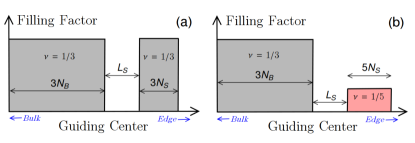
Figure 1: Schematic of two a priori possible configurations at the edge of the bulk $\nu=1/3$ phase. For a sharp confining potential, there is a single ($\nu=1/3$) quantum Hall droplet. For smoother edge potentials, an additional side strip, with filling factor (a) $1/3$ or (b) $1/5$, composed of $N_{S}$ electrons may be nucleated along the edge. The side strip is separated from the bulk (comprising $N_{B}$ electrons) by $L_{S}$ guiding centers.

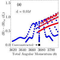
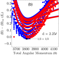
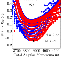
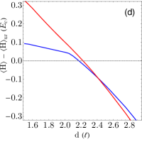
Figure 2: Results of the variational calculations with 50 electrons. (a)-(c) The energy ($\langle H\rangle$) of the states in the two variational classes as a function of the total angular momentum at (a) sharp ($d=0.01\ell$), (b) moderately smooth ($d=2.25\ell$), and (c) very smooth ($d=2.50\ell$) confining potentials, where $\ell$ is the magnetic length. In all cases, the energy of the unreconstructed state ($\langle H\rangle_{\text{ur}}$) has been subtracted. The blue (red) circles show energy of states with a side strip of $\nu=1/3$ ($\nu=1/5$). The black square marks the state with the lowest energy. (d) The lowest possible energy in the two variational classes as a function of the smoothness of the confining potential (parameterized by $d/\ell$). The blue (red) line corresponds to states with a side strip of $\nu=1/3$ ($\nu=1/5$). For sharp edges the ground state is the unreconstructed $\nu=1/3$ state with angular momentum $3675\hbar$. This state supports a single chiral $e/3$ mode. For moderately smooth potentials ($2.17<d/\ell<2.42$), an additional $\nu=1/3$ side strip is nucleated, which defines a pair of counterpropagating $e/3$ modes (in addition to the chiral $e/3$ mode arising from the bulk). For very smooth potentials ($d>2.42\ell$), a $\nu=1/5$ side strip is generated, which supports a pair of $e/5$ edge modes.

Our challenge here is to account theoretically for the reconstruction and, subsequently, renormalization, of the edge of a Laughlin state (specifically, $\nu=1/3$). To reach this goal, we need to determine the precise filling factor of the additional side strip nucleated at a smooth edge. Figure 1 depicts two a priori possible edge configurations, which are considered in our analysis fno . We stress that there is a qualitative difference between these two edge structures. The additional side strip of filling factor $1/3$ ($1/5$) defines counterpropagating modes of charge $e/3$ ($e/5$). For the case of $1/3$ side strip [Fig. 1(a)], subsequent renormalization of the modes (due to disorder-induced tunneling) would lead to localization of a pair of counterpropagating modes and may render transport experiments blind to the presence of reconstruction. On the other hand, for the $1/5$ strip [Fig. 1(b)], subsequent renormalization of the original $e/3$ mode and the upstream $e/5$ mode would not induce localization, and (as we demonstrate here) would have clear experimental manifestations. Our analysis identifies which structure is energetically preferable in a given parameter range.

Exact diagonalization Wan et al. (2002, 2003); Hu et al. (2008, 2009), being limited to small system sizes, does not allow us to obtain a quantized filling factor at the edge. We stress that such an analysis cannot clearly resolve the precise configuration of the edge, and, in particular, is unable to predict whether upstream neutral modes do or do not emerge upon reconstruction. For this reason, we employ a variational analysis to study the edge Meir (1994); Khanna et al. (2021), which overcomes these size limitations, while fully accounting for quantum correlations, inherently present in the Laughlin state. Specifically, we treat the strip-size ($N_{S}$) and separation ($L_{S}$) (cf. Fig. 1) as variational parameters, and evaluate the energy of the states in both configurations as a function of the confining potential slope. When the confining potential is sharp, there is no edge reconstruction, i.e., the lowest energy structure corresponds to $N_{S}=0$. As shown in Fig. 2, for moderately smooth potentials, an additional side strip comprising a $\nu=1/3$ phase emerges, while for even smoother potentials, the filling factor of the side strip becomes $\nu=1/5$. The edge modes of the latter structure, and their ensuing renormalization leading to the emergence of neutral modes, may account for the experimental results reported in Refs. Inoue et al. (2014); Bhattacharyya et al. (2019).

Our results for the reconstructed edge structure may be verified in carefully designed transport experiments. Consider, for instance, the behavior of the two-terminal conductance ($g_{\text{2-ter}}$) as a function of the sample length. With a single gapless mode, $g_{\text{2-ter}}$ is independent of the sample length and is determined solely by the bulk filling factor (in this case $g_{\text{2-ter}}=1/3\times e^{2}/h$). For reconstructed edges, though, the conductance may vary with the sample length Spånslätt et al. (2021) due to intermode equilibration facilitated by interactions and disorder-induced tunneling Protopopov et al. (2017); Nosiglia et al. (2018). For sufficiently long samples (with full edge equilibration), $g_{\text{2-ter}}=1/3\times e^{2}/h$ for any edge structure. For shorter samples (with no intermode equilibration), $g_{\text{2-ter}}$ assumes the value $1\times e^{2}/h$ ($11/15\times e^{2}/h$) for a side strip of filling factor 1/3 (1/5). Furthermore, for the configuration with a $\nu=1/5$ side strip, disorder-induced random tunneling and intermode interactions between the counterpropagating $e/3$ and $e/5$ modes lead to the emergence of new effective modes (Fig. 3), which, upon renormalization, may comprise upstream neutral modes. The experimental consequences of the emergence of such nontopological neutrals are similar to those discussed above for the case of hole-conjugate QH states.

Model.–We analyze the edge of the $\nu=1/3$ state in the disk geometry. The Hilbert space is restricted to the lowest Landau level and we assume spin-polarized electrons. In this limit, the bulk $\nu=1/3$ state is well described by the Laughlin wave function Laughlin (1983); Jain (2007)

$$\Psi_{\frac{1}{3},N}=\prod_{i=1}^{N}\bigg{[}\prod_{j>i}\big{(}z_{i}-z_{j}\big{)}^{3}\bigg{]}e^{-\frac{1}{4}\sum_{i}|z_{i}|^{2}},$$ (1)

where $N$ is the number of electrons, $z_{j}=(x_{j}-iy_{j})/\ell$ is the position of $j{\text{th}}$ electron and $\ell$ is the magnetic length. The Hamiltonian of the system is $H=H_{\text{ee}}+H_{\text{c}}$, where $H_{\text{ee}}$ is the electronic repulsion and $H_{\text{c}}$ is the confining potential (assumed to be circularly symmetric). Since $H$ is rotationally invariant, the many-body variational states may be classified using the total angular momentum.

We assume the electrons interact via the long-range Coulomb interaction ($\frac{e^{2}}{4\pi\epsilon_{0}}\sum_{i\neq j}1/|\vec{r}_{i}-\vec{r}_{j}|$). The confining potential is modeled as the electrostatic potential of a positively charged background disk separated from the electron gas by a distance $d$ along the magnetic field Wan et al. (2002, 2003). The density and radius of the background disk are fixed such that the full system is charge neutral Sup . The slope of the ensuing potential is controlled by $d/\ell$, which is our tuning parameter. The potential is quite sharp for $d\sim 0$, and becomes smoother as $d$ increases. In our model $E_{\text{c}}=\frac{e^{2}}{4\pi\epsilon_{0}\ell}$ sets the energy scale for both the electronic repulsion and the confining potential, and hence drops out of the analysis.

Variational analysis.–Figure 1 shows the two classes of variational states considered here to describe the reconstructed edge of a $\nu=1/3$ Laughlin state. Both classes represent product states ($|\Psi_{\frac{1}{3},N_{B}}\rangle\otimes|\Psi_{\frac{1}{m_{S}},N_{S},M_{S}}\rangle$) of the bulk and a single edge strip. The edge strip comprising $N_{S}$ electrons is described by a $\nu=1/m_{S}$ Laughlin state ($m_{S}=3,5$) with $M_{S}$ quasiholes at the center. The corresponding (unnormalized) wave function is Laughlin (1983); Jain (2007)

$$\Psi_{\frac{1}{m_{S}},N_{S},M_{S}}=\prod_{i=1}^{N_{S}}\bigg{[}z_{i}^{M_{S}}\bigg{]}\bigg{[}\prod_{j>i}\big{(}z_{i}-z_{j}\big{)}^{m_{S}}\bigg{]}e^{-\frac{1}{4}\sum_{i}|z_{i}|^{2}}.$$ (2)

In our analysis, the total number of electrons ($N_{B}+N_{S}$) is fixed (to be 50 here). The number of electrons in the strip ($N_{S}$) and the number of unoccupied guiding centers between the bulk and the strip ($L_{S}=M_{S}+2-3N_{B}$) are the two parameters that label the states in both the classes considered here. The energy ($\langle H\rangle$) of these states may be evaluated as a function of $d$, using standard classical Monte Carlo techniques Sup . The unreconstructed state (without an additional edge strip) is included in both classes (corresponding to $N_{S}=0$). It is the lowest energy state for sharp confining potentials. By contrast, the ground state supports an additional edge strip (finite $N_{S}$ and $L_{S}$) for smoother potentials. The precise filling factor of this strip (and the nature of the additional counterpropagating modes) may be determined by comparing the energies of the states in the two classes.

Results.–Figure 2 depicts the energy ($\langle H\rangle$) of the states in both classes, labeled by the total angular momentum, for several values of $d$, which controls the sharpness of the confining potential. The blue (red) dots [in Figs. 2(a)-(c)] correspond to edges with a $\nu=1/3$ ($\nu=1/5$) side strip. The black square marks the lowest energy state. In all cases, the energy of the unreconstructed state was subtracted to ease the comparison. For a sharp confining potential [$d\lessapprox 2.1\ell$, Fig. 2(a)] the Laughlin state (with no additional side strip), supporting a single chiral $e/3$ edge mode, has the lowest energy (as expected).

The lowest energy state at smoother potentials [$d\gtrapprox 2.1\ell$] comprises an additional side strip. This side strip may have filling factor $1/3$ [Fig. 2(b)] for a moderately smooth potential ($N_{S}=15,L_{S}=11\text{ for }d=2.25\ell$) or $1/5$ [Fig. 2(c)] for very shallow potential ($N_{S}=14,L_{S}=3\text{ for }d=2.5\ell$). Figure 2(d) shows the variation of the lowest possible energy in the two classes with the confining potential slope. Evidently, the side strip filling factor is $1/3$ in the range $2.17\ell<d<2.42\ell$, and switches to $1/5$ for larger $d$. The reconstructed edge configurations support, in addition to the single $e/3$ mode arising from the bulk, a pair of counterpropagating $e/3$ or $e/5$ modes. In the rest of this Letter, we focus on the experimental manifestations of these additional counterpropagating modes.

Transport signatures–two terminal conductance.–The various edge structures obtained in our numerical analysis may be identified through their unique signatures in designed transport experiments. The (electric) two terminal conductance ($g_{\text{2-ter}}$) as a function of the length of the edge ($L$) is one such measurement. There, in the absence of edge equilibration, the chiral channels exiting the source contact are biased with respect to the modes entering it. The presence of impurities and potential disorder generates random tunneling between the (co- and counterpropagating) modes at the edge, which may facilitate intermode equilibration over a characteristic length $\ell_{\text{eq}}$. For $L\gg\ell_{\text{eq}}$, the two-terminal conductance is $g_{\text{2-ter}}=1/3\times e^{2}/h$ irrespective of the confining potential slope, reflecting the bulk filling factor.

More interesting is the $L\ll\ell_{\text{eq}}$ regime, where $g_{\text{2-ter}}$ is sensitive to the detailed structure of the edge. For the unreconstructed edge, $g_{\text{2-ter}}=1/3\times e^{2}/h$ for all values of $L$; the presence of a single chiral $1/3$ mode implies that the notion of equilibration is irrelevant. For reconstructed edges the additional pair of counterpropagating modes also contribute to $g_{\text{2-ter}}$. For an edge comprising a $\nu=1/3$ side stripe, $g_{\text{2-ter}}=1\times e^{2}/h$ ($1/3\times 3$). For a $\nu=1/5$ side strip, $g_{\text{2-ter}}=11/15\times e^{2}/h$ ($1/3+2\times 1/5$). Such unequilibrated counterpropagating modes have been reported for other bulk filling fractions Lafont et al. (2019).

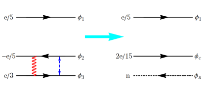
Figure 3: For the edge structure with a $\nu=1/5$ strip, interactions (represented by the red curve) and disorder-induced electron tunneling (blue dashed line) between the inner two edge modes may lead to emergence of a renormalized downstream charge ($\phi_{c}$) and an upstream neutral mode ($\phi_{n}$). The outermost mode is assumed to be completely decoupled from the inner two modes. This idealization is justified by the variational analysis, which shows that as the confining potential becomes shallower, the width of the side strip (proportional to $N_{S}$) increases faster than the separation of the strip ($L_{S}$).

Plateaus in conductance through a QPC.–The existence of counterpropagating $1/5$ modes at the edge of a bulk $1/3$ state may also be detected through measurement of the conductance across a QPC. For a $\nu=1/3$ bulk phase, the conductance through a fully open QPC (transmission = 1) is expected to be $1/3\times e^{2}/h$ (assuming full electrical equilibration). If the edge comprises an additional $\nu=1/5$ strip and in the absence of strong edge renormalization, one may pinch-off the QPC such that the innermost $1/3$ and the upstream $1/5$ modes are fully reflected, and only the outermost $1/5$ mode is transmitted. Then a conductance plateau at $1/5\times e^{2}/h$ is expected. As the bulk filling factor does not deviate while tuning the QPC, this would be a smoking-gun signature of the presence of a $1/5$ strip at the edge of a bulk $1/3$ phase.

Neutral modes.–Consider the reconstructed edge with a $\nu=1/5$ side strip. The low energy dynamics of the three chiral modes may be described by (chiral) bosonic fields $\phi_{j}$ for $j=1,2,3$ (outermost being 1 and the innermost being 3) Wen (2007, 1990, 1992). The fields satisfy the Kac-Moody algebra, $[\phi_{j_{1}}(x),\phi_{j_{2}}(x^{\prime})]=i\pi\delta_{j_{1}j_{2}}K^{-1}_{j}\text{sgn}(x-x^{\prime})$, where the elements of the $K$ matrix are $K_{1}=5,K_{2}=-5,K_{3}=3$. These bare edge modes may undergo subsequent renormalization due to disorder-induced tunneling and intermode interactions. Our variational analysis indicates that for sufficiently smooth potentials, the outermost downstream $e/5$ mode would be located far from the inner two modes and hence, couple very weakly with those. This motivates the idealization that $\phi_{1}$ is completely decoupled from $\phi_{2,3}$ (cf. Fig. 3). The inner modes correspond to an upstream $e/5$ mode ($\phi_{2}$) and a downstream $e/3$ mode ($\phi_{3}$). Because of the unequal charges, this pair of counterpropagating modes cannot be localized by disorder-induced backscattering. Instead, the renormalized modes support excitations with generic (nonuniversal) charges $e_{u}$ and $e_{d}$ Protopopov et al. (2017), where $u$ and $d$ denote the upstream and downstream direction, respectively. Interestingly, under certain conditions, the upstream mode may be charge neutral, i.e., $e_{u}=0$. In this case, the bulk-boundary correspondence dictates that $e_{d}=2e/15$. The emergent edge structure thus consists of two downstream modes $\phi_{1}$ (with charge $e/5$) and $\phi_{c}$ (charge $2e/15$) and one upstream neutral mode $\phi_{n}$.

The emergent $\phi_{n}$ mode has several experimental consequences. It may lead to an upstream heat flow without an accompanying charge current. Such observations, consistent with either charge equilibration or the presence of a coherent neutral mode, were reported in Refs. Inoue et al. (2014); Venkatachalam et al. (2012). Another major consequence is that neutral modes may suppress the visibility of anyonic interference in electronic Mach-Zehnder setups Goldstein and Gefen (2016), as was reported in Ref. Bhattacharyya et al. (2019). Finally, consider the QPC setup discussed previously, which may be tuned to a quantized conductance plateau of $1/5$. Because of the presence of counterpropagating modes (which are fully reflected at the QPC), the system may exhibit shot noise even though the conductance is quantized; the ensuing Fano factor may also be quantized if certain conditions are satisfied Spånslätt et al. (2020); Park et al. (2021).

Conclusions.–Transport measurements Bhattacharyya et al. (2019); Inoue et al. (2014) suggest that the orthodox edge models Wen (1990, 1992, 2007) do not hold even for relatively simple QH states. Specifically, experiments point to the presence of upstream mode(s) at the edge of a bulk $1/3$ state. Motivated by this surprising finding, here we study the edge structure of the $\nu=1/3$ Laughlin state as a function of the slope of the boundary confining potential. We find that an additional incompressible side strip is nucleated for sufficiently smooth potentials. Such a configuration allows the coarse-grained electronic density to follow the confining potential, while at the same time facilitating the formation of gapped QH states locally. Our analysis reveals that the filling factor of this side strip depends on the slope of the confining potential. For a moderate slope, a $\nu=1/3$ side strip arises while for a sufficiently small slope the side strip is described by $\nu=1/5$. The latter structure supports three gapless chirals: an $e/3$ downstream mode and a counterpropagating pair of $e/5$ modes. Subsequent renormalization, driven by intermode interactions and disorder-induced-tunneling among the downstream $e/3$ and upstream $e/5$ modes, may lead to the emergence of an upstream neutral mode, and may account for the observations of Refs. Bhattacharyya et al. (2019); Inoue et al. (2014). We also discuss additional experimental manifestations for the reconstructed edge structures. We expect that edge stripes with more complex structure may arise upon fine-tuning the interplay between interaction and confining potential. Detailed investigations along these lines, including in engineered geometries Ronen et al. (2018); Cohen et al. (2019b), is left to future work.

Supplemental Material for “Emergence of Neutral Modes in Laughlin-like Fractional Quantum Hall Phases” Udit Khanna

Moshe Goldstein Yuval Gefen

Basic Setup

We employ the disk geometry to analyze the edge of the $\nu=1/3$ state and use a rotationally symmetric gauge, $e\vec{A}/\hbar=(-y/2\ell^{2},x/2\ell^{2})$, where $\ell=\sqrt{\hbar/eB}$ is the magnetic length. Due to the rotational symmetry of the system, the single-particle states may be labelled by eigenvalues of the angular momentum ($\hat{L}$). We denote the states in the lowest Landau level (LLL) as $\phi_{m}$ with $m=0,1,2,\dots$. The corresponding wavefunction is $\phi_{m}(\vec{r}\,)=\left(r/\ell\right)^{m}e^{-im\theta_{\text{r}}}e^{-\left(\frac{r}{2\ell}\right)^{2}}/\sqrt{2^{m+1}\pi m!\ell^{2}}$, where $re^{-i\theta_{\text{r}}}=x-iy$ is the position of the electron. The state $\phi_{m}$ is strongly localized around $r=\sqrt{2m}\ell$ and has angular momentum $\hbar m$.

Restricting the Hilbert space to LLL and ignoring electronic spin, the Hamiltonian is $H=H_{\text{ee}}+H_{\text{c}}$, where $H_{\text{ee}}$ is the electronic interaction and $H_{\text{c}}$ is the edge confining potential (assumed to be rotationally symmetric). Note that $H$ commutes with $\hat{L}$. Therefore, the total angular momentum may be used to label the many-body states in our analysis. Defining $E_{c}=e^{2}/\epsilon_{0}\ell$ as the Coulomb energy scale and $c_{m}$ as the annihilation operator corresponding to $\phi_{m}$, we have,

$$H_{\text{ee}} =\frac{E_{\text{c}}}{2}\sum_{i\neq j}\frac{\ell}{|\vec{r}_{i}-\vec{r}_{j}|}$$ (S1)

$$\equiv\frac{E_{\text{c}}}{2}\sum_{m_{1},m_{2},n}V_{m_{1}m_{2};n}^{ee}c_{m_{1}+n}^{\dagger}c_{m_{2}}^{\dagger}c_{m_{2}+n}c_{m_{1}},$$ (S2)

$$H_{\text{c}} =\sum_{m}V_{m}^{\text{c}}\,\,c_{m}^{\dagger}c_{m}.$$ (S3)

To model the edge potential, we consider a uniformly charged disk with radius $R$ and positive charge density $\sigma$, located a distance $d$ away from the electronic plane Zhang and Yang (2013); Wan et al. (2002, 2003). The electrostatic potential of this disk on the electrons is given by,

$$V_{c}(r)=\int_{0}^{R}dr^{\prime}\int_{0}^{2\pi}d\theta\frac{E_{c}\sigma}{\sqrt{d^{2}+r^{2}+{r^{\prime}}^{2}-2r^{\prime}r\cos\theta}}.$$ (S4)

$V_{m}^{\text{c}}$ in Eq. (S3) are the matrix elements of $V_{c}(r)$. We use $\sigma=(1/3)/2\pi\ell^{2}$ and $R^{2}=2(N_{S}+N_{B})\ell^{2}$, in order to maintain overall charge neutrality. For $d=0$ this confining potential is very sharp, and it get shallower as $d$ increases.

Variational Analysis

Figure 1 depicts the two classes of variational states considered in this work. Both classes represent the product state of a bulk $\nu=1/3$ state with an annulus of the $\nu=1/m_{S}$ state ($m_{S}=3,5$). The bulk state (denoted as $|\psi_{\frac{1}{3},N_{B}}\rangle$) comprises $N_{B}$ electrons and is well described by the (unnormalized) Laughlin wavefunction Laughlin (1983)

$$\Psi_{\frac{1}{3},N_{B}}=\prod_{i=1}^{N_{B}}\bigg{[}\prod_{j>i}\big{(}z_{i}-z_{j}\big{)}^{3}\bigg{]}e^{-\frac{1}{4}\sum_{i}|z_{i}|^{2}}.$$ (S5)

Here $z_{j}=(x_{j}-iy_{j})/\ell$ is coordinate of the $j^{\text{th}}$ electron. The annulus state (denoted as $|\psi_{\frac{1}{m_{S}},N_{S},M_{S}}\rangle$) is a $\nu=1/m_{S}$ Laughlin state consisting of $N_{S}$ electrons and $M_{S}$ quasiholes at the origin. The corresponding wavefunction may be written as,

$$\Psi_{\frac{1}{m_{S}},N_{S},M_{S}}=\prod_{i=1}^{N_{S}}\bigg{[}z_{i}^{M_{S}}\bigg{]}\bigg{[}\prod_{j>i}\big{(}z_{i}-z_{j}\big{)}^{m_{S}}\bigg{]}e^{-\frac{1}{4}\sum_{i}|z_{i}|^{2}}.$$ (S6)

Note that the single-particle state with smallest angular momentum which may be occupied in the annulus state is $\phi_{M_{S}}$. Then if $L_{S}$ denotes the number of guiding centers between the bulk and annulus state, we have $M_{S}=3N_{B}-2+L_{S}$.

The angular momentum (in units of $\hbar$) of the ($\nu=1/m$) Laughlin state with $N$ particles is $\frac{m}{2}N(N-1)$. Introducing $M$ quasiholes at the origin increases the angular momentum by $NM$. Then the total angular momentum of a product state with a $\nu=1/m_{S}$ side strip is

$$\frac{3}{2} (N_{B}+N_{S})(N_{B}+N_{S}-1)$$

$$+\frac{m_{S}-3}{2}N_{S}(N_{S}-1)+N_{S}(L_{S}-2).$$ (S7)

The first term above is the angular momentum of the unreconstructed state. This indicates that the variational states may have angular momentum smaller than that of the unreconstructed state if $L_{S}$ is sufficiently small. However, compressing a Laughlin state would increase the Coulomb repulsion and therefore the energy of such states is unlikely to be lower than that of the unreconstructed state.

The energy ($\langle H\rangle$) of the product states is the sum of the energy of the individual components and their mutual interaction energy. The energy of individual components is,

$$\frac{1}{\int\prod_{i}d^{2}r_{i}\big{|}\Psi\big{|}^{2}} \int\prod_{i}d^{2}r_{i}\big{|}\Psi\big{|}^{2}\bigg{[}\sum_{i<j}\frac{E_{c}\ell}{|\vec{r}_{i}-\vec{r}_{j}|}\bigg{]}$$

$$+E_{c}\sum_{m}\langle c_{m}^{\dagger}c_{m}\rangle_{\Psi}V_{m}^{c}.$$ (S8)

where $\langle c_{m}^{\dagger}c_{m}\rangle_{\Psi}$ is the occupation of the single-particle states in each component. The mutual interaction energy of the bulk ($\Psi_{B}$) and strip ($\Psi_{S}$) components is,

$$E_{c}\sum_{i\in\text{B}}\sum_{j\in\text{S}}\langle c_{i}^{\dagger}c_{i}\rangle_{\Psi_{\text{B}}}\langle c_{j}^{\dagger}c_{j}\rangle_{\Psi_{\text{S}}}\bigg{(}V_{ij;0}^{ee}-V_{ii;j-i}^{ee}\bigg{)}.$$ (S9)

The Coulomb energy of each component maybe evaluated using the standard Metropolis algorithm Metropolis et al. (1953); Laughlin (1983); Jain (2007). The average occupation may be evaluated similarly Mitra and MacDonald (1993); Khanna et al. (2021).

References

- Zhang and Yang (2013) Y. Zhang and K. Yang, Edge spin excitations and reconstructions of integer quantum Hall liquids, Phys. Rev. B 87, 125140 (2013).
- Wan et al. (2002) X. Wan, K. Yang, and E. H. Rezayi, Reconstruction of fractional quantum Hall edges, Phys. Rev. Lett. 88, 056802 (2002).
- Wan et al. (2003) X. Wan, E. H. Rezayi, and K. Yang, Edge reconstruction in the fractional quantum Hall regime, Phys. Rev. B 68, 125307 (2003).
- Laughlin (1983) R. B. Laughlin, Anomalous quantum Hall effect: An incompressible quantum fluid with fractionally charged excitations, Phys. Rev. Lett. 50, 1395 (1983).
- Metropolis et al. (1953) N. Metropolis, A. W. Rosenbluth, M. N. Rosenbluth, A. H. Teller, and E. Teller, Equation of state calculations by fast computing machines, The Journal of Chemical Physics 21, 1087 (1953).
- Jain (2007) J. K. Jain, Composite Fermions (Cambridge University Press, Cambridge, 2007).
- Mitra and MacDonald (1993) S. Mitra and A. H. MacDonald, Angular-momentum-state occupation-number distribution function of the Laughlin droplet, Phys. Rev. B 48, 2005 (1993).
- Khanna et al. (2021) U. Khanna, M. Goldstein, and Y. Gefen, Fractional edge reconstruction in integer quantum Hall phases, Phys. Rev. B 103, L121302 (2021).