Accelerating Perturbed Stochastic Iterates in Asynchronous Lock-Free Optimization

Abstract

We show that stochastic acceleration can be achieved under the perturbed iterate framework (Mania et al.,, 2017) in asynchronous lock-free optimization, which leads to the optimal incremental gradient complexity for finite-sum objectives. We prove that our new accelerated method requires the same linear speed-up condition as the existing non-accelerated methods. Our core algorithmic discovery is a new accelerated SVRG variant with sparse updates. Empirical results are presented to verify our theoretical findings.

1 Introduction

We consider the following unconstrained optimization problem, which appears frequently in machine learning and statistics, such as empirical risk minimization:

$$\min_{x\in\mathbb{R}^{d}}{f(x)\triangleq\frac{1}{n}\sum_{i=1}^{n}{f_{i}(x)}},$$ (1)

where each $f_{i}$ is $L$-smooth and convex, $f$ is $\mu$-strongly convex. We further assume that the computation of each $f_{i}$ is sparse, i.e., the computation is supported on a set of coordinates $T_{i}\subseteq\{1,\ldots,d\}$. For example, generalized linear models (GLMs) satisfy this assumption. GLMs has the form: $\forall i,f_{i}(x)=\ell_{i}(\left\langle a_{i},x\right\rangle)$, where $\ell_{i}$ is some loss function and $a_{i}\in\mathbb{R}^{d}$ is a data sample. In this case, the support of each $f_{i}$ is the set of non-zero coordinates of $a_{i}$. Many large real-world datasets have very high sparsity (see Table 1 for several examples).

In the past decade, exciting progress has been made on solving problem (1) with the introduction of stochastic variance reduced methods, such as SAG (Roux et al.,, 2012; Schmidt et al.,, 2017), SVRG (Johnson and Zhang,, 2013; Xiao and Zhang,, 2014), SAGA (Defazio et al.,, 2014), S2GD (Konečnỳ and Richtárik,, 2013), SARAH (Nguyen et al.,, 2017), etc. These methods achieve fast linear convergence rate as gradient descent (GD), while having low iteration cost as stochastic gradient descent (SGD). There are also several recent works on further improving the practical performance of these methods based on past gradient information (Hofmann et al.,, 2015; Tan et al.,, 2016; Shang et al.,, 2018; Shi et al.,, 2021; Dubois-Taine et al.,, 2021). Inspired by Nesterov’s seminal works (Nesterov,, 1983, 2003, 2018), stochastic accelerated methods have been proposed these years (Allen-Zhu,, 2017; Zhou et al.,, 2018, 2019; Zhou et al., 2020a, ; Lan et al.,, 2019; Song et al.,, 2020; Li,, 2021). These methods achieve the optimal convergence rates that match the lower complexity bounds established in (Woodworth and Srebro,, 2016). For sparse problems, lagged update (Schmidt et al.,, 2017) is a common technique for the above methods to efficiently leverage the sparsity.

Inspired by the emerging parallel computing architectures such as multi-core computer and distributed system, many parallel variants of the aforementioned methods have been proposed, and there is a vast literature on those attempts. Among them, asynchronous lock-free algorithms are of special interest. Recht et al., (2011) proposed an asynchronous lock-free variant of SGD called Hogwild! and first proved that it can achieve a linear speed-up, i.e., running Hogwild! with $\tau$ parallel processes only requires $O(1/\tau)$-times the running time of the serial variant. The condition on the maximum overlaps among the parallel processes is called the linear speed-up condition. Following Recht et al., (2011), Sa et al., (2015); Lian et al., (2015) analyzed asynchronous SGD for non-convex problems, and Duchi et al., (2013) analyzed for stochastic optimization; Mania et al., (2017) refined the analysis framework (called the perturbed iterate framework) and proposed KroMagnon (asynchronous SVRG); Leblond et al., (2017) simplified the perturbed iterate analysis and proposed ASAGA (asynchronous SAGA), and in the journal version of this work, Leblond et al., (2018) further improved the analysis of KroMagnon and Hogwild!; Pedregosa et al., (2017) derived proximal variant of ASAGA; Nguyen et al., (2018) refined the analysis of Hogwild!; Joulani et al., (2019) proposed asynchronous methods in online and stochastic settings; Gu et al., (2020) proposed several asynchronous variance reduced algorithms for non-smooth or non-convex problems; Stich et al., (2021) studied a broad variety of SGD variants and improved the speed-up condition of asynchronous SGD.

All the above mentioned asynchronous methods are based on non-accelerated schemes such as SGD, SVRG and SAGA. Witnessing the success of recently proposed stochastic accelerated methods, it is natural to ask: Is it possible to achieve stochastic acceleration in asynchronous lock-free optimization? Will it lead to a worse linear speed-up condition? The second question comes from a common perspective that accelerated methods are less tolerant to the gradient noise, e.g., (Devolder et al.,, 2014; Cyrus et al.,, 2018).

In this work, we give positive answers to these questions, i.e., we propose the first asynchronous stochastic accelerated method for solving problem (1), and we prove that it requires the identical linear speed-up condition as the non-accelerated counterparts.

The works that are closest related to us are (Fang et al.,, 2018; Zhou et al.,, 2018; Hannah et al.,, 2019). Fang et al., (2018) proposed several asynchronous accelerated schemes. However, their analysis requires consistent read and does not consider sparsity. The dependence on the number of overlaps $\tau$ in their complexities is $O(\tau)$ compared with $O(\sqrt{\tau})$ in our result. Zhou et al., (2018) naively extended their proposed accelerated method into asynchronous lock-free setting. However, even in the serial case, their result imposes strong assumptions on the sparsity. This issue is discussed in detail in Section 3.1. In the asynchronous case, no theoretical acceleration is achieved in (Zhou et al.,, 2018). Hannah et al., (2019) proposed the first asynchronous accelerated block-coordinate descent method (BCD). However, as pointed out in Appendix F in (Pedregosa et al.,, 2017), BCD methods perform poorly in sparse problems since they focus only on a single coordinate of the gradient information.

2 Preliminaries

Notations

We use $\left\langle\cdot,\cdot\right\rangle$ and $\left\lVert\cdot\right\rVert$ to denote the standard inner product and the Euclidean norm, respectively. We let $[n]$ denote the set $\{1,2,\ldots,n\}$, $\mathbb{E}$ denote the total expectation and $\mathbb{E}_{i}$ denote the expectation with respect to a random sample $i$. We use $[x]_{v}$ to denote the coordinate $v$ of the vector $x\in\mathbb{R}^{d}$, and for a subset $T\subseteq[d]$, $[x]_{T}$ denotes the collection of $[x]_{v}$ for $v\in T$. We let $\lceil\cdot\rceil$ denote the ceiling function, $I_{d}$ denote the identity matrix and $(\alpha)_{+}\triangleq\max{\{\alpha,0\}}$.

We say that a function $f:\mathbb{R}^{d}\rightarrow\mathbb{R}$ is $L$-smooth if it has $L$-Lipschitz continuous gradients, i.e., $\forall x,y\in\mathbb{R}^{d}$,

$$\left\lVert\nabla f(x)-\nabla f(y)\right\rVert\leq L\left\lVert x-y\right\rVert.$$

An important consequence of $f$ being $L$-smooth and convex is that $\forall x,y\in\mathbb{R}^{d}$,

$$f(x)-f(y)-\left\langle\nabla f(y),x-y\right\rangle\geq{}\frac{1}{2L}\left\lVert\nabla f(x)-\nabla f(y)\right\rVert^{2}.$$

We call it the interpolation condition following (Taylor et al.,, 2017). A continuously differentiable $f$ is called $\mu$-strongly convex if $\forall x,y\in\mathbb{R}^{d}$,

$$f(x)-f(y)-\left\langle\nabla f(y),x-y\right\rangle\geq\frac{\mu}{2}\left\lVert x-y\right\rVert^{2}.$$

In particular, the strong convexity at any $x\in\mathbb{R}^{d}$ and $x^{\star}$ is called the quadratic growth, i.e.,

$$f(x)-f(x^{\star})\geq\frac{\mu}{2}\left\lVert x-x^{\star}\right\rVert^{2}.$$

All our results hold under this weaker condition. We define $\kappa\triangleq\frac{L}{\mu}$, which is always called the condition ratio. Other equivalent definitions of these assumptions can be found in (Nesterov,, 2018; Karimi et al.,, 2016).

Oracle complexity refers to the number of incremental gradient computations needed to find an $\epsilon$-accurate solution (in expectation), i.e., $\mathbb{E}\left[f(x)\right]-f(x^{\star})\leq\epsilon$.

3 Serial Sparse Accelerated SVRG

We first introduce a new accelerated SVRG variant with sparse updates in the serial case (Algorithm 1), which serves as the base algorithm for our asynchronous scheme. Our technique is built upon the following sparse approximated SVRG gradient estimator proposed in (Mania et al.,, 2017): For uniformly random $i\in[n]$ and $y,\tilde{x}\in\mathbb{R}^{d}$, define

$$\mathcal{G}_{y}\triangleq\nabla f_{i}(y)-\nabla f_{i}(\tilde{x})+D_{i}\nabla f(\tilde{x}),$$ (2)

where $D_{i}\triangleq P_{i}D$ with $P_{i}\in\mathbb{R}^{d\times d}$ being the diagonal projection matrix of $T_{i}$ (the support of $f_{i}$) and $D=(\frac{1}{n}\sum_{i=1}^{n}{P_{i}})^{-1}$, which can be computed and stored in the first pass. Note that we assume the coordinates with zero cardinality have been removed in the objective function, and thus $nI_{d}\succeq D\succeq I_{d}$. A diagonal element of $D$ corresponds to the inverse probability of the coordinate belonging to a uniformly sampled support $T_{i}$. It is easy to verify that this construction ensures the unbiasedness $\mathbb{E}_{i}\big{[}D_{i}\nabla f(\tilde{x})\big{]}=\nabla f(\tilde{x})$.

This section is organized as follows: In Section 3.1, we summarize the key technical novelty and present the convergence result; in Section 3.2, we remark on the design of Algorithm 1; in Section 3.3, we briefly discuss its general convex variant.

3.1 Sparse Variance Correction

Algorithm 1 SS-Acc-SVRG: Serial Sparse Accelerated SVRG

1:initial guess $x_{0}\in\mathbb{R}^{d}$, constant $\omega>1$ which controls the restart frequency.

2:set the scalars $m,\vartheta,\varphi,\eta,S,R$ according to Theorem 1, initialize the diagonal matrix $D$.

3:for $r=0,\ldots,R-1$ do$\triangleright$ performing restarts

4:     $\tilde{x}_{0}=z^{0}_{0}=x_{r}$.

5:     for $s=0,\ldots,S-1$ do

6:         Compute and store $\nabla f(\tilde{x}_{s})$.

7:         for $k=0,\ldots,m-1$ do

8:              Sample $i_{k}$ uniformly in $[n]$ and let $T_{i_{k}}$ be the support of $f_{i_{k}}$.

9:               $[y_{k}]_{T_{i_{k}}}=\vartheta\cdot[z^{s}_{k}]_{T_{i_{k}}}+\left(1-\vartheta\right)\cdot[\tilde{x}_{s}]_{T_{i_{k}}}-\varphi\cdot[D\nabla f(\tilde{x}_{s})]_{T_{i_{k}}}.$ $\triangleright$ sparse coupling

10:               $[z^{s}_{k+1}]_{T_{i_{k}}}=[z^{s}_{k}]_{T_{i_{k}}}-\eta\cdot\big{(}\nabla f_{i_{k}}([y_{k}]_{T_{i_{k}}})-\nabla f_{i_{k}}([\tilde{x}_{s}]_{T_{i_{k}}})+D_{i_{k}}\nabla f(\tilde{x}_{s})\big{)}$.$\triangleright$ sparse update

11:         end for

12:         $\tilde{x}_{s+1}=y_{t}$ for uniformly random $t\in\{0,1,\ldots,m-1\}$.

13:         $z^{s+1}_{0}=z^{s}_{m}$.

14:     end for

15:     $x_{r+1}=\frac{1}{S}\sum_{s=0}^{S-1}{\tilde{x}_{s+1}}$.

16:end for

17:$x_{R}$.

Intuitively, the sparse SVRG estimator (2) will leads to a larger variance compared with the dense one (when $D=I_{d}$). In the previous attempt, Zhou et al., (2018) naively extends an accelerated SVRG variant into the sparse setting, which results in a fairly strong restriction on the sparsity as admitted by the authors. By contrast, sparse variants of SVRG and SAGA in (Mania et al.,, 2017; Leblond et al.,, 2017) require no assumption on the sparsity, and they achieve the same oracle complexities as their original dense versions.

Analytically speaking, the only difference of adopting the sparse estimator (2) is on the variance bound. The analysis of non-accelerated dense SVRG typically uses the following variance bound ($D=I_{d}$) (Johnson and Zhang,, 2013; Xiao and Zhang,, 2014):

$$\mathbb{E}\left[\left\lVert\mathcal{G}_{y}-\nabla f(y)\right\rVert^{2}\right]\leq 4L\big{(}f(y)-f(x^{\star})+f(\tilde{x})-f(x^{\star})\big{)}.$$

It is shown in (Mania et al.,, 2017) that the sparse estimator (2) admits the same variance bound for any $D$. Thus, the analysis in the dense case can be directly applied to the sparse variant, which leads to a convergence guarantee that is independent of the sparsity.

However, things are not as smooth in the accelerated case. To (directly) accelerate SVRG, we typically uses a much tighter variance bound in the form ($D=I_{d}$) (Allen-Zhu,, 2017):

$$\mathbb{E}\left[\left\lVert\mathcal{G}_{y}-\nabla f(y)\right\rVert^{2}\right]\!\leq 2L\big{(}f(\tilde{x})-f(y)-\left\langle\nabla f(y),\tilde{x}-y\right\rangle\big{)}.$$

Unfortunately, in the sparse case ($D\neq I_{d}$), we do not have an identical variance bound as before. The variance of the sparse estimator (2) can be bounded as follows. The proof is given in Appendix A.

Lemma 1 (Variance bound for accelerated SVRG).

The variance of $\mathcal{G}_{y}$ (defined at (2)) can be bounded as

$$\mathbb{E}_{i}\left[\left\lVert\mathcal{G}_{y}-\nabla f(y)\right\rVert^{2}\right]\leq{} 2L\big{(}f(\tilde{x})-f(y)-\left\langle\nabla f(y),\tilde{x}-y\right\rangle\big{)}\!-\!\left\lVert\nabla f(y)\right\rVert^{2}$$ (3)

$$+\underbrace{2\left\langle\nabla f(y),D\nabla f(\tilde{x})\right\rangle}_{\mathcal{R}_{1}}-\left\langle\nabla f(\tilde{x}),D\nabla f(\tilde{x})\right\rangle.$$

In general, except for the dense case, where we can drop the last three terms above by completing the square, this upper bound will always be correlated with the sparsity (i.e., $D$). This correlation causes the strong sparsity assumption in (Zhou et al.,, 2018). We may consider a more specific case where $D=nI_{d}$. In this case, the last three terms above can be written as $(n-1)\left\lVert\nabla f(y)\right\rVert^{2}-n\left\lVert\nabla f(y)-\nabla f(\tilde{x})\right\rVert^{2}$, which is not always non-positive.

Inspecting (3), we see that it is basically the term $\mathcal{R}_{1}$, which could be positive, that causes the issue. We thus propose a novel sparse variance correction for accelerated SVRG, which is designed to perfectly cancel $\mathcal{R}_{1}$. The correction is added to the coupling step (Step 9):

$$y_{k}=\vartheta\cdot z_{k}+\underbrace{\left(1-\vartheta\right)\cdot\tilde{x}_{s}}_{\text{Negative Momentum}}-\underbrace{\varphi\cdot D\nabla f(\tilde{x}_{s})}_{\text{Sparse Variance Correction}}.$$

This correction neutralizes all the negative effect of the sparsity, in a similar way as how the negative momentum cancels the term $\left\langle\nabla f(y),\tilde{x}-y\right\rangle$ in the analysis (Allen-Zhu,, 2017). We can understand this correction as a variance reducer that controls the additional sparse variance. Then we have the following sparsity-independent convergence result for Algorithm 1, and its proof is given in Appendix B.

Theorem 1.

For any constant $\omega>1$, let $m=\Theta(n),\vartheta=\frac{\sqrt{m}}{\sqrt{\kappa}+\sqrt{m}},\varphi=\frac{1-\vartheta}{L}$, $\eta=\frac{1-\vartheta}{L\vartheta}$ and $S=\left\lceil 2\omega\sqrt{\frac{\kappa}{m}}\right\rceil$. For any accuracy $\epsilon>0$, we restart $R=O\big{(}\log{\frac{f(x_{0})-f(x^{\star})}{\epsilon}}\big{)}$ rounds. Then, Algorithm 1 outputs $x_{R}$ satisfying $\mathbb{E}\left[f(x_{R})\right]-f(x^{\star})\leq\epsilon$ in oracle complexity

$$O\left(\max{\left\{n,\sqrt{\kappa n}\right\}}\log{\frac{f(x_{0})-f(x^{\star})}{\epsilon}}\right).$$

This complexity matches the lower bound established in (Woodworth and Srebro,, 2016) (up to a log factor), and is substantially faster than the $O\big{(}(n+\kappa)\log{\frac{1}{\epsilon}}\big{)}$ complexity of sparse approximated SVRG and SAGA derived in (Leblond et al.,, 2017, 2018) in the ill-conditioned regime ($\kappa\gg n$).

3.2 Other Remarks about Algorithm 1

• We adopt a restart framework to handle the strong convexity, which is also used in (Zhou et al.,, 2018) and is suggested in (Allen-Zhu,, 2017) (footnote 9). This framework allows us to relax the strong convexity assumption to quadratic growth. Other techniques for handling the strong convexity such as (i) assuming a strongly convex regularizer and using proximal update (Nesterov,, 2005; Allen-Zhu,, 2017), and (ii) the direct constructions in (Lan et al.,, 2019; Zhou et al., 2020b, ; Li,, 2021) fail to keep the inner iteration sparse, and we are currently not sure how to modify them.

• The restarting point $x_{r+1}$ is chosen as the averaged point instead of a uniformly random one because large deviations are observed in the loss curve if a random restarting point is used.

• We can also use the correction to fix the sparsity issue in (Zhou et al.,, 2018), which leads to a slightly different method and somewhat longer proof.

• Algorithm 1 degenerates to a strongly convex variant of Acc-SVRG-G proposed in (Zhou et al.,, 2021) in the dense case ($D=I_{d}$), which summarizes our original inspiration. Note that Acc-SVRG-G is designed for minimizing the gradient norm and function value at the same time, which has nothing to do with handling sparsity. Its correction is not necessary if we only want to minimize the function value at the optimal rate, unlike our correction.

3.3 General Convex Variant

A general convex ($\mu=0$) variant of Algorithm 1 can be derived by removing the restarts and adopting a variable parameter choice similar to Acc-SVRG-G in (Zhou et al.,, 2021), which leads to a similar rate. We also find that our correction can be used in Varag (Lan et al.,, 2019) and ANITA (Li,, 2021) in the general convex case. Since the previous works on asynchronous lock-free optimization mainly focus on the strongly convex case, we omit the discussion here.

Algorithm 2 AS-Acc-SVRG: Asynchronous Sparse Accelerated SVRG

1:initial guess $x_{0}\in\mathbb{R}^{d}$, constant $\omega>1$ which controls the restart frequency.

2:set $m,\vartheta,\varphi,\eta,S,R$ according to Theorem 2, initialize shared variable $z$ and diagonal matrix $D$.

3:for $r=0,\ldots,R-1$ do$\triangleright$ performing restarts

4:     $\tilde{x}_{0}=z=x_{r}$.

5:     for $s=0,\ldots,S-1$ do

6:         Compute in parallel and store $\nabla f(\tilde{x}_{s})$.

7:         while number of samples $\leq m$ do in parallel

8:              Sample $i$ uniformly in $[n]$ and let $T_{i}$ be the support of $f_{i}$.

9:              $[\hat{z}]_{T_{i}}=$ inconsistent read of $z$ on $T_{i}$.

10:              $[\hat{y}]_{T_{i}}=\vartheta\cdot[\hat{z}]_{T_{i}}+\left(1-\vartheta\right)\cdot[\tilde{x}_{s}]_{T_{i}}-\varphi\cdot[D\nabla f(\tilde{x}_{s})]_{T_{i}}.$

11:              $[u]_{T_{i}}=-\eta\cdot\big{(}\nabla f_{i}([\hat{y}]_{T_{i}})-\nabla f_{i}([\tilde{x}_{s}]_{T_{i}})+D_{i}\nabla f(\tilde{x}_{s})\big{)}$.

12:              for $v\in T_{i}$ do

13:                  $[z]_{v}=[z]_{v}+[u]_{v}$. $\triangleright$ coordinate-wise atomic write

14:              end for

15:         end while

16:         $\tilde{x}_{s+1}=\hat{y}_{t}$, where $\hat{y}_{t}$ is chosen uniformly at random among the inconsistent $\hat{y}$ in the previous epoch.

17:     end for

18:     $x_{r+1}=\frac{1}{S}\sum_{s=0}^{S-1}{\tilde{x}_{s+1}}$.

19:end for

20:$x_{R}$.

4 Asynchronous Sparse Accelerated SVRG

We then extend Algorithm 1 into the asynchronous setting (Algorithm 2), and analyze it under the perturbed iterate framework proposed in (Mania et al.,, 2017). Note that Algorithm 2 degenerates into Algorithm 1 if there is only one thread (or worker).

Perturbed iterate analysis

let us denote the $k$th update as $\mathcal{G}_{\hat{y}_{k}}=\nabla f_{i_{k}}(\hat{y}_{k})-\nabla f_{i_{k}}(\tilde{x}_{s})+D_{i_{k}}\nabla f(\tilde{x}_{s})$. The precise ordering of the parallel updates will be defined in the next paragraph. Mania et al., (2017) proposed to analyze the following virtual iterates:

$$z_{k+1}=z_{k}-\eta\cdot\mathcal{G}_{\hat{y}_{k}},\text{ for }k=0,\ldots,m-1.$$ (4)

They are called the virtual iterates because that except for $z_{0}$ and $z_{m}$, other iterates may not exist in the shared memory due to the lock-free design. Then, the inconsistent read $\hat{z}_{k}$ is interpreted as a perturbed version of $z_{k}$, which will be formalized shortly. Note that $z_{m}$ is precisely $z$ in the shared memory after all the one-epoch updates are completed due to the atomic write requirement, which is critical in our analysis.

Ordering the iterates

An important issue of the analysis in asynchrony is how to correctly order the updates that happen in parallel. Recht et al., (2011) increases the counter $k$ after each successful write of the update to the shared memory, and this ordering has been used in many follow-up works. Note that under this ordering, the iterates $z_{k}$ at (4) exist in the shared memory. However, this ordering is incompatible with the unbiasedness assumption (Assumption 1 below), that is, enforcing the unbiasedness would require some additional overly strong assumption. Mania et al., (2017) addressed this issue by increasing the counter $k$ just before each inconsistent read of $z$. In this case, the unbiasedness can be simply enforced by reading all the coordinates of $z$ (not just those on the support). Although this is expensive and is not used in their implementation, the unbiasedness is enforceable under this ordering, which is thus more reasonable. Leblond et al., (2018) further refined and simplified their analysis by proposing to increase $k$ after each inconsistent read of $z$ is completed. This modification removes the dependence of $\hat{z}_{k}$ on “future” updates, i.e., on $i_{r}$ for $r>k$, which significantly simplifies the analysis and leads to better speed-up conditions. See (Leblond et al.,, 2018) for more detailed discussion on this issue. We follow the ordering of (Leblond et al.,, 2018) to analyze Algorithm 2. Given this ordering, the value of $\hat{z}_{k}$ can be explicitly described as

$$[\hat{z}_{k}]_{v}=[z_{0}]_{v}-\eta\sum_{\begin{subarray}{c}j\in\{0,\ldots,k-1\}\\ \text{s.t. coordinate $v$ was}\\ \text{written for $j$ before $k$}\end{subarray}}{[\mathcal{G}_{\hat{y}_{j}}]_{v}}.$$

Since $\hat{y}$ is basically composing $\hat{z}$ with constant vectors, it can also be ordered as

$$\hat{y}_{k}=\vartheta\hat{z}_{k}+\left(1-\vartheta\right)\tilde{x}_{s}-\varphi D\nabla f(\tilde{x}_{s}).$$ (5)

Assumptions

The analysis in this line of work crucially relies on the following two assumptions.

Assumption 1 (unbiasedness).

$\hat{z}_{k}$ is independent of the sample $i_{k}$. Thus, we have $\mathbb{E}\left[\mathcal{G}_{\hat{y}_{k}}|\hat{z}_{k}\right]=\nabla f(\hat{y}_{k})$.

As we mentioned before, the unbiasedness can be enforced by reading all the coordinates of $z$ while in practice one would only read those necessary coordinates. This inconsistency exists in all the follow-up works that use the revised ordering (Mania et al.,, 2017; Leblond et al.,, 2018; Pedregosa et al.,, 2017; Zhou et al.,, 2018; Joulani et al.,, 2019; Gu et al.,, 2020), and it is currently unknown how to avoid. Another inconsistency in Algorithm 2 is that in the implementation, when a $\hat{y}_{k}$ is selected as the next snapshot $\tilde{x}_{s+1}$, all the coordinates of $\hat{z}_{k}$ are loaded. This makes the choice of $\tilde{x}_{s+1}$ not necessarily uniformly random. KroMagnon (the improved version in (Leblond et al.,, 2018)) also has this issue. In practice, no noticeable negative impact is observed for these two inconsistencies.

Assumption 2 (bounded overlaps).

There exists a uniform bound $\tau$ on the maximum number of iterations that can overlap together.

This is a common assumption in the analysis with stale gradients. Under this assumption, the explicit effect of asynchrony can be modeled as:

$$\hat{z}_{k}=z_{k}+\eta\sum_{j=(k-\tau)_{+}}^{k-1}{J^{k}_{j}\mathcal{G}_{\hat{y}_{j}}},$$ (6)

where $J^{k}_{j}$ is a diagonal matrix with its elements in $\{0,1\}$. The $1$ elements indicate that $\hat{z}_{k}$ lacks some “past” updates on those coordinates.

Defining the same sparsity measure as in (Recht et al.,, 2011): $\Delta=\frac{1}{n}\cdot\max_{v\in[d]}{|\{i:v\in T_{i}\}|}$, we are now ready to establish the convergence result of Algorithm 2. We first present the following guarantee for any $\tau$ given that some upper estimation of $\tau$ is available. The proof is provided in Appendix C.

Theorem 2.

For some $\widetilde{\tau}\geq\tau$ and any constant $\omega>1$, we choose $m=\Theta(n),\vartheta=\frac{\sqrt{m}}{\sqrt{\kappa(1+2\sqrt{\Delta}\widetilde{\tau})}+\sqrt{m}},\varphi=\frac{1-\vartheta}{L}$, $\eta=\frac{(1-\vartheta)}{L\vartheta(1+2\sqrt{\Delta}\widetilde{\tau})}$ and $S=\left\lceil 2\omega\sqrt{\frac{\kappa}{m}(1+2\sqrt{\Delta}\widetilde{\tau})}\right\rceil$. For any accuracy $\epsilon>0$, we restart $R=O\big{(}\log{\frac{f(x_{0})-f(x^{\star})}{\epsilon}}\big{)}$ rounds. In this case, Algorithm 2 outputs $x_{R}$ satisfying $\mathbb{E}\left[f(x_{R})\right]-f(x^{\star})\leq\epsilon$ in oracle complexity

$$O\left(\max{\left\{n,\sqrt{\kappa n(1+2\sqrt{\Delta}\widetilde{\tau})}\right\}}\log{\frac{f(x_{0})-f(x^{\star})}{\epsilon}}\right).$$

Based on this theorem, it is direct to identify the region of $\tau$ where a theoretical linear speed-up is achievable. The proof is straightforward and is thus omitted.

Corollary 2.1 (Speed-up condition).

In Theorem 2, suppose $\tau\leq O\left(\frac{1}{\sqrt{\Delta}}\max{\left\{\frac{n}{\kappa},1\right\}}\right)$. Then, setting $\widetilde{\tau}=O\left(\frac{1}{\sqrt{\Delta}}\max{\left\{\frac{n}{\kappa},1\right\}}\right)$, we have $S=O\left(\max{\left\{1,\sqrt{\frac{\kappa}{n}}\right\}}\right)$, which leads to the total oracle complexity $\text{\#grad}=R\cdot S\cdot(n+2m)=O\big{(}\max{\left\{n,\sqrt{\kappa n}\right\}}\log{\frac{f(x_{0})-f(x^{\star})}{\epsilon}}\big{)}$.

Note that the construction of Algorithm 2 naturally enforces that $\tau\leq m$. Hence, the precise linear speed-up condition of AS-Acc-SVRG is that $\tau=O(n)$ and $\tau=O(\frac{1}{\sqrt{\Delta}}\max{\left\{\frac{n}{\kappa},1\right\}})$, which is identical to that of ASAGA (cf., Corollary 9 in (Leblond et al.,, 2018)) and slightly better than that of KroMagnon (cf., Corollary 18 in (Leblond et al.,, 2018)).

4.1 Some Insights about the Asynchronous Acceleration

Let us first consider the serial case (Algorithm 1). Observe that in one epoch, the iterate $y_{k}$ is basically composing $z_{k}$ with constant vectors, we can equivalently write the update (Step 10) as $y_{k+1}=y_{k}-\eta\vartheta\cdot\mathcal{G}_{y_{k}}$. Thus, the inner loop of Algorithm 1 is identical to that of (sparse) SVRG. The difference is that at the end of each epoch, when the snapshot $\tilde{x}$ is changed, an offset (or momentum) is added to the iterate. This has been similarly observed for accelerated SVRG in (Zhou et al.,, 2019). Note that since the sequence $z$ appears in the potential function, the current formulation of Algorithm 1 allows a cleaner analysis. Then, in the asynchronous case, the inner loop of Algorithm 2 can also be equivalently written as the updates of asynchronous SVRG, and the momentum is added at the end of each epoch. This gives us some insights about the identical speed-up condition in Corollary 2.1: Since the asynchronous perturbation only affects the inner loop, the momentum is almost uncorrupted, unlike the cases of noisy gradient oracle. That is, the asynchrony only corrupts the “non-accelerated part” of Algorithm 2, which thus leads to the same speed-up condition as the non-accelerated methods.

Table 1: Summary of the datasets. Density is the ratio of non-zero elements.

Scale	Dataset	$\boldsymbol{n}$	$\boldsymbol{d}$	$\boldsymbol{\mu}$	Density	$\boldsymbol{\Delta}$	Description
Small	Synthetic	$100,000\text{\,}$	$100,000\text{\,}$	$10^{-7}$	$10^{-5}$	$10^{-5}$	Identity data matrix with random labels
	KDD2010.small	$70,000\text{\,}$	$29,890,095\text{\,}$	$10^{-7}$	$10^{-6}$	$0.15$	The first $70,000\text{\,}$ data samples of KDD2010
	RCV1.train	$20,242\text{\,}$	$47,236\text{\,}$	$10^{-6}$	$1.6\cdot 10^{-3}$	$0.42$
	News20	$19,996\text{\,}$	$1,355,191\text{\,}$	$10^{-6}$	$3.4\cdot 10^{-4}$	$0.93$
Large	KDD2010	$19,264,097\text{\,}$	$29,890,095\text{\,}$	$10^{-10}$	$10^{-6}$	$0.16$
	RCV1.full	$697,641\text{\,}$	$47,236\text{\,}$	$10^{-9}$	$1.5\cdot 10^{-3}$	$0.43$	Combined test and train sets of RCV1
	Avazu-site.train	$23,567,843\text{\,}$	$999,962\text{\,}$	$10^{-10}$	$1.5\cdot 10^{-5}$	$0.96$

5 Experiments

We present numerical results for the proposed scheme on optimizing the $\ell_{2}$-logistic regression problem:

$$f(x)=\frac{1}{n}\sum_{i=1}^{n}{\log{\big{(}1+\exp{(-b_{i}\left\langle a_{i},x\right\rangle)}\big{)}}}+\frac{\mu}{2}\left\lVert x\right\rVert^{2},$$ (7)

where $a_{i}\in\mathbb{R}^{d}$, $b_{i}\in\{-1,+1\}$, $i\in[n]$ are the data samples and $\mu$ is the regularization parameter. We use the datasets from LIBSVM website (Chang and Lin,, 2011), including KDD2010 (Yu et al.,, 2010), RCV1 (Lewis et al.,, 2004), News20 (Keerthi et al.,, 2005), Avazu (Juan et al.,, 2016). All the datasets are normalized to ensure a precise control on $\kappa$. We focus on the ill-conditioned case where $\kappa\gg n$ (the case where acceleration is effective). The dataset descriptions and the choices of $\mu$ are provided in Table 1. We conduct serial experiments on the small datasets and asynchronous experiments on the large ones. The asynchronous experiments were conducted on a multi-core HPC. Detailed setup can be found in Appendix G.

Before presenting the empirical results, let us discuss two subtleties in the implementation:

• If each $f_{i}(x)=\log{\big{(}1+\exp{(-b_{i}\left\langle a_{i},x\right\rangle)}\big{)}}+\frac{\mu}{2}\left\lVert x\right\rVert^{2}$, then it is supported on every coordinate due to the $\ell_{2}$-regularization. Following (Leblond et al.,, 2018), we sparsify the gradient of the regularization term as $\mu D_{i}x$; or equivalently, $f_{i}(x)=\log{\big{(}1+\exp{(-b_{i}\left\langle a_{i},x\right\rangle)}\big{)}}+\frac{\mu}{2}\left\langle x,D_{i}x\right\rangle$. Clearly, this $f_{i}$ also sums up to the objective (7). The difference is that the Lipschitz constant of $f_{i}$ will be larger, i.e., from $0.25+\mu$ to at most $0.25+\mu n$. Since we focus on the ill-conditioned case ($L\gg\mu n$), this modification will not have significant effect.

• In Theorems 1 and 2, all the parameters have been chosen optimally in our analysis except for $\omega$, which controls the restart frequency. Despite all the theoretical benefits of the restart framework mentioned in Section 3.2, in practice, we do not find performing restarts leads to a faster convergence. Thus, we do not perform restarts in our experiments (or equivalently, we choose a relatively large $\omega=50$). Clearly, this choice will not make our method a “heuristic” since the theorems hold for any $\omega>1$. Detailed discussion is given in Appendix D.

Additional experiments for verifying the $\sqrt{\kappa}$ dependence and a sanity check for our implementation is included in Appendix E and F, respectively.

5.1 The Effectiveness of Sparse Variance Correction

We first study the practical effect of the correction in the serial case. In Figure 1, “with SVC” is Algorithm 1 and “without SVC” is a naive extension of the dense version of Algorithm 1 into the sparse case (i.e., simply using a sparse estimator (2)), which suffers from the same sparsity issue as in (Zhou et al.,, 2018). For the two variants, we chose the same parameters specified in Theorem 1 to conduct an ablation study. In theory, we would expect the sparsity issue to be more severe if $D$ is closer to $nI_{d}$ (i.e., more sparse). Note that by definition, $\Delta=\max_{i\in[d]}{D_{ii}^{-1}}$, and thus $D\succeq\Delta^{-1}I_{d}$. Hence, smaller $\Delta$ indicates that $D$ is closer to $nI_{d}$. From Figure 1(d) to 1(a), $\Delta$ is decreasing and we observe more improvement from the correction. The improvement is consistent in our experiments, which justifies the effectiveness of sparse variance correction.

5.2 Sparse Estimator v.s. Lagged Update

We then examine the running time improvement from adopting the sparse estimator compared with using the lagged update technique. Lagged update technique handles sparsity by maintaining a last seen iteration for each coordinate. When a coordinate is involved in the current iteration, it computes an accumulated update from the last seen iteration in closed form. Such computation is dropped when adopting a sparse estimator, which is the source of running time improvement. Moreover, it is extremely difficult to extend the lagged update technique into the asynchronous setting as discussed in Appendix E in (Leblond et al.,, 2018). In Figure 2, we compare SS-Acc-SVRG (Algorithm 1) with lagged update implementations of (dense) SS-Acc-SVRG and Katyusha. Their default parameters were used. Note that the lagged update technique is much trickier to implement, especially for Katyusha. We need to hand compute the closed-form solution of some complicated constant recursive sequence for the accumulated update. Plots with respect to effective passes are provided in Appendix E, in which SS-Acc-SVRG and Katyusha show similar performance.

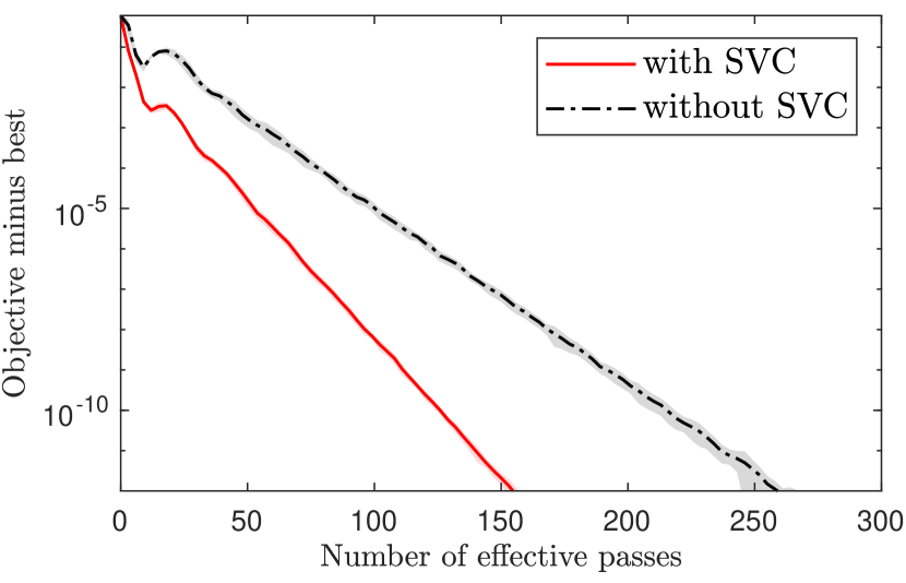
(a) Synthetic

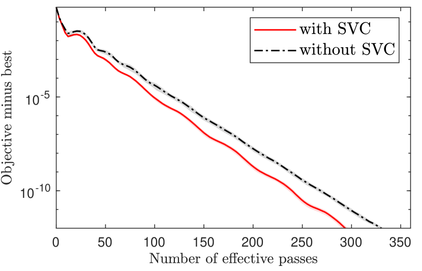
(b) KDD2010.small

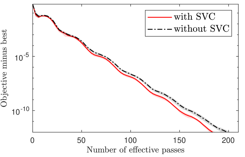
(c) RCV1.train

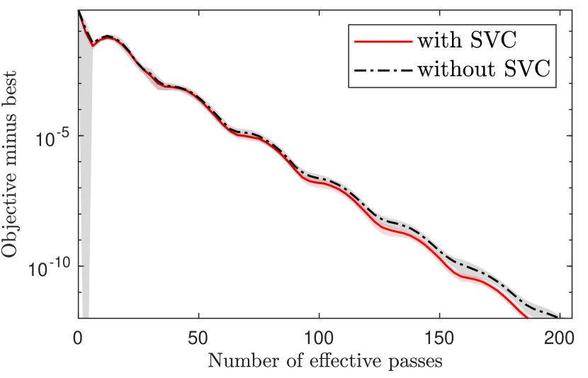
(d) News20

Figure 1: Ablation study for the practical effect of sparse variance correction (abbreviated as SVC in the legends). Run 10 seeds. Shaded bands indicate $\pm 1$ standard deviation.

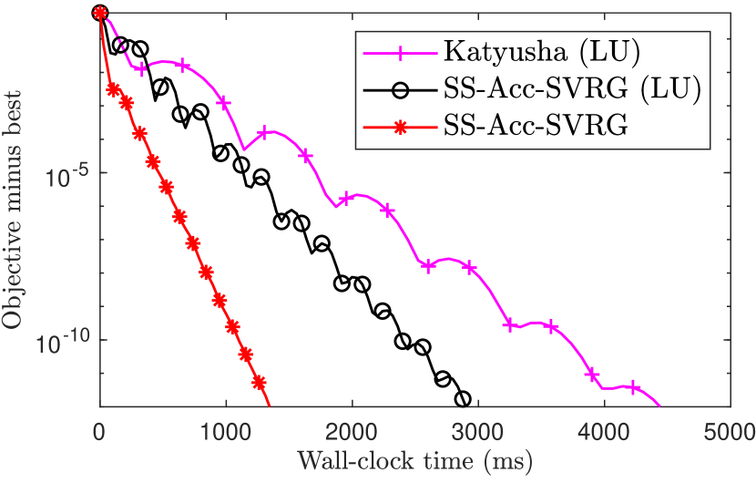
(a) Synthetic

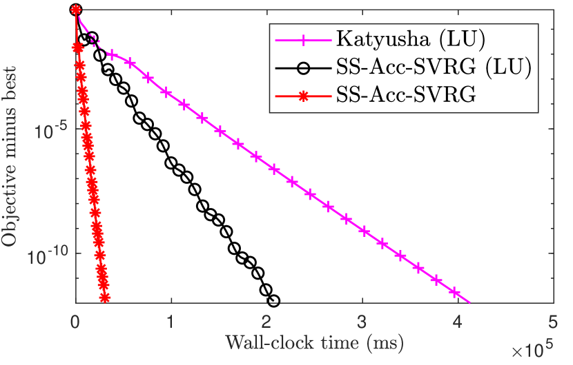
(b) KDD2010.small

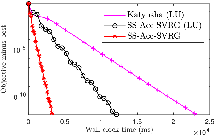
(c) RCV1.train

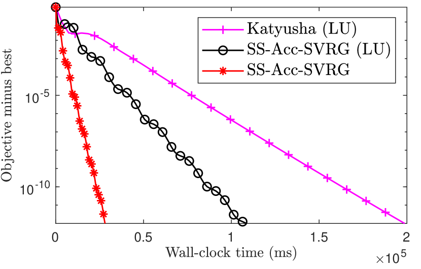
(d) News20

Figure 2: Running time comparison between using sparse gradient estimator and lagged update (abbreviated as LU in the legends). The wall-clock time and objective value are averaged over 10 runs.

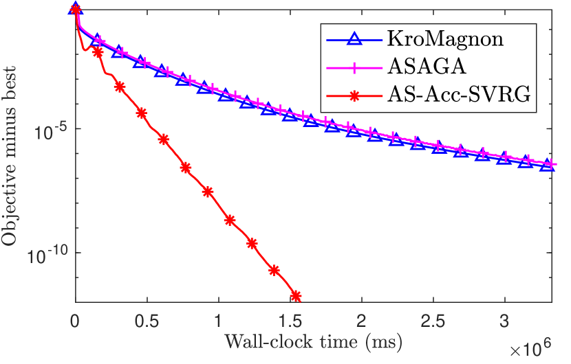
(a) KDD2010, $20$ threads

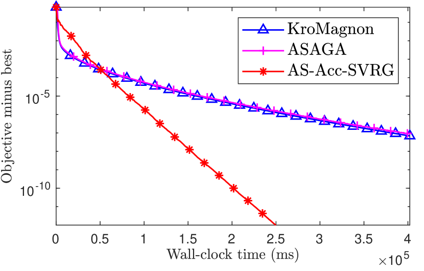
(b) RCV1.full, $20$ threads

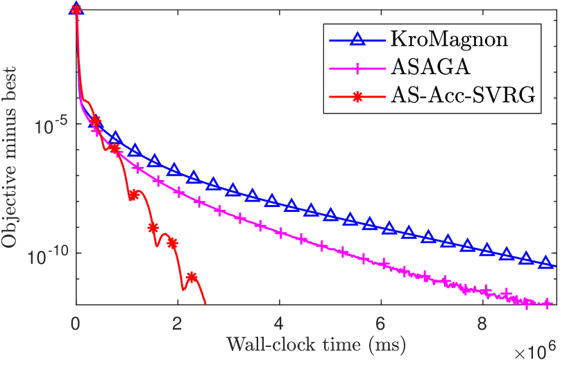
(c) Avazu-site.train, $20$ threads

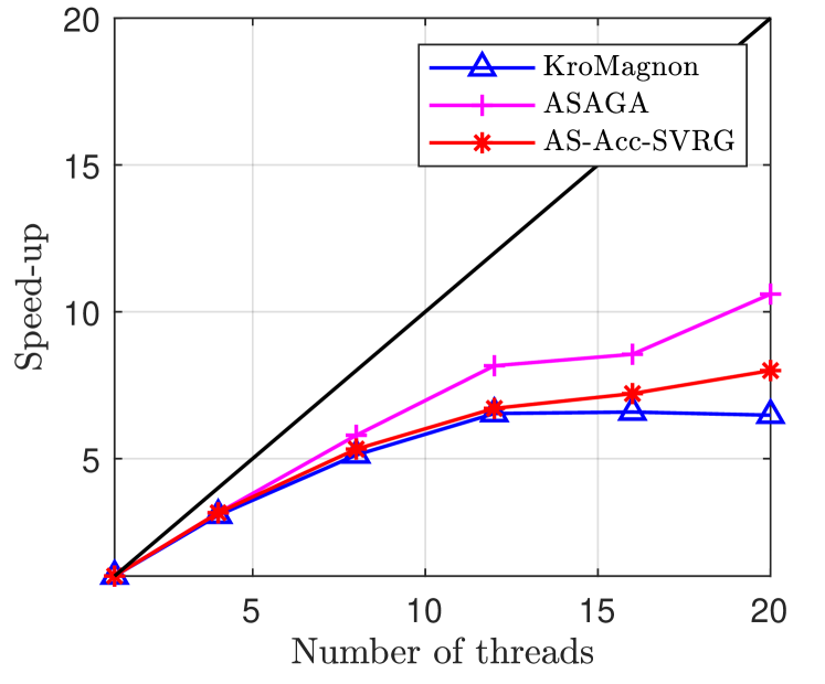
(d) KDD2010, speed-up

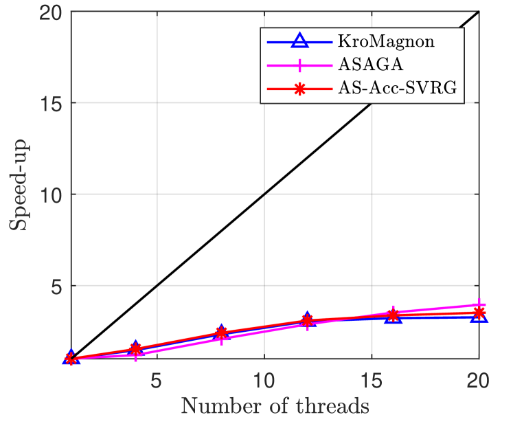
(e) RCV1.full, speed-up

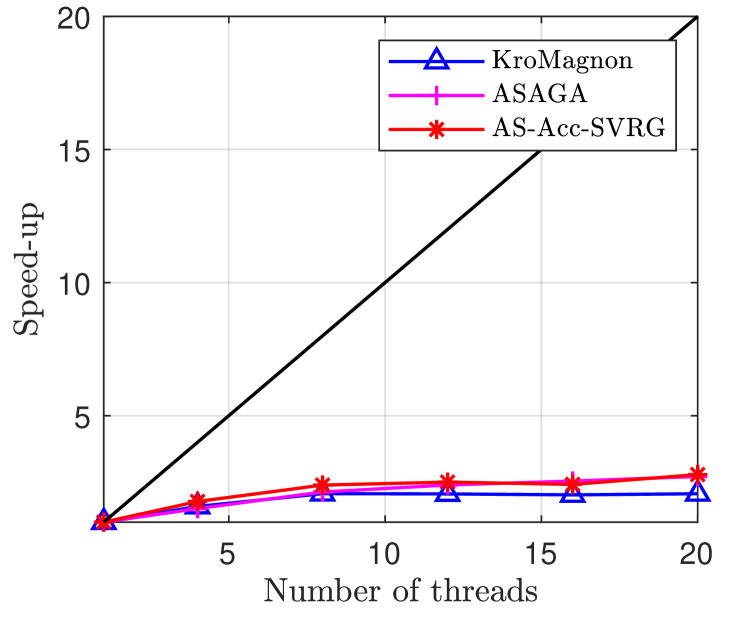
(f) Avazu-site.train, speed-up

Figure 3: Convergence and speed-up for asynchronous sparse methods. Speed-up is the improvement on the wall-clock time to achieve $10^{-5}$ sub-optimality relative to using a single thread.

5.3 Asynchronous Experiments

We compare the practical convergence and speed-up of AS-Acc-SVRG (Algorithm 2) with KroMagnon and ASAGA in Figure 3. We do not compare with the empirical method MiG in (Zhou et al.,, 2018), which requires us to tune two highly correlated parameters with only limited insights. This is expensive or even prohibited for large scale tasks. For the compared methods, we only tune the $\tau$-related constants in their theoretical parameter settings. That is, we tune the constant $1+2\sqrt{\Delta}\tilde{\tau}$ in Theorem 2 for AS-Acc-SVRG and the constant $c$ in the step size $\frac{1}{cL}$ for KroMagnon and ASAGA. In fact, in all the experiments, we simply fixed the constant to $1$ for AS-Acc-SVRG (the same parameters as the serial case), which worked smoothly. The main tuning effort was devoted to KroMagnon and ASAGA, and we tried to choose their step sizes as large as possible. The detailed choices can be found in Appendix G. Due to the scale of the problems, we only conducted a single run. From Figure 3, we see significant improvement of AS-Acc-SVRG for ill-conditioned tasks and similar practical speed-ups among the three methods, which verifies Theorem 2 and Corollary 2.1. We also observe a strong correlation between the practical speed-up and $\Delta$, which is predicted by the theoretical $O(1/\sqrt{\Delta})$ dependence. It seems that we cannot reproduce the speed-up results in (Leblond et al.,, 2018) on RCV1.full dataset. We believe that it is due to the usage of different programming languages, that we used a low-level heavily-optimized language C++ and they used high-level language Scalar. Pedregosa et al., (2017) also used C++ implementation and we observe a similar $10\times$ speed-up of ASAGA on KDD2010 dataset.

6 Conclusion

In this work, we proposed a new asynchronous accelerated SVRG method which achieves the optimal oracle complexity under the perturbed iterate framework. We show that it requires the same linear speed-up condition as the non-accelerated methods. Empirical results justified our findings.

A limitation of this work is that it does not support proximal operators, and we are currently not sure how to leverage the techniques in (Pedregosa et al.,, 2017) into our method. The main difficulty is on the choice of potential function.

Future directions could be (i) a more fine-grained analysis on $\Delta$ since currently $\Delta$ is a constant in all the datasets (except for the synthetic one), and (ii) designing asynchronous accelerated SAGA based on (Zhou et al.,, 2019) since SVRG variants still require at least one synchronization per epoch.

Appendix A Proof of Lemma 1

$$\mathbb{E}_{i}\left[\left\lVert\mathcal{G}_{y}-\nabla f(y)\right\rVert^{2}\right]$$

$$\overset{\mathclap{(a)}}{=}{} \mathbb{E}_{i}\left[\left\lVert\nabla f_{i}(y)-\nabla f_{i}(\tilde{x})+D_{i}\nabla f(\tilde{x})\right\rVert^{2}\right]-\left\lVert\nabla f(y)\right\rVert^{2}$$

$$={} \mathbb{E}_{i}\left[\left\lVert\nabla f_{i}(y)-\nabla f_{i}(\tilde{x})\right\rVert^{2}\right]+2\mathbb{E}_{i}\left[\left\langle\nabla f_{i}(y)-\nabla f_{i}(\tilde{x}),D_{i}\nabla f(\tilde{x})\right\rangle\right]+\mathbb{E}_{i}\left[\left\lVert D_{i}\nabla f(\tilde{x})\right\rVert^{2}\right]-\left\lVert\nabla f(y)\right\rVert^{2}$$

$$\overset{\mathclap{(b)}}{=}{} \mathbb{E}_{i}\left[\left\lVert\nabla f_{i}(y)-\nabla f_{i}(\tilde{x})\right\rVert^{2}\right]+2\mathbb{E}_{i}\left[\left\langle\nabla f_{i}(y)-\nabla f_{i}(\tilde{x}),D\nabla f(\tilde{x})\right\rangle\right]+\mathbb{E}_{i}\left[\left\langle D\nabla f(\tilde{x}),D_{i}\nabla f(\tilde{x})\right\rangle\right]-\left\lVert\nabla f(y)\right\rVert^{2}$$

$$={} \mathbb{E}_{i}\left[\left\lVert\nabla f_{i}(y)-\nabla f_{i}(\tilde{x})\right\rVert^{2}\right]+2\left\langle\nabla f(y),D\nabla f(\tilde{x})\right\rangle-\left\langle\nabla f(\tilde{x}),D\nabla f(\tilde{x})\right\rangle-\left\lVert\nabla f(y)\right\rVert^{2}$$

$$\overset{\mathclap{(c)}}{\leq}{} 2L\big{(}f(\tilde{x})-f(y)-\left\langle\nabla f(y),\tilde{x}-y\right\rangle\big{)}+2\left\langle\nabla f(y),D\nabla f(\tilde{x})\right\rangle-\left\langle\nabla f(\tilde{x}),D\nabla f(\tilde{x})\right\rangle-\left\lVert\nabla f(y)\right\rVert^{2},$$

where $\left(a\right)$ uses the unbiasedness $\mathbb{E}_{i}\left[\mathcal{G}_{y}\right]=\nabla f(y)$, $\left(b\right)$ follows from that $\nabla f_{i}(y)-\nabla f_{i}(\tilde{x})$ is supported on $T_{i}$ and $P_{i}^{2}=P_{i}$, and $\left(c\right)$ uses the interpolation condition of $f_{i}$ (see Section 2).

Appendix B Proof of Theorem 1

We omit the superscript $s$ in the one-epoch analysis for clarity. Using convexity, we have

$$f(y_{k})-f(x^{\star})\leq{} \left\langle\nabla f(y_{k}),y_{k}-x^{\star}\right\rangle$$

$$={} \left\langle\nabla f(y_{k}),y_{k}-z_{k}\right\rangle+\left\langle\nabla f(y_{k}),z_{k}-x^{\star}\right\rangle$$

$$\overset{\mathclap{(\star)}}{\leq}{} \frac{1-\vartheta}{\vartheta}\left\langle\nabla f(y_{k}),\tilde{x}_{s}-y_{k}\right\rangle-\frac{\varphi}{\vartheta}\left\langle\nabla f(y_{k}),D\nabla f(\tilde{x}_{s})\right\rangle+\left\langle\nabla f(y_{k}),z_{k}-x^{\star}\right\rangle,$$ (8)

where $\left(\star\right)$ follows from the construction $y_{k}=\vartheta z_{k}+\left(1-\vartheta\right)\tilde{x}_{s}-\varphi D\nabla f(\tilde{x}_{s})$.

Denote $\mathcal{G}_{y_{k}}=\nabla f_{i_{k}}(y_{k})-\nabla f_{i_{k}}(\tilde{x}_{s})+D_{i_{k}}\nabla f(\tilde{x}_{s})$. Based on the updating rule: $z_{k+1}=z_{k}-\eta\cdot\mathcal{G}_{y_{k}}$, it holds that

$$\left\lVert z_{k+1}-x^{\star}\right\rVert^{2}=\left\lVert z_{k}-x^{\star}-\eta\cdot\mathcal{G}_{y_{k}}\right\rVert^{2}$$

$$\Rightarrow{} \left\langle\mathcal{G}_{y_{k}},z_{k}-x^{\star}\right\rangle=\frac{\eta}{2}\left\lVert\mathcal{G}_{y_{k}}\right\rVert^{2}+\frac{1}{2\eta}\left(\left\lVert z_{k}-x^{\star}\right\rVert^{2}-\left\lVert z_{k+1}-x^{\star}\right\rVert^{2}\right)$$

$$\overset{\mathclap{(\star)}}{\Rightarrow}{} \left\langle\nabla f(y_{k}),z_{k}-x^{\star}\right\rangle=\frac{\eta}{2}\mathbb{E}_{i_{k}}\left[\left\lVert\mathcal{G}_{y_{k}}\right\rVert^{2}\right]+\frac{1}{2\eta}\left(\left\lVert z_{k}-x^{\star}\right\rVert^{2}-\mathbb{E}_{i_{k}}\left[\left\lVert z_{k+1}-x^{\star}\right\rVert^{2}\right]\right)$$

$$\Rightarrow{} \left\langle\nabla f(y_{k}),z_{k}-x^{\star}\right\rangle=\frac{\eta}{2}\mathbb{E}_{i_{k}}\left[\left\lVert\mathcal{G}_{y_{k}}-\nabla f(y_{k})\right\rVert^{2}\right]+\frac{\eta}{2}\left\lVert\nabla f(y_{k})\right\rVert^{2}+\frac{1}{2\eta}\left(\left\lVert z_{k}-x^{\star}\right\rVert^{2}-\mathbb{E}_{i_{k}}\left[\left\lVert z_{k+1}-x^{\star}\right\rVert^{2}\right]\right),$$ (9)

where $\left(\star\right)$ follows from taking the expectation with respect to sample $i_{k}$.

Combine (8), (9) and use the variance bound in Lemma 1.

$$f(y_{k})-f(x^{\star})\leq{} \eta L\big{(}f(\tilde{x}_{s})-f(y_{k})\big{)}+\left(\frac{1-\vartheta}{\vartheta}-\eta L\right)\left\langle\nabla f(y_{k}),\tilde{x}_{s}-y_{k}\right\rangle+\left(\eta-\frac{\varphi}{\vartheta}\right)\left\langle\nabla f(y_{k}),D\nabla f(\tilde{x}_{s})\right\rangle$$

$$-\frac{\eta}{2}\left\langle\nabla f(\tilde{x}_{s}),D\nabla f(\tilde{x}_{s})\right\rangle+\frac{1}{2\eta}\left(\left\lVert z_{k}-x^{\star}\right\rVert^{2}-\mathbb{E}_{i_{k}}\left[\left\lVert z_{k+1}-x^{\star}\right\rVert^{2}\right]\right).$$

Substituting the choices $\eta=\frac{1-\vartheta}{L\vartheta}$ and $\varphi=\eta\vartheta=\frac{1-\vartheta}{L}$ and noting that $D\succ 0$, we obtain

$$f(y_{k})-f(x^{\star})\leq{} (1-\vartheta)\big{(}f(\tilde{x}_{s})-f(x^{\star})\big{)}+\frac{L\vartheta^{2}}{2(1-\vartheta)}\left(\left\lVert z_{k}-x^{\star}\right\rVert^{2}-\mathbb{E}_{i_{k}}\left[\left\lVert z_{k+1}-x^{\star}\right\rVert^{2}\right]\right).$$

Summing the above inequality from $k=0$ to $m-1$ and noting that $z^{s+1}_{0}=z^{s}_{m}$, we obtain

$$\mathbb{E}\left[f(\tilde{x}_{s+1})-f(x^{\star})\right]={} \frac{1}{m}\sum_{k=0}^{m-1}{\mathbb{E}\left[f(y_{k})-f(x^{\star})\right]}$$

$$\leq{} (1-\vartheta)\mathbb{E}\left[f(\tilde{x}_{s})-f(x^{\star})\right]+\frac{L\vartheta^{2}}{2m(1-\vartheta)}\left(\mathbb{E}\left[\left\lVert z^{s}_{0}-x^{\star}\right\rVert^{2}\right]-\mathbb{E}\left[\left\lVert z^{s+1}_{0}-x^{\star}\right\rVert^{2}\right]\right).$$

Denoting $Q_{s}\triangleq\mathbb{E}\left[f(\tilde{x}_{s})-f(x^{\star})\right]$ and $P_{s}\triangleq\mathbb{E}\left[\left\lVert z^{s}_{0}-x^{\star}\right\rVert^{2}\right]$, we can write the above as

$$Q_{s+1}\leq{} \frac{1-\vartheta}{\vartheta}(Q_{s}-Q_{s+1})+\frac{L\vartheta}{2m(1-\vartheta)}\left(P_{s}-P_{s+1}\right).$$

Summing this inequality from $s=0$ to $S-1$ and using Jensen’s inequality, we have

$$\mathbb{E}\left[f(x_{r+1})-f(x^{\star})\right]\leq{} \frac{1}{S}\sum_{s=0}^{S-1}{Q_{s+1}}$$

$$\leq{} \frac{1-\vartheta}{\vartheta S}(Q_{0}-Q_{S})+\frac{L\vartheta}{2m(1-\vartheta)S}\left(P_{0}-P_{S}\right)$$

$$\overset{\mathclap{(\star)}}{\leq}{} \frac{1-\vartheta}{\vartheta S}\mathbb{E}\left[f(x_{r})-f(x^{\star})\right]+\frac{L\vartheta}{2m(1-\vartheta)S}\mathbb{E}\left[\left\lVert x_{r}-x^{\star}\right\rVert^{2}\right],$$

where $\left(\star\right)$ follows from $\tilde{x}_{0}=z^{0}_{0}=x_{r}$.

Using the $\mu$-strong convexity at $(x_{r},x^{\star})$ (or quadratic growth), i.e., $f(x_{r})-f(x^{\star})\geq\frac{\mu}{2}\left\lVert x_{r}-x^{\star}\right\rVert^{2}$, we arrive at

$$\mathbb{E}\left[f(x_{r+1})-f(x^{\star})\right]\leq\left(\frac{1-\vartheta}{\vartheta S}+\frac{\kappa\vartheta}{m(1-\vartheta)S}\right)\mathbb{E}\left[f(x_{r})-f(x^{\star})\right].$$

Choosing $S=\left\lceil\omega\cdot\left(\frac{1-\vartheta}{\vartheta}+\frac{\kappa\vartheta}{m(1-\vartheta)}\right)\right\rceil$, we have $\mathbb{E}\left[f(x_{r+1})-f(x^{\star})\right]\leq\frac{1}{\omega}\cdot\mathbb{E}\left[f(x_{r})-f(x^{\star})\right]$. Thus, for any accuracy $\epsilon>0$ and any constant $\omega>1$, to guarantee that the output satisfies $\mathbb{E}\left[f(x_{R})\right]-f(x^{\star})\leq\epsilon$, we need to perform totally $R=O\left(\log{\frac{f(x_{0})-f(x^{\star})}{\epsilon}}\right)$ restarts. Note that the total oracle complexity of Algorithm 1 is $\text{\#grad}=R\cdot S\cdot(n+2m)$. Setting $m=\Theta(n)$ and minimizing $S$ with respect to $\vartheta$, we obtain the optimal choice $\vartheta=\frac{\sqrt{m}}{\sqrt{\kappa}+\sqrt{m}}$. In this case, we have $S=\left\lceil 2\omega\sqrt{\frac{\kappa}{m}}\right\rceil=O\left(\max{\left\{1,\sqrt{\frac{\kappa}{n}}\right\}}\right)$. Finally, the total oracle complexity is

$$\text{\#grad}=O\left(\max{\left\{n,\sqrt{\kappa n}\right\}}\log{\frac{f(x_{0})-f(x^{\star})}{\epsilon}}\right).$$

Appendix C Proof of Theorem 2

We use the following lemma from (Leblond et al.,, 2018) to bound the term in asynchrony. Although the gradient is evaluated at a different point, the same proof works in our case, and thus is omitted here.

Lemma 2 (Inequality (63) in (Leblond et al.,, 2018)).

We have the following bound for the iterates $z_{k}$ (defined at (4)) and $\hat{z}_{k}$ (defined at (6)) in one epoch of Algorithm 2:

$$\mathbb{E}\left[\left\langle\mathcal{G}_{\hat{y}_{k}},\hat{z}_{k}-z_{k}\right\rangle\right]\leq\frac{\sqrt{\Delta}\eta}{2}\left(\sum_{j=(k-\tau)_{+}}^{k-1}{\mathbb{E}\left[\left\lVert\mathcal{G}_{\hat{y}_{j}}\right\rVert^{2}\right]+\tau\mathbb{E}\left[\left\lVert\mathcal{G}_{\hat{y}_{k}}\right\rVert^{2}\right]}\right).$$

We start with analyzing one epoch of virtual iterates defined at (4): $z_{k+1}=z_{k}-\eta\cdot\mathcal{G}_{\hat{y}_{k}}$. The expectation is first taken conditioned on the previous epochs.

$$\left\lVert z_{k+1}-x^{\star}\right\rVert^{2}=\left\lVert z_{k}-x^{\star}-\eta\cdot\mathcal{G}_{\hat{y}_{k}}\right\rVert^{2}$$

$$\Rightarrow{} \left\langle\mathcal{G}_{\hat{y}_{k}},\hat{z}_{k}-x^{\star}\right\rangle+\left\langle\mathcal{G}_{\hat{y}_{k}},z_{k}-\hat{z}_{k}\right\rangle=\frac{\eta}{2}\left\lVert\mathcal{G}_{\hat{y}_{k}}\right\rVert^{2}+\frac{1}{2\eta}\left(\left\lVert z_{k}-x^{\star}\right\rVert^{2}-\left\lVert z_{k+1}-x^{\star}\right\rVert^{2}\right)$$

$$\overset{\mathclap{(\star)}}{\Rightarrow}{} \mathbb{E}\left[\left\langle\nabla f(\hat{y}_{k}),\hat{z}_{k}-x^{\star}\right\rangle\right]=\frac{\eta}{2}\mathbb{E}\left[\left\lVert\mathcal{G}_{\hat{y}_{k}}\right\rVert^{2}\right]+\mathbb{E}\left[\left\langle\mathcal{G}_{\hat{y}_{k}},\hat{z}_{k}-z_{k}\right\rangle\right]+\frac{1}{2\eta}\left(\mathbb{E}\left[\left\lVert z_{k}-x^{\star}\right\rVert^{2}\right]-\mathbb{E}\left[\left\lVert z_{k+1}-x^{\star}\right\rVert^{2}\right]\right),$$ (10)

where $\left(\star\right)$ follows from taking the expectation and the unbiasedness assumption $\mathbb{E}\left[\mathcal{G}_{\hat{y}_{k}}|\hat{z}_{k}\right]=\nabla f(\hat{y}_{k})$.

Using the convexity at $x^{\star}$ and the inconsistent $\hat{y}_{k}$ (ordered at (5)), we have

$$f(\hat{y}_{k})-f(x^{\star})\leq{} \left\langle\nabla f(\hat{y}_{k}),\hat{y}_{k}-x^{\star}\right\rangle$$

$$={} \left\langle\nabla f(\hat{y}_{k}),\hat{y}_{k}-\hat{z}_{k}\right\rangle+\left\langle\nabla f(\hat{y}_{k}),\hat{z}_{k}-x^{\star}\right\rangle$$

$$\overset{\mathclap{(\star)}}{\leq}{} \frac{1-\vartheta}{\vartheta}\left\langle\nabla f(\hat{y}_{k}),\tilde{x}_{s}-\hat{y}_{k}\right\rangle-\frac{\varphi}{\vartheta}\left\langle\nabla f(\hat{y}_{k}),D\nabla f(\tilde{x}_{s})\right\rangle+\left\langle\nabla f(\hat{y}_{k}),\hat{z}_{k}-x^{\star}\right\rangle.$$

where $\left(\star\right)$ follows from the construction $\hat{y}_{k}=\vartheta\hat{z}_{k}+\left(1-\vartheta\right)\tilde{x}_{s}-\varphi D\nabla f(\tilde{x}_{s})$.

After taking the expectation and combining with (10), we obtain

$$\mathbb{E}\left[f(\hat{y}_{k})\right]-f(x^{\star})\leq{} \frac{1-\vartheta}{\vartheta}\mathbb{E}\left[\left\langle\nabla f(\hat{y}_{k}),\tilde{x}_{s}-\hat{y}_{k}\right\rangle\right]-\frac{\varphi}{\vartheta}\mathbb{E}\left[\left\langle\nabla f(\hat{y}_{k}),D\nabla f(\tilde{x}_{s})\right\rangle\right]+\frac{\eta}{2}\mathbb{E}\left[\left\lVert\mathcal{G}_{\hat{y}_{k}}\right\rVert^{2}\right]$$

$$+\mathbb{E}\left[\left\langle\mathcal{G}_{\hat{y}_{k}},\hat{z}_{k}-z_{k}\right\rangle\right]+\frac{1}{2\eta}\left(\mathbb{E}\left[\left\lVert z_{k}-x^{\star}\right\rVert^{2}\right]-\mathbb{E}\left[\left\lVert z_{k+1}-x^{\star}\right\rVert^{2}\right]\right).$$

Summing this inequality from $k=0$ to $m-1$, we have

$$\sum_{k=0}^{m-1}{\mathbb{E}\left[f(\hat{y}_{k})-f(x^{\star})\right]}\leq{} \sum_{k=0}^{m-1}{\left(\frac{1-\vartheta}{\vartheta}\mathbb{E}\left[\left\langle\nabla f(\hat{y}_{k}),\tilde{x}_{s}-\hat{y}_{k}\right\rangle\right]-\frac{\varphi}{\vartheta}\mathbb{E}\left[\left\langle\nabla f(\hat{y}_{k}),D\nabla f(\tilde{x}_{s})\right\rangle\right]+\frac{\eta}{2}\mathbb{E}\left[\left\lVert\mathcal{G}_{\hat{y}_{k}}\right\rVert^{2}\right]\right)}$$

$$+\sum_{k=0}^{m-1}{\mathbb{E}\left[\left\langle\mathcal{G}_{\hat{y}_{k}},\hat{z}_{k}-z_{k}\right\rangle\right]}+\frac{1}{2\eta}\left(\left\lVert z_{0}-x^{\star}\right\rVert^{2}-\mathbb{E}\left[\left\lVert z_{m}-x^{\star}\right\rVert^{2}\right]\right).$$

Invoke Lemma 2 to bound the asynchronous perturbation.

$$\sum_{k=0}^{m-1}{\mathbb{E}\left[f(\hat{y}_{k})-f(x^{\star})\right]}$$

$$\leq{} \sum_{k=0}^{m-1}{\left(\frac{1-\vartheta}{\vartheta}\mathbb{E}\left[\left\langle\nabla f(\hat{y}_{k}),\tilde{x}_{s}-\hat{y}_{k}\right\rangle\right]-\frac{\varphi}{\vartheta}\mathbb{E}\left[\left\langle\nabla f(\hat{y}_{k}),D\nabla f(\tilde{x}_{s})\right\rangle\right]+\frac{\eta}{2}\mathbb{E}\left[\left\lVert\mathcal{G}_{\hat{y}_{k}}\right\rVert^{2}\right]\right)}$$

$$+\frac{\sqrt{\Delta}\eta}{2}\sum_{k=0}^{m-1}{\left(\sum_{j=(k-\tau)_{+}}^{k-1}{\mathbb{E}\left[\left\lVert\mathcal{G}_{\hat{y}_{j}}\right\rVert^{2}\right]+\tau\mathbb{E}\left[\left\lVert\mathcal{G}_{\hat{y}_{k}}\right\rVert^{2}\right]}\right)}+\frac{1}{2\eta}\left(\left\lVert z_{0}-x^{\star}\right\rVert^{2}-\mathbb{E}\left[\left\lVert z_{m}-x^{\star}\right\rVert^{2}\right]\right)$$

$$={} \sum_{k=0}^{m-1}{\left(\frac{1-\vartheta}{\vartheta}\mathbb{E}\left[\left\langle\nabla f(\hat{y}_{k}),\tilde{x}_{s}-\hat{y}_{k}\right\rangle\right]-\frac{\varphi}{\vartheta}\mathbb{E}\left[\left\langle\nabla f(\hat{y}_{k}),D\nabla f(\tilde{x}_{s})\right\rangle\right]+\frac{\eta(1+\sqrt{\Delta}\tau)}{2}\mathbb{E}\left[\left\lVert\mathcal{G}_{\hat{y}_{k}}\right\rVert^{2}\right]\right)}$$

$$+\frac{\sqrt{\Delta}\eta}{2}\sum_{k=0}^{m-1}{\sum_{j=(k-\tau)_{+}}^{k-1}{\mathbb{E}\left[\left\lVert\mathcal{G}_{\hat{y}_{j}}\right\rVert^{2}\right]}}+\frac{1}{2\eta}\left(\left\lVert z_{0}-x^{\star}\right\rVert^{2}-\mathbb{E}\left[\left\lVert z_{m}-x^{\star}\right\rVert^{2}\right]\right)$$

$$\leq{} \sum_{k=0}^{m-1}{\left(\frac{1-\vartheta}{\vartheta}\mathbb{E}\left[\left\langle\nabla f(\hat{y}_{k}),\tilde{x}_{s}-\hat{y}_{k}\right\rangle\right]-\frac{\varphi}{\vartheta}\mathbb{E}\left[\left\langle\nabla f(\hat{y}_{k}),D\nabla f(\tilde{x}_{s})\right\rangle\right]+\frac{\eta(1+\sqrt{\Delta}\tau)}{2}\mathbb{E}\left[\left\lVert\mathcal{G}_{\hat{y}_{k}}\right\rVert^{2}\right]\right)}$$

$$+\frac{\sqrt{\Delta}\eta\tau}{2}\sum_{k=0}^{m-1}{\mathbb{E}\left[\left\lVert\mathcal{G}_{\hat{y}_{k}}\right\rVert^{2}\right]}+\frac{1}{2\eta}\left(\left\lVert z_{0}-x^{\star}\right\rVert^{2}-\mathbb{E}\left[\left\lVert z_{m}-x^{\star}\right\rVert^{2}\right]\right)$$

$$={} \sum_{k=0}^{m-1}{\left(\frac{1-\vartheta}{\vartheta}\mathbb{E}\left[\left\langle\nabla f(\hat{y}_{k}),\tilde{x}_{s}-\hat{y}_{k}\right\rangle\right]-\frac{\varphi}{\vartheta}\mathbb{E}\left[\left\langle\nabla f(\hat{y}_{k}),D\nabla f(\tilde{x}_{s})\right\rangle\right]+\frac{\eta(1+2\sqrt{\Delta}\tau)}{2}\mathbb{E}\left[\left\lVert\mathcal{G}_{\hat{y}_{k}}\right\rVert^{2}\right]\right)}$$

$$+\frac{1}{2\eta}\left(\left\lVert z_{0}-x^{\star}\right\rVert^{2}-\mathbb{E}\left[\left\lVert z_{m}-x^{\star}\right\rVert^{2}\right]\right).$$

For some $\widetilde{\tau}\geq\tau$, we choose $\eta=\frac{(1-\vartheta)}{L\vartheta(1+2\sqrt{\Delta}\widetilde{\tau})}$, and then

$$\sum_{k=0}^{m-1}{\mathbb{E}\left[f(\hat{y}_{k})-f(x^{\star})\right]}\leq{} \sum_{k=0}^{m-1}{\left(\frac{1-\vartheta}{\vartheta}\mathbb{E}\left[\left\langle\nabla f(\hat{y}_{k}),\tilde{x}_{s}-\hat{y}_{k}\right\rangle\right]-\frac{\varphi}{\vartheta}\mathbb{E}\left[\left\langle\nabla f(\hat{y}_{k}),D\nabla f(\tilde{x}_{s})\right\rangle\right]+\frac{1-\vartheta}{2L\vartheta}\mathbb{E}\left[\left\lVert\mathcal{G}_{\hat{y}_{k}}\right\rVert^{2}\right]\right)}$$

$$+\frac{L\vartheta(1+2\sqrt{\Delta}\widetilde{\tau})}{2(1-\vartheta)}\left(\left\lVert z_{0}-x^{\star}\right\rVert^{2}-\mathbb{E}\left[\left\lVert z_{m}-x^{\star}\right\rVert^{2}\right]\right).$$

Note that $\mathbb{E}\left[\left\lVert\mathcal{G}_{\hat{y}_{k}}\right\rVert^{2}\right]=\mathbb{E}\left[\left\lVert\mathcal{G}_{\hat{y}_{k}}-\nabla f(\hat{y}_{k})\right\rVert^{2}\right]+\mathbb{E}\left[\left\lVert\nabla f(\hat{y}_{k})\right\rVert^{2}\right]$ due to the unbiasedness assumption. Using Lemma 1, we can conclude that

$$\sum_{k=0}^{m-1}{\mathbb{E}\left[f(\hat{y}_{k})-f(x^{\star})\right]}\leq{} \sum_{k=0}^{m-1}{\left(\left(\frac{1-\vartheta}{L\vartheta}-\frac{\varphi}{\vartheta}\right)\mathbb{E}\left[\left\langle\nabla f(\hat{y}_{k}),D\nabla f(\tilde{x}_{s})\right\rangle\right]+\frac{1-\vartheta}{\vartheta}\big{(}f(\tilde{x}_{s})-\mathbb{E}\left[f(\hat{y}_{k})\right]\big{)}\right)}$$

$$+\frac{L\vartheta(1+2\sqrt{\Delta}\widetilde{\tau})}{2(1-\vartheta)}\left(\left\lVert z_{0}-x^{\star}\right\rVert^{2}-\mathbb{E}\left[\left\lVert z_{m}-x^{\star}\right\rVert^{2}\right]\right).$$

Choosing $\varphi=\frac{1-\vartheta}{L}$ and dividing both sides by $m$, we can arrange this inequality as

$$\frac{1}{m}\sum_{k=0}^{m-1}{\mathbb{E}\left[f(\hat{y}_{k})-f(x^{\star})\right]}\leq(1-\vartheta)\big{(}f(\tilde{x}_{s})-f(x^{\star})\big{)}+\frac{L\vartheta^{2}(1+2\sqrt{\Delta}\widetilde{\tau})}{2m(1-\vartheta)}\left(\left\lVert z_{0}-x^{\star}\right\rVert^{2}-\mathbb{E}\left[\left\lVert z_{m}-x^{\star}\right\rVert^{2}\right]\right).$$

Since $\tilde{x}_{s+1}$ is chosen uniformly at random from $\{\hat{y}_{0},\ldots,\hat{y}_{m-1}\}$ and that $z^{s+1}_{0}=z^{s}_{m}$ (the first and the last virtual iterates exist in the shared memory, and $z$ is unchanged after each epoch in Algorithm 2), the following holds

$$\begin{gathered}\mathbb{E}\left[f(\tilde{x}_{s+1})-f(x^{\star})\right]\leq(1-\vartheta)\big{(}f(\tilde{x}_{s})-f(x^{\star})\big{)}+\frac{L\vartheta^{2}(1+2\sqrt{\Delta}\widetilde{\tau})}{2m(1-\vartheta)}\left(\left\lVert z^{s}_{0}-x^{\star}\right\rVert^{2}-\mathbb{E}\left[\left\lVert z^{s+1}_{0}-x^{\star}\right\rVert^{2}\right]\right).\end{gathered}$$

For the sake of clarity, we denote $Q_{s}\triangleq\mathbb{E}\left[f(\tilde{x}_{s})-f(x^{\star})\right]$ and $P_{s}\triangleq\mathbb{E}\left[\left\lVert z^{s}_{0}-x^{\star}\right\rVert^{2}\right]$. Then, it holds that

$$Q_{s+1}\leq\frac{1-\vartheta}{\vartheta}(Q_{s}-Q_{s+1})+\frac{L\vartheta(1+2\sqrt{\Delta}\widetilde{\tau})}{2m(1-\vartheta)}\left(P_{s}-P_{s+1}\right).$$

Summing this inequality from $s=0$ to $S-1$ and using Jensen’s inequality, we have

$$\mathbb{E}\left[f(x_{r+1})\right]-f(x^{\star})\leq{} \frac{1}{S}\sum_{s=0}^{S-1}{Q_{s+1}}$$

$$\leq{} \frac{1-\vartheta}{\vartheta S}(Q_{0}-Q_{S})+\frac{L\vartheta(1+2\sqrt{\Delta}\widetilde{\tau})}{2m(1-\vartheta)S}\left(P_{0}-P_{S}\right)$$

$$\leq{} \frac{1-\vartheta}{\vartheta S}Q_{0}+\frac{L\vartheta(1+2\sqrt{\Delta}\widetilde{\tau})}{2m(1-\vartheta)S}P_{0}.$$

Using $\mu$-strong convexity at $(x_{r},x^{\star})$ (or quadratic growth), we have $\left\lVert x_{r}-x^{\star}\right\rVert^{2}\leq\frac{2}{\mu}\big{(}f(x_{r})-f(x^{\star})\big{)}\Leftrightarrow P_{0}\leq\frac{2}{\mu}Q_{0}$ and thus

$$\mathbb{E}\left[f(x_{r+1})\right]-f(x^{\star})\leq\left(\frac{1-\vartheta}{\vartheta S}+\frac{\kappa\vartheta(1+2\sqrt{\Delta}\widetilde{\tau})}{m(1-\vartheta)S}\right)\mathbb{E}\left[f(x_{r})-f(x^{\star})\right],$$

Letting $S=\left\lceil\omega\cdot\left(\frac{1-\vartheta}{\vartheta}+\frac{\kappa\vartheta(1+2\sqrt{\Delta}\widetilde{\tau})}{m(1-\vartheta)}\right)\right\rceil$, we have $\mathbb{E}\left[f(x_{r+1})\right]-f(x^{\star})\leq\frac{1}{\omega}\cdot\mathbb{E}\left[f(x_{r})-f(x^{\star})\right]$. Then, since $\omega>1$ is a constant, to achieve an $\epsilon$-additive error, we need to restart totally $R=O\left(\log{\frac{f(x_{0})-f(x^{\star})}{\epsilon}}\right)$ times. Note that the total oracle complexity of Algorithm 2 is $\text{\#grad}=R\cdot S\cdot(n+2m)$. Setting $m=\Theta(n)$ and choosing $\vartheta$ that minimizes $S$, we obtain the optimal choice $\vartheta=\frac{\sqrt{m}}{\sqrt{\kappa(1+2\sqrt{\Delta}\widetilde{\tau})}+\sqrt{m}}$, which leads to $S=\left\lceil 2\omega\sqrt{\frac{\kappa}{m}(1+2\sqrt{\Delta}\widetilde{\tau})}\right\rceil=O\left(\max{\left\{1,\sqrt{\frac{\kappa}{n}(1+2\sqrt{\Delta}\widetilde{\tau})}\right\}}\right)$. Finally, the total oracle complexity is

$$\text{\#grad}=O\left(\max{\left\{n,\sqrt{\kappa n(1+2\sqrt{\Delta}\widetilde{\tau})}\right\}}\log{\frac{f(x_{0})-f(x^{\star})}{\epsilon}}\right).$$

Appendix D The Effect of the Constant $\omega$ (the Restart Frequency)

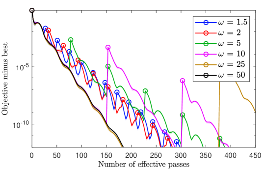
Figure 4: The practical effect of $\omega$. RCV1.train, run $10$ seeds. The circle marks the restarting points, i.e., $\{x_{r}\}$. Shaded bands indicate $\pm 1$ standard deviation.

We numerically evaluate the effect of the constant $\omega$ in Figure 4. We choose $\omega$ from $1.5$ (frequent restart) to $50$ (not restart in this task). The results on News20 and KDD2010.small datasets are basically identical, and thus are omitted here. As we can see, unfortunately, the restarts only deteriorate the performance. An intuitive explanation is that the restart strategy is more conservative as it periodically retracts the point. In theory, the explicit dependence on $\omega$ (in the serial case) is

$$\frac{1}{\log{\omega}}\left\lceil 2\omega\sqrt{\frac{\kappa}{m}}\right\rceil,$$

which suggests that if $\omega$ is large, the convergence on the restarting points $\{x_{r}\}$ will be slower. This is observed in Figure 4. However, what our current theory cannot explain is the superior performance of not performing restart, and we are not aware a situation where the “aggressiveness” of no restart would hurt the convergence. Optimally tuning $\omega$ in the complexity will only leads to a small $\omega$ that closes to $1$. Further investigation is needed for the convergence of Algorithms 1 and 2 without restart (we have strong numerical evidence in Appendix E that without restart, they are still optimal).

Appendix E Justifying the $\sqrt{\kappa}$ Dependence

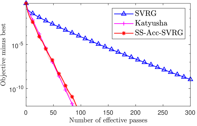
(a) KDD2010.small, $\mu=10^{-6}$.

(b) RCV1.train, $\mu=10^{-5}$.

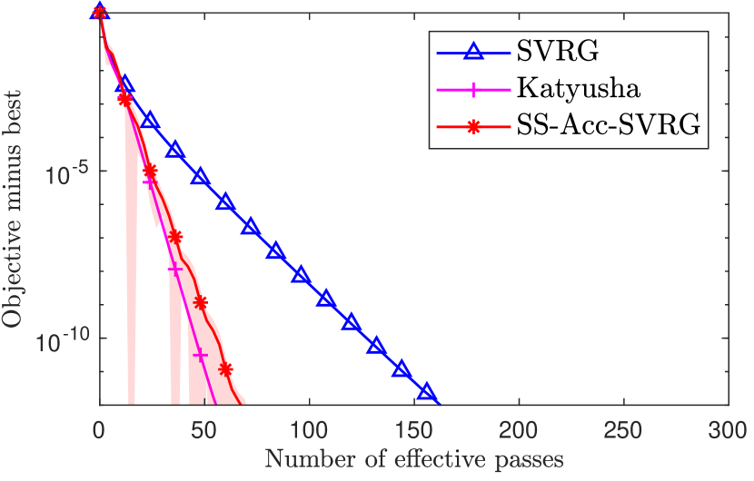
(c) News20, $\mu=10^{-5}$.

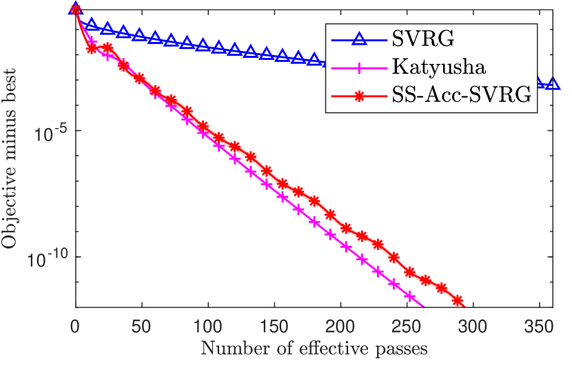
(d) KDD2010.small, $\mu=10^{-7}$.

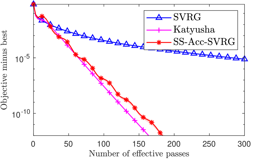
(e) RCV1.train, $\mu=10^{-6}$.

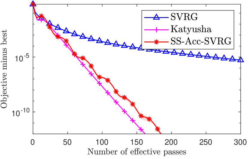
(f) News20, $\mu=10^{-6}$.

Figure 5: Justifying the $\sqrt{\kappa}$ dependence. Run $10$ seeds. Shaded bands indicate $\pm 1$ standard deviation.

We choose $\mu$ to be $10$-times larger (Figure 5(a) to 5(c)) than the ones specified in Table 1 (Figure 5(d) to 5(f)) to verify the $\sqrt{\kappa}$ dependence. In this case, $\kappa$ is $10$-times smaller and we expect the accelerated methods to be around $3$-times faster in terms of the number of data passes. This has been observed across all the datasets for Katyusha and SS-Acc-SVRG, which verifies the accelerated rate.

Appendix F Sanity Check for Our Implementation

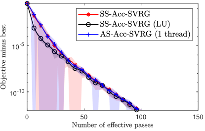
Figure 6: Sanity check. a9a.dense, $\mu=10^{-6}$. Run $20$ seeds. Shaded bands indicate $\pm 1$ standard deviation.

If the dataset is fully dense, then the following three schemes should be equivalent: SS-Acc-SVRG, SS-Acc-SVRG with lagged update implementation and AS-Acc-SVRG with a single thread. We construct a fully dense dataset by adding a small positive number to each elements in a9a dataset (Chang and Lin,, 2011) ($n=$32,561\text{\,}$,d=123$), and we call it a9a.dense dataset. The sanity check is then provided in Figure 6. SS-Acc-SVRG (LU) shows slightly different convergence because we used an averaged snapshot instead of a random one in its implementation. Implementing lagged update technique with a random snapshot is quite tricky, since the last seen iteration might be in the previous epochs in this case. We tested SS-Acc-SVRG with an averaged snapshot and it shows almost identical convergence as SS-Acc-SVRG (LU).

Appendix G Experimental Setup

All the methods are implemented in C++.

Serial setup

We ran serial experiments on an HP Z440 machine with a single Intel Xeon E5-1630v4 with 3.70GHz cores, 16GB RAM, Ubuntu 18.04 LTS with GCC 9.4.0, MATLAB R2021a. We fixed the epoch length $m=2n$ and chose the default parameters: SS-Acc-SVRG follows Theorem 1; Katyusha uses $\tau_{2}=\frac{1}{2},\tau_{1}=\sqrt{\frac{m}{3\kappa}},\alpha=\frac{1}{3\tau_{1}L}$ (Allen-Zhu,, 2017); SVRG uses $\eta=\frac{1}{4L}$.

Asynchronous setup

We ran asynchronous experiments on a Dell PowerEdge R840 HPC with four Intel Xeon Platinum 8160 CPU @ 2.10GHz each with 24 cores, 768GB RAM, CentOS 7.9.2009 with GCC 9.3.1, MATLAB R2021a. We implemented the original version of KroMagnon in (Mania et al.,, 2017). We fixed the epoch length $m=2n$ for KroMagnon and AS-Acc-SVRG. AS-Acc-SVRG used the same parameters as in the serial case for all datasets. The step sizes of KroMagnon and ASAGA were chosen as follows: On RCV1.full, KroMagnon uses $\frac{1}{L}$, ASAGA uses $\frac{1}{1.3L}$; On Avazu-site.train, KroMagnon uses $\frac{1}{2L}$, ASAGA uses $\frac{1}{2L}$; On KDD2010, KroMagnon uses $\frac{1}{2L}$, ASAGA uses $\frac{1}{3L}$. Due to the scale of the tasks, we cannot do fine-grained grid search for the step sizes of KroMagnon and ASAGA. They were chosen to ensure a stable and consistent performance in the 20-thread experiments.

References

- Allen-Zhu, (2017) Allen-Zhu, Z. (2017). Katyusha: The First Direct Acceleration of Stochastic Gradient Methods. Journal of Machine Learning Research, 18(1):8194–8244.
- Chang and Lin, (2011) Chang, C.-C. and Lin, C.-J. (2011). LIBSVM: A library for support vector machines. ACM Transactions on Intelligent Systems and Technology, 2:27:1–27:27. Software available at http://www.csie.ntu.edu.tw/~cjlin/libsvm.
- Cyrus et al., (2018) Cyrus, S., Hu, B., Van Scoy, B., and Lessard, L. (2018). A robust accelerated optimization algorithm for strongly convex functions. In Annual American Control Conference (ACC), pages 1376–1381. IEEE.
- Defazio et al., (2014) Defazio, A., Bach, F. R., and Lacoste-Julien, S. (2014). SAGA: A Fast Incremental Gradient Method With Support for Non-Strongly Convex Composite Objectives. In Advances in Neural Information Processing Systems, pages 1646–1654.
- Devolder et al., (2014) Devolder, O., Glineur, F., and Nesterov, Y. (2014). First-order methods of smooth convex optimization with inexact oracle. Mathematical Programming, 146(1):37–75.
- Dubois-Taine et al., (2021) Dubois-Taine, B., Vaswani, S., Babanezhad, R., Schmidt, M., and Lacoste-Julien, S. (2021). SVRG Meets AdaGrad: Painless Variance Reduction. arXiv preprint arXiv:2102.09645.
- Duchi et al., (2013) Duchi, J. C., Jordan, M. I., and McMahan, H. B. (2013). Estimation, Optimization, and Parallelism when Data is Sparse. In Advances in Neural Information Processing Systems, pages 2832–2840.
- Fang et al., (2018) Fang, C., Huang, Y., and Lin, Z. (2018). Accelerating asynchronous algorithms for convex optimization by momentum compensation. arXiv preprint arXiv:1802.09747.
- Gu et al., (2020) Gu, B., Xian, W., Huo, Z., Deng, C., and Huang, H. (2020). A Unified q-Memorization Framework for Asynchronous Stochastic Optimization. Journal of Machine Learning Research, 21:190–1.
- Hannah et al., (2019) Hannah, R., Feng, F., and Yin, W. (2019). A2BCD: Asynchronous Acceleration with Optimal Complexity. In International Conference on Learning Representations.
- Hofmann et al., (2015) Hofmann, T., Lucchi, A., Lacoste-Julien, S., and McWilliams, B. (2015). Variance Reduced Stochastic Gradient Descent with Neighbors. In Advances in Neural Information Processing Systems, pages 2305–2313.
- Johnson and Zhang, (2013) Johnson, R. and Zhang, T. (2013). Accelerating Stochastic Gradient Descent using Predictive Variance Reduction. In Advances in Neural Information Processing Systems, pages 315–323.
- Joulani et al., (2019) Joulani, P., György, A., and Szepesvári, C. (2019). Think out of the ”Box”: Generically-Constrained Asynchronous Composite Optimization and Hedging. In Advances in Neural Information Processing Systems, pages 12225–12235.
- Juan et al., (2016) Juan, Y., Zhuang, Y., Chin, W., and Lin, C. (2016). Field-aware Factorization Machines for CTR Prediction. In Proceedings of the 10th ACM Conference on Recommender Systems, pages 43–50. ACM.
- Karimi et al., (2016) Karimi, H., Nutini, J., and Schmidt, M. (2016). Linear Convergence of Gradient and Proximal-Gradient Methods Under the Polyak-Łojasiewicz Condition. In Joint European Conference on Machine Learning and Knowledge Discovery in Databases, pages 795–811. Springer.
- Keerthi et al., (2005) Keerthi, S. S., DeCoste, D., and Joachims, T. (2005). A Modified Finite Newton Method for Fast Solution of Large Scale Linear SVMs. Journal of Machine Learning Research, 6:341–361.
- Konečnỳ and Richtárik, (2013) Konečnỳ, J. and Richtárik, P. (2013). Semi-stochastic gradient descent methods. arXiv preprint arXiv:1312.1666.
- Lan et al., (2019) Lan, G., Li, Z., and Zhou, Y. (2019). A unified variance-reduced accelerated gradient method for convex optimization. In Advances in Neural Information Processing Systems, volume 32, pages 10462–10472.
- Leblond et al., (2017) Leblond, R., Pedregosa, F., and Lacoste-Julien, S. (2017). ASAGA: Asynchronous Parallel SAGA. In Proceedings of the Twentieth International Conference on Artificial Intelligence and Statistics, volume 54, pages 46–54.
- Leblond et al., (2018) Leblond, R., Pedregosa, F., and Lacoste-Julien, S. (2018). Improved Asynchronous Parallel Optimization Analysis for Stochastic Incremental Methods. Journal of Machine Learning Research, 19:81:1–81:68.
- Lewis et al., (2004) Lewis, D. D., Yang, Y., Russell-Rose, T., and Li, F. (2004). RCV1: A New Benchmark Collection for Text Categorization Research. Journal of Machine Learning Research, 5:361–397.
- Li, (2021) Li, Z. (2021). ANITA: An Optimal Loopless Accelerated Variance-Reduced Gradient Method. arXiv preprint arXiv:2103.11333.
- Lian et al., (2015) Lian, X., Huang, Y., Li, Y., and Liu, J. (2015). Asynchronous Parallel Stochastic Gradient for Nonconvex Optimization. In Advances in Neural Information Processing Systems, pages 2737–2745.
- Mania et al., (2017) Mania, H., Pan, X., Papailiopoulos, D. S., Recht, B., Ramchandran, K., and Jordan, M. I. (2017). Perturbed Iterate Analysis for Asynchronous Stochastic Optimization. SIAM Journal on Optimization, 27(4):2202–2229.
- Nesterov, (1983) Nesterov, Y. (1983). A method for solving the convex programming problem with convergence rate . In Dokl. akad. nauk Sssr, volume 269, pages 543–547.
- Nesterov, (2003) Nesterov, Y. (2003). Introductory lectures on convex optimization: A basic course, volume 87. Springer Science & Business Media.
- Nesterov, (2005) Nesterov, Y. (2005). Smooth minimization of non-smooth functions. Mathematical Programming, 103(1):127–152.
- Nesterov, (2018) Nesterov, Y. (2018). Lectures on convex optimization, volume 137. Springer.
- Nguyen et al., (2017) Nguyen, L. M., Liu, J., Scheinberg, K., and Takáč, M. (2017). SARAH: A Novel Method for Machine Learning Problems Using Stochastic Recursive Gradient. In Proceedings of the 34th International Conference on Machine Learning, pages 2613–2621.
- Nguyen et al., (2018) Nguyen, L. M., Nguyen, P. H., van Dijk, M., Richtárik, P., Scheinberg, K., and Takác, M. (2018). SGD and Hogwild! Convergence Without the Bounded Gradients Assumption. In Proceedings of the 35th International Conference on Machine Learning, volume 80, pages 3747–3755.
- Pedregosa et al., (2017) Pedregosa, F., Leblond, R., and Lacoste-Julien, S. (2017). Breaking the Nonsmooth Barrier: A Scalable Parallel Method for Composite Optimization. In Advances in Neural Information Processing Systems, pages 56–65.
- Recht et al., (2011) Recht, B., Ré, C., Wright, S. J., and Niu, F. (2011). Hogwild!: A Lock-Free Approach to Parallelizing Stochastic Gradient Descent. In Advances in Neural Information Processing Systems, pages 693–701.
- Roux et al., (2012) Roux, N. L., Schmidt, M., and Bach, F. R. (2012). A Stochastic Gradient Method with an Exponential Convergence Rate for Finite Training Sets. In Advances in Neural Information Processing Systems, pages 2663–2671.
- Sa et al., (2015) Sa, C. D., Zhang, C., Olukotun, K., and Ré, C. (2015). Taming the Wild: A Unified Analysis of Hogwild-Style Algorithms. In Advances in Neural Information Processing Systems, pages 2674–2682.
- Schmidt et al., (2017) Schmidt, M., Le Roux, N., and Bach, F. (2017). Minimizing finite sums with the stochastic average gradient. Mathematical Programming, 162(1-2):83–112.
- Shang et al., (2018) Shang, F., Liu, Y., Zhou, K., Cheng, J., Ng, K. K. W., and Yoshida, Y. (2018). Guaranteed Sufficient Decrease for Stochastic Variance Reduced Gradient Optimization. In Proceedings of the Twenty-First International Conference on Artificial Intelligence and Statistics, volume 84, pages 1027–1036.
- Shi et al., (2021) Shi, Z., Loizou, N., Richtárik, P., and Takáč, M. (2021). AI-SARAH: Adaptive and Implicit Stochastic Recursive Gradient Methods. arXiv preprint arXiv:2102.09700.
- Song et al., (2020) Song, C., Jiang, Y., and Ma, Y. (2020). Variance Reduction via Accelerated Dual Averaging for Finite-Sum Optimization. In Advances in Neural Information Processing Systems, volume 33, pages 833–844.
- Stich et al., (2021) Stich, S. U., Mohtashami, A., and Jaggi, M. (2021). Critical Parameters for Scalable Distributed Learning with Large Batches and Asynchronous Updates. In Proceedings of the Twenty-Fourth International Conference on Artificial Intelligence and Statistics, volume 130, pages 4042–4050.
- Tan et al., (2016) Tan, C., Ma, S., Dai, Y., and Qian, Y. (2016). Barzilai-Borwein Step Size for Stochastic Gradient Descent. In Advances in Neural Information Processing Systems, pages 685–693.
- Taylor et al., (2017) Taylor, A. B., Hendrickx, J. M., and Glineur, F. (2017). Smooth strongly convex interpolation and exact worst-case performance of first-order methods. Mathematical Programming, 161(1-2):307–345.
- Woodworth and Srebro, (2016) Woodworth, B. E. and Srebro, N. (2016). Tight Complexity Bounds for Optimizing Composite Objectives. In Advances in Neural Information Processing Systems, pages 3639–3647.
- Xiao and Zhang, (2014) Xiao, L. and Zhang, T. (2014). A Proximal Stochastic Gradient Method with Progressive Variance Reduction. SIAM Journal on Optimization, 24(4):2057–2075.
- Yu et al., (2010) Yu, H.-F., Lo, H.-Y., Hsieh, H.-P., Lou, J.-K., McKenzie, T. G., Chou, J.-W., Chung, P.-H., Ho, C.-H., Chang, C.-F., Wei, Y.-H., et al. (2010). Feature engineering and classifier ensemble for KDD cup 2010. In KDD cup.
- Zhou et al., (2019) Zhou, K., Ding, Q., Shang, F., Cheng, J., Li, D., and Luo, Z.-Q. (2019). Direct Acceleration of SAGA using Sampled Negative Momentum. In Proceedings of the Twenty-Second International Conference on Artificial Intelligence and Statistics, pages 1602–1610.
- (46) Zhou, K., Jin, Y., Ding, Q., and Cheng, J. (2020a). Amortized Nesterov’s Momentum: A Robust Momentum and Its Application to Deep Learning. In Proceedings of the 36th Conference on Uncertainty in Artificial Intelligence, pages 211–220.
- Zhou et al., (2018) Zhou, K., Shang, F., and Cheng, J. (2018). A Simple Stochastic Variance Reduced Algorithm with Fast Convergence Rates. In Proceedings of the 35th International Conference on Machine Learning, pages 5980–5989.
- (48) Zhou, K., So, A. M.-C., and Cheng, J. (2020b). Boosting First-Order Methods by Shifting Objective: New Schemes with Faster Worst-Case Rates. In Advances in Neural Information Processing Systems, pages 15405–15416.
- Zhou et al., (2021) Zhou, K., Tian, L., So, A. M.-C., and Cheng, J. (2021). Practical Schemes for Finding Near-Stationary Points of Convex Finite-Sums. arXiv preprint arXiv:2105.12062.