A CAD Tool for Linear Optics Design:
A Controls Engineer’s Geometric Approach to Hill’s Equation

Abstract

The formulae relevant for the Linear Optics design of Synchrotrons are derived systematically from first principles, a straightforward exercise in Hamiltonian Dynamics. Equipped with these, the relevant “Use Cases” are then captured for a streamlined approach. This will enable professionals - Software Engineers – to efficiently prototype & architect a CAD Tool for ditto; something which has been available to Mechanical Engineers since the mid-1960s.

1 Introduction

This paper has two objectives:

1. To capture & outline the Linear Optics Design “Use Cases”. For a straightforward & streamlined systematic approach useful for “rapid prototyping” & implementation, e.g. [1, 2, 3, 4], of in this case a CAD Tool for Linear Optics Design. Something that has been available to e.g. Mechanical Engineers since the mid-1960s.

2. To enable the pursuit of (1): to outline & summarize the Mathematical Framework for Linear Optics Design for a charged relativistic particle beam in an external electromagnetic field, in a concise yet comprehensive fashion; i.e., from first principles & self-consistently.
   This is an exercise in Hamiltonian Dynamics; perturbed by Classical Radiation & Quantum Fluctuations.
   Hamiltonian Dynamics was developed almost two centuries ago [5, 6, 7, 8]; a century before the invention of the digital computer [9, 10].
   More generally, as a first step to re-introduce an analytic approach for Robust Lattice Design; vs. the contemporary brute force, “black box”, and ad hoc numerical pursuits.
   In particular, for Chasman-Green type lattices [11], for which the “Theoretical Minimum Emittance” Cell (TME), a reductionist’s concept & view, which missed the virtue of Reverse Bends [12] when introduced to Damping Rings in the late 1980s [13]. For a systematic approach for the latter, see ref. [14].
   For a brief summary of an in-depth analytic approach to – the more than a century old “Main Problem” – the 3-Body Problem: Earth, Moon, and Sun [15, 16, 17, 18], see intro p. 34, section 7 in ref. [19].

It is known how to develop software tools using Best Practices (reusable, modular, extensible, etc.); see e.g. ref. [20]. In particular, to enable:

• reusing the Beam Dynamics Model & related Controls Algorithms guiding the Conceptual Design as a Model Server for Model-Based Control of the Commissioning [27] (first by automated machine translation from Pascal to C (with p2c [28]), and then implemented as a Shared Resource by introducing a Client/Server Architecture),

• implementing a “Virtual Accelerator” for End-to-End Testing of Controls Applications; before Commissioning the real system & facility [26, 29],

• implementing a MATLAB Interface (aka Accelerator Toolbox) [30],

• implementing a Python Interface [31, 32].

A mathematical model is provided by the Lorentz Force, i.e., the Equations of Motion are

$$\frac{d\bar{p}}{dt}=q\left(\bar{E}+\bar{v}\times\bar{B}\right),\qquad\bar{p}\equiv m_{0}\gamma\bar{v},\qquad\gamma\equiv\frac{1}{\sqrt{1-\nicefrac{{v^{2}}}{{c_{0}^{2}}}}}$$ (1)

where $\bar{p}$ is the relativistic momentum, $m_{0}$ the rest mass, $\gamma$ the relativistic factor, $c_{0}$ the speed of light in vacuum, $\bar{v}$ the velocity, $q$ the charge, and $\bar{E},\bar{B}$ the electric & magnetic fields, respectively. In the following considerations $\bar{E}=0$, i.e., the beam is guided by magnetic fields, apart from the RF Cavity, for which $\bar{E}\neq 0,\bar{B}=0$; to compensate for the particles energy loss by radiation on a turn-by-turn basis. For ultra-relativistic beams, $\bar{v}\rightarrow c_{0}$, the particles’ energy & momentum are essentially the same

$$E=\gamma m_{0}c_{0}^{2}=\sqrt{\left(m_{0}c_{0}^{2}\right)^{2}+\left(pc_{0}\right)^{2}}\approx pc_{0},\qquad\gamma\gg 1.$$ (2)

For DIAMOND, storing electrons at $E=3$ GeV with a rest mass of $m_{0}c_{0}^{2}=0.511$ MeV with $\gamma=\nicefrac{{E}}{{m_{0}c_{0}^{2}}}=5.0\times 10^{3}$; the difference is only $c_{0}-v=4.4$ m/s.
N.B.: After the magnetic guiding field has been determined, it is straightforward to numerically integrate the Equations of Motion, aka Ray Tracing or Tracking, with e.g. a 4th order Runge-Kutta [33, 34]. However, long term tracking, for e.g. one damping time or more, requires care; i.e., using a Symplectic Integrator [35], which preserves the (differential) geometric properties of the phase space flow.

The paper is organized as follows:

• Section 2 summarizes the results of objective (2); i.e., Eqs. (3)-(58). Additionally, for a self-contained approach, the details are provided in Appendices A-B, Eqs. (75)-(179).

• Section 3 summarizes the primary Use Cases for state-of-the-art Linear Optics Design.

2 Linear Optics

For Control Engineering, e.g. ref. [36], mathematically/traditionally, there are two different approaches [37]:

1. Classical Control Theory (1950s: Nyquist, Bode, Routh, etc.) [38, 39, 40]: model the system by a linearized Ordinary Differential Equation (ODE), introduce a Transfer Function, Fourier expand, introduce a feedback loop with e.g. a PID Controller, etc.

2. Modern Control Theory (1960s: Kalman, etc.) [41]: introduce a state space, model the system by a state matrix, and utilize Linear Algebra to analyze the stability, controllability, introduce a state-space estimator, and full state feedback.

The first approach is limited by the fact that it is rarely generalized beyond Single-Input-Single-Output (SISO) Systems to Multiple-Input-Multiple-Output (MIMO); e.g. orbit feedback systems, see Fig. (1). From this point of view, the classic (in this field) Courant & Snyder paper [42] – for a Controls Engineer – is simply linear stability analysis of the state phase for the system; i.e., the second approach. For a modern Control Theory approach to Hill’s Equation: state-space estimator, full-state feedback by pole placement, etc., i.e., what to add/introduce to the R.H.S. of the Equations of Motion to Control the System: an “Active” => “Proactive” (vs. “Passive” => ”Reactive”) point-of-view & approach, see ref. [43]. An early example of “Engineering-Science” [44] is the early days of flight, where the Wright Brothers were the first to achieve Sustained Flight; by a systematic approach vs. trial-and-error-and-error…, (i.e., a long chain of mis-guided attempts based on copying birds). This enabled them to: first discover the Principles of Flight (aka 3-Axis Control), from wind tunnel testing, and then invent the Ailerons (which was implemented by “Wing Warping” at the time) [45].

However, the first approach is often used for grinding out “analytical formula”, i.e., by working directly on the ODEs, for producing academic papers; i.e., of limited practical use. Contrarily, practical numerical & analytical tools are in general based on the Poincaré Map. The end result: a dichotomy; produced by “tunnel vision” resulting from reductionism, with the Theoretical Minimum Emittance (TME) Cell at it’s pinnacle:

• quite successfully ignored for the MAX-IV Conceptual Design, i.e., by instead pursuing a Systems Approach [46, 47, 48],

On the other hand, the Minimum Emittance (ME) Cell:

• was made practical to guide the design of Damping Rings [14],

• and, eventually, made obsolete by “looking outside the box” [49], i.e., by introducing Reverse Bends for ditto [13],

• now utilized for SLS-2 [50, 51].

N.B.: The pattern, aka “paradigm shifts”, was observed by the philosopher of science T. Kuhn in the 1950s [52].

Caveat: because the particles move close to the speed of light, Robust Design, to e.g. obtain satisfactory Beam Life Time, Injection Efficiency, etc., for a Storage Ring, is largely based on “Feedforward”. In other words, Robust Lattice Design for Predictable Results is essentially a matter of Systems Approach & providing (realistic) guidelines for Engineering Tolerances, etc. In particular, unsurprisingly, the performance of the System depends on the imperfections vs. academic exercises (TME Cell, etc.). Exceptions to this include Stochastic & Electron Cooling [53, 54, 55, 56].

Figure 1: Modern MIMO vs. Classical SISO Control Theory – State Space vs. Transfer Function Approach.

2.1 Quadratic Hamiltonian & Linear Maps

The comoving coordinate system customary for modelling synchrotrons is shown in Fig. (2). In particular, a reference curve – e.g. design orbit for a reference particle – is introduced, and the equations-of-motions for a particles moving relative to the reference particle are then utilised. Akin to Lagrange vs. Euler equations for fluid dynamics for which the former describes how e.g. flotsam in a river moves relative to an observer who is moving with the stream.

Figure 2: Co-Moving Frame Coordinates.

The geometry of the trajectory for a charged particle traversing a magnetic field – an arc – is summarized by the Magnetic Rigidity

$$\frac{p}{q}=B\rho,\qquad\phi\equiv\frac{L}{\rho}$$ (3)

see Fig. 3.

Figure 3: Magnetic Rigidity: Geometry.

The magnetic field is described by the Multipole Expansion [57]

$$B_{y}\left(s\right)+iB_{x}\left(s\right) =\left(B\rho\right)\sum_{n=1}^{\infty}\left(ia_{n}\left(s\right)+b_{n}\left(s\right)\right)\left(re^{i\varphi}\right)^{n-1}$$

$$=\left(B\rho\right)\sum_{n=1}^{\infty}\left(ia_{n}\left(s\right)+b_{n}\left(s\right)\right)\left(x+iy\right)^{n-1}$$ (4)

a Fourier Expansion of the field. The Multipole Coefficients $a_{n},b_{n}$ are energy independent.

The corresponding vector potential is obtained from (Poincaré gauge, $\bar{r}\cdot\bar{A}=0$) [58]

$$\bar{A}\left(\bar{r},t\right)=-\bar{r}\times\intop_{0}^{1}\bar{B}\left(u\bar{r},t\right)udu,\qquad\phi=-\bar{r}\cdot\intop_{0}^{1}\bar{B}\left(u\bar{r},t\right)udu$$ (5)

which gives

$$\frac{q}{p_{0}}A_{s}\left(s\right) =\mathrm{Re}\sum_{n=1}^{\infty}\frac{1}{n}\left(ia_{n}\left(s\right)+b_{n}\left(s\right)\right)\left(re^{i\varphi}\right)^{n}$$

$$=\mathrm{Re}\sum_{n=1}^{\infty}\frac{1}{n}\left(ia_{n}\left(s\right)+b_{n}\left(s\right)\right)\left(x+iy\right)^{n}.$$ (6)

The quadratic Hamiltonian, i.e., “Potential Function” (the Total Energy) for the linear equations of motion, is for mid-plane symmetry ($\bar{x}\equiv\left[x,p_{x},y,p_{y},\Delta s,\delta\right]$) [57, 19]

$$H\left(\bar{x};s\right)=H_{1}\left(\bar{x};s\right)+H_{2}\left(\bar{x};s\right)$$ (7)

where

$$H_{1}\left(\bar{x};s\right)=-\frac{x\delta}{\rho\left(s\right)}$$ (8)

is the Lie Generator for Linear Horizontal Dispersion vs. the energy deviation

$$p_{t}\equiv\frac{E-E_{0}}{p_{0}c_{0}}$$ (9)

whereas

$$H_{2}\left(\bar{x};s\right)=\frac{p_{x}^{2}+p_{y}^{2}}{2\left(1+p_{t}\right)}+\frac{K_{x}x^{2}-K_{y}y^{2}}{2},\qquad K_{x}\equiv b_{2}\left(s\right)+\frac{1}{\rho^{2}\left(s\right)},\qquad K_{y}\equiv b_{2}\left(s\right)$$ (10)

generates the Betatron Motion.

The solution can be expressed as a Lie Series (Transport Matrix) [59, 60]

$$\bar{x}_{1}=M\bar{x}_{0}=e^{L\mathscr{D}\left(-H\right)}\bar{x}_{0}\equiv\sum_{k=0}^{\infty}\frac{\left(L\mathscr{D}\left(-H\right)\right)^{k}}{k!}\bar{x}_{0}$$ (11)

where $L$ is the element length.

The Lie Series forms a Differential Algebra, i.e., it is closed under the operations: $\left[+,-,\times,/,\partial\right]$; which preserves the Symplectic Flow. It was applied to Celestial Mechanics in the late 1960s, e.g. the (academic) “Main Problem” ref. [16, 17] (the 3-Body Problem: Sun-Earth-Moon in which the leading order is Hill’s Equation [18]); as well as the “Engineering-Science” Optimal Problem [61]:

Soft Landing on the Moon with Fuel Minimization

The solution for the Quadratic Hamiltonian Eq. (10) is of the form (Transport Matrices)

$$\bar{x}\left(s\right)=M\left(s\right)\bar{x}_{0}$$ (12)

where $M\left(s\right)$ is the Transport Matrix from $x_{0}\left(s\right)$ to $x_{1}\left(s\right)$.

N.B.: While the equations of motion for a piece-wise constant potential have straightforward trigonometric solutions, the Lie Series approach is more practical because it provides for a straightforward generalization to the nonlinear case [57].

Similar expressions hold for the vertical & longitudinal planes.

2.2 Linear Dispersion & Dispersion Action

The Linear Horizontal Dispersion is

$$\bar{\eta}_{1}=e^{\mathscr{D}\left(-H\right)}\bar{\eta}_{0}=M_{01}\bar{\eta}_{0}+D,\qquad\bar{\eta}\equiv\left[\begin{array}[]{c}\eta_{x}\\ \eta^{\prime}_{x}\end{array}\right]$$ (13)

and the (differential) Geometry of momentum changes is described by the Linear Dispersion Action-Angle Coordinates

$$\left\{\begin{aligned} \mathscr{H}_{x}\left(s\right)\equiv&\tilde{\eta}^{\mathrm{T}}\tilde{\eta}=\left(A\left(s\right)A^{\mathrm{T}}\left(s\right)\right)^{-1}\bar{\eta}=\gamma_{x}\left(s\right)\eta_{x}^{2}\left(s\right)+2\alpha_{x}\left(s\right)\eta_{x}\left(s\right)\eta^{\prime}_{x}\left(s\right)+\beta_{x}\left(s\right){\eta^{\prime}\left(s\right)}_{x}^{2}\\ \varphi_{x}\left(s\right)=&-\operatorname{atan2}2\left(\frac{\tilde{\eta}^{\prime}_{x}\left(s\right)}{\tilde{\eta}_{x}\left(s\right)}\right)=-\operatorname{atan2}2\left(\frac{\alpha_{x}\left(s\right)\eta_{x}\left(s\right)+\beta_{x}\left(s\right)\eta^{\prime}_{x}\left(s\right)}{\eta_{x}\left(s\right)}\right)\end{aligned}\right.$$ (14)

where (Floquet Space)

$$\tilde{\eta}\equiv A^{-1}\bar{\eta}$$ (15)

with

$$A=\left[\begin{array}[]{cc}\sqrt{\beta_{x}}&0\\ -\frac{\alpha_{x}}{\sqrt{\beta_{x}}}&\frac{1}{\sqrt{\beta_{x}}}\end{array}\right],\qquad A^{-1}=\left[\begin{array}[]{cc}\frac{1}{\sqrt{\beta_{x}}}&0\\ \frac{\alpha_{x}}{\sqrt{\beta_{x}}}&\sqrt{\beta_{x}}\end{array}\right],$$ (16)

and

$$AA^{\mathrm{T}}=\left[\begin{array}[]{cc}\beta_{x}&-\alpha_{x}\\ -\alpha_{x}&\gamma_{x}\end{array}\right],\qquad\left(AA^{\mathrm{T}}\right)^{-1}=\left[\begin{array}[]{cc}\gamma_{x}&\alpha_{x}\\ \alpha_{x}&\beta_{x}\end{array}\right]$$ (17)

see next section for the origin of $A$.

The Linear Dispersion Action $\mathscr{H}_{x}\left(s\right)$ is invariant for drifts & quadrupoles

$$\tilde{\eta}_{1}=R\left(\varphi_{x}\right)\tilde{\eta}_{0},\qquad R\left(\varphi_{x}\right)\equiv\left[\begin{array}[]{cc}\cos\left(\varphi_{x}\right)&\sin\left(\varphi_{x}\right)\\ -\sin\left(\varphi_{x}\right)&\cos\left(\varphi_{x}\right)\end{array}\right]$$ (18)

that generate a Floquet Space rotation, see Appendix A.7 for the details.

2.3 Action-Angle Coordinates

The betatron motion is modelled by

$$\bar{x}_{1}=e^{L\mathscr{D}\left(-H_{2}\right)}\bar{x}_{0}=M_{01}\bar{x}_{0}$$ (19)

where $L$ is the element length, and the ansatz (Pseudo-Harmonic Oscillator)

$$\bar{x}\left(s\right)=\sqrt{2J_{x}\beta_{x}\left(s\right)}\cos\left(\mu_{x}\left(s\right)+\phi_{x}\right)+\eta_{x}\left(s\right)p_{t}$$ (20)

leads to (Phase Space; solutions are ellipses)

$$\bar{x}\left(s\right)=\left[\begin{array}[]{c}\sqrt{2J_{x}\beta_{x}\left(s\right)}\cos\left(\mu_{x}\left(s\right)+\phi_{x}\right)+\eta_{x}\left(s\right)p_{t}\\ -\sqrt{\frac{2J_{x}}{\beta_{x}\left(s\right)}}\left(\sin\left(\mu_{x}\left(s\right)+\phi_{x}\right)+\alpha_{x}\left(s\right)\cos\left(\mu_{x}\left(s\right)+\phi_{x}\right)\right)+\eta^{\prime}_{x}\left(s\right)p_{t}\end{array}\right]$$ (21)

where (Courant & Snyder Phase Advance)

$$\mu_{x}\left(s\right)\equiv\int_{0}^{s}\frac{1}{\beta_{x}\left(u\right)}\,\mathrm{d}u$$ (22)

and

$$\alpha_{x}\left(s\right)\equiv-\frac{\beta^{\prime}_{x}\left(s\right)}{2}$$ (23)

see Appendix (A.6) for the details.

The Transport Matrix is diagonalized by the transformation

$$M_{01}=A_{1}R\left(\Delta\mu\right)A_{0}^{-1}$$ (24)

where

$$A\left(s\right)=\left[\begin{array}[]{cc}\sqrt{\beta_{x}\left(s\right)}&0\\ -\frac{\alpha_{x}\left(s\right)}{\sqrt{\beta_{x}\left(s\right)}}&\frac{1}{\sqrt{\beta_{x}\left(s\right)}}\end{array}\right],\qquad A^{-1}\left(s\right)=\left[\begin{array}[]{cc}\frac{1}{\sqrt{\beta_{x}\left(s\right)}}&0\\ \frac{\alpha_{x}\left(s\right)}{\sqrt{\beta_{x}\left(s\right)}}&\sqrt{\beta_{x}\left(s\right)}\end{array}\right]$$ (25)

i.e., with the particular choice $a_{12}=0$, originating from the ansatz Eq. (20) and (22); since without it the transformation $A_{1},A_{0}^{-1}$ is not unique.

Hence, one may introduce the State-Space (Floquet Space; solutions are circles, i.e., Harmonic Oscillator)

$$\tilde{x}\left(s\right)=A^{-1}\left(\bar{x}\left(s\right)-\bar{\eta}\left(s\right)\delta\right)=\left(\Omega^{-1}A^{\mathrm{T}}\left(s\right)\Omega\right)\bar{x}\left(s\right)-D^{-1}\left(s\right)\delta=\left[\begin{array}[]{c}\sqrt{2J_{x}}\cos\left(\mu_{x}\left(s\right)+\phi_{x}\right)\\ -\sqrt{2J_{x}}\sin\left(\mu_{x}\left(s\right)+\phi_{x}\right)\end{array}\right]$$ (26)

see Fig. (4).

The Action-Angle Coordinates $\left[\phi_{x},J_{x}\right]$, i.e., the Invariants for the System, are [42]

$$\left\{\begin{aligned} 2J_{x}=&\tilde{x}^{\mathrm{T}}\tilde{x}=\left(A^{-1}\bar{x}\right)^{\mathrm{T}}A^{-1}\bar{x}=\left(\Omega\bar{x}\right)^{\mathrm{T}}AA^{\mathrm{T}}\left(\Omega\bar{x}\right)=\gamma_{x}\left(s\right)x^{2}+2\alpha_{x}\left(s\right)xp_{x}\left(s\right)+\beta_{x}p_{x}^{2}\left(s\right)\\ \phi_{x}=&-\operatorname{atan2}2\left(\frac{\tilde{p}_{x}}{\tilde{x}}\right)=-\operatorname{atan2}2\left(\frac{\alpha_{x}\left(s\right)x+\beta_{x}p_{x}\left(s\right)}{x}\right)\end{aligned}\right.$$ (27)

and the corresponding Ellipse Parameters are summarized in Fig. 5. For the details see Appendix A.6.

Figure 4: Phase-Space and Floquet Space.

Figure 5: Phase Space Geometry.

2.4 Linear Optics

For convenience, one may generally use

$$\sigma\equiv AA^{\mathrm{T}}=\left[\begin{array}[]{cc}\beta_{x}&-\alpha_{x}\\ -\alpha_{x}&\gamma_{x}\end{array}\right],\qquad\gamma_{x}\equiv\frac{1+\alpha_{x}^{2}}{\beta_{x}}$$ (28)

for the symmetric matrix generating the Quadratic Form for the action. It is propagated by (bilinear transformation)

$$\sigma_{k}=A_{k}A_{k}^{\mathrm{T}}=M_{j\rightarrow k}A_{j}\left(M_{j\rightarrow k}A_{j}\right)^{\mathrm{T}}=M_{j\rightarrow k}\sigma_{j}M_{j\rightarrow k}^{\mathrm{T}}$$ (29)

where $M_{j\rightarrow k}$ is the Transport Matrix from $j\rightarrow k$.

N.B. For numerical calculations of the Linear Optics, a more streamlined approach is to introduce

$$A_{k}\left(\Delta\mu_{x,k}\right)\equiv A_{k}R\left(\Delta\mu_{x,k}\right) =\left[\begin{array}[]{cc}m_{11}&m_{12}\\ m_{21}&m_{22}\end{array}\right]=\left[\begin{array}[]{cc}\sqrt{\beta_{x}\left(s\right)}&0\\ -\frac{\alpha_{x}\left(s\right)}{\sqrt{\beta_{x}\left(s\right)}}&\frac{1}{\sqrt{\beta_{x}\left(s\right)}}\end{array}\right]\left[\begin{array}[]{cc}\cos\left(\Delta\mu_{x,k}\right)&\sin\left(\Delta\mu_{x,k}\right)\\ -\sin\left(\Delta\mu_{x,k}\right)&\cos\left(\Delta\mu_{x,k}\right)\end{array}\right]$$ (36)

$$=\left[\begin{array}[]{cc}\sqrt{\beta_{x,k}}\cos\left(\Delta\mu_{x,k}\right)&\sqrt{\beta_{x,k}}\sin\left(\Delta\mu_{x,k}\right)\\ -\frac{\sin\left(\Delta\mu_{x,k}\right)+\alpha_{x,k}\cos\left(\Delta\mu_{x,k}\right)}{\sqrt{\beta_{x,k}}}&-\frac{\alpha_{x,k}\sin\left(\Delta\mu_{x,k}\right)-\cos\left(\Delta\mu_{x,k}\right)}{\sqrt{\beta_{x,k}}}\end{array}\right]$$ (39)

and instead compute

$$\begin{cases}A_{k}\left(\Delta\mu_{x,k}\right)&=M_{j\rightarrow k}A_{j}\left(\Delta\mu_{x,j}\right)\\ \alpha_{x,k}&=-m_{11}m_{21}-m_{12}m_{22}\\ \beta_{x,k}&=m_{11}^{2}+m_{12}^{2}\\ \Delta\mu_{x,k}&=\operatorname{atan2}2\left(\frac{m_{12}}{m_{11}}\right)\end{cases}$$ (40)

where Eq. (24) has been used. The inverse transformation is

$$A_{k}\equiv A_{k}\left(0\right)=R^{-1}\left(\Delta\mu_{x,k}\right)A_{j}\left(\Delta\mu_{x,k}\right)$$ (41)

where

$$R^{-1}\left(\Delta\mu\right)\equiv\left[\begin{array}[]{cc}\cos\left(\Delta\mu\right)&-\sin\left(\Delta\mu\right)\\ \sin\left(\Delta\mu\right)&\cos\left(\Delta\mu\right)\end{array}\right].$$ (42)

The parametrized Transport Matrix and Dispersion Vector is

$$\left.\left(M+D\right)\right|_{\delta=0} =\left[\begin{array}[]{cc}m_{11}&m_{12}\\ m_{21}&m_{22}\end{array}\right]+\left[\begin{array}[]{c}m_{16}\\ m_{26}\end{array}\right]$$ (47)

$$=\left[\begin{array}[]{cc}\sqrt{\frac{\beta_{1,x}}{\beta_{0,x}}}\left(\cos\left(\Delta\mu_{x}\right)+\alpha_{0,x}\sin\left(\Delta\mu_{x}\right)\right)&\sqrt{\beta_{0,x}\beta_{1,x}}\sin\left(\Delta\mu_{x}\right)\\ -\frac{\left(1+\alpha_{0,x}\alpha_{1,x}\right)\sin\left(\Delta\mu_{x}\right)+\left(\alpha_{1,x}-\alpha_{0,x}\right)\cos\left(\Delta\mu_{x}\right)}{\sqrt{\beta_{0,x}\beta_{1,x}}}&\sqrt{\frac{\beta_{0,x}}{\beta_{1,x}}}\left(\cos\left(\Delta\mu_{x}\right)-\alpha_{1,x}\sin\left(\Delta\mu_{x}\right)\right)\end{array}\right]+\left[\begin{array}[]{c}m_{16}\\ m_{26}\end{array}\right]$$ (52)

where

$$\Delta\mu_{x}=\operatorname{atan2}2\frac{m_{12}}{\beta_{0,x}m_{11}-\alpha_{0,x}m_{12}}=\operatorname{atan2}2\frac{m_{12}}{\beta_{1,x}m_{22}+\alpha_{1,x}m_{12}}$$ (53)

with the convention (Linear Vector Space)

$$\bar{x}\rightarrow M\bar{x}+Dp_{t}.$$ (54)

2.5 Periodic System

For a Periodic System it simplifies to (Poincaré Map)

$$M+D=\left[\begin{array}[]{cc}\cos\left(2\pi\nu_{x}\right)+\alpha\sin\left(2\pi\nu_{x}\right)&\beta_{x}\sin\left(2\pi\nu_{x}\right)\\ -\gamma_{x}\sin\left(2\pi\nu_{x}\right)&\cos\left(2\pi\nu_{x}\right)-\alpha_{x}\sin\left(2\pi\nu_{x}\right)\end{array}\right]+\left[\begin{array}[]{c}m_{16}\\ m_{26}\end{array}\right]$$ (55)

which can be Diagonalized (Floquet Space)

$$M=AR\left(2\pi\nu_{x}\right)A^{-1},\qquad\tilde{D}\equiv A^{-1}\left[\begin{array}[]{c}m_{16}\\ m_{26}\end{array}\right]$$ (56)

with the Linear Dispersion

$$\bar{\eta}=M\bar{\eta}+D\Rightarrow\bar{\eta}=\left(I-M\right)^{-1}D$$ (57)

and Tune

$$\nu_{x}\left(\delta\right)\equiv\frac{\mu_{x}\left(p_{t}\right)}{2\pi}=\nu_{x,0}+\frac{1}{2\pi}\left(\xi_{x}^{\left(1\right)}p_{t}+\xi_{x}^{\left(2\right)}p_{t}^{2}+\ldots\right)=\frac{\arccos\left(\frac{\mathrm{Tr}\left\{M\left(p_{t}\right)\right\}}{2}\right)}{2\pi}$$ (58)

where $\xi_{x}^{\left(1\right)}$ is the Linear Chromaticity, $\xi_{x}^{\left(2\right)}$ is the 2nd Order Chromaticity, etc.; global properties of the cell (& lattice).

Similar expressions hold for the vertical plane.

3 A Use Case Approach

Perhaps, the lack of effective, interactive CAD Tools for e.g. Beam Dynamics Modelling & Lattice design for Particle Accelerators – something that has been available to e.g. Mechanical Engineers since the mid-1960s – is a reflection of poorly architectured software & infrastructure for the underlying Beam Dynamics Models. Clearly, effective numerical algorithms for ditto are known; i.e., papers have been written about it since the late 1980s. One symptom of this, is that the “Open Source” approach [20] is not standard practice. However, exceptions exists, e.g. [1, 2, 27, 30, 62, 63, 64, 65, 66, 67].

Contrarily, the “Use-Case” approach is a strategy for System Engineering pursued by e.g. the Software Industry to capture the often elusive functional specs. from often vague, unknown, and changing requirements for the End-Users of a complex system (i.e. “fluid work environment”). In particular, an intuitive approach where the Users and the System are visualized as a set of “Actors” (End-User or other System) interacting with a “Black-Box”, see Fig. 6, Fig. 1 in ref. [4].

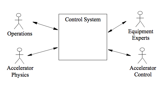
Figure 6: “Use Case” Approach.

As is often the case though, what today have become “Best Practices” for the design & implementation of software & hardware architectures for complex telecomm systems, originated from the solution of an intricate commercial Systems Engineering Problem in the 1980s. To quote I. Jacobson, 2010, one of the “Three Amigos” who with G. Booch and R. Rambaugh invented & developed the Unified Modeling Language (UML) for Software Engineering in the 1990s [68, 69, 70]:

It was like that in the late 1960s and the ‘70s when the Ericsson AXE system beat all competition and won every contract thanks to being component-based. Similarly, when Rational was successful because of UML and Objectory. And Telelogic because of SDL.

…

In 1986, Use Case was the solution to the problem that traditional functional specifications were immense and not testable. To start from the users and find their different use cases made the specifications understandable, while we also at the same time found the test cases. The result was a good way to do test-driven development, now being popular in agile teams.

Also, as G. Booch wrote in the foreword to “Design Patterns: Elements of Reusable Object-Oriented Software”, 1994 [75]:

All well-structured object-oriented architectures are full of patterns. Indeed, one of the ways that I measure the quality of an object-oriented system is to judge whether or not its developers have paid careful attention to the common collaborations among its objects. Focusing on such mechanisms during a system’s development can yield an architecture that is smaller, simpler, and far more understandable than if these patterns are ignored.

The importance of patterns in crafting complex systems has been long recognized in other disciplines. In particular, Christopher Alexander ([76]) and his colleagues were perhaps the first to propose the idea of using a pattern language to architect buildings and cities. His ideas and the contributions of others have now taken root in the object-oriented software community. In short, the concept of the design pattern provides a key to helping developers leverage the expertise of other skilled architects.

…

which was written by the “Gang of Four”: E. Gamma, R. Helm, R. Johnson, and J. Vlissides. Alexander’s work also inspired the implementation of the first Wiki by Cunningham [77].

Not surprisingly, to start from the End-User is part of the strategy for systematic database design as well. To quote T. Halpin [80]:

Although a rigorous process model is best built on top of a data model, an overview of the processes can be useful as a precursor to the data modeling, especially if the application is large or only vaguely understood. It is often helpful to get a clear picture of the functions of the application first.

Similarly, the field of Particle Accelerators has started to catch on [1, 27, 26, 29, 31, 32].

In conclusion, effective, goal oriented guidelines for how to pursue a systematic End-User oriented approach for the functional specs for a software architecture of arbitrary complexity; for e.g. model-based control, end-to-end testing of controls application before commissioning of the system, etc.

3.1 Lattice: Independent Parameters

The linearised beam dynamics model is a straightforward exercise in Hamiltonian Dynamics and Linear Control Theory.

The Hamiltonian is Eq. (10) ($\bar{x}\equiv\left[x,p_{x},y,p_{y},c_{0}t,-p_{t}\right]$)

$$H_{2}\left(\bar{x};s\right)=\frac{p_{x}^{2}+p_{y}^{2}}{2\left(1+p_{t}\right)}+\frac{b_{2}\left(s\right)}{2}\left(x^{2}-y^{2}\right)+\frac{x^{2}}{2\rho^{2}\left(s\right)}-\frac{xp_{t}}{\rho\left(s\right)}$$ (59)

i.e., what is defined by the Lattice File. The Equations of Motion for the horizontal plane are (Hamiltons Equations)

$$\begin{cases}x^{\prime}=&\partial_{p_{x}}H=\frac{p_{x}}{1+p_{t}}\\ p^{\prime}_{x}=&-\partial_{x}H=-b_{2}\left(s\right)x-\frac{x}{\rho^{2}\left(s\right)}+\frac{p_{t}}{\rho\left(s\right)}\\ y^{\prime}=&\partial_{p_{y}}H=\frac{p_{y}}{1+p_{t}}\\ p^{\prime}_{y}=&-\partial_{y}H=b_{2}\left(s\right)y\end{cases}$$ (60)

By taking the derivative

$$x^{\prime\prime}=\frac{p^{\prime}_{x}}{1+p_{t}},\qquad y^{\prime\prime}=\frac{p^{\prime}_{y}}{1+p_{t}}$$ (61)

the system of first order Ordinary Differential Equations (ODEs) can be reduced to a system of second order ODEs (Hill’s Equation [18])

$$\begin{cases}x^{\prime\prime}+\frac{K_{x}\left(s\right)}{1+p_{t}}x&=\frac{\delta}{\rho\left(s\right)\left(1+p_{t}\right)}\\ y^{\prime\prime}-\frac{K_{y}\left(s\right)}{1+p_{t}}y&=0\end{cases}$$ (62)

where

$$K_{x}\left(s\right)=b_{2}\left(s\right)-\frac{1}{\rho^{2}\left(s\right)},\qquad K_{y}\left(s\right)=-b_{2}\left(s\right).$$ (63)

The Lattice Parameters, typically piece-wise constant, i.e., independent, are summarized in Tab. 1.

The total energy is given by Eq. (2):

$$E_{\mathrm{b}}=\sqrt{\left(m_{0}c_{0}^{2}\right)^{2}+\left(pc_{0}\right)^{2}}.$$ (64)

Parameter Name	Symbol	Units
Beam Energy	$E_{\mathrm{b}}$	$\left[\mathrm{GeV}\right]$
Element Length	$L\left(s\right)$	$\left[\mathrm{m}\right]$
Dipole Bend Radius	$\rho\left(s\right)=\frac{L}{\phi}$	$\left[\mathrm{m}\right]$
Quadrupole Gradient	$b_{2}\left(s\right)$	$\left[\mathrm{m}^{-2}\right]$

Table 1: Lattice Parameters (independent).

3.2 Linear Optics: Dependent Parameters

The solution for a piece-wise constant $K\left(s\right)$ is the Transport Matrix obtained in Appendix A.6

$$\bar{x}_{j\rightarrow k}=M_{j\rightarrow k}\bar{x}_{0}$$ (65)

where $M_{j\rightarrow k}$ is the Transport Matrix from $j\rightarrow k$.

The Linear Dispersion & Optics (Twiss Parameters [42, 81]) are propagated by Eqs. (13) & (29)

$$\bar{\eta}_{k} =M_{j\rightarrow k}\bar{\eta}_{j},$$

$$A_{k}\left(\overline{\Delta\mu}_{k}\right) =M_{j\rightarrow k}A_{j}\left(\overline{\Delta\mu}_{j}\right),$$

$$\alpha_{k,\left[x,y\right]} =-m_{11}m_{21}-m_{12}m_{22},$$

$$\beta_{k,\left[x,y\right]} =m_{11}^{2}+m_{12}^{2}$$ (66)

where

$$A_{k}\left(\overline{\Delta\mu}_{k}\right)\equiv\left[\begin{array}[]{ccc}A_{k}\left(\Delta\mu_{x,k}\right)&0&0\\ 0&A_{k}\left(\Delta\mu_{y,k}\right)&0\\ 0&0&1\end{array}\right]$$ (67)

with the block diagonal sub matrices

$$A_{k}\left(\Delta\mu_{\left[x,y\right],k}\right)\equiv\left[\begin{array}[]{cc}m_{11}&m_{12}\\ m_{21}&m_{22}\end{array}\right]=\left[\begin{array}[]{cc}\sqrt{\beta_{k,\left[x,y\right]}}\cos\left(\Delta\mu_{k,\left[x,y\right]}\right)&\sqrt{\beta_{k,\left[x,y\right]}}\sin\left(\Delta\mu_{k,\left[x,y\right]}\right)\\ -\frac{\sin\left(\Delta\mu_{k,\left[x,y\right]}\right)+\alpha_{k,\left[x,y\right]}\cos\left(\Delta\mu_{k,\left[x,y\right]}\right)}{\sqrt{\beta_{k,\left[x,y\right]}}}&\frac{\cos\left(\Delta\mu_{k,\left[x,y\right]}\right)-\alpha_{x,k}\sin\left(\Delta\mu_{k,\left[x,y\right]}\right)}{\sqrt{\beta_{k,\left[x,y\right]}}}\end{array}\right].$$ (68)

Similarly, for a Periodic System the Linear Dispersion & Optics Functions are given by Eqs. (40), (56), and (57)

$$\bar{\eta} =\left(I-M\right)^{-1}D,$$

$$M =A_{0}R\left(2\pi\bar{\nu}\right)A_{0}^{-1},$$

$$A_{k}\left(\overline{\Delta\mu}_{k}\right) =M_{j\rightarrow k}A_{j}\left(\overline{\Delta\mu}_{j}\right),$$

$$\alpha_{\left[x,y\right],k} =-m_{11}m_{21}-m_{12}m_{22},$$

$$\beta_{\left[x,y\right],k} =m_{11}^{2}+m_{12}^{2}$$ (69)

where

$$D=\left[m_{16},m_{26},0,0,0,0\right]^{\mathrm{T}},$$ (70)

the 2nd equation a Matrix Diagonalization with

$$R\left(2\pi\bar{\nu}\right)\equiv\left[\begin{array}[]{ccc}R\left(\Delta\mu_{x,k}\right)&0&0\\ 0&R\left(\Delta\mu_{y,k}\right)&0\\ 0&0&1\end{array}\right],\qquad R\left(\Delta\mu\right)\equiv\left[\begin{array}[]{cc}\cos\left(\Delta\mu\right)&\sin\left(\Delta\mu\right)\\ -\sin\left(\Delta\mu\right)&\cos\left(\Delta\mu\right)\end{array}\right],$$ (71)

and the 3rd equation transports the Linear Optics Functions from the beginning of the Lattice.

The Local Linear Optics design parameters, i.e., dependent parameters, along the structure are:

Parameter Name	Symbol	Units
Hor. Linear Dispersion	$\bar{\eta}\left(s\right)\equiv\left[\eta_{x}\left(s\right),\eta^{\prime}_{x}\left(s\right)\right]$	$\left[\mathrm{m}\right]$
Beta Function	$\bar{\beta}\left(s\right)\equiv\left[\beta_{x}\left(s\right),\beta_{y}\left(s\right)\right]$	$\left[\mathrm{m}\right]$
Beta Function Derivative	$\bar{\alpha}\left(s\right)\equiv-\frac{1}{2}\partial_{s}\bar{\beta}\left(s\right)=\left[\alpha_{x}\left(s\right),\alpha_{y}\left(s\right)\right]$	$\left[.\right]$
Normalized Phase Advance	$\bar{\nu}\left(s\right)\equiv\frac{\bar{\mu}\left(s\right)}{2\pi}=\left[\frac{\mu_{x}\left(s\right)}{2\pi},\frac{\mu_{y}\left(s\right)}{2\pi}\right]$	$\left[.\right]$

Table 2: Local Linear Optics Design Parameters (dependent).

And the Global Linear Optics for a Periodic Cell are:

Parameter Name	Symbol	Units
Cell Tune	$\bar{\nu}\equiv\left[\frac{\mu_{x}\left(L_{\mathrm{tot}}\right)}{2\pi},\frac{\mu_{y}\left(L_{\mathrm{tot}}\right)}{2\pi}\right]$	$\left[\mathrm{.}\right]$
Linear Chromaticity	$\bar{\xi}\equiv\left[\xi_{x},\xi_{y}\right]$	$\left[\mathrm{.}\right]$
Horizontal Emittance	$\varepsilon_{x}$	$\left[\mathrm{pm\cdot rad}\right]$
Linear Dispersion Action	$\mathscr{H}_{x}$	$\left[\mathrm{m}\right]$
Momentum Spread	$\sigma_{\delta}$	$\left[.\right]$
Linear Momentum Compaction	$\alpha_{\mathrm{c}}$	$\left[\mathrm{.}\right]$
Energy Loss per Turn	$U_{0}$	$\left[\mathrm{eV}\right]$
Damping Times	$\bar{\tau}\equiv\left[\tau_{x},\tau_{y},\tau_{z}\right]$	$\left[\mathrm{msec}\right]$
Damping Partition Numbers	$\bar{J}\equiv\left[J_{x},J_{y},J_{z}\right]$	$\left[.\right]$
Total Length	$L_{\mathrm{tot}}$	$\left[\mathrm{m}\right]$
Total Bend Angle	$\phi_{\mathrm{tot}}$	$\left[\text{\textdegree}\right]$
Total Absolute Bend Angle	$\sum\left|\phi\right|$	$\left[\text{\textdegree}\right]$

Table 3: Global Linear Optics Properties for a Periodic Cell (dependent).

3.3 Optimal Problems

3.3.1 Least-Square Fit

The Merit Function for a Least-Square fit has the general form

$$\mathrm{Min}\left\{\chi^{2}\right\}=\sum_{k}c_{k}\left(y_{k}-y_{k}^{*}\left(x_{k};\bar{a}\right)\right)^{2}$$ (72)

where $\bar{x}$ are the initial conditions, $\bar{y}^{*},\bar{y}$ the resulting propagated and desired values, respectively, (e.g. for Linear Dispersion & Optics, see Tab. 2-3) $\bar{a}$ the independent parameters e.g. Lattice, see Tab. 1, and $\bar{c}$ arbitrary weight factors (since e.g. the units for the dependent parameters might be different). It can be solved numerically by using e.g. Powell’s Method [82, 83], Levenberg–Marquardt [84, 85], or Downhill Simplex [86].

3.3.2 Use Case: Beamline Matching

To Match a Beamline:

1. The Linear Optics Functions at the Cell Entrance $\bar{x}$ are given.

2. The desired values for the Linear Optics Functions at the Cell Exit $\bar{y}$ are given.

3. Suitable numerical weight coefficients $c_{k}$ are given; essentially, to numerically balance terms with different units & magnitude and relative importance.

4. The select Lattice Parameters $\bar{a}$ are set to the Initial Values $\bar{a}_{0}$.

5. The Linear Optics Functions at the Exit $\bar{y}\left(\bar{x};\bar{a}\right)$ are computed, for the given $\bar{x},\bar{a}_{0}$

   $$\begin{cases}\bar{\eta}_{k}&=M_{j\rightarrow k}\bar{\eta}_{j}\\ A_{k}\left(\bar{\Delta\mu}_{k}\right)&=M_{j\rightarrow k}A_{j}\left(\bar{\Delta\mu}_{j}\right)\\ \alpha_{\left[x,y\right],k}&=-m_{11}m_{21}-m_{12}m_{22}\\ \beta_{\left[x,y\right],k}&=m_{11}^{2}+m_{12}^{2}\end{cases}$$ (73)

6. The (merit) $\chi^{2}$-function is evaluated; i.e., a measure for how much the computed values $\bar{y}^{*}\left(\bar{x};\bar{a}\right)$ deviate from the desired $\bar{y}$.

7. The Lattice Parameters $\bar{a}$ are varied to minimize $\chi^{2}$.

8. Repeat until within desired precision or maximum number of iterations.

A summary is given in Tab. 4. For an example (of a MATLAB implementation based on “Accelerator Toolbox”) see ref. [87].

Parameter Name	Initial Value $\bar{a}_{0}$	Final Value $\bar{a}_{1}$	Initial Value $\bar{x}$	Final Value $\bar{y}^{*}$	Desired Value $\bar{y}$	Delta
Element Length	$\bar{L}_{0}$	$\bar{L}_{1}$
Bend Radius	$\bar{\rho}_{0}$	$\bar{\rho}_{1}$
Gradient	$\bar{b}_{2,0}$	$\bar{b}_{2,1}$
Dispersion			$\bar{\eta}_{0}$	$\bar{\eta}_{1}^{*}$	$\bar{\eta}_{1}$	$\bar{\eta}_{1}^{*}-\bar{\eta}_{1}$
Dispersion Derivative			$\bar{\eta}^{\prime}_{0}$	$\bar{\eta}{}_{1}^{{}^{\prime}*}$	$\bar{\eta}^{\prime}_{1}$	$\bar{\eta}{}_{1}^{{}^{\prime}*}-\bar{\eta}^{\prime}_{1}$
Beta Function			$\bar{\beta}_{0}$	$\bar{\beta}_{1}^{*}$	$\bar{\beta}_{1}$	$\bar{\beta}_{1}^{*}-\bar{\beta}_{1}$
Beta Function Derivative			$\bar{\alpha}_{0}$	$\bar{\alpha}_{1}^{*}$	$\bar{\alpha}_{1}$	$\bar{\alpha}_{1}^{*}-\bar{\alpha}_{1}$

Table 4: Matching: Independent and Dependent Parameters.

Figure 7: Matching.

3.3.3 Use Case: Periodic Cell

To optimize a Periodic Solution is akin to Beamline Matching, but the computation is done for the periodic solution with periodic constraints.

1. Suitable numerical weight coefficients $c_{k}$ are given; essentially, to numerically balance terms with different units & magnitude and relative importance.

2. The select Lattice Parameters $\bar{a}$ are set to the Initial Values $\bar{a}_{0}$.

3. The Periodic Linear Optics Functions $\bar{y}\left(\bar{x};\bar{a}\right)$ are computed, for the given $\bar{x},\bar{a}_{0}$

   $$\begin{cases}\bar{\eta}&=\left(I-M\right)^{-1}D\\ M&=A_{0}R\left(2\pi\bar{\nu}\right)A_{0}^{-1}\\ A_{k}\left(\bar{\Delta\mu}_{k}\right)&=M_{j\rightarrow k}A_{j}\left(\bar{\Delta\mu}_{j}\right)\\ \beta_{k,\left[x,y\right]}&=m_{11}^{2}+m_{12}^{2}\\ \varepsilon_{x}&=C_{\mathrm{q}}\gamma^{2}\frac{I_{5}}{I_{2}-I_{4}}\end{cases}$$ (74)

   where the synchtrotron integrals $I_{2},I_{4},I_{5}$ are given by Eqs. (162).

4. The (merit) $\chi^{2}$-function is evaluated; i.e., a measure for how much the computed values $\bar{y}^{*}\left(\bar{x};\bar{a}\right)$ deviate from the desired $\bar{y}$.

5. The Lattice Parameters $\bar{a}$ are varied to minimize $\chi^{2}$.

A summary is given in Tab. 5. For an example (of a MATLAB implementation based on “Accelerator Toolbox”) see ref. [87].

Parameter Name	Initial Value $\bar{a}_{0}$	Final Value $\bar{a}_{1}$	Computed Value $\bar{y}^{*}$	Desired Value $\bar{y}$	Delta
Element Length	$\bar{L}_{0}$	$\bar{L}_{1}$
Bend Radius	$\bar{\rho}_{0}$	$\bar{\rho}_{1}$
Gradient	$\bar{b}_{2,0}$	$\bar{b}_{2,1}$
Dispersion			$\bar{\eta}^{*}$	$\bar{\eta}$	$\bar{\eta}^{*}-\bar{\eta}$
Dispersion Derivative			$\bar{\eta}^{\prime*}$	$\bar{\eta}^{\prime}$	$\bar{\eta}^{\prime*}-\bar{\eta}^{\prime}$
Beta Function			$\bar{\beta}^{*}$	$\bar{\beta}$	$\bar{\beta}^{*}-\bar{\beta}$
Cell Tune			$\bar{\nu}^{*}$	$\bar{\nu}$	$\bar{\nu}^{*}-\bar{\nu}$
Hor. Emittance			$\varepsilon_{x}^{*}$	$\varepsilon_{x}$	$\varepsilon_{x}^{*}-\varepsilon$

Table 5: Periodic Cell: Independent and Dependent Parameters.

Figure 8: Periodic Cell.

3.3.4 Use Case: Lattice Design

Generally speaking, synchrotron lattices are constructed from repetitive blocks comprising of unit cells & matching sections/dispersion suppressors for straight sections. The unit cell can be e.g. a FODO cell for beam transport for colliders or a low emittance cell for synchrotron light sources. Whereas the matching cells provide for interaction regions or space for insertion devices.

Hence, from the two outlined Use Cases¸ sections 3.3.2 & 3.3.3, two "building blocks" are obtained from which a prototype ring structure with an arbitrary number of unit cells & straight sections – with adjacent matching cells – can be constructed. After which more detailed design of the local linear optics can be pursued.

4 Conclusions

For a systematic, first principles approach, the formula relevant for Linear Optics design of Synchrotrons have been derived by Hamiltonian Dynamics. Equipped with these, the relevant “Use Cases” have then been captured providing a streamlined approach. In particular, to enable professionals, i.e., Software Engineers, to efficiently prototype & architect a CAD Tool for ditto.

We conjecture that the resulting Tools & Approach will generate a Paradigm Shift for Robust Linear Optics Design; i.e., better designs will be found by enabling the Linear Optics Designer to systematically & effectively explore the Full Parameter Space for a Prototype Lattice Design interactively. Besides, the approach might lead to a closer & more streamlined approach & collaboration with Engineers; since a state-of-the-art design is a matter of Engineering-Science; e.g. MAX-IV [46, 47, 48].

Appendices

Appendix A Relativistic Hamiltonian

A.1 Hamiltonian

The relativistic Hamiltonian for a charged particle with charge $q$ and energy $E$ in an external electromagnetic field with vector potential $\bar{A}$ – for the co-moving system, customarily used to model particle accelerators – is ($\bar{x}=\left[x,p_{x},y,p_{y},t,-\varepsilon\right]$) [19, 57]

$$H\left(\bar{x};s\right)=-p_{s}=-\left(1+h\left(s\right)x\right)\left[\frac{q}{p_{0}}A_{s}+\sqrt{\left(\frac{\varepsilon}{c_{0}}-\frac{q\Phi\left(s\right)}{p_{0}c_{0}}\right)^{2}-\frac{1}{\beta_{0}^{2}\gamma_{0}^{2}}-\left(p_{x}-\frac{qA_{x}\left(s\right)}{p_{0}}\right)^{2}-\left(p_{y}-\frac{qA_{y}\left(s\right)}{p_{0}}\right)^{2}}\right]$$ (75)

where $\left[\beta,\gamma\right]$ are the relativistic factors

$$\gamma\equiv\frac{1}{\sqrt{1-\beta^{2}}}=\frac{E}{m_{0}c_{0}^{2}},\qquad\varepsilon\equiv\frac{E}{p_{0}}$$ (76)

and

$$h\left(s\right)\equiv\frac{1}{\rho\left(s\right)}$$ (77)

is the local curvature for the reference trajectory, see Fig. (2).

Introducing longitudinal coordinates relative to the reference particle and scaling with $c_{0}$

$$c_{0}T\equiv\left(t-\frac{s}{v_{0}}\right)c_{0},\qquad P_{t}\equiv\frac{E-E_{0}}{p_{0}c_{0}}=\frac{\Delta E}{p_{0}c_{0}}=\frac{\varepsilon-\varepsilon_{0}}{c_{0}}=\frac{\varepsilon}{c_{0}}-\frac{1}{\beta_{0}}$$ (78)

by the canonical transformation

$$F_{2}\left(t,P_{t}\right)=\left(t-\frac{s}{v_{0}}\right)c_{0}\left(\frac{1}{\beta_{0}}+P_{t}\right)$$ (79)

gives

$$\begin{cases}c_{0}T&=\partial_{P_{t}}F_{2}=\left(t-\frac{s}{v_{0}}\right)c_{0}\\ -\varepsilon&=\partial_{t}F_{2}=c_{0}\left(\frac{1}{\beta_{0}}+P_{t}\right)\\ K&=\partial_{s}F_{2}=\frac{1}{\beta_{0}^{2}}+\frac{P_{t}}{\beta_{0}}\end{cases}$$ (80)

and the new Hamiltonian is ($\bar{x}=\left[x,p_{x},y,p_{y},c_{0}t,-p_{t}\right]$)

$$H\left(\bar{x};s\right)=\frac{p_{t}}{\beta_{0}}-\left(1+h\left(s\right)x\right)\left[\frac{q}{p_{0}}A_{s}+\sqrt{\left(\frac{1}{\beta_{0}}+p_{t}-\frac{q\Phi\left(s\right)}{p_{0}c_{0}}\right)^{2}-\frac{1}{\beta_{0}^{2}\gamma_{0}^{2}}-\left(p_{x}-\frac{qA_{x}\left(s\right)}{p_{0}}\right)^{2}-\left(p_{y}-\frac{qA_{y}\left(s\right)}{p_{0}}\right)^{2}}\right]$$ (81)

ignoring the constant term $\nicefrac{{1}}{{\beta_{0}^{2}}},$using $H$ for the new Hamiltonian, and small letters for the new phase-space coordinates.

The equations of motions are (Hamilton’s equations, $\bar{x}\equiv\left[q^{1},p_{1},q^{2},p_{2},\ldots\right]$)

$$\bar{x}^{\prime}=\left\{-H,\bar{x}\right\}=-\left(\left(\nabla_{\bar{x}}H\right)\Omega\right)^{\mathrm{T}}=\left[\partial_{p_{1}}H,-\partial_{q^{1}}H,\partial_{p_{2}}H,-\partial_{q^{2}}H,\ldots\right]^{\mathrm{T}}$$ (82)

where (Poisson Bracket)

$$\left\{-H,\cdot\right\}\equiv-\sum_{k}\left[\left(\partial_{q^{k}}H\right)\partial_{p_{k}}-\left(\partial_{p_{k}}H\right)\partial_{q^{k}}\right]$$ (83)

and (symplectic form, from Greek intertwined)

$$\Omega\equiv\left[\begin{array}[]{ccc}\Omega_{x}&0&0\\ 0&\Omega_{y}&0\\ 0&0&\Omega_{s}\end{array}\right],\qquad\Omega_{x,y,s}=\left[\begin{array}[]{cc}0&1\\ -1&0\end{array}\right].$$ (84)

N.B. The upper & lower indeces are a reflection of the corresponding differential forms/geometry; i.e., a point of the cotangent bundle $T^{\ast}V$ (i.e., phase-space) is specified by the coordinates $\left[q^{i},p_{j}\right]$.

The fundamental Poissan brackets are (Lie algebra)

$$\left\{q^{i},p_{j}\right\}=\delta_{j}^{i},\qquad\left\{q^{i},q^{j}\right\}=\left\{p_{i},p_{j}\right\}=0$$ (85)

and the Hamiltonian flow’s divergence is (vs. a general vector flow)

$$\nabla_{\bar{x}}\cdot\bar{x}^{\prime}=\nabla_{\bar{x}}\cdot\left\{-H,\bar{x}\right\}=0$$ (86)

i.e., the symplectic flow in phase-space is akin to an incompressible fluid; for a time independent Hamiltonian.

Rather than integrating, etc., it is more expedient and transparent to utilize the Lie Series solution [59, 60] for the Poincaré map (introduced to celestial mechanics 1960)

$$\bar{x}_{1}=\mathscr{M}\bar{x}_{0}=e^{\mathscr{D}\left(-H\right)}\bar{x}_{0}\equiv\sum_{k=0}^{\infty}\frac{\mathscr{D}^{k}\left(-H\right)}{k!}\bar{x}_{0}$$ (87)

where (Lie derivative)

$$\mathscr{D}\left(-H\right)=\left\{-H,\cdot\right\}.$$ (88)

A.2 Multipole Expansion

The magnetic multipole expansion is introduced by (polar coordinates for $\left[x,y\right]$)

$$B_{y}\left(s\right)+iB_{x}\left(s\right) \equiv\left(B\rho\right)\sum_{n=1}^{\infty}\left(ia_{n}\left(s\right)+b_{n}\left(s\right)\right)\left(re^{i\varphi}\right)^{n-1}$$

$$=\left(B\rho\right)\sum_{n=1}^{\infty}\left(ia_{n}\left(s\right)+b_{n}\left(s\right)\right)\left(x+iy\right)^{n-1}$$ (89)

where (magnetic rigidity)

$$\left(B\rho\right)\equiv\frac{p}{q}$$ (90)

see Fig. (3).

The corresponding vector potential is obtained from (Poincaré gauge, $\bar{r}\cdot\bar{A}=0$) [58]

$$\bar{A}\left(\bar{r},t\right)=-\bar{r}\times\intop_{0}^{1}\bar{B}\left(u\bar{r},t\right)udu,\qquad\phi=-\bar{r}\cdot\intop_{0}^{1}\bar{B}\left(u\bar{r},t\right)udu$$ (91)

which gives (Cartesian coordinates for $\left[x,s\right]$, $h\left(s\right)=0$ )

$$\begin{cases}A_{x}=A_{y}&=0\\ \frac{q}{p_{0}}A_{s}\left(s\right)&=\mathrm{Re}\sum_{n=1}^{\infty}\frac{1}{n}\left(ia_{n}\left(s\right)+b_{n}\left(s\right)\right)\left(re^{i\varphi}\right)^{n}\\ &=\mathrm{Re}\sum_{n=1}^{\infty}\frac{1}{n}\left(ia_{n}\left(s\right)+b_{n}\left(s\right)\right)\left(x+iy\right)^{n}.\end{cases}$$ (92)

For a sector bend (polar coordinates for $\left[x,s\right]$, arc reference trajectory)

$$\frac{q}{p_{0}}A_{s}=-b_{0}\left(x-\frac{hx^{2}}{2\left(1+hx\right)}\right)=-\frac{b_{0}x\left(2+hx\right)}{2\left(1+hx\right)},\qquad h=b_{0}.$$ (93)

For completeness, correspondingly, the field, curl$\bar{B}\equiv\bar{\nabla}\times\bar{A}$, in the curvilinear co-moving frame is [19]

$$B_{x}=\frac{\partial_{z}A_{y}-\partial_{y}A_{z}}{1+h\left(s\right)x},\qquad B_{y}=\frac{h\left(s\right)A_{s}}{1+h\left(s\right)x}+\partial_{x}A_{s}-\frac{\partial_{s}A_{x}}{1+h\left(s\right)x},\qquad B_{z}=\partial_{y}A_{x}-\partial_{x}A_{y}.$$ (94)

A.3 Paraxial Approximation

For the paraxial approximation $p_{x,y}\ll 1$ the Hamiltonian simplifies to (not expanded in $p_{t}$ by first factoring out $1+\delta\left(p_{t}\right)$)

$$H\left(\bar{x};s\right)=\frac{\left(p_{x}-\frac{qA_{x}\left(s\right)}{p_{0}}\right)^{2}+\left(p_{y}-\frac{qA_{y}\left(s\right)}{p_{0}}\right)^{2}}{2\left(1+\delta\left(p_{t}\right)\right)}-\left(1+h\left(s\right)x\right)\left(\frac{qA_{s}\left(s\right)}{p_{0}}+1+\delta\left(p_{t}\right)\right)+\frac{q\Phi\left(s\right)}{p_{0}c_{0}}+\ldots$$ (95)

where

$$1+\delta\left(p_{t}\right)=\frac{p\left(p_{t}\right)}{p_{0}}=\sqrt{1+\frac{2p_{t}}{\beta_{0}}+p_{t}^{2}}=\frac{\beta\gamma}{\beta_{0}\gamma_{0}},\qquad\delta\left(p_{t}\right)\equiv\frac{p\left(p_{t}\right)-p_{0}}{p_{0}}$$ (96)

By inserting to multipole expansion Eq. (92), to leading order one obtains (quadratic Hamiltonian)

$$H_{2}\left(\bar{x};s\right)=\frac{p_{x}^{2}+p_{y}^{2}}{2\left(1+\delta\left(p_{t}\right)\right)}+\frac{K_{x}\left(s\right)x^{2}}{2}-\frac{K_{y}\left(s\right)y^{2}}{2}-\frac{h\left(s\right)xp_{t}}{\beta_{0}}+\frac{p_{t}^{2}}{2\beta_{0}^{2}\gamma_{0}^{2}}+\frac{q\Phi\left(s\right)}{p_{0}c_{0}}$$ (97)

where

$$K_{x}\left(s\right)\equiv b_{2}\left(s\right)+h^{2}\left(s\right),\qquad K_{y}\left(s\right)\equiv b_{2}\left(s\right).$$ (98)

A.4 Dispersion

The inhomogeneous term $\nicefrac{{h\left(s\right)xp_{t}}}{{\beta_{0}}}$ is removed from the quadratic Hamiltonian Eq. (97) by introducing the dispersion function

$$\bar{x}\left(s,\delta\right)\equiv\eta{}_{x}\left(s\right)\delta\left(p_{t}\right)$$ (99)

which by inserting into Hamilton’s equations

$$\left\{\begin{aligned} x^{\prime}&=\partial_{p_{x}}H_{2}=\frac{p_{x}}{1+\delta\left(p_{t}\right)}\\ p_{x}^{\prime}&=-\partial_{x}H_{2}=-K_{x}\left(s\right)x+h\left(s\right)\delta\left(p_{t}\right)\end{aligned}\right.$$ (100)

gives

$$\eta^{\prime\prime}{}_{x}+\frac{K_{x}\left(s\right)}{1+\delta\left(p_{t}\right)}\eta{}_{x}=\frac{h\left(s\right)}{1+\delta\left(p_{t}\right)}$$ (101)

and the periodic solution can be obtained by solving perturbatively

$$\eta_{x}\left(s\right)=\eta_{x}^{\left(1\right)}\left(s\right)+\eta_{x}^{\left(2\right)}\left(s\right)\delta\left(p_{t}\right)+\ldots$$ (102)

The Poincaré map is ($\bar{x}_{k}\equiv\left[x,p_{x}\right]$)

$$\bar{x}_{k+1}=M\bar{x}_{k}+Dp_{t}$$ (103)

where

$$M=\left[\begin{array}[]{cc}\cos\left(2\pi\nu_{x}\right)+\alpha_{x}\sin\left(2\pi\nu_{x}\right)&\beta_{x}\sin\left(2\pi\nu_{x}\right)\\ -\gamma_{x}\sin\left(2\pi\nu_{x}\right)&\cos\left(2\pi\nu_{x}\right)-\alpha_{x}\sin\left(2\pi\nu_{x}\right)\end{array}\right],\qquad D=\left[\begin{array}[]{c}m_{16}\\ m_{26}\end{array}\right]$$ (104)

and the periodic solution is given by

$$\bar{\eta}=M\bar{\eta}+D\Rightarrow\bar{\eta}=\left(I-M\right)^{-1}D$$ (105)

which gives

$$\bar{\eta}=\left[\begin{array}[]{cc}\frac{1+\alpha_{x}\cot\left(\pi\nu_{x}\right)}{2}&\frac{\beta_{x}\cot\left(\pi\nu_{x}\right)}{2}\\ -\frac{\gamma_{x}\cot\left(\pi\nu_{x}\right)}{2}&\frac{1-\alpha_{x}\cot\left(\pi\nu_{x}\right)}{2}\end{array}\right]\left[\begin{array}[]{c}m_{16}\\ m_{26}\end{array}\right].$$ (106)

The new Hamiltonian is obtained by the generating function [19]

$$F_{2}\left(x,t,P_{x},P_{t};s\right)=\left(x-\eta_{x}\left(s\right)\delta\left(P_{t}\right)\right)\left(P_{x}+\eta^{\prime}_{x}\left(s\right)\delta\left(P_{t}\right)\left(1+\delta\left(P_{t}\right)\right)\right)+\frac{1}{2}\eta_{x}\left(s\right)\eta^{\prime}_{x}\left(s\right)\delta^{2}\left(P_{t}\right)\left(1+\delta\left(P_{t}\right)\right)+c_{0}tP_{t}$$ (107)

which gives

$$\left\{\begin{aligned} X&=\partial_{P_{x}}F_{2}=x-\eta{}_{x}\left(s\right)\delta\left(P_{t}\right)\\ p_{x}&=\partial_{x}F_{2}=P_{x}+\eta^{\prime}_{x}\left(s\right)\delta\left(P_{t}\right)\left(1+\delta\left(P_{t}\right)\right)\\ c_{0}T&=\partial_{P_{t}}F_{2}=c_{0}t-\frac{\frac{1}{\beta_{0}}+p_{t}}{\sqrt{1+\frac{2p_{t}}{\beta_{0}}+p_{t}^{2}}}[\eta_{x}\left(s\right)P_{x}-\eta^{\prime}_{x}\left(s\right)\left(X+2X\delta\left(P_{t}\right)+\frac{1}{2}\eta_{x}\left(s\right)\delta^{2}\left(P_{t}\right)\right)]\\ p_{t}&=\partial_{c_{0}t}F_{2}=\delta\left(P_{t}\right)\\ K_{2}\left(X,P_{x};s\right)&=H_{2}\left(\bar{x};s\right)+\partial_{s}F_{2}\left(x,P_{x};s\right)\end{aligned}\right.$$ (108)

and

$$H_{2}\left(\bar{x};s\right)=\frac{p_{x}^{2}+p_{y}^{2}}{2\left(1+p_{t}\right)}+\frac{K_{x}\left(s\right)x^{2}}{2}-\frac{K_{y}\left(s\right)y^{2}}{2}-\frac{\left(h\left(s\right)\eta_{x}\left(s\right)-\frac{1}{\beta_{0}^{2}\gamma_{0}^{2}}\right)p_{t}^{2}}{2}+\frac{q\Phi\left(s\right)}{p_{0}c_{0}}$$ (109)

using $H$ for the new Hamiltonian and small letters for the new phase-space coordinates.

N.B.: In the longitudinal plane, dispersion generates amplitude dependence of the path length – due to coupling between the planes – which can e.g. drive synchro-betatron resonances.

A.5 Momentum Compaction

Averaging over one turn in the longitudinal plane – since the synchtrotron frequency is much lower than the betatron, $\nu_{s}\ll\nu_{x,y}$ – gives (adiabatic approximation) [88]

$$\left\langle H_{2}\left(\bar{x};s\right)\right\rangle_{s}= \frac{p_{x}^{2}+p_{y}^{2}}{2\left(1+\delta\left(p_{t}\right)\right)}+\frac{K_{x}\left(s\right)x^{2}}{2}-\frac{K_{y}\left(s\right)y^{2}}{2}-\frac{\left(\left\langle\frac{h\left(s\right)\eta_{x}\left(s\right)}{2}\right\rangle_{s}-\frac{1}{\beta_{0}^{2}\gamma_{0}^{2}}\right)p_{t}^{2}}{2}+\frac{q\Phi\left(s\right)}{p_{0}c_{0}}+\ldots$$

$$= \frac{p_{x}^{2}+p_{y}^{2}}{2\left(1+\delta\left(p_{t}\right)\right)}+\frac{K_{x}\left(s\right)x^{2}}{2}-\frac{K_{y}\left(s\right)y^{2}}{2}-\frac{\eta_{\mathrm{c}}\left(p_{t}\right)p_{t}^{2}}{2}+\frac{q\Phi\left(s\right)}{p_{0}c_{0}}+\ldots$$ (110)

where $\eta_{\mathrm{c}}\left(p_{t}\right)$ (closed orbit phase slip factor)

$$\eta_{\mathrm{c}}\left(p_{t}\right)\equiv\frac{\nicefrac{{\left(T-T_{0}\right)}}{{T_{0}}}}{\nicefrac{{\left(E-E_{0}\right)}}{{E_{0}}}}=\frac{\nicefrac{{\left(C-C_{0}\right)}}{{T_{0}}}}{\nicefrac{{\left(E-E_{0}\right)}}{{E_{0}}}}-\frac{\beta-\beta_{0}}{\beta_{0}}=\alpha_{\mathrm{c}}\left(p_{t}\right)-\frac{1}{\beta_{0}^{2}\gamma_{0}^{2}}$$ (111)

and (momentum compaction)

$$\alpha_{\mathrm{c}}\left(p_{t}\right)\equiv\frac{\nicefrac{{\left(C-C_{0}\right)}}{{C_{0}}}}{\nicefrac{{\left(E-E_{0}\right)}}{{E_{0}}}}=\frac{1}{C}\ointop\frac{\eta_{x}\left(s\right)}{\rho\left(s\right)}ds=\alpha_{\mathrm{c}}^{\left(1\right)}+\alpha_{\mathrm{c}}^{\left(2\right)}\frac{E-E_{0}}{E_{0}}+\ldots$$ (112)

The equations of motion for the time-of-flight to leading order for $p_{x}=p_{y}=0$ is

$$c_{0}t^{\prime}=\frac{c_{0}}{\dot{s}}=\partial_{-p_{t}}H_{2}=\eta_{\mathrm{c}}p_{t}=\eta_{\mathrm{c}}\frac{\Delta E}{p_{0}c_{0}}=\eta_{\mathrm{c}}\frac{\Delta E}{\beta_{0}E_{0}}$$ (113)

which gives

$$\beta_{0}c_{0}t^{\prime}=\eta_{\mathrm{c}}\frac{\Delta E}{E_{0}}.$$ (114)

A.6 Betatron Motion: Action-Angle Coordinates

The Hamiltonian for the horizontal plane is Eq. (10)

$$H_{2}\left(\bar{x};s\right)=\frac{p_{x}^{2}}{2\left(1+p_{t}\right)}+\frac{K\left(s\right)x^{2}}{2}$$ (115)

and the equations of motion are (Hamilton’s equations)

$$\left\{\begin{aligned} x^{\prime}&=\partial_{p_{x}}H_{2}=\frac{p_{x}}{1+p_{t}}\\ p^{\prime}_{x}&=-\partial_{x}H_{2}=-K\left(s\right)x\end{aligned}\right.$$ (116)

which can be combined into (Hill’s equation)

$$x^{\prime\prime}+\frac{K\left(s\right)}{1+p_{t}}x=0.$$ (117)

The pseudo-harmonic oscillator ansatz ()

$$x\left(s;\delta\right)=\sqrt{\beta_{x}\left(s;\delta\right)}e^{\pm i\psi_{x}\left(s;\delta\right)},\qquad\alpha_{x}\left(s;\delta\right)\equiv-\frac{1}{2}\partial_{s}\beta_{x}\left(s;\delta\right)$$ (118)

gives

$$\left(\sqrt{\beta_{x}}\right)^{\prime\prime}+K\left(s\right)\sqrt{\beta_{x}}-\sqrt{\beta_{x}}\left(\psi^{\prime}_{x}\right)^{2}\pm i\left(\sqrt{\beta_{x}}\psi^{\prime\prime}_{x}+\frac{\beta^{\prime}_{x}}{\sqrt{\beta_{x}}}\psi^{\prime}_{x}\right)=0$$ (119)

which yields the relations

$$\left\{\begin{aligned} \left(\sqrt{\beta_{x}}\right)^{\prime\prime}+K\left(s\right)\sqrt{\beta_{x}}-\sqrt{\beta_{x}}\left(\psi^{\prime}_{x}\right)^{2}&=0\\ \frac{\psi^{\prime\prime}_{x}}{\psi^{\prime}_{x}}&=-\frac{\beta^{\prime}_{x}}{\beta_{x}}\end{aligned}\right.$$ (120)

and integrating the second equation gives

$$\psi{}_{x}\left(s;\delta\right)=\mu_{x}\left(s;\delta\right)+\phi_{x},\qquad\mu_{x}\left(s;\delta\right)\equiv\int_{0}^{s}\frac{du}{\beta_{x}\left(u;\delta\right)}$$ (121)

where $\mu_{x}\left(s\right)$ is the Courant & Snyder phase-advance. The global parameters $\left[\alpha,\beta,\mu\right]$ are called the Twiss parameters for the lattice [42, 81].

Action-angle coordinates $\left[J_{x},\psi_{x}\right]$ are introduced by the generating function [90]

$$F_{1}\left(x,\psi_{x};s\right)=-\frac{x^{2}}{2\beta_{x}\left(s;p_{t}\right)}\left(\tan\left(\psi_{x}\right)+\alpha_{x}\left(s;p_{t}\right)\right)$$ (122)

with

$$\left\{\begin{aligned} p_{x}&=-\partial_{x}F_{1}=-\frac{x}{\beta_{x}}\left(\tan\left(\psi_{x}\right)+\alpha_{x}\right)\\ J_{x}&=-\partial_{\psi_{x}}F_{1}=\frac{x^{2}}{2\beta_{x}\cos^{2}\left(\psi_{x}\right)}\\ K_{2}&=H_{2}+\partial_{s}F_{1}\end{aligned}\right.$$ (123)

Inverting the first and second equation gives

$$\left\{\begin{aligned} \psi_{x}\left(x,p_{x}\right)&=\mu_{x}\left(s;\delta\right)-\operatorname{atan2}2\left(\frac{\tilde{p}_{x}}{\tilde{x}}\right)=-\operatorname{atan2}2\left(\frac{\alpha_{x}\left(s;\delta\right)x+\beta_{x}\left(s;\delta\right)p_{x}}{x}\right)\\ 2J_{x}\left(x,p_{x}\right)&=\left|\tilde{x}\right|^{2}=\tilde{x}^{2}+\tilde{p}_{x}^{2}=\bar{x}^{\mathrm{T}}\left(AA^{\mathrm{T}}\right)^{-1}\left(s\right)\bar{x}=\gamma_{x}\left(s;\delta\right)x^{2}+2\alpha_{x}\left(s;\delta\right)xp_{x}+\beta_{x}\left(s;\delta\right)p_{x}^{2}\end{aligned}\right.$$ (124)

where (Floquet space)

$$\tilde{x}=A^{-1}\bar{x}$$ (125)

with

$$A=\left[\begin{array}[]{cc}\sqrt{\beta_{x}}&0\\ -\frac{\alpha_{x}}{\sqrt{\beta_{x}}}&\frac{1}{\sqrt{\beta_{x}}}\end{array}\right],\qquad A^{-1}=\left[\begin{array}[]{cc}\frac{1}{\sqrt{\beta_{x}}}&0\\ \frac{\alpha_{x}}{\sqrt{\beta_{x}}}&\sqrt{\beta_{x}}\end{array}\right]$$ (126)

see Fig. (4).

Conversely

$$\left\{\begin{aligned} x\left(s\right)&=\sqrt{2J_{x}\beta_{x}\left(s;\delta\right)}\cos\left(\psi_{x}\left(s;p_{t}\right)\right)\\ p_{x}\left(s\right)&=-\sqrt{\frac{2J_{x}}{\beta_{x}\left(s;\delta\right)}}\left(\sin\left(\psi_{x}\left(s;p_{t}\right)\right)+\alpha_{x}\left(s;p_{t}\right)\cos\left(\psi_{x}\left(s;p_{t}\right)\right)\right)\\ &=-\sqrt{2J_{x}\gamma_{x}\left(s;\delta\right)}\sin\left(\psi_{x}\left(s;p_{t}\right)+\arctan\left(\alpha_{x}\left(s;p_{t}\right)\right)\right)\end{aligned}\right.$$ (127)

see Fig. (5).

The action in diagonal form is

$$2J_{x}=\tilde{x}^{\mathrm{T}}\tilde{x}=\lambda_{+}\tilde{x}^{2}+\lambda_{-}\tilde{p}_{x}^{2}=\frac{\tilde{x}^{2}}{a^{2}}+\frac{\tilde{p}_{x}^{2}}{b^{2}},\qquad\lambda_{\pm}=h\pm\sqrt{h^{2}-1},\qquad h=\frac{\beta_{x}+\gamma_{x}}{2}$$ (128)

i.e., the ellipse parameters for the quadratic form are

$$a,b =\sqrt{\lambda_{\pm}}=\sqrt{h\pm\sqrt{h^{2}-1}}=\frac{1}{\sqrt{2}}\left(\sqrt{h+1}\pm\sqrt{h-1}\right),$$

$$\tan\left(2\xi_{x}\right) =\frac{2a_{12}}{a_{11}-a_{22}}=\frac{2\alpha_{x}}{\gamma_{x}-\beta_{x}},$$

$$\mathrm{Area} =\frac{\pi ab}{4}=\frac{\pi}{4}$$ (129)

where $\psi_{x}$ is the major’s angle relative to the $x$-axis; a phase-space rotation which diagonalizes $AA^{\mathrm{T}}$. Note, $\xi_{x}$ is not the phase advance $\psi_{x}$; which is determined by the particular choice of $A$, Eq. (22).

The equation for the ellipse with the transformed coordinates is

$$\left\{\begin{aligned} \tilde{x}\left(s\right)&=a\cos\left(\tilde{\psi}_{x}\right)\\ \tilde{p}_{x}\left(s\right)&=-b\sin\left(\tilde{\psi_{x}}\right)\end{aligned}\right..$$ (130)

The Poincaré map is

$$\bar{x}_{k+1}=M\bar{x}_{k}$$ (131)

where

$$M=\left[\begin{array}[]{cc}\cos\left(\mu_{x}\right)+\alpha_{x}\sin\left(\mu_{x}\right)&\beta_{x}\sin\left(\mu_{x}\right)\\ -\gamma_{x}\sin\left(\mu_{x}\right)&\cos\left(\mu_{x}\right)-\alpha_{x}\sin\left(\mu_{x}\right)\end{array}\right]$$ (132)

since (diagonal form)

$$M=AR\left(\mu_{x}\right)A^{-1},\qquad R\left(\mu_{x}\right)\equiv\left[\begin{array}[]{cc}\cos\left(\mu_{x}\right)&\sin\left(\mu_{x}\right)\\ -\sin\left(\mu_{x}\right)&\cos\left(\mu_{x}\right)\end{array}\right].$$ (133)

The new Hamiltonian is

$$K_{2}\left(J_{x},\psi_{x};s\right)=H_{2}+\frac{\alpha_{x}xp_{x}}{\beta_{x}}-\frac{\alpha^{\prime}_{x}x^{2}}{2\beta_{x}}=\frac{J_{x}}{\beta_{x}\left(s;p_{t}\right)}$$ (134)

where Eq. (117) has been used to simplify the expression.

The equations of motion are (Hamilton’s equations)

$$\left\{\begin{aligned} J^{\prime}_{x}&=-\partial_{\phi_{x}}K_{2}=0\\ \psi^{\prime}_{x}&=\partial_{J_{x}}K_{2}=\frac{1}{\beta_{x}\left(s;p_{t}\right)}\end{aligned}\right.$$ (135)

and by integrating

$$\left\{\begin{aligned} J_{x}&=\mathrm{cst}.\\ \psi{}_{x}&=\int_{0}^{s}\frac{du}{\beta_{x}\left(u;p_{t}\right)}+\phi_{x}=\mu_{x}\left(s;\delta\right)+\phi_{x}\end{aligned}\right.$$ (136)

where $\left[\phi_{x},J_{x}\right]$ are the constants of motion.

Averaging the Hamiltonian over one turn

$$\left\langle K_{2}\left(J_{x},\psi_{x};s\right)\right\rangle=\frac{J_{x}}{C}\int_{0}^{C}\frac{ds}{\beta_{x}\left(s;p_{t}\right)}=\frac{J_{x}}{\lambda_{x}\left(p_{t}\right)}=\frac{2\pi\left(\nu_{x}+\xi_{x}p_{t}\right)J_{x}}{C}$$ (137)

where

$$\frac{1}{\lambda_{x}\left(\delta\right)}\equiv\left\langle\frac{1}{\beta_{x}\left(s;p_{t}\right)}\right\rangle=\frac{2\pi\nu_{x}\left(\delta\right)}{C}=\frac{2\pi\left(\nu_{x}+\xi_{x}p_{t}\right)}{C}$$ (138)

and

$C$

circumference,

$2\pi\nu_{x}\equiv\mu_{x}$

horizontal tune,

$\xi_{x}$

chromaticity.

The chromaticity generates momentum dependence of the betatron tune; i.e., coupling between the planes. Conversely, it also generates a quadratic amplitude dependence of the path length

$$\Delta s^{\prime}=-\partial_{\delta}\left\langle K_{2}\left(J_{x},\psi_{x};s\right)\right\rangle=-\frac{2\pi\xi_{x}J_{x}}{C}=-\frac{\pi\xi_{x}\hat{x}^{2}}{C\beta_{x}},$$ (139)

see section A.7.1.

The averaged equations of motion are

$$\left\{\begin{aligned} J^{\prime}_{x}&=-\partial_{\phi_{x}}\left\langle K_{2}\left(J_{x},\phi_{x};s\right)\right\rangle=0\\ \phi^{\prime}_{x}&=\partial_{J_{x}}\left\langle K_{2}\left(J_{x},\phi_{x};s\right)\right\rangle=\frac{1}{\lambda_{x}\left(\delta\right)}=\frac{2\pi\left(\nu_{x}+\xi_{x}p_{t}\right)}{C}\end{aligned}\right.$$ (140)

and the corresponding action is ($\Rightarrow\alpha_{x}=0$)

$$J_{x}=\frac{1}{2}\left(\frac{x^{2}}{\lambda_{x}\left(\delta\right)}+\lambda_{x}\left(\delta\right)p_{x}^{2}\right).$$ (141)

The averaged Hamiltonian in the original phase space coordinates is

$$\left\langle K_{2}\left(x,p_{x};s\right)\right\rangle=\frac{J_{x}}{\lambda_{x}\left(\delta\right)}=\frac{p_{x}^{2}}{2}+\frac{x^{2}}{2\lambda_{x}^{2}\left(\delta\right)}$$ (142)

and the generalized Hill’s equation (117)

$$x^{\prime\prime}+\frac{1}{\lambda_{x}^{2}\left(p_{t}\right)}x=0$$ (143)

has the solution

$$\left\{\begin{aligned} x\left(s\right)&=\sqrt{2J_{x}}\cos\left(\frac{s}{\lambda_{x}\left(\delta\right)}+\phi_{x}\right)\\ p_{x}\left(s\right)&=-\frac{\sqrt{2J_{x}}}{\lambda_{x}\left(p_{t}\right)}\sin\left(\frac{s}{\lambda_{x}\left(\delta\right)}+\phi_{x}\right)\end{aligned}\right..$$ (144)

Similar expressions hold for the vertical plane.

A.7 Dispersion Action

Similarly to the action-angle coordinates Eq. (124), for the dispersion $\bar{\eta}\left(s\right)$ (particular solution) one may introduce

$$\bar{x}=\bar{\eta}\left(s\right)\delta,\qquad\tilde{\eta}=A^{-1}\bar{\eta}=\left[\begin{array}[]{c}\sqrt{\mathscr{H}_{x}\left(s\right)}\cos\left(\varphi_{x}\left(s\right)\right)\\ -\sqrt{\mathscr{H}_{x}\left(s\right)}\sin\left(\varphi_{x}\left(s\right)\right)\end{array}\right]$$ (145)

where the dispersion action-angle coordinates $\left[\mathscr{H}_{x},\varphi_{x}\right]$ are

$$\left\{\begin{aligned} \mathscr{H}_{x}\left(s\right)&\equiv 2J_{x}\left(\eta{}_{x},\eta^{\prime}{}_{x}\right)=\gamma_{x}\left(s;\delta\right)\eta_{x}^{2}+2\alpha_{x}\left(s;\delta\right)\eta{}_{x}\eta^{\prime}{}_{x}+\beta_{x}\left(s;\delta\right)\left(\eta^{\prime}{}_{x}\right)^{2}=\left|\tilde{\eta}\right|^{2}=\tilde{\eta}_{x}^{2}+{\tilde{\eta}^{\prime}}{}_{x}^{2}\\ \varphi_{x}\left(s\right)&\equiv-\operatorname{atan2}2\left(\frac{\tilde{\eta}^{\prime}_{x}}{\tilde{\eta}_{x}}\right)\end{aligned}\right.$$ (146)

with the Hamiltonian

$$K_{2}\left(\mathscr{H}_{x},\varphi_{x};s\right)=\frac{\mathscr{H}_{x}}{\beta_{x}\left(s\right)}-\frac{\sqrt{\mathscr{H}_{x}}\cos\left(\mu_{x}+\varphi_{x}\right)}{\rho\left(s\right)}$$ (147)

i.e., a Floquet space rotation for drifts ($\rho\left(s\right)\rightarrow\infty$); whereas for dipoles the increase of the magnitude of the dispersion action $\left|\mathscr{H}_{x}\right|$ is governed by

$$\eta^{\prime}{}_{x}=\frac{s}{\rho\left(s\right)},\qquad\eta{}_{x}=\int_{0}^{s}\frac{u}{\rho\left(u\right)}du.$$ (148)

For example, a momentum change $\delta$ for a particle moving along the design orbit $J_{x}=0,\delta=0$ causes a Closed Orbit shift (by e.g. an RF cavity, radiation, or Touschek (inelestic) scattering)

$$x\left(s\right)=\eta_{x}\left(s\right)\delta,\qquad p_{x}\left(s\right)=x^{\prime}\left(s\right)\left(1+p_{t}\right)=\eta^{\prime}_{x}\left(s\right)\delta+\mathcal{O}\left(\delta^{2}\right)$$ (149)

which generates a betatron oscillation with the amplitude

$$2J_{x}=\left[\gamma_{x}\eta_{x}^{2}+2\alpha_{x}\eta_{x}\eta^{\prime}_{x}+\beta_{x}\left(\eta^{\prime}_{x}\right)^{2}\right]p_{t}^{2}=\mathscr{H}_{x}p_{t}^{2}.$$ (150)

Hence, the objective of linear optics design for synchrotron light sources is to control & minimize $\mathscr{H}_{x}$ in the quest towards the ultimate limit, aka diffraction limit.

A.7.1 Path Length Amplitude Dependence

In the longitudinal plane, the dispersion generates amplitude dependence of the path length Eq. (139)

$$\Delta s\left(s\right)=\eta^{\prime}{}_{x}\left(s\right)x\left(s\right)-\eta{}_{x}\left(s\right)p_{x}\left(s\right)=\sqrt{2J_{x}\mathscr{H}_{x}\left(s\right)}\sin\left(\psi_{x}\left(s\right)-\varphi_{x}\left(s\right)\right)$$ (151)

where Eqs. (145) has been used, which leads to an orbit $\Delta s_{0}$ (phase shift)

$$\sqrt{2J_{x}\mathscr{H}_{x,0}}\sin\left(\phi_{x}-\varphi_{x,0}\right).$$ (152)

and an oscillation with amplitude $\sqrt{2J_{x}\mathscr{H}_{x}\left(s\right)}$ driven by the betatron motion. A reflection of the 6D phase-space dynamics being governed by a symplectic flow.

Appendix B Radiation Effects

B.1 Statistical Moments

For a beam – a distribution of particles – the Statistical 2nd Moments are [91]

$$\Sigma\equiv\left\langle\bar{x}\otimes\bar{x}\right\rangle=\left\langle x_{i}x_{j}\right\rangle=\left[\begin{array}[]{cccc}\sigma_{x}^{2}&\sigma_{xp_{x}}&\cdots&\sigma_{xp_{t}}\\ \sigma_{xp_{x}}&\sigma_{p_{x}}^{2}&\cdots&\sigma_{p_{x}p_{t}}\\ \vdots&\vdots&\ddots&\vdots\\ \sigma_{xp_{t}}&\sigma_{p_{x}p_{t}}&\cdots&\sigma_{p_{t}}^{2}\end{array}\right]$$ (153)

which are propagated by

$$\Sigma\rightarrow M\Sigma M^{\mathrm{T}}.$$ (154)

The (eigen) emittances $\varepsilon_{k}$ are defined in Floquet space and are related by

$$\Sigma=\mathrm{Diag}\left[\sqrt{\varepsilon_{x},}\sqrt{\varepsilon_{x}},\sqrt{\varepsilon_{y}},\sqrt{\varepsilon_{y}},\sqrt{\varepsilon_{t}},\sqrt{\varepsilon_{t}}\right]AA^{\mathrm{T}}\mathrm{Diag}\left[\sqrt{\varepsilon_{x},}\sqrt{\varepsilon_{x}},\sqrt{\varepsilon_{y}},\sqrt{\varepsilon_{y}},\sqrt{\varepsilon_{t}},\sqrt{\varepsilon_{t}}\right]$$ (155)

which for mid-plane symmetry simplifies to

$$\varepsilon_{k}\>\mathrm{\mathrm{[m\cdot rad]}}=\sqrt{\sigma_{q_{k}}^{2}\sigma_{p_{k}}^{2}-\sigma_{q_{k}p_{k}}^{2}}$$ (156)

since

$$AA^{\mathrm{T}}=\left[\begin{array}[]{ccc}A_{x}A_{x}^{\mathrm{T}}&0&0\\ 0&A_{y}A_{y}^{\mathrm{T}}&0\\ 0&0&A_{s}A_{s}^{\mathrm{T}}\end{array}\right],\qquad A_{k}A_{k}^{\mathrm{T}}=\left[\begin{array}[]{cc}\beta_{k}&-\alpha_{k}\\ -\alpha_{k}&\gamma_{k}\end{array}\right].$$ (157)

The Particle Distribution is generally approximated by a Gaussian

$$\rho\left(\bar{x}\right)=\frac{1}{\left(2\pi\right)^{3}\Pi{}_{k}\varepsilon_{k}}e^{-\sum_{k}\frac{2J_{k}}{\varepsilon_{k}}}.$$ (158)

B.2 Synchrotron Integrals

The radiation effects - damping & quantum fluctuations - are governed by the equations [92] (Eqs. (4.3)-(4.4), p. 98, and (5.11)-(5.20), p. 117-118)

$$\left\{\begin{aligned} B\rho&=\frac{p}{e}\approx\frac{E}{ec_{0}}\\ P_{\gamma}\>\mathrm{\mathrm{[eV/sec]}}&=\frac{C_{\gamma}c_{0}^{3}e^{2}E^{2}B^{2}}{2\pi}\approx\frac{C_{\gamma}c_{0}E^{4}}{2\pi\rho^{2}}\\ N\>\mathrm{[sec^{-1}\mathrm{]}}&=\int_{0}^{\infty}n\left(u\right)du=\frac{15\sqrt{3}P_{\gamma}}{8u_{\mathrm{c}}}\\ \left\langle u^{2}\right\rangle\>\mathrm{[(eV)^{2}\mathrm{]}}&=\frac{11u_{\mathrm{c}}^{2}}{27}\\ N\left\langle u^{2}\right\rangle\>[(eV)^{2}\mathrm{/sec]}&=\int_{0}^{\infty}u^{2}n\left(u\right)du=C_{\mathrm{u}}\varepsilon_{\mathrm{c}}P_{\gamma}=\frac{3C_{\mathrm{u}}C_{\gamma}\hbar c_{0}^{2}E^{7}}{4\pi\left(m_{\mathrm{e}}c_{0}^{2}\right)^{3}\left|\rho^{3}\right|}\end{aligned}\right.$$ (159)

where

$N$

total quanta emmission rate,

$n\left(u\right)$

quanta with energy $u$ emitted per unit time,

$u_{\mathrm{c}}$

Critical Photon Energy;

with the constants (Eqs. (4.2), p. 98, (5.3), p. 115, and (5.19), p. 118 [92])

$$C_{\gamma}\>\mathrm{[m\,(eV)^{-3}\mathrm{]}}\equiv\frac{4\pi r_{\mathrm{e}}}{3\left(m_{\mathrm{e}}c_{0}^{2}\right)^{3}}=8.845\times 10^{-5},\qquad C_{\mathrm{u}}\>\mathrm{[.]}\equiv\frac{55}{24\sqrt{3}}=1.323,\qquad u_{\mathrm{c}}\>\mathrm{[eV]}\equiv\hbar\omega_{\mathrm{c}}=\frac{3\hbar c_{0}\gamma^{3}}{2\rho}$$ (160)

and (Classical Electron Radius and Fine Structure Constant)

$$r_{\mathrm{e}}\>\mathrm{[m]}\equiv\frac{e^{2}}{4\pi\varepsilon_{0}m_{\mathrm{e}}c_{0}^{2}}=\frac{\alpha\hbar}{m_{\mathrm{e}}c_{0}}=2.817\times 10^{-15},\qquad\alpha\>\mathrm{[.]}\equiv\frac{e^{2}}{4\pi\varepsilon_{0}\hbar c_{0}}=\frac{1}{137.036}$$ (161)

By introducing (Synchrotron Integrals [92, 93])

$$I_{2}\equiv\ointop\frac{1}{\rho^{2}\left(s\right)}\,\mathrm{d}s,\qquad I_{3}\equiv\ointop\frac{1}{\left|\rho^{3}(s)\right|}\,\mathrm{d}s,\qquad I_{4}\equiv\ointop\frac{\eta_{x}\left(s\right)}{\rho\left(s\right)}\left(\frac{1}{\rho^{2}\left(s\right)}+2b_{2}\left(s\right)\right)\,\mathrm{d}s,\qquad I_{5}\equiv\ointop\frac{\mathscr{H}_{x}(s)}{\left|\rho^{3}(s)\right|}\,\mathrm{d}s$$ (162)

the global radiation properties for a lattice can be obtained from ((4.51)-(4.53), p. 110, (5.36)-(5.46), p. 122-124 ref. [92])

$$\left\{\begin{aligned} U_{0}\>\mathrm{[eV/turn]}&=\ointop\frac{P_{\gamma}}{c_{0}}\,\mathrm{d}s=\frac{C_{\gamma}E_{0}^{4}I_{2}}{2\pi}\\ \varepsilon_{x}\>\mathrm{[m}\cdot\mathrm{rad]}&=C_{\mathrm{q}}\gamma^{2}\frac{I_{5}}{j_{x}I_{2}}=C_{\mathrm{q}}\gamma^{2}\frac{I_{5}}{I_{2}-I_{4}}\\ &=1467.5\times 10^{-9}\cdot E^{2}\>\mathrm{[GeV]}\cdot\frac{I_{5}}{I_{2}-I_{4}}\\ \sigma_{p_{t}}^{2}\>\mathrm{[.]}&=C_{\mathrm{q}}\gamma^{2}\frac{I_{3}}{j_{p_{t}}I_{2}}=C_{\mathrm{q}}\gamma^{2}\frac{I_{3}}{2I_{2}+I_{4}}\\ &=1467.5\times 10^{-9}\cdot E^{2}\>\mathrm{[GeV]}\cdot\frac{I_{3}}{2I_{2}+I_{4}}\\ \left[\alpha_{x},\alpha_{y},\alpha_{p_{t}}\right]\>\mathrm{[1/sec]}&=j_{k}\alpha_{0}=j_{k}\frac{\left\langle P_{\gamma}\right\rangle}{2E_{0}}=\frac{U_{0}}{2E_{0}T_{0}}\left[1-\frac{I_{4}}{I_{2}},1,2+\frac{I_{4}}{I_{2}}\right]\\ \left[j_{x},j_{y},j_{p_{t}}\right]\>\mathrm{[.]}&=\left[1-\frac{I_{4}}{I_{2}},1,2+\frac{I_{4}}{I_{2}}\right]\\ \left[\tau_{x},\tau_{y},\tau_{p_{t}}\right]\>\mathrm{[sec]}&=\frac{1}{\alpha_{k}}=\frac{2E_{0}}{j_{k}\left\langle P_{\gamma}\right\rangle}=\frac{2T_{0}E_{0}}{j_{k}U_{0}}=\frac{4\pi T_{0}}{C_{\gamma}E_{0}^{3}j_{k}I_{2}}\\ \left\langle P_{\gamma}\right\rangle\>\mathrm{[eV/sec]}&=\frac{1}{C}\ointop P_{\gamma}\,\mathrm{d}s=\frac{C_{\gamma}E_{0}^{4}I_{2}}{2\pi T_{0}}=\frac{U_{0}}{T_{0}}\\ Q_{p_{t}}\>\mathrm{[(eV)^{2}/sec]}&=N\left\langle\left\langle u^{2}\right\rangle\right\rangle_{s}=\frac{1}{C}\ointop N\left\langle u^{2}\right\rangle\,\mathrm{d}s=\frac{3C_{\mathrm{u}}\hbar c_{0}\gamma^{3}\left\langle P_{\gamma}\right\rangle I_{3}}{2I_{2}}=\frac{4\sigma_{p_{t}}^{2}}{\tau_{p_{t}}}\end{aligned}\right.$$ (163)

where

$E_{0}$

reference energy,

$U_{0}$

energy loss per turn,

$\varepsilon_{x}$

horizontal emittance,

$\sigma_{p_{t}}$

momentum spread,

$\alpha_{k}$

damping coefficient,

$j_{k}$

partition number,

$\tau_{k}$

damping time,

$\gamma$

relativistic factor,

$T_{0}=\nicefrac{{C}}{{c_{0}}}$

revolution time,

$C$

circumference;

and (Quantum Constant, Eq. (5.46), p. 124 [92], and Reduced Compton Wavelength)

$$C_{\mathrm{q}}\>\mathrm{[m]}\equiv\frac{55\lambdabar}{32\sqrt{3}},\qquad\lambdabar\equiv\frac{\hbar}{m_{\mathrm{e}}c_{0}}.$$ (164)

The partition numbers are governed by the sum rule [94]

$$j_{x}+j_{y}+j_{p_{t}}=4.$$ (165)

In other words, the Synchrotron Integrals provide a convenient parametrization of the global properties of the lattice; in terms of the Linar Optics [93].

B.3 Diffusion Coefficients

For the general case the Beam Envelope Formalism can be generalized [95]. However, a more straightforward & transparent Geometric Approach is to model Classical Radiation by generalizing to a Vector Flow and Quantum Fluctuations by the Diffusion Coefficients; and then evaluate the effect on the Linear Actions (Invariants) [96].

The emittance $\varepsilon_{k}$ in 6D Floquet space is governed by the diffusion equation

$$2J^{\prime}_{k}=-\frac{2T_{0}}{\tau_{k}}2J_{k}+D_{J_{k}},\qquad D_{J_{k}}\equiv\left\langle d_{J_{k}}\left(s\right)\right\rangle$$ (166)

where

$D_{J_{k}},d_{J_{k}}\left(s\right)$

global & local diffusion coefficients for the action coordinate,

$\left[\tau_{x},\tau_{y},\tau_{p_{t}}\right]$

damping times for the phase space coordinates (hence the factor 2);

which has the stationary solution

$$2J_{k}=\frac{\tau_{k}D_{J_{k}}}{2T_{0}}.$$ (167)

The beam emittance is the dynamic equilibrium

$$\varepsilon_{k}=\left\langle 2J_{k}\right\rangle=\frac{\tau_{k}D_{J_{k}}}{2T_{0}}=\frac{E_{0}D_{J_{k}}}{j_{k}U_{0}}.$$ (168)

The Diffusion Matrix in phase-space is

$$D\equiv \mathrm{Diag}\left[\sqrt{D_{J_{x}}},\sqrt{D_{J_{x}}},\ldots,\sqrt{D_{J_{t}}},\sqrt{D_{J_{t}}}\right]AA^{\mathrm{T}}\mathrm{Diag}\left[\sqrt{D_{J_{x}}},\sqrt{D_{J_{x}}},\ldots,\sqrt{D_{J_{t}}},\sqrt{D_{J_{t}}}\right]$$

$$= \left[\begin{array}[]{cccc}D_{xx}&D_{xp_{x}}&\cdots&D_{xp_{t}}\\ D_{xp_{x}}&D_{p_{x}p_{x}}&\cdots&D_{p_{x}p_{t}}\\ \vdots&\vdots&\ddots&\vdots\\ D_{xp_{s}}&D_{p_{x}p_{s}}&\cdots&D_{p_{t}p_{t}}\end{array}\right]$$ (173)

which is related to the Synchrotron Integrals by

$$\left\{\begin{aligned} D_{J_{x}}\>\mathrm{\mathrm{[m\text{\textperiodcentered}rad]}}&=\left\langle\mathscr{H}_{x}\left(s\right)d_{J_{t}}\left(s\right)\right\rangle=\frac{2T_{0}\varepsilon_{x}}{\tau_{x}}=\frac{C_{\mathrm{q}}C_{\gamma}\gamma^{2}E_{0}^{3}I_{5}}{2\pi}\\ D_{J_{y}}\>\mathrm{\mathrm{[m\text{\textperiodcentered}rad]}}&=0\\ D_{J_{t}}\>\mathrm{\mathrm{[m\text{\textperiodcentered}rad]}}&=\left\langle d_{J_{t}}\left(s\right)\right\rangle=\frac{2T_{0}\varepsilon_{s}}{\tau_{t}}=\frac{2T_{0}\sigma_{p_{t}p_{t}}}{\gamma_{t}\tau_{p_{t}}}=\frac{C_{\mathrm{q}}C_{\gamma}\gamma^{2}E_{0}^{3}I_{3}}{2\pi\gamma_{t}}\end{aligned}\right..$$ (174)

B.4 Effective Emittance

For a dispersive straight the effective emittance is

$$\varepsilon_{\mathrm{eff},x}=\sqrt{\sigma_{x}^{2}\sigma_{p_{x}}^{2}-\sigma_{xp_{x}}^{2}}=\varepsilon_{0,x}\sqrt{1+\frac{\mathscr{H}_{x}\sigma_{p_{t}}^{2}}{\varepsilon_{0,x}}}$$ (175)

since the momentum spread $\sigma_{p_{t}}$ contributes to the beam size as well

$$\sigma_{x}^{2}=\beta_{x}\varepsilon_{x}+\eta_{x}^{2}\sigma_{p_{t}}^{2},\qquad\sigma_{p_{x}}^{2}=\gamma_{x}\varepsilon_{x}+\left(\eta^{\prime}_{x}\right)^{2}\sigma_{p_{t}}^{2},\qquad\sigma_{xp_{x}}=-\alpha_{x}\varepsilon_{x}+\eta_{x}\eta^{\prime}_{x}\sigma_{p_{t}}^{2}.$$ (176)

B.5 Impact of Insertion Devices

An insertion device in a dispersive straight increases the horizontal emittance by

$$\frac{d\varepsilon_{x}}{\varepsilon_{k}}=\frac{d\tau_{x}}{\tau_{x}}+\frac{dD_{J_{k}}}{D_{J_{k}}}=-\frac{dj_{k}}{j_{k}}-\frac{dU_{0}}{U_{0}}+\frac{dI_{5}}{I_{5}}$$ (177)

since

$$\varepsilon_{k}=\frac{\tau_{k}D_{J_{k}}}{2T_{0}},\qquad D_{J_{x}}=\frac{C_{\mathrm{q}}C_{\gamma}\gamma^{2}E_{0}^{3}I_{5}}{2\pi},\qquad\tau_{x}=\frac{2T_{0}E_{0}}{j_{k}U_{0}}$$ (178)

and $dI_{5}$ is given by

$$\Delta I_{5}=\left(\frac{B_{\mathrm{w}}}{\left(B\rho\right)}\right)^{3}\frac{4L_{\mathrm{w}}\Delta\mathscr{H}_{0,x}}{3\pi}.$$ (179)

Appendix C Symbols and Notations

Roman:

$a_{n},b_{n}$

multipole expansion

$E,B$

electric & magnetic fields

$C$

circumference

$E_{0}$

beam energy

$f_{\mathrm{RF}}$

RF frequency

$h$

harmonic number

$J$

action coordinate

$L$

element length

$p$

particle momentum

$\left[x,p_{x},y,p_{y},c_{0}t,-p_{t}\right]$

phase space coordinates

$T_{0}$

particle revolution time

$v$

particle velocity

$V_{0}$

cavity voltage

Greek:

$\alpha,\beta,\gamma$

relativistic kinimatic factors

$\varphi$

angle coordinate

$\phi$

relative phase deviation to $\phi_{0}$,
dipole bend angle, betatron motion phase

$\phi_{0}$

RF synchronous phase

$\xi_{x,y}$

horizontal/vertical chromaticity

$\nu_{x,y,z}$

horizontal/vertical/longitudinal synchrotron tunes

$\omega_{0}$

angular revolution frequency

$\tau_{x,y,z}$

horizontal/vertical/longitudinal damping times

References

- [1] J. Bengtsson, M. Davidsaver “An Accelerator Physics - Software Engineering Collaboration: On-Line Model for FRIB Commissioning” EPICS 2016 Collaboration Meeting, ESS, Lund, Sweden.
- [2] FLAME (Fast Linear Accelerator Modeling Engine) https://github.com/frib-high-level-controls/FLAME.
- [3] J. Bengtsson, Y. Hidaka “NSLS-II: Turn-by-Turn BPM Data Analysis – A Use Case Approach” NSLS-II-ASD-TN-125 (2014).
- [4] J. Bengtsson, B. Dalesio, T. Shaftan, T. Tanabe “NSLS-II: Model Based Control - A Use Case Approach” NSLS-II Tech Note 51 (2008).
- [5] J. Lagrange “Mécanique analytique” (Veuve Desaint, Paris, 1811).
- [6] J. Lagrange “Mécanique analytique 1-2” (Paris, Ve Courcier, 1811-15).
- [7] W. Hamilton “On a General Method in Dynamics” Phil. Trans. Royal Soc. Lond. 124, 247-308 (1834).
- [8] W. Hamilton “Second Essay on a General Method in Dynamics” Phil. Trans. R. Soc. Lond. 125, 95-144 (1835).
- [9] A. Turing “On Computable Numbers, with an Application to the Entscheidungsproblem” London Math. Soc. 42, 230-265 (1937).
- [10] J. von Neumann “First Draft of a Report on the EDVAC” (1945) IEEE Ann. Hist. Comp. 15, 27-75 (1993).
- [11] R. Chasman, G. Green, E. Rowe “Preliminary Design of a Dedicated Synchrotron Radiation Facility” PAC 1975.
- [12] A. Streun “The Anti-Bend Cell for Ultralow Emittance Storage Ring Lattices” NIM A737, 148-154 (2014).
- [13] J. Delahaye, J. Potier “Reverse Bending Magnets in a Combined Function Lattice for the CLIC Damping Ring” PAC 1989.
- [14] P. Emma, T. Raubenhemier “Systematic Approach to Damping Ring Design” PR ST-AB 4, 021001 (2001).
- [15] C. Delaunay “Théorie du Mouvement de la Lune” Mem. Acad. Sci. Paris 28, 29 (1860-1867).
- [16] A. Deprit, J. Henrard, A. Rom “Lunar Ephemeris: Delauny’s Theory Revisited” Science 168, 1569-1570 (1970).
- [17] A. Deprit “Canonical Transformations Depending on a Small Parameter” Celestial Mech. 1, 12-30 (1966).
- [18] G. Hill “On the Part of the Motion of Lunar Perigee which is a Function of the Mean Motions of the Sun and Moon” Acta Math. 8, 1-36 (1886).
- [19] J. Bengtsson “Non-linear transverse dynamics for storage rings with applications to the low-energy antiproton ring (LEAR) at CERN” CERN-88-05 (1988).
- [20] R. Stallman “The GNU Project” (1983).
- [21] J. Bengtsson, M. Meddahi “Modeling of Beam Dynamics and Comparison with Measurements for the Advanced Light Source (ALS)” EPAC 1994.
- [22] “PEP-II An Asymmetric B Factory Conceptual Design Report” SLAC-R-418 (1993).
- [23] J. Bengtsson, W. Joho, P. Marchand, G. Mülhaupt, L.Rivkin, A.Streun “Increasing the Energy Acceptance of High Brightness Synchrotron Light Storage Rings” NIM 404A. 237-247 (1998).
- [24] M. Belgroune, P. Brunelle, A. Nadji, L. Nadolski “Refined Tracking Procedure For The SOLEIL Energy Acceptance Calculation” PAC 2003.
- [25] S. Smith “Optimisation of Modern Light Source Lattices” EPAC 2002.
- [26] M. Heron, et al “The DIAMOND Light Source Control System” EPAC 2006.
- [27] M. Böge, J. Chrin “A Corba Based Client-Server Model for Beam Dynamics Applications at the SLS” riaaICALEPS 1999.
- [28] D. Gillespie “P2C”{} (1989).
- [29] B. Dalesio “NSLS II Control System” ICALEPS 2007.
- [30] A. Terebilo “Accelerator Toolbox for MATLAB” SLAC-PUB-8732 (2001).
- [31] M. Heron, J. Rowland “A Python Tracking Code and GUI for Control Room Operations” IPAC 2011.
- [32] J. Chrin “Channel Access from Cython (and other Cython use cases)” EPICS Collaboration Meeting 2017.
- [33] C. Runge “Über die numerische Auflösung von Differentialgleichungen” Math. Ann. 46(2), 167-178 (1895).
- [34] M. Kutta “Beitrag zur näherungweisen Integration totaler Differentialgleichungen” Z. Math. Phys. 46, 435-453 (1901).
- [35] H. Yoshida “Construction of Higher Order Symplectic Integrators" Phys. Lett. A150, 5-7 (1990).
- [36] J. Maxwell “On Governors” Proc. R. Soc. London 16, 270-283 (1868).
- [37] A. Neculai “Modern Control Theory: A historical perspective” Rom. Res. Inst. Inform. (2005).
- [38] H. Nyquist “Regeneration Theory” Bell System Technical Journal 11, 126-147 (1932).
- [39] H. Bode “Relations beteen Attenuation and Phase in Feedback Amplifier Design” Bell Systems Technical Journal 19, 421-454 (1940).
- [40] E. Routh “A Treatise on the Stability of a Given state of Motion” (Macmillan, London, 1877).
- [41] R. Kalman “Contributions to the Theory of Optimal Control” Boletin de la Sociedad Matematica Mexicana 5, 102-119 (1960).
- [42] E. Courant, H. Snyder “Theory of the Alternating-Gradient Synchrotron” Ann. Phys. 3, 1-48 (1958).
- [43] J. Bengtsson, D. Briggs, G. Portmann “A Linear Control Theory Analysis of Transverse Coherent Bunch Instabilities Feedback Systems (The Control Theory Approach to Hill’s Equation” CBP Tech Note-026, PEP-II AP Note 28-93 (1993).
- [44] S. Corneliussen “The Transonic Wind Tunnel and the NACA Technical Culture” Ch. 4, “From Engineering Science to Big Science” Ed. P. Mack, NASA SP-4219 (1998).
- [45] G. Padfield, B. Lawrence “The Birth of Flight Control: An Engineering Analysis of the Wright Brothers’ 1902 Glider” Aeron. J. 107, 697-718 (2003).
- [46] N. Mårtensson, M. Eriksson “The Saga of MAX IV, the First Multi-Bend Achromat Synchrotron Light Source” NIM A907, 97-104 (2018)
- [47] MAX IV DDR, 2010.
- [48] S. Leemann, Å. Andersson, M. Eriksson, L.-J. Lindgren, E. Wallén, J. Bengtsson, A. Streun “Beam Dynamics and Expected Performance of Sweden’s New Storage-Ring Light Source: MAX IV” PT ST-AB 12, 120701 (2009).
- [49] C. Flammarion. “L’atmosphère: météorologie populaire” p. 163 (Librairie Hachette et Cie, Paris, 1888).
- [50] J. Bengtsson, A. Streun “Robust Design Strategy for SLS-2” SLS2-BJ84-001 (2017).
- [51] SLS-2 CDR, 2017.
- [52] T. Kuhn “The Structure of Scientific Revolutions” (Universiy of Chicago Press, 1962).
- [53] S. van der Meer “Stochastic Cooling and the Accumulation of Antiprotons” Rev. Mod. Phys. 57, 689-700 (1985).
- [54] S. van der Meer “Stochastic Damping of Betatron Oscillations in the ISR” CERN/ISR-PO/72-31 (1972).
- [55] H Poth, et al “First Results of Electron Cooling Experiments at LEAR” CERN EP/88-98 (1988).
- [56] G. Budker, N. Dikansky, V. Kudelainen, I. Meshkov, V. Parchomchuk, D. Pestrikov, A. Skrinsky, B. Sukhina “Experimental Studies of Electron Cooling” Part. Accel. 7, 197-211 (1976).
- [57] J. Bengtsson “The Sextupole Scheme for the Swiss Light Source (SLS): An Analytic Approach” SLS 9/97 (1997).
- [58] J. Jackson “From Lorenz to Coulomb and Other Explicit Gauge Transformations” LBNL-50079 (2002).
- [59] W. Gröbner “Die Lie-Reihen und ihre Anwendungen” (Deutscher Verlag der Wissenschaften, Berlin 1960).
- [60] S. Lie “Theorie der Transformationsgruppen, 1. Abschnitt” (Teubner, Leipzig 1888), Engl. Transl. J. Merkel arXiv:1003.3202 (2010).
- [61] F. Cap, W. Gröbner, J. Weil “Optimization Problems Solved by Lie-Series: Soft Landing on the Moon with Fuel Minimization” NASA Scientific Report 16 (1967).
- [62] EPICS https://epics-controls.org.
- [63] J. Corbett, G. Portmann, A. Terebilo “Accelerator Control Middle Layer” PAC 2003.
- [64] MML (Matlab Middle Layer) https://github.com/atcollab/MML.
- [65] W. Rogers, N. Carmignani, L. Farvacque, B. Nash “pyAT: A Python Build of Accelerator Toolbox” IPAC 2017.
- [66] pyAT https://github.com/willrogers/at.
- [67] W. Rogers “pyAT, Pytac and pythonSoftIoc: a Pure Python Virtual Accelerator” to be presented at ICALEPS 2019.
- [68] “About the Unified Modeling Language Specification Version 2.5.1” OMG, 2017.
- [69] G. Booch “Object Oriented Design: with Applications” ISBN 9780805300918 (Benjamin/Cummings Pub., 1991).
- [70] I. Jacobson, M. Christerson, P. Jonsson, G. Övergaard “Object-Oriented Software Engineering: A Use Case Driven Approach” ISBN 9788131704080 (ACM Press, 1992).
- [71] “Specification and Description Language (SDL)” ITU-T Z.100 (1999).
- [72] K. Gödel “Über formal unentscheidbare Sätze der Principia Mathematica und verwandter Systeme I” Monatshefte für Math. u. Physik 38, 173-198 (1931).
- [73] M. Czarnecki “Foundations of Mathematics without Actual Infinity” thesis, University of Warsow (2014).
-
[74]
K. Gödel “The Completeness of the Axioms of the
Functional Calculus of Logic”, Engl. Transl., p. 582-591,
K. Gödel “On Formally Undecidable Propositions of Principia Mathematica and Related Systems”, Engl. Transl., 596-617,
in “From Frege to Gödel: A Source Book in Mathematical Logic 1879–1931” Ed. J. van Heijenoort ISBN 9780674324497 (Harvard University Press, 1967). - [75] E. Gamma, R. Helm, R. Johnson, J. Vlissides “Design Patterns: Elements of Reusable Object-Oriented Software” ISBN 9780321700698 (Pearson Education, 1994).
- [76] C. Alexander, S. Ithikawa, M. Silverstein, M. Jacobson, I.Fiksdahl-King, S. Angel “A Pattern Language: Towns, Buildings, Construction” ISBN 0195019199 (Oxford University Press, 1977).
- [77] W. Cunningham, M. Mehaffy “Wiki as Pattern Language” Proceedings of the 20th Conference on Pattern Languages of Programs Oct 23-26, Monticello, Illinois, USA (PLoP’13).
- [78] T. Halpin “A Logical Analysis of Information Systems: Static Aspects of the Data-Oriented Perspective” thesis, University of Queensland (1989).
- [79] G. Nijssen, T. Halpin “Conceptual Schema and Relational Database Design: A Fact Oriented Approach” ISBN 9780131672635 (Prentice-Hall, 1989).
- [80] T. Halpin “Information Modeling and Relational Databases” ISBN 9781558606722 (Morgan Kaufman Pub., 2001).
- [81] R. Twiss, N. Frank “Orbital Stability in a Proton Synchrotron” Rev. Sci. Instr. 20, 1-17 (1949).
- [82] J. Powell “A View of Algorithms for Optimization without Derivatives” DAMTP 2007/NA03 (2007).
- [83] R. Fletcher, M. Powell “A Rapidly Convergent Descent Method for Minimization” Comput. J. 6, 163-168 (1963).
- [84] D. Marquardt “An Algorithm for Least Squares Estimation of Nonlinear Parameters” SIAM J. Appl. Math. 11, 431-441 (1963).
- [85] K. Levenberg “A Method for the Solution of Certain Non-Linear Problems in Least Squares” Quart. Appl. Math. 2, 164-168 (1944).
- [86] J. Nelder, R. Mead “A Simplex Method for Function Minimization”. Comp. J. 7, 308-313 (1965).
- [87] “ATMATCH function in AT” 2013.
- [88] T. Suzuki “Hamiltonian Formulation for Synchrotron Oscillations and Sacherer’s Integral Equation” Part. Accel. 12, 237-246 (1982).
- [89] R. Spigler, M. Vianello “A Survey on the Liouville–Green (WKB) Approximation for Linear Difference Equations of the Second Order” p. 567-577 S. Elaydi, I. Győri, G. Ladas (eds.) “Advances in Difference Equations” Proceedings of the Second International Conferrence on Difference Equations, Veszprém, Hungary, August 7–11, 1995 ISBN 9789056995218 (CRC Press, 1998).
- [90] E. Courant, R. Ruth, W. Weng “Stability in Dynamical Systems” SLAC-Pub-3415 (1984).
- [91] T. Sigurgeirsson “Betatron Oscillations in the Strong Focusing Synchrotron” CERN/T/TS-2 (1952).
- [92] M. Sands “The Physics of Electron Storage Rings: An Introduction” SLAC R-121 (1970).
- [93] R. Helm, M. Lee, P. Morton, M. Sands “Evaluation of Synchrotron Radiation Integrals” PAC 1973.
- [94] K. Robinson “Radiation Science 168, 1569-1570 (1970) in Circular Electron Accelerators” Phys. Rev. 111, 373-380 (1958).
- [95] K. Ohmi, K. Hirata, K. Oide “From the Beam-Envelope Matrix to Synchrotron-Radiation Integals” Phys. Rev. E 49, 751-765 (1994).
- [96] A. Chao “Evaluation of Beam Distribution Parameters in an Electron Storage Ring” J. Appl. Phys. 50, 595-598 (1979), SLAC-PU-2143 (1978).