Towards the real-time evolution of gauge-invariant $\mathbb{Z}_{2}$ and $U(1)$ quantum link models on NISQ Hardware with error-mitigation

Abstract

Practical quantum computing holds clear promise in addressing problems not generally tractable with classical simulation techniques, and some key physically interesting applications are those of real-time dynamics in strongly coupled lattice gauge theories. In this article, we benchmark the real-time dynamics of $\mathbb{Z}_{2}$ and $U(1)$ gauge invariant plaquette models using noisy intermediate scale quantum (NISQ) hardware, specifically the superconducting-qubit-based quantum IBM Q computers. We design quantum circuits for models of increasing complexity and measure physical observables such as the return probability to the initial state, and locally conserved charges. NISQ hardware suffers from significant decoherence and corresponding difficulty to interpret the results. We demonstrate the use of hardware-agnostic error mitigation techniques, such as circuit folding methods implemented via the Mitiq package, and show what they can achieve within the quantum volume restrictions for the hardware. Our study provides insight into the choice of Hamiltonians, construction of circuits, and the utility of error mitigation methods to devise large-scale quantum computation strategies for lattice gauge theories.

I Introduction

Gauge theories are a cornerstone in the description of various naturally occurring phenomena in Nature, whether in particle or in condensed matter physics [1]. These theories are characterized by the presence of local conservation laws, which are in general not enough to make the models integrable. However, such local conservation laws greatly constrain these systems, leading to exotic phenomena involving quantum entanglement of the fundamental degrees of freedom over long distances, many of which remain unexplored due to computational difficulties to study them on a classical computer. In addition, one of the outstanding challenges in fundamental physics is to study real-time dynamics of the quantum entanglement inherent in gauge theories that leads to confinement. The rapid experimental development of quantum computers (both analog and digital) [2, 3, 4, 5, 6] following the pioneering suggestion of Feynman [7] provides an opportunity to overcome these bottlenecks and make new fundamental progress in this field.

While certain initial exciting developments have been obtained from the studies of finite, relatively small systems using classical computations such as exact diagonalization and variational methods using the MPS ansätze, it is pertinent to understand the corresponding behaviour in large quantum systems. This is an exponentially difficult problem in the system size for most of the classical computational methods in use, thus demanding the use of new toolboxes such as quantum computers. Although theoretically promising, current quantum computers in use are either of the analog variety, where a certain experimental set-up can very efficiently emulate only a limited variety of physical systems; or of the digital kind, which are limited by the moderate number of available (noisy) qubits. There has however, been some progress towards the development of hybrid analog-digital approaches with the aim to combine the desirable features of both [8]. For the case of digital quantum computation, which will be our main focus in this article, it becomes important to devise efficient optimizations of the quantum circuitry so that the studies can be extended to large quantum systems. The results need to be benchmarked from an independent computational method at small or medium system sizes. While such studies have been extensively carried out for spin models, implementations of quantum link models on quantum hardware are relatively scarce, a gap which our article aims to fill.

Moreover, one of the crucial theoretical physics problems where quantum computers could play a central role is establishing the emergence of thermalization in isolated many-body quantum systems, necessary to describe equilibrium properties of the system using quantum statistical mechanics [9, 10]. This has become well-known in the literature under the eigenstate thermalization hypothesis (ETH). On the other hand, in the absence of thermalization, the properties of the initial states are preserved for a long time, and the growth of quantum entanglement is very slow. This is known to occur in the many-body localized (MBL) phases [11], and has raised the possibility of using such phases as quantum memories, which can encode quantum information with high fidelity [12]. Confining phases of gauge theories could potentially offer the possibility of realizing topologically stable qubits, unaffected by local decoherent noise, and act as quantum memories. Another relatively new development is the discovery of atypical quantum states in (strongly) interacting quantum systems, dubbed as quantum many body scars [13], which do not follow the ETH unlike other quantum states. Even though such states belong to the highly excited part of the energy spectrum, they have anomalously low entropy. Studying properties of such quantum states on large systems would also benefit from a quantum computer, given the computational complexity for classical simulation methods.

In the context of particle physics, especially for non-perturbative ab-initio computations in lattice chromodynamics (LQCD), a plethora of questions involving physics at real-time and high baryon density cannot be reliably answered using classical algorithms running on classical computers. Quantum computers, both analog and digital, have been proposed in order to make progress in this front [14]. Several pioneering experiments [15, 16, 17, 18, 19, 20] have already demonstrated the possibility of harnessing the new technology to address questions posed in the context of high-energy physics (HEP). Further, the availability of noisy intermediate-scale (universal) quantum computers from the IBM and the Rigetti corporations have empowered the theorists to perform experiments. Recently, there have been many such preliminary efforts to address representative questions in simpler gauge theories using quantum computing techniques. These include investigation of scattering and real-time dynamics in spin systems [21, 22, 23] and in gauge theories [24, 25], static charges in gauge theories [26], as well as mass spectra in Abelian and non-Abelian lattice gauge theories [27, 28]. Naturally, the efforts to represent only physical states of the corresponding gauge theory Hamiltonian, which are invariant under the Gauss law, in the limited quantum hardware available to us have spurred a cascade of theoretical developments [29, 30, 31, 32, 33, 34, 35, 36, 37, 38, 39, 40].

A major obstacle in the design of quantum circuits and quantum algorithms is the decoherence of the superconducting qubits in contemporary quantum computers, also called noisy intermediate scale quantum (NISQ) devices, such as the IBM Q and the Rigetti platforms. The qubits in these devices are only approximately isolated from the environment, and the gate operations needed to induce some interaction terms among them also depend on whether the operation is a single, or a multi-qubit operation (the latter have smaller fidelities). Moreover, single gate operations can have different gate times depending on the specific qubit they are applied to. These factors induce errors in the measured quantities, and although quantum error correction schemes have been devised decades ago [41, 42], their implementation is hindered by the fact that they require additional qubits to correct the error on a single qubit, making them impractical for NISQ era devices with a limited number of available qubits (typically of the order of 6-10). A recent alternate approach exploits the available qubits, but repeats the experiments for a different number of times, and with different sets of quantum gates. The resulting data can be extrapolated to the case when there is no noise affecting the experiment, assuming a general noise model. This approach, known as the zero noise extrapolation (ZNE) and has been intensively investigated in [43, 44, 45, 46, 47, 48, 49]. It falls into the category of error mitigation rather than error correction. Schemes for addressing depolarizing errors have been investigated in [50], and readout errors in [51, 52, 53]. Proposals of correcting depolarizing noise in a hierarchical fashion in quantum circuits depending on whether they contribute to the UV or IR physics have been put forward in [54], and would allow targeted improvements in scientific applications in appropriate energy windows.

Our main goal in this article is to present models and implement corresponding quantum circuits suitable for NISQ devices for simulating real-time dynamics in pure gauge theories on single and double plaquettes. The plaquette interaction has been considered before in [27] following the usual Wilson formulation of formulating lattice gauge fields, having an infinite dimensional Hilbert space for each link degree of freedom. This necessarily needs a truncation in the allowed set of states to be represented in an architecture with a finite number of qubits. Instead, we will consider a different formulation of lattice gauge theories, which are commonly known as quantum link models (QLMs) [55, 56, 57]. This formulation is ideally suited for implementation in quantum computers, since gauge invariance is realized exactly with a finite-dimensional Hilbert space for each link degree of freedom. In fact, the dimensionality of the local Hilbert space can be tuned in a gauge-invariant manner.

The strength of QLMs for NISQ devices is illustrated quantitatively in Table 1 (see Supplementary Material Appendix C for more details), where the minimum number of two-qubit gates needed per qubit to simulate a single Trotter step of the time-evolution of gauge theory potential terms is given for QLMs as well as truncated Wilson theories. A $d$-dimensional square lattice is assumed, and the circuit implementation used is the one we use in our simulations, and is described in Section III. The Wilson column refers to the potential terms of the Kogut-Susskind Hamiltonian [58, 59], and the Improved Wilson column is for the Symanzik correction terms which have been proposed to reduce the number of Trotter steps necessary for a simulation [58]. While the Kogut-Susskind Hamiltonian and Symanzik improvement have the prospect of being very useful for simulating gauge theories in the future of quantum computing, Table 1 makes it clear that quantum link models are much more suited for taking the first steps of simulating time-evolution for gauge theories on real hardware, with the aforementioned advantage of being gauge-invariant at every tuning step. In fact, even exactly gauge-invariant QLMs of non-Abelian theories are in much closer reach for time-evolution than alternative formulations, for example an $SO(3)$-symmetric theory would require $162(2d-2)$ two-qubit gates per qubit per Trotter step [57, 60].

Gauge Group	QLM	Wilson	Improved Wilson
$\mathbb{Z}_{2}$	$2(2d-2)$	$2(2d-2)$	$2\cdot 3(2d-2)$ $+2(2d-4)(2d-2)$
$U(1)$	$16(2d-2)$	$2\cdot 2048(2d-2)$	$2\cdot 32\cdot 4096$ $\;\cdot 3(2d-2)$ +$2\cdot 32\cdot 4096$ $\;\cdot(2d-4)(2d-2)$

Table 1: The number of two-qubit gates necessary for each qubit that corresponds to a link, for a single Trotter step and as a function of square lattice dimension $d$. Details are in Supplementary Material Appendix C.

QLMs are quite popular for implementation on analog quantum simulators [16, 18, 19], and it makes sense to develop the corresponding implementation in digital platforms as well. Initial studies of construction of quantum circuits for the plaquettes using the QLM approach were reported in [61, 62]. We focus on the theories with $\mathbb{Z}_{2}$ and $U(1)$ local symmetries and explore their formulations on triangular and square lattice geometries. The Hamiltonians with these local symmetries have been used to describe physical systems in condensed matter and quantum information [63, 64, 65]. A quantum circuit for a triangular $U(1)$ quantum link model has been proposed in [66] and tested with classical hardware. Another recent work dealing with the triangular $U(1)$ quantum link model used dualization to obtain dual quantum height variables, which allows a denser encoding in terms of qubits [67]. To the best of our knowledge, our article is the first to demonstrate a hardware-independent error mitigation technique for real-time evolution of quantum link lattice gauge theories.

The rest of the paper is organized as follows. In Section II we describe the Hamiltonians as well as the corresponding local unitary Abelian transformations which keep the Hamiltonian invariant, showing the constrained nature of the Hilbert space in these models. In Section III we describe the quantum circuit used to implement the Hamiltonian interactions and perform the real-time dynamics. We outline the methodology we adopted in mitigating the errors due to decoherence and readout in Section IV; and outline the experimental results obtained in Section V. Finally, we discuss possibilities of extending this study to larger lattice dimensions as well as to non-Abelian gauge theories in Section VI.

II Abelian Lattice Gauge Theory Models

In this section, we discuss the quantum Hamiltonians, which are invariant under local $\mathbb{Z}_{2}$ and the $U(1)$ transformations. The gauge theory Hamiltonians are characterized by the plaquette term, which is the simplest gauge invariant operator that can be constructed.

II.1 The $\mathbb{Z}_{2}$ gauge theory

Consider a square lattice, for which the smallest closed loop would be a plaquette containing the four links around an elementary square. Through a four spin interaction involving $S^{z}=\sigma^{z}/2$ operators, and a single spin $S^{x}=\sigma^{x}/2$ operator on each of the links, we can realize the $\mathbb{Z}_{2}$ gauge theory Hamiltonian:

$$H =-g\sum_{\Box}U_{\Box}-\Gamma\sum_{i}S^{x}_{i}\,,$$ (1)

$$U_{\Box} =S^{z}_{r,\mu}S^{z}_{r+\mu,\nu}S^{z}_{r+\nu,\mu}S^{z}_{r,\nu}\,.$$ (2)

The gauge symmetry arises due to the invariance of the Hamiltonian under local unitary transformations according to the operator:

$$V_{r} =\sigma^{x}_{r,\mu}\sigma^{x}_{r,\nu}\sigma^{x}_{r-\mu,\mu}\sigma^{x}_{r-\nu,\nu}$$ (3)

$$=\exp\left[i\pi\sum_{\mu}(S^{x}_{r,\mu}-S^{x}_{r-\mu,\mu})\right].$$

This can be directly proven from the fact that the Hamiltonian commutes with the local operator $V_{r}$, which is known as the Gauss law operator. This commutation relation $[U_{\Box},V_{r}]=0$ follows from a few lines of algebra.

The eigenstates of the Hamiltonian are classified into two super-selection sectors according to $V_{r}\ket{\psi}=\pm 1\ket{\psi}$ in the computational basis of $\sigma^{x}$. For a square lattice, four links touch a single vertex, and $2^{4}$ spin configurations are possible, but only half of them have $V_{r}=1$ and the other half $V_{r}=-1$, giving rise to two super-selection sectors.

We are interested in implementing the real-time evolution of simple plaquette models on superconducting-qubit-based IBM Q quantum computers. For our purposes, we can work in the $\sigma^{x}$-basis, where the Gauss law as well as the $\Gamma$ term in the Hamiltonian are diagonal. We aim to start with initial product states in the $\sigma^{x}$ basis, which is then evolved by an off-diagonal plaquette Hamiltonian. We note that the $\Gamma$ term not only contributes a diagonal term in this basis but would also be zero for certain Gauss law sectors for the single-plaquette system. We choose $\Gamma=0$ for the experiments performed on the quantum computer.

For the single-plaquette system shown in Figure 1 (top row) with four links in all and two links touching each vertex (labelled as A,B,C, and D), we start by explicitly writing the Hamiltonian and the Gauss law:

$$\begin{split}H&=-g\leavevmode\nobreak\ S^{z}_{1}S^{z}_{2}S^{z}_{3}S^{z}_{4}\,,\\ V_{A}&=\sigma^{x}_{1}\sigma^{x}_{4};\leavevmode\nobreak\ V_{B}=\sigma^{x}_{1}\sigma^{x}_{2};\leavevmode\nobreak\ V_{C}=\sigma^{x}_{2}\sigma^{x}_{3};\leavevmode\nobreak\ V_{D}=\sigma^{x}_{3}\sigma^{x}_{4}.\end{split}$$ (4)

For a single plaquette, 16 states are possible in total, which comprise the full Hilbert space. We construct the Hamiltonian in each of the sectors characterized by particular local values of the Gauss law. Since this a $\mathbb{Z}_{2}$ theory, the Gauss’ Law can only take $\pm 1$ values. The two states illustrated in the top row of Figure 1 have $V_{x}|\psi\rangle=1|\psi\rangle$ at each site. Similarly, it is possible to obtain two configurations which have $V_{x}|\psi\rangle=-1|\psi\rangle$ at each site. Furthermore, it is possible to place two positive and two negative $\mathbb{Z}_{2}$ charges, giving rise to 6 more sectors. Each sector has two states which are related to each other by charge conjugation (global $S^{x}\leftrightarrow-S^{x}$ flip).

Figure 1: Basis states of the $\mathbb{Z}_{2}$ gauge theory in the $S^{x}$ basis for both the square plaquette (upper row) and the triangular plaquette (lower row). The configurations (i) and (ii) satisfy the Gauss law $V_{r}=1$ at all sites for the square, and the ones (iii) and (iv) satisfy $V_{r}=1$ at all sites for the triangular plaquette.

For our purposes, we consider the quench-dynamics within the sector $(V_{A},V_{B},V_{C},V_{D})=(+,+,+,+)$. The Hamiltonian is two-dimensional in this sector with the eigenstates

$$\begin{split}|\Psi_{1}\rangle&=(|1111\rangle+|0000\rangle)/\sqrt{2},\\ |\Psi_{2}\rangle&=(|1111\rangle-|0000\rangle)/\sqrt{2}.\\ \end{split}$$ (5)

Here the notation $|0000\rangle$ denotes all spins aligned in the $+1$ direction of the $S^{x}$ (computational) basis, and $|1111\rangle$ denoting all spins aligned in the $-1$ direction. Similarly, for the $(-,-,-,-)$ sector, we get,

$$\begin{split}|\Psi_{3}\rangle&=(|1010\rangle+|0101\rangle)/\sqrt{2},\\ |\Psi_{4}\rangle&=(|1010\rangle-|0101\rangle)/\sqrt{2}.\\ \end{split}$$ (6)

Again, the $0$’s and $1$’s denote spins aligned in the $+1$ and $-1$ directions of the $S^{x}$ basis, respectively. The real-time evolution starting from an initial state $|1111\rangle$ is therefore a two-state Rabi oscillation. A useful quantity to measure is the return or the Loschmidt probability, defined as the projection of the time-evolved initial state on to the initial state:

$${\cal L}(t)=|{\cal G}(t)|^{2};\leavevmode\nobreak\ \leavevmode\nobreak\ {\cal G}(t)=\langle\psi_{0}|e^{-iHt}|\psi_{0}\rangle.$$ (7)

In Figure 2, we show the return or the Loschmidt probability, which is an indicator for the so-called dynamical quantum phase transitions [68]. As shown in the figure, increasing the frequency is equivalent to speeding up the dynamics by the same factor.

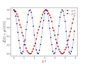
Figure 2: Oscillations of the Loschmidt probability ${\cal L}(t)=p(1111)$ for the square $\mathbb{Z}_{2}$ plaquette on the ibmq_qasm_simulator, which is a general purpose simulator. The points are the points from the simulator, and the line is only to guide the eye. The system has a two-dimensional gauge invariant Hilbert space, and there is a two-state Rabi oscillation when started from the state $|1111\rangle$ to the state $|0000\rangle$. An identical behavior is also observed in the triangular $Z(2)$ plaquette. Increasing the coupling by a factor of two is identical to speeding up the dynamics by a factor of two.

It is also possible to consider the $\mathbb{Z}_{2}$ gauge theory on different lattices, such as the triangular, hexagonal, or the checkerboard lattice. Here we will also consider the example of a triangular lattice. Again, considering a single plaquette as illustrated in Figure 1 (below), there are three links in a plaquette, and each vertex contains two links where the Gauss law can be imposed. In this case, labelling the three vertices as $A,B,$ and $C$; and the three links as $1,2,3$, the Hamiltonian and the Gauss law are:

$$\begin{split}H&=-g\leavevmode\nobreak\ S^{z}_{1}S^{z}_{2}S^{z}_{3},\\ V_{A}&=\sigma^{x}_{1}\sigma^{x}_{2};\leavevmode\nobreak\ V_{B}=\sigma^{x}_{2}\sigma^{x}_{3};\leavevmode\nobreak\ V_{C}=\sigma^{x}_{3}\sigma^{x}_{1}\,.\end{split}$$ (8)

The analysis of the triangular plaquette is also similar to the square plaquette, leading to two quantum states in each Gauss law sector (and four sectors total), and thus the real-time evolution also displays a characteristic Rabi oscillation similar to the one in the square plaquette.

In the following sections, we study both plaquette models on a quantum hardware, where decoherence will cause mixing among the different sectors. The extent of the mixing can help us to understand the (in-)efficiency of the quantum hardware, and which optimizations, error corrections or mitigations are likely to help.

II.2 The U(1) quantum link model

We next consider the case of the $U(1)$ lattice gauge theory, which has considerably richer physics; and as a stepping stone to studying QED, has relevance to the fundamental physics of Nature. We will consider the theory on both the square and the triangular lattice, as in the case of the $\mathbb{Z}_{2}$ theory. The phase diagrams of both systems have been studied in the literature [69, 67], as well as aspects of dynamics and thermalization of the model on the square lattice [70] and its potential realization on analog and digital computers [71, 72, 73]. Since we want to implement the models using actual quantum hardware, we will consider very small systems involving single and double plaquettes, as shown in Figure 3.

Figure 3: Sample basis states for the square (top) and triangular (bottom) plaquettes of the $U(1)$ QLM, where the spins are quantized in the $\sigma^{z}$ basis. For the square lattice, the spins pointing up (down) indicated by arrows on the vertical links correspond to $E=+\frac{1}{2}(-\frac{1}{2})$. For the links along the x-axis (the horizontal links), the arrows pointing to the right (left) indicate spins quantized along $E=+\frac{1}{2}(-\frac{1}{2})$. For the triangular plaquette, the arrows pointing in the clockwise (counter-clockwise) direction indicate spins quantized along the $E=+\frac{1}{2}(-\frac{1}{2})$. Each of these examples of the basis states are in the $G_{x}=0$ sector, which can be seen physically from the fact that every point has one arrow coming in and another going out.

To implement a local $U(1)$ symmetry for the Hamiltonian in a simple way, we need the spin raising and lowering operators, given by: $U_{l}=S^{+}_{l}=\frac{1}{\sqrt{2}}(\sigma^{x}_{l}+i\sigma^{y}_{l})$ and $U^{\dagger}_{l}=S^{-}_{l}=\frac{1}{\sqrt{2}}(\sigma^{x}_{l}-i\sigma^{y}_{l})$. The operators $U_{l}$ (and $U_{l}^{\dagger}$) are canonically conjugate to the electric flux operator living on the same link, $E_{l}=S^{z}_{l}$, and obey the following commutation relations:

$$[E,U]=U;\leavevmode\nobreak\ \leavevmode\nobreak\ [E,U^{\dagger}]=-U^{\dagger};\leavevmode\nobreak\ \leavevmode\nobreak\ [U,U^{\dagger}]=2E\,.$$ (9)

Operators residing on different links always commute. With these operators, we can now define the lattice $U(1)$ Gauss law:

$$G_{x}=\sum_{\mu}\left(E_{x,\mu}-E_{x-\mu,\mu}\right).$$ (10)

Note that $\mu$ denotes the lattice unit vectors, and thus for the square lattice $\mu=1,2$, while for the triangular lattice $\mu=1,2,3$. This operator $G_{x}$ generates the gauge transformations, which can be expressed as $V=\prod_{x}\exp\left(-i\alpha_{x}G_{x}\right)$, where $\alpha_{x}$ is the (local) parameter associated with the local unitary transformation. This operator commutes with the plaquette Hamiltonian defined on the entire lattice. For the square lattice, the local Hamiltonian involves four links around a plaquette, and the model has the form

$$\begin{split}H_{\Box}&=-g\sum_{\Box}\left(U_{\Box}+U^{\dagger}_{\Box}\right),\\ U_{\Box}&=S^{+}_{r,\mu}S^{+}_{r+\mu,\nu}S^{-}_{r+\nu,\mu}S^{-}_{r,\nu},\end{split}$$ (11)

where $\mu,\nu$ are the lattice axes and $r$ is the bottom left corner of a square plaquette. For the triangular lattice, the 3-link plaquette Hamiltonian has the form:

$$\begin{split}H_{\triangle}&=-g\sum_{\triangle}\left(U_{\triangle}+U^{\dagger}_{\triangle}\right),\\ U_{\triangle}&=S^{+}_{xy}S^{+}_{yz}S^{+}_{zx},\end{split}$$ (12)

where the points $x,y,z$ are the vertices of a triangle. Mathematically, the commutation relation $[G_{x},H]=0$ ensures that the Hamiltonian is invariant under local unitary transformations $H=VHV^{\dagger}$, resulting in a highly constrained system.

From these equations, the single-plaquette case can be obtained by only keeping the links that exist in the triangle or the square geometry, and gives rise to:

$$\begin{split}H_{\Box}&=-g(S^{+}_{1}S^{+}_{2}S^{-}_{3}S^{-}_{4}+S^{-}_{1}S^{-}_{2}S^{+}_{3}S^{+}_{4});\\ H_{\triangle}&=-g(S^{+}_{1}S^{+}_{2}S^{+}_{3}+S^{-}_{1}S^{-}_{2}S^{-}_{3});\\ \end{split}$$ (13)

with Gauss law operators given by

$$G_{A} =S^{z}_{4}+S^{z}_{1},\qquad G_{B}=S^{z}_{2}-S^{z}_{1}$$ (14)

$$G_{C} =-S^{z}_{2}-S^{z}_{3},\qquad G_{D}=S^{z}_{3}-S^{z}_{4},$$

for the square plaquette, and

$$G_{A}=S^{z}_{1}-S^{z}_{3},\;\;G_{B}=S^{z}_{2}-S^{z}_{1},\;\;G_{C}=S^{z}_{3}-S^{z}_{2}$$ (15)

for the triangular plaquette, where the link subscripts correspond to the labels in Figure 3. Note that the conventions for the signs of the electric flux are given in the caption of the figure.

For our purposes, it is useful to further simplify Equation (13) and express the Hamiltonian in terms of the Pauli matrices, which will allow us to construct the quantum circuits using the circuit identities introduced in the next section. For the square plaquette we obtain:

$$\begin{split}H_{\Box}&=-\frac{g}{2}\left[\sigma^{x}_{1}\sigma^{x}_{2}\sigma^{x}_{3}\sigma^{x}_{4}+\sigma^{y}_{1}\sigma^{y}_{2}\sigma^{y}_{3}\sigma^{y}_{4}-\sigma^{x}_{1}\sigma^{x}_{2}\sigma^{y}_{3}\sigma^{y}_{4}\right.\\ &\qquad\qquad\left.-\sigma^{y}_{1}\sigma^{y}_{2}\sigma^{x}_{3}\sigma^{x}_{4}+\sigma^{y}_{1}\sigma^{x}_{2}\sigma^{y}_{3}\sigma^{x}_{4}+\sigma^{y}_{1}\sigma^{x}_{2}\sigma^{x}_{3}\sigma^{y}_{4}\right.\\ &\qquad\qquad\left.+\sigma^{x}_{1}\sigma^{y}_{2}\sigma^{y}_{3}\sigma^{x}_{4}+\sigma^{x}_{1}\sigma^{y}_{2}\sigma^{x}_{3}\sigma^{y}_{4}\right].\end{split}$$ (16)

Thus there are eight terms for a single plaquette when expressed with the Pauli matrices. For the triangular plaquette, we have four independent plaquette terms which have to be implemented in a quantum circuit:

$$H_{\triangle} =-g/\sqrt{2}\left[\sigma^{x}_{1}\sigma^{x}_{2}\sigma^{x}_{3}-\sigma^{y}_{1}\sigma^{y}_{2}\sigma^{x}_{3}\right.$$ (17)

$$\left.\qquad\qquad\quad-\sigma^{y}_{1}\sigma^{x}_{2}\sigma^{y}_{3}-\sigma^{x}_{1}\sigma^{y}_{2}\sigma^{y}_{3}\right].$$

The solution of the single-plaquette problem is straightforward: for the $U(1)$ system as defined here, it is more natural to consider the system quantized in the $\sigma^{z}$-basis (instead of the $\sigma^{x}$-basis used in the $\mathbb{Z}_{2}$ case), such that the spin-up and the spin-down can be denoted by arrows pointing in and pointing out respectively from a given site. This can be interpreted physically as the plaquette operators raising or lowering states by a unit of magnetic field (which is like a clockwise or anti-clockwise arrangement of the electric fluxes around the plaquette). For the triangular lattice this means that there are only $2^{3}=8$ basis states, and the square lattice has $2^{4}=16$ such basis states. The Gauss law further selects only two basis states for each of the two lattices. For the triangular lattice with $G_{x}=0$ everywhere as an example, we denote them as $\ket{000}$ and $\ket{111}$; while for the square lattice with $G_{x}=0$ we denote them as $\ket{0011}$ and $\ket{1100}$. Note that $0$ denotes a spin-up and $1$ a spin-down in the $\sigma^{z}$ basis. The states are shown in Figure 3. The Hamiltonian for both cases is therefore a two-dimensional off-diagonal matrix. The two eigenstates are thus given by a symmetric and anti-symmetric linear superposition of the two basis states. The real-time evolution – with the Loschmidt probability oscillating between the two basis states – is qualitatively the same as that given in Figure 2, the period simply differs as a function of $g$.

II.3 Two-plaquette system

As one more test of the quantum hardware, we consider a two-plaquette system on a square lattice with periodic boundary conditions for the $\mathbb{Z}_{2}$ gauge theory. The geometry of the system is shown in Figure 4.

Figure 4: The set-up for two plaquettes which have periodic boundary conditions in the longer direction. The links are marked with numerals, while the sites are marked with letters.

For clarity, let us explicitly write the Hamiltonian and the Gauss law for this case:

$$\begin{split}H&=-gS^{z}_{1}S^{z}_{2}S^{z}_{3}S^{z}_{4}-gS^{z}_{5}S^{z}_{4}S^{z}_{6}S^{z}_{2},\\ G_{A}&=\sigma^{x}_{1}\sigma^{x}_{4}\sigma^{x}_{5};\leavevmode\nobreak\ \leavevmode\nobreak\ \leavevmode\nobreak\ \leavevmode\nobreak\ G_{B}=\sigma^{x}_{5}\sigma^{x}_{2}\sigma^{x}_{1};\\ G_{C}&=\sigma^{x}_{6}\sigma^{x}_{2}\sigma^{x}_{3};\leavevmode\nobreak\ \leavevmode\nobreak\ \leavevmode\nobreak\ \leavevmode\nobreak\ G_{D}=\sigma^{x}_{3}\sigma^{x}_{4}\sigma^{x}_{6},\end{split}$$ (18)

following the labeling in Figure 4. Because the $\sigma_{\rm N}^{z}$ commute with each other, the time evolution given by this Hamiltonian can be decomposed as the evolution given by the product of the time evolution given by each of the two terms for $H$ in Equation (18). This decomposition is exact and not subject to any Trotter errors. For each term, we can use the strategy to be described in the next section: introduce an ancillary qubit which couples to the rest of qubits in the plaquette, and perform dynamics with the help of the ancillary qubit. Further, the structure of the Gauss law implies that we can impose the constraint $G_{x}=1$ for all the sites. Without the constraint, there are $2^{6}=64$ states. The Gauss law constraint will then reduce this number. For example, imposing $G_{A}=1$ affects the spins on the links 1, 4, and 5. Only those configurations are allowed where either all three have $+1$ in the $\sigma^{x}$ basis, or exactly two of the spins 1,2, and 5 have $-1$ in the $\sigma^{x}$ basis, and the third spin is $+1$.

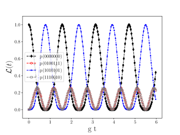
Figure 5: Quench dynamics of the two-plaquette simulation from state 1 into the states 2,3, and 4, given by the ibmq-qasm-simulator. The Loschmidt probability oscillates between 0 and 1 for the states 1 and 3, while it oscillates between 0 and 0.25 for the states 2 and 4. Moreover, the probability oscillations between state 1 and 3 are exactly out of phase, as in the two-state systems considered previously, but it has equal projections into states 2 and 4. As before, the points are the ones from the simulator, and the dashed line only guides the eye.

While the solution of the two plaquette system is worked out in Appendix B, we summarize the relevant points for the simulation of quench dynamics of this system. The two plaquette system in the sector $G_{x}=1$ for all $x$ has 8 basis states. These 8 states can be further divided into two sectors using the global winding number symmetry, which cuts the plaquettes horizontally and vertically respectively.

For a general rectangular system with sizes $L_{\rm x}\times L_{\rm y}$, we can define a global winding number $W_{n}$ for each of the spatial directions. If we draw a line at a fixed $x=x_{0}$ ($y=y_{0}$) along the $y$($x$)-direction, then this line cuts all horizontal (vertical) links (i.e. those pointing in the $x$($y$)-direction). Denoting the set of spins on the line as $\{\sigma_{m}\}$, our winding number operator is given by

$$W_{n}=\prod_{m}\sigma^{x}_{m},$$ (19)

where $n=y$ if $m=x$ and vice-versa. For our case, the expressions for the operators are

$$W_{x} =\sigma^{x}_{4}\sigma^{x}_{2};\leavevmode\nobreak\ \leavevmode\nobreak\ \leavevmode\nobreak\ W_{y}(13)=\sigma^{x}_{1}\sigma^{x}_{3};\leavevmode\nobreak\ \leavevmode\nobreak\ \leavevmode\nobreak\ W_{y}(56)=\sigma^{x}_{5}\sigma^{x}_{6}.$$ (20)

The last two expressions for $W_{y}$ are actually the same, as can be seen by using the Gauss law for the sites. Thus, in a perfect implementation, only 4 basis states entangle with each other under a unitary evolution. In Figure 5 we show the Loschmidt probability for starting in one of these states, and the oscillations into the other three states. This system thus provides a good playground for tuning quantum hardware to reproduce these involved oscillations, as well as benchmarking to what extent local and global symmetries can be preserved in these circuits.

For completeness, consider the $U(1)$ theory on two plaquettes, the entire Hamiltonian would have a total of 16 terms, which represented by the quantum gates are:

$$\begin{split}H&=-\frac{J}{2}\left[\sigma^{x}_{1}\sigma^{x}_{2}\sigma^{x}_{3}\sigma^{x}_{4}+\sigma^{y}_{1}\sigma^{y}_{2}\sigma^{y}_{3}\sigma^{y}_{4}-\sigma^{x}_{1}\sigma^{x}_{2}\sigma^{y}_{3}\sigma^{y}_{4}\right.\\ &-\sigma^{y}_{1}\sigma^{y}_{2}\sigma^{x}_{3}\sigma^{x}_{4}+\sigma^{y}_{1}\sigma^{x}_{2}\sigma^{y}_{3}\sigma^{x}_{4}+\sigma^{y}_{1}\sigma^{x}_{2}\sigma^{x}_{3}\sigma^{y}_{4}+\sigma^{x}_{1}\sigma^{y}_{2}\sigma^{y}_{3}\sigma^{x}_{4}\\ &+\sigma^{x}_{1}\sigma^{y}_{2}\sigma^{x}_{3}\sigma^{y}_{4}+\sigma^{x}_{5}\sigma^{x}_{4}\sigma^{x}_{6}\sigma^{x}_{2}+\sigma^{y}_{5}\sigma^{y}_{4}\sigma^{y}_{6}\sigma^{y}_{2}-\sigma^{x}_{5}\sigma^{x}_{4}\sigma^{y}_{6}\sigma^{y}_{2}\\ &-\sigma^{y}_{5}\sigma^{y}_{4}\sigma^{x}_{6}\sigma^{x}_{2}+\sigma^{y}_{5}\sigma^{x}_{4}\sigma^{y}_{6}\sigma^{x}_{2}+\sigma^{y}_{5}\sigma^{x}_{4}\sigma^{x}_{6}\sigma^{y}_{2}\\ &+\left.\sigma^{x}_{5}\sigma^{y}_{4}\sigma^{y}_{6}\sigma^{x}_{2}+\sigma^{x}_{5}\sigma^{y}_{4}\sigma^{x}_{6}\sigma^{y}_{2}\right].\end{split}$$ (21)

These terms do not all commute with each other, so trotterization would be necessary to simulate their real-time evolution. In this paper, we only consider the $\mathbb{Z}_{2}$ case which involves no Trotter steps.

III Quantum Hardware and Circuits

In our plaquette model simulations, we make use of IBM Q hardware, which is based on superconducting (transmon) qubits. We discuss below a few details on how we work with this NISQ hardware, both in terms of selecting the platform for each experiment and in terms of circuit implementation.

III.1 Hardware Selection

Superconducting qubits have the advantage of being relatively fast at running experiments compared to trapped-ion qubits, but a disadvantage of relatively short decoherence times[74].

Because of this, the topology of the circuits is important, as it will make a difference for how many gates are necessary to realize a particular simulation. Figure 6 shows three real-hardware topologies that are used in this paper. For each experiment, we may select hardware depending on optimal topology.

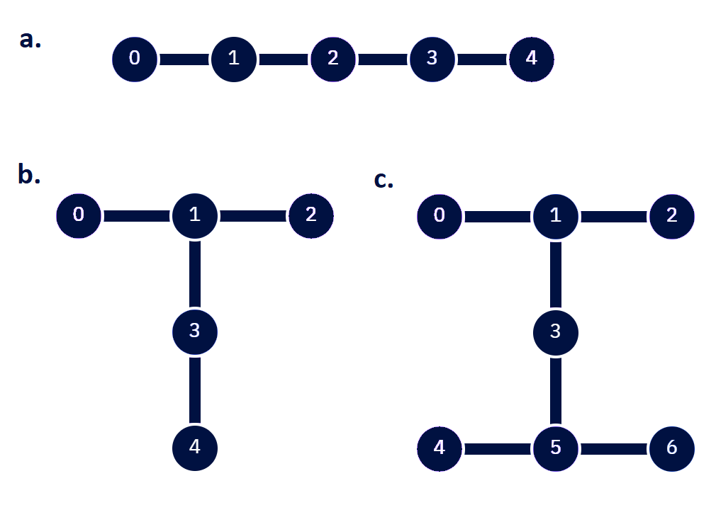
Figure 6: Three circuit topologies used for the simulations. Images taken from IBM Quantum Experience.

Another important consideration for choosing hardware is the quantum volume of the device, which is generally a measure of the most complex circuit that can compute accurate quantities according to a particular threshold for a given device. IBM Q measures quantum volume using the following formula,

$$V_{Q}=2^{{\rm min}(d,m)},$$ (22)

where $d$ is the depth of the circuit (measured according to two-qubit gates), and $m$ is the number of qubits, so that ${\rm min}(d,m)$ tells us the largest square circuit possible that still meets the set accuracy threshold [75]. The IBM Q devices each have a $V_{Q}$ measured and so in our experiments we favor using those with the higher $V_{Q}$ values. Specifically, the devices used to obtain our results include IBM Q Valencia and IBM Q Quito, which each have $V_{Q}=16$, as well as IBM Q Bogota, IBM Q Santiago, and IBM Lagos, which each have $V_{Q}=32$.

III.2 Circuit Implementation and Scaling

The real-time simulation of plaquette dynamics involves realizing Hamiltonians of several spins on a plaquette. A very simple case looks like

$$H_{\rm N}=-g\sigma^{3}_{xy}\sigma^{3}_{yz}\sigma^{3}_{zw}\sigma^{3}_{wx},$$ (23)

with ${\rm N}=4$ and the sites ${x,y,z,w}$ are corners of a square plaquette. To realize a real-time evolution with the above Hamiltonian, we implement the following gate sequence [61, 62]

$$U_{\rm S,A}(t) =\exp\left[i\frac{\pi}{4}\sigma^{3}_{\rm A}\sum_{j=1}^{N}\sigma^{3}_{j}\right]\exp\left[igt\sigma^{1}_{\rm A}\right]$$ (24)

$$\qquad\qquad\times\exp\left[-i\frac{\pi}{4}\sigma^{3}_{\rm A}\sum_{j=1}^{N}\sigma^{3}_{j}\right].$$

A proof for Equation 24 is detailed in Appendix A.

This identity has the nice property of being applicable to plaquettes that contain a general number of spins, $N$, and in all cases allows for the time-evolution portion to be done entirely on a single extra spin, which we label with the index $A$. This spin is in addition to the $N$ spins that make up the plaquette, and is known as ancillary. In principle for a quantum circuit implementation (where we represent each spin with a qubit), one would only need one ancillary qubit for the entire system, but due to topological issues it may be more efficient in terms of circuit depth to add more ancillary qubits in systems with more plaquettes. Still, with at most one ancillary qubit per plaquette, the number of qubits needed for simulation scales linearly with the number of links in the system.

If all terms in the Hamiltonian commute, the number of gates needed is constant as a function of real time, but in the more generic case where the terms do not commute and so trotterization is necessary, the circuit depth scales linearly with time. In our examples below we focus only on cases where no trotterization is needed.

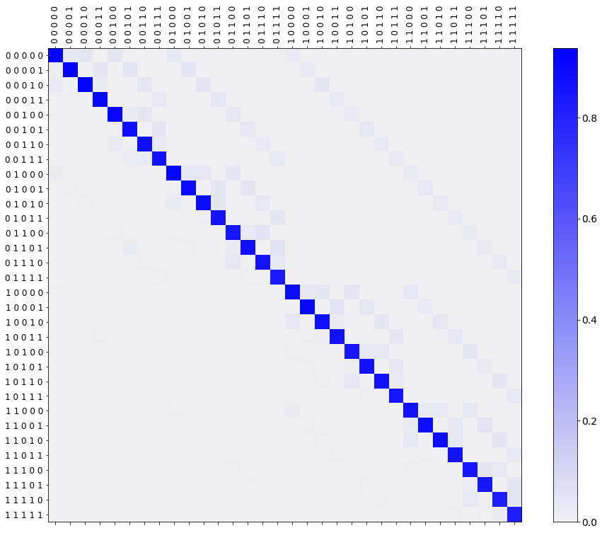
Figure 7: Response mitigation matrix computed by ignis for IBM Q Manila (5 qubit system).

IV Error Mitigation methodologies

As mentioned earlier, one major practical obstacle to develop physical devices to perform quantum computations is the significant inherent noise that affects NISQ quantum devices. In theory, quantum error correction is possible by encoding the information of the desired circuit into a highly-entangled state composed of a very large number of physical qubits [41, 42]. However, this large number of qubits makes the hardware requirements too demanding to be implemented in practice (although promising results point in the right direction [76]). An alternative is to take advantage of systematic and reproducible properties of the hardware. These properties are exploited as part of the so-called error mitigation schemes, which have proven to be successful in NISQ era devices [43, 44, 45, 46, 47, 48, 49, 51, 52, 53, 77]. Among those, we consider two types, readout error mitigation and zero noise extrapolation (ZNE); which aim to reduce noise coming from two different sources: readout and gate operation decoherence. We emphasize that while here we use these techniques on IBM Q hardware, they are in fact hardware-agnostic techniques – they rely only on the set of gates available and do not rely on the details of the hardware such as the type of qubits used–and therefore can be used to improve results on any universal quantum device.

IV.1 Readout error mitigation

One important source of errors are the so called “readout” errors, which arise due to the comparable measurement and decoherence times [51, 78, 53, 52]. This can cause undesired state decays, affecting the state captured in the measurement. Assuming a classical stochastic model for the noise affecting measurements, the statement of the problem can be formulated by using the response matrix $P(m|t)$, which connects a noisy measurement $m$ to the true/ideal measurement $t$ by the relation $m=Pt$. Naively one can use the inverse of the response matrix to obtain $t=P^{-1}m$ and recover the true value of the measurement. The problem then consists in performing a series of calibration experiments to measure $P$, and then use it to recover $t$ given $m$ in subsequent independent experiments.

Packages such as qiskit-ignis [79] are based on the response matrix formulation of the readout error mitigation scheme, but (by default) do not try to compute $P^{-1}$ directly by matrix inversion. Instead, $t$ is recovered by finding the minimum of the least squares expression:

$$f(t)=\sum_{i=1}^{2^{n}}\left(m_{i}-\left(P\cdot t\right)_{i}\right)^{2}\,,$$ (25)

where $n$ is the total number of qubits in the circuit. This methodology is more robust than matrix inversion for general NISQ hardware [79, 52]. More involved methods combine the previous approach with gate inversion to further improved the error mitigation results [53]; while unfolding methods have also been proposed and tested in the literature [52].

In most cases, the ability to apply readout error mitigation is limited by the number of qubits ($n$) in the circuit, as the number of calibration experiments required to evaluate $P$ grows as $2^{n}$. Moreover, the calibration step of estimating $P$ is hardware dependent and needs to be performed immediately before running the experiments to guarantee temporal deviations in the particular hardware are accounted for. An real-hardware example of the response matrix obtained for a 5 qubit system (IBM Q Manila) using ignis is shown in 7. As expected, the diagonal entries have probability values close to 1, but there is still significant drift towards non-diagonal entries. As presented and discussed in Sec V, correcting for these small deviations resulted in significant improvements in the final mitigated data.

Clearly, going beyond circuits with a small number of qubits would be prohibitively expensive due to the number of experiments required to evaluate the response matrix. Some proposals have considered the possibility of assuming close to uncorrelated readout errors between the qubits, which would drastically reduce the number of experiments required [78]. Studying these potential improvements goes beyond the scope of this work.

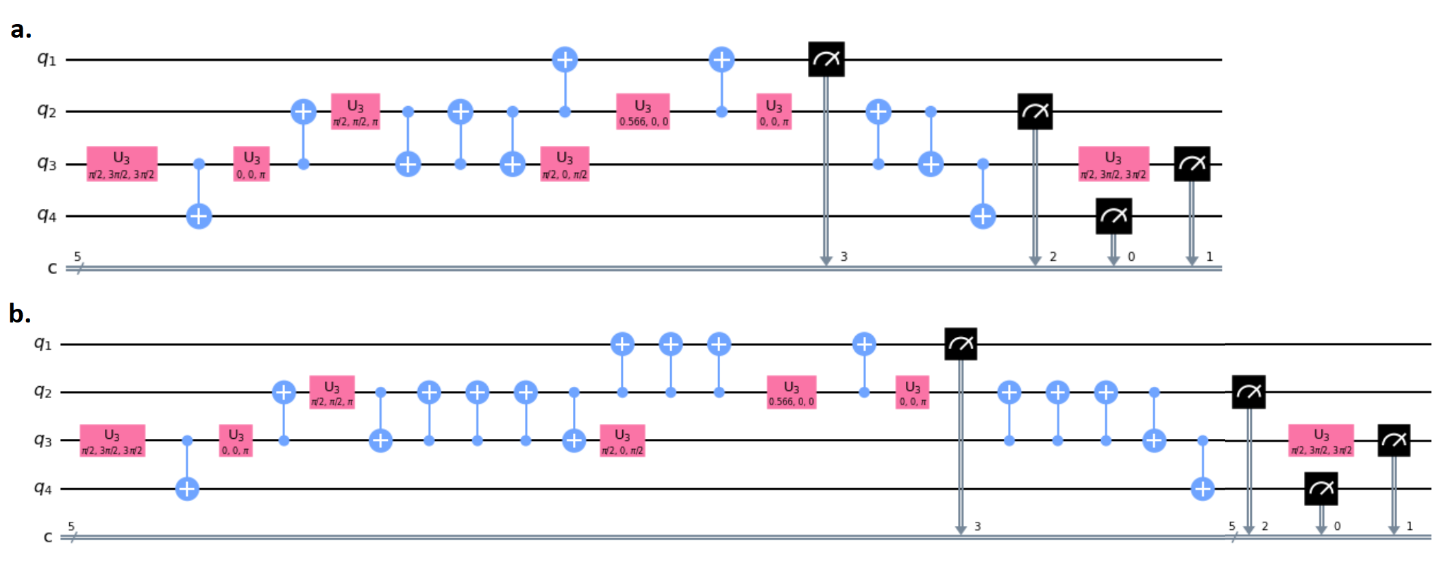
Figure 8: An example of using the Mitiq package for folding a circuit that gives the time evolution of the $Z(2)$ gauge theory on a triangular plaquette. Both circuits are equivalent, but the second one contains additional identity insertions of CNOT gates such that when measured using the CNOT circuit depth the second circuit is 1.6 times longer than the former.

IV.2 Corrections against decoherence – Mitiq

The second source of error comes from the gate portion of the circuit before measurements occur. Longer circuits will consist of more gates, and both the longer runtimes and the gate implementation (transmon qubits in the case of the IBM Q devices) will cause additional errors to pile up. To mitigate this source of error we use a method known as zero-noise extrapolation (ZNE), where we introduce additional noise in a controlled way in order to empirically develop a noise model that we can extrapolate to the zero noise case.

Implementations of ZNE include those that involve pulse control and run multiple experiments with pulses of different durations [44], and those that involve folding, which consists of insertions of additional gate identities to the circuit which would not change the results in an ideal simulation, but will make results on real hardware more noisy. This information on how the gates affect the noise level can then be used to develop a noise model and extrapolate back to an “ideal” result.

We used the folding option in this paper and specifically we used the Mitiq package to implement it [46]. As an example, Figure 8 shows two equivalent circuits, but the second circuit has three extra identity insertions, each consisting of two identical CNOT gates in a row. Because the error rates of the two-qubit CNOT gates are significantly higher than those for the single qubit gates (roughly ten times different on IBM Q devices), we will assume perfect fidelities for the single qubit gates and model all the error coming from the two-qubit gates (an option within Mitiq). With this in mind, because circuit $a$ in Figure 8 has ten CNOT gates, and circuit $b$ has sixteen CNOT gates, the scale factor of the circuit $b$ is 1.6 times that of circuit $a$.

Figure 9 shows real-hardware examples of different extrapolations for several circuits with the ideal result for each (determined using a simulator) marked at scale factor “0”. The first row shows example extrapolations for $\mathbb{Z}_{2}$ model on the square plaquette, at two different times in the evolution. The bottom left image shows an extrapolation at $t=0$ for the $\mathbb{Z}_{2}$ theory on the triangular plaquette, and the bottom right image shows one at $t=0$ for the U(1) theory on the square plaquette. The two extrapolations shown are a quadratic fit and a Richardson extrapolation, explained in Kandala et. al.[44] From this empirical data we decided to use the quadratic extrapolation for our data, as it appeared less susceptible to experimental outliers (such as those in the bottom left of Figure 9).

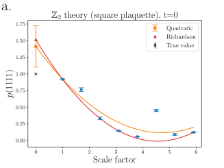
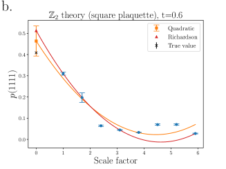
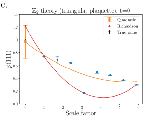
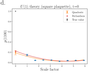
Figure 9: The plots in the top row show zero-noise extrapolation for the $\mathbb{Z}_{2}$ theory on a square plaquette (IBM Q Valencia hardware) at two times: $t=0$ ($a$) and $t=0.6$ ($b$). The bottom row shows zero-noise extrapolation for the $\mathbb{Z}_{2}$ gauge theory on a triangular plaquette (IBM Q Bogota) at $t=0$ ($c$) and a U(1) gauge theory on a square plaquette (IBM Q Quito) at $t=0$ ($d$).

It is interesting to note the presence of two regimes which display sensitivity to a change in the circuit depth. For larger scale factors which exceed the quantum volume of the system, the dependence on the scale factor becomes insensitive. At $t=0$, the measurements for increasing the circuit length decay only slowly until the scale factors exceed $3$ for the $\mathbb{Z}_{2}$ model, and about $6$ for the $U(1)$ model. For $t=0.6$ this decay is much faster for the $U(1)$ model than the $\mathbb{Z}_{2}$ model. Typically the $U(1)$ circuit is significantly more entangled, and becomes more so when the extrapolation is attempted at finite $t$.

V Results

This section gives our real-time evolution results for the Loschmidt probability, as well as observables $G_{x}$ and $W_{y}$ for plaquette simulations on NISQ hardware. In each simulation, we take five measurements (8192 shots per measurement) at every point in time and at each of the eight different scale factors illustrated by Figure 9. This allows us to get error bars and perform ZNE at every time. For each time, the different scale factor measurements were all taken within the same calibration: see Appendix D for a note about the fluctuations of the measurements across different calibrations of the IBM Q hardware. Each simulation consists of 20 points in time total, leading to $5\times 8\times 20=800$ circuit measurements to produce the error-mitigated plots for a theory on a particular plaquette.

V.1 $\mathbb{Z}_{2}$ Theory on Single Plaquettes

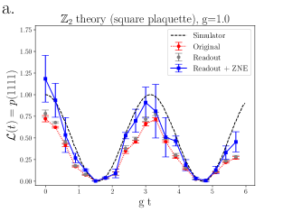
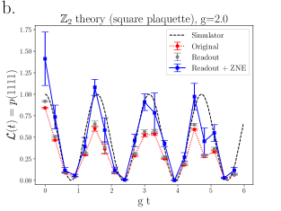
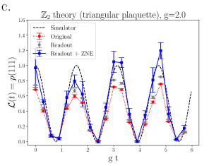
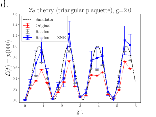
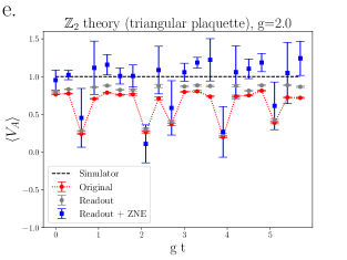
Figure 10: Real-time evolution of the $\mathbb{Z}_{2}$ theory on a single plaquette. Plots $a$ and $b$ in the first row show the Loschmidt probability data for a square plaquette on IBM Q Valencia (with two couplings: g=1.0,2.0), then plots $c$ and $d$ show the Loschmidt probability data for a triangular plaquette on IBM Q Bogota. Finally, plot $e$ shows the Gauss law observable $V_{A}$, which means the observable involving the links 1 and 2, as shown in Figure 1.

We first discuss the results for the $\mathbb{Z}_{2}$ theory on square and triangular plaquettes, which were simulated on IBM Q Valencia and IBM Q Bogota, respectively. The results are plotted in Figure 10. The plots $a$ and $b$ in the top row of the figure show a simulation of a single square plaquette system for two different couplings: $g=1.0$ and $g=2.0$. We chose IBM Q Valencia for this simulation because of its T-shaped topology, illustrated in $b$ of Figure 6, which reduced the circuit depth necessary since the ancillary qubit could be placed at a junction directly connected to three other qubits. There was other hardware available with better $V_{Q}$ (32 versus 16 for Valencia), but the topological advantage of the T-shaped hardware made for better results despite the worse $V_{Q}$. In these plots we give the ideal simulator measurement of the Loschmidt probability in addition to the original (raw) data from the circuit, followed by the readout error correction, followed by the readout and ZNE error corrections in combination. Here we see that with both these corrections we are able to get to the correct simulator measurements within errors.

The next two plots, $c$ and $d$ in the bottom row of Figure 10 give the results for a $\mathbb{Z}_{2}$ theory on a triangular plaquette instead. Here a smaller circuit depth is needed as compared to the square plaquette, so we use IBM Q Bogota due to its better quantum volume (it has a linear topology, as seen in $a$ in Figure 6). These plots give the time-evolution for the two states in the $V_{A}=V_{B}=V_{C}=1$ sector: $\left|000\right\rangle$ and $\left|111\right\rangle$, and one can see from the simulator lines that their probabilities always add up to 1. As in the case for the $\mathbb{Z}_{2}$ theory on the square plaquette, the error mitigation methods allow for the fully mitigated data to track the simulator data within error bars. The last plot $e$ in the lower right corner of Figure 10 is a measure of how well the circuits for the system on the triangular plaquette are producing only states that have $V_{A}=1$. It shows measurements throughout the time evolution of $\left\langle V_{A}\right\rangle$, and as the simulator line shows, ideally it would remain exactly equal to 1 throughout the time evolution. The mitigated measurements show how for most time measurements we are able to produce $\left\langle V_{A}\right\rangle=1$ within error bars.

We further note that the circuit depths for the simulations of the $\mathbb{Z}_{2}$ theory on the square plaquette lead to circuit volumes clearly greater than the quantum volume $V_{Q}$ measurements of the quantum hardware ($d=8$, $m=5$ leading to a circuit volume of $40$ for the square plaquette, whereas $V_{Q}$ is 16 on IBM Q Valencia–suggesting a maximum square circuit volume of $16$, with $d=m=4$.) The simple mitigation techniques employed thus seem to allow us to “beat” the quantum volume limitations for the hardware and get results consistent with the simulator within errors. For the triangular plaquette on IBM Q Bogota, we have $d=8$, $m=4$, leading to a circuit volume of $32$, whereas the $V_{Q}$ of the hardware is $32$, corresponding to a $d=m=5$ square. It is less clear whether we have exceeded quantum volume limitations for this simulation, and indeed empirically most Loschmidt probability data seems to meet the IBM Q threshold of $67\%$ of the ideal amplitude[75], but again we see that our mitigation efforts are successful at restoring the full measurement values.

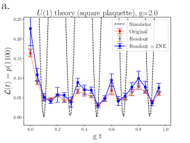
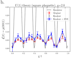
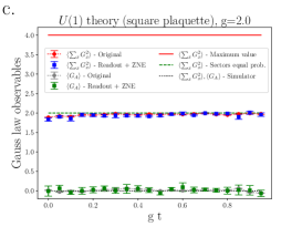
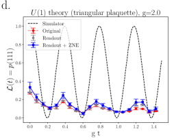
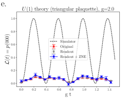
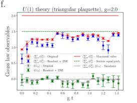
Figure 11: Real-time evolution of the $U(1)$ theory on a single plaquette. The top row shows results for the square plaquette on IBM Q Quito hardware, with plots $a$ and $b$ showing Loschmidt probability data, and then plot $c$ showing different Gauss law observables $G_{A}$ and $\sum_{x}G_{x}^{2}$, with $G_{x}$ defined in Equation (10). The bottom row shows results for the triangular plaquette on IBM Q Manila hardware, with again the first two plots $a$ and $b$ showing Loschmidt probability data, and the third showing the $G_{A}$ and $\sum_{x}G_{x}^{2}$ Gauss law observables.

V.2 $U(1)$ Theory on Single Plaquettes

We next present the data for the $U(1)$ theory on a single square plaquette and a single triangular plaquette, which we ran on IBM Q Quito and IBM Q Manila, respectively. Similar to the $\mathbb{Z}_{2}$ case, IBM Q Quito has a T-shaped architecture (as seen in $b$ of Figure 6) with $V_{Q}=16$, while IBM Q Manila has a linear topology (as seen in $a$ of Figure 6) with $V_{Q}=32$. We ran the square plaquette simulation on the T-shaped architecture because despite its lower $V_{Q}$, the topological advantages requiring fewer two-qubit gates made for better data. Indeed, we could not get any signal at all for the square plaquette $U(1)$ model on current linear-topology IBM Q devices.

Figure 11 shows the data for the $U(1)$ simulations. The first row of plots gives the square plaquette simulation data, with the first two plots $a$ and $b$ showing Loschmidt probability data for the two states $\left|1100\right\rangle$ and $\left|0011\right\rangle$ in the $G_{x}=0$ sector. Here we are running circuits that have much greater volume than the quantum volume limitations, with $m=5$ and $d=80$, and so we cannot come close to the correct amplitudes of the oscillations (shown by the dashed simulator lines), but we are able to make out some oscillations and see some qualitative similarity between the experimental data and the simulator data. It is clear however that the folding ZNE is unable to improve the accuracy of the data at this level.

The last plot $c$ in the top row is a test of how well the time-evolved system stays in the $G_{x}=0$ sector by measuring two quantities: $G_{A}$ in particular and then $\sum_{x}G_{x}^{2}$. For both of these quantities we would expect to get zero in the ideal case, and indeed the data for $G_{A}$ stays quite close to zero. As this is a simple average of $G_{A}$ however, we cannot rule out that many $G_{A}$ measurements of $+1$ and $-1$ also exist in roughly equal quantities and are being averaged away, and indeed the leakage seen from the other plots suggests this must be occurring. We can quantify this leakage better by additionally measuring $\sum_{x}G_{x}^{2}$, which ideally should also be equal to $0$ at all times. Here we also plot two lines: one at $4$, which is the maximum value one could possibly get (by staying in the $G_{x}=\pm 1$ sectors, because the observable would be $4\times(\pm 1)^{2}=4$), and one at $2$, which is the value one would get if all sectors were equally represented in the time-evolution (for the sixteen sectors average we would get $(2\times 0+12\times 2+2\times 4)/16=2$). When we look at our experimental data we see that indeed the measurements are quite close to all sectors being equally likely, but they are mostly slightly below that line. This suggests a slight bias toward the $G_{x}=0$ sector.

The second row of Figure 11 shows the data for the $U(1)$ theory on the triangular plaquette, with the first two plots $d$ and $e$ giving the Loschmidt probability for states $\left|000\right\rangle$ and $\left|111\right\rangle$, which are the two states in the $G_{x}=0$ sector. Again with $d=4$ and $m=40$ we are likely far past the volume threshold suggested by $V_{Q}=32$, and indeed the original data never comes close to the maximum amplitudes of $1$ in the oscillations. However, again we are able to make out a qualitative agreement in behavior. We also see a close agreement in the frequency of the oscillations and that ZNE does still incrementally improve the results, unlike in the square plaquette case.

The last plot $f$ in the bottom row again measures $G_{A}$ and $\sum_{x}G_{x}^{2}$, and again the $G_{A}$ observable is mostly close to $0$, but once more, this can be explained by “leaky” states in both $G_{A}=1$ and $G_{A}=-1$ sectors also being sampled (so long as both the $G_{A}=1$ and $G_{A}=-1$ errors are equally likely). We see this more clearly by measuring $\sum_{x}G_{x}^{2}$ as well. Again we show two lines for comparison: the “maximum value” line shows the case where we get the largest value for the triangular plaquette, which occurs when $G_{x}=\pm 1$ for two of the sites and $G_{x}=0$ for the third site. This results in an average value of $2$, and we see our experimental values are well below that. The second line again shows the value we would get if all sectors in the time evolution were equally likely (obtained by computing $(2\times 0+6\times 2)/8=3/2$ for the eight sectors of the triangular plaquette system). Here we see quite clearly that even though our experimental data for $\sum_{x}G_{x}^{2}$ is much larger than $0$, it is also clearly smaller than $3/2$, indicating a clear bias toward the $G_{x}=0$ sector.

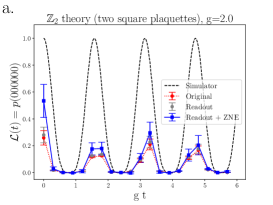
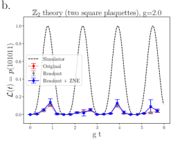
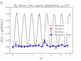
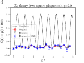
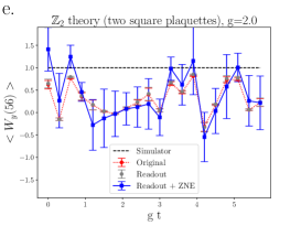
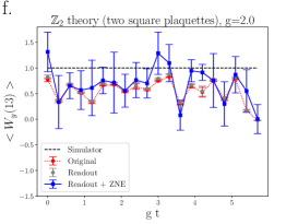
Figure 12: Plots for the two-plaquette $\mathbb{Z}_{2}$ system, which was run on IBM Lagos. The first two plots $a$ and $b$ give the Loschmidt probabilities for states $\left|000000\right\rangle$ and $\left|101011\right\rangle$ which oscillate between $0$ and $1$, and the next two plots $c$ and $d$ give the Loschmidt probabilities for states $\left|010111\right\rangle$ and $\left|111100\right\rangle$, which oscillate between $0$ and $0.25$. The last two plots $e$ and $f$ are for the winding number observables in the $y$-direction, the first involving links 5 and 6, and the second involving links 1 and 3, as defined in Figure 4.

V.3 $\mathbb{Z}_{2}$ Theory: Two-plaquette System

Finally we turn to the time-evolution of the $\mathbb{Z}_{2}$ theory on the two-square-plaquette system, whose ideal behavior was shown in Figure 5, where we see that if the system’s initial state is in the sector where $G_{x}=1$, the system’s evolution involves only the four states that fall into that sector. As illustrated by Figure 4, we are using periodic boundary conditions, and so there are six distinct links in the two-square-plaquette system. With the addition of an ancillary qubit, that brings us to seven qubits minimum for our simulation, and so we used the seven-qubit IBM Lagos device to obtain real-time dynamics data.

Figure 12 gives the results for the simulation, with the first four plots $a$-$d$ giving Loschmidt probability data for the four states in the $G_{x}=1$ sector; which we label $\left|000000\right\rangle$, $\left|101011\right\rangle$, $\left|010111\right\rangle$, and $\left|111100\right\rangle$ in reference to the numbered links in Figure 4. The $V_{Q}=32$ for IBM Lagos tells us that the maximum square circuit meeting the accuracy threshold is $5\times 5$. Comparing that to the two plaquette system circuit requirement with $m=7,d=48$ indicates that we are way beyond the quantum volume limit. However, especially for the states $\left|000000\right\rangle$ and $\left|101011\right\rangle$; where the simulator shows us the maximum amplitude goes up to $1$, we are able to see qualitative agreement and the readout error and ZNE error corrections do provide incremental improvements to the results.

The last two plots $e$ and $f$ give data for the winding number observable $W_{y}$, defined in Equation 20. As noted from before, the winding number in the $y$-direction can be measured using links 1 and 3 as well as links 5 and 6, and in each case the result should be the same throughout the time-evolution for the initial conditions that we chose: $W_{y}=1$. Indeed when we take the data and use ZNE, we do see a bias in the data closer to $+1$ than $-1$ for both $W_{y}$ observables. As discussed in the section II, the winding number is a topological quantity, which is dependent on how the spins along a line spanning the entire system behaves. It is thus expected that this quantity could be robust against decoherence noise. In fact, our results here qualitatively confirm this, since we see that the winding number expectation value stays close to the winding number sector that the initial state belonged to. Of course, one needs to verify this on larger circuits.

VI Conclusions

In this paper we have explored the possibilities for real-time simulations of plaquette theories on current NISQ hardware, including theories with $\mathbb{Z}_{2}$ symmetries as well as the $U(1)$ symmetry, which is of particular interest from the QED perspective. We find that for the $\mathbb{Z}_{2}$ single plaquette models, we can successfully overcome quantum volume, $V_{Q}$, limitations with the error mitigation schemes of readout error mitigation as well as ZNE through circuit folding. In cases where the circuit significantly exceeds the quantum volume, such as the cases of the two-plaquette $\mathbb{Z}_{Z}$ model and the $U(1)$ models, the error mitigation does not have a significant effect on the results. However, since the error mitigation techniques used are hardware agnostic, this has promising implications for NISQ devices in general, rather than only on IBM Q devices. Even in cases where we cannot overcome $V_{Q}$ limitations, we are still able to see qualitative signals of the real-time dynamics for circuits that are many times deeper than the $V_{Q}$ measurements for the hardware. We have seen that topology is also an important consideration for quantum simulations with superconducting qubits in particular, and found significant quantitative advantages in choosing the best topology for each experiment.

Future improvements specific to superconducting qubits would involve using pulse control for ZNE rather than folding, as well as denser data points to capture the time evolution for a plaquette model. Additionally, future work could involve simulating the real-time dynamics of non-Abelian plaquette models. Another immediate attempt would be to use different encoding strategies already with the microscopic model. For example, the $U(1)$ or the $\mathbb{Z}_{2}$ models can be represented in terms of dual height variables in 2-spatial dimensions, which already removes much of the gauge non-invariant states. Formulating quantum circuits on the dualized versions of such models would enable bigger lattices to be realized on quantum circuits [67]. Similarly, the use of rishons allows a gauge invariant formulation of several non-Abelian gauge theories such as the aforementioned $SO(3)$-symmetric model, which can then be used to construct quantum circuits on NISQ devices [80, 60].

Appendix A Proof of circuit identity

Let us label $S^{3}_{\rm N}=\sum_{j=1}^{N}\sigma^{3}_{j}$. Using this definition, we want to prove

$$U_{\rm S,A}(t)= \exp\left[i\frac{\phi}{2}\sigma^{3}_{\rm A}S^{3}_{\rm N}\right]\exp\left[igt\sigma^{1}_{\rm A}\right]$$ (26)

$$\qquad\times\exp\left[-i\frac{\phi}{2}\sigma^{3}_{\rm A}S^{3}_{\rm N}\right].$$

The physics behind the implementation is that the real-time evolution is performed on a single qubit, called the ancillary qubit. However, before and after, the ancillary qubit is entangled with the ${\rm N}$ qubits, so that the required dynamics is also induced on them.

To prove the relation, we first note,

$$\sigma^{1}_{\rm A}\exp\left[i\frac{\phi}{2}\sigma^{3}_{\rm A}S^{3}_{\rm N}\right]=\exp\left[-i\frac{\phi}{2}\sigma^{3}_{\rm A}S^{3}_{\rm N}\right]\sigma^{1}_{\rm A}.$$ (27)

This relation can be obtained by expanding the exponential and noting that $\sigma_{\rm A}$ commutes with all the other $\sigma_{j}$, and satisfies the following anti-commutation relations

$$\{\sigma^{\alpha}_{\rm A},\sigma^{\beta}_{\rm A}\}=2\delta^{\alpha\beta}.$$ (28)

We then commute the $\sigma^{1}_{\rm A}$ across at the expense of a negative sign in the series, and then re-exponentiating it, proves the relation 27.

Thus:

$$\begin{split}U_{\rm S,A}(t)&=\exp\left[i\frac{\phi}{2}\sigma^{3}_{\rm A}S^{3}_{\rm N}\right]\left[{\rm cos}(gt)-i{\rm sin}(gt)\sigma^{1}_{\rm A}\right]\\ &\qquad\times\exp\left[-i\frac{\phi}{2}\sigma^{3}_{\rm A}S^{3}_{\rm N}\right]\\ &={\rm cos}(gt)-i{\rm sin}(gt)\sigma^{1}_{\rm A}\exp\left[-i\phi\sigma^{3}_{\rm A}S^{3}_{\rm N}\right]\end{split}$$ (29)

Next, we note that

$$(\sigma^{1}_{\rm A} \exp\left[-i\phi\sigma^{3}_{\rm A}S^{3}_{\rm N}\right])^{n}$$ (30)

$$\qquad\qquad=\left\{\begin{array}[]{cc}1,&\;n\;{\rm even}\\ \sigma^{1}_{\rm A}\exp\left[-i\phi\sigma^{3}_{\rm A}S^{3}_{\rm N}\right],&\;n\;{\rm odd}\end{array}\right.$$

For $n=2$,

$$(\sigma^{1}_{\rm A}\exp\left[-i\phi\sigma^{3}_{\rm A}S^{3}_{\rm N}\right])(\sigma^{1}_{\rm A}\exp\left[-i\phi\sigma^{3}_{\rm A}S^{3}_{\rm N}\right])$$

$$\qquad\qquad=(\sigma^{1}_{\rm A})^{2}\exp\left[i\phi\sigma^{3}_{\rm A}S^{3}_{\rm N}\right]\exp\left[-i\phi\sigma^{3}_{\rm A}S^{3}_{\rm N}\right]=1.$$

Similarly, for $n=3$,

$$(\sigma^{1}_{\rm A}\exp\left[-i\phi\sigma^{3}_{\rm A}S^{3}_{\rm N}\right])(\sigma^{1}_{\rm A}\exp\left[-i\phi\sigma^{3}_{\rm A}S^{3}_{\rm N}\right])$$

$$\qquad\qquad\times(\sigma^{1}_{\rm A}\exp\left[-i\phi\sigma^{3}_{\rm A}S^{3}_{\rm N}\right])$$

$$=(\sigma^{1}_{\rm A})^{2}\exp\left[i\phi\sigma^{3}_{\rm A}S^{3}_{\rm N}\right]\exp\left[-i\phi\sigma^{3}_{\rm A}S^{3}_{\rm N}\right]$$

$$\qquad\qquad\times(\sigma^{1}_{\rm A}\exp\left[-i\phi\sigma^{3}_{\rm A}S^{3}_{\rm N}\right])$$

$$=(\sigma^{1}_{\rm A}\exp\left[-i\phi\sigma^{3}_{\rm A}S^{3}_{\rm N}\right]).$$

and hence the case for general $n$ follows. Then, we can re-exponentiate to give

$$\begin{split}U_{\rm S,A}&(t)={\rm cos}(gt)-i{\rm sin}(gt)\sigma^{1}_{\rm A}\exp\left[-i\phi\sigma^{3}_{\rm A}S^{3}_{\rm N}\right]\\ &=\exp\left[-igt\sigma^{1}_{\rm A}\exp\{-i\phi\sigma^{3}_{\rm A}S^{3}_{\rm N}\}\right]\\ &=\exp\left[-igt\sigma^{1}_{\rm A}\prod_{j=1}^{N}({\rm cos}(\phi)-i\sigma^{3}_{\rm A}\sigma^{3}_{j}{\rm sin}(\phi))\right]\end{split}$$ (31)

For $\phi=\frac{\pi}{2}$ (and hence the factor $\frac{\pi}{4}$ in Equation 24, we get

$$U_{\rm S,A}(t)=\exp\left[-igt\sigma^{1}_{\rm A}\prod_{j=1}^{N}(-i\sigma^{3}_{\rm A}\sigma^{3}_{j})\right]$$ (32)

For $N=1$,

$$U_{\rm S,A}(t) =\exp\left[-igt\sigma^{1}_{\rm A}(-i\sigma^{3}_{\rm A}\sigma^{3}_{1})\right]$$ (33)

$$=\exp\left[igt\sigma^{2}_{\rm A}\sigma^{3}_{1}\right]$$

For $N=2$,

$$U_{\rm S,A}(t) =\exp\left[-igt\sigma^{1}_{\rm A}(-i\sigma^{3}_{\rm A}\sigma^{3}_{1})(-i\sigma^{3}_{\rm A}\sigma^{3}_{2})\right]$$ (34)

$$=\exp\left[igt\sigma^{1}_{\rm A}\sigma^{3}_{1}\sigma^{3}_{2}\right]$$

For $N=3$,

$$U_{\rm S,A}(t) =\exp\left[(-i)^{4}gt\sigma^{1}_{\rm A}(\sigma^{3}_{\rm A}\sigma^{3}_{1})(\sigma^{3}_{\rm A}\sigma^{3}_{2})(\sigma^{3}_{\rm A}\sigma^{3}_{3})\right]$$ (35)

$$=\exp\left[-igt\sigma^{2}_{\rm A}\sigma^{3}_{1}\sigma^{3}_{2}\sigma^{3}_{3}\right]$$

For $N=4$,

$$U_{\rm S,A}(t)$$ (36)

$$\;=\exp\left[(-i)^{5}gt\sigma^{1}_{\rm A}(\sigma^{3}_{\rm A}\sigma^{3}_{1})(\sigma^{3}_{\rm A}\sigma^{3}_{2})(\sigma^{3}_{\rm A}\sigma^{3}_{3})(\sigma^{3}_{\rm A}\sigma^{3}_{4})\right]$$

$$\;=\exp\left[-igt\sigma^{1}_{\rm A}\sigma^{3}_{1}\sigma^{3}_{2}\sigma^{3}_{3}\sigma^{3}_{4}\right]$$

From $N=5$, the pattern repeats itself.

A.1 Two-qubit gate combination identity

The previous identity shows us that we need to find a way to express

$$e^{-i(\phi/2)\sigma^{z}_{1}\sigma^{z}_{i}}$$ (37)

using two-qubit gates. Using the basis $00,01,10,11$, this two-qubit gate is given by

$$\left(\begin{array}[]{cccc}e^{-i\phi/2}&0&0&0\\ 0&e^{i\phi/2}&0&0\\ 0&0&e^{i\phi/2}&0\\ 0&0&0&e^{-i\phi/2}\end{array}\right).$$ (38)

We can get this gate, up to a constant, using

$$e^{-i\phi/2\sigma^{z}_{1}} =\left(\begin{array}[]{cccc}e^{-i\phi/2}&0&0&0\\ 0&e^{-i\phi/2}&0&0\\ 0&0&e^{i\phi/2}&0\\ 0&0&0&e^{i\phi/2}\end{array}\right),$$ (39)

$$e^{-i\phi/2\sigma^{z}_{i}} =\left(\begin{array}[]{cccc}e^{i\phi/2}&0&0&0\\ 0&e^{-i\phi/2}&0&0\\ 0&0&e^{i\phi/2}&0\\ 0&0&0&e^{-i\phi/2}\end{array}\right),$$

$$CP_{1i}(\phi) =\left(\begin{array}[]{cccc}1&0&0&0\\ 0&1&0&0\\ 0&0&1&0\\ 0&0&0&e^{-i2\phi}\end{array}\right)$$

The product then is

$$e^{-i\phi/2\sigma^{z}_{1}}e^{-i\phi/2\sigma^{z}_{i}} CP_{1i}$$ (40)

$$=\left(\begin{array}[]{cccc}e^{-i\phi}&0&0&0\\ 0&1&0&0\\ 0&0&1&0\\ 0&0&0&e^{-i\phi}\end{array}\right),$$

which, up to a factor of $e^{i\phi/2}$, is the same as (38).

Appendix B Solution of the 2-plaquette system

There are 8 basis states which obey the Gauss law (see Equation  18), and we label them as follows (working in the $\sigma^{x}$ computational basis)

$$\begin{split}\ket{e_{1}}&=\ket{000000};\leavevmode\nobreak\ \leavevmode\nobreak\ \leavevmode\nobreak\ \ket{e_{2}}=\ket{001111};\leavevmode\nobreak\ \leavevmode\nobreak\ \leavevmode\nobreak\ \ket{e_{3}}=\ket{010001};\\ \ket{e_{4}}&=\ket{011110};\leavevmode\nobreak\ \leavevmode\nobreak\ \leavevmode\nobreak\ \ket{e_{5}}=\ket{100100};\leavevmode\nobreak\ \leavevmode\nobreak\ \leavevmode\nobreak\ \ket{e_{6}}=\ket{101011};\\ \ket{e_{7}}&=\ket{110101};\leavevmode\nobreak\ \leavevmode\nobreak\ \leavevmode\nobreak\ \ket{e_{8}}=\ket{111010};\end{split}$$ (41)

In this notation the states are represented by a string of 0s and 1s, the former denoting a spin-down and the latter a spin-up in the $\sigma^{x}$-basis. The six bits refer to the spins on the bonds labelled as 6,5,4,3,2,1 in the Fig 4. As a concrete example the basis state $\ket{e_{8}}$ represents the spins on the links 2, 4, 5, and 6 with $\sigma^{x}=+1$; and those at 1 and 3 with $\sigma^{x}=-1$. The basis states are pictorially denoted in Figure 13.

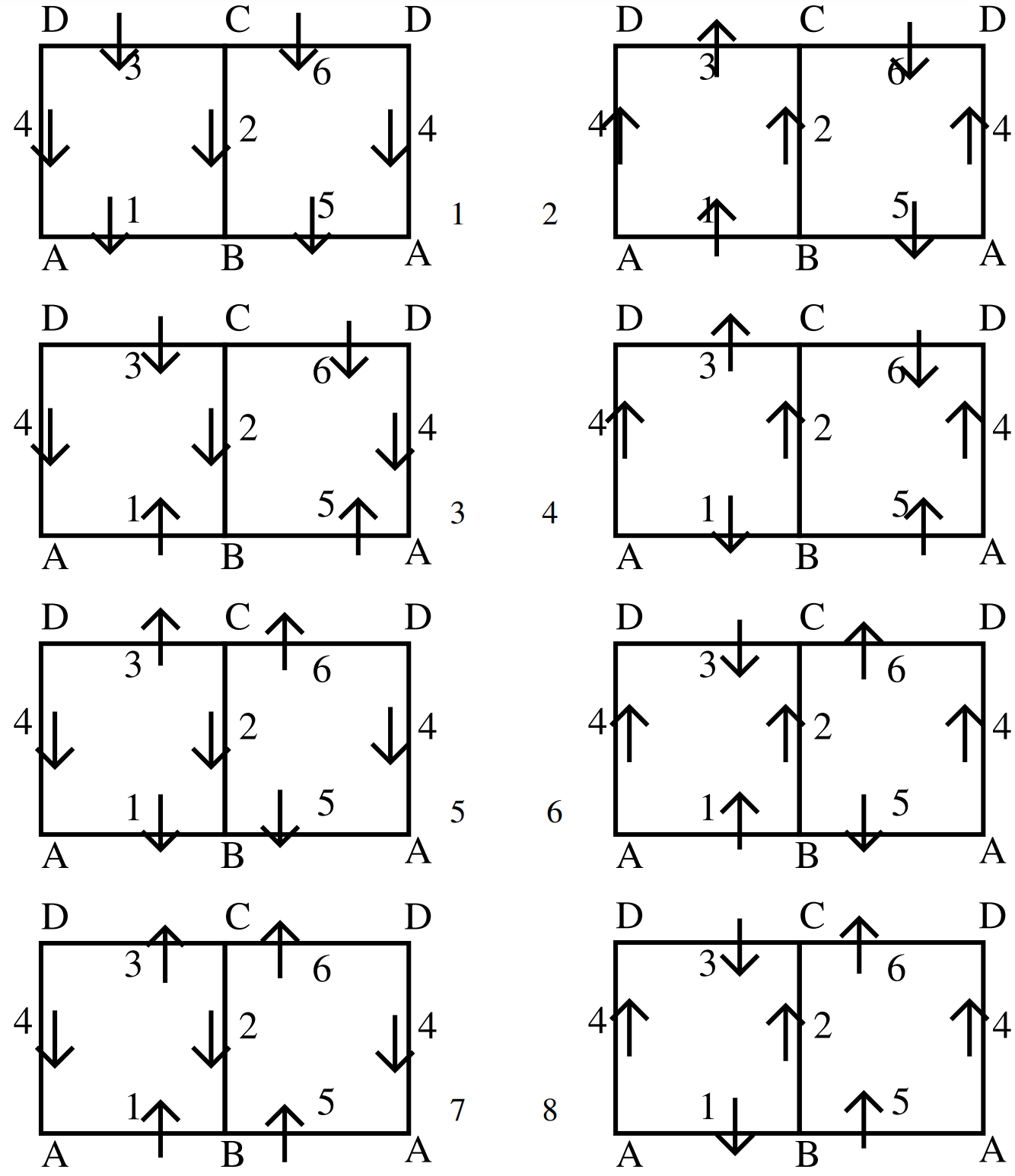
Figure 13: Basis states for the 2-plaquette $Z(2)$ lattice gauge theory. The up- and the down-spins are denoted in the x-basis.

On closer inspection it is clear that the basis states have another quantum number: these are the winding numbers of the $Z(2)$ strings along the lattice x- and y-directions respectively. The operators corresponding to these are simply the product of the $\sigma^{x}$ operators along a line which cuts the plaquettes horizontally and vertically respectively. For our case, the expressions for the operators are

$$W_{x} =\sigma^{x}_{4}\sigma^{x}_{2};\leavevmode\nobreak\ \leavevmode\nobreak\ \leavevmode\nobreak\ W_{y}=\sigma^{x}_{1}\sigma^{x}_{3};\leavevmode\nobreak\ \leavevmode\nobreak\ \leavevmode\nobreak\ W_{y}=\sigma^{x}_{5}\sigma^{x}_{6}.$$ (42)

The last two expressions for $W_{y}$ are actually the same as can be seen by using the Gauss law for the sites. The basis states $\ket{e_{1}},\ket{e_{2}},\ket{e_{7}},\ket{e_{8}}$ are in the sector $(1,1)$ while the rest $\ket{e_{3}},\ket{e_{4}},\ket{e_{5}},\ket{e_{6}}$ are in the sector $(1,-1)$. These sectors do not mix under a unitary (Hamiltonian) evolution.

The Hamiltonian has two terms: the first one will flip the spins 1,2,3, and 4 (since it is a $\sigma^{z}$), and the second one flips the spins 5,4,6, and 2. After this, one can compare the flipped state to the original one to find out the matrix elements. This gives the following Hamiltonian matrix:

$$H=\begin{bmatrix}0&-1&0&0&0&0&0&-1\\ -1&0&0&0&0&0&-1&0\\ 0&0&0&-1&0&-1&0&0\\ 0&0&-1&0&-1&0&0&0\\ 0&0&0&-1&0&-1&0&0\\ 0&0&-1&0&-1&0&0&0\\ 0&-1&0&0&0&0&0&-1\\ -1&0&0&0&0&0&-1&0\\ \end{bmatrix}$$ (43)

We implement a real-time quench: we start from a basis state in each (winding) sector and then compute the probability of finding the evolved wavefunction in the initial starting state. With a knowledge of the eigenvectors and eigenvalues of the matrix in Equation 43, which we denote as $\ket{\psi_{\rm n}}$, and with $\ket{\psi_{\rm i}}$ as the initial state

$$\begin{split}\ket{\psi(t)}&=\exp{-iHt}\ket{\psi_{\rm i}},\\ &=\exp{-iHt}\sum_{\rm n}\ket{\psi_{\rm n}}\braket{\psi_{\rm n}}{\psi_{\rm i}}\\ &=\sum_{\rm n}\exp{-iE_{\rm n}t}c_{\rm n}\ket{\psi_{\rm n}}\\ \braket{c_{\rm i}}{\psi(t)}&=\sum_{\rm n}|c_{\rm n}|^{2}\exp{-iE_{\rm n}t}\end{split}$$ (44)

where $c_{n}$ is the overlap of the initial starting state with that of the n-th eigenstate.

Appendix C Resource Scaling Calculations

In this section we count how many two-qubit gates will be needed for each qubit in order to simulate one Trotter step of the time-evolution for several different plaquette Hamiltonians, using the circuit identity (26). For simplicity in these calculations, we are considering only those qubits that correspond to physical links. The gate counting for ancillary qubit(s) will be different, but the gate number will change across the different Hamiltonians similarly to the way the physical-link-qubit gate counting will. Additionally (26) makes obvious that every two-qubit gate connected to an ancillary gate will also already be counted by counting two-qubit gates that are connected to physical-link-qubits.

Because the Hamiltonians we are discussing are always composed of plaquettes, and we are counting how many two-qubit gates are necessary per link, we first need to determine how many plaquettes touch a link as a function of the spatial dimension $d$.

We can do this by first considering a particular link $l$ and a point in it $x$, and noting that since there are $2d$ links that touch every point in a square lattice, there are thus $2d-1$ links other than $l$ that touch $x$. Each of these links–excluding the link that is co-linear with the chosen $l$–will then correspond to a unique plaquette that touches $l$. There are thus $2d-2$ plaquettes that touch each link in the lattice.

C.1 Quantum Link Models

For the $\mathbb{Z}_{2}$ quantum link model, we know from equations (2) and (3) that every plaquette has a single term corresponding to it that is a product of four Pauli-Z matrices. From Appendix A, we have seen that we can write the exponential of this product in the form of (26) where $N=4$. Thus one plaquette product term of four Pauli-Z matrices corresponds to two 2-qubit gates per physical-link-qubit. Thus there are $2(2d-2)$ two-qubit gates need for each physical-link-qubit, using the plaquette-per-link number computed above.

For the $U(1)$ quantum link model, we know from equation (16) that every plaquette has eight terms corresponding to it that are products of four Pauli matrices. This time they are not all Pauli-Z matrices, however rotation is an operation that necessitates only single-qubit gates, so it does not affect the two-qubit gate counting. Thus there will simply be eight times as many two-qubit gates per physical-link-qubit as were needed for the $\mathbb{Z}_{2}$ model, and so the counting is $8\cdot 2(2d-2)=16(2d-2)$ for the $U(1)$ quantum link model.

For the $SO(3)$ quantum link model, we can realize the symmetry by defining two rishons per link, and then each plaquette consists of eight rishons. The terms in the Hamiltonian corresponding to one plaquette are then

$$H_{\Box}=-\left(\vec{\sigma}_{R}^{1}\cdot\vec{\sigma}_{L}^{2}\right)\left(\vec{\sigma}_{R}^{2}\cdot\vec{\sigma}_{R}^{3}\right)\left(\vec{\sigma}_{L}^{3}\cdot\vec{\sigma}_{R}^{4}\right)\left(\vec{\sigma}_{L}^{4}\cdot\vec{\sigma}_{L}^{1}\right),$$ (45)

where $1,2,3,4$ correspond to links in a plaquette, and $R,L$ correspond to the two rishons in each link. The dot products are over the three Paul matrix directions $x,y,z$, so there are $3^{4}=81$ terms for every plaquette. The counting for each rishon-qubit (for a Trotter step) will thus be 81 times what is was for the $\mathbb{Z}_{2}$ case, and thus it will be $81\cdot 2(2d-2)=162(2d-2)$.

C.2 Kogut-Susskind Model

We next consider the counting for the potential energy (plaquette terms) of the Kogut-Susskind model [81], which can be written as for Abelian gauge groups:

$$V_{\mathrm{KS}}=-\alpha\sum_{\Box}\left(U_{1}U_{2}U^{\dagger}_{3}U^{\dagger}_{4}+{\mathrm{h.c.}}\right).$$ (46)

These $U$ operators are infinite dimensional in the full Hilbert space, but can be truncated to finite representations in order to obtain finite Hilbert space formulations amenable to quantum simulation.

For the $\mathbb{Z}_{2}$ theory, the smallest spin truncation possible yields $U_{i}=\sigma^{z}_{i}$, and the Hamiltonian is exactly the same as the QLM Hamiltonian. Thus as before we will need $2(2d-2)$ two-qubit gates for each physical-link-qubit.

For the $U(1)$ theory, the smallest spin representation possible is spin-1. We can then write the $U(1)$ theory in terms of $U_{i}(U^{\dagger}_{i})$, which is the raising (lowering) operator for the electric fluxes. In order to represent these three-state spins using qubits, we need two qubits per spin, which can be represented as [59]

$$U^{x}_{i} ={\sigma_{i}^{x}}^{(1)}\otimes\left({\mathbbm{1}_{i}}^{(2)}+{\sigma_{i}^{x}}^{(2)}+{\sigma_{i}^{z}}^{(2)}\right)/2$$ (47)

$$\qquad+{\sigma_{i}^{y}}^{(1)}\otimes{\sigma_{i}^{y}}^{(2)}/2,$$

$$U_{i}^{y} =-{\sigma_{i}^{y}}^{(1)}\otimes\left(\mathbbm{1}_{i}^{(2)}+{\sigma_{i}^{z}}^{(2)}-{\sigma_{i}^{x}}^{(2)}\right)/2$$

$$\qquad-{\sigma_{i}^{x}}^{(1)}\otimes{\sigma_{i}^{y}}^{(2)}/2.$$

From (16), we know that each plaquette will involve eight products of $U_{i}^{x/y}$ operators. Since each of these operators is itself a sum of four terms, there will be $2\cdot 8\cdot 4^{4}=2\cdot 2048$ two-qubit gates needed per qubit to produce one Trotter step of time evolution of the plaquette term. Combining this with the $(2d-2)$ number for the plaquettes that touch each link, we have that we need $2\cdot 2048(2d-2)$ two-qubit gates per physical-link-qubit.

C.3 Symanzik Improvement

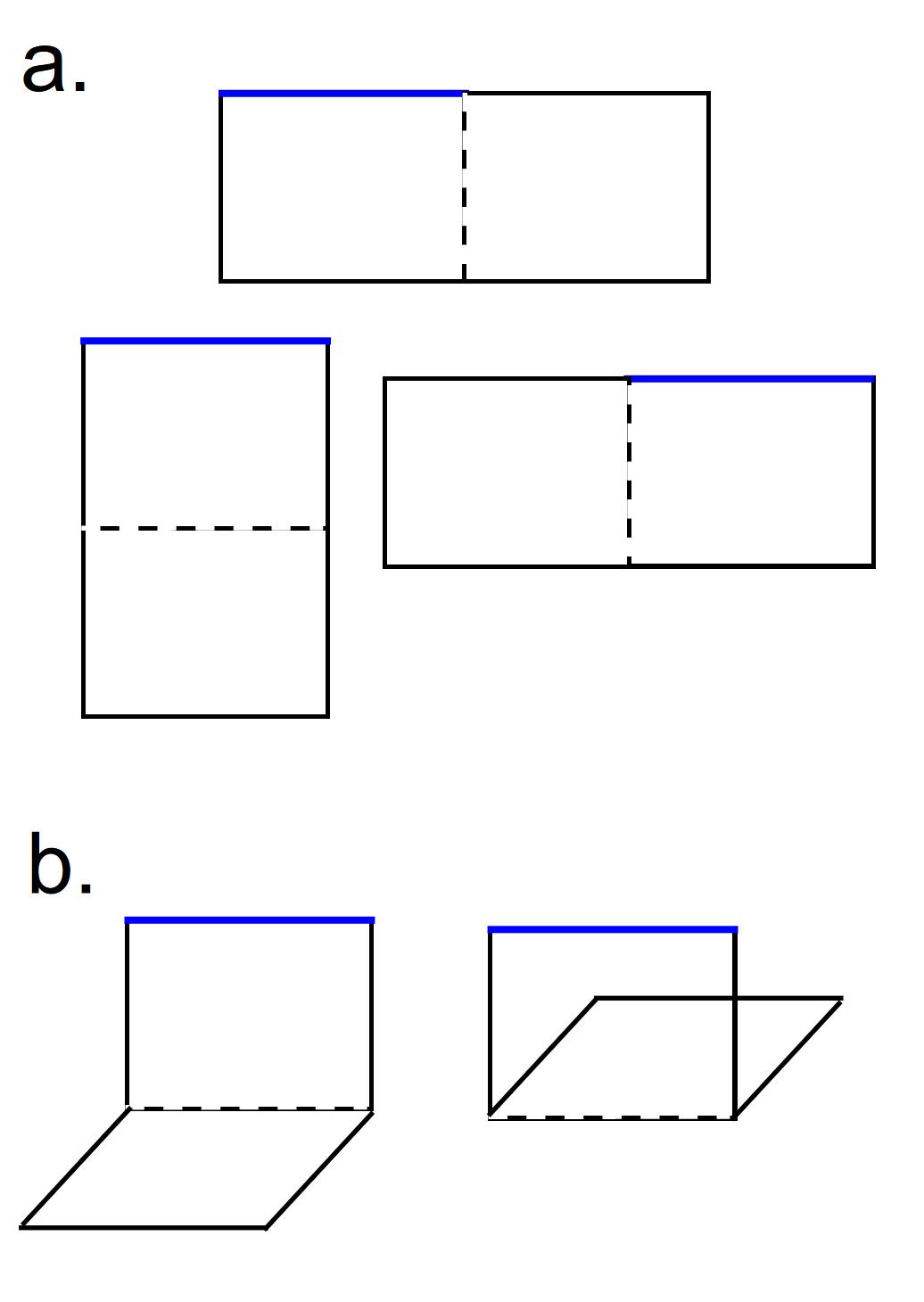
Figure 14: ($a$) Rectangular loops that touch the blue link that can be formed from one plaquette that touches the blue link. ($b$) Bent loops (for $d=2$) that touch the blue link that can be formed from one plaquette that touches the blue link.

Finally, we have that the Symanzik improvement [82] of the potential energy terms of the Kogut-Wilson Hamiltonian involves the addition of the following terms [58]:

$$V_{\mathrm{rect}} =\alpha_{1}\sum_{\mathrm{rect.\;loops}}\left(U_{1}U_{2}U_{3}U_{4}^{\dagger}U_{5}^{\dagger}U_{6}^{\dagger}+\mathrm{h.c.}\right)$$ (48)

$$V_{\mathrm{bent}} =\alpha_{2}\sum_{\mathrm{bent\;loops}}\left(U_{1}U_{2}U_{3}U_{4}^{\dagger}U_{5}^{\dagger}U_{6}^{\dagger}+\mathrm{h.c.}\right),$$

where the rectangular and bent loops are formed from two adjacent plaquettes (either within the same plane for the rectangular loops or in perpendicular planes for the bent loops). Diagrams illustrating these loops can be found in Fig. 14 [58].

Just as we did for the plaquettes, we first need to determine how many rectangular and bent loops touch each link. The rectangular loop can be viewed as a longer plaquette, and for every square plaquette that touches a link, there are three corresponding rectangular loops that touch that link (see Figure 14), because there are three sides of the first square plaquette that the second square plaquette can connect to. Thus there are $3(2d-2)$ rectangular loops that touch each linking, using the plaquette number from before. For the bent loops, there are $(2(d-1)-2)$ bent loops for every plaquette that touches a particular link (see Figure 14), and this can be seen from using the previous formula of $2d-2$ (for number of plaquettes that touch a link), to determine the number of plaquettes that touch a link of the first plaquette that are perpendicular to the first plaquette. Because they must be perpendicular to the first plaquette, we lose a dimension and the number is $2(d-1)-2=2d-4$. Thus the counting of bent plaquettes that touch a particular link is $(2d-4)(2d-2)$.

For the $\mathbb{Z}_{2}$ gauge theory, we recall that we used the representation where $U_{i}=\sigma_{i}^{z}$. From the numbers we just determined for the numbers of rectangular and bent plaquettes that touch a link, we can conclude that we need $2\cdot 3(2d-2)+2\cdot(2d-4)(2d-2)$ two-qubit gates per link-qubit per Trotter step.

For the $U(1)$ gauge theory, we know that $U_{i}$ can be written as $U^{+}_{i}$, and then writing in terms of $U^{x}_{i}$ and $U^{y}_{i}$ will lead to $2^{6}/2=32$ terms (similar to how 16 has $2^{4}/2=8$ terms). Because each $U^{x}_{i}$ and $U^{y}_{i}$ operator consists of four terms (47), there are $32\cdot 4^{6}=32\cdot 4096$ products of Pauli matrices per rectangular/bent loop. Thus there are $2\cdot 32\cdot 4096\cdot 3(2d-2)$ two-qubit gates per link needed for the rectangular loops, and $2\cdot 32\cdot 4096\;(2d-4)(2d-2)$ two-qubit gates per link needed for the bent loops, for one Trotter step of evolution.

Appendix D Fluctuations of IBM Q measurements

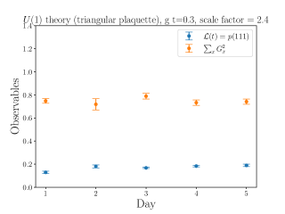
Figure 15: Data collected using IBM Q Quito over five consecutive days. The values for $\mathcal{L}(t)=p(111)$ are $0.13(1)$, $0.18(1)$, $0.168(5)$, $0.183(7)$, and $0.19(1)$. The values for $\sum_{x}G_{x}^{2}$ are $0.75(2)$, $0.72(5)$, $0.79(2)$, $0.73(2)$, and $0.74(2)$.

To illustrate how measurement values can change from one calibration to the next, we did the same measurements for the $U(1)$-theory on a triangular plaquette at a specific time and folding scale factor ($gt=0.3$, scale factor$=2.4$) over five consecutive days. The values we get for each day for two observables are plotted in Figure 15, and the observable values are written directly in the caption. We computed the average and error for each value of the observables by running the circuit for 8192 shots and five times within the same day. The measurements have also been corrected for readout error.

From the data we see that the measurements can vary substantially from each other from one calibration to the next. The largest difference in this example is between the measurements for $\mathcal{L}(t)=p(111)$ between Day 1 and Day 5, with the Day 5 measurement nearly $50\%$ larger than the Day 1 measurement. In taking our measurements and doing ZNE extrapolation for the figures in the main text, we made sure to take all scale factor measurements for a particular data point on the same day, so that the extrapolation would make sense for the noise of that day, but different time data for a time-evolution may come from different days, as for each individual model it took 1-2 weeks to run these jobs on the IBM Q hardware for the real time evolution of the observables over $gt\in[0,6]$ on a plaquette. While it would have been an improvement to then do an additional average over 5-10 calibration days, the time to run this would have been prohibitive with current queue wait time, and not indicative of what is straightforwardly achievable with this NISQ hardware.

References

- Wilczek [2016] F. Wilczek, Physica Scripta T168, 014003 (2016), URL https://doi.org/10.1088/0031-8949/t168/1/014003.
- Preskill [2018] J. Preskill, Quantum 2, 79 (2018), URL https://doi.org/10.22331/q-2018-08-06-79.
- Noh and Angelakis [2016] C. Noh and D. G. Angelakis, Reports on Progress in Physics 80, 016401 (2016), URL https://doi.org/10.1088/0034-4885/80/1/016401.
- Krantz et al. [2019] P. Krantz, M. Kjaergaard, F. Yan, T. P. Orlando, S. Gustavsson, and W. D. Oliver, Applied Physics Reviews 6, 021318 (2019), eprint https://doi.org/10.1063/1.5089550, URL https://doi.org/10.1063/1.5089550.
- Lanyon et al. [2011] B. P. Lanyon, C. Hempel, D. Nigg, M. Muller, R. Gerritsma, F. Zahringer, P. Schindler, J. T. Barreiro, M. Rambach, G. Kirchmair, et al., Science 334, 57–61 (2011), ISSN 1095-9203, URL http://dx.doi.org/10.1126/science.1208001.
- Bloch et al. [2012] I. Bloch, J. Dalibard, and S. Nascimbène, Nature Physics 8, 267 (2012), ISSN 1745-2481, number: 4 Publisher: Nature Publishing Group, URL https://www.nature.com/articles/nphys2259/boxes/briefing/signup/.
- Feynman [1982] R. P. Feynman, International Journal of Theoretical Physics 21, 467 (1982).
- Parra-Rodriguez et al. [2020] A. Parra-Rodriguez, P. Lougovski, L. Lamata, E. Solano, and M. Sanz, Physical Review A 101 (2020), ISSN 2469-9934, URL http://dx.doi.org/10.1103/PhysRevA.101.022305.
- Srednicki [1994] M. Srednicki, Phys. Rev. E 50, 888 (1994), URL https://link.aps.org/doi/10.1103/PhysRevE.50.888.
- Deutsch [1991] J. M. Deutsch, Phys. Rev. A 43, 2046 (1991), URL https://link.aps.org/doi/10.1103/PhysRevA.43.2046.
- Alet and Laflorencie [2018] F. Alet and N. Laflorencie, Comptes Rendus Physique 19, 498 (2018), ISSN 1631-0705, quantum simulation / Simulation quantique, URL http://www.sciencedirect.com/science/article/pii/S163107051830032X.
- Smith et al. [2016] J. Smith, A. Lee, P. Richerme, B. Neyenhuis, P. W. Hess, P. Hauke, M. Heyl, D. A. Huse, and C. Monroe, Nature Physics 12, 907 (2016), eprint 1508.07026.
- Serbyn et al. [2021] M. Serbyn, D. A. Abanin, and Z. Papić, Nature Physics 17, 675–685 (2021), ISSN 1745-2481, URL http://dx.doi.org/10.1038/s41567-021-01230-2.
- Bañuls et al. [2020] M. C. Bañuls et al., Eur. Phys. J. D 74, 165 (2020), eprint 1911.00003.
- Martinez et al. [2016] E. A. Martinez et al., Nature 534, 516 (2016), eprint 1605.04570.
- Bernien et al. [2017] H. Bernien, S. Schwartz, A. Keesling, H. Levine, A. Omran, H. Pichler, S. Choi, A. S. Zibrov, M. Endres, M. Greiner, et al., Nature 551, 579–584 (2017), ISSN 1476-4687, URL http://dx.doi.org/10.1038/nature24622.
- Schweizer et al. [2019] C. Schweizer, F. Grusdt, M. Berngruber, L. Barbiero, E. Demler, N. Goldman, I. Bloch, and M. Aidelsburger, Nature Physics 15, 1168–1173 (2019), ISSN 1745-2481, URL http://dx.doi.org/10.1038/s41567-019-0649-7.
- Mil et al. [2020] A. Mil, T. V. Zache, A. Hegde, A. Xia, R. P. Bhatt, M. K. Oberthaler, P. Hauke, J. Berges, and F. Jendrzejewski, Science 367, 1128 (2020), eprint 1909.07641.
- Yang et al. [2020] B. Yang, H. Sun, R. Ott, H.-Y. Wang, T. V. Zache, J. C. Halimeh, Z.-S. Yuan, P. Hauke, and J.-W. Pan, Nature 587, 392 (2020), eprint 2003.08945.
- Davoudi et al. [2020a] Z. Davoudi, M. Hafezi, C. Monroe, G. Pagano, A. Seif, and A. Shaw, Phys. Rev. Res. 2, 023015 (2020a), eprint 1908.03210.
- Lamm and Lawrence [2018] H. Lamm and S. Lawrence, Physical Review Letters 121 (2018), ISSN 1079-7114, URL http://dx.doi.org/10.1103/PhysRevLett.121.170501.
- Gustafson et al. [2019] E. Gustafson, Y. Meurice, and J. Unmuth-Yockey, Phys. Rev. D 99, 094503 (2019), eprint 1901.05944.
- Gustafson et al. [2021] E. Gustafson, P. Dreher, Z. Hang, and Y. Meurice (2021), eprint 1910.09478.
- Klco et al. [2018] N. Klco, E. F. Dumitrescu, A. J. McCaskey, T. D. Morris, R. C. Pooser, M. Sanz, E. Solano, P. Lougovski, and M. J. Savage, Physical Review A 98 (2018), ISSN 2469-9934, URL http://dx.doi.org/10.1103/PhysRevA.98.032331.
- Klco et al. [2020] N. Klco, M. J. Savage, and J. R. Stryker, Physical Review D 101 (2020), ISSN 2470-0029, URL http://dx.doi.org/10.1103/PhysRevD.101.074512.
- Zhang et al. [2018] J. Zhang, J. Unmuth-Yockey, J. Zeiher, A. Bazavov, S.-W. Tsai, and Y. Meurice, Physical Review Letters 121 (2018), ISSN 1079-7114, URL http://dx.doi.org/10.1103/PhysRevLett.121.223201.
- Lewis and Woloshyn [2019] R. Lewis and R. M. Woloshyn (2019), eprint 1905.09789.
- Atas et al. [2021] Y. Atas, J. Zhang, R. Lewis, A. Jahanpour, J. F. Haase, and C. A. Muschik (2021), eprint 2102.08920.
- Stryker [2019] J. R. Stryker, Phys. Rev. A 99, 042301 (2019), eprint 1812.01617.
- Raychowdhury and Stryker [2020a] I. Raychowdhury and J. R. Stryker, Phys. Rev. D 101, 114502 (2020a), eprint 1912.06133.
- Raychowdhury and Stryker [2020b] I. Raychowdhury and J. R. Stryker, Phys. Rev. Res. 2, 033039 (2020b), eprint 1812.07554.
- Davoudi et al. [2020b] Z. Davoudi, I. Raychowdhury, and A. Shaw (2020b), eprint 2009.11802.
- Klco and Savage [2019] N. Klco and M. J. Savage, Phys. Rev. A 99, 052335 (2019), eprint 1808.10378.
- Klco and Savage [2020] N. Klco and M. J. Savage, Phys. Rev. A 102, 052422 (2020), eprint 2002.02018.
- Ciavarella et al. [2021] A. Ciavarella, N. Klco, and M. J. Savage, Physical Review D 103 (2021), ISSN 2470-0029, URL http://dx.doi.org/10.1103/PhysRevD.103.094501.
- Bender and Zohar [2020] J. Bender and E. Zohar, Physical Review D 102 (2020), ISSN 2470-0029, URL http://dx.doi.org/10.1103/PhysRevD.102.114517.
- Aidelsburger et al. [2021] M. Aidelsburger, L. Barbiero, A. Bermudez, T. Chanda, A. Dauphin, D. González-Cuadra, P. R. Grzybowski, S. Hands, F. Jendrzejewski, J. Jünemann, et al. (2021), eprint 2106.03063.
- Zohar [2021] E. Zohar (2021), eprint 2106.04609.
- Kasper et al. [2020] V. Kasper, D. González-Cuadra, A. Hegde, A. Xia, A. Dauphin, F. Huber, E. Tiemann, M. Lewenstein, F. Jendrzejewski, and P. Hauke (2020), eprint 2010.15923.
- Funcke et al. [2021] L. Funcke, T. Hartung, K. Jansen, S. Kühn, and P. Stornati, Quantum 5, 422 (2021), ISSN 2521-327X, URL http://dx.doi.org/10.22331/q-2021-03-29-422.
- Shor [1995] P. W. Shor, Phys. Rev. A 52, R2493 (1995), URL https://link.aps.org/doi/10.1103/PhysRevA.52.R2493.
- Steane [1996] A. M. Steane, Phys. Rev. Lett. 77, 793 (1996), URL https://link.aps.org/doi/10.1103/PhysRevLett.77.793.
- Li and Benjamin [2017] Y. Li and S. C. Benjamin, Phys. Rev. X 7, 021050 (2017), URL https://link.aps.org/doi/10.1103/PhysRevX.7.021050.
- Kandala et al. [2019] A. Kandala, K. Temme, A. D. Córcoles, A. Mezzacapo, J. M. Chow, and J. M. Gambetta, Nature 567, 491–495 (2019), ISSN 1476-4687, URL http://dx.doi.org/10.1038/s41586-019-1040-7.
- He et al. [2020] A. He, B. Nachman, W. A. de Jong, and C. W. Bauer, Physical Review A 102 (2020), ISSN 2469-9934, URL http://dx.doi.org/10.1103/PhysRevA.102.012426.
- LaRose et al. [2020] R. LaRose, A. Mari, P. J. Karalekas, N. Shammah, and W. J. Zeng (2020), eprint 2009.04417.
- Giurgica-Tiron et al. [2020] T. Giurgica-Tiron, Y. Hindy, R. LaRose, A. Mari, and W. J. Zeng, 2020 IEEE International Conference on Quantum Computing and Engineering (QCE) (2020), URL http://dx.doi.org/10.1109/QCE49297.2020.00045.
- Lowe et al. [2020] A. Lowe, M. H. Gordon, P. Czarnik, A. Arrasmith, P. J. Coles, and L. Cincio, Unified approach to data-driven quantum error mitigation (2020), eprint 2011.01157.
- Sopena et al. [2021] A. Sopena, M. H. Gordon, G. Sierra, and E. López, Simulating quench dynamics on a digital quantum computer with data-driven error mitigation (2021), eprint 2103.12680.
- McArdle et al. [2019] S. McArdle, X. Yuan, and S. Benjamin, Phys. Rev. Lett. 122, 180501 (2019), URL https://link.aps.org/doi/10.1103/PhysRevLett.122.180501.
- Funcke et al. [2020] L. Funcke, T. Hartung, K. Jansen, S. Kühn, P. Stornati, and X. Wang, Measurement error mitigation in quantum computers through classical bit-flip correction (2020), eprint 2007.03663.
- Nachman et al. [2020] B. Nachman, M. Urbanek, W. A. de Jong, and C. W. Bauer, npj Quantum Information 6, 84 (2020), ISSN 2056-6387, URL https://doi.org/10.1038/s41534-020-00309-7.
- Jattana et al. [2020] M. S. Jattana, F. Jin, H. De Raedt, and K. Michielsen, Quantum Information Processing 19, 414 (2020), ISSN 1573-1332, URL https://doi.org/10.1007/s11128-020-02913-0.
- Klco and Savage [2021] N. Klco and M. J. Savage (2021), eprint 2109.01953.
- Horn [1981] D. Horn, Phys. Lett. 100B, 149 (1981).
- Orland and Rohrlich [1990] P. Orland and D. Rohrlich, Nucl. Phys. B338, 647 (1990).
- Chandrasekharan and Wiese [1997] S. Chandrasekharan and U. J. Wiese, Nucl. Phys. B492, 455 (1997), eprint hep-lat/9609042.
- Carena et al. [2022] M. Carena, H. Lamm, Y.-Y. Li, and W. Liu (2022), eprint 2203.02823.
- Gustafson [2021] E. J. Gustafson, Phys. Rev. D 103, 114505 (2021), URL https://link.aps.org/doi/10.1103/PhysRevD.103.114505.
- Rico et al. [2018] E. Rico, M. Dalmonte, P. Zoller, D. Banerjee, M. Bögli, P. Stebler, and U.-J. Wiese, Annals of Physics 393, 466–483 (2018), ISSN 0003-4916, URL http://dx.doi.org/10.1016/j.aop.2018.03.020.
- Müller et al. [2011] M. Müller, K. Hammerer, Y. L. Zhou, C. F. Roos, and P. Zoller, New Journal of Physics 13, 085007 (2011), eprint 1104.2507.
- Mezzacapo et al. [2015] A. Mezzacapo, E. Rico, C. Sabín, I. L. Egusquiza, L. Lamata, and E. Solano, Phys. Rev. Lett. 115, 240502 (2015), eprint 1505.04720.
- Kitaev [2003] A. Kitaev, Annals of Physics 303, 2–30 (2003), ISSN 0003-4916, URL http://dx.doi.org/10.1016/S0003-4916(02)00018-0.
- Shannon et al. [2004] N. Shannon, G. Misguich, and K. Penc, Phys. Rev. B 69, 220403 (2004), URL https://link.aps.org/doi/10.1103/PhysRevB.69.220403.
- Hermele et al. [2004] M. Hermele, M. P. A. Fisher, and L. Balents, Physical Review B 69 (2004), ISSN 1550-235X, URL http://dx.doi.org/10.1103/PhysRevB.69.064404.
- Brower et al. [2020] R. C. Brower, D. Berenstein, and H. Kawai, Lattice gauge theory for a quantum computer (2020), eprint 2002.10028.
- Banerjee et al. [2021] D. Banerjee, S. Caspar, F. J. Jiang, J. H. Peng, and U. J. Wiese (2021), eprint 2107.01283.
- Heyl [2019] M. Heyl, EPL (Europhysics Letters) 125, 26001 (2019), URL https://doi.org/10.1209/0295-5075/125/26001.
- Banerjee et al. [2013] D. Banerjee, F.-J. Jiang, P. Widmer, and U.-J. Wiese, Journal of Statistical Mechanics: Theory and Experiment 2013, P12010 (2013), ISSN 1742-5468, URL http://dx.doi.org/10.1088/1742-5468/2013/12/P12010.
- Banerjee and Sen [2021] D. Banerjee and A. Sen, Physical Review Letters 126 (2021), ISSN 1079-7114, URL http://dx.doi.org/10.1103/PhysRevLett.126.220601.
- Marcos et al. [2014] D. Marcos, P. Widmer, E. Rico, M. Hafezi, P. Rabl, U. J. Wiese, and P. Zoller, Annals of Physics 351, 634 (2014), eprint 1407.6066.
- Glaetzle et al. [2015] A. W. Glaetzle, M. Dalmonte, R. Nath, C. Gross, I. Bloch, and P. Zoller, Physical Review Letters 114 (2015), ISSN 1079-7114, URL http://dx.doi.org/10.1103/PhysRevLett.114.173002.
- Celi et al. [2020] A. Celi, B. Vermersch, O. Viyuela, H. Pichler, M. D. Lukin, and P. Zoller, Physical Review X 10 (2020), ISSN 2160-3308, URL http://dx.doi.org/10.1103/PhysRevX.10.021057.
- Linke et al. [2017] N. M. Linke, D. Maslov, M. Roetteler, S. Debnath, C. Figgatt, K. A. Landsman, K. Wright, and C. Monroe, Proceedings of the National Academy of Sciences 114, 3305 (2017), ISSN 0027-8424, eprint https://www.pnas.org/content/114/13/3305.full.pdf, URL https://www.pnas.org/content/114/13/3305.
- Cross et al. [2019] A. W. Cross, L. S. Bishop, S. Sheldon, P. D. Nation, and J. M. Gambetta, Phys. Rev. A 100, 032328 (2019), URL https://link.aps.org/doi/10.1103/PhysRevA.100.032328.
- Chen and et. al. [2021] Z. Chen and et. al., Nature 595, 383 (2021), ISSN 1476-4687, URL https://doi.org/10.1038/s41586-021-03588-y.
- Geller [2020] M. R. Geller, Quantum Science and Technology 5, 03LT01 (2020), eprint 2002.01471.
- Maciejewski et al. [2020] F. B. Maciejewski, Z. Zimborás, and M. Oszmaniec, Quantum 4, 257 (2020), ISSN 2521-327X, URL https://doi.org/10.22331/q-2020-04-24-257.
- et. al. [2021] M. S. A. et. al., Qiskit: An Open-source Framework for Quantum Computing (2021).
- Brower et al. [1999] R. Brower, S. Chandrasekharan, and U.-J. Wiese, Physical Review D 60 (1999), ISSN 1089-4918, URL http://dx.doi.org/10.1103/PhysRevD.60.094502.
- Kogut and Susskind [1975] J. Kogut and L. Susskind, Phys. Rev. D 11, 395 (1975), URL https://link.aps.org/doi/10.1103/PhysRevD.11.395.
- Symanzik [1983] K. Symanzik, Nuclear Physics B 226, 187 (1983), ISSN 0550-3213, URL https://www.sciencedirect.com/science/article/pii/0550321383904686.